Conservative and Risk-Aware Offline Multi-Agent Reinforcement Learning for Digital Twins

Abstract

Digital twin (DT) platforms are increasingly regarded as a promising technology for controlling, optimizing, and monitoring complex engineering systems such as next-generation wireless networks. An important challenge in adopting DT solutions is their reliance on data collected offline, lacking direct access to the physical environment. This limitation is particularly severe in multi-agent systems, for which conventional multi-agent reinforcement (MARL) requires online interactions with the environment. A direct application of online MARL schemes to an offline setting would generally fail due to the epistemic uncertainty entailed by the limited availability of data. In this work, we propose an offline MARL scheme for DT-based wireless networks that integrates distributional RL and conservative Q-learning to address the environment’s inherent aleatoric uncertainty and the epistemic uncertainty arising from limited data. To further exploit the offline data, we adapt the proposed scheme to the centralized training decentralized execution framework, allowing joint training of the agents’ policies. The proposed MARL scheme, referred to as multi-agent conservative quantile regression (MA-CQR) addresses general risk-sensitive design criteria and is applied to the trajectory planning problem in drone networks, showcasing its advantages.

I Introduction

I-A Context and Motivation

Recent advances in machine learning (ML), high-performance computing, cloudification, and simulation intelligence [1] have supported the development of a novel data-driven paradigm for the design, monitoring, and control of physical systems: digital twin (DT) platforms  [2, 3]. A DT system consists of a digital mirror of the physical twin (PT) counterpart built and maintained using data from the PT. Originating in manufacturing, DTs have emerged as a promising solution for fields such as healthcare and next-generation wireless networks, allowing algorithms and ML models to be optimized and tested virtually before deployment on the PT [4, 5]. In the context of wireless networks, DTs are particularly well suited as a component in open radio access network architectures (RANs) [6, 7].

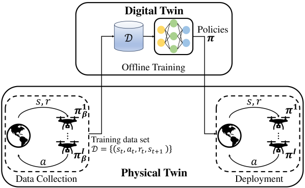
Figure 1: A digital twin of a physical system may only have access to data collected offline following some fixed and unknown policies $\pi_{\beta}=\{\pi_{\beta}^{i}\}^{I}_{i=1}$ at the physical twin consisting of $I$ agents. Based on this dataset, the digital twin wishes to optimize policies $\pi=\{\pi^{i}\}^{I}_{i=1}$ for the physical system while ensuring robustness to the uncertainty arising from the stochastic environment, from the limited data, and from the lack of interactions with the environment.

The DT generally updates its internal representation of the PT and the ML models being trained on behalf of the PT based on data received from the PT. The process of synchronizing the DT is limited by the communication bottleneck between DT and PT [7, 8]. As a result, an important challenge in adopting DT solutions is their reliance on data collected offline, lacking direct access to the physical system. This limitation is particularly severe in multi-agent systems, for which conventional multi-agent reinforcement (MARL) requires online interactions with the environment [9].

A direct application of online MARL schemes to an offline setting would generally fail due to the epistemic uncertainty entailed by the limited availability of data. In particular, even in the case of a single agent, offline reinforcement learning (RL) may over-estimate the quality of given actions that happened to perform well during data collection due to the inherent stochasticity and outliers of the environment [10]. This problem can be addressed in online RL via exploration, trying actions, and modifying return estimates based on environmental feedback. However, exploration is not feasible in offline RL, as policy design is based solely on the offline dataset. Furthermore, in multi-agent systems, this problem is exacerbated by the inherent uncertainty caused by the non-stationary behavior of other agents during training [11, Chapter 11].

In this paper, we propose a novel offline MARL strategy that addresses the overall uncertainty at the DT about the impact of actions on the PT. The introduced approaches are termed multi-agent conservative independent quantile regression (MA-CIQR) via independent learning and multi-agent conservative centralized quantile regression (MA-CCQR) via centralized training and decentralized execution. These aproaches integrate distributional RL [11] and offline RL [12] to support a risk-sensitive multi-agent design that mitigates impairments arising from access to limited data from the PT. We showcase the performance of MA-CIQR and MA-CCQR by focusing on the problem of designing trajectories of unmanned aerial vehicles (UAVs) used to collect data from sensors in an Internet-of-Things (IoT) scenario [13, 14, 15] (see Fig. 1).

I-B Offline RL and Distributional RL

Offline RL has gained increasing interest in recent years due to its wide applicability to domains where online interaction with the environment is impossible or presents high costs and risks. Offline RL relies on a static offline transition dataset collected from the PT using some behavioral policy. The behavioral policy is generally suboptimal and may be unknown to the designer [10]. The reliance on a suboptimal policy for data collection distinguishes offline RL from imitation learning, in which the goal is reproducing the behavior of an expert policy [16]. The discrepancy between the behavior and optimized policies creates a distributional shift between training data and design objective. This shift could be resolved by collecting more data, but this is not possible in an offline setting. Therefore, the distributional shift contributes to the epistemic uncertainty of the agent.

Several approaches have been proposed to address this problem in offline RL. One class of methods constrains the difference between the learned and behavior policies [17]. Another popular approach is to learn conservative estimates of the action-value function or Q-function. Specifically, conservative Q-learning (CQL), proposed in [12], penalizes the values of the Q-function for out-of-distribution (OOD) actions. OOD actions are those whose impact is not sufficiently covered by the data set.

Apart from offline RL via CQL, the proposed scheme builds on distributional RL (DRL), which is motivated by the inherent aleatoric uncertainty caused by the stochasticity of the environment [18, 19, 20]. Rather than targeting the average return as in conventional RL, DRL maintains an estimate of the distribution of the return. This supports the design of risk-sensitive policies that disregard gains attained via risky behavior, favoring policies that ensure satisfactory worst-case performance levels instead.

A popular risk measure for use in DRL is the conditional value at risk (CVaR) [21, 22, 20, 23], which evaluates the average performance by focusing only on the lower tail of the return distribution. Furthermore, a state-of-the-art DRL strategy is quantile-regression deep Q-network (QR-DQN), which approximates the return distribution by estimating $N$ uniformly spaced quantiles [19].

I-C Related Work

Offline MARL: Offline MARL solutions have been proposed in several previous works by adapting the idea of conservative offline learning to the context of multi-agent systems [24, 25, 26, 27, 28]. Specifically, conservative estimates of the value function in a decentralized fashion are obtained in [24] via value deviation and transition normalization. Several other works proposed centralized learning approaches. The authors in [25] leveraged first-order policy gradients to calculate conservative estimates of the agents’ value functions. The work [26] presented a counterfactual conservative approach for offline MARL, while [27] introduced a framework that converts global-level value regularization into equivalent implicit local value regularization. The authors in [28] addressed the overestimation problem using implicit constraints.

Overall, all of these works focused on risk-neutral objectives, hence not making any provisions to address risk-sensitive criteria such as CVaR. In this regard, the paper [23] combined distributional RL and conservative Q-learning to develop a risk-sensitive algorithm, but only for single-agent settings.

Regarding applications of offline RL to wireless systems, the recent work [29] investigated a radio resource management problem by comparing the performance of several single-agent offline RL algorithms.

Applications of MARL to wireless systems: Due to the multi-objective and multi-agent nature of many control and optimization problems in wireless networks, MARL has been adopted as a promising solution in recent years. For instance, related to our contribution, the work in [30] proposed an online MARL algorithm to jointly minimize the age-of-information (AoI) and the transmission power in IoT networks with traffic arrival prediction, whereas the authors in [31] leveraged MARL for AoI minimization in UAV-to-device communications. Moreover, MARL was used in [32] for resource allocation in UAV networks. The work [33] developed a MARL-based solution for optimizing power allocation dynamically in wireless systems. The authors in [34] used MARL for distributed resource management and interference mitigation in wireless networks.

Applications of distributional RL to wireless systems: Distributional RL has been recently leveraged in [35] to carry out the optimization for a downlink multi-user communication system with a base station assisted by a reconfigurable intelligent reflector (IR). Meanwhile, reference [36] focused on the case of mmWave communications with IRs on a UAV. Distributional RL has also been used in [37] for resource management in network slicing.

All in all, to the best of our knowledge, our work in this paper is the first to integrate conservative offline RL and distributional MARL, and it is also the first to investigate the application of offline MARL to wireless systems.

I-D Main Contributions

This work introduces MA-CQR, a novel offline MARL scheme that supports optimizing risk-sensitive design criteria such as CVaR. MA-CQR is evaluated on the relevant problem of UAV trajectory design for IoT networks. The contributions of this paper are summarized as follows.

• We propose MA-CQR, a novel conservative and distributional offline MARL solution. MA-CQR leverages quantile regression (QR) to support the optimization of risk-sensitive design criteria and CQL to ensure robustness to OOD actions. As a result, MA-CQR addresses both the epistemic uncertainty arising from the presence of limited data and the aleatoric uncertainty caused by the randomness of the environment.

• We present two versions of MA-CQR with different levels of coordination among the agents. In the first version, referred to as MA-CIQR, the agents’ policies are optimized independently. In the second version, referred to as MA-CCQR, we leverage value decomposition techniques that allow centralized training and decentralized execution [38].

• To showcase the proposed schemes, we consider atrajectory optimization problem in UAV networks [30]. As illustrated in Fig. 1, the system comprises multiple UAVs collecting information from IoT devices. The multi-objective design tackles the minimization of the AoI for data collected from the devices and the overall transmit power consumption. We specifically exploit MA-CQR to design risk-sensitive policies that avoid excessively risky trajectories in the pursuit of larger average returns.

• Numerical results demonstrate that MA-CIQR and MA-CCQR versions yield faster convergence and higher returns than the baseline algorithms. Furthermore, both schemes can avoid risky trajectories and provide the best worst-case performance. Experiments also depict that centralized training provides faster convergence and requires less offline data.

The rest of the paper is organized as follows. Section II describes the MARL setting and the design objective. Section III introduces distributional RL and conservative Q-Learning. In section IV, we present the proposed MA-CQR algorithm. In Section VI, we provide numerical experiments on trajectory optimization in UAV networks. Section VII concludes the paper.

TABLE I: Abbreviations

AoI	Age-of-information
CDF	Cumulative distribution function
CQL	Conservative Q-learning
CTDE	Centralized training and decentralized execution
CVaR	Conditional value at risk
DQN	Deep Q-networks
DRL	Distributional reinforcement learning
DT	Digital twin
MA-CCQL	Multi-agent conservative centralized Q-learning
MA-CCQR	Multi-agent conservative centralized quantile regression
MA-CIQL	Multi-agent conservative independent Q-learning
MA-CIQR	Multi-agent conservative independent quantile regression
MA-CQR	Multi-agent conservative quantile regression
MARL	Multi-agent reinforcement learning
OOD	Out-of-distribution
PT	Physical twin
QR-DQN	Quantile-regression DQN
UAV	Unmanned aerial vehicles

TABLE II: Notations

$I$	Number of agents
$s_{t}$	Overall state of the PT system at time step $t$
$a_{t}$	Joint action of all agents at time step $t$
$a_{t}^{i}$	Action of agent $i$ at time step $t$
$r_{t}$	Immediate reward at time step $t$
$\gamma$	Discount factor
$Q(s,a)$	Q-function
$Z(s,a)$	Return starting from $(s,a)$
$P(s_{t+1}|s_{t},a_{t})$	Transition probability
$\pi^{i}(a^{i}_{t}\mid s_{t})$	Policy of agent $i$
$P_{Z(s,a)}$	Distribution of the return
$R(r_{t}\mid s_{t},a_{t})$	Stationary reward distribution
$\xi$	Risk tolerance level
$J_{\xi}^{\text{CVaR}}$	CVaR risk measure
$F_{Z^{\pi}}^{-1}\big{(}\xi\big{)}$	Inverse CDF of the return
$\mathcal{D}$	Offline dataset collected at the PT
$\theta_{j}^{i}(s,a)$	Quantile estimate of the distribution $P_{Z^{i}(s,a)}(\theta^{i})$
$\zeta_{\tau}(u)$	Quantile regression Huber loss
$\Delta^{i(k)}_{jj^{\prime}}$	TD errors evaluated with the quantile estimates
	of agent $i$
$\alpha$	CQL hyperparameter
$M$	Number of devices in the system
$A_{t}^{m}$	AoI of device $m$ at time step $t$
$g_{t}^{i,m}$	Channel gain between agent $i$ and device $m$
	at time step $t$
$P_{t}^{i,m}$	Transmission power for device $m$ to communicate with
	agent $i$ at time step $t$
$p_{\mathrm{risk}}$	Risk probability
$\mathrm{P_{\mathrm{risk}}}$	Risk penalty

II Problem Definition

We consider the setting illustrated in Fig. 1, where $I$ agents act in a physical environment that evolves in discrete time as a function of the agents’ actions and random dynamics. The design of the agents’ policies $\pi=\{\pi^{i}\}_{i=1}^{I}$ is carried out at a central unit – the digital twin (DT) in Fig. 1 – that has only access to a fixed dataset $\mathcal{D}$, while not being able to interact with the physical system. The dataset $\mathcal{D}$ is collected offline by allowing the agents to act in the environment according to arbitrary, fixed, and generally unknown policies $\pi_{\beta}=\{\pi_{\beta}^{i}\}_{i=1}^{I}$. In this section, we describe the multi-agent setting and formulate the offline learning problem. Tables I and II summarize the list of abbreviations and notations.

II-A Multi-Agent Setting

Consider an environment characterized by a time-variant state $s_{t}$, where $t=1,2,...$ is the discrete time index. At time step $t$, each agent $i$ takes action $a^{i}_{t}\in\mathcal{A}^{i}$ within some discrete action space $\mathcal{A}^{i}$. We denote by $a_{t}=\big{[}a_{t}^{1},\cdots,a_{t}^{I}\big{]}$ the vector of actions of all agents at timestep $t$. The state $s_{t}$ evolves according to a transition probability $P(s_{t+1}|s_{t},a_{t})$ as a function of the current state $s_{t}$ and of the action vector $a_{t}$. The transition probability $P(s_{t+1}|s_{t},a_{t})$ is stationary, i.e., it does not vary with time index $t$.

We focus on a fully observable multi-agent reinforcement learning setting, in which each agent $i$ has access to the full system state $s_{t}$ and produces action $a_{t}^{i}$ by following a policy $\pi^{i}(a^{i}_{t}\mid s_{t})$.

II-B Design Goal

As illustrated in Fig. 1, the DT aims at finding the optimal policies $\pi_{*}(a|s)=\{\pi_{*}^{i}(a|s)\}_{i=1}^{I}$ that maximize a risk measure $\rho(\cdot)$ of the return $Z^{\pi}=\sum_{t=0}^{\infty}\gamma^{t}r_{t}$, which we write as

$$J_{\rho}(\pi)=\rho\left[Z^{\pi}\right],$$ (1)

where $0<\gamma<1$ is a given discount factor. The distribution of the return $Z^{\pi}$ depends on the policies $\pi$ through the distribution of the trajectory $\mathcal{T}=(s_{0},a_{0},r_{0},s_{1},a_{1},r_{1},...)$, which is given by

$$P({\mathcal{T}})=P(s_{0})\prod_{t=0}^{\infty}\pi(a_{t}\mid s_{t})R(r_{t}\mid s_{t},a_{t})P(s_{t+1}\mid s_{t},a_{t}),$$ (2)

with $\pi(a_{t}\mid s_{t})=\prod_{i=1}^{I}\pi^{i}(a_{t}^{i}\mid s_{t})$ being the joint conditional distribution of the agents’ actions; $P(s_{0})$ being a fixed initial distribution; and $R(r_{t}\mid s_{t},a_{t})$ being the stationary reward distribution.

The standard choice for the risk measure in (1) is the expectation $\rho[\cdot]=\mathbb{E}[\cdot]$, yielding the standard criterion

$$J^{\text{avg}}(\pi)=\mathbb{E}\big{[}Z^{\pi}\big{]}.$$ (3)

The average criterion in (3) is considered to be risk neutral, as it does not directly penalize worst-case situations, catering only to the average performance.

In stochastic environments where the level of aleatoric uncertainty caused by the transition probability and/or the reward distribution is high, maximizing the expected return may not be desirable since the return $Z^{\pi}$ has high variance. In such scenarios, designing risk-sensitive policies may be preferable to enhance the worst-case outcomes while reducing the average performance (3).

A common risk-sensitive measure is the conditional value-at-risk (CVaR) [21], which is defined as the conditional mean

$$J_{\xi}^{\text{CVaR}}(\pi)=\mathbb{E}\big{[}Z^{\pi}\mid Z^{\pi}\leq F_{Z^{\pi}}^{-1}\big{(}\xi\big{)}\big{]},$$ (4)

where $F_{Z^{\pi}}^{-1}\big{(}\xi\big{)}$ is the inverse cumulative distribution function (CDF) of the return ${Z^{\pi}}$ for some $\xi\in[0,1]$, i.e., the $\xi$-th quantile of the distribution of the return. The CVaR, illustrated in Fig. 2, focuses on the lower tail of the return distribution by neglecting values of the return that are larger than the $\xi$-th quantile $F_{Z^{\pi}}^{-1}\big{(}\xi\big{)}$. Accordingly, the probability $\xi$ represents the risk tolerance level, with $\xi=1$ recovering the risk-neutral objective (3). The CVaR can also be written as the integral of the quantile function $F_{Z^{\pi}}^{-1}(\xi)$ as

$$J_{\xi}^{\text{CVaR}}(\pi)=\frac{1}{\xi}\int_{0}^{\xi}F_{Z^{\pi}}^{-1}(u)\text{d}u.$$ (5)

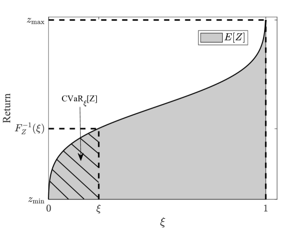
Figure 2: Illustration of the conditional value-at-risk (CVaR). The quantile function $F_{Z}^{-1}(\xi)$ is plotted as a function of the risk tolerance level $\xi$. The shaded area representing the lower tail of the distribution depicts the $\xi$-level CVaR.

II-C Offline Multi-Agent Reinforcement Learning

Conventional MARL [39] assumes that agents optimize their policies $\pi=\{\pi^{i}(a\mid s)\}_{i=1}^{I}$ via an online interaction with the environment, allowing for the exploration of new actions $a_{t}$ as a function the state $s_{t}$. In this paper, as illustrated in Fig. 1, we assume that the design of policies is carried out at the DT on the basis solely of the availability of an offline dataset $\mathcal{D}=\{(s,a,r,s^{\prime})\}$ of transitions $(s,a,r,s^{\prime})$. Each transition follows the stationary marginal distribution from (2), with policy $\pi(a|s)$ given by the fixed and unknown behavior policy $\pi_{\beta}(a|s)=\prod_{i=1}^{I}\pi_{\beta}^{i}(a^{i}|s)$.

III Background

In this section, we present a brief review of distributional RL, as well as of offline RL via CQL for a single agent model [12]. This material will be useful to introduce the proposed multi-agent offline DRL solution in the next section.

III-A Distributional Reinforcement Learning

Distributional RL aims at optimizing the agent’s policy, $\pi$, while accounting for the inherent aleatoric uncertainty associated with the stochastic environment. To this end, it tracks the return’s distribution, allowing the minimization of an arbitrary risk measure, such as the CVaR.

To elaborate, let us denote the random variable representing the return starting from a given state-action pair $(s,a)$ as $Z^{\pi}(s,a)$. Taking the expectation of the return $Z^{\pi}(s,a)$ over distribution (2) yields the state-action value function, also known as Q-function, as

$$Q^{\pi}(s,a)=\mathbb{E}\left[Z^{\pi}(s,a)\right].$$ (6)

Classical Q-learning algorithms learn the optimal policy $\pi^{*}$ by finding the optimal Q-function $Q(s,a)$ as the unique fixed point of the Bellman optimality operator [40]

$$Q(s,a)=\mathbb{E}\left[r+\gamma\>\max_{a^{\prime}\in\mathcal{A}}Q(s^{\prime},a^{\prime})\right],$$ (7)

with average evaluated with respect to the random variables $(r,s^{\prime})\sim R(r|s,a)P(s^{\prime}|s,a)$. The optimal policy $\pi^{*}$ for the average criterion (3) is directly obtained from the optimal Q-function as

$$\pi^{*}(a|s)=\mathbbm{1}\left\{a={\operatorname{arg}\,\max_{a\in\mathcal{A}}}\,\ Q(s,a)\right\},$$ (8)

with $\mathbbm{1}\{\cdot\}$ being the indicator function.

Similarly, for any risk measure $\rho[\cdot]$, one can define the distributional Bellman optimality operator for the random return $Z(s,a)$ as [18, 19]

$$Z(s,a)\overset{D}{=}r+\gamma\>Z\left(s^{\prime},{\operatorname{arg}\,\max_{a^{\prime}\in\mathcal{A}}}\,\ \rho[Z(s^{\prime},a^{\prime})]\right),$$ (9)

where equality holds regarding the distribution of the random variables on the left- and right-hand sides, and the random variables $(r,s^{\prime})$ are distributed as in (7). The optimal policy for the general criterion (1) can be expressed directly as a function of the optimal $Z(s,a)$ in (9) as [18, 19]

$$\pi(a|s)=\mathbbm{1}\left\{a={\operatorname{arg}\,\max_{a\in\mathcal{A}}}\,\rho[Z(s,a)]\right\}.$$

Quantile regression DQN (QR-DQN) [19] estimates the distribution $P_{Z(s,a)}$ of the optimal return $Z(s,a)$ by approximating it via a uniform mixture of Dirac functions centered at $N$ values $\{\theta_{j}(s,a)\}_{j=1}^{N}$, i.e.,

$$\hat{P}_{Z(s,a)}(\theta)=\frac{1}{N}\sum_{j=1}^{N}\delta_{\theta_{j}(s,a)}.$$ (10)

Each value $\theta_{j}(s,a)$ in (10) is an estimate of the quantile $F^{-1}_{{Z(s,a)}}(\hat{\tau}_{j})$ of distribution ${P}_{Z(s,a)}$ corresponding to the quantile target $\hat{\tau}_{j}=(\tau_{j-1}-\tau_{j})/2$, with $\tau_{j}=j/N$ for $1\leq j\leq N$. Note that $\{\theta_{j}(s,a)\}_{j=1}^{N}$ are estimated via quantile regression, which is achieved by modeling the function mapping $(s,a)$ to the $N$ values $\{\theta_{j}(s,a)\}_{j=1}^{N}$ as a neural network [19], which takes a state as input, and outputs the estimated $\theta_{j}(s,a)$ for all actions $a\in\mathcal{A}$ .

The neural network is trained by minimizing the loss

$$\frac{1}{N^{2}}\sum_{j=1}^{N}\sum_{j^{\prime}=1}^{N}\zeta_{\hat{\tau}_{j}}\left(\Delta_{jj^{\prime}}\right),$$

where $\Delta_{jj^{\prime}}$ are the temporal difference (TD) errors corresponding to the quantile estimates, i.e.,

$$\Delta_{jj^{\prime}}=r+\gamma{\theta}_{j^{\prime}}(s^{\prime},a^{\prime})-\theta_{j}^{i}(s,a^{i}),$$ (11)

with $a^{\prime}={\operatorname{arg}\,\max_{a\in\mathcal{A}}}\,\frac{1}{N}\sum_{j^{\prime}=1}^{N}{\theta}_{j^{\prime}}(s^{\prime},a)$, and $\zeta_{{\tau}}$ is the quantile regression Huber loss defined as

$$\zeta_{\tau}(u) =\begin{cases}-\frac{1}{2}u^{2}\left|\tau-\mathbbm{1}\{u<0\}\right|,\quad\quad\quad\text{if }|u|\leq 1\\ \left(|u|-\frac{1}{2}\right)\left|\tau-\mathbbm{1}\{u<0\}\right|,\quad\text{otherwise}.\end{cases}$$ (12)

We refer the reader to [19] for more details about the theoretical guarantees and practical implementation of QR-DQN.

III-B Conservative Q-Learning

Conservative Q-learning (CQL) is a Q-learning variant that addresses epistemic uncertainty in offline RL. Specifically, it tackles the uncertainty arising from the limited available data, which may cause some actions to be OOD due to the lack of exploration. This way, CQL is complementary to QR-DQN, which, instead, targets the inherent aleatoric uncertainty in the stochastic environment.

To introduce CQL, let us first review conventional offline DQN [10], which approximates the solution of the Bellman optimality condition (7) by iteratively minimizing the Bellman loss

$$\mathcal{L}(Q,\hat{Q}^{(k)})=\> \hat{\mathbb{E}}\left[\left(r+\gamma\max_{a^{\prime}\in\mathcal{A}}\hat{Q}^{(k)}(s^{\prime},a^{\prime})-Q(s,a)\right)^{2}\right],$$ (13)

where $\hat{\mathbb{E}}[\cdot]$ is the empirical average over samples $(s,a,r,s^{\prime})$ from the offline dataset $\mathcal{D}$; $\hat{Q}^{(k)}$ is the current estimate of the optimal Q-function $Q$ at iteration $k$; and the optimization is over function $Q(s,a)$, which is typically modeled as a neural network. The term $r+\gamma\max_{a^{\prime}\in\mathcal{A}}\hat{Q}^{(k)}(s^{\prime},a^{\prime})-Q(s,a)$ is also known as the TD-error.

The maximization over the actions in the TD error in (13) may yield over-optimistic return estimates when the Q-function is estimated using offline data. In fact, a large value of the estimated maximum return $\max_{a^{\prime}\in\mathcal{A}}Q(s,a)$ may be obtained based purely on the randomness in the environment during data collection. This uncertainty could be resolved by collecting additional data. However, this is not possible in an offline setting, and hence one should consider such actions as OOD [10, 41], and count the resulting uncertainty as part of the epistemic uncertainty of the DT.

To account for this issue, the CQL algorithm adds a regularization term to the objective in (13) that penalizes excessively large deviations between the maximum estimated return $\max_{a^{\prime}\in\mathcal{A}}Q(s,a)$, approximated with the differentiable quantity $\log\sum_{\tilde{a}\in\mathcal{A}}\exp\bigl{(}Q(s,\tilde{a})\bigr{)}$, and the average value of $Q(s,a)$ in the data set $\mathcal{D}$ as

$$\mathcal{L}_{\text{CQL}}(Q,\hat{Q}^{(k)})= \>\frac{1}{2}\mathcal{L}(Q,\hat{Q}^{(k)})$$ (14)

$$+\alpha\hat{\mathbb{E}}\bigg{[}\log\sum_{\tilde{a}\in\mathcal{A}}\exp\bigl{(}Q(s,\tilde{a})\bigr{)}-\ Q(s,a)\bigg{]},$$

where $\alpha>0$ is a hyperparameter [12].

A combination of QR-DQN and CQL was proposed in [23] for a single-agent setting to address risk-sensitive objectives in offline learning. This approach applies a regularization term as in (14) to the distributional Bellman operator (9). The next section will introduce an extension of this approach for the multi-agent scenario under study in this paper.

IV Offline Conservative Distributional MARL with Independent Training

This section proposes a novel offline conservative distributional independent Q-learning approach for MARL problems. The proposed method combines the benefits of distributional RL and CQL to address the risk-sensitive objective (1) in multi-agent systems based on offline optimization at the DT as in Fig. 1. The approaches studied here apply an independent Q-learning approach, whereby learning is done separately for each agent. The next section will study more sophisticated methods based on the centralized training and decentralized execution (CTDE) framework.

IV-A Multi-Agent Conservative Independent Q-Learning

We first present a multi-agent version of CQL, referred to as multi-agent conservative independent Q-learning (MA-CIQL), for the offline MARL problem. As in its single-agent version described in the previous section, MA-CIQL addresses the average criterion (3), aiming to mitigate the effect of epistemic uncertainty caused by OOD actions.

To this end, for each agent $i$, the DT maintains a separable Q-function $Q^{i}(s,a^{i})$, which is updated at each iteration $k$ by approximately minimizing the loss

$$\mathcal{L}_{\text{MA-CIQL}} (Q^{i},\hat{Q}^{i(k)})=\frac{1}{2}\mathcal{L}(Q^{i},\hat{Q}^{i(k)})$$ (15)

$$+\alpha\hat{\mathbb{E}}\bigg{[}\log\bigg{(}\sum_{\tilde{a}^{i}\in\mathcal{A}^{i}}\exp(Q^{i}(s,\tilde{a}^{i}))\bigg{)}-Q^{i}(s,a^{i})\bigg{]},$$

which is the multi-agent version of (14) over the Q-function $Q^{i}$, where $\mathcal{L}(Q^{i},\hat{Q}^{i(k)})$ is the offline DQN loss in (13) and $\hat{Q}^{i(k)}$ is the estimate of the Q-function of agent $i$ at the $k$-th iteration. Algorithm 1 summarizes the MA-CIQL algorithm for offline MARL. Note that the algorithm applies separately to each agent and is thus an example of independent per-agent learning.

Input: Discount factor $\gamma$, learning rate $\eta$, conservative penalty constant $\alpha$, number of agents $I$, number of training iterations $K$, number of gradient steps $G$, and offline dataset $\mathcal{D}$

Output: Optimized Q-functions $Q^{i}(s,a^{i})$ for $i=1,...,I$

Initialize network parameters

for iteration $k$ in $\{1$,…,$K$} do

      

      for gradient step $g$ in $\{1$,…,$G$} do

            

            Sample a batch $\mathcal{B}$ from the dataset $\mathcal{D}$

            for agent $i$ in $\{1$,…,$I$} do

                  

                  Estimate the MA-CIQL loss $\mathcal{L}_{\text{MA-CIQL}}$ in (15)

                  Perform a stochastic gradient step based on the estimated loss

             end for

            

       end for

      

end for

Return $Q^{i}(s,a^{i})=\hat{Q}^{i(K)}(s,a^{i})$ for $i=1,...,I$

Algorithm 1 Conservative Independent Q-learning for Offline MARL (MA-CIQL)

IV-B Multi-Agent Conservative Independent Quantile-Regression

MA-CIQL can only target the average criterion (3), thus not accounting for risk-sensitive objectives that account for the inherent stochasticity of the environment. This section introduces a risk-sensitive Q-learning algorithm for offline MARL to address the more general design objective (4) for some risk tolerance level $\xi$.

The proposed approach, which we refer to as multi-agent conservative independent quantile regression (MA-CIQR), maintains an estimate of the lower tail of the distribution of the return $Z^{i}(s,a)$, up to the risk tolerance level $\xi$, for each agent $i$. This is done in a manner similar to (10) by using $N$ estimated quantiles, i.e.,

$$\hat{P}_{Z^{i}(s,a)}(\theta^{i})=\frac{1}{N}\sum_{j=1}^{N}\delta_{\theta_{j}^{i}(s,a)}.$$ (16)

Generalizing (10), however, the quantity $\theta_{j}^{i}(s,a)$ is an estimate of the quantile $F^{-1}_{Z^{i}(s,a)}(\hat{\tau}_{j})$, with $\hat{\tau}_{j}=\frac{\tau_{j-1}-\tau_{j}}{2}$ and $\tau_{j}=\xi j/N$ for $1\leq j\leq N$. This way, only the quantiles of interest cover the return distribution up to the $\xi$-th quantile.

At each iteration $k$, for each agent, $i$, the DT updates the distribution (16) by minimizing a loss function that combines the quantile loss used by QR-DQN and the conservative penalty introduced by CQL. Specifically, the loss function of MA-CIQR is given by

$$\mathcal{L}_{\text{MA-CIQR}}(\theta^{i},\hat{\theta}^{i(k)})=\frac{1}{2N^{2}}\hat{\mathbb{E}}\sum_{j=1}^{N}\sum_{j^{\prime}=1}^{N}\zeta_{\hat{\tau}_{j}}\left(\Delta_{jj^{\prime}}^{i(k)}\right)$$ (17)

$$\quad\quad+\alpha\hat{\mathbb{E}}\Biggl{[}\frac{1}{N}\sum_{j=1}^{N}\Biggl{[}\log\sum_{\tilde{a}^{i}\in\mathcal{A}^{i}}\exp\bigl{(}\theta_{j}^{i}(s,\tilde{a}^{i})\bigr{)}-\theta_{j}^{i}(s,a^{i})\Biggr{]}\Biggl{]},$$

where $\zeta_{\tau}(u)$ is the quantile regression Huber loss defined in (12) and $\Delta^{i(k)}_{jj^{\prime}}$ are the TD errors evaluated with the quantile estimates as

$$\Delta_{jj^{\prime}}^{i(k)}=r+\gamma\hat{\theta}_{j^{\prime}}^{i(k)}(s^{\prime},a^{\prime i})-\theta_{j}^{i}(s,a^{i}),$$ (18)

where $a^{\prime i}={\operatorname{arg}\,\max_{a^{i}\in\mathcal{A}^{i}}}\,\frac{1}{N}\sum_{j^{\prime}=1}^{N}\hat{\theta}_{j^{\prime}}^{i(k)}(s^{\prime},a^{i})$. Note that the TD error $\Delta_{jj^{\prime}}^{i(k)}$ is obtained by using the $j^{\prime}$-th quantile of the current $k$-th iteration? to estimate the return as $r+\gamma\hat{\theta}_{j^{\prime}}^{i(k)}(s^{\prime},a^{\prime i})$, while considering the $j$-th quantile $\theta_{j}^{i}(s,a^{i})$ as the quantity to be optimized.

The corresponding optimized policy is finally obtained as

$$\pi^{i}(a^{i}|s)=\mathbbm{1}\left\{a^{i}={\operatorname{arg}\,\max_{a^{i}\in\mathcal{A}^{i}}}\,\frac{1}{N}\sum_{j=1}^{N}{\theta}_{j}^{i}(s^{\prime},a^{i})\right\}.$$ (19)

By (5), the objective in (19) is an estimate of the CVaR at the risk tolerance level $\xi$. The pseudocode of the MA-CIQR algorithm is provided in Algorithm 2. As for MA-CIQL, MA-CIQR applies separately across all agents.

Input: Discount factor $\gamma$, learning rate $\eta$, number of quantiles $N$, conservative penalty constant $\alpha$, number of agents $I$, number of training iterations $K$, number of gradient steps $G$, offline dataset $\mathcal{D}$, and CVaR parameter $\xi$

Output: Optimized quantile estimates $\{{\theta}_{j}^{i}(s,a^{i})\}_{j=1}^{N}$ for all $i=1,...,I$

Define $\tau_{i}=\xi i/N,\ i=1,...,N$

Initialize network parameters for each agent

for iteration $k$ in $\{1$,…,$K$} do

      

      for gradient step $g$ in $\{1$,…,$G$} do

            

            Sample a batch $\mathcal{B}$ from the dataset $\mathcal{D}$

            for agent $i$ in $\{1$,…,$I$} do

                  

                  for $j$ in $\{1$,…,$N$} do

                        

                        for $j^{\prime}$ in $\{1$,…,$N$} do

                              

                              Calculate TD errors $\Delta_{jj^{\prime}}^{i(k)}$ using (18)

                         end for

                        

                   end for

                  

                  Estimate the MA-CIQR loss $\mathcal{L}_{\text{MA-CIQR}}$ in  (17)

                  Perform a stochastic gradient step based on the estimated loss

             end for

            

       end for

      

end for

Return $\{{\theta}_{j}^{i}(s,a^{i})\}_{j=1}^{N}=\{\hat{\theta}_{j}^{i(K)}(s,a^{i})\}_{j=1}^{N}$ for all $i=1,...,I$

Algorithm 2 Conservative Independent Quantile Regression for Offline MARL (MA-CIQR)

V Offline Conservative Distributional MARL with Centralized Training

The independent learning strategies studied in the previous section may fail to yield coherent policies across different agents. This section addresses this issue by introducing methods based on value decomposition [38]. Specifically, we adopt the CTDE framework, which supports the optimization of the agents’ policies based on a global loss, along with the decentralized execution of the optimized policies.

V-A Multi-Agent Conservative Centralized Q-Learning

Input: Discount factor $\gamma$, learning rate $\eta$, conservative penalty constant $\alpha$, number of agents $I$, number of training iterations $K$, number of gradient steps $G$, and offline dataset $\mathcal{D}$

Output: Optimized Q-functions $Q^{i}(s,a^{i})$ for $i=1,...,I$

Initialize network parameters for each agent

for iteration $k$ in $\{1$,…,$K$} do

      

      for gradient step $g$ in $\{1$,…,$G$} do

            

            Sample a batch $\mathcal{B}$ from the dataset $\mathcal{D}$

            Estimate the MA-CCQL loss $\mathcal{L}_{\text{MA-CCQL}}$ in (V-A)

            Perform a stochastic gradient step to update the network parameters of each agent

       end for

      

end for

Return $\tilde{Q}^{i}(s,a^{i})=\hat{Q}^{i(K)}(s,a^{i})$, for $i=1,...,I$

Algorithm 3 Conservative Centralized Q-learning for Offline MARL (MA-CCQL)

In the CTDE framework, it is assumed that the global Q-function can be decomposed as [38]

$$Q(s,a)=\sum_{i=1}^{I}\tilde{Q}^{i}(s,a^{i}),$$ (20)

where the function $\tilde{Q}^{i}(s,a^{i})$ indicates the contribution of the $i$-th agent to the overall Q-function. For conventional offline DQN, the Bellman loss (13) is minimized over the functions $\{\tilde{Q}^{i}(s,a^{i})\}_{i=1}^{I}$. This problem corresponds to the minimization of the global loss

$$\mathcal{L}(\{\tilde{Q}^{i}\}_{i=1}^{I},\{\hat{Q}^{i(k)}\}_{i=1}^{I})= \hat{\mathbb{E}}\Bigg{[}\Bigg{(}r+\gamma\sum_{i=1}^{I}\max_{\tilde{a}^{i}\in\mathcal{A}^{i}}\hat{Q}^{i(k)}(s^{\prime},a^{i})$$

$$-\sum_{i=1}^{I}\tilde{Q}^{i}(s,a^{i})\Bigg{)}^{2}\Bigg{]},$$ (21)

where $\hat{Q}^{i(k)}$ is the current estimate of the contribution of agent $i$. In practice, every function $\tilde{Q}^{i}(s,a^{i})$ is approximated using a neural network. Furthermore, the policy of each agent is obtained from the optimized function $\tilde{Q}^{i}(s,a^{i})$ as

$$\pi^{i}(a^{i}|s)=\mathbbm{1}\left\{a^{i}={\operatorname{arg}\,\max_{a^{i}\in\mathcal{A}^{i}}}\,\ \tilde{Q}^{i}(s,a^{i})\right\}.$$ (22)

The same approach can be adopted to enhance MA-CIQL by using (20) in the loss (15). This yields the loss

$$\mathcal{L}_{\text{MA-CCQL}}(\{\tilde{Q}^{i}\}_{i=1}^{I},\{\hat{Q}^{i}\}_{i=1}^{I})=\frac{1}{2}\mathcal{L}(\{\tilde{Q}^{i}\}_{i=1}^{I},\{\hat{Q}^{i}\}_{i=1}^{I})$$

$$+\alpha\hat{\mathbb{E}}\sum_{i=1}^{I}\bigg{[}\log\bigg{(}\sum_{\tilde{a}^{i}\in\mathcal{A}^{i}}\exp(\tilde{Q}^{i}(s,\tilde{a}^{i}))\bigg{)}-\tilde{Q}^{i}(s,a^{i})\bigg{]},$$ (23)

with $\mathcal{L}(\{\tilde{Q}^{i}\}_{i=1}^{I},\{\hat{Q}^{i}\}_{i=1}^{I})$ defined in (V-A). The obtained scheme, whose steps are detailed in Algorithm 3, is referred to as multi-agent conservative centralized Q-learning (MA-CCQL). The optimized policy is given in (22).

Input: Discount factor $\gamma$, learning rate $\eta$, number of quantiles $N$, conservative penalty constant $\alpha$, number of agents $I$, number of training iterations $K$, number of gradient steps $G$, offline dataset $\mathcal{D}$, and CVaR parameter $\xi$

Output: Optimized functions $\{\tilde{\theta}_{j}^{i}(s,a^{i})\}_{j=1}^{N}$ for all $i=1,...,I$

Define $\tau_{i}=\xi i/N,\ i=1,...,N$

Initialize network parameters for each agent

for iteration $k$ in $\{1$,…,$K$} do

      

      for gradient step $g$ in $\{1$,…,$G$} do

            

            Sample a batch $\mathcal{B}$ from the dataset $\mathcal{D}$

            for $j$ in $\{1$,…,$N$} do

                  

                  for $j^{\prime}$ in $\{1$,…,$N$} do

                        

                        Calculate global TD error $\Delta_{jj^{\prime}}^{(k)}$ using (26)

                   end for

                  

             end for

            Estimate the MA-CCQR loss $\mathcal{L}_{\text{MA-CCQR}}$ in (V-B)

            Perform a stochastic gradient step to update the network parameters of each agent

       end for

      

end for

Return $\{\hat{\theta}_{j}^{i(K)}(s,a^{i})\}_{j=1}^{N}$, for $i=1,...,I$

Algorithm 4 Conservative Centralized Quantile Regression for Offline MARL (MA-CCQR)

V-B Multi-Agent Conservative Centralized Quantile-Regression

The CTDE approach based on the value decomposition (20) can also be applied to MA-CIQR to obtain a centralized training version referred to as multi-agent conservative centralized quantile regression (MA-CCQR).

To this end, we first recall that the lower tail of the distribution of $Z(s,a)$ is approximated by MA-CIQR as in (16) using the estimates of the quantiles $F^{-1}_{Z(s,a)}(\hat{\tau}_{j})$, with $\hat{\tau}_{j}=\frac{\tau_{j-1}-\tau_{j}}{2}$ and $\tau_{j}=\xi j/N$ for $1\leq j\leq N$. To jointly optimize the agents’ policies, we decompose each quantile ${\theta}_{j}(s,a)$ as

$${\theta}_{j}(s,a)=\sum_{i=1}^{I}\tilde{\theta}^{i}_{j}(s,a^{i}),$$ (24)

where $\tilde{\theta}^{i}_{j}(s,a^{i})$ represents the contribution of agent $i$. The functions $\{\{\tilde{\theta}^{i}_{j}(s,a^{i})\}_{i=1}^{I}\}_{j=1}^{N}$ are jointly optimized using a loss obtained by plugging the decomposition (24) into (17) to obtain

$$\mathcal{L} {}_{\text{MA-CCQR}}(\{\{\tilde{\theta}^{i}_{j}\}_{i=1}^{I}\}_{j=1}^{N},\{\{\hat{\theta}^{i(k)}_{j}\}_{i=1}^{I}\}_{j=1}^{N})=$$

$$\>\>\>\frac{1}{2N^{2}}\hat{\mathbb{E}}\sum_{j=1}^{N}\sum_{j^{\prime}=1}^{N}\zeta_{\hat{\tau}_{j}}\left(\Delta_{jj^{\prime}}^{(k)}\right)$$ (25)

$$\>\>\>+\alpha\hat{\mathbb{E}}\sum_{i=1}^{I}\Biggl{[}\frac{1}{N}\sum_{j=1}^{N}\Biggl{[}\log\sum_{\tilde{a}\in\mathcal{A}}\exp\left(\tilde{\theta}_{j}^{i}(s,\tilde{a}^{i})\right)-\tilde{\theta}_{j}^{i}(s,a^{i})\Biggr{]}\Biggl{]},$$

where $\{\{\hat{\theta}^{i(k)}_{j}\}_{i=1}^{I}\}_{j=1}^{N}$ represents the current estimate of the contribution of agent $i$ and $\Delta_{jj^{\prime}}^{(k)}$ is given by

$$\Delta_{jj^{\prime}}^{(k)}=r+\gamma\sum_{i=1}^{I}\hat{\theta}_{j^{\prime}}^{i(k)}(s^{\prime},a^{\prime i})-\sum_{i=1}^{I}\tilde{\theta}_{j}^{i}(s,a^{i}),$$ (26)

with $a^{\prime i}={\operatorname{arg}\,\max_{a^{i}\in\mathcal{A}^{i}}}\,\frac{1}{N}\sum_{j^{\prime}=1}^{N}\hat{\theta}_{j^{\prime}}^{i(k)}(s^{\prime},a^{i})$. The individual policies of the agent are finally obtained as

$$\pi^{i}(a^{i}|s)=\mathbbm{1}\left\{a^{i}={\operatorname{arg}\,\max_{a^{i}\in\mathcal{A}^{i}}}\,\ \frac{1}{N}\sum_{j=1}^{N}{\tilde{\theta}}_{j}^{i}(s,a^{i})\right\}.$$

For each agent, the function that maps $(s,a^{i})$ to the $N$ values $\{\tilde{\theta}_{j}^{i}(s,a)\}_{j=1}^{N}$ is modeled as a neural network and the steps of the MA-CCQR scheme are provided in Algorithm 4.

VI Application: Trajectory Learning in UAV Networks

In this section, we consider the application of offline MARL to the trajectory optimization problem in UAV networks. Following [42], as illustrated in Fig. 3, we consider multiple UAVs acting as BSs to receive uplink updates from limited-power sensors.

VI-A Problem Definition and Performance Metrics

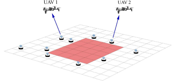
Figure 3: Multiple UAVs serve limited-power sensors to minimize power expenditure while also minimizing the age of information for data retrieval from the sensors. The environment is characterized by a riskier region for navigation of the UAVs in the middle of the grid world (colored area).

Consider a grid world, as shown in Fig. 3, where each cell is a square of length $L_{c}$. The system comprises a set $\mathcal{M}$ of $M$ uplink IoT devices deployed uniformly in the grid world. The devices report their observations to $I$ fixed-velocity rotary-wing UAVs flying at height $h$ and starting from positions selected randomly on the grid. The grid world contains normal cells, represented as white squares, and a risk region of special cells, colored in the figure. Whenever UAVs cross the risk region, there is a chance of failure, e.g., due to a higher collision probability. The current position at each time $t$ of each UAV $i$ is projected on the plane as coordinates $\left(x^{i}_{t},y^{i}_{t}\right)$. The DT monitoring of this system aims to determine trajectories for the UAVs on the grid that jointly minimize the AoI and the transmission powers across all the IoT devices.

The AoI measures the freshness of the information collected by the UAVs from the devices [42]. For each device $m$, the AoI is defined as the time elapsed since the last time data from the device was collected by a UAV [43, 44]. Accordingly, the AoI of device $m$ at time $t$ is updated as follows

$$A_{t}^{m}=\begin{cases}1,&\quad\text{if}\ V_{t}^{m}=1,\\ \text{min}\{A_{\rm max},A_{t-1}^{m}+1\},&\quad\text{otherwise};\end{cases}$$ (27)

where $A_{\rm max}$ is the maximum AoI, and $V_{t}^{m}=1$ indicates that device $m$ is served by a UAV at time step $t$. The maximum value $A_{\rm max}$ determines the maximum penalty assigned to the UAVs for not collecting data from a device at any given time.

For the sake of demonstrating the idea, we assume line-of-sight (LoS) communication links and write the channel gain between agent $i$ and device $m$ at time step $t$ as

$$g_{t}^{i,m}=\frac{g_{0}}{h^{2}+(L_{t}^{i,m})^{2}},$$ (28)

where $g_{0}$ is the channel gain at a reference distance of $1$ m and $L_{t}^{i,m}$ is the distance between UAV $i$ and device $m$ at time $t$. Using the standard Shannon capacity formula, for device $m$ to communicate to UAV $i$ at time step $t$, the transmission power must be set to [45]

$$P_{t}^{i,m} =\frac{\left(2^{\frac{E}{B}}\!-1\right)\sigma^{2}}{g_{t}^{i,m}},$$ (29)

where $E$ is the size of the transmitted packet, $B$ is the bandwidth, and $\sigma^{2}$ is the noise power.

If all the UAVs are outside the risk region, the reward function is given deterministically as a weighted combination of the sums of AoI and powers across all agents

$$r_{t}=-\frac{1}{M}\sum_{m=1}^{M}A_{t}^{m}-\lambda\sum_{m=1}^{M}P_{t}^{i_{m},m},$$ (30)

where $\lambda>0$ is a parameter that controls the desired trade-off between AoI and power consumption. In contrast, if any of the UAVs is within the risk region, with probability $p_{\mathrm{risk}}$, the reward is given by (30) with the addition of a penalty value $\mathrm{P_{\mathrm{risk}}}>0$, while it is equal to (30) otherwise.

To complete the setting description, we define state and actions as follows. The global state of the system at each time step $t$ is the collection of the UAVs’ positions and the individual AoI of the devices, i.e., $s_{t}=\left[x_{t}^{1},y_{t}^{1},\cdots,x_{t}^{I},y_{t}^{I},A_{t}^{1},A_{t}^{2},\cdots,A_{t}^{M}\right]$. At each time $t$, the action $a_{t}^{i}=[w_{t}^{i},d_{t}^{i}]$ of each UAV $i$ includes the direction $w^{i}_{t}\in\{\text{north},\text{south},\text{east},\text{west},\text{hover}\}$, where “hover” represents the decision of staying in the same cell, while the other actions move the UAV by one cell in the given direction. It also includes the identity $d_{t}^{i}\in\mathcal{M}\cup\{0\}$ of the device served at time $t$, with $d_{t}^{i}=0$ indicating that no device is served by UAV $i$.

VI-B Implementation and Dataset Collection

TABLE III: Simulation parameters and hyperparameters

Parameter	Value	Parameter	Value
$g_{0}$	$30$ dB	$\alpha$	$1$
$B$	$1$ MHz	$\gamma$	$0.99$
$h$	$100$ m	$\xi$	$0.15$
$E$	$5$ Mb	$\sigma^{2}$	$-100$ dBm
$\gamma$	$0.99$	$A_{\max}$	100
Batch size	$128$	$\lambda$	$500$
Iterations $K$	$150$	$p_{\mathrm{risk}}$	0.1
$L_{c}$	$100$ m	Optimizer	Adam

We consider a $10\times 10$ grid world with $I=2$ UAVs serving $M=10$ limited-power sensors and a $5\times 4$ risk region in the middle of the grid world as illustrated in Fig. 3. We use a fully connected neural network with two hidden layers of size $256$ and ReLU activation functions to represent the Q-function and the quantiles. The experiments are implemented using Pytorch on a single NVIDIA Tesla V100 GPU. Table III shows the UAV network parameters and the proposed schemes’ hyperparameters. We compare the proposed method MA-CQR to baseline offline MARL schemes, namely MA-DQN [46], MA-CQL (see Sec.IV-A), and MA-QR-DQN. MA-DQN corresponds to MA-CQL when no conservative penalty for OOD is applied, i.e., $\alpha=0$ in (15), whereas MA-QR-DQN corresponds to MA-CQR when $\alpha=0$ and $\xi=1$. Both the independent and centralized training frameworks apply to MA-DQN and MA-QR-DQN.

For the proposed MA-CQR, we consider two settings for the risk tolerance level $\xi$, namely $\xi=1$ and $\xi=0.15$, with the former corresponding to a risk-neutral design. We refer to the former as MA-CQR and the latter as MA-CQR-CVaR. For all distributional RL schemes (MA-QR-DQN and MA-CQR in all its variants), the learning rate is set to $10^{-5}$, while for all other schemes, we use a learning rate of $10^{-4}$.

The offline dataset $\mathcal{D}$ is collected using online independent DQN agents. In particular, we train the UAVs using an online MA-DQN algorithm until convergence and use $6\%$ and $16\%$ of the total number of transitions from the observed experience as the offline datasets.

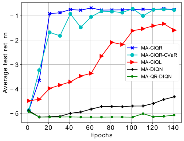
Figure 4: Average test return as a function of the number of training epochs at the DT using $\mathrm{P_{risk}}=100$ and $16\%$ offline dataset for a system of $2$ UAVs serving $10$ sensors. The return is averaged over $100$ test episodes at the end of each training epoch and shown upon division by $1000$.

VI-C Numerical Results

First, we show the simulation results of the proposed model via independent Q-learning compared to the baseline schemes. Then, we investigate the benefits of the CTDE approach compared to independent training.

VI-C1 Independent Learning

Fig. 4 shows the average test return, evaluated online using $100$ test episodes, for the policies obtained after a given number of training epochs at the DT. The figure thus reports the actual return obtained by the system as a function of the computational load at the DT, which increases with the number of training epochs.

We first observe that both MA-DIQN and MA-QR-DIQN, designed for online learning, fail to converge in the offline setting at hand. This well-known problem arises from overestimating Q-values corresponding to OOD actions in the offline dataset [10]. In contrast, conservative strategies designed for offline learning, namely MA-CIQL, MA-CIQR, and MA-CIQR-CVaR, exhibit an increasing average return as a function of the training epochs. In particular, the proposed MA-CIQR and MA-CIQR-CVaR provide the fastest convergence, needing around $30$ training epochs to reach the maximum return. In contrast, MA-CIQL shows slower convergence. This highlights the benefits of distributional RL in handling the inherent uncertainties arising in multi-agent systems from the environment and the actions of other agents [11].

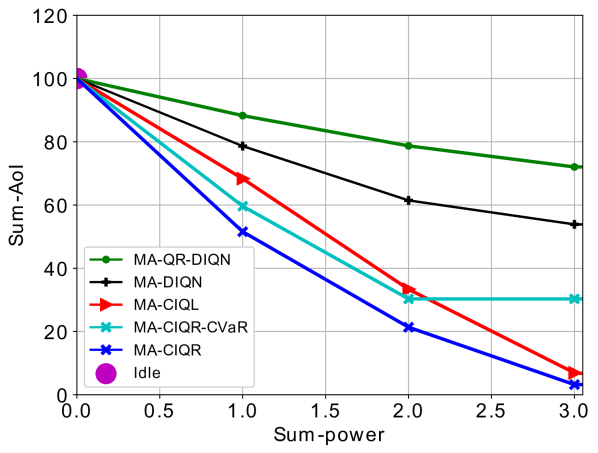
Figure 5: Sum-AoI as a function of the sum-power using $\mathrm{P_{risk}}={\lambda}/{4}$ and $16\%$ offline dataset for a system of $2$ UAVs serving $10$ sensors.

In Fig 5, we report the optimal achievable trade-off between sum-AoI and sum-power consumption across the devices. This region is obtained by training the different schemes while sweeping the hyperparameter values $\lambda$. We recall that the hyperparameter $\lambda$ controls the weight of the power as compared to the AoI in the reward function (30). In particular, setting $\lambda\rightarrow 0$ minimizes the AoI only, resulting in a round-robin optimal policy. At the other extreme, setting a large value of $\lambda$ causes the UAV never to probe the devices, achieving the minimum power equal to zero, and the maximum AoI $A_{\max}=100$. This point is denoted as “idle point” the figure. The other curves represent the minimum sum-AoI achievable as a function of the sum-power.

From Fig. 5, we observe that the proposed MA-CIQR always achieves the best age-power trade-off with the least age and sum-power consumption within al the curves. As in Fig. 4, MA-DIQN and MA-QR-DIQN provide the worst performance due to their failure to handle the uncertainty arising from OOD actions.

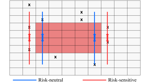
Figure 6: A comparison between the trajectories of two UAVs using risk-neutral and risk-sensitive policies obtained via MA-CIQR and MA-CIQR-CVaR, respectively. Crosses represent the positions of the devices.

In the next experiment, we investigate the capacity of the proposed risk-sensitive scheme MA-CIQR-CVaR to avoid risky trajectories. As a first illustration of this aspect, Fig. 6 shows two examples of trajectories obtained via MA-CIQR and MA-CIQR-CVaR. It is observed that the risk-neutral policies obtained by MA-CIQR take shortcuts through the risky area, while the risk-sensitive trajectories obtained via MA-CIQR-CVaR avoid entering the risky area.

VI-C2 Centralized Learning

Here, we compare the centralized training approach with independent learning. Fig. 7 shows the average test return as a function of training epochs for an environment of $2$ agents and $10$ sensors. We use two offline datasets with different sizes, equal to $6\%$ and $16\%$ of the total transitions from the observed experience of online DQN agents. We increase the value of the risk region penalty to $\mathrm{P_{risk}}=300$ compared to the previous subsection experiments.

Fig. 7a elucidates that the performance of the independent learning schemes is affected by increasing the risk penalty $\mathrm{P_{risk}}$. Specifically, MA-CIQL fails to reach convergence, while MA-CIQR and MA-CIQR-CVaR reach near-optimal performance but with a slower and less stable convergence than their centralized variants. However, as in Fig. 7b, a significant performance gap is observed between the proposed independent schemes and their centralized counterpart for reduced dataset size. This illustrates the merits of the CTDE approach in coordinating between agents during training, requiring less data to obtain effective policies.

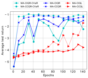
(a) $16\%$ dataset size

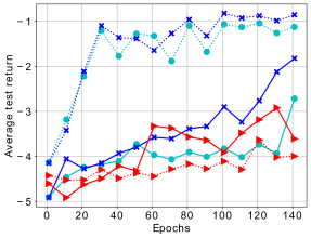
(b) $6\%$ dataset size

Figure 7: Average test return as a function of the number of training epochs at the DT for penalty $\mathrm{P_{risk}}=300$ in a system of $3$ UAVs and $15$ sensors with data set size equal to (a) $16\%$ and (b) $6\%$. The return is averaged over $100$ test episodes at the end of each training epoch, and shown upon division by $1000$.

In a manner similar to Fig. 5, Fig. 8 shows the trade-off between sum-AoI and sum-power consumption for both independent and centralized training approaches for a system of $3$ agents serving $15$ sensors. Increasing the parameter $\lambda$ in (30) reduces the total power consumption at the expense of AoI. Here again, we observe a significant gain in performance for MA-CCQR and MA-CCQR-CVaR compared to their independent variants. In contrast, the non-distributional schemes, MA-CIQL and MA-CCQL, show similar results, as both perform poorly in this low data regime.

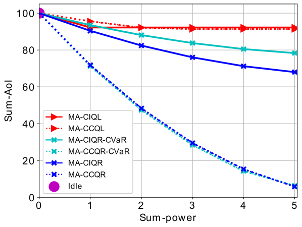
Figure 8: Sum-AoI as a function of the sum-power for penalty $\mathrm{P_{risk}}={\lambda}/{2.5}$ in a system of $3$ UAVs and $15$ sensors (data set size equal to $6\%$).

Finally, to gain further insights into the comparison between MA-CCQR and MA-CCQR-CVaR, we leverage two metrics as in [23], namely the percentage of violations and the $\text{CVaR}_{0.15}$ return. The former is the percentage of timesteps at which one of the UAVs enters the risk region with respect to the total number of timesteps. In contrast, the $\text{CVaR}_{0.15}$ metric is the average return of the 15% worst episodes.

In Table IV, we report these two metrics, as well as the average return, with all returns normalized by 1000. Thanks to the ability of MA-CCQR-CVaR to learn how to avoid the risk region, this scheme has the lowest percentage of violations among all the schemes. In addition, it achieves the largest $\text{CVaR}_{0.15}$ return, with a small gain in terms of average return as compared to MA-CCQR. This demonstrates the advantages of the risk-sensitive design of policies.

TABLE IV: Performance evaluation over $100$ test episodes after $150$ training iterations for penalty $\mathrm{P_{risk}}={\lambda}/{2.5}$ in a system of $3$ UAVs and $15$ sensors (data set size equal to $6\%$).

Algorithm	Average return	$\text{CVaR}_{0.15}$ return	Violations
MA-DQN (online)	$-1.5633$	$-1.9611$	$11.83\%$
MA-DCQN	$-4.8993$	$-5.4930$	$8.29\%$
MA-QR-DCQN	$-4.2987$	$-4.5743$	$6.85\%$
MA-CCQL	$-3.8518$	$-4.4695$	$17.7\%$
MA-CCQR	$-1.4028$	$-2.1775$	$8.56\%$
MA-CCQR-CVaR	$\boldsymbol{-1.3641}$	$\boldsymbol{-1.8513}$	$\boldsymbol{5.83\%}$

VII Conclusions

In this paper, we developed a distributional and conservative offline MARL scheme for DT-based wireless systems. We considered optimizing the CVaR of the cumulative return to obtain risk-sensitive policies. We introduce two variants of the proposed scheme depending on the level of coordination between the agents during training. The proposed algorithms were applied to the trajectory optimization problem in UAV networks. Numerical results illustrate that the learned policies avoid risky trajectories more effectively and yield the best performance compared to the baseline MARL schemes. The proposed approach can be extended by considering online fine-tuning of the policies in the PT to handle the possible changes in the deployment environment compared to the one generating the offline dataset.

References

- [1] A. Lavin, D. Krakauer, H. Zenil, J. Gottschlich, T. Mattson, J. Brehmer, A. Anandkumar, S. Choudry, K. Rocki, A. G. Baydin et al., “Simulation intelligence: Towards a new generation of scientific methods,” arXiv preprint arXiv:2112.03235, 2021.
- [2] R. Saracco, “Digital twins: Bridging physical space and cyberspace,” Computer, vol. 52, no. 12, pp. 58–64, 2019.
- [3] M. Raza, P. M. Kumar, D. V. Hung, W. Davis, H. Nguyen, and R. Trestian, “A digital twin framework for industry 4.0 enabling next-gen manufacturing,” in 2020 9th international conference on industrial technology and management (ICITM). IEEE, 2020, pp. 73–77.
- [4] P. Coveney and R. Highfield, Virtual You: How Building Your Digital Twin Will Revolutionize Medicine and Change Your Life. Princeton University Press, 2023.
- [5] L. U. Khan, W. Saad, D. Niyato, Z. Han, and C. S. Hong, “Digital-twin-enabled 6g: Vision, architectural trends, and future directions,” IEEE Communications Magazine, vol. 60, no. 1, pp. 74–80, 2022.
- [6] J. Mirzaei, I. Abualhaol, and G. Poitau, “Network digital twin for open RAN: The key enablers, standardization, and use cases,” arXiv preprint arXiv:2308.02644, 2023.
- [7] D. Villa, M. Tehrani-Moayyed, C. P. Robinson, L. Bonati, P. Johari, M. Polese, S. Basagni, and T. Melodia, “Colosseum as a digital twin: Bridging real-world experimentation and wireless network emulation,” arXiv preprint arXiv:2303.17063, 2023.
- [8] J. Zheng, T. H. Luan, Y. Zhang, R. Li, Y. Hui, L. Gao, and M. Dong, “Data synchronization in vehicular digital twin network: A game theoretic approach,” IEEE Transactions on Wireless Communications, 2023.
- [9] S. V. Albrecht, F. Christianos, and L. Schäfer, Multi-Agent Reinforcement Learning: Foundations and Modern Approaches. MIT Press, 2024. [Online]. Available: https://www.marl-book.com
- [10] S. Levine, A. Kumar, G. Tucker, and J. Fu, “Offline reinforcement learning: Tutorial, review, and perspectives on open problems,” arXiv preprint arXiv:2005.01643, 2020.
- [11] M. G. Bellemare, W. Dabney, and M. Rowland, Distributional Reinforcement Learning. MIT Press, 2023, http://www.distributional-rl.org.
- [12] A. Kumar, A. Zhou, G. Tucker, and S. Levine, “Conservative Q-learning for offline reinforcement learning,” Advances in Neural Information Processing Systems, vol. 33, pp. 1179–1191, 2020.
- [13] M. A. Abd-Elmagid, A. Ferdowsi, H. S. Dhillon, and W. Saad, “Deep reinforcement learning for minimizing age-of-information in UAV-assisted networks,” in 2019 IEEE Global Communications Conference (GLOBECOM). IEEE, 2019, pp. 1–6.
- [14] M. Samir, C. Assi, S. Sharafeddine, D. Ebrahimi, and A. Ghrayeb, “Age of information aware trajectory planning of UAVs in intelligent transportation systems: A deep learning approach,” IEEE Transactions on Vehicular Technology, vol. 69, no. 11, pp. 12 382–12 395, 2020.
- [15] E. Eldeeb, J. M. de Souza Sant’Ana, D. E. Pérez, M. Shehab, N. H. Mahmood, and H. Alves, “Multi-UAV path learning for age and power optimization in IoT with UAV battery recharge,” IEEE Transactions on Vehicular Technology, vol. 72, no. 4, pp. 5356–5360, 2022.
- [16] K. Ciosek, “Imitation learning by reinforcement learning,” in International Conference on Learning Representations, 2022. [Online]. Available: https://openreview.net/forum?id=1zwleytEpYx
- [17] J. Schulman, S. Levine, P. Abbeel, M. Jordan, and P. Moritz, “Trust region policy optimization,” in International conference on machine learning. PMLR, 2015, pp. 1889–1897.
- [18] M. G. Bellemare, W. Dabney, and R. Munos, “A distributional perspective on reinforcement learning,” in International conference on machine learning. PMLR, 2017, pp. 449–458.
- [19] W. Dabney, M. Rowland, M. Bellemare, and R. Munos, “Distributional reinforcement learning with quantile regression,” in Proceedings of the AAAI Conference on Artificial Intelligence, vol. 32, no. 1, 2018.
- [20] W. Dabney, G. Ostrovski, D. Silver, and R. Munos, “Implicit quantile networks for distributional reinforcement learning,” in International conference on machine learning. PMLR, 2018, pp. 1096–1105.
- [21] R. T. Rockafellar, S. Uryasev et al., “Optimization of conditional value-at-risk,” Journal of risk, vol. 2, pp. 21–42, 2000.
- [22] S. H. Lim and I. Malik, “Distributional reinforcement learning for risk-sensitive policies,” Advances in Neural Information Processing Systems, vol. 35, pp. 30 977–30 989, 2022.
- [23] Y. Ma, D. Jayaraman, and O. Bastani, “Conservative offline distributional reinforcement learning,” Advances in Neural Information Processing Systems, vol. 34, pp. 19 235–19 247, 2021.
- [24] J. Jiang and Z. Lu, “Offline decentralized multi-agent reinforcement learning,” 2023.
- [25] L. Pan, L. Huang, T. Ma, and H. Xu, “Plan better amid conservatism: Offline multi-agent reinforcement learning with actor rectification,” in International Conference on Machine Learning. PMLR, 2022, pp. 17 221–17 237.
- [26] J. Shao, Y. Qu, C. Chen, H. Zhang, and X. Ji, “Counterfactual conservative Q learning for offline multi-agent reinforcement learning,” 2023.
- [27] X. Wang, H. Xu, Y. Zheng, and X. Zhan, “Offline multi-agent reinforcement learning with implicit global-to-local value regularization,” arXiv preprint arXiv:2307.11620, 2023.
- [28] Y. Yang, X. Ma, C. Li, Z. Zheng, Q. Zhang, G. Huang, J. Yang, and Q. Zhao, “Believe what you see: Implicit constraint approach for offline multi-agent reinforcement learning,” 2021.
- [29] K. Yang, C. Shen, J. Yang, S. ping Yeh, and J. Sydir, “Offline reinforcement learning for wireless network optimization with mixture datasets,” 2023.
- [30] E. Eldeeb, M. Shehab, and H. Alves, “Traffic learning and proactive UAV trajectory planning for data uplink in markovian IoT models,” 2023.
- [31] F. Wu, H. Zhang, J. Wu, L. Song, Z. Han, and H. V. Poor, “AoI minimization for UAV-to-device underlay communication by multi-agent deep reinforcement learning,” in GLOBECOM 2020 - 2020 IEEE Global Communications Conference, 2020, pp. 1–6.
- [32] J. Cui, Y. Liu, and A. Nallanathan, “Multi-agent reinforcement learning-based resource allocation for UAV networks,” IEEE Transactions on Wireless Communications, vol. 19, no. 2, pp. 729–743, 2020.
- [33] Y. S. Nasir and D. Guo, “Multi-agent deep reinforcement learning for dynamic power allocation in wireless networks,” IEEE Journal on Selected Areas in Communications, vol. 37, no. 10, pp. 2239–2250, 2019.
- [34] N. Naderializadeh, J. J. Sydir, M. Simsek, and H. Nikopour, “Resource management in wireless networks via multi-agent deep reinforcement learning,” IEEE Transactions on Wireless Communications, vol. 20, no. 6, pp. 3507–3523, 2021.
- [35] Q. Zhang, W. Saad, and M. Bennis, “Millimeter wave communications with an intelligent reflector: Performance optimization and distributional reinforcement learning,” IEEE Transactions on Wireless Communications, vol. 21, no. 3, pp. 1836–1850, 2021.
- [36] ——, “Distributional reinforcement learning for mmwave communications with intelligent reflectors on a uav,” in GLOBECOM 2020-2020 IEEE Global Communications Conference. IEEE, 2020, pp. 1–6.
- [37] Y. Hua, R. Li, Z. Zhao, X. Chen, and H. Zhang, “Gan-powered deep distributional reinforcement learning for resource management in network slicing,” IEEE Journal on Selected Areas in Communications, vol. 38, no. 2, pp. 334–349, 2019.
- [38] P. Sunehag, G. Lever, A. Gruslys, W. M. Czarnecki, V. Zambaldi, M. Jaderberg, M. Lanctot, N. Sonnerat, J. Z. Leibo, K. Tuyls et al., “Value-decomposition networks for cooperative multi-agent learning,” arXiv preprint arXiv:1706.05296, 2017.
- [39] R. Lowe, Y. Wu, A. Tamar, J. Harb, P. Abbeel, and I. Mordatch, “Multi-agent actor-critic for mixed cooperative-competitive environments,” 2020.
- [40] R. Bellman, “Dynamic programming,” Science, vol. 153, no. 3731, pp. 34–37, 1966.
- [41] H. Xu, L. Jiang, J. Li, Z. Yang, Z. Wang, V. W. K. Chan, and X. Zhan, “Offline RL with no OOD actions: In-sample learning via implicit value regularization,” 2023.
- [42] E. Eldeeb, D. E. Pérez, J. Michel de Souza Sant’Ana, M. Shehab, N. H. Mahmood, H. Alves, and M. Latva-Aho, “A learning-based trajectory planning of multiple UAVs for AoI minimization in IoT networks,” in 2022 Joint European Conference on Networks and Communications & 6G Summit (EuCNC/6G Summit), 2022, pp. 172–177.
- [43] E. Eldeeb, M. Shehab, A. E. Kalø r, P. Popovski, and H. Alves, “Traffic prediction and fast uplink for hidden markov iot models,” IEEE Internet of Things Journal, vol. 9, no. 18, pp. 17 172–17 184, 2022.
- [44] A. Kosta, N. Pappas, and V. Angelakis, “Age of information: A new concept, metric, and tool,” Foundations and Trends in Networking, Now Publishers, Inc., 2017.
- [45] E. Eldeeb, M. Shehab, and H. Alves, “Age minimization in massive iot via uav swarm: A multi-agent reinforcement learning approach,” in 2023 IEEE 34th Annual International Symposium on Personal, Indoor and Mobile Radio Communications (PIMRC), 2023, pp. 1–6.
- [46] A. Tampuu, T. Matiisen, D. Kodelja, I. Kuzovkin, K. Korjus, J. Aru, J. Aru, and R. Vicente, “Multiagent cooperation and competition with deep reinforcement learning,” PloS one, vol. 12, no. 4, p. e0172395, 2017.