Effective refractive index of a silicon dioxide with
implanted Ag nanoparticles and Er³⁺ ions

Abstract

We consider light propagation in a silicon dioxide substrate with implanted ${\mathrm{Er}}^{3+}$ ions and silver nanoparticles that are randomly and homogeneously distributed in the substrate. When their densities are large enough, the medium can have a negative refractive index over a certain range of frequencies, within which the following exotic property ensues: increasing the electric and magnetic plasma frequencies, the medium transparency is augmented.

I Introduction

Negative refraction (NR) is a phenomenon in which electromagnetic waves are refracted at an interface of a material with a refraction angle that is negative relative to commonly observed refraction angles [1, 2, 3, 4, 5]. It was believed that, in order for NR to occur at a given frequency, the real part of the (electric) permittivity ($\varepsilon$) and real part of the (magnetic) permeability ($\mu$) must both be negative at this particular frequency [1, 2, 3, 4, 5, 6, 7, 8, 9]. Such materials are sometimes called “double negative” materials. NR meta-materials, i.e., specially designed NR materials made from assemblies of multiple elements fashioned from composite materials have been developed [3, 6, 7, 8, 9]. Moreover, it has often been stated that light at frequencies such that ${\mathrm{Re}}[\varepsilon(\omega)]{\mathrm{Re}}[\mu(\omega)]<0$ {i.e., ${\mathrm{Re}}[\varepsilon(\omega)]>0$ and ${\mathrm{Re}}[\mu(\omega)]<0$ or {${\mathrm{Re}}[\varepsilon(\omega)]<0$ and ${\mathrm{Re}}[\mu(\omega)]>0$} is not able to propagate in materials [1, 2, 3, 4, 5, 6, 7, 8, 9]; these are simplistic interpretations based upon the assumption that the permittivity and permittivity are real functions of frequency. Reference [10] is an exception; it used the amplitude-phase representation of the permittivity, permeability and refractive index. It considers two resultant complex refractive indices, $n(\omega)=\pm\sqrt{\varepsilon(\omega)\mu(\omega)/(\varepsilon_{0}\mu_{0})}$. While the resultant complex refractive index $n(\omega)$ with the minus sign is not a physical solution, because it gives negative absorption (i.e., gain), the refractive index $n(\omega)$ with the plus sign has the right properties. Recently, Ref. [11] considered negative refraction in achiral materials using the Drude model, and chiral materials using the Drude-Born-Fedorov model. That paper shows that the time-averaged Poynting vector always points along the wave vector, the time-averaged energy flux density is always positive, and the time-averaged energy density is positive (negative) when the refractive index is positive (negative). The phase velocity is negative when the real part of the refractive index is negative, and the group velocity generally changes sign several times as a function of frequency near resonance.

Here we study the optical properties a silicon dioxide substrate doped with silver nanoparticles and Er³⁺ ions. The electric permittivity of silver is negative over a wide frequency range, and Er³⁺ ions have a magnetic dipole optical transition from the ground state to the first excited state with a transition frequency of $\omega_{0}=2\pi\times 194$ THz [12]. Therefore, SiO₂ doped with silver and erbium can exhibit a negative refractive index in a frequency range just above $\omega_{0}$, and the width of the range depends on a number density of silver nanoparticles and a number density of erbium ions. Outside this frequency range, the imaginary part of the complex refractive index is much larger than the real part, and light cannot propagate in the medium. We also study the propagation of light from vacuum into the medium through an interface. When the refractive index is negative, the medium is transparent and the reflection coefficient is small. If the refractive index is positive, the reflection coefficient is close to unity, and the light is reflected from the interface.

NR materials are man-made meta-materials. NR meta-materials have led to significant technological advancements [4, 5, 6, 7, 8, 9] including: (1) superlensing, i.e., overcoming the diffraction limit of conventional lenses, allowing for sub-wavelength imaging for high-resolution microscopy [13, 14], (2) cloaking using devices that can manipulate the flow of light around an object, rendering it invisible to observers [4, 15, 16], (3) terahertz imaging, spectroscopy, and communication systems, enabling non-invasive inspections in biomedical imaging and security screening [17], (4) antennas incorporating NR meta-materials that can enhance the radiated power of the antenna NR by focusing electromagnetic radiation by a flat lens versus dispersion [18, 19, 20]. Note that there has been one report of a naturally occurring NR material, the Dirac semi-metal Cd₃As₂ [21].

The manuscript is organized as follows. Section II describes a medium consisting of a SiO₂ substrate doped with Ag nanoparticles and Er³⁺ ions. In Sec. III, we calculate the complex permittivity $\varepsilon_{\mathrm{eff}}(\omega)$ of SiO₂ with implanted silver nanoparticles, and show that the real part $\varepsilon^{\prime}_{\mathrm{eff}}(\omega)$ is negative over a wide frequency interval. In Sec. IV, we calculate the complex permeability $\mu_{\mathrm{Er}}(\omega)$ of Er³⁺ ions implanted into the SiO₂ substrate, and show that there is a frequency interval wherein its real part $\mu^{\prime}_{\mathrm{Er}}(\omega)<0$. In Sec. V, we calculate the complex refractive index $n_{\mathrm{eff}}(\omega)$ of the SiO₂ substrate with Ag nanoparticles and Er³⁺ ions, and show that $n^{\prime}_{\mathrm{eff}}(\omega)$ can be positive or negative depending on the sign of $\mu^{\prime}_{\mathrm{Er}}(\omega)$. In Sec. VI we discuss the position-dependence of the electric and magnetic fields inside the sample for $\omega_{\pm}=\omega_{0}\pm 2\pi\times 50~{}\text{kHz}$ and show that for $\omega=\omega_{+}$, $n^{\prime}_{\mathrm{eff}}(\omega_{+})<0$, and the imaginary part, $n^{\prime\prime}_{\mathrm{eff}}(\omega)$ is small, $n^{\prime\prime}_{\mathrm{eff}}(\omega_{+})\ll|n^{\prime}_{\mathrm{eff}}(\omega_{+})|$. Therefore the electromagnetic fields propagate with very small absorption (the medium is almost transparent for light with the frequency $\omega_{+}$), but for $\omega=\omega_{-}$, $n^{\prime}_{\mathrm{eff}}(\omega_{-})$ is positive and $n^{\prime}_{\mathrm{eff}}(\omega_{-})\ll n^{\prime\prime}_{\mathrm{eff}}(\omega)$, hence the electromagnetic fields are strongly reflected and decrease exponentially near the edge of the medium. In Sec. VII, we consider light propagating in a vacuum and impinging on the interface separating the vacuum and the medium, and show that the medium is transparent for light with $\omega=\omega_{+}$ where the real part of the refractive index is negative. However, for $\omega_{-}<\omega_{0}$, $n^{\prime}_{\mathrm{eff}}(\omega)>0$, and the light is reflected from the interface.

II SiO₂ substrate doped with $\text{Er}^{3+}$ ions and Silver nanoparticles

Doping silicon dioxide (SiO₂) with impurities can change its optical properties. References [22, 23] consider a silicon dioxide substrate doped with silver nanoparticles. A variety of shapes of the silver nanoparticles are possible, such as triangular, pentagonal, prolate, spheres, rods, cubes and prisms [22]. The size of the nanoparticles can range from one nanometer to hundreds of nanometers [22]. Reference [12] studies Er³⁺ ions implanted in a SiO₂ substrate. Er³⁺ doped zinc phosphate glasses containing spherical Ag nanoparticles with diameter in the range of 20-40 nm were synthesized in Ref. [24].

Here we theoretically analyze the optical properties of a SiO₂ substrate with implanted silver nanoparticles and Er³⁺ ions, as schematically shown in Fig. 1, when it is subject to a ray of light of wavelenght $\lambda$. The nanoparticles, assumed to have the same size and shape are randomly and homogeneously distributed in the substrate, as are the ions [25]. The nanoparticle size, the averaged distance between the neighboring nanoparticles, and between the ions are much smaller than $\lambda$ so we can parametrize the medium by an effective complex permittivity and permeability. We will focus our attention on light frequencies just above the resonance frequency $\omega_{0}=2\pi\times 194$ THz of the magnetic dipole transition in Er³⁺ ions [12]. This reference showed that when the density of the Er³⁺ ions is high enough, the real part of the permeability is negative over a certain frequency region, and when the density of the Ag nanoparticles is high enough, the real part of the permittivity can be negative. Hence, the medium can have a negative refractive index.

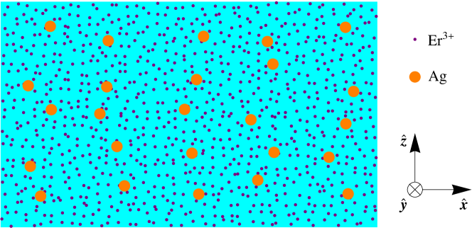
Figure 1: Silicon dioxide substrate (aqua) with implanted Er³⁺ ions (purple) and silver nanoparticles (Ag, orange) localized at random locations within the substrate. The Cartesian basis vectors are $\hat{\mathbf{x}}$, $\hat{\mathbf{y}}$ and $\hat{\mathbf{z}}$. Note that $N_{\mathrm{Er}^{+}}>N_{\mathrm{Ag}}$.

III Effective permittivity of silver nanoparticles

In Gaussian units, the permittivity of silver is calculated using the Drude model [26],

$$\varepsilon_{\mathrm{Ag}}(\omega)=\varepsilon_{\infty}-\frac{\omega_{p,e}^{2}}{\omega^{2}+i\omega\gamma_{\mathrm{Ag}}},$$ (1)

where $\varepsilon_{\infty}=5\pm 2$ is the background permittivity, $\gamma_{\mathrm{Ag}}=(60\pm 8)\times 10^{12}~{}\text{s}^{-1}$ is the width (the inverse mean free lifetime) of the permittivity, and $\omega_{p,e}=(13.5\pm 0.3)\times 10^{15}~{}\text{s}^{-1}$ is the plasma frequency [26]. The silver and silicon dioxide permeabilities are $\mu_{\mathrm{Ag}}=\mu_{\rm SiO_{2}}=1$. We calculate the effective permittivity of silver nanoparticles doped into SiO₂ substrate assuming the silver nanoparticles have spherical shape of radius $r_{0}=40$ nm.

When a nanoparticle of radius $r_{0}$ is placed in an external electric field $\bm{\mathcal{E}}(t)=\bm{\mathcal{E}}_{0}\,e^{-i\omega t}$, the induced dipole momentum is

$$\mathbf{p}(t)=\frac{4\pi}{3}\,r_{0}^{3}\,\big{(}\varepsilon_{\mathrm{Ag}}(\omega)-1\big{)}\,\bm{\mathcal{E}}(t)\equiv\alpha(\omega)\bm{\mathcal{E}}(t).$$ (2)

The polarizability $\alpha(\omega)$ of a single nanoparticle is related to the effective permittivity $\varepsilon_{\mathrm{eff}}(\omega)$ of a set of nanoparticles with number density $N_{\mathrm{Ag}}$ by the Lorentz-Lorenz formula,

$$\frac{\varepsilon_{\mathrm{eff}}(\omega)-\varepsilon_{\rm SiO_{2}}(\omega)}{\varepsilon_{\mathrm{eff}}(\omega)+2\varepsilon_{\rm SiO_{2}}(\omega)}=\frac{4\pi N_{\mathrm{Ag}}\alpha(\omega)}{3},$$ (3)

which can also be written as the Clausius-Mossotti relation,

$$\varepsilon_{\mathrm{eff}}(\omega)=\varepsilon_{\rm SiO_{2}}(\omega)\,\frac{\displaystyle 1+2\,\Big{(}\frac{4\pi}{3}\Big{)}^{2}\,N_{\mathrm{Ag}}r_{0}^{3}\,\big{[}\varepsilon_{\mathrm{Ag}}(\omega)-1\big{]}}{\displaystyle 1-\Big{(}\frac{4\pi}{3}\Big{)}^{2}\,N_{\mathrm{Ag}}r_{0}^{3}\,\big{[}\varepsilon_{\mathrm{Ag}}(\omega)-1\big{]}}.$$ (4)

When the nanoparticle density vanishes, $N_{\mathrm{Ag}}r_{0}^{3}\to 0$, $\varepsilon_{\mathrm{eff}}(\omega)$ reduces to the SiO₂ permittivity $\varepsilon_{\rm SiO_{2}}(\omega)$. For $\omega_{+}=\omega_{0}+2\pi\times 50$ kHz, where $\omega_{0}=2\pi\times 194$ THz, $\varepsilon_{\rm SiO_{2}}(\omega_{+})=2.37$ is real and positive. When $N_{\mathrm{Ag}}r_{0}^{3}\neq 0$, $\varepsilon_{\mathrm{eff}}(\omega)$ is complex, and the imaginary part is positive and proportional to $\mathrm{Im}[\varepsilon_{\mathrm{Ag}}(\omega)]$. There is a value of the dimensionless parameter $\mathcal{N}=N_{\mathrm{Ag}}r_{0}^{3}$, $\mathcal{N}_{c}=0.0002405$, such that for $\mathcal{N}<\mathcal{N}_{c}$, $\mathrm{Re}[\varepsilon_{\mathrm{eff}}(\omega_{+})]>0$, and for $\mathcal{N}>\mathcal{N}_{c}$, $\mathrm{Re}[\varepsilon_{\mathrm{eff}}(\omega_{+})]<0$. Note that for $N_{\mathrm{Ag}}r_{0}^{3}=\mathcal{N}_{c}$, the average distance between the neighboring nanoparticles, $N_{\mathrm{Ag}}^{-1/3}=16.08\,r_{0}$ is much larger than $r_{0}$. Here we take $\mathcal{N}=8\mathcal{N}_{c}$, for which

$$\varepsilon_{\mathrm{eff}}(\omega_{+})=-3.322+0.058\,i.$$ (5)

Figure 2 shows the real and imaginary parts of the permittivity, $\varepsilon^{\prime}_{\mathrm{eff}}(\omega)$ and $\varepsilon^{\prime\prime}_{\mathrm{eff}}(\omega)$, versus $\omega$. There is a density dependent threshold frequency $\omega_{\mathrm{th}}(\mathcal{N})$ such that $\varepsilon^{\prime}_{\mathrm{eff}}(\omega)<0$ for $\omega<\omega_{\mathrm{th}}(\mathcal{N})$, and $\varepsilon^{\prime}_{\mathrm{eff}}(\omega)>0$ for $\omega>\omega_{\mathrm{th}}(\mathcal{N})$. In Fig. 2(a), $\omega_{\mathrm{th}}(\mathcal{N})$ is the frequency where $\varepsilon^{\prime}_{\mathrm{eff}}(\omega_{\mathrm{th}}(\mathcal{N}))=0$. Note that $\varepsilon^{\prime\prime}_{\mathrm{eff}}(\omega)\geq 0$ for all $\omega\geq 0$.

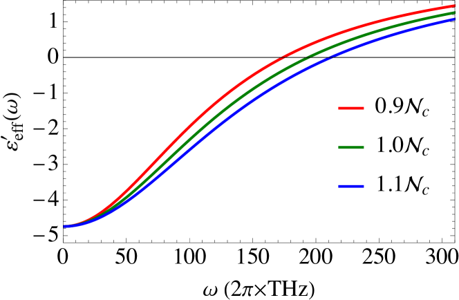
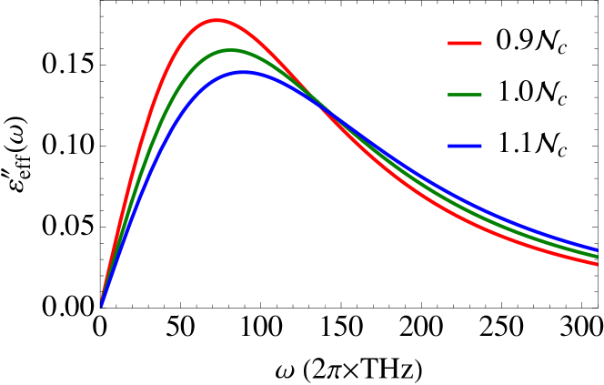
Figure 2: Real and imaginary parts, $\varepsilon^{\prime}_{\mathrm{eff}}(\omega)$ and $\varepsilon^{\prime\prime}_{\mathrm{eff}}(\omega)$, of the permittivity of SiO₂ doped with silver nanoparticles versus $\omega$ for a several values of $\mathcal{N}$.

IV Relative permeability of the ions

The lowest-energy states of Er³⁺ ions, ordered from the lowest up, have $L=6$, $S=\frac{3}{2}$ and $J=\frac{15}{2},\frac{13}{2},\frac{11}{2},\frac{9}{2}$ [12]. The magnetic dipole transition from the ground state $J=15/2$ to the excited state $J^{\prime}=13/2$ has frequency $\omega_{0}=2\pi\times 194$ THz.

The magnetic susceptibility can be calculated using a Drude formula (see Appendix B for details):

$$\chi_{\mathrm{Er}}(\omega)=-\frac{N_{\mathrm{Er}}\mu_{B}^{2}\omega_{0}}{5\hbar}\,\frac{1}{\omega^{2}-\omega_{0}^{2}+i\gamma_{\mathrm{Er}}\omega},$$ (6)

where $N_{\mathrm{Er}}$ is the number density of ions, and $\gamma_{\mathrm{Er}}$ is the line-width of the ${}^{4}I_{15/2}$–${}^{4}I_{13/2}$ magnetic dipole transition. The nomenclature for spectral terms ${}^{4}I_{J}$ for Er³⁺ ions is clarified in Appendix A. The lifetime of Er³⁺ ions implanted in a bulk SiO₂ substrate is $\gamma_{\mathrm{Er}}^{-1}=(14.3\pm 0.3)^{-1}$ ms [12], hence $\gamma_{\mathrm{Er}}=(70\pm 1)~{}\text{s}^{-1}$. Equation (6) is derived in Appendix B.

The permeability of Er³⁺, $\mu_{\mathrm{Er}}(\omega)=1+4\pi\chi_{\mathrm{Er}}(\omega)$ is

$$\mu_{\mathrm{Er}}(\omega)=1-\frac{\omega_{p,m}^{2}}{\omega^{2}-\omega_{0}^{2}+i\gamma_{\mathrm{Er}}\omega},$$ (7)

where the magnetic plasma frequency is

$$\omega_{p,m}^{2}=\frac{4\pi N_{\mathrm{Er}}\mu_{B}^{2}\,\omega_{0}}{5\hbar}.$$ (8)

The real part of the permeability, $\mu^{\prime}_{\mathrm{Er}}(\omega)$, has a minimum at $\omega_{\min}=\sqrt{\omega_{0}(\omega_{0}+\gamma_{\mathrm{Er}})}$,

$$\mu^{\prime}_{\mathrm{Er}}(\omega_{\min})=1-\frac{\omega_{p,m}^{2}}{\gamma_{\mathrm{Er}}(2\omega_{0}+\gamma_{\mathrm{Er}})}.$$

For $\omega_{p,m}>\sqrt{\gamma_{\mathrm{Er}}(2\omega_{0}+\gamma_{\mathrm{Er}})}=2\pi\times 6.56\times 10^{7}$ Hz, $\mu^{\prime}_{\mathrm{Er}}(\omega_{\min})$ is negative. Hereafter, we take $N_{\mathrm{Er}}=10^{19}~{}\text{cm}^{-3}$, and $\omega_{p,m}=2\pi\times 7.96\times 10^{9}$ Hz. The real part of the permeability is negative for $\omega_{0}<\omega<\sqrt{\omega_{0}^{2}+\omega_{p,m}^{2}}$, where $\sqrt{\omega_{0}^{2}+\omega_{p,m}^{2}}-\omega_{0}=2\pi\times 163$ kHz. For $\omega=\omega_{+}$,

$$\mu_{\mathrm{Er}}(\omega_{+})=-2.26+0.00036\,i.$$ (9)

Figure 3 shows the real part, $\mu^{\prime}_{\mathrm{Er}}(\omega)$, and the imaginary part, $\mu^{\prime\prime}_{\mathrm{Er}}(\omega)$, of the permeability versus $\omega$. For $\omega_{0}<\omega<\omega_{0}+2\pi\times 163$ kHz, $\mu^{\prime}_{\mathrm{Er}}(\omega)<0$, otherwise $\mu^{\prime}_{\mathrm{Er}}(\omega)>0$. Figure 3(b) shows the permeability near the $M_{1}$ resonance frequency $\omega_{0}$.

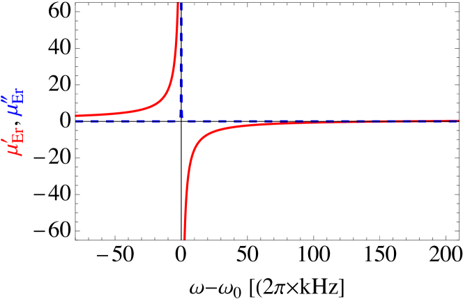
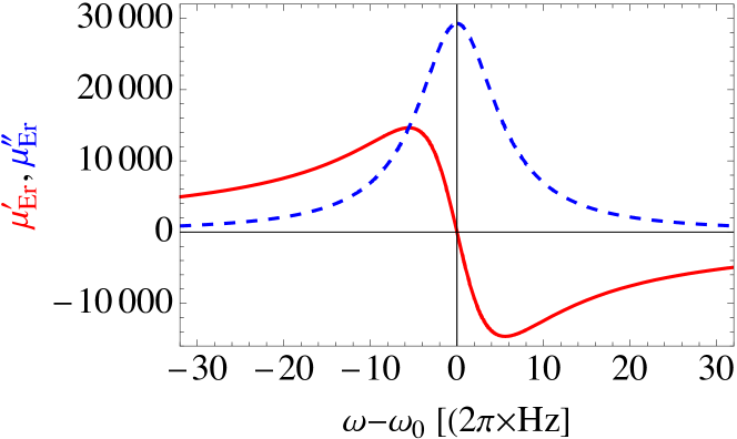
Figure 3: (a) Real (solid red) and imaginary (dashed blue) parts of the permeability, $\mu^{\prime}_{\mathrm{Er}}(\omega)$ and $\mu^{\prime\prime}_{\mathrm{Er}}(\omega)$, of SiO₂ doped with Er³⁺ ions, versus $\omega$ for $N_{\mathrm{Er}}=1\times 10^{19}~{}\text{cm}^{-3}$. (b) Zoom of the frequency region near $\omega_{0}$.

V Refractive index

The refractive index $n_{\mathrm{eff}}(\omega)$ of a SiO₂ substrate implanted with Ag nanoparticles and Er³⁺ ions is given by

$$n_{\mathrm{eff}}(\omega)=\sqrt{\varepsilon_{\mathrm{eff}}(\omega)\,\mu_{\mathrm{Er}}(\omega)}\,.$$ (10)

In Eq. (10), it is convenient to write $\varepsilon_{\mathrm{eff}}(\omega)$ [see Eq. (4)] and $\mu_{\mathrm{Er}}(\omega)$ [see Eq. (7)] as

$$\varepsilon_{\mathrm{eff}}(\omega) = |\varepsilon_{\mathrm{eff}}(\omega)|\,e^{i\theta_{\varepsilon}(\omega)},$$

$$\mu_{\mathrm{Er}}(\omega) = |\mu_{\mathrm{Er}}(\omega)|\,e^{i\theta_{\mu}(\omega)}.$$

For $\omega=\omega_{+}$, $|\varepsilon_{\mathrm{eff}}(\omega_{+})|=3.322$, $|\mu_{\mathrm{Er}}(\omega_{+})|=2.262$, $\theta_{\varepsilon}(\omega_{+})=\pi-0.017$ and $\theta_{\mu}(\omega_{+})=\pi-0.00016$, hence $n_{\mathrm{eff}}(\omega_{+})$ is

$$n_{\mathrm{eff}}(\omega_{+}) = \sqrt{|\varepsilon_{\mathrm{eff}}(\omega_{+})|\,|\mu_{\mathrm{Er}}(\omega_{+})|}\,e^{i[\theta_{\varepsilon}(\omega_{+})+\theta_{\mu}(\omega_{+})]/2}$$ (11)

$$\approx \sqrt{|\varepsilon_{\mathrm{eff}}(\omega_{+})|\,|\mu_{\mathrm{Er}}(\omega_{+})|}\,\times$$

$$\bigg{\{}-1+\frac{i[2\pi-\theta_{\varepsilon}(\omega_{+})+\theta_{\mu}(\omega_{+})]}{2}\bigg{\}}.\quad$$

Numerically, $n_{\mathrm{eff}}(\omega_{+})=-2.741+0.024\,i$. Note that the real part $n^{\prime}_{\mathrm{eff}}(\omega_{+})$ of the refractive index is negative. The imaginary part $n^{\prime\prime}_{\mathrm{eff}}(\omega_{+})$ is very small, hence the medium is optically transparent.

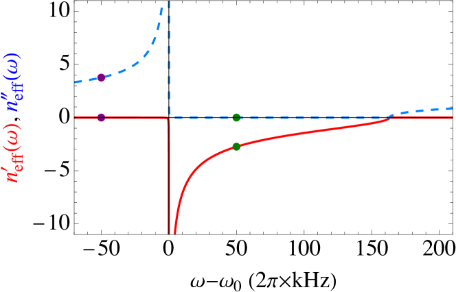
Figure 4: For $N_{\mathrm{Ag}}=3.002\times 10^{13}~{}\text{cm}^{-3}$ and $N_{\mathrm{Er}}=1.0\times 10^{19}~{}\text{cm}^{-3}$, the figure shows the real part (solid red) and the imaginary part (dashed blue) of the refractive index in Eq. (10). The purple dot is for $n_{\mathrm{eff}}(\omega_{-})$ and the green dot is for $n_{\mathrm{eff}}(\omega_{+})$.

The complex refractive index plotted as a function of frequency is shown in Fig. 4. For $\omega<\omega_{0}$, $\mathrm{Im}[n_{\mathrm{eff}}(\omega)]\gg\mathrm{Re}[n_{\mathrm{eff}}(\omega)]$ and the medium is not transparent. For $\omega_{0}<\omega<\omega_{1}=\omega_{0}+2\pi\times 163.1~{}\text{kHz}$, $\mathrm{Re}[n_{\mathrm{eff}}(\omega)]<0$ and $\mathrm{Im}[n_{\mathrm{eff}}(\omega)]\ll 1$, hence the medium is transparent for this frequency interval. For $\omega>\omega_{1}$, the medium is not transparent.

We consider here two additional cases:

• $N_{\mathrm{Ag}}\neq 0$, and $N_{\mathrm{Er}}=0$;

• $N_{\mathrm{Ag}}=0$, and $N_{\mathrm{Er}}\neq 0$.

For $N_{\mathrm{Er}}=0$, the permeability is $\mu=1$, and the refractive index $n_{\varepsilon}(\omega_{+})$ is

$$n_{\varepsilon}(\omega_{+}) = \sqrt{|\varepsilon_{\mathrm{eff}}(\omega_{+})|}\,e^{\frac{i}{2}\theta_{\varepsilon}(\omega_{+})}$$ (12)

$$= 0.016+1.823\,i.$$

Note that the imaginary part of $n_{\varepsilon}(\omega_{+})$ is large, hence the SiO₂ substrate with implanted Ag nanoparticles is not transparent.

For $N_{\mathrm{Ag}}=0$, the permittivity $\varepsilon_{\rm SiO_{2}}(\omega_{+})$ is real and positive, and the refractive index $n_{\mu}(\omega_{+})$ is

$$n_{\mu}(\omega_{+}) = \sqrt{\varepsilon_{\rm SiO_{2}}(\omega_{+})\,|\mu_{\mathrm{Er}}(\omega_{+})|}\,e^{\frac{i}{2}\,\theta_{\mu}(\omega_{+})}$$ (13)

$$= 0.00019+2.316\,i.$$

As in the former case, the imaginary part of $n_{\mu}(\omega_{+})$ is large, hence the SiO₂ substrate with implanted Er³⁺ ions is not transparent. But the imaginary part of $n_{\mathrm{eff}}(\omega)$ is very small. How is it possible that upon implanting Ag nanoparticles and the Er³⁺ ions into the SiO₂ substrate, the medium is optically transparent? We will answer this question in Sec. VII, but first we consider the spatial dependence of the electric, magnetic, polarization and magnetization fields inside the sample.

VI Space and time dependence of the fields

In this section we describe the dependence on $\mathbf{r}$ and $t$ of the electric and displacement fields $\mathbf{E}(\mathbf{r},t)$, $\mathbf{D}(\mathbf{r},t)$, as well as the magnetic, magnetic induction, magnetization and polarization fields, $\mathbf{H}(\mathbf{r},t)$, $\mathbf{B}(\mathbf{r},t)$, $\mathbf{M}(\mathbf{r},t)$, $\mathbf{P}(\mathbf{r},t)$. Specifically, we consider the cases where the real parts of the permittivity and permeability are positive and negative, respectively.

Consider light with frequency $\omega$ propagating along the $z$-axis and polarized along the $x$-axis. The light wave number is $k\,n_{\mathrm{eff}}(\omega)$, where $k=\omega/c$ is the wave number in vacuum. The complex electric field of the light is

$$\bm{\mathcal{E}}(z,t)=E_{0}\,e^{i[n_{\mathrm{eff}}(\omega)kz-\omega t]}\,\hat{\mathbf{x}},$$ (14a)

where $$E_{0}$$ is assumed to be real and positive. The complex displacement and polarization fields are

$$\bm{\mathcal{D}}(z,t) = \varepsilon_{\mathrm{eff}}(\omega)\,E_{0}\,e^{i[n_{\mathrm{eff}}(\omega)kz-\omega t]}\,\hat{\mathbf{x}},$$ (14b)

$$\bm{\mathcal{P}}(z,t) = \frac{\varepsilon_{\mathrm{eff}}(\omega)-1}{4\pi}\,E_{0}\,e^{i[n_{\mathrm{eff}}(\omega)kz-\omega t]}\,\hat{\mathbf{x}}.$$ (14c)

Applying Faraday’s induction law, we find the complex induction magnetic field,

$$\bm{\mathcal{B}}(z,t)=n_{\mathrm{eff}}(\omega)\,E_{0}\,e^{i[n_{\mathrm{eff}}(\omega)kz-\omega t]}\,\hat{\mathbf{y}}.$$ (14d)

The complex magnetic and magnetization fields are

$$\bm{\mathcal{H}}(z,t)=\eta(\omega)\,E_{0}\,e^{i[n_{\mathrm{eff}}(\omega)kz-\omega t]}\,\hat{\mathbf{y}},$$ (14e)

$$\bm{\mathcal{M}}(z,t)=\frac{\mu_{\mathrm{Er}}(\omega)-1}{4\pi}\,\eta(\omega)\,E_{0}\,e^{i[n_{\mathrm{eff}}(\omega)kz-\omega t]}\,\hat{\mathbf{y}}.\quad$$ (14f)

Here we write the permittivity and permeability as $\varepsilon_{\mathrm{eff}}(\omega)=|\varepsilon_{\mathrm{eff}}(\omega)|\,e^{i\theta_{\varepsilon}}$ and $\mu_{\mathrm{Er}}(\omega)=|\mu_{\mathrm{Er}}(\omega)|\,e^{i\theta_{\mu}}$, and define $\eta(\omega)$ as

$$\eta(\omega)=\sqrt{\frac{|\varepsilon_{\mathrm{eff}}(\omega)|}{|\mu_{\mathrm{Er}}(\omega)|}}\,e^{i\theta_{\eta}},$$ (15)

where $\theta_{\eta}=\frac{1}{2}\,[\theta_{\varepsilon}-\theta_{\mu}]$. The physical fields $\mathbf{E}(z,t)$, $\mathbf{D}(z,t)$, $\mathbf{P}(z,t)$, $\mathbf{B}(z,t)$, $\mathbf{H}(z,t)$ and $\mathbf{M}(z,t)$ are the real parts of the complex fields specified in Eq. (14).

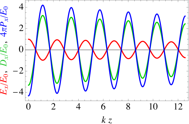
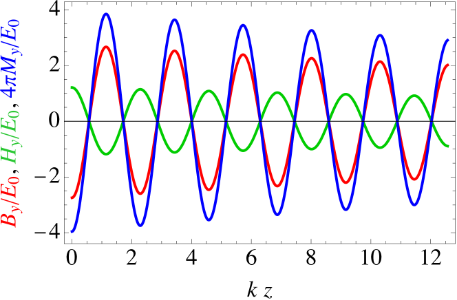
Figure 5: (a) The spatial dependence of the fields $\mathbf{E}(z,0)$ [red], $\mathbf{D}(z,0)$ [green] and $4\pi\mathbf{P}(z,0)$ [blue], and (b) the fields $\mathbf{B}(z,0)$ [red], $\mathbf{H}(z,0)$ [green] and ${\color[rgb]{0,0,1}4\pi}\mathbf{M}(z,0)$ [blue] for $\omega=\omega_{+}$ where the real parts of the permittivity and permeability are negative.

The spatial dependence of the fields shown in Fig. 5 are for $\omega=\omega_{+}$, where the real parts of the permittivity and permeability are negative. Figure 5 shows that $\mathbf{E}(z,0)$ [red] is opposite to $\mathbf{D}(z,0)$ [green] and $\mathbf{P}(z,0)$ [blue]. This is because $\mathrm{Re}[\varepsilon_{\mathrm{eff}}(\omega)]<-1$, and $\mathrm{Im}[\varepsilon_{\mathrm{eff}}(\omega)]$ is small. Figure 5 shows that $\mathbf{H}(z,0)$ [green] is opposite to $\mathbf{B}(z,0)$ [red] and $\mathbf{M}(z,0)$ [blue], since $\mathrm{Re}[\mu_{\mathrm{Er}}(\omega)]<-1$ and $\mathrm{Im}[\mu_{\mathrm{Er}}(\omega)]$ is small. $\mathrm{Im}[\mu_{\mathrm{Er}}(\omega)]$ increases when the frequency approaches the resonance frequency $\omega_{0}$, and $\mathbf{H}(z,0)$ and $\mathbf{M}(z,0)$ get a phase shift due to the imaginary part of the permittivity.

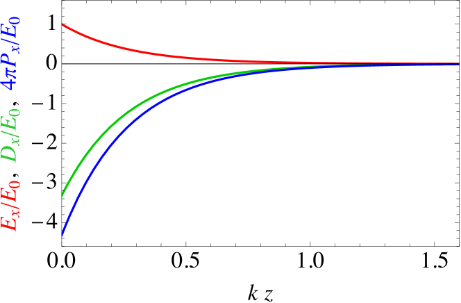
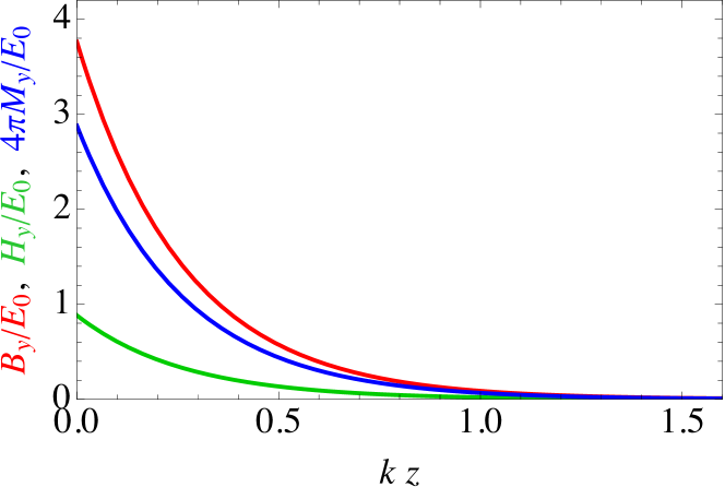
Figure 6: (a) The fields $\mathbf{E}(z,0)$ [red], $\mathbf{D}(z,0)$ [green] and $4\pi\mathbf{P}(z,0)$ [blue]. (b) the fields $\mathbf{B}(z,T/4)$ [red], $\mathbf{H}(z,T/4)$ [green] and ${\color[rgb]{0,0,1}4\pi}\mathbf{M}(z,T/4)$ [blue] for $\omega=\omega_{-}$ where the real parts of the permittivity is negative and real part of permeability is positive. Here $T=2\pi/\omega$.

The fields are shown in Fig. 6 for $\omega_{-}=\omega_{0}-2\pi\times 50~{}\text{kHz}$, where the real part of the permittivity is negative and the real part of the permeability is positive. Figure 6 shows that $\mathbf{E}(z,0)$ [red] is opposite to $\mathbf{D}(z,0)$ [green] and $\mathbf{P}(z,0)$ [blue], since $\mathrm{Re}[\varepsilon_{\mathrm{eff}}(\omega)]<-1$, and $\mathrm{Im}[\varepsilon_{\mathrm{eff}}(\omega)]$ is small. The real part of the refractive index is much smaller than the imaginary part, hence the fields exponentially vanish with $z$. Figure 6 shows the fields $\mathbf{B}(z,T/4)$, $\mathbf{H}(z,T/4)$ and $4\pi\mathbf{M}(z,T/4)$, where $T=2\pi/\omega$. Since $\mathrm{Im}[n_{\mathrm{eff}}(\omega)]\gg\mathrm{Re}[n_{\mathrm{eff}}(\omega)]$, the fields are very small at $t=0$. The fields decrease with $z$ and vanish for $z\to\infty$. Therefore the light with $\omega<\omega_{0}$ cannot propagate in the medium. When we have an interface separating the medium and the vacuum, the light is reflected from the interface.

VII Light reflection from the interface between the vacuum and medium

Consider light with frequency $\omega$ propagating in vacuum and impinges on a planar interface (in the $x-y$ plane) between vacuum and the medium with complex permittivity $\varepsilon_{\mathrm{eff}}(\omega)$, permeability $\mu_{\mathrm{Er}}(\omega)$ and refractive index $n_{\mathrm{eff}}(\omega)$. Let the light propagate along the $z$-direction which is perpendicular to the interface and polarized along the $x$-axis. The electric and magnetic fields in vacuum are

$$\bm{\mathcal{E}}_{\mathrm{vac}}(z,t) = \frac{1}{2}\,\Big{[}\mathcal{E}_{0}\,e^{ikz-i\omega t}+\mathcal{E}_{2}\,e^{-ikz-i\omega t}\Big{]}\hat{\mathbf{x}},$$ (16a)

$$\bm{\mathcal{H}}_{\mathrm{vac}}(z,t) = \frac{1}{2}\,\Big{[}\mathcal{E}_{0}\,e^{ikz-i\omega t}-\mathcal{E}_{2}\,e^{-ikz-i\omega t}\Big{]}\hat{\mathbf{y}},$$ (16b)

where $k=\omega/c$ is the wave-number of the light in vacuum, $\mathcal{E}_{0}$ is the real amplitude of the incident light and $\mathcal{E}_{2}$ is the complex amplitude of the reflected light. The electric and magnetic fields of the light in he medium are

$$\bm{\mathcal{E}}_{\mathrm{med}}(z,t) = \frac{1}{2}\,\mathcal{E}_{1}\,e^{in_{\mathrm{eff}}(\omega)\,kz-i\omega t}\,\hat{\mathbf{x}},$$ (17a)

$$\bm{\mathcal{H}}_{\mathrm{med}}(z,t) = \frac{1}{2}\,\frac{n_{\mathrm{eff}}(\omega)}{\mu_{\mathrm{Er}}(\omega)}\,\mathcal{E}_{1}\,e^{in_{\mathrm{eff}}(\omega)\,kz-i\omega t}\,\hat{\mathbf{y}},$$ (17b)

where $\mathcal{E}_{1}$ is the complex amplitude of the transmitted light. The electric and magnetic fields in Eqs. (16) and (17) satisfy the following boundary conditions at the interface $z=0$:

$$\bm{\mathcal{E}}_{\mathrm{vac}}(0,t) = \bm{\mathcal{E}}_{\mathrm{med}}(0,t),$$ (18a)

$$\bm{\mathcal{H}}_{\mathrm{vac}}(0,t) = \bm{\mathcal{H}}_{\mathrm{med}}(0,t),$$ (18b)

which imply

$$\mathcal{E}_{0}+\mathcal{E}_{2} = \mathcal{E}_{1},$$ (19a)

$$\mathcal{E}_{0}-\mathcal{E}_{2} = \eta(\omega)\,\mathcal{E}_{1}.$$ (19b)

Equations (19) imply

$$\mathcal{E}_{1} = \frac{2\mathcal{E}_{0}}{1+\eta(\omega)},$$ (20a)

$$\mathcal{E}_{2} = \mathcal{E}_{0}-\frac{2\eta(\omega)\,\mathcal{E}_{0}}{1+\eta(\omega)}.$$ (20b)

The energy flux (Poynting) vector of the electromagnetic field is $\mathbf{S}=\frac{c}{4\pi}\overline{\mathbf{E}\times\mathbf{H}}$, where the over-line means the temporal average, $\mathbf{E}=\tfrac{\bm{\mathcal{E}}+\bm{\mathcal{E}}^{*}}{2}$ and $\mathbf{H}=\tfrac{\bm{\mathcal{H}}+\bm{\mathcal{H}}^{*}}{2}$. The Poynting vector of the incident, transmitted and reflected light at $z=0$ are

$$S_{0}(0) = \frac{c}{8\pi}\,\mathcal{E}_{0}^{2},$$ (21a)

$$S_{1}(0) = \frac{c}{4\pi}\,\mathrm{Re}\big{[}\eta(\omega)\big{]}\,\big{|}\mathcal{E}_{1}\big{|}^{2},$$ (21b)

$$S_{2}(0) = \frac{c}{8\pi}\,\big{|}\mathcal{E}_{2}\big{|}^{2}.$$ (21c)

The reflection coefficient $\mathcal{R}(\omega)$ and the transmission coefficient $\mathcal{T}(\omega)$ are defined as

$$\mathcal{T}(\omega)=\frac{S_{1}(0)}{S_{0}(0)},\quad\mathcal{R}(\omega)=\frac{S_{2}(0)}{S_{0}(0)}.$$

Using Eqs. (21), we get

$$\mathcal{T}(\omega) = \frac{4\,\mathrm{Re}[\eta(\omega)]}{1+|\eta(\omega)|^{2}+2\mathrm{Re}[\eta(\omega)]},$$ (22)

$$\mathcal{R}(\omega) = \frac{1+|\eta(\omega)|^{2}-2\mathrm{Re}[\eta(\omega)]}{1+|\eta(\omega)|^{2}+2\mathrm{Re}[\eta(\omega)]}.$$ (23)

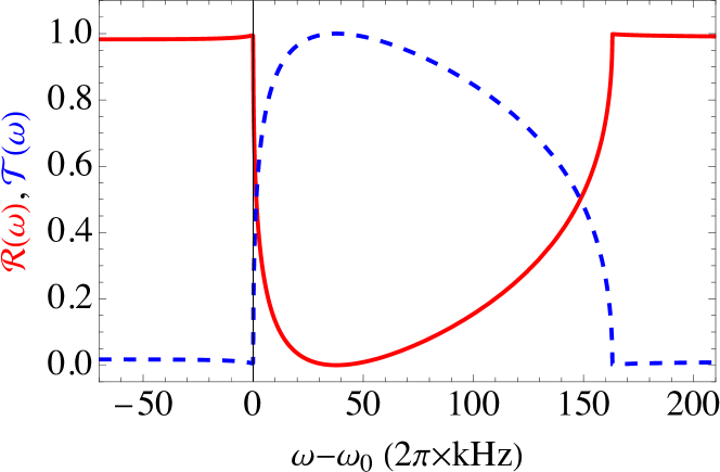
Figure 7: The reflection coefficient (solid red curve) and the transmission coefficient (dashed blue curve) versus frequency for $N_{\mathrm{Ag}}=3.002\times 10^{13}~{}\text{cm}^{-3}$ and $N_{\mathrm{Er}}=1\times 10^{19}~{}\text{cm}^{-3}$.

The reflection and transmission coefficients versus $\omega$ are shown in Fig. 7. For $\omega<\omega_{0}$, $\mathcal{R}(\omega)\approx 1$ and $\mathcal{T}(\omega)\ll 1$, hence almost all the light is reflected from the interface. For $\omega>\omega_{0}$, $\mathcal{R}(\omega)$ decreases and reaches its minimum, $\mathcal{R}(\omega_{\min})=1.855\times 10^{-5}$, at $\omega_{\min}=\omega_{0}+2\pi\times 37.74~{}\text{kHz}$. $\mathcal{R}(\omega)$ increases for $\omega>\omega_{\mathrm{min}}$. For $\omega=\omega_{+}$, $\mathcal{R}(\omega_{+})=0.009189$ is small.

VIII Summary and Conclusion

We calculated electric permittivity and magnetic permeability of SiO₂ with implanted Ag nanoparticles and Er³⁺ ions. We showed that when the number density of the nanoparticles and the number density of ions are larger than critical values, there is a frequency interval just above the $M_{1}$ transition frequency of Er³⁺ where the real part $n^{\prime}(\omega)$ of the complex refractive index $n(\omega)$ is negative, and the imaginary part $n^{\prime\prime}(\omega)$ is very small, see Fig. 4. Outside of this interval, $n^{\prime}(\omega)$ is much smaller than $n^{\prime\prime}(\omega)$. We also studied transmission and reflection of light from the interface separating vacuum and the medium. When the refractive index is negative, the medium is transparent and the reflection coefficient is small. When the refractive index is positive, the reflection coefficient is close to 1, and the light almost completely reflected from the interface. Hence the medium can be used as an infrared filter to selectively transmit light. We plan to generalize the theory to treat anisotropic crystals such as quartz and isotropic materials subject to a DC electric field.

Appendix A Spectral terms of atoms

The notation to denote the atomic energy levels (i.e., the spectral terms of the atoms or ions) is clarified in Ref. [28]: states with different values of the total angular momentum $L$ are denoted by capital Latin letters, as follows:

$$\begin{array}[]{cccccccccccccc}L&=&0&1&2&3&4&5&6&7&8&9&10&\ldots\\ &&S&P&D&F&G&H&I&K&L&M&N&\ldots\end{array}$$

Above and to the left of this letter is placed the number $2S+1$, called the multiplicity of the term, where $S$ is the total spin. When $L\geq S$, the number of fine-structure components is $2S+1$. Below and to the right of the letter is placed the value of the total orbital angular momentum $J$. Thus the symbols ${}^{4}I_{15/2}$ and ${}^{4}I_{13/2}$ denote the levels with $L=6$, $S=3/2$, $J=15/2$ and $13/2$.

Appendix B Derivation of the magnetic susceptibility in Eq. (6)

Interaction of an Er³⁺ ion with an alternating magnetic field, $\mathbf{B}(t)=\frac{1}{2}\mathbf{B}_{0}\,e^{-i\omega t}+\mathrm{c.c.}$, is given by the Hamiltonian

$$H_{\mathrm{dm}}=g_{L}\mu_{B}\,\mathbf{L}\cdot\mathbf{B}(t)+g_{S}\mu_{B}\,\mathbf{S}\cdot\mathbf{B}(t),$$ (24)

where $\mu_{B}$ is the Bohr magneton, $g_{L}\approx 1$ and $g_{S}\approx 2$ are the electron $g$-factors. $\mathbf{B}_{0}$ is assumed to be real and directed in the $z$ direction. For the frequency $\omega$ far detuned from the resonance frequency $\omega_{0}$, $H_{\mathrm{dm}}$ can be treated as a weak perturbation. The second order correction $\epsilon_{2}(m_{J},B_{0})$ to the ground-state energy due to the time-dependent interaction $H_{\mathrm{dm}}$ is

$$\epsilon_{2}(m_{J},B_{0}) = -\frac{\mu_{B}^{2}B_{0}^{2}}{4\hbar}\,\bigg{|}\Big{\langle}\frac{15}{2},m_{J}\Big{|}g_{L}L_{z}+g_{S}S_{z}\Big{|}\frac{13}{2},m_{J}\Big{\rangle}\bigg{|}^{2}$$ (25)

$$\times\bigg{[}\frac{1}{\omega_{0}-\omega-\frac{1}{2}\,i\gamma}+\frac{1}{\omega_{0}+\omega+\frac{1}{2}\,i\gamma}\bigg{]},$$

where $m_{J}$ is the projection of $\mathbf{J}$ on the $z$ axis, and $\gamma$ is the resonance width of the $J=\frac{15}{2}$ to $J^{\prime}=\frac{13}{2}$ quantum transition. Taking into account the equalities,

$$\Big{\langle}\frac{15}{2},m_{J}\Big{|}g_{L}L_{z}+g_{S}S_{z}\Big{|}\frac{13}{2},m_{J}\Big{\rangle}$$

$$\qquad\qquad=\big{(}g_{S}-g_{L}\big{)}\,\Big{\langle}\frac{15}{2},m_{J}\Big{|}S_{z}\Big{|}\frac{13}{2},m_{J}\Big{\rangle}$$

$$\qquad\qquad\approx\Big{\langle}\frac{15}{2},m_{J}\Big{|}S_{z}\Big{|}\frac{13}{2},m_{J}\Big{\rangle},$$

$$\frac{1}{\omega_{0}-\omega-\frac{1}{2}\,i\gamma}+\frac{1}{\omega_{0}+\omega+\frac{1}{2}\,i\gamma}\approx\frac{2\omega_{0}}{\omega_{0}^{2}-\omega^{2}-i\omega\gamma},$$

we can rewrite Eq. (25) as

$$\epsilon_{2}(m_{J},B_{0}) \approx -\frac{\mu_{B}^{2}B_{0}^{2}}{2\hbar}\,\frac{\omega_{0}}{\omega_{0}^{2}-\omega^{2}-i\omega\gamma}$$ (26)

$$\times\bigg{|}\Big{\langle}\frac{15}{2},m_{J}\Big{|}S_{z}\Big{|}\frac{13}{2},m_{J}\Big{\rangle}\bigg{|}^{2}.$$

The energy density $W_{2}(B_{0})$ of an ensemble of the Er³⁺ ions is

$$W_{2}(B_{0})=N_{\mathrm{Er}}\sum_{m_{J}}p_{m_{J}}\,\epsilon_{2}(m_{J},B_{0}),$$ (27)

where $N_{\mathrm{Er}}$ is the number density of the Er³⁺ ions, $p_{m_{J}}$ is the probability to find an ion is in the ground state with the magnetic number $m_{J}$, and

$$\sum_{m_{J}}p_{m_{J}}=1.$$

For equilibrium, $p_{m_{J}}=1/(2J+1)$ and we have

$$\frac{1}{2J+1}\sum_{m_{J}}\big{|}\langle L,S,J^{\prime},m_{J}|S_{z}|L,S,J,m_{J}\rangle\big{|}^{2}=\frac{2}{5},$$

where $J=\frac{15}{2}$ and $J^{\prime}=\frac{13}{2}$ on the left hand side of the equation.

Magnetic susceptibility $\chi_{\mathrm{Er}}(\omega)$ of the ensemble of the Er³⁺ ions is

$$\chi_{\mathrm{Er}}(\omega)=-\frac{\partial^{2}W_{2}(B_{0})}{\partial B_{0}^{2}}.$$ (28)

Substituting Eq. (27) into Eq. (28), we get

$$\chi_{\mathrm{Er}}(\omega) = -\frac{N\mu_{B}^{2}\omega_{0}}{2\hbar(\omega^{2}-\omega_{0}^{2}+i\gamma\omega)}\sum_{m_{J}}p_{m_{J}}$$ (29)

$$\times\big{|}\langle L,S,J^{\prime},m_{J}|S_{z}|L,S,J,m_{J}\rangle\big{|}^{2},$$

where $|L,S,J,m_{J}\rangle$ is the ground-state wave function with $L=6$, $S=3/2$ $J=15/2$, and the projection $m_{J}$ of the orbital angular momentum $\mathbf{J}$ on the $z$ axis,, $|L,S,J,m_{J}\rangle$ is the excited-state wave function with $J^{\prime}=13/2$, and $p_{m_{J}}$ is the probability to find an ion in the state $|L,S,J,m_{J}\rangle$. For equilibrium, Eq. (29) reduces to Eq. (6).

References

[1]
V. G. Veselago, “The electrodynamics of substances with simultaneously negative values of and ”. Soviet Physics Uspekhi 10, 509 (1968).
[2]
J. B. Pendry, D. R. Smith,
“Reversing Light With Negative Refraction”,
Physics Today 57, 37 (2004).
[3]
D. R. Smith, J. B. Pendry, M. C. K. Wiltshire,
“Metamaterials and Negative Refractive Index’,
Science 305, 788 (2004).
[4]
J. B. Pendry, D. Schurig, D. R. Smith,
“Controlling Electromagnetic Fields”,
Science 312, 1780 (2006).
[5]
V. Veselago, L. Braginsky, V. Shklover, C. Hafner,
“Negative Refractive Index Materials”,
J. Computat. Theor. Nanosci. 3, 1 (2006).
[6]
C. M. Krowne, Y. Zhang (Eds.), Physics of Negative Refraction and Negative Index Materials, (Springer, Berlin, 2007), see for example, p. 357, Fig. 12.15.
[7]
G. V. Eleftheriades, K. G. Balmain (Eds.), Negative-Refraction Metamaterials, Fundamental Principles and Applications, (John Wiley & Sons, Hoboken, 2005). See the paper by D. Schurig and D. R. Smith, “Negative Index Lenses”, Chapter 5, p. 221, after Eq. (5.15).
[8]
S. A. Ramakrishna, T. M. Grzegorczyk (Eds.), Physics and Applications of Negative Refractive Index Materials, (CRC Press, Boca Raton, 2009), see for example, p. 121, Fig. 3.21.
[9]
F. Capolino (Ed.), Theory and Phenomena of Metamaterials (CRC Press, Boca Raton, 2009). See for example the paper by C-W Qiu, S. Zouhdi and A. Sihvola, “A Review of Chiral and Bianisotropic Composite Materials Providing Backward Waves and Negative Refractive Indices”; Section 24.2 states: “In order to realize the negative refraction [16, 17], the composite material must have effective permittivity and permeability that are negative over the same frequency band. When the real parts of permittivity and permeability possess the same sign, the electromagnetic waves can propagate.”
[10]
M. W. McCall1,, A. Lakhtakia and W. S. Weiglhofer,
“The negative index of refraction demystified”,
Eur. J. Phys. 23 353 (2002).
[11]
Y. B. Band, I. Kuzmenko, M. Trippenbach,
“Negative Refraction in isotropic achiral and chiral materials”,
Phys. Rev. A (submitted), https://doi.org/10.48550/arXiv.2308.12019.
[12]
J. Bao, N. Yu, F. Capasso, T. Mates, M. Troccoli, and A. Belyanin,
“Controlled modification of erbium lifetime in silicon dioxide with metallic overlayers”,
Appl. Phys. Lett. 91, 131103 (2007).
[13]
J. B. Pendry,
“Negative Refraction Makes a Perfect Lens”,
Phys. Rev. Lett. 85, 3966 (2000).
[14]
X. Zhang, Z. Liu,
“Superlenses to overcome the diffraction limit”,
Nature Materials 7, 435 (2008).
[15]
U. Leonhardt, T. Philbin, Geometry and Light: The Science of Invisibility, Dover Books on Physics (Dover, 2010).
[16]
M. Kim and J. Rho, “Metamaterials and imaging”, Nano Convergence 2, (2015). DOI 10.1186/s40580-015-0053-7.
[17]
F. Ling, Z. Zhong, R. Huang and B. Zhang,
“A broadband tunable terahertz negative refractive index metamaterial”,
Sci. Rep. 8, 9843 (2018).
[18]
G. V. Eleftheriades, A. Grbic, and M. Antoniades,
“Negative-refractive-index metamaterials and enabling electromagnetic applications”,
Proc. IEEE Int. Symp. Antennas and Propagation 2, 1399-1402 (2004).
[19]
R. W. Ziolkowski and A. D. Kipple,
“Application of double negative materials to increase the power radiated by electrically small antennas”,
IEEE Trans Antennas and Propagation 51, 2626-2640, (2003).
[20] A. Rennings, S. Otto, C. Caloz, and P. Waldow,
“Enlarged half-wavelength resonator antenna with enhanced gain”,
Proc. IEEE Int. Symp. Antennas and Propagation 3A, 683 (2005).
[21]
C-Y Chen, M-C Hsu, C. D. Hu, Y C. Lin,
“Natural Negative-Refractive-Index Materials”,
Phys. Rev. Lett. 127, 237401 (2021).
[22]
V. Rentería-Tapia, C. Velásquez-Ordoñez,
M. Ojeda Martínez, E. Barrera-Calva, and
F. González-García,
“Silver nanoparticles dispersed on silica glass for
applications as photothermal selective material”,
Energy Procedia 57, 2241 ( 2014).
[23]
J. A. Badán, E. Navarrete-Astorga, R. Henríquez,
F. M. Jiménez, D. Ariosa, J. R. Ramos-Barrado, and
E. A. Dalchiele,
“Silver Nanoparticle Arrays onto Glass Substrates Obtained by
Solid-State Thermal Dewetting: A Morphological, Structural
and Surface Chemical Study”,
Nanomaterials 12, 617 (2022).
[24]
I. Soltani, S. Hraiech, K. Horchani-Naifer, H. Elhouichet, M. Férid,
“Effect of silver nanoparticles on spectroscopic properties of Er3+ doped phosphate glass”,
Optical Materials 46, 454 (2015).
[25]
Note that fluctuations in the density (and the size) of the Ag nanoparticles, and fluctuations of the ion density can result in a position-dependent fluctuation of the effective permittivity, permeability and refractive index which could cause some Rayleigh scattering loss, but we do not consider this here.
[26]
H. U. Yang, J. D’Archangel, M. L. Sundheimer, E. Tucker, G. D. Boreman, and M. B. Raschke,
“Optical dielectric function of silver”,
Phys. Rev. B 91, 235137 (2015).
[27]
P. Drude, Lehrbuchder Optik, (S.Hirzel, Leipzig, 1912).
[28]
L. D. Landau and E. M. Lifshitz,
Quantum Mechanics, Non-relativistic Theory,
vol. 3 of Course of Theoretical Physics.
(Pergamon Press, Oxford 1965),
p. 232.