SISSA 02/2024/FISI

We study a class of SYK models with $\mathcal{N}=2$ supersymmetry, described by $N$ fermions in chiral Fermi multiplets, as well as $\alpha N$ first-order bosons in chiral multiplets. The interactions are characterised by two integers $(p,q)$. We focus on the large $N$ and low energy limit of these models. Despite the presence of dynamical bosons, we find conformal behaviour akin to the standard SYK model. We use $\mathcal{I}$-extremization of a Witten index to study the supersymmetric solutions. In particular, we find an exact expression for the entropy, which matches the numerical solutions to the Schwinger–Dyson equations. We further solve the model both in the large $p$ and large $p,q$ limits. Numerically, we verify our analytical results and obtain estimates for the Schwarzian coupling in the near zero-temperature limit. We also study the low-lying spectrum of operators to determine the parameter ranges where the Schwarzian mode dominates the IR dynamics. Lastly, we study out-of-time-ordered correlators to show that the model is maximally chaotic.

1 Introduction and summary

The quantum-mechanical models introduced by Sachdev, Ye, and Kitaev (SYK) [1, 2] have the properties of being solvable at strong coupling in the large $N$ limit, exhibiting maximally chaotic behaviour, and developing an emergent conformal symmetry in the infrared (IR) [1, 3, 4, 2, 5, 6, 7]. Their IR physics is dominated by a pseudo Goldstone boson, the Schwarzian mode, which is dual to the two-dimensional JT gravity in AdS₂. Given the universal appearance of near-AdS₂ throats in the near-horizon region of near-extremal black holes, the SYK model poses itself as a model of quantum black-hole physics: it captures the dynamics of a universal “breathing” mode that lives in the near-horizon region [8, 9]. Many variations on the SYK model have been studied, including [10, 11, 12, 13, 14, 15, 16, 17, 18, 19, 20, 21, 22, 23, 24, 25, 26, 27, 28] which are close to the subject of this paper.

An interesting question is whether one can microscopically derive a certain type of SYK-like models directly from gravity or string theory [10]. A step in that direction was made in [29] in the context of holography and black holes in higher-dimensional AdS space. The quantum mechanical model found in [29] presents many peculiar features, e.g., it has $\mathcal{N}=2$ supersymmetry, it describes both dynamical fermions and bosons belonging to many species with unequal abundance in a large $N$ limit, it enjoys multiple Abelian symmetries.

With that motivation in mind, in this paper we study a class of SYK-like models with $\mathcal{N}=2$ supersymmetry, made of $N$ regular fermions in chiral Fermi multiplets, as well as $\alpha N$ bosons in chiral multiplets with one-derivative kinetic terms (a.k.a. first-order bosons), in the large $N$ limit. The parameter $\alpha$ controls the relative abundance. The interactions are described by “superpotential” $J$-terms (in the language of [30]), are controlled by two positive integers $(p,q)$ (where $p$ is odd), and may include — depending on $p,q$ — a scalar potential and Yukawa interactions. As in SYK, the interactions are all-to-all and given by random variables that represent quenched disorder.

Our model has some similarities to the $\mathcal{N}=2$ two-fermion model of [26]. Indeed our model has both a $U(1)_{R}$ R-symmetry and a $U(1)_{F}$ flavor symmetry, and we study the model with chemical potentials turned on, finding similar physical properties. We are particularly interested in the role played by dynamical bosons, which could lead to a variety of phenomena such as spin-glass phases or condensation, see e.g. [31, 32, 33, 34, 35, 28]. In our model, instead, bosons turn out to be tamed and lead to conformal solutions — both with and without supersymmetry — similarly to the standard SYK model. This implies that our $(p,q)$ models retain the main features expected from near-BPS black hole horizons, yet accommodating the presence of dynamical bosons, and make us confident that also the more convoluted, but also more realistic, quantum mechanical models of [29] might exhibit the same properties.

Let us summarize our results. In Section 2 we present our model. In Section 3 we solve the model in the annealed approximation and at leading order in $1/N$, in terms of Schwinger–Dyson equations. In particular we verify that the system admits both supersymmetric and non-supersymmetric conformal solutions in the IR. For certain values of the chemical potentials, we also find some non-conformal solutions in which the correlators behave as those of gapped free fields. Supersymmetric solutions at zero temperature can also be studied through a symmetry-refined Witten index. From it, employing $\mathcal{I}$-extremization [36, 37] we extract the zero-temperature entropy and the R-symmetry charge of the vacuum. Both are compatible with our numerical computations and with the Luttinger–Ward relation [38]. The entropy computation gives support to the claim that the model is conformal in the IR, rather than in a spin-glass phase. We analyse the system at large $p$, as well as at large $p$ and $q$. In these limits we are able to reach an intermediate low-energy regime which is conformal, but not the very low-energy behaviour, which is also conformal but with different spectrum. The two agree only in the supersymmetric case.

In Section 4 we perform various numerical analyses of our model, both for supersymmetric and non-supersymmetric values of the chemical potentials, for different values of $(p,q)$. In particular we solve the Schwinger–Dyson equations, confirming the IR conformal behaviour found analytically. We test the Luttinger–Ward relations and the computation of the zero-temperature entropy. Going to non-zero temperature allows us to extract the Schwarzian coupling.

In Section 5 we study the low-lying spectrum of operator dimensions. Besides observing the presence of the Schwarzian mode, the two currents, and their superpartners, we determine in which window of parameters we expect the Schwarzian mode to dominate the IR dynamics, and identify windows in which other modes are expected to dominate. In Section 6 we extract the Lyapunov exponents from the out-of-time-ordered (OTOC) 4-point functions, finding that the model is maximally chaotic (it saturates the bound of [39]).

We conclude in Section 7 by presenting a few puzzling results we hope to resolve in future work. We provide many appendices with the technical details of computations.

2 $\boldsymbol{\mathcal{N}=2}$ SYK models with dynamical bosons

We are interested in a quantum mechanical model with $\mathcal{N}=2$ supersymmetry (one complex supercharge) described by $N$ Fermi multiplets $\mathcal{Y}_{a}$ ($a=1,\dots,N$) and $\alpha N$ chiral multiplets $\Phi_{b}$ ($b=1,\dots,\alpha N$), where $\alpha$ is a positive real constant that we call the abundance parameter. The field content of a Fermi multiplet $\mathcal{Y}$ is a dynamical fermion $\eta$ and an auxiliary scalar $f$, while that of a chiral multiplet $\Phi$ is, in our model, a dynamical boson $\phi$ (with one-derivative kinetic term) and an auxiliary fermion $\psi$. In the Lagrangian formulation and in Lorentzian signature, the model is described by the action:

$$S_{\text{L}} =\int\!dt\,\biggl{[}i\eta_{a}^{\dagger}\bigl{(}\partial_{t}+i\mu_{\eta}\bigr{)}\eta_{a}+f_{a}^{\dagger}f_{a}+i\phi_{b}^{\dagger}\bigl{(}\partial_{t}+i\mu_{\phi}\bigr{)}\phi_{b}+\psi_{b}^{\dagger}\psi_{b}$$ (2.1)

$$\qquad\quad-J_{a_{1}\ldots a_{p}b_{1}\ldots b_{q}}\Bigl{(}p\,f_{a_{1}}\eta_{a_{2}}\cdots\eta_{a_{p}}\phi_{b_{1}}\cdots\phi_{b_{q}}+q\,\eta_{a_{1}}\cdots\eta_{a_{p}}\psi_{b_{1}}\phi_{b_{2}}\cdots\phi_{b_{q}}\Bigr{)}+\text{h.c.}\biggr{]}.$$

We use the convention that repeated indices are summed over. These so-called J-term interactions in the second line are inspired from the ones obtained in [29], corresponding here to the $p=1$, $q=2$ case. The couplings $J_{a_{1}\ldots a_{p}b_{1}\ldots b_{q}}$ are complex Gaussian random variables with zero mean and variance

$$\bigl{\langle}J^{\phantom{*}}_{a_{1}\ldots a_{p}b_{1}\ldots b_{q}}J^{*}_{c_{1}\ldots c_{p}d_{1}\ldots d_{q}}\bigr{\rangle}=\frac{J}{p\,q\,N^{p+q-1}}\,\delta_{a_{1}\ldots a_{p}}^{[c_{1}\ldots c_{p}]}\,\delta_{b_{1}\ldots b_{q}}^{(d_{1}\ldots d_{q})}\;.$$ (2.2)

Here $J$ has dimension of mass, and is kept fixed in the large $N$ limit so that the averaged partition function has uniform scaling. The couplings are antisymmetric in the first $p$ indices and symmetric in the next $q$ indices. Note that $p$ is odd, while $q$ is any positive integer. In (2.1) we have also included the chemical potentials $\mu_{\phi}$, $\mu_{\eta}$. Under charge conjugation

$$\eta_{a}\mapsto\eta_{a}^{\dagger}\;,\quad f_{a}\mapsto f_{a}^{\dagger}\;,\quad\phi_{b}\mapsto\phi_{b}^{\dagger}\;,\quad\psi_{b}\mapsto\psi_{b}^{\dagger}\;,\quad\mu_{\eta}\mapsto-\mu_{\eta}\;,\quad\mu_{\phi}\mapsto-\mu_{\phi}\;,$$ (2.3)

the Fermi multiplet kinetic terms are invariant, while the chiral multiplet kinetic terms are odd and thus they break charge conjugation symmetry.

Integrating out the auxiliary fields, the action becomes

$$S_{\text{L}} =\int\!dt\,\biggl{[}i\eta_{a}^{\dagger}\bigl{(}\partial_{t}+i\mu_{\eta}\bigr{)}\eta_{a}+i\phi_{b}^{\dagger}\bigl{(}\partial_{t}+i\mu_{\phi}\bigr{)}\phi_{b}$$ (2.4)

$$\qquad\quad-\Bigl{\lvert}p\,J_{a_{1}\ldots a_{p}b_{1}\ldots b_{q}}\eta_{a_{2}}\cdots\eta_{a_{p}}\phi_{b_{1}}\cdots\phi_{b_{q}}\Bigr{\rvert}^{2}-\Bigl{\lvert}q\,J_{a_{1}\ldots a_{p}b_{1}\ldots b_{q}}\eta_{a_{1}}\cdots\eta_{a_{p}}\phi_{b_{2}}\cdots\phi_{b_{q}}\Bigr{\rvert}^{2}\biggr{]}\,.$$

In the Hamiltonian formulation, the bosonic conjugate momentum to $\phi$ is $\Pi_{\phi}=i\phi^{\dagger}$ and therefore the (anti)commutation relations are $\{\eta_{a},\eta^{\dagger}_{c}\}=\delta_{ac}$ and $[\phi_{b},\phi^{\dagger}_{d}]=\delta_{bd}$ (all other ones vanishing). The Hamiltonian is $\widetilde{H}=H+\mu_{\eta}Q_{\eta}+\mu_{\phi}Q_{\phi}$, where

$$H=\bigl{\lvert}p\,J_{a_{1}\ldots a_{p}b_{1}\ldots b_{q}}\eta_{a_{2}}\cdots\eta_{a_{p}}\phi_{b_{1}}\cdots\phi_{b_{q}}\bigr{\rvert}^{2}+\bigl{\lvert}q\,J_{a_{1}\ldots a_{p}b_{1}\ldots b_{q}}\eta_{a_{1}}\cdots\eta_{a_{p}}\phi_{b_{2}}\cdots\phi_{b_{q}}\bigr{\rvert}^{2}$$ (2.5)

is the interacting Hamiltonian with chemical potentials turned off, while $Q_{\eta}=\frac{1}{2}[\eta_{a}^{\dagger},\eta_{a}]$ and $Q_{\phi}=\frac{1}{2}\{\phi_{b}^{\dagger},\phi_{b}\}$ are the charge operators. The ordering ambiguities in $H$ are fixed by supersymmetry by requiring that $H=\{\mathcal{Q},\mathcal{Q}^{\dagger}\}$ in terms of the supercharge

$$\mathcal{Q}\,\sim\,J_{a_{1}\ldots a_{p}b_{1}\ldots b_{q}}\eta_{a_{1}}\cdots\eta_{a_{p}}\phi_{b_{1}}\cdots\phi_{b_{q}}\;.$$ (2.6)

Each bosonic degree of freedom $\phi$ describes a particle in magnetic field (see, e.g., [40]). Upon canonical quantization, $Q_{\phi}\geq\frac{1}{2}$ and the bosonic Hilbert space is a Fock space with lowest weight state $|0\rangle$ defined by $\phi|0\rangle=0$ and generated by the creation operator $\phi^{\dagger}$. For $p=1$ the Hamiltonian $H$ includes a positive-definite scalar potential for $\phi$, and $\widetilde{H}$ is bounded from below for any given value of $\mu_{\phi}$ and finite $N$. However $J_{a_{1}\ldots a_{p}b_{1}\ldots b_{q}}$ goes to zero at large $N$, and thus one should take $\mu_{\phi}>0$ in order to avoid instabilities (as we will see, the limit $\mu_{\phi}\to 0$ is stable after taking the large $N$ limit). For $p>1$, $H$ has flat directions and thus one should restrict to $\mu_{\phi}>0$ even at finite $N$.

To go to Euclidean signature, we set $\tau=it$ and define $iS_{\text{L}}=-S_{\text{E}}$ (we also use a bar in place of ${\dagger}$). Then the Euclidean Lagrangian in components reads:

$$\mathcal{L}_{\text{E}} =\overline{\eta}_{a}\bigl{(}\partial_{\tau}+\mu_{\eta}\bigr{)}\eta_{a}-\overline{f}_{a}f_{a}+\overline{\phi}_{b}\bigl{(}\partial_{\tau}+\mu_{\phi}\bigr{)}\phi_{b}-\overline{\psi}_{b}\psi_{b}$$ (2.7)

$$\quad+J_{a_{1}\ldots a_{p}b_{1}\ldots b_{q}}\Bigl{(}p\,f_{a_{1}}\eta_{a_{2}}\cdots\eta_{a_{p}}\phi_{b_{1}}\cdots\phi_{b_{q}}+q\,\eta_{a_{1}}\cdots\eta_{a_{p}}\psi_{b_{1}}\phi_{b_{2}}\cdots\phi_{b_{q}}\Bigr{)}+\text{h.c.}\;.$$

It will be convenient to work in superspace with coordinates $(\tau,\theta,\overline{\theta})$ and use the superfields

$$\Phi=\phi+\theta\psi+\frac{1}{2}\theta\overline{\theta}\,(\partial_{\tau}+\mu_{\phi})\phi\;,\qquad\qquad\mathcal{Y}=\eta-\theta f+\frac{1}{2}\theta\overline{\theta}\,(\partial_{\tau}+\mu_{\eta})\eta\;.$$ (2.8)

Our conventions for supersymmetry and superspace are in Appendix A, while we refer to [29, 41] for more detailed presentations. Using superspace integrals, the Euclidean action is

$$S_{\text{E}}=-\int\!d^{3}T\,\bigl{(}\overline{\mathcal{Y}}_{a}\mathcal{Y}_{a}+\overline{\Phi}_{b}\Phi_{b}\bigr{)}+J_{a_{1}\ldots a_{p}b_{1}\ldots b_{q}}\int\!d^{2}T\;\mathcal{Y}_{a_{1}}\cdots\mathcal{Y}_{a_{p}}\Phi_{b_{1}}\cdots\Phi_{b_{q}}+\text{h.c.}\;.$$ (2.9)

In the following we will mostly work in Euclidean signature and drop the subscript E.

$$\begin{array}[]{c | c c | c c}\hline\cr\hline\cr&Q_{\eta}&Q_{\phi}&Q_{F}&R\\ \hline\cr\eta&1&0&q&R[\eta]\\ f&1-p&-q&q&R[\eta]-1\\[1.99997pt] \phi&0&1&-p&R[\phi]\\ \psi&-p&1-q&-p&R[\phi]-1\\ \hline\cr\hline\cr\end{array}$$

Table 1: Charge assignments under the continuous global symmetries $\mathrm{U}(1)^{2}$, using two alternative parametrizations. The R-charge assignments satisfy $p\,R[\eta]+q\,R[\phi]=1$.

The group of continuous global symmetries is $\mathrm{U}(1)^{2}$, which we can parametrize by the two charges $Q_{\eta}$, $Q_{\phi}$ with charge assignments as in Table 1. An alternative parametrization is $\mathrm{U}(1)_{F}\times\mathrm{U}(1)_{R}$ with charges $Q_{F}=q\,Q_{\eta}-p\,Q_{\phi}$ and $R=R[\eta]\,Q_{\eta}+R[\phi]\,Q_{\phi}$ that satisfy $p\,R[\eta]+q\,R[\phi]=1$. Here $Q_{F}$ is a flavour symmetry that commutes with supersymmetry, whilst $R$ is a generic R-symmetry. For future reference, $Q_{\eta}$ and $Q_{\phi}$ can be written in terms of $Q_{F}$ and $R$ as

$$Q_{\eta}=p\,R+R[\phi]\,Q_{F}\;,\qquad\qquad Q_{\phi}=q\,R-R[\eta]\,Q_{F}\;.$$ (2.10)

When $d\equiv\gcd(p,q)$ is bigger than 1, there is also a discrete flavour symmetry $\mathbb{Z}_{d}$. Indeed consider the discrete symmetry $g$ that acts as

$$g:\qquad\mathcal{Y}_{a}\;\mapsto\;e^{\frac{2\pi i}{p}}\;\mathcal{Y}_{a}\;,\qquad\quad\Phi_{b}\;\mapsto\;\Phi_{b}\;.$$ (2.11)

One can check that $g^{d}\in\mathrm{U}(1)_{F}$. Besides, one can write the fermion parity operator as

$$(-1)^{F}=g^{\frac{p-1}{2}}e^{\pi iR_{0}}\;,$$ (2.12)

where $R_{0}$ is a reference R-symmetry with assignments $R_{0}[\eta]=\frac{1}{p}$, $R_{0}[\phi]=0$. When $d=1$ this is $e^{\pi iR}$ for some R-symmetry $R$ that is a linear combination of $R_{0}$ and $Q_{F}$, but otherwise it is not.

The relations between chemical potentials, according to Table 1, are

$$\mu_{F}=R[\phi]\,\mu_{\eta}-R[\eta]\,\mu_{\phi}\;,\qquad\qquad\mu_{R}=p\,\mu_{\eta}+q\,\mu_{\phi}\;.$$ (2.13)

In particular, whenever we want to impose $\mu_{R}=0$ because of supersymmetry, we also fix $\mu_{\eta}=-q\mu_{\phi}/p$ and $\mu_{F}=-\mu_{\phi}/p$, and therefore we should restrict to $\mu_{\eta}<0$ and $\mu_{F}<0$.

3 Solution in the annealed approximation

Having established the model, we want to explore its large $N$ dynamics. When averaging over the couplings, particularly when focusing on correlators and 4-point functions, it is in principle preferable to first calculate the observables in one instance of the model, and then average. This is usually called quenched disorder, which is analytically very hard to control. The approach we follow here is that of annealed disorder, in which we calculate the averaged action first and then derive the observables from it. For quantities such as correlators and the entropy, those two approaches can lead to different results. In the standard SYK model, many observables are found to be “self-averaging” which means that the differences between distinct averaging schemes are subleading in $1/N$. We expect a similar behaviour in our model. A crucial counterexample would be if the entropy calculation were dominated by a replica-breaking solution, which is not captured by the annealed approximation. The fact that our model contains fermions might be crucial to rule this out, as argued in [33]. In the rest of the paper we will use annealed disorder, assuming that it approximates the quenched system to leading order in $1/N$.

3.1 Equations of motion at large $\boldsymbol{N}$

We follow the standard steps performed in [11, 26] to derive the equations of motion at large $N$. For simplicity, we start with no chemical potentials turned on, and perform our manipulations in superspace. The corresponding expressions in components, and including non-vanishing chemical potentials, can be found in Appendix B.

After averaging over $J_{a_{1}\ldots a_{p}b_{1}\ldots b_{q}}$, the partition function is

$$\langle Z\rangle=\int\!\mathcal{D}\mathcal{Y}_{a}\,\mathcal{D}\Phi_{b}\,\exp\biggl{[}\,\int\!d^{3}T\,\Bigl{(}\overline{\mathcal{Y}}_{a}\mathcal{Y}_{a}+\overline{\Phi}_{b}\Phi_{b}\Bigr{)}+\frac{J}{p\,q\,N^{p+q-1}}\int\!d^{2}T_{2}\,d^{2}\overline{T}_{1}\times{}$$ (3.1)

$$\hskip 50.00008pt{}\times\overline{\mathcal{Y}}_{a_{1}}(T_{1})\,\mathcal{Y}_{a_{1}}(T_{2})\,\cdots\,\overline{\mathcal{Y}}_{a_{p}}(T_{1})\,\mathcal{Y}_{a_{p}}(T_{2})\,\overline{\Phi}_{b_{1}}(T_{1})\,\Phi_{b_{1}}(T_{2})\,\cdots\,\overline{\Phi}_{b_{q}}(T_{1})\,\Phi_{b_{q}}(T_{2})\biggr{]}\;.$$

We define the bilocal fields

$$\mathcal{G}_{\mathcal{Y}}(T_{1},T_{2})\,\equiv\,\frac{1}{N}\sum\nolimits_{a}\overline{\mathcal{Y}}_{a}(T_{1})\,\mathcal{Y}_{a}(T_{2})\;,\qquad\quad\mathcal{G}_{\Phi}(T_{1},T_{2})\,\equiv\,\frac{1}{N}\sum\nolimits_{b}\overline{\Phi}_{b}(T_{1})\,\Phi_{b}(T_{2})\;,$$ (3.2)

which are chiral in $T_{2}$ and anti-chiral in $T_{1}$. They encode the two-point functions of the model. We introduce them — together with the bilocal Lagrange multipliers $\Sigma_{\mathcal{Y}}$ and $\Sigma_{\Phi}$ — into the action by inserting the following identity in the path integral:

$$1=\!\int\!\mathcal{D}\mathcal{G}_{\mathcal{Y}}\mathcal{D}\Sigma_{\mathcal{Y}}\mathcal{D}\mathcal{G}_{\Phi}\mathcal{D}\Sigma_{\Phi}\exp\biggl{\{}{-}N\!\int\!d^{2}T_{2}\,d^{2}\overline{T}_{1}\;\Sigma_{\mathcal{Y}}(T_{1},T_{2})\biggl{[}\mathcal{G}_{\mathcal{Y}}(T_{1},T_{2})-\frac{1}{N}\overline{\mathcal{Y}}_{a}(T_{1})\mathcal{Y}_{a}(T_{2})\biggr{]}\\ -N\!\int\!d^{2}T_{2}\,d^{2}\overline{T}_{1}\;\Sigma_{\Phi}(T_{1},T_{2})\biggl{[}\mathcal{G}_{\Phi}(T_{1},T_{2})-\frac{1}{N}\overline{\Phi}_{b}(T_{1})\Phi_{b}(T_{2})\biggr{]}\biggr{\}}\,.$$ (3.3)

At this stage, $\mathcal{G}_{\mathcal{Y},\Phi}(T_{1},T_{2})$ and $\Sigma_{\mathcal{Y},\Phi}(T_{1},T_{2})$ are generic superfields which are chiral in $T_{2}$ and anti-chiral in $T_{1}$. Each of them is specified by four independent functions of $\tau_{1,2}$ according to the expansions in (B.1). The components of $\Sigma_{\mathcal{Y},\Phi}$ encode the self-energies of the fields in the model. The kinetic term of $\mathcal{Y}_{a}$ can be rewritten in a bilocal way using the identity

$$\int\!d^{3}T\;\overline{\mathcal{Y}}_{a}\mathcal{Y}_{a}=\int\!d^{2}T_{2}\,d^{2}\overline{T}_{1}\;\overline{\mathcal{Y}}_{a}(T_{1})\,D_{1}\overline{D}_{2}\delta^{3}(T_{1}-T_{2})\,\mathcal{Y}_{a}(T_{2})\;,$$ (3.4)

and similarly for $\Phi_{b}$. Here $\delta^{3}(T_{1}-T_{2})\equiv(\overline{\theta}_{1}-\overline{\theta}_{2})(\theta_{1}-\theta_{2})\delta(\tau_{1}-\tau_{2})$ is the superspace delta function, while $D_{1}$ and $\overline{D}_{2}$ are (anti-)chiral superspace derivatives with respect to $T_{1}$ and $T_{2}$, respectively (see Appendix A). For concreteness, we have

$$D_{1}\overline{D}_{2}\delta^{3}(T_{1}-T_{2}) =\delta(\tau_{1}-\tau_{2})-\frac{\theta_{1}\overline{\theta}_{1}+\theta_{2}\overline{\theta}_{2}-2\theta_{2}\overline{\theta}_{1}}{2}\partial_{\tau_{1}}\delta(\tau_{1}-\tau_{2})-\frac{\theta_{1}\theta_{2}\overline{\theta}_{1}\overline{\theta}_{2}}{4}\partial_{\tau_{1}}^{2}\delta(\tau_{1}-\tau_{2})$$

$$=\delta\Bigl{(}\tau_{1}-\tau_{2}-\tfrac{1}{2}\,\theta_{1}\overline{\theta}_{1}-\tfrac{1}{2}\,\theta_{2}\overline{\theta}_{2}+\theta_{2}\overline{\theta}_{1}\Bigr{)}\;.$$ (3.5)

The fields $\mathcal{Y}_{a}$ and $\Phi_{b}$ only appear quadratically in the action and can be integrated out, producing Berezinian (a.k.a. superdeterminant) factors in the path integral. We are left with an expression for the annealed partition function in terms of the bilocal fields:

$$\langle Z\rangle =\int\!\mathcal{D}\mathcal{G}_{\mathcal{Y}}\,\mathcal{D}\Sigma_{\mathcal{Y}}\,\mathcal{D}\mathcal{G}_{\Phi}\,\mathcal{D}\Sigma_{\Phi}\,\exp\biggl{\{}-N\biggl{[}-\log\operatorname{Ber}\Bigl{(}D_{1}\overline{D}_{2}\delta^{3}(T_{1}-T_{2})+\Sigma_{\mathcal{Y}}(T_{1},T_{2})\Bigr{)}$$

$$\quad+\alpha\log\operatorname{Ber}\Bigl{(}D_{1}\overline{D}_{2}\delta^{3}(T_{1}-T_{2})+\Sigma_{\Phi}(T_{1},T_{2})\Bigr{)}+\!\int\!d^{2}T_{2}\,d^{2}\overline{T}_{1}\,\biggl{(}\Sigma_{\mathcal{Y}}(T_{1},T_{2})\,\mathcal{G}_{\mathcal{Y}}(T_{1},T_{2})$$

$$\quad+\Sigma_{\Phi}(T_{1},T_{2})\,\mathcal{G}_{\Phi}(T_{1},T_{2})-\frac{J}{pq}\,\mathcal{G}_{\mathcal{Y}}(T_{1},T_{2})^{p}\,\mathcal{G}_{\Phi}(T_{1},T_{2})^{q}\biggr{)}\biggr{]}\biggr{\}}\;.$$ (3.6)

Here Ber is the Berezinian (or superdeterminant), whose definition is given in (A.13).

Let us write down the equations of motion for the bilocal fields in terms of superfields. Extremizing (3.6) with respect to $\mathcal{G}_{\mathcal{Y},\Phi}$ leads to the algebraic equations:

$$\Sigma_{\mathcal{Y}}(T_{1},T_{2})=\frac{J}{q}\,\mathcal{G}_{\mathcal{Y}}(T_{1},T_{2})^{p-1}\,\mathcal{G}_{\Phi}(T_{1},T_{2})^{q}\,,\;\;\Sigma_{\Phi}(T_{1},T_{2})=\frac{J}{p}\,\mathcal{G}_{\mathcal{Y}}(T_{1},T_{2})^{p}\,\mathcal{G}_{\Phi}(T_{1},T_{2})^{q-1}\,.$$ (3.7)

Extremizing with respect to $\Sigma_{\mathcal{Y},\Phi}$ leads to the integro-differential equations:

$$D_{2}\mathcal{G}_{\mathcal{Y}}(T_{1},T_{2})+\int\!d^{2}T_{3}\;\Sigma_{\mathcal{Y}}(T_{2},T_{3})\,\mathcal{G}_{\mathcal{Y}}(T_{1},T_{3}) =\overline{\delta}^{2}(T_{1},T_{2})\;,$$ (3.8)

$$D_{2}\mathcal{G}_{\Phi}(T_{1},T_{2})+\int\!d^{2}T_{3}\;\Sigma_{\Phi}(T_{2},T_{3})\,\mathcal{G}_{\Phi}(T_{1},T_{3}) =-\alpha\,\overline{\delta}^{2}(T_{1},T_{2})\;.$$

If the derivative terms $D_{2}\mathcal{G}_{\mathcal{Y},\Phi}$ are dropped, one can show that (3.7)–(3.8) are invariant under super-reparametrizations $\text{Diff}^{+}(S^{1|2})$ defined in (A.11), where the superfields transform as

$$\mathcal{G}_{\mathcal{Y},\Phi}(T_{1},T_{2}) \mapsto\;\bigl{(}D\theta^{\prime}_{1}\bigr{)}{}^{2\Delta_{\eta,\phi}}\;\bigl{(}-\overline{D}\,\overline{\theta}{}_{2}^{\prime}\bigr{)}{}^{2\Delta_{\eta,\phi}}\;\mathcal{G}_{\mathcal{Y},\Phi}(T^{\prime}_{1},T^{\prime}_{2})$$ (3.9)

$$\Sigma_{\mathcal{Y},\Phi}(T_{1},T_{2}) \mapsto\;\bigl{(}D\theta^{\prime}_{1}\bigr{)}{}^{1-2\Delta_{\eta,\phi}}\bigl{(}-\overline{D}\,\overline{\theta}{}_{2}^{\prime}\bigr{)}{}^{1-2\Delta_{\eta,\phi}}\,\Sigma_{\mathcal{Y},\Phi}(T^{\prime}_{1},T^{\prime}_{2})$$

with $p\,\Delta_{\eta}+q\,\Delta_{\phi}=\frac{1}{2}$. The chiral measure and the (anti)chiral delta functions transform as in (A.12) and (A.15). This shows that $\eta$ and $\phi$ are chiral primary operators under $\mathrm{SU}(1,1|1)\subset\text{Diff}^{+}(S^{1|2})$. While (3.8) is anti-chiral in $T_{1,2}$, there is an equivalent way to write the equations using chiral superfields:

$$-\overline{D}_{1}\mathcal{G}_{\mathcal{Y}}(T_{1},T_{2})+\int\!d^{2}\overline{T}_{3}\;\Sigma_{\mathcal{Y}}(T_{3},T_{1})\,\mathcal{G}_{\mathcal{Y}}(T_{3},T_{2}) =\delta^{2}(T_{1},T_{2})\;,$$ (3.10)

$$-\overline{D}_{1}\mathcal{G}_{\Phi}(T_{1},T_{2})+\int\!d^{2}\overline{T}_{3}\;\Sigma_{\Phi}(T_{3},T_{1})\,\mathcal{G}_{\Phi}(T_{3},T_{2}) =-\alpha\,\delta^{2}(T_{1},T_{2})\;.$$

The equations (3.8) and (3.10) are derived by extremizing Ber with respect to $\Sigma_{\mathcal{Y},\Phi}$ in (3.6). Indeed, treating it formally like any other operator determinant, one gets:

$$\mathcal{G}_{\mathcal{Y}}(T_{1},T_{2})=\bigl{(}D\overline{D}\delta^{3}+\Sigma_{\mathcal{Y}}\bigr{)}^{-1}(T_{1},T_{2})\,,\quad\mathcal{G}_{\Phi}(T_{1},T_{2})=-\alpha\,\bigl{(}D\overline{D}\delta^{3}+\Sigma_{\Phi}\bigr{)}^{-1}(T_{1},T_{2})\,.$$ (3.11)

By convoluting with either the chiral or anti-chiral coordinate of $\bigl{(}D\overline{D}\delta^{3}+\Sigma_{\mathcal{Y},\Phi}\bigr{)}$ and given the property (A.7), one obtains (3.8) or (3.10).

3.2 Conformal solutions

We now assume that, at low energies, the kinetic terms are negligible and thus that the integro-differential equations (3.8) can be approximated by dropping the first term on the left-hand-side. Besides, assuming that the fermion number symmetry remains unbroken, we search for solutions with vanishing mixed fermionic components in $\mathcal{G}$ and $\Sigma$, i.e., we impose

$$G_{\bar{\eta}f}=G_{\bar{f}\eta}=G_{\bar{\phi}\psi}=G_{\bar{\psi}\phi}=\Sigma_{\bar{\eta}f}=\Sigma_{\bar{f}\eta}=\Sigma_{\bar{\phi}\psi}=\Sigma_{\bar{\psi}\phi}=0\;.$$ (3.12)

One can check that this is a consistent ansatz. The equations of motion for the remaining bosonic components are:

$$\Sigma_{\bar{\eta}\eta}(\tau_{1},\tau_{2}) =J\,\biggl{(}\frac{p-1}{q}\,G_{\bar{\phi}\phi}\,G_{\bar{f}f}+G_{\bar{\eta}\eta}\,G_{\bar{\psi}\psi}\biggr{)}\,G_{\bar{\eta}\eta}^{\phantom{\bar{\eta}\eta}p-2}\,G_{\bar{\phi}\phi}^{\phantom{\bar{\phi}\phi}q-1}\;,$$ (3.13)

$$\Sigma_{\bar{\phi}\phi}(\tau_{1},\tau_{2}) =J\,\biggl{(}G_{\bar{\phi}\phi}\,G_{\bar{f}f}+\frac{q-1}{p}\,G_{\bar{\eta}\eta}\,G_{\bar{\psi}\psi}\biggr{)}\,G_{\bar{\eta}\eta}^{\phantom{\bar{\eta}\eta}p-1}\,G_{\bar{\phi}\phi}^{\phantom{\bar{\phi}\phi}q-2}\;,$$

$$\Sigma_{\bar{f}f}(\tau_{1},\tau_{2}) =\frac{J}{q}\,G_{\bar{\eta}\eta}^{\phantom{\bar{\eta}\eta}p-1}\,G_{\bar{\phi}\phi}^{\phantom{\bar{\phi}\phi}q}\;,\qquad\qquad\Sigma_{\bar{\psi}\psi}(\tau_{1},\tau_{2})=\frac{J}{p}\,G_{\bar{\eta}\eta}^{\phantom{\bar{\eta}\eta}p}\,G_{\bar{\phi}\phi}^{\phantom{\bar{\phi}\phi}q-1}\;,$$

where all functions are of $(\tau_{1},\tau_{2})$, and

$$\int\!d\tau_{3}\,\Sigma_{\bar{\eta}\eta}(\tau_{2},\tau_{3})\,G_{\bar{\eta}\eta}(\tau_{1},\tau_{3}) =\delta(\tau_{1}{-}\tau_{2}),\;\;\int\!d\tau_{3}\,\Sigma_{\bar{f}f}(\tau_{2},\tau_{3})\,G_{\bar{f}f}(\tau_{1},\tau_{3})=-\delta(\tau_{1}{-}\tau_{2}),$$ (3.14)

$$\int\!d\tau_{3}\,\Sigma_{\bar{\phi}\phi}(\tau_{2},\tau_{3})\,G_{\bar{\phi}\phi}(\tau_{1},\tau_{3}) =-\alpha\,\delta(\tau_{1}{-}\tau_{2}),\;\;\int\!d\tau_{3}\,\Sigma_{\bar{\psi}\psi}(\tau_{2},\tau_{3})\,G_{\bar{\psi}\psi}(\tau_{1},\tau_{3})=\alpha\,\delta(\tau_{1}{-}\tau_{2}).$$

We consider turning on chemical potentials $\mu$ for various $\mathrm{U}(1)$ global symmetries. This corresponds to turning on a real background gauge field $A_{t}=-\mu$ in Lorentzian signature, and an imaginary background field $A_{\tau}=i\mu$ in Euclidean signature. Notice that the super-reparametrization symmetry (3.9) can be preserved only if $\mu_{R}=p\mu_{\eta}+q\mu_{\phi}=0$. For generic chemical potentials, one is left with the standard reparametrization symmetry $\text{Diff}^{+}(S^{1})$, under which the component fields transform as

$$G_{\bar{A}A}(\tau_{1},\tau_{2}) \mapsto\;\bigl{(}\partial_{\tau_{1}}\tau^{\prime}_{1}\bigr{)}{}^{\Delta_{A}}\;\bigl{(}\partial_{\tau_{2}}\tau^{\prime}_{2}\bigr{)}{}^{\Delta_{A}}\;G_{\bar{A}A}(\tau_{1},\tau_{2})$$ (3.15)

$$\Sigma_{\bar{A}A}(\tau_{1},\tau_{2}) \mapsto\;\bigl{(}\partial_{\tau_{1}}\tau^{\prime}_{1}\bigr{)}{}^{1-\Delta_{A}}\bigl{(}\partial_{\tau_{2}}\tau^{\prime}_{2}\bigr{)}{}^{1-\Delta_{A}}\,\Sigma_{\bar{A}A}(\tau_{1},\tau_{2})$$

where the label $A$ runs over all field species. As argued in [19], shifting the self-energies $\Sigma$ by the chemical potentials, the EOMs in the IR are unchanged.

In the presence of a chemical potential, we use the following conformal ansatz for the two-point function at zero temperature ($\beta=\infty$) of a boson or fermion with charge $Q$ and dimension $\Delta$:

$$G(\tau)=g\,G_{s}\left(\tau;\Delta,\mathcal{E}\right)\equiv g\,\frac{e^{\pi\mathcal{E}}\,\Theta(\tau)+s\,e^{-\pi\mathcal{E}}\,\Theta(-\tau)}{|\tau|^{2\Delta}}\;,\qquad s=\pm 1\;,\qquad\mathcal{E}\in\mathbb{R}\;,$$ (3.16)

where $s=1$ for a boson and $s=-1$ for a fermion. We review its derivation in Appendix C. This ansatz is invariant under $\mathrm{PSL}(2,\mathbb{R})$ transformations acting as $\tau\mapsto\tau^{\prime}=\frac{a\tau+b}{c\tau+d}$ with $ad-bc=1$, accompanied by a suitable gauge transformation of $A_{\tau}$. The constant $g$ is bound to be positive by unitarity. The two-point function at non-zero temperature is obtained through the reparametrization $\phi(\tau)=\tan\frac{\pi\tau}{\beta}$ with $\tau\in\bigl{(}-\frac{\beta}{2},\frac{\beta}{2}\bigr{)}$:

$$G(\tau)=g\,G_{s}^{\beta}(\tau;\Delta,\mathcal{E})\equiv g\,e^{-2\pi\mathcal{E}\frac{\tau}{\beta}}\,\biggl{\lvert}\frac{\pi}{\beta\sin\bigl{(}\frac{\pi\tau}{\beta}\bigr{)}}\biggr{\rvert}^{2\Delta}\,\Bigl{(}e^{\pi\mathcal{E}}\,\Theta(\tau)+s\,e^{-\pi\mathcal{E}}\,\Theta(-\tau)\Bigr{)}\;.$$ (3.17)

The parameter $\mathcal{E}$ is called spectral asymmetry and is related to the chemical potential. Then the extension of $G(\tau)$ beyond $\tau\in\bigl{(}-\frac{\beta}{2},\frac{\beta}{2}\bigr{)}$ satisfies $G(\tau+\beta)=s\,G(\tau)$.

We solve the equations of motion using the same strategy as in [26]. The equations (3.14) can be uniformly written as

$$\int\!d\tau_{3}\,\Sigma(\tau_{2},\tau_{3})\,G(\tau_{1},\tau_{3})=-s\,\delta(\tau_{1}-\tau_{2})\qquad\Rightarrow\qquad\Sigma(\omega)\,G(-\omega)=-s\;,$$ (3.18)

where $\Sigma$ is understood to be $\Sigma_{\overline{\eta}\eta}$ or $\Sigma_{\overline{f}f}$ for the Fermi multiplet components, and $\alpha^{-1}\Sigma_{\overline{\phi}\phi}$ or $\alpha^{-1}\Sigma_{\overline{\psi}\psi}$ for the chiral multiplet ones. The Fourier transform of (3.16) reads

$$G(\omega)=-i\,g\operatorname{sgn}(\omega)\,\Gamma(1-2\Delta)\,|\omega|^{2\Delta-1}\Bigl{(}e^{\pi\mathcal{E}+\pi i\Delta\operatorname{sgn}(\omega)}-s\,e^{-\pi\mathcal{E}-\pi i\Delta\operatorname{sgn}(\omega)}\Bigr{)}\;.$$ (3.19)

The expressions for $\Sigma$ in Fourier and normal space follow from (3.18):

$$\Sigma(\omega) =\frac{e^{-\pi\mathcal{E}-\pi i\Delta\operatorname{sgn}(\omega)}-s\,e^{\pi\mathcal{E}+\pi i\Delta\operatorname{sgn}(\omega)}}{2ig\operatorname{sign}(\omega)\,\Gamma(1-2\Delta)\,\bigl{(}\cosh 2\pi\mathcal{E}-s\cos 2\pi\Delta\bigr{)}\,|\omega|^{2\Delta-1}}\;,$$ (3.20)

$$\Sigma(\tau) =\frac{(1-2\Delta)\sin 2\pi\Delta}{2\pi g\bigl{(}\cosh 2\pi\mathcal{E}-s\cos 2\pi\Delta\bigr{)}}\,\Bigl{(}e^{-\pi\mathcal{E}}\,\Theta(\tau)+s\,e^{\pi\mathcal{E}}\,\Theta(-\tau)\Bigr{)}\,|\tau|^{2\Delta-2}\;.$$

We denote the parameters appearing in the ansatz for $G_{\bar{\phi}\phi}$ as $\mathcal{E}_{\phi}$, $\Delta_{\phi}$, $g_{\phi}$, and similarly for the other fields. Plugging $\Sigma$ from (3.20) into the algebraic equations in (3.13) and matching spectral asymmetries and dimensions, one obtains four linear relations:

$$\Delta_{f} =1-(p-1)\Delta_{\eta}-q\,\Delta_{\phi}\;,\qquad\qquad \mathcal{E}_{f} =-(p-1)\mathcal{E}_{\eta}-q\,\mathcal{E}_{\phi}\;,$$ (3.21)

$$\Delta_{\psi} =1-p\,\Delta_{\eta}-(q-1)\Delta_{\phi}\;,\qquad\qquad \mathcal{E}_{\psi} =-p\,\mathcal{E}_{\eta}-(q-1)\mathcal{E}_{\phi}\;.$$

Matching the coefficients in (3.13) and making use of (3.21) gives the equations

$$\frac{(1-2\Delta_{\eta})\sin(2\pi\Delta_{\eta})}{\cosh(2\pi\mathcal{E}_{\eta})+\cos(2\pi\Delta_{\eta})}=2\pi Jg_{\eta}^{p-1}g_{\phi}^{q-1}\biggl{(}\frac{p-1}{q}g_{\phi}g_{f}+g_{\eta}g_{\psi}\biggr{)}\,,$$ (3.22)

$$\frac{\bigl{[}1-2(p-1)\Delta_{\eta}-2q\Delta_{\phi}\bigr{]}\sin\bigl{[}2\pi(p-1)\Delta_{\eta}+2\pi q\Delta_{\phi}\bigr{]}}{\cosh\bigl{[}2\pi(p-1)\mathcal{E}_{\eta}+2\pi q\mathcal{E}_{\phi}\bigr{]}-\cos\bigl{[}2\pi(p-1)\Delta_{\eta}+2\pi q\Delta_{\phi}\bigr{]}}=\frac{2\pi J}{q}g_{\eta}^{p-1}g_{\phi}^{q}\,g_{f}\,,$$

$$\frac{\alpha\,(1-2\Delta_{\phi})\sin(2\pi\Delta_{\phi})}{\cosh(2\pi\mathcal{E}_{\phi})-\cos(2\pi\Delta_{\phi})}=2\pi Jg_{\eta}^{p-1}g_{\phi}^{q-1}\biggl{(}g_{\phi}g_{f}+\frac{q-1}{p}g_{\eta}g_{\psi}\biggr{)}\,,$$

$$\frac{\alpha\,\bigl{[}1-2p\Delta_{\eta}-2(q-1)\Delta_{\phi}\bigr{]}\sin\bigl{[}2\pi p\Delta_{\eta}+2\pi(q-1)\Delta_{\phi}\bigr{]}}{\cosh\bigl{[}2\pi p\mathcal{E}_{\eta}+2\pi(q-1)\mathcal{E}_{\phi}\bigr{]}+\cos\bigl{[}2\pi p\Delta_{\eta}+2\pi(q-1)\Delta_{\phi}\bigr{]}}=\frac{2\pi J}{p}g_{\eta}^{p}\,g_{\phi}^{q-1}g_{\psi}\,.$$

Substituting the second and fourth equations into the first and third ones one can eliminate the parameters $g_{\#}$ and $J$ and obtain two equations that determine $\Delta_{\eta}$ and $\Delta_{\phi}$ as functions of $\mathcal{E}_{\eta}$ and $\mathcal{E}_{\phi}$:

$$\frac{(1-2\Delta_{\eta})\sin(2\pi\Delta_{\eta})}{\cosh(2\pi\mathcal{E}_{\eta})+\cos(2\pi\Delta_{\eta})} =\frac{(p-1)[1-2(p-1)\Delta_{\eta}-2q\Delta_{\phi}]\sin[2\pi(p-1)\Delta_{\eta}+2\pi q\Delta_{\phi}]}{\cosh[2\pi(p-1)\mathcal{E}_{\eta}+2\pi q\mathcal{E}_{\phi}]-\cos[2\pi(p-1)\Delta_{\eta}+2\pi q\Delta_{\phi}]}$$

$$\quad+\frac{\alpha p[1-2p\Delta_{\eta}-2(q-1)\Delta_{\phi}]\sin[2\pi p\Delta_{\eta}+2\pi(q-1)\Delta_{\phi}]}{\cosh[2\pi p\mathcal{E}_{\eta}+2\pi(q-1)\mathcal{E}_{\phi}]+\cos[2\pi p\Delta_{\eta}+2\pi(q-1)\Delta_{\phi}]}\,,$$

$$\frac{\alpha(1-2\Delta_{\phi})\sin(2\pi\Delta_{\phi})}{\cosh(2\pi\mathcal{E}_{\phi})-\cos(2\pi\Delta_{\phi})} =\frac{q[1-2(p-1)\Delta_{\eta}-2q\Delta_{\phi}]\sin[2\pi(p-1)\Delta_{\eta}+2\pi q\Delta_{\phi}]}{\cosh[2\pi(p-1)\mathcal{E}_{\eta}+2\pi q\mathcal{E}_{\phi}]-\cos[2\pi(p-1)\Delta_{\eta}+2\pi q\Delta_{\phi}]}$$ (3.23)

$$\quad+\frac{\alpha(q-1)[1-2p\Delta_{\eta}-2(q-1)\Delta_{\phi}]\sin[2\pi p\Delta_{\eta}+2\pi(q-1)\Delta_{\phi}]}{\cosh[2\pi p\mathcal{E}_{\eta}+2\pi(q-1)\mathcal{E}_{\phi}]+\cos[2\pi p\Delta_{\eta}+2\pi(q-1)\Delta_{\phi}]}\,.$$

Substituting the solution back into (3.22) then determines the combinations of coefficients $g_{\eta}^{p-1}g_{\phi}^{q}g_{f}$ and $g_{\eta}^{p}g_{\phi}^{q-1}g_{\psi}$. That only those two combinations can be determined in this way is due to the fact that the IR Schwinger–Dyson equations have an emergent symmetry [11]. For solutions to be consistent with the approximation (3.14) in which we dropped the kinetic terms, we need $\Delta_{\eta,\phi}>0$ and $\Delta_{f,\psi}>\frac{1}{2}$ which, due to (3.21), imply:

$$\Delta_{\eta}>0\,,\qquad\Delta_{\phi}>0\,,\qquad(p-1)\,\Delta_{\eta}+q\,\Delta_{\phi}<\frac{1}{2}\,,\qquad p\,\Delta_{\eta}+(q-1)\,\Delta_{\phi}<\frac{1}{2}\,.$$ (3.24)

3.3 Superconformal solutions

Assuming translational invariance and supersymmetry, the bilocal superfields must be functions of the invariant $T_{12}$ in (A.9). This implies that they are determined by their lowest components as defined in (B.1):

$$\mathcal{G}_{\mathcal{Y}}(T_{1},T_{2}) =G_{\bar{\eta}\eta}(T_{12})\;,\qquad\qquad \mathcal{G}_{\Phi}(T_{1},T_{2}) =G_{\bar{\phi}\phi}(T_{12})\;,$$ (3.25)

$$\Sigma_{\mathcal{Y}}(T_{1},T_{2}) =\Sigma_{\bar{f}f}(T_{12})\;,\qquad\qquad \Sigma_{\Phi}(T_{1},T_{2}) =\Sigma_{\bar{\psi}\psi}(T_{12})\;.$$

Expanding the components of $\mathcal{G}_{\mathcal{Y},\Phi}$ one obtains the constraints

$$\Delta_{f}=\Delta_{\eta}+\frac{1}{2}\,,\quad\Delta_{\psi}=\Delta_{\phi}+\frac{1}{2}\,,\quad\mathcal{E}_{f}=\mathcal{E}_{\eta}\,,\quad\mathcal{E}_{\psi}=\mathcal{E}_{\phi}\,,\quad g_{f}=2\Delta_{\eta}g_{\eta}\,,\quad g_{\psi}=2\Delta_{\phi}g_{\phi}\,.$$ (3.26)

Together with (3.21), they imply

$$p\,\Delta_{\eta}+q\,\Delta_{\phi}=\frac{1}{2}\;,\qquad\qquad p\,\mathcal{E}_{\eta}+q\,\mathcal{E}_{\phi}=0\;.$$ (3.27)

In accord with (2.13), it will be convenient to parametrize the spectral asymmetries as

$$\mathcal{E}_{\phi}=-p\,\mathcal{E}\;,\qquad\qquad\mathcal{E}_{\eta}=q\,\mathcal{E}\;.$$ (3.28)

At low temperature we can identify $2\pi\mathcal{E}=-\beta\mu_{F}$ in terms of the chemical potential $\mu_{F}$ for $\mathrm{U}(1)_{F}$ (while a chemical potential for $\mathrm{U}(1)_{R}$ explicitly breaks supersymmetry). Note that we should restrict to $\mathcal{E}\geq 0$. The consistency conditions in (3.22) reduce to two equations. The first one is

$$\alpha\sin(2\pi\Delta_{\phi})=\frac{q}{p}\,\sin\biggl{(}\frac{\pi}{p}-\frac{2\pi q}{p}\Delta_{\phi}\biggr{)}\,\frac{\cosh(2\pi p\mathcal{E})-\cos(2\pi\Delta_{\phi})}{\cosh(2\pi q\mathcal{E})+\cos\bigl{(}\frac{\pi}{p}-\frac{2\pi q}{p}\Delta_{\phi}\bigr{)}}\,,$$ (3.29)

which can be used to fix $\Delta_{\phi}$ in terms of $\mathcal{E}$. The second one then determines the following combination of the coefficients:

$$g_{\eta}^{p}\,g_{\phi}^{q}=\frac{\alpha\,p}{2\pi J}\;\frac{\sin(2\pi\Delta_{\phi})}{\cosh(2\pi p\mathcal{E})-\cos(2\pi\Delta_{\phi})}\;.$$ (3.30)

The bounds (3.24) on the consistency of the conformal solutions reduce to

$$0<\Delta_{\phi}<\frac{1}{2q}\;.$$ (3.31)

At the lower bound one has $\Delta_{\phi}=0$, while at the upper bound one has $\Delta_{\eta}=0$. An alternative derivation of the equations in this section is provided in Appendix A.2.1.

3.4 Existence of superconformal solutions at fixed $\boldsymbol{p}$ and $\boldsymbol{q}$

We search for solutions $\Delta_{\phi}(\mathcal{E})$ to (3.29) in the range $\Delta_{\phi}\in\bigl{(}0,\frac{1}{2q}\bigr{)}$. To that purpose, we define $R_{p,q,\mathcal{E}}(\Delta_{\phi})$ as the right-hand-side of (3.29) and study the equation $\alpha\sin(2\pi\Delta_{\phi})=R_{p,q,\mathcal{E}}(\Delta_{\phi})$. As stressed above, we shall restrict to $\mathcal{E}\geq 0$.

For $p=q=1$ the model describes free fields with randomly distributed masses. For $\alpha\neq 1$ eqn. (3.29) has no solutions, while for $\alpha=1$ it is a tautology. We will not consider this model any further. The models with $p=1$ or $p>1$ have a rather different behavior and we will consider them separately.

Case $\boldsymbol{p=1}$, $\boldsymbol{q\geq 2}$.

In this case the function $R_{1,q,\mathcal{E}}(\Delta_{\phi})$ is zero at the endpoints $\Delta_{\phi}=0,\frac{1}{2q}$ while $\sin(2\pi\Delta_{\phi})$ is monotonically increasing from zero, therefore at least one solution exists if the gradient of $R_{1,q,\mathcal{E}}(\Delta_{\phi})$ at $\Delta_{\phi}=0$ is greater than that of $\alpha\sin(2\pi\Delta_{\phi})$. This condition is

$$\alpha<\frac{q^{2}\sinh^{2}(\pi\mathcal{E})}{\sinh^{2}(\pi q\mathcal{E})}\;.$$ (3.32)

It turns out that there is only one solution if (3.32) is satisfied, and no solutions otherwise. The function of $\mathcal{E}$ in (3.32) has a maximum of $1$ at $\mathcal{E}=0$ and it decreases to zero for larger $\mathcal{E}$. Therefore we must have $\alpha<1$ in order for a solution to exist. At fixed $\alpha<1$, the solution only exists in the range $\mathcal{E}\in\bigl{[}0,\,\mathcal{E}_{*}(\alpha)\bigr{)}$, where $\mathcal{E}_{*}$ saturates (3.32). In this case $\Delta_{\phi}(\mathcal{E})$ has a maximum at $\mathcal{E}=0$ and it monotonically decreases to zero as $\mathcal{E}\to\mathcal{E}_{*}$. At $\mathcal{E}=\mathcal{E}_{*}$ there is a phase transition signalled by $\Delta_{\phi}=0$ and $\Delta_{\eta}=1/2$ and beyond that point the conformal solution ceases to exist.

This transition is similar to the transition found in the multi-fermion model of [26]. There it was observed that one of the fermion species saturates its charge while the other one does not. In our model, at the transition point, the charge of the fermion reaches its maximal value $\mathcal{Q}_{\eta}=1/2$ while the boson is still above its minimal value. This is numerically investigated in Section 4. Furthermore, in Section 3.8 we find gapped solutions that mirror massive free particles. In [26] it was proposed that in the multi-fermion model a jump occurs between two distinct sets of solutions in the grand canonical ensemble. However, in Section 4 we illustrate that in our model, for finite $\beta\mu$, the phase after the transition seems to interpolate between the conformal behaviour and an exponential behaviour of non-conformal solutions. Another possibility, which neither our analytical nor numerical analysis would capture, is that the breakdown of the conformal ansatz signals that a replica-breaking solution is preferred by the path integral. Such a proposal requires further study.

In the special case $p=1$, $q=2$ we can explicitly solve (3.29) and (3.32):

$$\Delta_{\phi}(\mathcal{E})=\frac{1}{2\pi}\arccos\biggl{(}\frac{\alpha}{2-\alpha}\cosh(2\pi\mathcal{E})\biggr{)}\;,\qquad\mathcal{E}_{*}(\alpha)=\frac{1}{\pi}\operatorname{arctanh}\bigl{(}\sqrt{1-\alpha}\,\bigr{)}\;.$$ (3.33)

The corresponding solution to (3.30) is

$$g_{\eta}\,g_{\phi}^{2}=\frac{\alpha}{4\pi J\,(1-\alpha)}\,\frac{\sqrt{(2-\alpha)^{2}-\alpha^{2}\cosh^{2}(2\pi\mathcal{E})}}{\cosh(2\pi\mathcal{E})}\;.$$ (3.34)

For $p=1$, $q=3$ analytic solutions can be found as well, although they are lengthier:

$$\cos(2\pi\Delta_{\phi})=\frac{2\alpha\cosh(2\pi\mathcal{E})+\sqrt{36+12\alpha(4-\alpha)\sinh^{2}(2\pi\mathcal{E})}}{4(3-\alpha)}$$ (3.35)

gives the dimension $\Delta_{\phi}(\mathcal{E})$, while

$$\mathcal{E}_{*}(\alpha)=\frac{1}{2\pi}\operatorname{arccosh}\biggl{(}\frac{3-\sqrt{\alpha}}{2\sqrt{\alpha}}\,\biggr{)}$$ (3.36)

identifies the phase transition point. The solution for $g_{\eta}g_{\phi}^{3}$ can be easily written.

Case $\boldsymbol{p>1}$, $\boldsymbol{q\geq 2}$.

In this case the function $R_{p,q,\mathcal{E}}(\Delta_{\phi})$ is zero at the endpoints $\Delta_{\phi}=0,\frac{1}{2q}$ if $\mathcal{E}=0$, while it is positive at $\Delta_{\phi}=0$ if $\mathcal{E}>0$. For $\mathcal{E}=0$ eqn. (3.29) simplifies to

$$\frac{\alpha\,p}{q}=\tan(\pi\Delta_{\phi})\,\tan\biggl{(}\frac{\pi}{2p}-\frac{\pi q\Delta_{\phi}}{p}\biggr{)}\;.$$ (3.37)

The right-hand-side is zero at $\Delta_{\phi}=0,\frac{1}{2q}$ and attains a maximum in between. If $\alpha$ is small enough such that $\frac{\alpha p}{q}$ is less than (or equal to) the maximal value then there are two (or one) solutions, otherwise there are no solutions. For $\mathcal{E}>0$, since the right-hand-side of (3.29) is positive at $\Delta_{\phi}=0$ and it vanishes at $\Delta_{\phi}=\frac{1}{2q}$, there must be at least one solution regardless of $\alpha$, $\mathcal{E}$. However, there could be more than one solution. For fixed $p>1$, $q\geq 2$ and small $\alpha$, we empirically find that by varying $\mathcal{E}$ from above $0$ to $\infty$, we go from having $3$ solutions to $1$ solution through a critical value of $\mathcal{E}$ where there are $2$ solutions. When $\alpha$ is raised and this scan in $\mathcal{E}$ is repeated, there is a regime where the number of solutions goes from 1 to 3 to 1. For even larger $\alpha$ there is only one solution regardless of $\mathcal{E}$. Note that unlike the case of $p=1$ or the model of [26], there is no region in $\alpha$, $\mathcal{E}$ where no solutions exist.

The behaviour above can be seen explicitly in the case $p=q>1$, where analytic expressions for $\Delta_{\phi}$ can be obtained by solving the following quartic equation:

$$\tfrac{\alpha-1}{2}(x^{4}-1)+\cosh(2\pi p\mathcal{E})\Bigl{(}e^{\frac{i\pi}{2p}}(\alpha x^{3}-x)+e^{-\frac{i\pi}{2p}}(x^{3}-\alpha x)\Bigr{)}+i(\alpha+1)\sin\bigl{(}\tfrac{\pi}{p}\bigr{)}\,x^{2}=0$$ (3.38)

in which $x=\exp\bigl{[}i\bigl{(}2\pi\Delta_{\phi}-\frac{\pi}{2p}\bigr{)}\bigr{]}$. In Figure 1 we plot the number of acceptable solutions satisfying $\Delta_{\phi}\in\bigl{(}0,\frac{1}{2p}\bigr{)}$ for $p=q=3$ as $\alpha$ and $\mathcal{E}$ vary. Excluding the horizontal axis $\mathcal{E}=0$, there are $3$ solutions in the yellow region and $1$ solution in the blue region. On the horizontal axis, there are $2$ solutions along the green segment within the yellow region, and no solution along the black line. On the boundary of the two regions, where the discriminant of the quartic (3.38) vanishes, there are two solutions for $\mathcal{E}>0$ and one solution for $\mathcal{E}=0$.

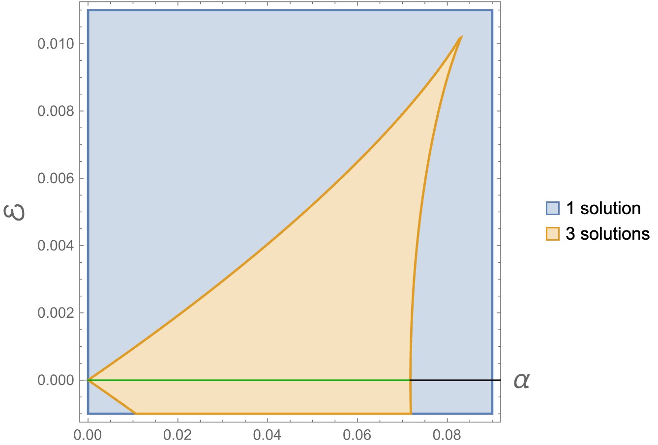
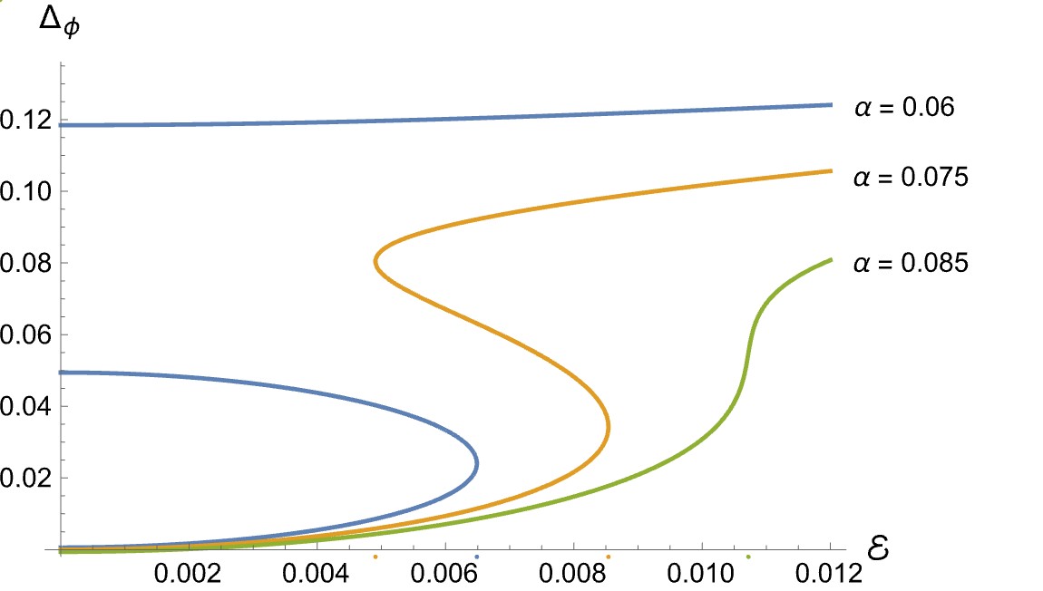
Figure 1: Left: Plot of the number of acceptable solutions to (3.29) for $p=q=3$ as a function of $\alpha$ and $\mathcal{E}$. For $\mathcal{E}>0$ there are 3 solutions in the yellow region, 1 solution in the blue region, and 2 solutions along their boundary. For $\mathcal{E}=0$ there are two solutions along the green segment, no solutions along the black line, and 1 solution at their boundary. Right: Solutions $\Delta_{\phi}(\mathcal{E})$ for $\alpha=0.06$, $0.075$, $0.085$.

There are special values of $\mathcal{E}$ and $\alpha$ for which (3.38) simplifies. For $\alpha=1$, (3.38) reduces to a quadratic equation and the unique solution with $\Delta_{\phi}\in\bigl{(}0,\frac{1}{2p}\bigr{)}$ is

$$\Delta_{\phi}=\frac{1}{4p}-\frac{1}{2\pi}\arcsin\biggl{[}\frac{\sin\bigl{(}\frac{\pi}{2p}\bigr{)}}{\cosh(2\pi p\mathcal{E})}\biggr{]}\;,$$ (3.39)

acceptable whenever $\mathcal{E}>0$. The corresponding solution to (3.30) is

$$g_{\eta}^{p}\,g_{\phi}^{p}=\frac{p\sin\bigl{(}\frac{\pi}{2p}\bigr{)}}{2\pi J\sqrt{\cosh^{2}(2\pi p\mathcal{E})-\sin^{2}\bigl{(}\frac{\pi}{2p}\bigr{)}}}\;.$$ (3.40)

For $\mathcal{E}=0$, (3.38) can be written as a quadratic equation in $\tan(\pi\Delta_{\phi})$ which gives two solutions:

$$\Delta_{\phi}=\frac{1}{\pi}\arctan\biggl{[}\frac{1-\alpha}{2}\,\tan\Bigl{(}\frac{\pi}{2p}\Bigr{)}\pm\frac{1}{2}\sqrt{(1-\alpha)^{2}\tan^{2}\Bigl{(}\frac{\pi}{2p}\Bigr{)}-4\alpha}\,\biggr{]}\;.$$ (3.41)

The two solutions are real if and only if $\alpha\leq\tan^{2}\bigl{(}\frac{\pi}{4p}\bigr{)}$. Indeed $\alpha=\tan^{2}\big{(}\frac{\pi}{4p}\bigr{)}$ is where the right boundary of the yellow region intersects the horizontal axis in Figure 1 and the two solutions merge into one (disappearing for larger values of $\alpha$). It follows from (3.41) that both solutions satisfy $\Delta_{\phi}>0$, that the larger solution becomes $\Delta_{\phi}=\frac{1}{2p}$ for $\alpha=0$, and that $\Delta_{\phi}<\frac{1}{2p}$ for the allowed values $\alpha>0$. The corresponding solution to (3.30) is

$$g_{\eta}^{p}\,g_{\phi}^{p}=\frac{\alpha\,p}{2\pi J\tan(\pi\Delta_{\phi})}\;.$$ (3.42)

Case $\boldsymbol{p>1}$, $\boldsymbol{q=1}$.

The behaviour of the function $R_{p,1,\mathcal{E}}(\Delta_{\phi})$ is similar to the one in the previous case, however the function $\sin(2\pi\Delta_{\phi})$ vanishes at both endpoints $\Delta_{\phi}=0,\frac{1}{2}$. For very small values of $\alpha$, the number of solutions $\Delta_{\phi}(\mathcal{E})$ to (3.29) as we increase $\mathcal{E}$ from above $0$ to $+\infty$ is 2 (of which only 1 is acceptable at $\mathcal{E}=0$) and then 0. For larger values of $\alpha$ it is 1 (not acceptable at $\mathcal{E}=0$), then 2, and then 0. For even larger values of $\alpha$ there is only 1 solution (that becomes $\Delta_{\phi}=0$ at $\mathcal{E}=0$ and thus is not acceptable) up to $\mathcal{E}_{*}(\alpha)$ and then no solutions for $\mathcal{E}\geq\mathcal{E}_{*}(\alpha)$.

3.5 Solutions at large $\boldsymbol{p}$ and fixed $\boldsymbol{q}$

Using the methods in [6, 11] and Appendix C of [12], we search for analytic solutions to the Schwinger–Dyson equations at large $p$. We truncate to the bosonic components only, assuming (3.12), but we do not neglect the kinetic terms. Let the chemical potentials corresponding to $Q_{\eta,\phi}$ be $\mu_{\eta,\phi}$ respectively. The equations we want to solve are the algebraic ones in (3.13) and the integro-differential ones in (3.8) that in components read as in (B.5):

$$-\bigl{(}\partial_{\tau_{2}}+\mu_{\eta}\bigr{)}\,G_{\overline{\eta}\eta}(\tau_{1},\tau_{2})+\int\!d\tau_{3}\,\Sigma_{\overline{\eta}\eta}(\tau_{2},\tau_{3})\,G_{\overline{\eta}\eta}(\tau_{1},\tau_{3}) =\delta(\tau_{1}-\tau_{2})\;,$$ (3.43)

$$G_{\overline{f}f}(\tau_{1},\tau_{2})+\int\!d\tau_{3}\,\Sigma_{\overline{f}f}(\tau_{2},\tau_{3})\,G_{\overline{f}f}(\tau_{1},\tau_{3}) =-\delta(\tau_{1}-\tau_{2})\;,$$

$$-\bigl{(}\partial_{\tau_{2}}+\mu_{\phi}\bigr{)}\,G_{\overline{\phi}\phi}(\tau_{1},\tau_{2})+\int\!d\tau_{3}\,\Sigma_{\overline{\phi}\phi}(\tau_{2},\tau_{3})\,G_{\overline{\phi}\phi}(\tau_{1},\tau_{3}) =-\alpha\,\delta(\tau_{1}-\tau_{2})\;,$$

$$G_{\overline{\psi}\psi}(\tau_{1},\tau_{2})+\int\!d\tau_{3}\,\Sigma_{\overline{\psi}\psi}(\tau_{2},\tau_{3})\,G_{\overline{\psi}\psi}(\tau_{1},\tau_{3}) =\alpha\,\delta(\tau_{1}-\tau_{2})\;.$$

Assuming that the theory becomes free in the large $p$ limit, we search for solutions in a $\frac{1}{p}$ expansion around the free two-point functions. Generically, we expand the bilocal fields $G$ (assuming translational invariance) as

$$G(\tau) =G_{0}(\tau)+\frac{1}{p^{n}}G_{1}(\tau)+\mathcal{O}(p^{-n-1})\;,$$ (3.44)

$$G(\omega_{k}) =G_{0}(\omega_{k})+\frac{1}{p^{n}}G_{1}(\omega_{k})+\mathcal{O}(p^{-n-1})\;.$$

Here $G_{0}$ are the free propagators (we review the correlators of free Fermi and chiral multiplets in Appendix C), $\omega_{k}$ are the appropriate Matsubara frequencies, $n>0$ are suitable integers that we determine below, and we require

$$\bigl{\lvert}G_{0}(\omega_{k})\bigr{\rvert}\,\gg\,\frac{\lvert G_{1}(\omega_{k})\rvert}{p^{n}}\;,\qquad\forall\,\omega_{k}\text{ fixed}\,,\quad p\gg 1\;.$$ (3.45)

More in detail, substituting the free propagators (C.16), (C.20), (C.24), (C.28) into the definition (B.2) of the bilocal fields, one obtains:

$$G_{\bar{\eta}\eta}^{(0)}(\tau) =\hskip 6.99997pt\frac{e^{\mu_{\eta}\tau}}{2\cosh\bigl{(}\frac{\mu_{\eta}\beta}{2}\bigr{)}}\Bigl{[}\Theta(\tau)\,e^{-\frac{\mu_{\eta}\beta}{2}}-\Theta(-\tau)\,e^{\frac{\mu_{\eta}\beta}{2}}\Bigr{]}\;,\quad G_{\bar{f}f}^{(0)}(\tau) =-\delta(\tau)\;,$$ (3.46)

$$G_{\bar{\phi}\phi}^{(0)}(\tau) =\alpha\,\frac{e^{\mu_{\phi}\tau}}{2\sinh\bigl{(}\frac{\mu_{\phi}\beta}{2}\bigr{)}}\Bigl{[}\Theta(\tau)\,e^{-\frac{\mu_{\phi}\beta}{2}}+\Theta(-\tau)\,e^{\frac{\mu_{\phi}\beta}{2}}\Bigr{]}\;,\quad G_{\bar{\psi}\psi}^{(0)}(\tau) =\alpha\,\delta(\tau)\;.$$

Being them free propagators, they satisfy the free equations of motion, obtained from (3.43) by setting all $\Sigma$’s to zero. We consider an ansatz for the bilocal fields that is an expansion in $\frac{1}{p}$ around the free result:

$$G_{\bar{\eta}\eta}(\tau) =G_{\bar{\eta}\eta}^{(0)}(\tau)\biggl{(}1+\frac{\widetilde{G}_{\bar{\eta}\eta}(\tau)}{p}+\mathcal{O}(p^{-2})\biggr{)}, G_{\bar{f}f}(\tau) =-\delta(\tau)+\frac{\widetilde{G}_{\bar{f}f}(\tau)}{p^{n_{f}}}+\mathcal{O}\bigl{(}p^{-n_{f}-1}\bigr{)},$$

$$G_{\bar{\phi}\phi}(\tau) =G_{\bar{\phi}\phi}^{(0)}(\tau)\biggl{(}1+\frac{\widetilde{G}_{\bar{\phi}\phi}(\tau)}{p^{n_{\phi}}}+\mathcal{O}\bigl{(}p^{-n_{\phi}-1}\bigr{)}\biggr{)}, G_{\bar{\psi}\psi}(\tau) =\alpha\,\delta(\tau)+\frac{\widetilde{G}_{\bar{\psi}\psi}(\tau)}{p^{n_{\psi}}}+\mathcal{O}\bigl{(}p^{-n_{\psi}-1}\bigr{)}.$$ (3.47)

Here we assume that $n_{f},n_{\phi},n_{\psi}>0$ and that $\widetilde{G}_{\bar{\eta}\eta}$, $\widetilde{G}_{\bar{f}f}$, $\widetilde{G}_{\bar{\phi}\phi}$, $\widetilde{G}_{\bar{\psi}\psi}$ are $\mathcal{O}(1)$. We chose the order of the leading correction in $G_{\bar{\eta}\eta}$ such that various terms in the equations of motion simplify using

$$\bigl{[}G_{\bar{\eta}\eta}\bigr{]}^{p-n}=\bigl{[}G_{\bar{\eta}\eta}^{(0)}\bigr{]}^{p-n}\,e^{\widetilde{G}_{\bar{\eta}\eta}}\,\bigl{(}1+\mathcal{O}(p^{-1})\bigr{)}\;.$$ (3.48)

This in turn leads to the same differential equation as in [6, 11], with the benefit of hindsight. In terms of the chemical potentials $\mu_{F}$ for $\mathrm{U}(1)_{F}$ and $\mu_{R}$ for any R-charge $\mathrm{U}(1)_{R}$, the potentials $\mu_{\eta,\phi}$ are decomposed as

$$\mu_{\eta}=q\,\mu_{F}+R[\eta]\,\mu_{R}\;,\qquad\mu_{\phi}=-p\,\mu_{F}+R[\phi]\,\mu_{R}\;,\qquad p\,\mu_{\eta}+q\,\mu_{\phi}=\mu_{R}\;.$$ (3.49)

The last equation follows from the constraint that the J-term has R-charge $1$, i.e., from $p\,R[\eta]+q\,R[\phi]=1$ . We want to be able to impose the supersymmetry constraint $\mu_{R}=0$ at large $p$. This implies that the scalings of $\mu_{\eta}$ and $\mu_{\phi}$ must be related as $\mu_{\phi}\sim p\,\mu_{\eta}$. The simplest scaling is $\mu_{\eta}\sim\mu_{F}\sim R[\eta]\sim\mathcal{O}(p^{-1})$ and $\mu_{\phi}\sim\mu_{R}\sim R[\phi]\sim\mathcal{O}(1)$. In this way both $G_{\bar{\eta}\eta}^{(0)}$ and $G_{\bar{\phi}\phi}^{(0)}$ are $\mathcal{O}(1)$. Besides, the bilocal fields should agree with the free limits at short distances, which implies the following boundary conditions: $\widetilde{G}(0)=\widetilde{G}(\beta)=0$ for all components. Plugging the ansatz (3.47) and the boundary conditions into (3.43) we get

$$0 =\frac{1}{p}\,G_{\bar{\eta}\eta}^{(0)}(\tau_{12})\,\partial_{\tau_{12}}\widetilde{G}_{\bar{\eta}\eta}(\tau_{12})+\int\!d\tau_{3}\,\Sigma_{\bar{\eta}\eta}(\tau_{23})\,G_{\bar{\eta}\eta}^{(0)}(\tau_{13})+\mathcal{O}(p^{-2})\;,$$ (3.50)

$$0 =\frac{1}{p^{n_{f}}}\widetilde{G}_{\bar{f}f}(\tau_{12})-\Sigma_{\bar{f}f}(\tau_{21})+\mathcal{O}\bigl{(}p^{-n_{f}-1}\bigr{)}\;,$$

$$0 =\frac{1}{p^{n_{\phi}}}\,G_{\bar{\phi}\phi}^{(0)}(\tau_{12})\,\partial_{\tau_{12}}\widetilde{G}_{\bar{\phi}\phi}(\tau_{12})+\int\!d\tau_{3}\,\Sigma_{\bar{\phi}\phi}(\tau_{23})\,G_{\bar{\phi}\phi}^{(0)}(\tau_{13})+\mathcal{O}\bigl{(}p^{-n_{\phi}-1}\bigr{)}\;,$$

$$0 =\frac{1}{p^{n_{\psi}}}\widetilde{G}_{\bar{\psi}\psi}(\tau_{12})+\alpha\,\Sigma_{\bar{\psi}\psi}(\tau_{21})+\mathcal{O}\bigl{(}p^{-n_{\psi}-1}\bigr{)}\;,$$

where $\tau_{ij}=\tau_{i}-\tau_{j}$. These equations can be solved to obtain the $\Sigma$’s in terms of the $G$’s at leading order in $\frac{1}{p}$. In particular, one acts with $(\partial_{\tau_{1}}-\mu_{\eta})$ on the first equation and with $(\partial_{\tau_{1}}-\mu_{\phi})$ on the third equation, obtaining:

$$\Sigma_{\bar{\eta}\eta}(-\tau) =-\tfrac{1}{p}\,G_{\bar{\eta}\eta}^{(0)}(\tau)\,\partial_{\tau}^{2}\widetilde{G}_{\bar{\eta}\eta}(\tau)+\mathcal{O}(p^{-2}),\hskip 21.00009pt\Sigma_{\bar{f}f}(-\tau)=\tfrac{1}{p^{n_{f}}\rule{0.0pt}{4.68999pt}}\,\widetilde{G}_{\bar{f}f}(\tau)+\mathcal{O}(p^{-n_{f}-1}),$$ (3.51)

$$\Sigma_{\bar{\phi}\phi}(-\tau) =\tfrac{1}{\alpha p^{n_{\phi}}\rule{0.0pt}{4.68999pt}}\,G_{\bar{\phi}\phi}^{(0)}(\tau)\,\partial_{\tau}^{2}\widetilde{G}_{\bar{\phi}\phi}(\tau)+\mathcal{O}(p^{-n_{\phi}-1}),\;\;\Sigma_{\bar{\psi}\psi}(-\tau)=-\tfrac{1}{\alpha p^{n_{\psi}}\rule{0.0pt}{4.68999pt}}\,\widetilde{G}_{\bar{\psi}\psi}(\tau)+\mathcal{O}(p^{-n_{\psi}-1}).$$

Let us then consider the algebraic equations. Substituting the ansatz (3.47) into the last two equations of (3.13) we determine the leading behavior of $\Sigma_{\bar{f}f}$ and $\Sigma_{\bar{\psi}\psi}$. This can then be used in (3.51) to determine $\widetilde{G}_{\bar{f}f}$ and $\widetilde{G}_{\bar{\psi}\psi}$. In order to have a well-defined large $p$ limit, the simplest choice is to scale $J$ as $2^{p}p^{-n_{f}}$, so that the combination

$$\mathcal{J}\,\equiv\,\frac{\alpha^{q}\,p^{n_{f}}\,J}{2^{p+q-2}\,q\cosh^{p-2}\bigl{(}\frac{\mu_{\eta}\beta}{2}\bigr{)}\sinh^{q}\bigl{(}\frac{\mu_{\phi}\beta}{2}\bigr{)}}$$ (3.52)

remains fixed as $p$ becomes large. Recalling that $p$ is odd, we obtain:

$$\widetilde{G}_{\bar{f}f}(\tau) =\frac{\mathcal{J}\,e^{\left(\mu_{\eta}-\mu_{R}\right)\tau}}{2\cosh\bigl{(}\frac{\mu_{\eta}\beta}{2}\bigr{)}}\,\Bigl{[}\Theta(\tau)\>e^{-\left(\mu_{\eta}-\mu_{R}\right)\frac{\beta}{2}}+\Theta(-\tau)\>e^{\left(\mu_{\eta}-\mu_{R}\right)\frac{\beta}{2}}\Bigr{]}\,e^{\widetilde{G}_{\bar{\eta}\eta}(-\tau)}\;,$$ (3.53)

$$\widetilde{G}_{\bar{\psi}\psi}(\tau) =\frac{q\,\mathcal{J}\,\sinh\bigl{(}\tfrac{\mu_{\phi}\beta}{2}\bigr{)}\,e^{(\mu_{\phi}-\mu_{R})\tau}}{2\cosh^{2}\bigl{(}\frac{\mu_{\eta}\beta}{2}\bigr{)}}\,\Bigl{[}\Theta(\tau)\>e^{-(\mu_{\phi}-\mu_{R})\frac{\beta}{2}}-\Theta(-\tau)\>e^{(\mu_{\phi}-\mu_{R})\frac{\beta}{2}}\Bigr{]}\,e^{\widetilde{G}_{\bar{\eta}\eta}(-\tau)}\;,$$

together with $n_{\psi}=n_{f}+1$. Similarly, substituting these expressions and the ansatz (3.47) into the first two equations of (3.13), we determine the leading behavior of $\Sigma_{\bar{\eta}\eta}$ and $\Sigma_{\bar{\phi}\phi}$:

$$\Sigma_{\bar{\eta}\eta}(\tau) =-\frac{\mathcal{J}^{2}}{p^{2n_{f}-1}}\;G^{(0)}_{\bar{\eta}\eta}(-\tau)\;e^{\widetilde{G}_{\bar{\eta}\eta}(\tau)+\widetilde{G}_{\bar{\eta}\eta}(-\tau)}+\mathcal{O}(p^{-2n_{f}})\;,$$ (3.54)

$$\Sigma_{\bar{\phi}\phi}(\tau) =\frac{q\,\mathcal{J}^{2}\,\sinh^{2}\bigl{(}\frac{\mu_{\phi}\beta}{2}\bigr{)}}{p^{2n_{f}}\,\alpha^{2}\,\cosh^{2}\bigl{(}\frac{\mu_{\eta}\beta}{2}\bigr{)}}\;G_{\bar{\phi}\phi}^{(0)}(-\tau)\;e^{\widetilde{G}_{\bar{\eta}\eta}(\tau)+\widetilde{G}_{\bar{\eta}\eta}(-\tau)}+\mathcal{O}(p^{-2n_{f}-1})\;.$$

Equating these expressions with those in (3.51) to leading order in $\tfrac{1}{p}$ fixes $n_{f}=1$ and $n_{\phi}=n_{\psi}=2$, and gives the following differential equations:

$$\partial_{\tau}^{2}\,\widetilde{G}_{\bar{\eta}\eta}(\tau)=\mathcal{J}^{2}\;e^{\widetilde{G}_{\bar{\eta}\eta}(\tau)+\widetilde{G}_{\bar{\eta}\eta}(-\tau)}\,,\qquad\partial_{\tau}^{2}\,\widetilde{G}_{\bar{\phi}\phi}(\tau)=\frac{q\,\mathcal{J}^{2}\,\sinh^{2}\bigl{(}\tfrac{\mu_{\phi}\beta}{2}\bigr{)}}{\alpha\,\cosh^{2}\bigl{(}\frac{\mu_{\eta}\beta}{2}\bigr{)}}\;e^{\widetilde{G}_{\bar{\eta}\eta}(\tau)+\widetilde{G}_{\bar{\eta}\eta}(-\tau)}\,.$$ (3.55)

Notice that the free propagators $G_{\bar{\eta}\eta}^{(0)}$ and $G_{\bar{\phi}\phi}^{(0)}$ have dropped from the equations. The only solution to the second equation that satisfies the boundary conditions is

$$\widetilde{G}_{\bar{\phi}\phi}(\tau)=\frac{q\,\sinh^{2}\bigl{(}\tfrac{\mu_{\phi}\beta}{2}\bigr{)}}{\alpha\,\cosh^{2}\bigl{(}\frac{\mu_{\eta}\beta}{2}\bigr{)}}\;\widetilde{G}_{\bar{\eta}\eta}\;.$$ (3.56)

The differential equation for $\widetilde{G}_{\bar{\eta}\eta}$ is the same as the one found in [6, 12, 11]. Since the odd part $\widetilde{G}_{\text{odd}}(\tau)=\frac{1}{2}\bigl{(}\widetilde{G}_{\bar{\eta}\eta}(\tau)-\widetilde{G}_{\bar{\eta}\eta}(-\tau)\bigr{)}$ satisfies $\partial_{\tau}^{2}\,\widetilde{G}_{\text{odd}}(\tau)=0$, the only solution compatible with the boundary conditions is $\widetilde{G}_{\text{odd}}(\tau)=0$ and we can take $\widetilde{G}_{\bar{\eta}\eta}$ to be even. Then the general solution with integration constants $v,b$ is: $\exp\bigl{[}\widetilde{G}_{\bar{\eta}\eta}(\tau)\bigr{]}=v/\bigl{[}\beta\mathcal{J}\sin\bigl{(}\frac{v}{\beta}|\tau|+b\bigr{)}\bigr{]}$ where $v>0$, $\beta$ has been introduced for later convenience, and $b$ is defined modulo $2\pi$. The boundary conditions $\widetilde{G}(0)=\widetilde{G}(\beta)=0$ imply $\beta\mathcal{J}=v/\sin(b)$ and $\sin(b)=\sin(v+b)$. One solution to the second equation is $v=2\pi m$ for $m\in\mathbb{N}$, however this does not lead to a function $\exp\bigl{[}\widetilde{G}_{\bar{\eta}\eta}(\tau)\bigr{]}$ that is positive for all values of $\tau$. The other solutions are $b=\bigl{(}n+\frac{1}{2}\bigr{)}\pi-\frac{v}{2}$ for $n\in\mathbb{Z}$ and without loss of generality we consider $n=0,1$. The other equation reduces to $\beta\mathcal{J}=\pm v/\cos\bigl{(}\frac{v}{2}\bigr{)}$, where $\pm$ correspond to $n=0,1$, respectively. Only the case $n=0$, $0<v<\pi$ leads to a positive function $\exp\bigl{[}\widetilde{G}_{\bar{\eta}\eta}(\tau)\bigr{]}$, and the second equation has one and only one solution for all values of $\beta$. The final solution is thus:

$$e^{\widetilde{G}_{\bar{\eta}\eta}(\tau)}=\frac{v}{\beta\mathcal{J}\cos\bigl{(}\frac{v}{\beta}|\tau|-\frac{v}{2}\bigr{)}}\;,\qquad\beta\mathcal{J}=\frac{v}{\cos\bigl{(}\frac{v}{2}\bigr{)}}\;,\qquad 0<v<\pi\;.$$ (3.57)

In the weak coupling limit $\beta\mathcal{J}\rightarrow 0$ (keeping all $\mu_{I}\beta$’s fixed) one has $v\to 0$ and $\frac{v}{\beta\mathcal{J}}\rightarrow 1$ and therefore $\widetilde{G}_{\bar{\eta}\eta},\,\widetilde{G}_{\bar{\phi}\phi}\to 0$. From (3.53) we see that also $\widetilde{G}_{\bar{f}f},\,\widetilde{G}_{\bar{\psi}\psi}\to 0$ and the solution reduces to the free UV one at leading order in $\tfrac{1}{p}$. In the strong coupling limit $\beta\mathcal{J}\rightarrow\infty$, instead, one has $v\rightarrow\pi$ and, to this order of approximation and away from $\tau=0$, the two-point functions agree with the conformal ones (3.17) with the following parameters:

$$\Delta_{\eta} =\frac{1}{2p}+\mathcal{O}(p^{-2})\;, 2\pi\mathcal{E}_{\eta} =-\beta\mu_{\eta}+\mathcal{O}(p^{-2})\;,$$

$$\Delta_{f} =\frac{1}{2}+\mathcal{O}(p^{-1})\;, 2\pi\mathcal{E}_{f} =\beta(\mu_{R}-\mu_{\eta})+\mathcal{O}(p^{-1})\;,$$ (3.58)

$$\Delta_{\phi} =\frac{q\,\sinh^{2}\bigl{(}\tfrac{\mu_{\phi}\beta}{2}\bigr{)}}{2\alpha p^{2}\,\cosh^{2}\bigl{(}\frac{\mu_{\eta}\beta}{2}\bigr{)}}+\mathcal{O}(p^{-3})\;,\quad 2\pi\mathcal{E}_{\phi} =-\beta\mu_{\phi}+\mathcal{O}(p^{-3})\;,$$

$$\Delta_{\psi} =\frac{1}{2}+\mathcal{O}(p^{-1})\;, 2\pi\mathcal{E}_{\psi} =\beta(\mu_{R}-\mu_{\phi})+\mathcal{O}(p^{-1})\;,$$

as well as

$$g_{\eta} =\frac{1}{2\cosh\bigl{(}\frac{\mu_{\eta}\beta}{2}\bigr{)}}\biggl{(}1-\frac{1}{p}\log\mathcal{J}\biggr{)}+\mathcal{O}(p^{-2})\,,\hskip 45.00006ptg_{f}=\frac{1}{2p\cosh\bigl{(}\frac{\mu_{\eta}\beta}{2}\bigr{)}}+\mathcal{O}(p^{-2})\,,$$ (3.59)

$$g_{\phi} =\frac{\alpha}{2\sinh\bigl{(}\frac{\mu_{\phi}\beta}{2}\bigr{)}}\biggl{(}1-\frac{q\sinh^{2}\bigl{(}\tfrac{\mu_{\phi}\beta}{2}\bigr{)}}{\alpha p^{2}\cosh^{2}\bigl{(}\frac{\mu_{\eta}\beta}{2}\bigr{)}}\log\mathcal{J}\biggr{)}+\mathcal{O}(p^{-3})\,,\quad g_{\psi}=\frac{q\sinh\bigl{(}\tfrac{\mu_{\phi}\beta}{2}\bigr{)}}{2p^{2}\cosh^{2}\bigl{(}\frac{\mu_{\eta}\beta}{2}\bigr{)}}+\mathcal{O}(p^{-3}).$$

The conformal dimensions are compatible with the bounds (3.24) at leading order in $\tfrac{1}{p}$, in particular $\Delta_{\eta}$ saturates $p\Delta_{\eta}=\frac{1}{2}+\mathcal{O}(p^{-1})$. A higher order in $\tfrac{1}{p}$ it would be necessary to verify that all bounds are satisfied. We see that the condition $\mu_{\phi}>0$ (discussed in Section 2) is necessary in order to ensure $g_{\phi},g_{\psi}>0$ as required by unitarity. We tentatively see that the solution at large $p$ interpolates between the free UV limit and the IR conformal-like behavior. Notice in particular that the phase transition is not visible in this limit.

It might be tempting to think that the conformal data in (3.58) solves, at some given order in $\frac{1}{p}$, the self-consistency equations (3.23). This, in general, does not happen, due to incompatibility between the large $p$ and low energy limits. Write (3.43) in Fourier space:

$$\biggl{[}-\frac{s}{G_{0}(\omega_{k})}+\beta^{2}\,\Sigma(\omega_{-k})\biggr{]}G(\omega_{k})=-s\;,$$ (3.60)

where $\Sigma$ should again be understood as $\alpha^{-1}\Sigma$ for $\phi$ and $\psi$, and we used that $G_{0}$ is the free propagator. In the large $p$ limit (3.45), using the expansion (3.44), one further has

$$\Sigma(\omega_{-k})=\frac{-s}{\beta^{2}G_{0}(\omega_{k})+\frac{\beta^{2}}{p^{n}}G_{1}(\omega_{k})+\mathcal{O}\bigl{(}\frac{1}{p^{n+1}}\bigr{)}}+\frac{s}{\beta^{2}G_{0}(\omega_{k})}=\frac{s}{p^{n}}\frac{G_{1}(\omega_{k})}{\beta^{2}G_{0}(\omega_{k})^{2}}+\mathcal{O}\bigl{(}\tfrac{1}{p^{n+1}}\bigr{)}.$$ (3.61)

In these terms, as one can see from (3.43), the low-energy regime we previously studied for dynamical and auxiliary fields, respectively, corresponds to taking

$$\bigl{\lvert}\mu_{\phi,\eta}-\beta\,\Sigma_{\phi,\eta}(\omega_{-k})\bigr{\rvert}\gg|\omega_{k}|\;,\qquad\bigl{\lvert}\beta\,\Sigma_{f,\psi}(\omega_{-k})\bigr{\rvert}\gg 1\;,\qquad\omega_{k}\ll J\;.$$ (3.62)

Combining with (3.61), for the auxiliary fields we find that

$$\frac{1}{p^{n}}\,\bigl{\lvert}G_{1}(\omega_{k})\bigr{\rvert}\gg\bigl{\lvert}G_{0}(\omega_{k})\bigr{\rvert}\;,$$ (3.63)

which directly contradicts (3.45) (recall that $\bigl{\lvert}G_{0}(\omega_{k})\bigr{\rvert}=1/\beta$ for auxiliary fields). This means that, as long as we must include auxiliary fields in our considerations, there is no regime of large $p$ and small $\omega_{k}$ in which the approximation we made in our large $p$ computation and the approximation of dropping the kinetic terms are both reliable.

This result suggests that, at large $p$, the system at low energies first enters into a quasi-conformal regime described by (3.58)–(3.59) in which interactions compete with the kinetic terms, while at extremely low temperatures the system ends up in a different conformal regime that satisfies (3.22)–(3.23) and in which the kinetic terms are negligible.

A particular case, in this respect, is the supersymmetric one for which $\mu_{R}=0$. In this case the IR conformal solution is supersymmetric since its parameters satisfy the constraints (3.26)–(3.27) within the working accuracy. Moreover, (3.29) can be independently derived from $\mathcal{I}$-extremization, as we will do in Section 3.9, without assuming (3.63). At this point, the zero-temperature limit where the index is computed can be taken safely by requiring that $p$ goes to infinity faster than $G_{1}(\omega)$ as $\omega$ goes to zero, in such a way that (3.45) holds. Because of this, (3.58)–(3.59) in the supersymmetric regime do actually solve (3.29).

3.5.1 Grand potential and entropy at large $\boldsymbol{p}$

It is possible to compute the grand potential $\log Z$ in a large $p$ expansion. To leading order in $1/N$, this is just the averaged action (3.6) (or (B.3) in components) evaluated on the solution provided by (3.57). Instead of a direct evaluation, we follow [11, 12] and first compute the derivative of $\log Z$ with respect to $J$. Only the explicit dependence on $J$ in (3.6) matters when taking this derivative, and not the dependence through dimensionful coefficients such as $g_{\eta,\phi}$ in the bilocal fields $G_{\eta,\phi}$ since the fields solve the equations of motion. We get:

$$J\,\partial_{J}\,\frac{\log Z}{N}=J\int\!d\tau_{1}\,d\tau_{2}\,\biggl{(}\frac{1}{q}\,G_{\bar{f}f}\,G_{\bar{\eta}\eta}^{p-1}\,G_{\bar{\phi}\phi}^{q}+\frac{1}{p}\,G_{\bar{\eta}\eta}^{p}\,G_{\bar{\psi}\psi}\,G_{\bar{\phi}\phi}^{q-1}\biggr{)}$$ (3.64)

$$\,\,\qquad\qquad=\frac{\mathcal{J}^{2}\cos^{2}\bigl{(}\frac{v}{2}\bigr{)}}{4p^{2}\cosh^{2}\bigl{(}\frac{\mu_{\eta}\beta}{2}\bigr{)}}\int_{-\beta}^{\beta}\!d\tau\,\frac{\beta-|\tau|}{\cos^{2}\bigl{(}\frac{v}{\beta}|\tau|-\frac{v}{2}\bigr{)}}+\mathcal{O}(p^{-3})=\frac{v\tan\bigl{(}\frac{v}{2}\bigr{)}}{2p^{2}\cosh^{2}\bigl{(}\frac{\mu_{\eta}\beta}{2}\bigr{)}}+\mathcal{O}(p^{-3})\,.$$

To the integral on the first line the delta functions in $G_{\bar{f}f}$ and $G_{\bar{\psi}\psi}$ do not contribute, and hence only the first term contributes at leading order, since the second term is suppressed by $\tfrac{1}{p^{2}}$ with respect to the first one. Using the relation between $\beta\mathcal{J}$ and $v$ in (3.57) as well as the linearity of $\beta\mathcal{J}$ in $J$ in (3.52), the derivative with respect to $J$ can be exchanged for a derivative with respect to $v$ using the formula $J\,\partial_{J}=v/\bigl{[}1+\frac{v}{2}\tan\bigl{(}\frac{v}{2}\bigr{)}\bigr{]}\,\partial_{v}$. We obtain a differential equation in $v$ for $\log Z$:

$$\frac{1}{N}\,\partial_{v}\log Z=\frac{\tan\bigl{(}\frac{v}{2}\bigr{)}\,\bigl{[}1+\frac{v}{2}\tan\bigl{(}\frac{v}{2}\bigr{)}\bigr{]}}{2p^{2}\cosh^{2}\bigl{(}\frac{\mu_{\eta}\beta}{2}\bigr{)}}+\mathcal{O}(p^{-3})\;.$$ (3.65)

The value of $\log Z$ at $v=0$ is known because at that point the theory is free. We can read off $Z\big{|}_{v=0}$ from (C.18) and (C.26). Integrating (3.65) from $0$ to $v$ at large $p$ then gives

$$\frac{\log Z}{N}=\log\biggl{[}2\cosh\biggl{(}\frac{\mu_{\eta}\beta}{2}\biggr{)}\biggr{]}-\alpha\log\biggl{[}2\sinh\biggl{(}\frac{\mu_{\phi}\beta}{2}\biggr{)}\biggr{]}+\frac{v\tan\bigl{(}\frac{v}{2}\bigr{)}-\frac{v^{2}}{4}}{2p^{2}\cosh^{2}\bigl{(}\frac{\mu_{\eta}\beta}{2}\bigr{)}}+\mathcal{O}(p^{-3})\;.$$ (3.66)

As $p\rightarrow\infty$, $\log Z$ tends to the free value, which is consistent with our starting ansatz (3.47).

In order to compute the von Neumann entropy $S=(1-\beta\partial_{\beta})\log Z$, one needs to make the $\beta$ dependence in $v$ explicit. Using $\beta\partial_{\beta}=\beta\mathcal{J}\cos\bigl{(}\frac{v}{2}\bigr{)}/\bigl{[}1+\frac{v}{2}\tan\bigl{(}\frac{v}{2}\bigr{)}\bigr{]}\cdot\partial_{v}$ we obtain

$$\frac{S}{N} =\log\biggl{[}2\cosh\biggl{(}\frac{\mu_{\eta}\beta}{2}\biggr{)}\biggr{]}-\frac{\mu_{\eta}\beta}{2}\tanh\biggl{(}\frac{\mu_{\eta}\beta}{2}\biggr{)}-\alpha\log\biggl{[}2\sinh\biggl{(}\frac{\mu_{\phi}\beta}{2}\biggr{)}\biggr{]}+\frac{\alpha\mu_{\phi}\beta}{2}\coth\biggl{(}\frac{\mu_{\phi}\beta}{2}\biggr{)}$$

$$\quad-\frac{v^{2}}{8p^{2}\cosh^{2}\bigl{(}\frac{\mu_{\eta}\beta}{2}\bigr{)}}+\mathcal{O}(p^{-3})\;.$$ (3.67)

On the first line is the entropy of the free theory, as in (C.19) and (C.27), while on the second line is the first correction. In order to obtain the low-temperature behavior, we take $\beta\mathcal{J}\rightarrow\infty$ while keeping $\beta\mu_{\eta,\phi}$ fixed and expand $v(\beta\mathcal{J})$ in (3.57):

$$v^{2}=\pi^{2}-\frac{4\pi^{2}}{\beta\mathcal{J}}+\frac{12\pi^{2}}{(\beta\mathcal{J})^{2}}+\mathcal{O}\bigl{(}(\beta\mathcal{J})^{-3}\bigr{)}\;.$$ (3.68)

In particular, the zero-temperature specific entropy $\mathcal{S}_{0}\,\equiv\,S\bigl{(}\beta=\infty\bigr{)}/N$ can be expressed using the relations $\beta\mu_{\eta,\phi}=-2\pi\mathcal{E}_{\eta,\phi}$ between the chemical potentials and the spectral asymmetries of the IR conformal solution, which are valid at zero temperature:

$$\mathcal{S}_{0} =\log\bigl{[}2\cosh(-\pi\mathcal{E}_{\eta})\bigr{]}-\pi\mathcal{E}_{\eta}\tanh(\pi\mathcal{E}_{\eta})-\alpha\log\bigl{[}2\sinh(-\pi\mathcal{E}_{\phi})\bigr{]}+\alpha\,\pi\mathcal{E}_{\phi}\coth(\pi\mathcal{E}_{\phi})$$

$$\quad-\frac{\pi^{2}}{8p^{2}\cosh^{2}\bigl{(}\frac{\mu_{\eta}\beta}{2}\bigr{)}}+\mathcal{O}(p^{-3})\;.$$ (3.69)

We shall see in Section 3.9 that this quantity, when evaluated on supersymmetric spectral asymmetries satisfying $p\mathcal{E}_{\eta}+q\mathcal{E}_{\phi}=0$, matches the large $p$ expansion of the entropy extracted from the Witten index.

3.6 Solutions at large $\boldsymbol{p}$ and $\boldsymbol{q}$

We can similarly search for analytic solutions to the Schwinger-Dyson equations at large $p$ and $q$, following the same steps as in Section 3.5. We consider an ansatz for the bilocal fields similar to the one in (3.47), however we keep the ratio $p/q$ fixed as we send $p\to\infty$:

$$G_{\bar{\eta}\eta}(\tau) =G_{\bar{\eta}\eta}^{(0)}(\tau)\biggl{(}1+\frac{1}{p}\widetilde{G}_{\bar{\eta}\eta}(\tau)+\mathcal{O}(p^{-2})\biggr{)}\,,\;\; G_{\bar{f}f}(\tau) =-\delta(\tau)+\frac{1}{p}\widetilde{G}_{\bar{f}f}(\tau)+\ldots\;,$$ (3.70)

$$G_{\bar{\phi}\phi}(\tau) =G_{\bar{\phi}\phi}^{(0)}(\tau)\biggl{(}1+\frac{1}{q}\widetilde{G}_{\bar{\phi}\phi}(\tau)+\mathcal{O}\bigl{(}p^{-2}\bigr{)}\biggr{)}\,,\;\; G_{\bar{\psi}\psi}(\tau) =\alpha\,\delta(\tau)+\frac{1}{q}\widetilde{G}_{\bar{\psi}\psi}(\tau)+\ldots\;.$$

In particular $\bigl{[}G_{\bar{\phi}\phi}\bigr{]}^{q-n}=\bigl{[}G_{\bar{\phi}\phi}^{(0)}\bigr{]}^{q-n}\,e^{\widetilde{G}_{\bar{\phi}\phi}}\,\bigl{(}1+\mathcal{O}(p^{-1})\bigr{)}$ besides (3.48). We insist that no chemical potential is larger than $\mathcal{O}(1)$, therefore according to (3.49) we shall choose the scaling $\mu_{\eta}\sim\mu_{\phi}\sim\mu_{R}\sim\mathcal{O}(1)$ while $\mu_{F}\sim\mathcal{O}(p^{-1})$, with the possibility of setting $\mu_{R}=0$. In particular $\mu_{\eta}=-(q/p)\,\mu_{\phi}+\mathcal{O}(p^{-1})$.

Expanding the Schwinger-Dyson equations determines $\widetilde{G}_{\bar{f}f}$ and $\widetilde{G}_{\bar{\psi}\psi}$ algebraically as

$$\widetilde{G}_{\bar{f}f}(\tau) =\frac{\mathcal{J}\,e^{(\mu_{\eta}-\mu_{R})\tau}}{2\cosh\bigl{(}\frac{\mu_{\eta}\beta}{2}\bigr{)}}\Bigl{[}\Theta(\tau)\,e^{-(\mu_{\eta}-\mu_{R})\frac{\beta}{2}}+\Theta(-\tau)\,e^{(\mu_{\eta}-\mu_{R})\frac{\beta}{2}}\Bigr{]}\,e^{\widetilde{G}_{\bar{\eta}\eta}(-\tau)+\widetilde{G}_{\bar{\phi}\phi}(-\tau)},$$ (3.71)

$$\widetilde{G}_{\bar{\psi}\psi}(\tau) =\frac{q^{2}\,\mathcal{J}\sinh\bigl{(}\frac{\mu_{\phi}\beta}{2}\bigr{)}\,e^{(\mu_{\phi}-\mu_{R})\tau}}{2p^{2}\cosh^{2}\bigl{(}\frac{\mu_{\eta}\beta}{2}\bigr{)}}\Bigl{[}\Theta(\tau)\,e^{-(\mu_{\phi}-\mu_{R})\frac{\beta}{2}}-\Theta(-\tau)\,e^{(\mu_{\phi}-\mu_{R})\frac{\beta}{2}}\Bigr{]}\,e^{\widetilde{G}_{\bar{\eta}\eta}(-\tau)+\widetilde{G}_{\bar{\phi}\phi}(-\tau)}.$$

We use the same definition of $\mathcal{J}$ as in (3.52) (with $n_{f}=1$), and we keep $\mathcal{J}$ fixed as $p\to\infty$. The algebraic equations then also determine

$$\Sigma_{\bar{\eta}\eta}(\tau) =-\frac{\mathcal{J}^{2}}{\gamma\,p}\;G^{(0)}_{\bar{\eta}\eta}(-\tau)\;e^{\widetilde{G}_{\bar{\eta}\eta}(\tau)+\widetilde{G}_{\bar{\eta}\eta}(-\tau)+\widetilde{G}_{\bar{\phi}\phi}(\tau)+\widetilde{G}_{\bar{\phi}\phi}(-\tau)}+\dots$$ (3.72)

$$\Sigma_{\bar{\phi}\phi}(\tau) =\frac{\mathcal{J}^{2}\,(1-\gamma)}{\alpha\,\gamma^{2}\,q}\;G_{\bar{\phi}\phi}^{(0)}(-\tau)\;e^{\widetilde{G}_{\bar{\eta}\eta}(\tau)+\widetilde{G}_{\bar{\eta}\eta}(-\tau)+\widetilde{G}_{\bar{\phi}\phi}(\tau)+\widetilde{G}_{\bar{\phi}\phi}(-\tau)}+\dots$$

where we defined

$$\frac{1}{\gamma}\,\equiv\,1+\frac{q^{2}\sinh^{2}\bigl{(}\frac{\mu_{\phi}\beta}{2}\bigr{)}}{\alpha p^{2}\cosh^{2}\bigl{(}\frac{\mu_{\eta}\beta}{2}\bigr{)}}\;.$$ (3.73)

The dynamical equations give two differential equations for $\widetilde{G}_{\bar{\eta}\eta}$, $\widetilde{G}_{\bar{\phi}\phi}$ that can be recast as:

$$\partial_{\tau}^{2}\,\widetilde{G}(\tau)=\mathcal{J}^{2}\gamma^{-2}\;e^{\widetilde{G}(\tau)+\widetilde{G}(-\tau)}\;,\qquad\widetilde{G}_{\bar{\eta}\eta}(\tau)=\gamma\,\widetilde{G}(\tau)\;,\qquad\widetilde{G}_{\bar{\phi}\phi}(\tau)=(1-\gamma)\,\widetilde{G}(\tau)\;.$$ (3.74)

Note that $\gamma\in(0,1)$. The solution for $\widetilde{G}$ is again (3.57), with the substitution $\mathcal{J}\to\mathcal{J}\gamma^{-1}$. In the weak coupling limit $\beta\mathcal{J}\rightarrow 0$, the solution reduces to the free UV solution to first order in $\frac{1}{p}$. In the strong coupling limit, instead, we reproduce the conformal two-point functions with the following parameters, at this order of approximation:

$$\Delta_{\eta} =\frac{\gamma}{2p}+\mathcal{O}(p^{-2})\,, 2\pi\mathcal{E}_{\eta} =-\beta\mu_{\eta}+\mathcal{O}(p^{-2})\,,$$ (3.75)

$$\Delta_{f} =\frac{1}{2}+\mathcal{O}(p^{-1})\,, 2\pi\mathcal{E}_{f} =\beta\mu_{R}-\beta\mu_{\eta}+\mathcal{O}(p^{-1})\,,$$

$$\Delta_{\phi} =\frac{1-\gamma}{2q}+\mathcal{O}(p^{-2})\,, 2\pi\mathcal{E}_{\phi} =-\beta\mu_{\phi}+\mathcal{O}(p^{-2})\,,$$

$$\Delta_{\psi} =\frac{1}{2}+\mathcal{O}(p^{-1})\,, 2\pi\mathcal{E}_{\psi} =\beta\mu_{R}-\beta\mu_{\phi}+\mathcal{O}(p^{-1})\,,$$

$$g_{\eta} =\frac{1}{2\cosh\bigl{(}\frac{\mu_{\eta}\beta}{2}\bigr{)}}\biggl{(}1+\frac{\gamma}{p}\log\gamma\biggr{)}+\mathcal{O}(p^{-2})\,, g_{f}=\frac{\gamma}{2p\cosh\bigl{(}\frac{\mu_{\eta}\beta}{2}\bigr{)}}+\mathcal{O}(p^{-2})\,,$$

$$g_{\phi} =\frac{\alpha}{2\sinh\bigl{(}\frac{\mu_{\phi}\beta}{2}\bigr{)}}\biggl{(}1+\frac{1-\gamma}{q}\log\gamma\biggr{)}+\mathcal{O}(p^{-2})\,, g_{\psi}=\frac{\alpha\,(1-\gamma)}{2q\sinh\bigl{(}\frac{\mu_{\phi}\beta}{2}\bigr{)}}+\mathcal{O}(p^{-2})\,.$$

These values satisfy the consistency bounds (3.24).

As in the large $p$ fixed $q$ case, as long as we must include auxiliary fields in our considerations, there is no regime of large $p,q$ and small $\omega_{k}$ for which the large $p,q$ solution and the conformal solution are both reliable. Again, $\mathcal{I}$-extremization gives us an independent derivation of (3.29) in the supersymmetric case.

3.6.1 Grand potential and entropy at large $\boldsymbol{p}$ and $\boldsymbol{q}$

We now compute the grand potential $\log Z$ to leading order in $1/N$ in a large $p$ expansion, at fixed $p/q$, by evaluating the averaged action on the solution of the large $p$ and $q$ Schwinger-Dyson equations. By differentiating $\log Z$ with respect to $J$ we get:

$$J\,\partial_{J}\,\frac{\log Z}{N} =J\!\int\!d\tau_{1}\,d\tau_{2}\,\biggl{(}\frac{1}{q}\,G_{\bar{f}f}\,G_{\bar{\eta}\eta}^{p-1}\,G_{\bar{\phi}\phi}^{q}+\frac{1}{p}\,G_{\bar{\eta}\eta}^{p}\,G_{\bar{\psi}\psi}\,G_{\bar{\phi}\phi}^{q-1}\biggr{)}$$ (3.76)

$$=\frac{\mathcal{J}^{2}\cos^{2}\bigl{(}\frac{v}{2}\bigr{)}}{4p^{2}\gamma\cosh^{2}\bigl{(}\frac{\mu_{\eta}\beta}{2}\bigr{)}}\int_{-\beta}^{\beta}\!d\tau\,\frac{\beta-|\tau|}{\cos^{2}\bigl{(}\frac{v}{\beta}|\tau|-\frac{v}{2}\bigr{)}}+\mathcal{O}(p^{-3})=\frac{\gamma v\tan\bigl{(}\frac{v}{2}\bigr{)}}{2p^{2}\cosh^{2}\bigl{(}\frac{\mu_{\eta}\beta}{2}\bigr{)}}+\mathcal{O}(p^{-3})\,,$$

where $\gamma$ is defined in (3.73). Notice that, this time, both terms in the action contribute at leading order. We follow the same steps as in Section 3.5.1, we exchange the derivative with respect to $J$ for a derivative with respect to $v$, we integrate from $0$ to $v$, and obtain

$$\frac{\log Z}{N}=\log\biggl{[}2\cosh\biggl{(}\frac{\mu_{\eta}\beta}{2}\biggr{)}\biggr{]}-\alpha\log\biggl{[}2\sinh\biggl{(}\frac{\mu_{\phi}\beta}{2}\biggr{)}\biggr{]}+\frac{\gamma v\tan\bigl{(}\frac{v}{2}\bigr{)}-\gamma\frac{v^{2}}{4}}{2p^{2}\cosh^{2}\bigl{(}\frac{\mu_{\eta}\beta}{2}\bigr{)}}+\mathcal{O}(p^{-3})\;.$$ (3.77)

In order to compute the von Neumann entropy $S=(1-\beta\partial_{\beta})\log Z$ we rewrite the $\beta$ dependence through $v$. By using $\beta\partial_{\beta}=\bigl{(}1-\beta\gamma^{-1}\partial_{\beta}\gamma\bigl{)}\,v\,/\,\bigl{[}1+\frac{v}{2}\tan\bigl{(}\frac{v}{2}\bigr{)}\bigr{]}\cdot\partial_{v}$, we get

$$\frac{S}{N} =\log\biggl{[}2\cosh\biggl{(}\frac{\mu_{\eta}\beta}{2}\biggr{)}\biggr{]}-\frac{\mu_{\eta}\beta}{2}\tanh\biggl{(}\frac{\mu_{\eta}\beta}{2}\biggr{)}-\alpha\log\biggl{[}2\sinh\biggl{(}\frac{\mu_{\phi}\beta}{2}\biggr{)}\biggr{]}+\frac{\alpha\mu_{\phi}\beta}{2}\coth\biggl{(}\frac{\mu_{\phi}\beta}{2}\biggr{)}$$

$$\quad-\frac{\gamma\,v^{2}}{8p^{2}\cosh^{2}\bigl{(}\frac{\mu_{\eta}\beta}{2}\bigr{)}}\biggl{[}1+(1-\gamma)\,\mu_{\phi}\beta\coth\biggl{(}\frac{\mu_{\phi}\beta}{2}\biggr{)}+\gamma\,\mu_{\eta}\beta\tanh\biggl{(}\frac{\mu_{\eta}\beta}{2}\biggr{)}\biggr{]}$$

$$\quad+\frac{\gamma\,v\,\mu_{\eta}\beta\,\tan\bigl{(}\frac{v}{2}\bigr{)}\tanh\bigl{(}\frac{\mu_{\eta}\beta}{2}\bigr{)}}{2p^{2}\cosh^{2}\bigl{(}\frac{\mu_{\eta}\beta}{2}\bigr{)}}+\mathcal{O}(p^{-3})\;.$$ (3.78)

We now take $\beta\mathcal{J}\rightarrow\infty$ while keeping $\beta\mu_{I}$ fixed, in order to get the zero-temperature specific entropy. Expressing everything in terms of the spectral asymmetries of the IR conformal solution, and keeping only finite terms, we get

$$\mathcal{S}_{0} =\log\bigl{[}2\cosh(\pi\mathcal{E}_{\eta})\bigr{]}-\pi\mathcal{E}_{\eta}\tanh(\pi\mathcal{E}_{\eta})-\alpha\log\bigl{[}2\sinh(-\pi\mathcal{E}_{\phi})\bigr{]}+\alpha\,\pi\mathcal{E}_{\phi}\coth(\pi\mathcal{E}_{\phi})$$ (3.79)

$$\quad-\frac{\gamma\,\pi^{2}}{8p^{2}\cosh^{2}\bigl{(}\pi\mathcal{E}_{\eta}\bigr{)}}\Bigl{[}1+2(1-\gamma)\pi\mathcal{E}_{\phi}\coth(\pi\mathcal{E}_{\phi})+2\gamma\pi\mathcal{E}_{\eta}\tanh(\pi\mathcal{E}_{\eta})\Bigr{]}+\mathcal{O}(p^{-3})\;.$$

This result matches the large $p,q$ expansion of the entropy extracted from the Witten index in Section 3.9 for supersymmetric chemical potentials.

3.7 Luttinger–Ward relation

The “Luttinger–Ward” (LW) relation [38] gives the total charge $\langle Q\rangle$ of a conformal solution in terms of a sum over contributions indexed by $A$, each associated with a field of abundance $N_{A}$, charge $Q_{A}$, statistics $s_{A}=\pm 1$, dimension $\Delta_{A}$, and spectral asymmetry $\mathcal{E}_{A}$. As reviewed in Appendix D, the relation is

$$\langle Q\rangle =\sum\nolimits_{A}\,N_{A}\,Q_{A}\,\mathfrak{q}_{s_{A}}(\Delta_{A},\mathcal{E}_{A})+C\;,\qquad\qquad C=\text{const.}$$ (3.80)

$$\mathfrak{q}_{s}(\Delta,\mathcal{E}) =s\Biggl{[}\bigl{(}\Delta-\tfrac{1}{2}\bigr{)}\frac{\sinh(2\pi\mathcal{E})}{\cosh(2\pi\mathcal{E})-\cos\bigl{[}2\pi\bigl{(}\Delta+\frac{1-s}{4}\bigr{)}\bigr{]}}+\frac{1}{2\pi i}\log\frac{\sin\bigl{[}\pi\bigl{(}\Delta+\frac{1-s}{4}+i\mathcal{E}\bigr{)}\bigr{]}}{\sin\bigl{[}\pi\bigr{(}\Delta+\frac{1-s}{4}-i\mathcal{E}\bigr{)}\bigr{]}}\Biggr{]}.$$

The charge is only determined up to a constant $C$, because of ambiguities in matching the UV limit (see also Appendix A of [26]).

For our model, the charges of fields are in Table 1. For the superconformal solutions, using (3.26)–(3.27), the charges $\langle Q_{\eta}\rangle$, $\langle Q_{\phi}\rangle$, $\langle Q_{F}\rangle$ are:

$$\frac{\langle Q_{\eta}\rangle}{N} =\frac{q\,\Delta_{\phi}\sinh(2\pi\mathcal{E}_{\eta})}{\cosh(2\pi\mathcal{E}_{\eta})+\cos(2\pi\Delta_{\eta})}+\frac{\alpha\,p\,\Delta_{\phi}\,\sinh(2\pi\mathcal{E}_{\phi})}{\cosh(2\pi\mathcal{E}_{\phi})-\cos(2\pi\Delta_{\phi})}-\frac{p}{2\pi i}\log\frac{\cos[\pi(\Delta_{\eta}+i\mathcal{E}_{\eta})]}{\cos[\pi(\Delta_{\eta}-i\mathcal{E}_{\eta})]}$$

$$\quad+\frac{\alpha\,p}{2\pi i}\log\frac{\sin[\pi(\Delta_{\phi}+i\mathcal{E}_{\phi})]}{\sin[\pi(\Delta_{\phi}-i\mathcal{E}_{\phi})]}+C_{\eta}\;,$$

$$\frac{\langle Q_{\phi}\rangle}{N} =-\frac{q\,\Delta_{\eta}\sinh(2\pi\mathcal{E}_{\eta})}{\cosh(2\pi\mathcal{E}_{\eta})+\cos(2\pi\Delta_{\eta})}-\frac{\alpha\,p\,\Delta_{\eta}\sinh(2\pi\mathcal{E}_{\phi})}{\cosh(2\pi\mathcal{E}_{\phi})-\cos(2\pi\Delta_{\phi})}-\frac{q}{2\pi i}\log\frac{\cos[\pi(\Delta_{\eta}+i\mathcal{E}_{\eta})]}{\cos[\pi(\Delta_{\eta}-i\mathcal{E}_{\eta})]}$$

$$\quad+\frac{\alpha\,q}{2\pi i}\log\frac{\sin[\pi(\Delta_{\phi}+i\mathcal{E}_{\phi})]}{\sin(\pi(\Delta_{\phi}-i\mathcal{E}_{\phi})]}+C_{\phi}\;,$$

$$\frac{\langle Q_{F}\rangle}{N} =\frac{q}{2}\,\frac{\sinh(2\pi\mathcal{E}_{\eta})}{\cosh(2\pi\mathcal{E}_{\eta})+\cos(2\pi\Delta_{\eta})}+\frac{\alpha p}{2}\,\frac{\sinh(2\pi\mathcal{E}_{\phi})}{\cosh(2\pi\mathcal{E}_{\phi})-\cos(2\pi\Delta_{\phi})}+q\,C_{\eta}-p\,C_{\phi}\;.$$ (3.81)

The constants $C_{\eta,\phi}$ will be determined by analyzing the Witten index in Section 3.9.

3.8 Non-conformal solutions

In addition to the conformal solutions we discussed so far, which can describe the system at low energies, we also find non-conformal solutions. This is not unusual: they have previously been identified in SYK-like models, e.g. in [12, 26]. These solutions can be concurrent with conformal solutions at a given fixed value of $\mu_{\eta,\phi}$, although they differ in their charge. However, unlike the conformal solutions, they are exact solutions to the full Schwinger–Dyson equations at $\beta=\infty$.

We identify two families of solutions that are compatible with the requirement $\mu_{\phi}>0$. Furthermore, we require that these solutions do not diverge for $\tau\to\pm\infty$. Such solutions only exist when the chemical potentials $\mu_{\eta,\phi}$ are in certain domains. When both chemical potentials are above some critical value, i.e., when $\mu_{\eta}>\mu_{\eta}^{\text{c}}$ and $\mu_{\phi}>0$, we find:

$$G_{\bar{\eta}\eta}(\tau) =-\Theta(-\tau)\,e^{(\mu_{\eta}-\mu^{\text{c}}_{\eta})\tau}, G_{\bar{f}f}(\tau) =-\delta(\tau)+\Theta(\tau)\,a_{f}\,e^{-\left[(p-1)(\mu_{\eta}-\mu^{\text{c}}_{\eta})+q(\mu_{\phi}-\mu^{\text{c}}_{\phi})+a_{f}\right]\tau}$$ (3.82)

$$G_{\bar{\phi}\phi}(\tau) =\alpha\,\Theta(-\tau)\,e^{(\mu_{\phi}-\mu^{\text{c}}_{\phi})\tau}, G_{\bar{\psi}\psi}(\tau) =\alpha\,\delta(\tau)+\alpha\,a_{\psi}\,\Theta(\tau)\,e^{-\left[p(\mu_{\eta}-\mu^{\text{c}}_{\eta})+(q-1)(\mu_{\phi}-\mu^{\text{c}}_{\phi})-a_{\psi}\right]\tau}$$

where the constants take the following values:

$$\mu_{\eta}^{\text{c}}=\frac{(p+q-1)\,\alpha^{q}J}{2^{p+q-2}\,q}\,,\quad\mu_{\phi}^{\text{c}}=-\frac{(p+q-1)\,\alpha^{q-1}J}{2^{p+q-2}\,p}\,,\quad a_{f}=\frac{J\alpha^{q}}{q}\,,\quad a_{\psi}=\frac{J\alpha^{q-1}}{p}\,.$$ (3.83)

Note that the chemical potentials must also satisfy $p\,(\mu_{\eta}-\mu^{\text{c}}_{\eta})+(q-1)(\mu_{\phi}-\mu^{\text{c}}_{\phi})>a_{\psi}$. On the other hand, when $\mu_{\eta}$ is below a critical value but $\mu_{\phi}$ is above, we find:

$$G_{\bar{\eta}\eta} =\Theta(\tau)\,e^{-(\mu^{\text{c}}_{\eta}-\mu_{\eta})\tau}\,, G_{\bar{f}f} =-\delta(\tau)+\delta_{p,1}\,\Theta(\tau)\,a_{f}\,e^{-\left[q(\mu_{\phi}-\mu^{\text{c}}_{\phi})+a_{f}\right]\tau}$$ (3.84)

$$G_{\bar{\phi}\phi} =\Theta(-\tau)\,\alpha\,e^{(\mu_{\phi}-\mu^{\text{c}}_{\phi})\tau}\,,\quad G_{\bar{\psi}\psi} =\alpha\,\delta(\tau)$$

with

$$\mu_{\eta}^{\text{c}}=\frac{(q-p+1)\alpha^{q}J}{2^{p+q-2}q}\;,\qquad\mu_{\phi}^{\text{c}}=\frac{(q-p-1)\alpha^{q-1}J}{2^{p+q-2}p}\;,\qquad a_{f}=\frac{J\alpha^{q}}{q}\;.$$ (3.85)

In particular, for $p=1$ and $q=2$, the critical chemical potentials are $\mu_{\eta}^{\text{c}}=\frac{1}{2}J\alpha^{2}$ and $\mu_{\phi}^{\text{c}}=0$. In this solution, the boson behaves like a free boson while the fermion seems to acquire an effective mass. This makes this solution similar to the non-conformal solutions found in the two-fermion model of [26]. In the particular case where the chemical potentials do not break supersymmetry, i.e. when $\mu_{\eta}=-2\mu_{\phi}$, the solution (3.82) cannot be realized. However, the solution (3.84) is consistent for any $\mu_{\phi}>0$.

We can also explicitly calculate the entropy of these solutions. We take the finite-$\beta$ off-shell action and apply $\bigl{(}1-\beta J\partial_{\beta J}-\beta\mu\partial_{\beta\mu}\bigr{)}$. After simplifying with the equations of motion, we find

$$\frac{S}{N} =\log\Bigl{[}2\cosh\bigl{(}\tfrac{\beta\mu_{\eta}}{2}\bigr{)}\Bigr{]}-\alpha\log\Bigl{[}2\sinh\bigl{(}\tfrac{\beta\mu_{\phi}}{2}\bigr{)}\Bigr{]}+\beta\mu_{\eta}\,Q_{\eta}+\beta\mu_{\phi}\,Q_{\phi}$$ (3.86)

$$\quad+\sum_{k}\Biggl{[}\log\Biggl{(}\frac{1+\frac{\Sigma_{\bar{\eta}\eta}(\omega_{k})}{i\omega_{k}-\mu_{\eta}}}{1+\Sigma_{\bar{f}f}(\omega_{k})}\Biggr{)}-\alpha\log\Biggl{(}\frac{1+\frac{\Sigma_{\bar{\phi}\phi}(\omega_{k})}{i\omega_{k}-\mu_{\phi}}}{1+\Sigma_{\bar{\psi}\psi}(\omega_{k})}\Biggr{)}\Biggr{]}$$

$$\quad-\beta\int_{0}^{\beta}\!d\tau\Bigl{[}\Sigma_{\bar{\eta}\eta}(\tau)\,G_{\bar{\eta}\eta}(\tau)+\Sigma_{\bar{f}f}(\tau)\,G_{\bar{f}f}(\tau)+\Sigma_{\bar{\phi}\phi}(\tau)\,G_{\bar{\phi}\phi}(\tau)+\Sigma_{\bar{\psi}\psi}(\tau)\,G_{\bar{\psi}\psi}(\tau)\Bigr{]}$$

where $\omega_{k}$ are either the fermionic or bosonic Matsubara frequencies, depending on the field. The first two terms are the free action, which appears from regulating the logarithmic term. Promoting the sum to an integral, we can plug (3.82) or (3.84) in, so that the sum cancels with the third line. This leaves the entropy to be solely the “free part”:

$$\frac{S}{N}=\lim_{\beta\,\rightarrow\,\infty}\Bigl{\{}\log\Bigl{[}2\cosh\bigl{(}\tfrac{\beta\mu_{\eta}}{2}\bigr{)}\Bigr{]}-\alpha\log\Bigl{[}2\sinh\bigl{(}\tfrac{\beta\mu_{\phi}}{2}\bigr{)}\Bigr{]}+\tfrac{1}{2}\bigl{(}\beta\mu_{\eta}+\alpha\,\beta\mu_{\phi}\bigr{)}\Bigr{\}}=0\;,$$ (3.87)

where we assumed that $\mu$ does not scale with $\beta$. We obtain this result for both families, irrespective of $p$ and $q$.

3.9 Witten index and $\boldsymbol{\mathcal{I}}$-extremization

In supersymmetric quantum mechanics, a protected and computable quantity is the Witten index $\mathcal{I}^{\text{W}}=\operatorname{Tr}_{\mathcal{H}}\,(-1)^{F}e^{-\beta H}$, which does not depend on $\beta$ [42]. In the presence of a flavour symmetry $\mathrm{U}(1)_{F}$, the index can be refined by inserting a complex fugacity $x$ for the flavour charge $Q_{F}$. Besides, with $\mathcal{N}=2$ supersymmetry and in the presence of a $\mathrm{U}(1)$ R-symmetry $R$, one can construct an alternative index in which $e^{i\pi R}$ is used in place of $(-1)^{F}$:

$$\mathcal{I}(x)=\operatorname{Tr}_{\mathcal{H}}\,e^{i\pi R}\,e^{-\beta H}\,x^{Q_{F}}\;.$$ (3.88)

Let us explain the relation between the two indices, for the models considered in this paper.

When $\gcd(p,q)=1$ and there is no discrete $\mathbb{Z}_{\gcd(p,q)}$ flavour symmetry, there exists an assignment of R-charges such that $(-1)^{F}=e^{i\pi R}$ and hence (3.88) is identical to the ordinary Witten index. Such an assignment is such that

$$R[\eta]=2m+1\;,\qquad R[\phi]=2n\;,\qquad p\,R[\eta]+q\,R[\phi]=1$$ (3.89)

for some $m,n\in\mathbb{Z}$ (and recall that $p$ is odd). These equations have a solution if and only if $\gcd(p,q)=1$. Any other R-charge assignment is then related to the one in (3.89) by mixing with the flavour symmetry, namely, by rotating the phase of $x$.

When $d\equiv\gcd(p,q)>1$, although the ordinary Witten index is not equal to (3.88), one can consider Witten indices refined by an additional twist $g$ for the $\mathbb{Z}_{d}$ flavour symmetry, where $g$ was defined in (2.11) and $g^{d}$ is equivalent to a $\mathrm{U}(1)_{F}$ rotation:

$$\mathcal{I}^{\text{W}}_{r}(x)=\operatorname{Tr}_{\mathcal{H}}\,(-1)^{F}\,g^{r}\,e^{-\beta H}\,x^{Q_{F}}\qquad\qquad\text{for}\quad r=0,\ldots,d-1\;.$$ (3.90)

The R-charge assignment such that $(-1)^{F}g^{r}=e^{i\pi R}$ and thus $\mathcal{I}(x)=\mathcal{I}^{\text{W}}_{r}(x)$ should satisfy $R[\eta]=1+\frac{2r}{p}+2m$, $R[\phi]=2n$ and $p\,R[\eta]+q\,R[\phi]=1$. There is always one and only one solution for $r$ in the range $0\leq r<d$ which is $r=\frac{1+d}{2}\text{ mod }d$, with $r\neq 0$ whenever $d>1$. Thus (3.88) is equivalent to one of the refined Witten indices.

Writing the $\mathrm{U}(1)_{F}$ fugacity as $x=e^{2\pi iu}=e^{2\pi iy+2\pi\mathcal{E}}$ with $y,\mathcal{E}\in\mathbb{R}$, the insertions in (3.88) can be recast in the following way:

$$\mathcal{I}=\operatorname{Tr}_{\mathcal{H}}\,e^{i\pi(R\,+\,2yQ_{F})}\,e^{-\beta(H\,+\,\mu Q_{F})}\qquad\text{where}\qquad 2\pi\mathcal{E}=-\mu\beta\;.$$ (3.91)

Here we used the symbol $\mu$ in place of $\mu_{F}$ in order to avoid cluttering, and later on we will identify $\mathcal{E}$ with the same quantity introduced in (3.28). The $\mathcal{I}$-extremization principle introduced in [36, 37] states that the values $\hat{y},\hat{\mu}$ that extremize $\mathcal{I}$ under Laplace transform select the infrared Hamiltonian $H_{\text{IR}}=H+\hat{\mu}Q_{F}$ and the infrared superconformal R-charge

$$R_{\text{sc}}=R+2\hat{y}\,Q_{F}\;.$$ (3.92)

Using the relation $\bigl{\{}\mathcal{G}_{\frac{1}{2}},\overline{\mathcal{G}}_{-\frac{1}{2}}\bigr{\}}=L_{0}-R_{\text{sc}}/2$ in the superconformal algebra — see (A.22) — we observe that chiral primaries annihilated by $\mathcal{G}_{\frac{1}{2}}=Q$ and $\overline{\mathcal{G}}_{-\frac{1}{2}}=Q^{\dagger}$ must have $\Delta=\frac{1}{2}R_{\text{sc}}$. Applying this to $\phi$ and $\eta$ we get

$$\Delta_{\phi}=-p\,\hat{y}+\frac{R[\phi]}{2}\;,\qquad\qquad\Delta_{\eta}=q\,\hat{y}+\frac{R[\eta]}{2}\;,$$ (3.93)

which allow us to trade $\hat{y}$ for the conformal dimensions $\Delta_{\phi,\eta}$. The fact that $R$ is an R-charge guarantees that the dimensions satisfy the supersymmetry constraint (3.27). Using (3.93) and Table 1, $R_{sc}$ can also be written as

$$R_{\text{sc}}=2\Delta_{\eta}Q_{\eta}+2\Delta_{\phi}Q_{\phi}\,.$$ (3.94)

The index has an ambiguity given by overall multiplication by a power of $x$. In the Hamiltonian formalism this corresponds to the ambiguity in the assignment of charges to the Fock vacuum (i.e., the normal ordering ambiguity in the definition of charge operators). In the path-integral formalism it corresponds to the ambiguity in the regularization of 1-loop determinants. We fix the ambiguity by demanding that the charge operators be written as (anti-)commutators in the Hamiltonian formalism. Each chiral multiplet contributes $\bigl{(}e^{-\frac{i\pi R[\phi]}{2}}x^{\frac{p}{2}}-e^{\frac{i\pi R[\phi]}{2}}x^{-\frac{p}{2}}\bigr{)}{}^{-1}$ while each Fermi multiplet $e^{-\frac{i\pi R[\eta]}{2}}x^{-\frac{q}{2}}+e^{\frac{i\pi R[\eta]}{2}}x^{\frac{q}{2}}$. The result is

$$\mathcal{I}(x)=\Biggl{[}\frac{e^{-\frac{i\pi R[\eta]}{2}}x^{-\frac{q}{2}}+e^{\frac{i\pi R[\eta]}{2}}x^{\frac{q}{2}}}{\bigl{(}e^{-\frac{i\pi R[\phi]}{2}}x^{\frac{p}{2}}-e^{\frac{i\pi R[\phi]}{2}}x^{-\frac{p}{2}}\bigr{)}^{\alpha}}\Biggr{]}^{N}\;.$$ (3.95)

In order to extract the degeneracy of BPS states $d(Q_{F},R)$ at fixed charges, which is captured by the index written as

$$\mathcal{I}(x)=\sum_{Q_{F},R}d(Q_{F},R)\;e^{i\pi R}\,x^{Q_{F}}\;,$$ (3.96)

it is useful to rewrite it as a constrained partition function for BPS states. Let $x_{\eta}=e^{2\pi iu_{\eta}}$ and $x_{\phi}=e^{2\pi iu_{\phi}}$ be the two fugacities for $Q_{\eta}$ and $Q_{\phi}$, respectively, and consider

$$\operatorname{Tr}_{\text{BPS}}x_{\eta}^{Q_{\eta}}\,x_{\phi}^{Q_{\phi}}=\operatorname{Tr}_{\text{BPS}}\exp\Bigl{\{}2\pi i\Bigl{[}\bigl{(}p\,u_{\eta}+q\,u_{\phi}\bigr{)}R+\bigl{(}R[\phi]\,u_{\eta}-R[\eta]\,u_{\phi}\bigr{)}Q_{F}\Bigr{]}\Bigr{\}}$$ (3.97)

where we used (2.10). When the chemical potentials are constrained to $p\,u_{\eta}+q\,u_{\phi}=\frac{1}{2}$, and we identify $u\equiv R[\phi]\,u_{\eta}-R[\eta]\,u_{\phi}$ according to (2.13), that quantity reduces to the index $\mathcal{I}(x)$. Therefore, the Laplace transform of the index computes:

$$\oint\!\frac{dx}{2\pi ix}\>\mathcal{I}(x)\,x_{\eta}^{-Q_{\eta}}\,x_{\phi}^{-Q_{\phi}}\Big{|}_{pu_{\eta}+qu_{\phi}=\frac{1}{2}} =\int_{0}^{1}\!du\,\exp\Bigl{[}\log\mathcal{I}(x)-i\pi R-2\pi iuQ_{F}\Bigr{]}$$ (3.98)

$$\equiv\int_{0}^{1}\!du\;e^{N\,\mathcal{S}(u;\,Q_{F},R)}=\sum\nolimits_{\tilde{R}}d(Q_{F},\tilde{R})\,e^{i\pi(\tilde{R}-R)}\;.$$

Here the function $\mathcal{S}(u;Q_{F},R)$, sometimes called the entropy function, is $\frac{1}{N}$ times the quantity in brackets on the first line. At large $N$ and $Q_{F}$, one can compute the integral in the saddle-point approximation extremizing $\mathcal{S}$ with respect to $u$. On the right-hand-side of (3.98) appears a weighted sum over R-charges of the degeneracy of states within a sector of fixed $Q_{F}$. Assuming that this sum is dominated by one value, and comparing with the saddle point computation, one observes that the R-charge $R$ of each saddle is fixed by requiring that $\mathcal{S}$ is real. Then the value of $N\mathcal{S}$ is the zero-temperature entropy, $\log d(Q_{F},R)$.

The saddle point in terms of $u$ is given by

$$\alpha\,p\cot\Bigl{(}p\pi u-\frac{\pi}{2}R[\phi]\Bigr{)}+q\tan\Bigl{(}q\pi u+\frac{\pi}{2}R[\eta]\Bigr{)}+2i\mathcal{Q}_{F}=0\;,$$ (3.99)

where we introduced $\mathcal{Q}_{F}=Q_{F}/N=\mathcal{O}(1)$. Substituting (3.93) and (3.27), and using $y=u-i\mathcal{E}$, the real and imaginary parts of this equation can be written in terms of $\Delta_{\phi}$ and $\mathcal{E}$. The real part is precisely the relation (3.29) between the conformal dimension $\Delta_{\phi}$ and the spectral asymmetry $\mathcal{E}$ in superconformal solutions. The imaginary part reads:

$$\frac{\alpha\,p\sinh(2\pi p\mathcal{E})}{\cosh(2\pi p\mathcal{E})-\cos(2\pi\Delta_{\phi})}-\frac{q\sinh(2\pi q\mathcal{E})}{\cosh(2\pi q\mathcal{E})+\cos\bigl{(}\frac{\pi}{p}-\frac{2\pi q}{p}\Delta_{\phi}\bigr{)}}+2\mathcal{Q}_{F}=0\;.$$ (3.100)

This coincides with the LW relation that determines $Q_{F}$ in (3.81), if the constants satisfy $q\,C_{\eta}-p\,C_{\phi}=0$. Setting $\operatorname{\mathbb{I}m}\mathcal{S}=0$ determines the R-charge to be

$$\frac{R}{N}=\frac{1}{2\pi i}\log\frac{\cos(\pi\Delta_{\eta}-i\pi\mathcal{E}_{\eta})}{\cos(\pi\Delta_{\eta}+i\pi\mathcal{E}_{\eta})}-\frac{\alpha}{2\pi i}\log\frac{\sin(\pi\Delta_{\phi}-i\pi\mathcal{E}_{\phi})}{\sin(\pi\Delta_{\phi}+i\pi\mathcal{E}_{\phi})}+\frac{\alpha}{2}-2\biggl{(}\!\frac{R[\phi]}{2p}-\frac{\Delta_{\phi}}{p}\!\biggr{)}\mathcal{Q}_{F}\,,$$ (3.101)

where the principal value is taken in the logarithms. Using (3.92) and (3.93), we can determine the superconformal R-charge of the BPS states:

$$\frac{R_{\text{sc}}}{N}=-\frac{1}{2\pi i}\log\biggl{[}\frac{\cos(\pi\Delta_{\eta}+i\pi\mathcal{E}_{\eta})}{\cos(\pi\Delta_{\eta}-i\pi\mathcal{E}_{\eta})}\biggr{]}+\frac{\alpha}{2\pi i}\log\biggl{[}\frac{\sin(\pi\Delta_{\phi}+i\pi\mathcal{E}_{\phi})}{\sin(\pi\Delta_{\phi}-i\pi\mathcal{E}_{\phi})}\biggr{]}+\frac{\alpha}{2}\;.$$ (3.102)

On the other hand, substituting the LW relations for $Q_{\eta}$ and $Q_{\phi}$ from (3.81) into (3.94) gives another determination of $R_{\text{sc}}$. The latter agrees with (3.102) if $2\Delta_{\eta}C_{\eta}+2\Delta_{\phi}C_{\phi}=\frac{\alpha}{2}$. Solving this and the previous constraint determines the constants in the Luttinger–Ward relations to be

$$C_{\eta}=\frac{\alpha\,p}{2}\;,\qquad\qquad C_{\phi}=\frac{\alpha\,q}{2}\;.$$ (3.103)

We shall see that this is consistent with the numerical result in Figure 7. In particular, we find out that $R_{\text{sc}}$ takes a common, non-zero value among the supersymmetric ground states. Finally, the real part of the entropy function that gives the entropy is

$$\operatorname{\mathbb{R}e}\mathcal{S}=\frac{1}{2}\log\Biggl{[}2^{1-\alpha}\,\frac{\cosh(2\pi q\mathcal{E})+\cos\bigl{(}\frac{\pi}{p}-\frac{2\pi q}{p}\Delta_{\phi}\bigr{)}}{\bigl{[}\cosh(2\pi p\mathcal{E})-\cos(2\pi\Delta_{\phi})\bigr{]}^{\alpha}}\Biggr{]}-2\pi\mathcal{E}\mathcal{Q}_{F}\;.$$ (3.104)

3.9.1 Entropy of various solutions

The index $\mathcal{I}(x)$ in (3.95) is the grand canonical partition function of the theory, while $d(Q_{F},R)$ in (3.98) is the microcanonical degeneracy of states. It follows that after substituting $\mathcal{E}(\mathcal{Q}_{F})$, the quantity $\operatorname{\mathbb{R}e}\mathcal{S}$ in (3.104) becomes the zero-temperature microcanonical entropy $S_{0}(\mathcal{Q}_{F})$. We compute it in various cases, within the regime of validity of the IR conformal ansatz.

Solutions for $\boldsymbol{p=1}$, $\boldsymbol{q=2}$.

Plugging the explicit solution (3.33) for $\Delta_{\phi}(\mathcal{E})$ into the LW relation (3.100) we can determine the spectral asymmetry $\mathcal{E}$ and $\Delta_{\phi}$ as functions of $\mathcal{Q}_{F}$:

$$\mathcal{E}=\frac{1}{2\pi}\operatorname{arctanh}\biggl{(}\frac{2\mathcal{Q}_{F}}{2-\alpha}\biggr{)}\;,\qquad\qquad\Delta_{\phi}=\frac{1}{2\pi}\arccos\biggl{(}\frac{\alpha}{\sqrt{(2-\alpha)^{2}-4\mathcal{Q}_{F}^{2}}}\biggr{)}\;.$$ (3.105)

Due to the bound $0\leq\tanh\bigl{(}\pi\mathcal{E}\bigr{)}<\sqrt{1-\alpha}$ in (3.33) for conformal solutions, the charge is bound by $0\leq\mathcal{Q}_{F}<\sqrt{1-\alpha}$ at fixed $\alpha<1$. Evaluating the entropy function (3.104) on the solution, one obtains the entropy $S_{0}=\operatorname{\mathbb{R}e}\mathcal{S}$:

$$S_{0}=\frac{1}{2}\log\Biggl{[}\frac{4^{2-\alpha}\,(1-\alpha)^{1-\alpha}}{\rule{0.0pt}{10.00002pt}\bigl{(}2-\alpha+2\mathcal{Q}_{F}\bigr{)}{}^{1-\frac{\alpha}{2}+\mathcal{Q}_{F}}\,\bigl{(}2-\alpha-2\mathcal{Q}_{F}\bigr{)}{}^{1-\frac{\alpha}{2}-\mathcal{Q}_{F}}}\Biggr{]}\;.$$ (3.106)

The quantity $e^{NS_{0}(\mathcal{Q}_{F})}$ is the degeneracy of ground states at fixed charge $\mathcal{Q}_{F}$. In Figure 2 we plot the entropy $S_{0}(\mathcal{Q}_{F})$ for various values of $\alpha$ and we observe that it is always positive, with a maximum at $\mathcal{Q}_{F}=0$. The entropy does not vanish as $\mathcal{Q}_{F}$ reaches the critical value $\sqrt{1-\alpha}$, and the dashed line is the envelop of the entropy at those values as $\alpha$ is varied.

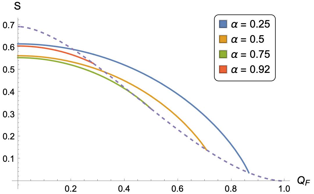
Figure 2: Plot of the entropy $S_{0}(\mathcal{Q}_{F})$ in the range $0\leq\mathcal{Q}_{F}<\sqrt{1-\alpha}$ for different values of $\alpha$, in the case $p=1$, $q=2$. The dashed line is the value of the entropy at the upper critical value of $\mathcal{Q}_{F}$ as $\alpha$ is varied.

Solutions for $\boldsymbol{p=q>1}$, $\boldsymbol{\alpha=1}$ and $\boldsymbol{\mathcal{E}\neq 0}$.

Similarly, plugging the explicit solution (3.39) for $\Delta_{\phi}(\mathcal{E})$ into the LW relation (3.100) we get

$$\mathcal{E}=-\frac{1}{2\pi p}\operatorname{arcsinh}\biggl{(}\frac{B}{\sqrt{2}\,\mathcal{Q}_{F}}\biggr{)}\;,\qquad\Delta_{\phi}=\frac{1}{4p}-\frac{1}{2\pi}\arcsin\biggl{[}\frac{\sqrt{2}\,|\mathcal{Q}_{F}|}{C}\sin\Bigl{(}\frac{\pi}{2p}\Bigr{)}\biggr{]}\;,$$ (3.107)

where we defined the following functions of $\mathcal{Q}_{F}$:

$$A =\cos\bigl{(}\tfrac{\pi}{2p}\bigr{)}\sqrt{\bigl{(}p^{2}-\mathcal{Q}_{F}^{2}\bigr{)}\rule{0.0pt}{6.99997pt}^{2}\cos^{2}\bigl{(}\tfrac{\pi}{2p}\bigr{)}+4p^{2}\mathcal{Q}_{F}^{2}}$$ (3.108)

$$B =\sqrt{\bigl{(}p^{2}-\mathcal{Q}_{F}^{2}\bigr{)}\cos^{2}\bigl{(}\tfrac{\pi}{2p}\bigr{)}+A}\;, C =\sqrt{p^{2}+\mathcal{Q}_{F}^{2}-\bigl{(}p^{2}-\mathcal{Q}_{F}^{2}\bigr{)}\sin^{2}\bigl{(}\tfrac{\pi}{2p}\bigr{)}+A}\;.$$

Note that $C^{2}-B^{2}=2\mathcal{Q}_{F}^{2}$. Evaluating the entropy function (3.104) on the solution we get

$$S_{0}=\log\Biggl{[}\frac{\cos\bigl{(}\frac{\pi}{2p}\bigr{)}\,\bigl{(}pC+\lvert\mathcal{Q}_{F}\rvert B\bigr{)}\,\bigl{(}C+\operatorname{sgn}(\mathcal{Q}_{F})B)^{\frac{\mathcal{Q}_{F}}{p}}}{2^{\frac{\mathcal{Q}_{F}}{2p}-\frac{1}{2}}\,|\mathcal{Q}_{F}|^{\frac{\mathcal{Q}_{F}}{p}}\,B^{2}}\Biggr{]}\;.$$ (3.109)

Figure 3 shows $S_{0}(\mathcal{Q}_{F})$ against $\mathcal{Q}_{F}$ for various values of $p=q$, and it is always positive.

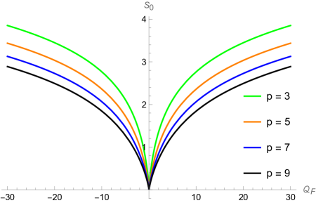
Figure 3: Plot of $S_{0}(\mathcal{Q}_{F})$ against $\mathcal{Q}_{F}$ for the solution in the cases $p=q=3,5,7,9$, $\mathcal{E}\neq 0$.

Solutions for $\boldsymbol{p=q>1}$ and $\boldsymbol{\mathcal{E}=0}$.

In this case, whenever $\alpha<\tan^{2}\bigl{(}\frac{\pi}{4p}\bigr{)}$ there are two acceptable conformal solutions (3.41) which coincide at $\alpha=\tan^{2}\bigl{(}\frac{\pi}{4p}\bigr{)}$. The only solution to the LW relation (3.100) is $\mathcal{Q}_{F}=0$. Evaluating (3.104) on (3.41) and with $\mathcal{Q}_{F}=0$ gives

$$\!S_{0}=\log\left[\frac{2\,\Bigl{(}(1-\alpha)\tan\bigl{(}\frac{\pi}{2p}\bigr{)}\pm\sqrt{(1-\alpha)^{2}\tan^{2}\bigl{(}\frac{\pi}{2p}\bigr{)}-4\alpha}\,\Bigr{)}^{\frac{1-\alpha}{2}}}{(1-\alpha)^{\frac{1-\alpha}{2}}\cos^{\alpha}\bigl{(}\frac{\pi}{2p}\bigr{)}\,\Bigl{(}(1+\alpha)\tan\bigl{(}\frac{\pi}{2p}\bigr{)}\pm\sqrt{(1-\alpha)^{2}\tan^{2}\bigl{(}\frac{\pi}{2p}\bigr{)}-4\alpha}\,\Bigr{)}^{\frac{1+\alpha}{2}}}\right]\!.\!$$ (3.110)

The signs above are correlated with the sign in (3.41). Figure 4 shows $S_{0}$ against $\alpha$ for $p=3$, and it is always positive. In addition, we see that the solution with the plus sign always has a higher entropy, and is expected to be the dominant saddle at large $N$.

Figure 4: Plot of $S_{0}$ against $\alpha\in\bigl{(}0,\tan^{2}\frac{\pi}{4p}\bigr{)}$ for the solutions in the case $p=q=3$, $\mathcal{E}=0$. The blue/black curves correspond to the solutions with a plus/minus sign in (3.41).

Solution at large $\boldsymbol{p}$.

One can check that the conformal parameters given in (3.58) solve the Schwinger–Dyson equation (3.29) up to $\mathcal{O}(p^{-3})$. Substituting the large $p$ values of $\Delta_{\eta}$ and $\Delta_{\phi}$ into (3.104), using (3.81) and

$$\cosh(2\pi\mathcal{E}_{\eta})+\cos(2\pi\Delta_{\eta}) =2\cosh^{2}(\pi q\mathcal{E})-\tfrac{\pi^{2}}{2p^{2}}+\mathcal{O}(p^{-4})\;,$$ (3.111)

$$\cosh(2\pi\mathcal{E}_{\phi})-\cos(2\pi\Delta_{\phi}) =2\sinh^{2}(\pi p\mathcal{E})+\mathcal{O}(p^{-4})\;,$$

reproduces the expansion in (3.69). This is a consistency check for the large $p$ computation.

4 Numerical results

In this section we present some results we obtained by numerically solving the Schwinger–Dyson equations. Our first goal is to check that the analytic approximations we carried out are sensible. Indeed we verify that the numerical solutions exhibit the conformal behaviour of equations (3.17) in the appropriate parameter region, and the non-conformal behavior of (3.84) outside that region. Second, we extract additional information which is analytically unreachable: we check that the zero-temperature limit of the entropy matches the prediction from the supersymmetric index and we estimate the Schwarzian coupling.

4.1 Summary of the numerical method

The SD equations can be solved numerically by adapting the method used in [6]. We discretize the interval $[0,\beta]$ into $M$ points, with $M$ a power of $2$. In frequency space we pick the $M$ fermionic and bosonic Matsubara frequencies with lowest absolute value, namely

$$\omega^{\rm f}_{k}=\frac{2\pi}{\beta}\biggl{(}k-\frac{M}{2}+\frac{1}{2}\biggr{)}\;,\qquad\omega^{\rm b}_{k}=\frac{2\pi}{\beta}\biggl{(}k-\frac{M}{2}+1\biggr{)}\;,\qquad k=0,\dots,M-1\;,$$ (4.1)

where the discretization is manifest because we take a finite number of frequencies. We transform between the two descriptions with Fast Fourier Transforms. We update each iteration with a weighing factor $x$, as in [6], for which we found $x=2/3$ to be a good general choice. Schematically,

$$G(\omega_{k})_{i}\rightarrow\Sigma(\tau_{k})_{i}=\Sigma_{\text{EOM}}\bigl{[}G(\tau_{k})_{i}\bigr{]}\rightarrow G(\omega_{k})_{i+1}=(1-x)G(\omega_{k})_{i}+xG_{\text{EOM}}\bigl{[}\Sigma(-\omega_{k})_{i}\bigr{]}.$$ (4.2)

We iterate until $\sum_{k}\bigl{\lvert}G(\omega_{k})_{i}-G(\omega_{k})_{i+1}\bigr{\rvert}^{2}$ is smaller than some precision goal. To begin the iteration, we take the free solution.

For small $\mu_{\phi}$ and finite $J$, the equation of motion for $G_{\bar{\phi}\phi}(\omega=0)$ is highly sensitive to numerical errors in $\Sigma_{\bar{\phi}\phi}(\omega=0)$. One possible workaround, proposed for example in [43], is to change the equation of motion for $G_{\bar{\phi}\phi}$ by replacing the parameter $\mu_{\phi}$ with $\rho$ so that $G_{\bar{\phi}\phi}(\omega=0)=\alpha\rho$. We replace the integro-differential equation for $G_{\bar{\phi}\phi}$ with

$$G_{\bar{\phi}\phi}\bigl{[}\Sigma(-\omega^{\text{b}}_{k})_{i}\bigr{]}=-\frac{\alpha\rho}{\rho\bigl{[}-i\omega^{\text{b}}_{k}+\Sigma_{\bar{\phi}\phi}(-\omega^{\text{b}}_{k})_{i}-\Sigma_{\bar{\phi}\phi}(0)_{i}\bigr{]}-1}\;.$$ (4.3)

One can then use the original equation of motion at the end to verify which value of $\mu_{\phi}$ is realized. In principle, one could take $\mu_{\phi}=\Sigma_{\bar{\phi}\phi}(0)+1/\rho$, however it is best to average the EOM in a window of frequency space. If one desires a specific value of $\mu_{\phi}$, this approach incurs a high additional numerical cost, since the solver must itself be iterated many times to carry out a bisection search or equivalent technique. Nevertheless, we found this to be a useful approach for those cases that are more numerically unstable, such as $(p,q)\neq(1,2)$.

4.2 Conformal behaviour for $\boldsymbol{(p,q)=(1,2)}$

In this section we focus on the case $(p,q)=(1,2)$. Numerically, this turns out to be the most accessible case. It is also of particular theoretical interest, as it is the closest choice to the quantum mechanical model in [29].

We first test that the conformal ansatz is realized at low energies. We take a solution with large $\beta J$, and we scan the numerical solutions to (3.22) for the best quadratic fit. These solutions are parameterised by $\mathcal{E}_{\eta}$, $\mathcal{E}_{\phi}$, $g_{\eta}$, and $g_{\phi}$. In principle, one could just fit $G_{\bar{\eta}\eta}$ and $G_{\bar{\phi}\phi}$, which can be beneficial since the auxiliary fields tend to converge slower to the conformal solution. However, we found that this results in less precise and less accurate estimates of the $\mathcal{E}$’s, so we fit the four bilocal fields together. Clearly, we must exclude from the fit the regions with $\tau$ close to $0$ and $\beta$, where the approximation is invalid and singular. Tipically we exclude $\bigl{\lvert}\frac{1}{2}-\frac{\tau}{\beta}\bigr{\rvert}>3/8$.

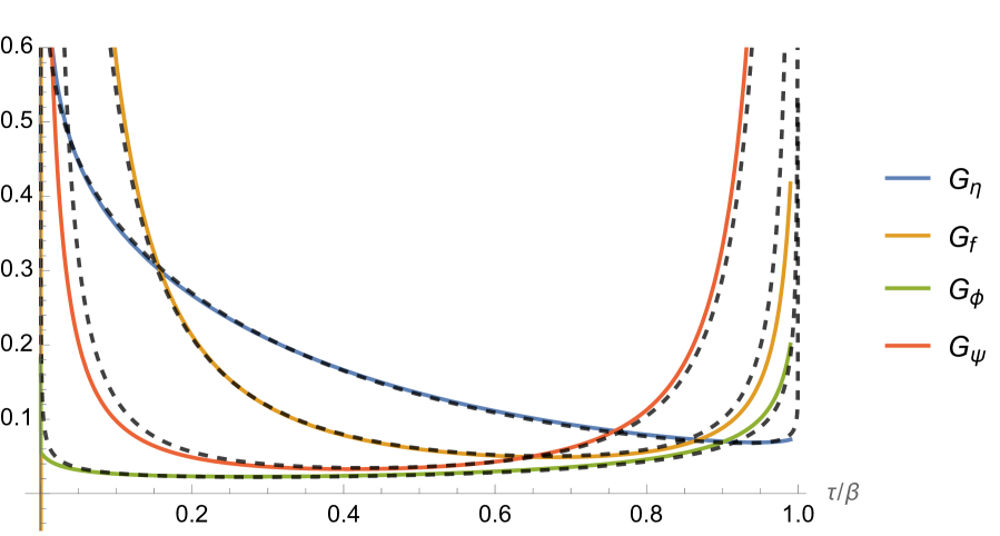
(a) $\bigl{(}\beta\mu_{\eta},\,\beta\mu_{\phi}\bigr{)}=(-2,\,1)$

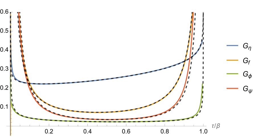
(b) $\bigl{(}\beta\mu_{\eta},\,\beta\mu_{\phi}\bigr{)}=(1,\,2)$

Figure 5: Two solutions for $\beta J=1000$, $\alpha=1/4$, $(p,q)=(1,2)$. The colored full lines are the numerical solution of the Schwinger–Dyson equations with $M=2^{18}$ points. The black dashed lines are a conformal solution for which the parameters $\mathcal{E}_{\eta,\mu}$ and $g_{\eta,\mu}$ have been fitted numerically. (a): Supersymmetric chemical potentials. (b): Non-supersymmetric.

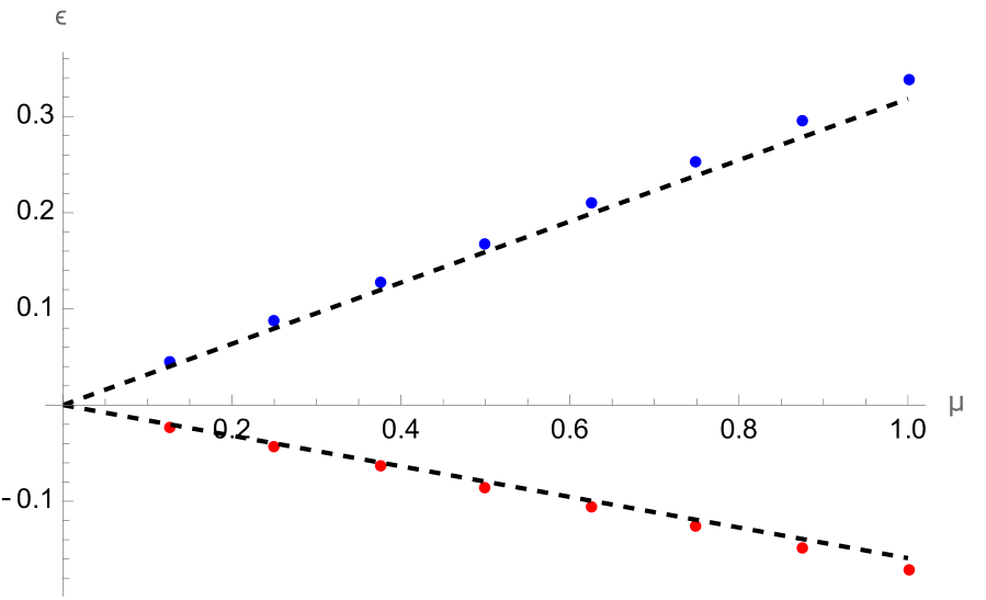
(a) $\bigl{(}\beta\mu_{\eta},\,\beta\mu_{\phi}\bigr{)}=(-2\mu,\,\mu)$

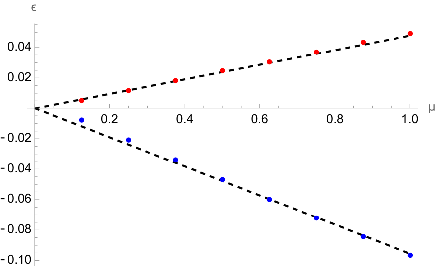
(b) $\bigl{(}\beta\mu_{\eta},\,\beta\mu_{\phi}\bigr{)}=(\mu,\,2\mu)$

Figure 6: Plot of $\mathcal{E}_{\eta}$ (blue points) and $\mathcal{E}_{\phi}$ (red points) as a function of $\mu$. The data was generated with $M=2^{20}$ points, $\beta J=600$, and $\alpha=1/5$. The dashed lines in each plot correspond to (4.4) (a: SUSY chemical potentials) and (4.5) (b: non-SUSY), respectively.

We present two illustrative examples in Figure 5. Clearly, the conformal solution is realized and it matches our proposed ansatz. For $(p,q)=(1,2)$ and supersymmetric chemical potentials, we verified numerically that, at sufficiently large $\beta J$, we have

$$2\pi\mathcal{E}_{\eta}\,\simeq\,-\beta\mu_{\eta}=2\beta\mu_{\phi}\;,\qquad\qquad 2\pi\mathcal{E}_{\phi}\,\simeq\,-\beta\mu_{\phi}\;,$$ (4.4)

which matches the expectation from the supersymmetric index. This suggests that, even in the deep IR, SUSY is at most lightly broken at small temperatures. For other choices of chemical potentials, we also find a linear relation at low temperatures. The ansatz

$$2\pi\mathcal{E}_{\eta}\,\simeq\,-\biggl{(}1-\frac{2\alpha}{5}\biggr{)}\beta\mu_{\eta}+\frac{4\alpha}{5}\beta\mu_{\phi}\;,\qquad 2\pi\mathcal{E}_{\phi}\,\simeq\,\frac{1}{2}\biggl{(}1-\frac{2\alpha}{5}\biggr{)}\beta\mu_{\eta}-\frac{2\alpha}{5}\beta\mu_{\phi}$$ (4.5)

was numerically successful for large $\beta J$ and finite chemical potentials well below the critical value, testing with different values of $\alpha$. We plot a supersymmetric and a non-supersymmetric example in Figure 6. This ansatz has the curious property of being supersymmetric irrespectively of the chemical potentials, suggesting an emergent IR supersymmetry. When fitting the low energy behaviour, $\Delta_{\phi,\eta}$ and $g_{\phi,\eta}$ also satisfy the respective supersymmetry constraints within $1\%-5\%$ at $\beta J$ between $200$ and $600$. This ansatz was further confirmed when comparing the numerical values of the charge and entropy to the Luttinger–Ward relation and the zero-temperature entropy for non-supersymmetric cases in Section 4.3. However, we note that one expects, for physical fields at fixed $\mathcal{Q}_{\eta,\phi}$, to have

$$\mu_{I}(\mathcal{Q}_{\eta},\mathcal{Q}_{\phi},T)=\mu_{0,I}(\mathcal{Q}_{\eta},\mathcal{Q}_{\phi})+2\pi\mathcal{E}_{I}(\mathcal{Q}_{\eta},\mathcal{Q}_{\phi})T+\ldots\;,$$ (4.6)

see for instance [44, 45, 12]. Here the index $I=\eta,\phi$ labels the $\mathrm{U}(1)$ symmetries. Since we work at fixed $\mu$ and the function $\mathcal{Q}_{I}(\mu)$ is a priori complicated, eqn. (4.5) might be the linearized behaviour of a more intricate function $\mu_{0,I}\bigl{(}\mathcal{Q}_{\eta}(\mu_{\eta},\mu_{\phi}),\,\mathcal{Q}_{\phi}(\mu_{\eta},\mu_{\phi})\bigr{)}$.

4.3 Charge and entropy for $\boldsymbol{(p,q)=(1,2)}$

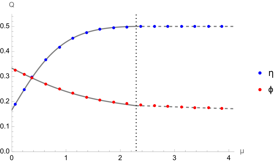
(a) $\alpha=1/3$

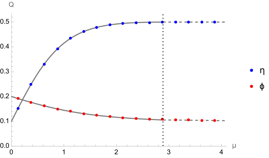
(b) $\alpha=1/5$

Figure 7: We plot $\mathcal{Q}_{\eta}$ (blue points) and $\mathcal{Q}_{\phi}$ (red points) as a function of $\mu_{F}$. The data was generated with $M=2^{18}$ points, $\beta J=200$ and $(\beta\mu_{\eta},\beta\mu_{\phi})=(-2\mu,\mu)$. The gray full line is the Luttinger–Ward formula (4.7), assuming (4.4). The gray dashed lines are the continuations in (4.8). The vertical dotted line is the value $\mu_{F}$ for which $\mathcal{E}_{*}$ is reached.

An important check of the conformal ansatz is the Luttinger–Ward relation between $\mathcal{E}$ and $\mathcal{Q}$, which we presented in Section 3.7. As previously noted, the Luttinger–Ward calculation determines $\mathcal{Q}(\mathcal{E})$ up to undetermined constants, which we fixed exploiting the index in (3.103). Numerically, we can verify these constants to be:

$$\mathcal{Q}_{\eta} =\mathfrak{q}_{-}(\mathcal{E}_{\eta},\Delta_{\eta})+(1-p)\,\mathfrak{q}_{+}(\mathcal{E}_{f},\Delta_{f})-\alpha p\,\mathfrak{q}_{-}(\mathcal{E}_{\psi},\Delta_{\psi})+\frac{\alpha p}{2}\;,$$ (4.7)

$$\mathcal{Q}_{\phi} =\alpha\,\mathfrak{q}_{+}(\mathcal{E}_{\phi},\Delta_{\phi})+\alpha(1-q)\,\mathfrak{q}_{-}(\mathcal{E}_{\psi},\Delta_{\psi})-q\,\mathfrak{q}_{+}(\mathcal{E}_{f},\Delta_{f})+\frac{\alpha q}{2}\;,$$

where the function $\mathfrak{q}$ is given in (3.80). This matches the index prediction (3.103). We note that the charges do not vanish when $\mu_{\eta,\phi}\rightarrow 0$, which is supported by the numerics, as can be seen in Figure 7. The charges also converge very quickly to their low-temperature limit, since they depend on $\beta J$ through $\mathcal{E}$. Thus we can take $\beta J$ to be large and assume (4.4).

In the superconformal solution, as we take $\mathcal{E}$ close to $\mathcal{E}_{*}(\alpha)$ defined in (3.33), we approach the phase transition discussed in Section 3.4. In order to avoid working with $\mathcal{E}$ which is numerically more indirect, we label as $\beta\mu_{\phi}^{*}=2\operatorname{arccosh}\bigl{(}\alpha^{-\frac{1}{2}}\bigr{)}$ the critical chemical potential, which follows from (4.4).

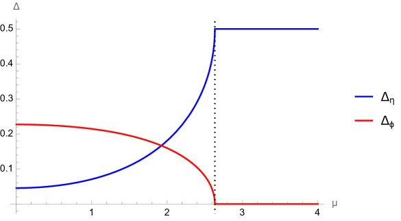
Figure 8: We plot $\Delta_{\eta}$ and $\Delta_{\phi}$ for $\alpha=1/4$ and $(\beta\mu_{\eta},\beta\mu_{\phi})=(-2\mu,\mu)$, assuming (4.4). The data was generated by solving (3.29) numerically. The vertical dotted line is at the value of $\mu$ for which $\mathcal{E}_{*}$ is reached.

Recall that, as $\mathcal{E}\rightarrow\mathcal{E}_{*}$, the conformal dimensions converge to $\Delta_{\eta}=1/2$ and $\Delta_{\phi}=0$, see Figure 8. This is a solution — albeit a trivial one — to the consistency equations (3.23), or equivalently (3.29), for any value of $\mathcal{E}$. Focusing only on the consistency equations, the absence of other nearby solutions for the conformal dimensions when $\mathcal{E}>\mathcal{E}_{*}$ suggests that the would-be conformal solution should have these marginal values. While, technically, this fact renders the conformal approximation no longer valid, since the kinetic and interacting terms are of the same order in $\omega$, we can conjecturally extend the Luttinger–Ward relation by plugging the fixed dimensions in. We conjecture

$$\mathcal{Q}_{\eta}=\frac{1}{2}\;,\qquad\qquad\mathcal{Q}_{\phi}=1-\coth(\beta\mu_{F})+\frac{\alpha}{2}\coth\biggl{(}\frac{\beta\mu_{F}}{2}\biggr{)}\;.$$ (4.8)

As we can see in the dashed line in Figure 7, the numerical results do not deviate significantly from such an analytic continuation.

We can further combine this result with (3.106) in order to obtain a zero-temperature analytic prediction for the entropy as a function of the flavour chemical potential, within the conformal phase and, conjecturally, beyond. We use (3.86) to calculate the entropy numerically at each finite temperature, and then we take $\beta J\rightarrow\infty$ with $\beta\mu$ fixed.

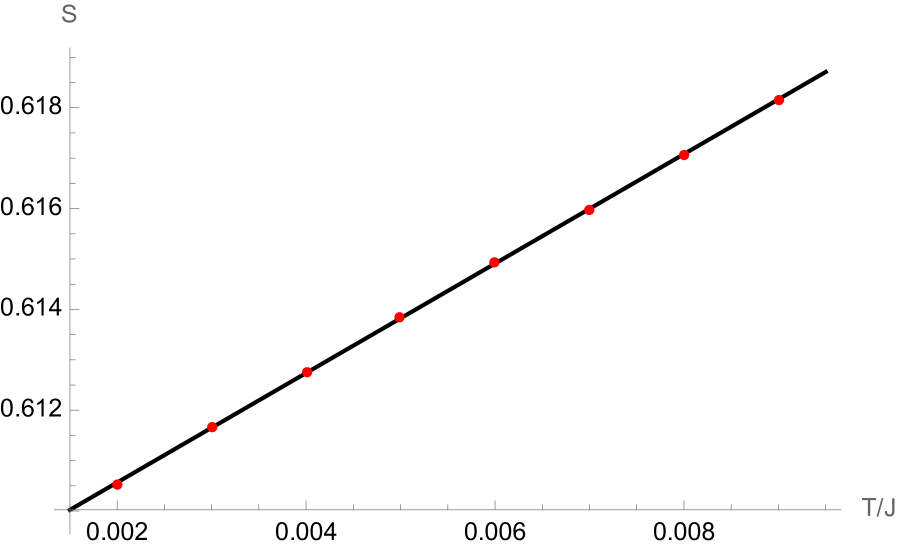
(a) $\alpha=\frac{1}{4}$, $\mu=0.125$, $r=0$, $M=2^{22}$

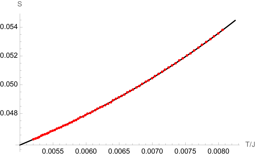
(b) $\alpha=\frac{1}{4}$, $\mu=2.58$, $r=3$, $M=2^{24}$

Figure 9: We plot two examples of the extrapolation of the zero-temperature entropy for $(\beta\mu_{\eta},\beta\mu_{\phi})=(-2\mu,\mu)$. In plot 9(a) we take a small value of $\mu$ for which it suffices to fit with a line, allowing us also to estimate the Schwarzian coupling. Meanwhile, in plot 9(b) we take a value of $\mu$ close to the phase transition. Instead of fitting the points directly, we fit the third Richardson transform with the ansatz (4.10). Here $M$ is the number of points in the discretized Schwinger–Dyson equation.

For the extrapolation to zero temperature, the precision strongly depends on how close to the phase transition we are. For values of the chemical potential sufficiently below $\beta\mu_{\phi}^{*}$, it suffices to probe values of $\beta J$ between $50$ and $500$ and use a polynomial fit to extract the constant term, as can been seen in Figure 9(a). The error is estimated by dropping points at both ends of the sample. The resulting extrapolation of the zero-temperature entropy are the red dots in Figure 10. However, as we move closer to the critical point, this extrapolation becomes harder. The main limiting factor is that we cannot probe arbitrarily low temperatures due finite-size effects and numerical instabilities. Furthermore, if we assume that the entropy behaves as

$$S(T)\,\approx\,S_{0}+g_{\text{Sch}}(\beta J)^{-1}+g_{\gamma}(\beta J)^{-\gamma}+\ldots\;,$$ (4.9)

what we observe numerically (as well as in the analysis of the spectrum in Section 5) is that $\gamma$ becomes close to $1$. Thus, we generate points at integer values of $\beta J$ between $100$ and $400$ and then take one or more Richardson transforms, see [46, 47]. After the $r$-th Richardson transform, we expect to converge to $S_{0}$ as

$$\bigl{[}S(T)\bigr{]}_{r}\,\approx\,S_{0}+g_{\gamma,r}(\beta J)^{-\gamma}+g_{r}(\beta J)^{-(1+r)}+\ldots\;.$$ (4.10)

Fitting the form (4.10) for all the constants is more reliable at low temperature than (4.9) since the exponents are more distinct, and we estimate the numerical error by varying the points included in the fit and the order $r$ of the Richardson transform. We used this strategy for the light blue points in Figure 10, with a step of $10$ for those on the left and a step of $4$ for those on the right (a smaller step increases the convergence of the Richardson acceleration). Lastly, for points very close to the critical point the convergence to $S_{0}$ is particularly slow, so we considered only points with $\beta J$ between $200$ and $400$ with a step of $2$. These are the dark blue points in Figure 10. The error is estimated by varying the degree of the Richardson transform and by comparing with the previous method, taking the largest estimate. An example of such a fit is given in Figure 9(b). The exponent $\gamma$ in (4.9) seems to be close to $1$ at the transition point, but unfortunately the precision attainable with our points is not enough to extract meaningful estimates, including whether it is smaller or larger than $1$.

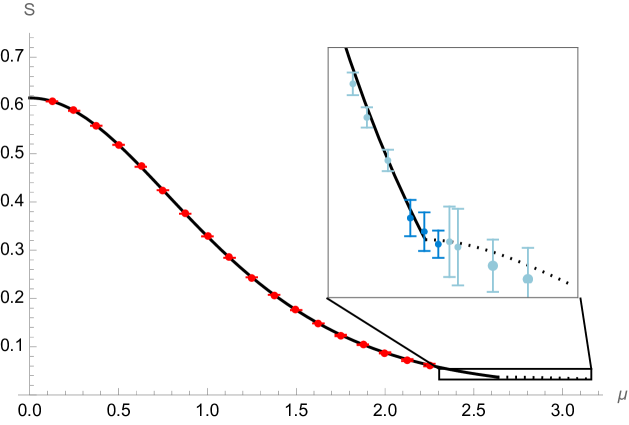
Figure 10: Plot of the zero-temperature entropy $S_{0}$ as a function of the chemical potentials $(\beta\mu_{\eta},\beta\mu_{\phi})=(-2\mu,\mu)$ at $\alpha=1/4$. The red dots were generated with $2^{22}$ points, $\beta J$ spanning from $200$ to $1000$, and the entropy was obtained with simple linear extrapolation. The light blue and dark blue dots were generated with $2^{23}$ and $2^{24}$ points, respectively, with $\beta J$ spanning from $100$ to $400$, and extrapolated using the Richardson-transform fit described in eqn. (4.10). The black line is the prediction from combining the index and the Luttinger–Ward formula (4.7), while the dashed line uses the index and the continuation (4.8).

Unfortunately, $\beta J\sim 500$ is still slowly converging to the low-temperature behaviour and the above techniques have limited success in isolating $S_{0}$. Furthermore, the results are sensitive to small changes in the extrapolation method, which we attempt to capture with the error estimates in Figure 10, but which are likely underestimated. With these significant caveats, what we can at best observe is that, in Figure 10, the kink that follows from extrapolating $\mathcal{Q}_{F}(\mu)$ with (4.8) seems to be close to the numerical results. This could suggest some form of second-order phase transition. However, note that this would-be kink only appears when working at fixed chemical potential, while at fixed charge we can just apply (3.106) directly, which is smooth.

$$\begin{array}[]{c | cc | cc}\hline\cr\hline\cr&\lx@intercol\hfil\beta\mu_{\phi}=1/8\hfil\lx@intercol\vrule\lx@intercol&\lx@intercol\hfil\beta\mu_{\phi}=3/2\hfil\lx@intercol\\ \alpha&\mathcal{Q}_{F}&g_{\text{Sch}}&\mathcal{Q}_{F}&g_{\text{Sch}}\\ \hline\cr 1/4&0.1087&1.09\pm 0.03&0.7920&1.09\pm 0.01\\ 1/5&0.1119&0.97\pm 0.03&0.8147&0.96\pm 0.01\\ 1/6&0.1140&0.90\pm 0.03&0.8298&0.90\pm 0.02\\ 1/7&0.1155&0.87\pm 0.04&0.8405&0.86\pm 0.02\\ \hline\cr\hline\cr\end{array}$$

Table 2: Estimates of the Schwarzian coupling, for $(\beta\mu_{\eta},\beta\mu_{\phi})=(-2\mu,\mu)$.

For chemical potentials sufficiently lower than the transition point, we can also extract the coefficient of the linear term in $T$ from the entropy, which should be proportional to the Schwarzian coupling. However, as we move closer to the phase transition, the linear behaviour is less clear as it seems to require even lower temperatures. We show some of the estimates of $g_{\text{Sch}}$ for different values of $\mathcal{Q}_{F}$ in Table 2.

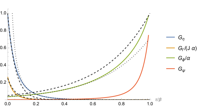
Figure 11: Solutions for $\beta J=400$, $\alpha=1/4$, $(p,q)=(1,2)$, $(\beta\mu_{\eta},\beta\mu_{\phi})=(-6,3)$. The colored full lines are the numerical solution to the Schwinger–Dyson equations with $2^{22}$ points. The black dashed lines are the zero-temperature prediction (3.84). The dotted lines are the prediction from the conformal ansatz with $\Delta_{\eta}=\frac{1}{2}$, $\Delta_{\phi}=0$, $\mathcal{E}_{\eta,\phi}$ as in (4.4), and $g_{\eta,\phi}$ fitted numerically. In the conformal solution $G_{\bar{f}f}=G_{\bar{\psi}\psi}=0$.

As for the solutions themselves, at $\beta\mu_{\phi}>\beta\mu_{\phi}^{*}$ they seem to interpolate between the conformal solution and the exponential behaviour of the non-conformal solution (3.82), as we illustrate in Figure 11. For $\tau$ in the middle of the interval (the IR regime), we see that a conformal ansatz with $\Delta_{\eta}=1/2$ and $\Delta_{\phi}=0$ is a good approximation of the physical fields $\eta,\phi$ (for the auxiliary fields $f,\psi$, the ansatz gives $0$), while at $\tau$ closer to $0$ and $\beta$ the non-conformal solution is a better match. As we take $\beta\mu_{F}\rightarrow\infty$, the solution seems to converge to (3.82), which analytically corresponds to the case $\beta\rightarrow\infty$ and $\mu$ finite. As shown in Figure 12, we can match $G_{\bar{\eta}\eta}$, $G_{\bar{f}f}$, and $G_{\bar{\phi}\phi}$ with their zero-temperature limit. $G_{\bar{\psi}\psi}$ vanishes at zero temperature, so we observe that it is dominated by the subleading contribution, which we did not establish analytically.

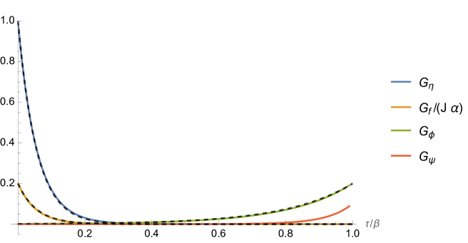
Figure 12: Solutions for $\beta J=400$, $\alpha=1/4$, $(p,q)=(1,2)$, $(\beta\mu_{\eta},\beta\mu_{\phi})=(-10,5)$. The colored full lines are the numerical solution to the Schwinger–Dyson equations with $2^{18}$ points. The black dashed lines are the zero-temperature prediction (3.84).

4.3.1 Entropy for non-supersymmetric solutions

One can also solve the Schwinger–Dyson equations for non-supersymmetric chemical potentials. Using a similar extrapolation as before, one can then obtain the zero-temperature entropy. Since we empirically found a supersymmetric low-energy behaviour in (4.5), we can conjecturally compare the non-supersymmetric zero-temperature entropy with the entropy from the $\mathcal{I}$-extremization using the values of $\mathcal{E}$ in (4.5). In Figure 13 we plot such an example. The theoretical prediction seems compatible with the numerical result within the extrapolation error for smaller values of $\mu_{\eta}$ and $\mu_{\phi}$. Unfortunately, the numerical iteration is noticeably more unstable for non-supersymmetric potentials, and thus we could neither probe a wider range of chemical potentials nor work with greater precision.

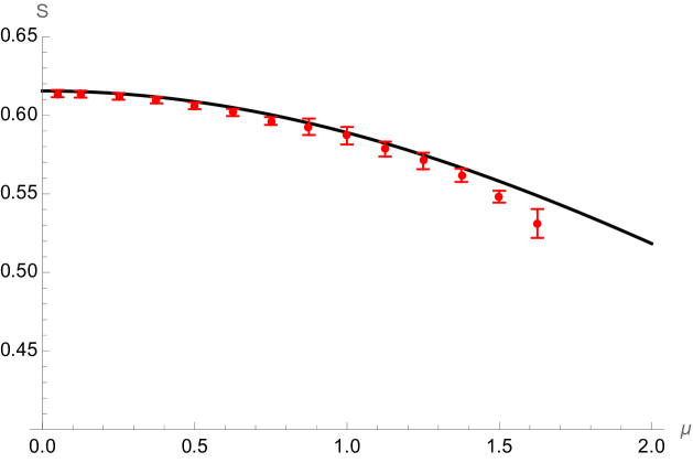
Figure 13: Plot of the zero-temperature entropy $S_{0}$ as a function of the chemical potentials $(\beta\mu_{\eta},\beta\mu_{\phi})=(\mu,2\mu)$ at $\alpha=\frac{1}{4}$. The red dots were generated with $2^{23}$ points, $\beta J$ spanning from $10$ to $200$, and linear extrapolation of the entropy. The black line is the prediction obtained from the index, the Luttinger–Ward formula (4.7), and the ansatz (4.5).

Even within the small band of values of $\mu$ probed numerically, these results are surprising. They reinforce the SUSY IR behaviour found in (4.5). Unlike the check of Figure 6, this test does not rely on fitting $\mathcal{E}_{\phi,\eta}$ at late $\tau$, which is a delicate task. So this figure is independent evidence of the emergent SUSY. Due to numerical limitations, we cannot however ascertain whether this behaviour is valid only for small values of $\mu$ or due to numerical errors.

4.4 Results for other values of $\boldsymbol{(p,q)}$

Solving the Schwinger–Dyson equation for values of $(p,q)$ other than $(1,2)$ turns out to be numerically more unstable. The standard prescription, when it stabilises, often lands on the exponential-like non-conformal solutions. We can use the prescription (4.3) to find conformal-like solutions, but this makes the study of supersymmetric solutions much more costly since it requires iterating for many values of $\rho$, since for each value of $\mu_{\eta}$ it is a priori unknown which value of $\rho$ corresponds to the supersymmetric value of $\mu_{\phi}$. In Figure 14 we show some examples of the conformal solution being realized for $p=q=3$. In this case we can even compare a conformal and non-conformal solution for the same values of $(\beta\mu_{\eta},\beta\mu_{\phi})$, obtained with (4.2) instead.

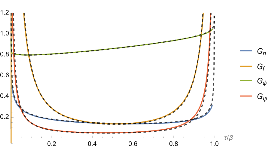
(a) Conformal-like solution

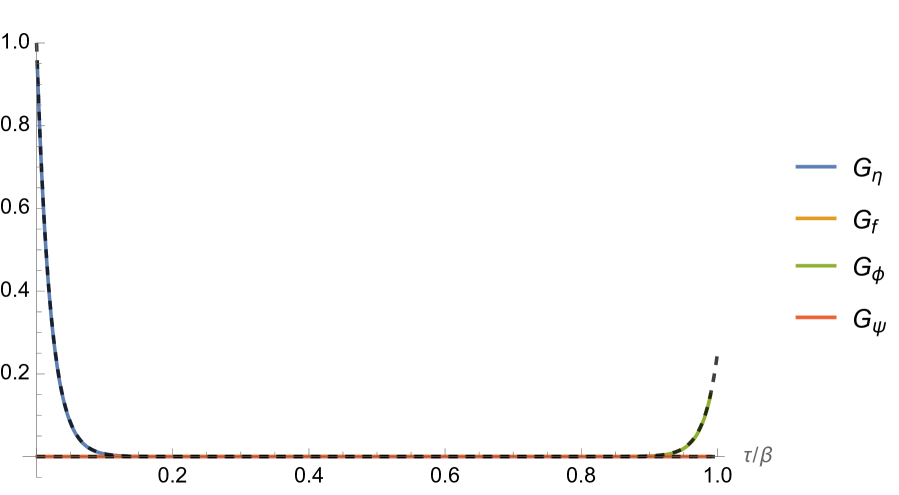
(b) Exponential-like solution

Figure 14: Two solutions for $\beta J=450$, $\alpha=\frac{1}{4}$, $(p,q)=(3,3)$, and $(\beta\mu_{\eta},\beta\mu_{\phi})=(-30,30)$. The colored full lines are the numerical solution to the Schwinger–Dyson equations with $2^{20}$ points, using (4.3) on the left and the standard approach on the right. (a): The black dashed lines are a fit of the conformal ansatz. (b): The black dashed lines represent the zero-temperature non-conformal solution (3.84).

5 Spectrum of low-lying operators

In order to understand the IR dynamics of the model, we find the spectrum of physical excitations around conformal solutions. For simplicity, we present the full derivation only for superconformal solutions, while we describe the non-supersymmetric case at the end.

5.1 Expanding the action

In order to derive the spectrum, we expand the fields around solutions of the equations of motion, and then diagonalize the quadratic fluctuations. In superspace, one expands the bilocal fields around the superconformal solutions as

$$\mathcal{G}_{\mathcal{Y}}(T_{1},T_{2}) =G^{*}_{\bar{\eta}\eta}(T_{12})+\frac{1}{N^{\frac{1}{2}}}\delta\mathcal{G}_{\mathcal{Y}}(T_{1},T_{2})\,, \mathcal{G}_{\Phi}(T_{1},T_{2}) =G^{*}_{\bar{\phi}\phi}(T_{12})+\frac{1}{N^{\frac{1}{2}}}\delta\mathcal{G}_{\Phi}(T_{1},T_{2})$$ (5.1)

$$\Sigma_{\mathcal{Y}}(T_{1},T_{2}) =\Sigma^{*}_{\bar{f}f}(T_{12})+\frac{1}{N^{\frac{1}{2}}}\delta\Sigma_{\mathcal{Y}}(T_{1},T_{2})\,, \Sigma_{\Phi}(T_{1},T_{2}) =\Sigma^{*}_{\bar{\psi}\psi}(T_{12})+\frac{1}{N^{\frac{1}{2}}}\delta\Sigma_{\Phi}(T_{1},T_{2})\,.$$ (5.2)

Here $G^{*}$ and $\Sigma^{*}$ indicate the superconformal solutions. Due to supersymmetry, the bilocal superfields are determined by their lowest components as in (3.25). When expanding the action (3.6), the terms containing $\delta\Sigma$’s at quadratic order are:

$$\frac{1}{2}\int\!d^{2}T_{2}\,d^{2}\overline{T}_{1}\,d^{2}T_{4}\,d^{2}\overline{T}_{3}\;\delta\Sigma(T_{1},T_{2})^{\sf{T}}\begin{pmatrix}-G^{*}_{\bar{\eta}\eta}G^{*}_{\bar{\eta}\eta}&0\\ 0&\frac{1}{\alpha}G^{*}_{\bar{\phi}\phi}G^{*}_{\bar{\phi}\phi}\end{pmatrix}\!(T_{14},T_{32})\;\delta\Sigma(T_{3},T_{4})\\ +\frac{1}{2}\int\!d^{2}T_{2}\,d^{2}\overline{T}_{1}\;\delta\mathcal{G}(T_{1},T_{2})^{\sf{T}}\,\delta\Sigma(T_{1},T_{2})+\frac{1}{2}\int\!d^{2}T_{2}\,d^{2}\overline{T}_{1}\;\delta\Sigma(T_{1},T_{2})^{\sf{T}}\,\delta\mathcal{G}(T_{1},T_{2})\;,$$ (5.3)

where we defined $\delta\Sigma(T_{1},T_{2})=\big{(}\begin{smallmatrix}\delta\Sigma_{\mathcal{Y}}\\ \delta\Sigma_{\Phi}\end{smallmatrix}\big{)}(T_{1},T_{2})$ and $\delta\mathcal{G}(T_{1},T_{2})=\big{(}\begin{smallmatrix}\delta\mathcal{G}_{\mathcal{Y}}\\ \delta\mathcal{G}_{\Phi}\end{smallmatrix}\big{)}(T_{1},T_{2})$. In the matrix on the first line, $T_{14}$ and $T_{32}$ are the arguments of the first and second $G^{*}$, respectively. Since we are interested in the action for $\delta\mathcal{G}$ to leading order in $N$, it is sufficient to integrate out $\delta\Sigma$ classically. Combining the result with terms in the action involving $\delta\mathcal{G}$ only, we get the quadratic terms

$$-\frac{1}{2}\int\!d^{2}T_{2}\,d^{2}\overline{T}_{1}\,d^{2}T_{4}\,d^{2}\overline{T}_{3}\;\delta\mathcal{G}(T_{1},T_{2})^{\sf{T}}\,\mathcal{F}_{0}^{-1}\cdot\bigl{[}\mathbbm{1}-\mathcal{K}\bigr{]}(T_{1},T_{2};T_{3},T_{4})\;\delta\mathcal{G}(T_{3},T_{4})\;.$$ (5.4)

The operator $\mathcal{K}$, which we call the superspace kernel, is given by:

$$\mathcal{K}(T_{1},T_{2};T_{3},T_{4})\equiv\begin{pmatrix}\mathcal{K}_{\mathcal{Y}\mathcal{Y}}(T_{1},T_{2};T_{3},T_{4})&\mathcal{K}_{\mathcal{Y}\Phi}(T_{1},T_{2};T_{3},T_{4})\\ \mathcal{K}_{\Phi\mathcal{Y}}(T_{1},T_{2};T_{3},T_{4})&\mathcal{K}_{\Phi\Phi}(T_{1},T_{2};T_{3},T_{4})\end{pmatrix}\qquad\qquad$$ (5.5)

$$\mathcal{K}_{\mathcal{Y}\mathcal{Y}}(T_{1},T_{2};T_{3},T_{4}) =\frac{(p-1)J}{q}\,G^{*}_{\bar{\eta}\eta}(T_{34})^{p-2}\,G^{*}_{\bar{\phi}\phi}(T_{34})^{q}\,G^{*}_{\bar{\eta}\eta}(T_{14})\,G^{*}_{\bar{\eta}\eta}(T_{32})\;,$$ (5.6)

$$\mathcal{K}_{\mathcal{Y}\Phi}(T_{1},T_{2};T_{3},T_{4}) =J\,G^{*}_{\bar{\eta}\eta}(T_{34})^{p-1}\,G^{*}_{\bar{\phi}\phi}(T_{34})^{q-1}\,G^{*}_{\bar{\eta}\eta}(T_{14})\,G^{*}_{\bar{\eta}\eta}(T_{32})\;,$$

$$\mathcal{K}_{\Phi\mathcal{Y}}(T_{1},T_{2};T_{3},T_{4}) =-\frac{J}{\alpha}\,G^{*}_{\bar{\phi}\phi}(T_{34})^{q-1}\,G^{*}_{\bar{\eta}\eta}(T_{34})^{p-1}\,G^{*}_{\bar{\phi}\phi}(T_{14})\,G^{*}_{\bar{\phi}\phi}(T_{32})\;,$$

$$\mathcal{K}_{\Phi\Phi}(T_{1},T_{2};T_{3},T_{4}) =-\frac{(q-1)J}{\alpha p}\,G^{*}_{\bar{\phi}\phi}(T_{34})^{q-2}\,G^{*}_{\bar{\eta}\eta}(T_{34})^{p}\,G^{*}_{\bar{\phi}\phi}(T_{14})\,G^{*}_{\bar{\phi}\phi}(T_{32})\;.$$

After plugging the supersymmetric conformal ansatz (3.16) in, we obtain

$$\mathcal{K}_{\mathcal{Y}\mathcal{Y}} =\frac{(p-1)g_{\eta}^{p}g_{\phi}^{q}J}{q}\,G_{-}(T_{14};\Delta_{\eta},\mathcal{E}_{\eta})\,G_{-}(T_{32};\Delta_{\eta},\mathcal{E}_{\eta})\,G_{-}\bigl{(}T_{34};\tfrac{1}{2}-2\Delta_{\eta},-2\mathcal{E}_{\eta}\bigr{)}\,,$$ (5.7)

$$\mathcal{K}_{\mathcal{Y}\Phi} =g_{\eta}^{p+1}g_{\phi}^{q-1}J\,G_{-}(T_{14};\Delta_{\eta},\mathcal{E}_{\eta})\,G_{-}(T_{32};\Delta_{\eta},\mathcal{E}_{\eta})\,G_{+}\bigl{(}T_{34};\tfrac{1}{2}-\Delta_{\eta}-\Delta_{\phi},-\mathcal{E}_{\eta}-\mathcal{E}_{\phi}\bigr{)}\,,$$

$$\mathcal{K}_{\Phi\mathcal{Y}} =-\frac{g_{\eta}^{p-1}g_{\phi}^{q+1}J}{\alpha}\,G_{+}(T_{14};\Delta_{\phi},\mathcal{E}_{\phi})\,G_{+}(T_{32};\Delta_{\phi},\mathcal{E}_{\phi})\,G_{+}\bigl{(}T_{34};\tfrac{1}{2}-\Delta_{\eta}-\Delta_{\phi},-\mathcal{E}_{\eta}-\mathcal{E}_{\phi}\bigr{)}\,,$$

$$\mathcal{K}_{\Phi\Phi} =-\frac{(q-1)g_{\eta}^{p}g_{\phi}^{q}J}{\alpha p}\,G_{+}(T_{14};\Delta_{\phi},\mathcal{E}_{\phi})\,G_{+}(T_{32};\Delta_{\phi},\mathcal{E}_{\phi})\,G_{-}\bigl{(}T_{34};\tfrac{1}{2}-2\Delta_{\phi},-2\mathcal{E}_{\phi}\bigr{)}\,.$$

We also defined the matrix $\mathcal{F}_{0}$ as

$$\mathcal{F}_{0}(T_{1},T_{2};T_{3},T_{4})\equiv\begin{pmatrix}-G^{*}_{\bar{\eta}\eta}G^{*}_{\bar{\eta}\eta}&0\\ 0&\frac{1}{\alpha}G^{*}_{\bar{\phi}\phi}G^{*}_{\bar{\phi}\phi}\end{pmatrix}(T_{14},T_{32})\;.$$ (5.8)

From (5.4) we see that the spectrum is determined by the zeros of the kinetic operator $\mathbbm{1}-\mathcal{K}$, which is determined by the eigenvalue equation

$$\delta\mathcal{G}(T_{1},T_{2})=\int\!d^{2}\overline{T}_{3}\,d^{2}T_{4}\;\mathcal{K}(T_{1},T_{2};T_{3},T_{4})\;\delta\mathcal{G}(T_{3},T_{4})\;.$$ (5.9)

5.1.1 Deriving the spectral problem from the Schwinger–Dyson equations

A shortcut to obtain the same eigenvalue equation is to expand the Schwinger–Dyson equations around superconformal solutions. The eqns. (3.7), (3.8), (3.10) can be recast as

$$J\int\!d^{2}T_{4}\;\mathcal{G}_{\mathcal{Y}}(T_{34})^{p-1}\,\mathcal{G}_{\Phi}(T_{34})^{q-1}\begin{pmatrix}\mathcal{G}_{\mathcal{Y}}(T_{14})\,\mathcal{G}_{\Phi}(T_{34})\\ \mathcal{G}_{\Phi}(T_{14})\,\mathcal{G}_{\mathcal{Y}}(T_{34})\end{pmatrix} =\begin{pmatrix}q\,\overline{\delta}^{2}(T_{1},T_{3})\\ -p\,\alpha\,\overline{\delta}^{2}(T_{1},T_{3})\end{pmatrix}\,,$$ (5.10)

$$J\int\!d^{2}\overline{T}_{3}\;\mathcal{G}_{\mathcal{Y}}(T_{34})^{p-1}\,\mathcal{G}_{\Phi}(T_{34})^{q-1}\begin{pmatrix}\mathcal{G}_{\mathcal{Y}}(T_{32})\,\mathcal{G}_{\Phi}(T_{34})\\ \mathcal{G}_{\Phi}(T_{32})\,\mathcal{G}_{\mathcal{Y}}(T_{34})\end{pmatrix} =\begin{pmatrix}q\,\delta^{2}(T_{4},T_{2})\\ -p\,\alpha\,\delta^{2}(T_{4},T_{2})\end{pmatrix}\,.$$

The kinetic terms in (3.8) and (3.10) have been justifiably neglected in the IR. The upper component of the first equation in (5.10) can be expanded to linear order in $\delta\mathcal{G}$ as:

$$\frac{J}{q}\int\!d^{2}T_{4}\biggl{[}(p-1)G^{*}_{\bar{\eta}\eta}(T_{34})^{p-2}G^{*}_{\bar{\phi}\phi}(T_{34})^{q}G^{*}_{\bar{\eta}\eta}(T_{14})\delta\mathcal{G}_{\mathcal{Y}}(T_{3},T_{4})+{}$$ (5.11)

$$\;\;+qG^{*}_{\bar{\eta}\eta}(T_{34})^{p-1}G^{*}_{\bar{\phi}\phi}(T_{34})^{q-1}G^{*}_{\bar{\eta}\eta}(T_{14})\delta\mathcal{G}_{\Phi}(T_{3},T_{4})+G^{*}_{\bar{\eta}\eta}(T_{34})^{p-1}G^{*}_{\bar{\phi}\phi}(T_{34})^{q}\delta\mathcal{G}_{\mathcal{Y}}(T_{1},T_{4})\biggr{]}=0\,.$$

Multiplying by $G^{*}_{\bar{\eta}\eta}(T_{32})$, integrating over $T_{3}$, and using the second equation in (5.10), we obtain the upper component of (5.9). An analogous equation for $\mathcal{G}_{\Phi}$ can be obtained from the bottom component of the first equation in (5.10), so reproducing the full (5.9).

5.1.2 4-point functions in the large $\boldsymbol{N}$ limit

With the quadratic action (5.4) we can also derive 4-point functions to order $\mathcal{O}(\frac{1}{N})$. After the disorder average, the 4-point functions we can compute are those expressed in terms of bilocal fields, which we group into a matrix:

$$\frac{1}{N^{2}}\biggl{\langle}\,\begin{matrix}\overline{\mathcal{Y}}_{a}\mathcal{Y}_{a}\overline{\mathcal{Y}}_{b}\mathcal{Y}_{b}&\overline{\mathcal{Y}}_{a}\mathcal{Y}_{a}\overline{\Phi}_{b}\Phi_{b}\\ \overline{\Phi}_{a}\Phi_{a}\overline{\mathcal{Y}}_{b}\mathcal{Y}_{b}&\overline{\Phi}_{a}\Phi_{a}\overline{\Phi}_{b}\Phi_{b}\end{matrix}\,\biggr{\rangle}(T_{1},T_{2};T_{3},T_{4})=\biggl{\langle}\,\begin{matrix}\mathcal{G}_{\mathcal{Y}}\mathcal{G}_{\mathcal{Y}}&\mathcal{G}_{\mathcal{Y}}\mathcal{G}_{\Phi}\\ \mathcal{G}_{\Phi}\mathcal{G}_{\mathcal{Y}}&\mathcal{G}_{\Phi}\mathcal{G}_{\Phi}\end{matrix}\,\biggr{\rangle}(T_{1},T_{2};T_{3},T_{4})={}\\ =\,\begin{pmatrix}G_{\overline{\eta}\eta}^{*}G_{\overline{\eta}\eta}^{*}&G_{\overline{\eta}\eta}^{*}G_{\overline{\phi}\phi}^{*}\\ G_{\overline{\phi}\phi}^{*}G_{\overline{\eta}\eta}^{*}&G_{\overline{\phi}\phi}^{*}G_{\overline{\phi}\phi}^{*}\end{pmatrix}(T_{12},T_{34})+\frac{1}{N}\left\langle\begin{matrix}\delta\mathcal{G}_{\mathcal{Y}}\delta\mathcal{G}_{\mathcal{Y}}&\delta\mathcal{G}_{\mathcal{Y}}\delta\mathcal{G}_{\Phi}\\ \delta\mathcal{G}_{\Phi}\delta\mathcal{G}_{\mathcal{Y}}&\delta\mathcal{G}_{\Phi}\delta\mathcal{G}_{\Phi}\end{matrix}\right\rangle(T_{1},T_{2};T_{3},T_{4})\,.$$ (5.12)

The notation here is that $T_{1}$ is the coordinate of the first field from the left, $T_{2}$ of the second one, and so on. In the last equality we inserted the expansion (5.1). The 4-point functions of fundamental fields are therefore computed by the 2-point functions of $\delta\mathcal{G}$ to leading order in $N$. By adding sources to (5.4), completing the square, and taking functional derivatives with respect to the sources, one obtains

$$\left\langle\begin{matrix}\delta\mathcal{G}_{\mathcal{Y}}\delta\mathcal{G}_{\mathcal{Y}}&\delta\mathcal{G}_{\mathcal{Y}}\delta\mathcal{G}_{\Phi}\\ \delta\mathcal{G}_{\Phi}\delta\mathcal{G}_{\mathcal{Y}}&\delta\mathcal{G}_{\Phi}\delta\mathcal{G}_{\Phi}\end{matrix}\right\rangle\!(T_{1},T_{2};T_{3},T_{4})=[\mathbbm{1}-\mathcal{K}]^{-1}\cdot\mathcal{F}_{0}(T_{1},T_{2};T_{3},T_{4})+\mathcal{O}\left(\tfrac{1}{N}\right)\;.$$ (5.13)

The product $\cdot$ includes both matrix multiplication as well as integration over chiral and anti-chiral superspace coordinates, like in (5.9).

5.2 Computing the spectrum

We search for eigenvectors of $\mathcal{K}$ with unit eigenvalue, as in (5.9). We denote the components of $\delta\mathcal{G}$ as $\delta G_{\bar{A}B}$ where $A$, $B$ range over the fields $\eta$, $f$, $\phi$, and $\psi$. Eqn. (5.9) separates into three independent equations: one for bosonic fluctuations $\delta G^{\mathrm{B}}$, and two for fermionic fluctuations $\delta G^{\mathrm{F}}$ and $\delta\overline{G}^{\mathrm{F}}$. These are defined as

$$\delta G^{\mathrm{B}}=\bigl{(}\delta G_{\bar{\eta}\eta},\delta G_{\bar{f}f},\delta G_{\bar{\phi}\phi},\delta G_{\bar{\psi}\psi}\bigr{)}^{\sf{T}}\!,\quad\delta G^{\mathrm{F}}=\bigl{(}\delta G_{\bar{\eta}f},\delta G_{\bar{\phi}\psi}\bigr{)}^{\sf{T}}\!,\quad\delta\overline{G}^{\mathrm{F}}=\bigl{(}\delta G_{\bar{f}\eta},\delta G_{\bar{\psi}\phi}\bigr{)}.$$ (5.14)

The vectors $\delta G^{\mathrm{B}}(\tau_{1},\tau_{2})$, $\delta G^{\mathrm{F}}(\tau_{1},\tau_{2})$ and $\overline{G}^{\mathrm{F}}(\tau_{1},\tau_{2})$ satisfy three equations as in (5.9), but in terms of $K^{\mathrm{B}}(\tau_{1},\tau_{2};\tau_{3},\tau_{4})$, $K^{\mathrm{F}}(\tau_{1},\tau_{2};\tau_{3},\tau_{4})$ and $\overline{K}^{\mathrm{F}}(\tau_{1},\tau_{2};\tau_{3},\tau_{4})$, respectively. The explicit expressions for the $4\times 4$ matrix $K^{\mathrm{B}}$ and the $2\times 2$ matrices $K^{\mathrm{F}}$, $\overline{K}^{\mathrm{F}}$ can be found in Appendix E. The bosonic and fermionic fluctuations do not mix in these equations because the superconformal solutions for fermionic 2-point functions are zero.

We follow the same steps as in [6, 5, 11, 26] to diagonalize the kernel operators $K^{\mathrm{B}}$, $K^{\mathrm{F}}$, $\overline{K}^{\mathrm{F}}$, so we shall be brief. Due to the conformal symmetry of the solutions $G^{*}$, the kernels commute with all conformal generators and with the 2-particle conformal Casimir with eigenvalue $h(h-1)$. Since Casimir and kernels can be simultaneously diagonalized, one can focus on a subspace of fixed $h$. For each $\delta G_{\bar{A}B}$, the corresponding space is spanned by two eigenfunctions:

$$G_{s}\biggl{(}\tau_{12};\,\frac{\Delta_{A}+\Delta_{B}-h}{2},0\biggr{)}=\frac{\Theta(\tau_{12})+s\,\Theta(-\tau_{12})}{|\tau_{12}|^{\Delta_{A}+\Delta_{B}-h}}\;,\qquad s=\pm 1\;.$$ (5.15)

Here $G_{s}$ is the 2-point function defined in (3.16). We therefore expand each perturbation $\delta G_{\bar{A}B}$ as

$$\delta G_{\bar{A}B}(\tau_{1},\tau_{2})=\sum_{s=\pm 1}g_{L(A,B)}\,G_{s}\biggl{(}\tau_{12};\,\frac{\Delta_{A}+\Delta_{B}-h}{2},0\biggr{)}\,\delta g_{\bar{A}B;s}\;.$$ (5.16)

The factors $g_{L(A,B)}$ denote the coefficient $g$ in the conformal ansatz (3.16) for the lowest multiplet component between $A$ and $B$. For example, if $A=\eta$ and $B=f$, then $L(A,B)=\eta$. One can think of these factors as rescalings of the expansion coefficients $\delta g_{\bar{A}B;s}$. They are included so that the matrix elements of the kernels only depend on the combinations $g_{\eta}^{p-1}g_{\phi}^{q}g_{f}$ and $g_{\eta}^{p}g_{\phi}^{q-1}g_{\psi}$ determined by the equations of motion (3.22) (even in the non-supersymmetric case), and not on the individual coefficients. As expected, the kernels act within the subspace of fixed $h$, and can be represented by ordinary matrices acting on the coefficients $\delta g_{\bar{A}B;s}$. This is shown explicitly in Appendix E.1.1. However, the size of each matrix is doubled since each subspace is 2-dimensional and spanned by (5.15), thus $K^{\mathrm{B}}$ is represented by a $8\times 8$ matrix while $K^{\mathrm{F}}$ and $\overline{K}^{\mathrm{F}}$ are represented by $4\times 4$ matrices. Their explicit expressions can be found in equations (E.9)–(E.12).

We are left with the ordinary problem of determining the values of $h$ such that $K^{\mathrm{B}}$, $K^{\mathrm{F}}$ or $\overline{K}^{\mathrm{F}}$ have eigenvalue $1$, which can be solved numerically. For each eigenvalue, we plot $k(h)-1$ as a function of $h$ and look for zeros, where the graphs intersect the horizontal axis. The number of coincident intersections tells us the number of modes at a given value of $h$. Since $h$ is interpreted as the conformal dimension of operators $O_{h}$ around the given conformal solution [5, 26], we are effectively finding the spectrum of operator dimensions. The modes in $K^{\mathrm{B}}$ correspond to bosonic operators, while those in $K^{\mathrm{F}}$ or $\overline{K}^{\mathrm{F}}$ to fermionic operators. In addition, it can be seen from (E.11) that $\overline{K}^{\mathrm{F}}$ is identical to $K^{\mathrm{F}}$ as a matrix, so it is sufficient to consider $K^{\mathrm{F}}$ only, keeping in mind that the fermionic spectrum is doubled. Since the solution we expand around is supersymmetric, the spectrum is organized into multiplets, as we will verify. In the following figures, the graphs of $k(h)-1$ for $K^{\mathrm{B}}$ are displayed in blue while those for $K^{\mathrm{F}}$ in black. We now present our results for a few representative cases.

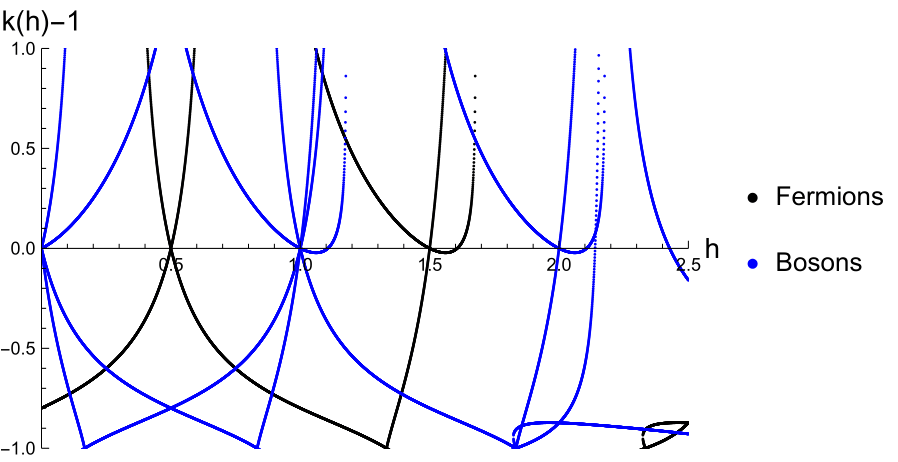
Figure 15: Case $p=q=3$, $\alpha=1$, $\mathcal{E}=\frac{1}{3}$. Shifted eigenvalues $k(h)-1$ of $K^{\mathrm{B}}$ (blue) and $K^{\mathrm{F}}$ (black) as the operator dimension $h$ varies. There is an operator $O_{h}$ in the spectrum whenever there is a horizontal intercept and $k(h)=1$. The total number of fermionic operators is doubled, due to the presence of $\overline{K}^{\mathrm{F}}$ as well.

Case $\boldsymbol{p=q=3}$.

For simplicity, we consider supersymmetric solutions with $\alpha=1$, so that there is a unique solution given in (3.39). We also fix $\mathcal{E}=\frac{1}{3}$ for definiteness. We read off the spectrum from Figure 15. Naively one would infer the presence of two $\mathcal{N}=2$ Schwarzian multiplets at $h=\bigl{(}1,2\times\frac{3}{2},2\bigr{)}$, however one of the two multiplets is spurious, due to an emergent IR reparametrization symmetry which is however incompatible with the UV boundary conditions [11, 26]. There appear also two $\mathcal{N}=2$ current multiplets at $h=\bigl{(}2\times\frac{1}{2},1\bigr{)}$, but one is again spurious for the same reason. Lastly, we notice the presence of a multiplet at $h\simeq\bigl{(}1.11,2\times 1.61,2.11\bigr{)}$. As pointed out in [7] and shown in [48, 49], the contribution of a bosonic operator $O_{h}$ with $1<h<\frac{3}{2}$ to the free energy is proportional to $\beta^{2-2h}$, which dominates over the $\beta^{-1}$ contribution from the Schwarzian at low temperatures. This implies that the IR physics in this solution should be non-universal and not described by the Schwarzian theory at leading order. We shall refer to the range $1<h<\frac{3}{2}$ as the “dangerous region”. Fermionic operators are excluded from this discussion since only bosonic operators can enter the Lagrangian as deformations.

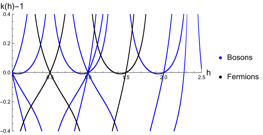
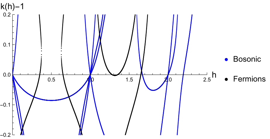
Figure 16: Case $p=1$, $q=2$, $\alpha=\frac{2}{3}$. Shifted eigenvalues $k(h)-1$ of $K^{\mathrm{B}}$ (blue) and $K^{\mathrm{F}}$ (black). Top: supersymmetric case with $\mathcal{E}_{\eta}=2\mathcal{E}$, $\mathcal{E}_{\phi}=-\mathcal{E}$, and $\mathcal{E}=0.05<\mathcal{E}_{*}\simeq 0.21$. Bottom: non-supersymmetric case with $\mathcal{E}_{\eta}=0.10$ and $\mathcal{E}_{\phi}=0.05$.

Case $\boldsymbol{p=1}$, $\boldsymbol{q=2}$.

In the supersymmetric case the unique solution is given in (3.33) and (3.34), which is valid for $0<\mathcal{E}<\mathcal{E}_{*}$. For concreteness, we fix $\alpha=\frac{2}{3}$ so that $\mathcal{E}_{*}\simeq 0.21$, and $\mathcal{E}=0.05$. Looking at the top of Figure 16, there appear two $\mathcal{N}=2$ Schwarzian multiplets at $h=\bigl{(}1,2\times\frac{3}{2},2\bigr{)}$ and two $\mathcal{N}=2$ current multiplets at $h=\bigl{(}2\times\frac{1}{2},1\bigr{)}$. Of these, only one Schwarzian multiplet and one current multiplet is physical while the other copy is spurious, as explained above. In addition, we notice a multiplet with $h\simeq\bigl{(}0.84,2\times 1.34,1.84\bigr{)}$. The presence of a bosonic operator $O_{h}$ with $h\simeq 0.84<1$ is not a cause for concern because this is a relevant deformation that can be tuned to zero by appropriately choosing the UV parameters. Therefore, we expect the IR physics of this solution to be dominated by the Schwarzian to leading order in $1/\beta$, and this is confirmed by the numerical results in Section 4.3. In the non-supersymmetric case we take $\mathcal{E}_{\eta}=0.1$ and $\mathcal{E}_{\phi}=0.05$ (they do not satisfy (3.27)) and the solution is obtained by solving (3.22) numerically. Looking at the bottom of Figure 16, we do not find a multiplet structure anymore. The presence of two Schwarzian modes ($h=2$) and four current modes ($h=1$) is still required by the symmetries of the theory — and half of these modes are spurious. We also discern two bosonic modes with $h\simeq 1.67,2.20$, outside the dangerous region. As expected, the fermionic modes split and move away from $h=\frac{1}{2},\frac{3}{2}$; there are in fact modes with $h\simeq 0.35,0.65,1.28,1.35,1.65$, all with multiplicity two.

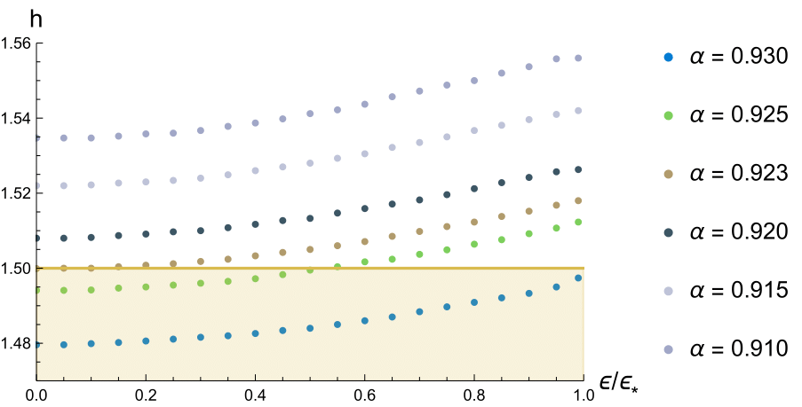
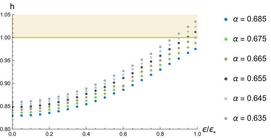
Figure 17: Case $p=1$, $q=2$. Bosonic operator dimensions closest to the dangerous region $1<h<\frac{3}{2}$, as $\alpha$ and $\mathcal{E}$ are varied. Different values of $\alpha$ are color coded. For $\alpha$ in the range $0.665\leq\alpha\leq 0.923$, no dangerous modes are present in the spectrum.

Since the Schwarzian mode can be the dominant one in the IR or not depending on the parameters $p,q,\alpha,\mathcal{E}$, we study in which ranges the two behaviours take place. As we will see, the spectrum is free of dangerous modes for $p=1$ and $0.665\leq\alpha\leq 0.923$, but not otherwise. It is reasonable to expect a qualitative difference between the models with $p=1$ and $p>1$, since the former has a scalar potential while the latter always contains fermions in its interaction terms.

In Figure 17 we consider the case $p=1$, $q=2$. We plot the dimensions of the bosonic operators which lie closest to the dangerous region $1<h<\frac{3}{2}$, as a function of $\mathcal{E}$. This is repeated for various values of $\alpha$. We observe that when the abundance parameter $\alpha$ is bigger than a critical value $\alpha_{\text{max}}\simeq 0.923$, dangerous modes appear at small values of $\mathcal{E}$. In this regime, we expect the IR physics not to be captured by the Schwarzian action, although we have not been able to observe this phenomenon numerically. Similarly, when $\alpha$ is smaller than a critical value $\alpha_{\text{min}}\simeq 0.665$, dangerous modes appear for large values of $\mathcal{E}$.

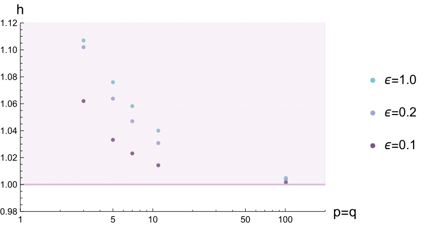
Figure 18: Cases with $p=q>1$ and $\alpha=1$. Bosonic operator dimensions in the dangerous region $1<h<\frac{3}{2}$ as $p=q$ are varied. Differently colored points correspond to different values of $\mathcal{E}$.

In Figure 18 we study the bosonic operators close to the dangerous region in the case $p=q>1$ and with $\alpha=1$. As $p=q$ is increased, one observes that the operator dimensions tend to $1$ from above, but are always within the dangerous region. This remains qualitatively unchanged for various values of $\mathcal{E}$, therefore we expect the IR physics not to be dominated by the Schwarzian mode for $p>1$.

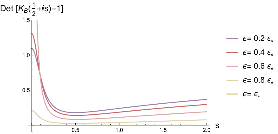
Figure 19: Plot of $\det(K^{\mathrm{B}}-\mathbbm{1})$ evaluated at $h=\frac{1}{2}+is$ against $s$. We fix $p=1$, $q=2$, $\alpha=2/3$ and vary $\mathcal{E}$ up to $\mathcal{E}_{*}$.

Since reality of the conformal Casimir $h(h-1)$ does not exclude complex values $h=\frac{1}{2}+is$ with $s\in\mathbb{R}$, the reality of the operator dimensions is a nontrivial consistency check of the spectrum. In Figure 19 we plot $\det(K^{\mathrm{B}}-\mathbbm{1})$ evaluated at $h=\frac{1}{2}+is$ against $s$ for $p=1$, $q=2$, $\alpha=\frac{2}{3}$ and various values of $\mathcal{E}$. An operator with complex dimension can exist only if $\det(K^{\mathrm{B}}-\mathbbm{1})=0$. For $\mathcal{E}<\mathcal{E}_{*}$ it is clear that $\det(K^{\mathrm{B}}-\mathbbm{1})$ is strictly positive and there are no such operators. As $\mathcal{E}\rightarrow\mathcal{E}_{*}$, the graph gets increasingly flatter and closer to the horizontal axis. This phenomenon was also present at a phase transition of the $\mathcal{N}=2$ model of [11], as discussed in [26].

6 Chaos exponents

An interesting feature to study both in quantum may-body systems and in toy models of quantum gravity is the quantum chaotic behaviour. From the gravity side, it has long been expected that black holes are maximally chaotic, see e.g. [50, 51, 52, 39], a feature that is captured by the standard SYK model [6]. In this section we compute the chaos exponents of various out-of-time-order correlators (OTOCs) in our models, using the retarded kernel approach of [13]. Working in components, we first introduce the various component 4-point functions and the integral equations that they satisfy, which follow from the superspace integral equation (5.13). We then define the OTOCs as analytic continuations of the 4-point functions and find the continued versions of the integral equations. Finally, analyzing the equations at late times, we determine the chaos exponents. It turns out that one of these exponents saturates the maximal chaos bound $\frac{2\pi}{\beta}$.

6.1 Integral equations for component 4-point functions

In components, eqn. (5.13) decomposes into 3 equalities: one for the $4\times 4$ matrix of bosonic 4-point functions:

$$F^{\mathrm{B}}(\tau_{1},\tau_{2};\tau_{3},\tau_{4})\equiv\lim_{N\to\infty}\Bigl{\langle}\delta G_{\bar{A}A}\,\delta G_{\bar{B}B}\Bigr{\rangle}_{4\times 4}(\tau_{1},\tau_{2};\tau_{3},\tau_{4})$$ (6.1)

with $A,B\in\{\eta,f,\phi,\psi\}$ and computed from the 2-point functions of bosonic bilocal fluctuations $\delta G_{\bar{A}A}$, and two for the $2\times 2$ matrices of fermionic 4-point functions:

$$F^{\mathrm{F}}\equiv\lim_{N\to\infty}\left\langle\begin{matrix}\delta G_{\bar{\eta}f}\delta G_{\bar{f}\eta}&\delta G_{\bar{\eta}f}\delta G_{\bar{\psi}\phi}\\ \delta G_{\bar{\phi}\psi}\delta G_{\bar{f}\eta}&\delta G_{\bar{\phi}\psi}\delta G_{\bar{\psi}\phi}\end{matrix}\right\rangle\;,\quad\overline{F}{}^{\mathrm{F}}\equiv\lim_{N\to\infty}\left\langle\begin{matrix}\delta G_{\bar{f}\eta}\delta G_{\bar{\eta}f}&\delta G_{\bar{f}\eta}\delta G_{\bar{\phi}\psi}\\ \delta G_{\bar{\psi}\phi}\delta G_{\bar{\eta}f}&\delta G_{\bar{\psi}\phi}\delta G_{\bar{\phi}\psi}\end{matrix}\right\rangle$$ (6.2)

computed from the 2-point functions of fermionic bilocal fluctuations $\delta G_{\bar{A}B}$. As in the previous section, this decomposition comes about because the kernel $\mathcal{K}$ does not mix bosonic and fermionic components. Specifically, (5.13) implies that $F^{\mathrm{B}}$, $F^{\mathrm{F}}$, $\overline{F}{}^{\mathrm{F}}$ satisfy the equations

$$F^{\mathrm{B}}(\tau_{1},\tau_{2};\tau_{3},\tau_{4}) =\frac{1}{1-K^{\mathrm{B}}}\cdot F^{\mathrm{B}}_{0}(\tau_{1},\tau_{2};\tau_{3},\tau_{4})=\sum\nolimits_{n=0}^{\infty}\bigl{(}K^{\mathrm{B}}\bigr{)}^{n}\cdot F_{0}^{\mathrm{B}}(\tau_{1},\tau_{2};\tau_{3},\tau_{4})\;,$$ (6.3)

$$F^{\mathrm{F}}(\tau_{1},\tau_{2};\tau_{3},\tau_{4}) =\frac{1}{1-K^{\mathrm{F}}}\cdot F_{0}^{\mathrm{F}}(\tau_{1},\tau_{2};\tau_{3},\tau_{4})=\sum\nolimits_{n=0}^{\infty}\bigl{(}K^{\mathrm{F}}\bigr{)}^{n}\cdot F_{0}^{\mathrm{F}}(\tau_{1},\tau_{2};\tau_{3},\tau_{4})\;,$$

$$\overline{F}{}^{\mathrm{F}}(\tau_{1},\tau_{2};\tau_{3},\tau_{4}) =\frac{1}{1-\overline{K}{}^{\mathrm{F}}}\cdot\bigl{(}F_{0}^{\mathrm{F}}\bigr{)}^{\sf{T}}(\tau_{1},\tau_{2};\tau_{3},\tau_{4})=\sum\nolimits_{n=0}^{\infty}\bigl{(}\overline{K}{}^{\mathrm{F}}\bigr{)}^{n}\cdot\bigl{(}F_{0}^{\mathrm{F}}\bigr{)}^{\sf{T}}(\tau_{1},\tau_{2};\tau_{3},\tau_{4})\;,$$

where $\cdot$ indicates the convolution $f\cdot g\,(\tau_{1},\tau_{2};\tau_{3},\tau_{4})=\int\!d\tau_{5}d\tau_{6}\,f(\tau_{1},\tau_{2};\tau_{5},\tau_{6})\,g(\tau_{5},\tau_{6};\tau_{3},\tau_{4})$ together with the standard matrix product, while ${\sf{T}}$ denotes both a matrix transpose and the swapping of arguments from $(\tau_{1},\tau_{2};\tau_{3},\tau_{4})$ to $(\tau_{3},\tau_{4};\tau_{1},\tau_{2})$. Lastly, $F_{0}^{\mathrm{B}}$ and $F_{0}^{\mathrm{F}}$ are the diagonal matrices

$$F_{0}^{\mathrm{B}}(\tau_{1},\tau_{2};\tau_{3},\tau_{4}) =\operatorname{diag}\Bigl{\{}-G_{\bar{\eta}\eta}^{*}(\tau_{1},\tau_{4})G_{\bar{\eta}\eta}^{*}(\tau_{3},\tau_{2})\,,G_{\bar{f}f}^{*}(\tau_{1},\tau_{4})G_{\bar{f}f}^{*}(\tau_{3},\tau_{2})\,,$$ (6.4)

$$\hskip 46.94687pt\tfrac{1}{\alpha}G_{\bar{\phi}\phi}^{*}(\tau_{1},\tau_{4})G_{\bar{\phi}\phi}^{*}(\tau_{3},\tau_{2})\,,-\tfrac{1}{\alpha}G_{\bar{\psi}\psi}^{*}(\tau_{1},\tau_{4})G_{\bar{\psi}\psi}^{*}(\tau_{3},\tau_{2})\Bigr{\}}\;,$$

$$F_{0}^{\mathrm{F}}(\tau_{1},\tau_{2};\tau_{3},\tau_{4}) =\operatorname{diag}\Bigl{\{}G^{*}_{\bar{f}f}(\tau_{3},\tau_{2})G^{*}_{\bar{\eta}\eta}(\tau_{1},\tau_{4})\,,-\tfrac{1}{\alpha}G_{\bar{\psi}\psi}^{*}(\tau_{3},\tau_{2})G_{\bar{\phi}\phi}^{*}(\tau_{1},\tau_{4})\Bigr{\}}\;.$$

Equivalently, (6.3) can be written as the integral equations

$$F(\tau_{1},\tau_{2};\tau_{3},\tau_{4})-\int\!d\tau_{5}\,d\tau_{6}\,K(\tau_{1},\tau_{2};\tau_{5},\tau_{6})\,F(\tau_{5},\tau_{6};\tau_{3},\tau_{4})=F_{0}(\tau_{1},\tau_{2};\tau_{3},\tau_{4})\;,$$ (6.5)

written in terms of $\{F^{\mathrm{B}},K^{\mathrm{B}},F_{0}^{\mathrm{B}}\}$, $\{F^{\mathrm{F}},K^{\mathrm{F}},F_{0}^{\mathrm{F}}\}$ and $\{\overline{F}{}^{\mathrm{F}},\overline{K}{}^{\mathrm{F}},(F_{0}^{\mathrm{F}})^{\sf{T}}\}$, respectively. Each component of these matrix equations is represented by a Feynman diagram of the form

(6.6)

In Appendix F, one can find the diagrams for each component of $K$ and $F_{0}$.

6.2 OTOCs and chaos exponents

The OTOCs we want to compute are double commutators such as

$$\frac{1}{N^{2}}\operatorname{Tr}\Bigl{(}\,e^{-\beta H}\,\Bigl{[}\,\overline{C}_{a}\bigl{(}\tfrac{\beta}{2}\bigr{)},B_{b}\bigl{(}\tfrac{\beta}{2}+it_{2}\bigr{)}\Bigr{]}\,\Bigl{[}\,\overline{A}_{b}(it_{1}),D_{a}(0)\,\Bigr{]}\,\Bigr{)}$$ (6.7)

$$=\frac{1}{N^{2}}\lim_{\epsilon\rightarrow 0^{+}}\Bigl{\langle}\Bigl{(}\overline{C}_{a}\bigl{(}\tfrac{\beta}{2}+\epsilon\bigr{)}-\overline{C}_{a}\bigl{(}\tfrac{\beta}{2}-\epsilon\bigr{)}\Bigr{)}\,B_{b}\bigl{(}\tfrac{\beta}{2}+it_{2}\bigr{)}\,\overline{A}_{b}(it_{1})\,\Bigl{(}D_{a}(-\epsilon)-D_{a}(\epsilon)\Bigr{)}\Bigr{\rangle}_{\beta}$$

$$=(-1)^{\xi_{1}[\bar{A},B,\bar{C}]}\lim_{\epsilon\rightarrow 0^{+}}\Bigl{\langle}G_{\bar{A}B}G_{\bar{C}D}\bigl{(}it_{1},\tfrac{\beta}{2}+it_{2};\tfrac{\beta}{2}+\epsilon,-\epsilon\bigr{)}-G_{\bar{A}B}G_{\bar{C}D}\bigl{(}it_{1},\tfrac{\beta}{2}+it_{2};\tfrac{\beta}{2}+\epsilon,\epsilon\bigr{)}$$

$$\hskip 96.73918pt+G_{\bar{A}B}G_{\bar{C}D}\bigl{(}it_{1},\tfrac{\beta}{2}+it_{2};\tfrac{\beta}{2}-\epsilon,\epsilon\bigr{)}-G_{\bar{A}B}G_{\bar{C}D}\bigl{(}it_{1},\tfrac{\beta}{2}+it_{2};\tfrac{\beta}{2}-\epsilon,-\epsilon\bigr{)}\Bigr{\rangle}\,.$$

Here $A$ is from the same multiplet as $B$, and $C$ is from the same multiplet as $D$, while the indices $a,b$ are summed over. If both $A$ and $D$ (or $B$ and $C$) are fermionic, the bracket $[\;,\,]$ between them should be understood as an anti-commutator. In the second line, the shifts of Euclidean time by $\pm\epsilon$ implement the operator ordering. We also defined the parity operator $\xi_{1}[\bar{A},B,\bar{C}]\equiv F[\bar{A}]\,F[B]+F[\bar{C}]\,F[\bar{A}B]$, where $F[\cdot]$ is the fermion number of a field, set to 0 for bosons and 1 for fermions. The OTOC is constructed so that it is computed by expectation values of bilocal fields in the third line, which are the only accessible observables after the disorder average. In addition, it is especially convenient to consider double commutators rather than a more general OTOC since we will see that the locations of operator insertions in the contributing diagrams are heavily constrained [13]. As seen from (5.12), such 4-point functions are computed at order $\mathcal{O}(1/N)$ by the expectation values $\langle\delta G_{\bar{A}B}\,\delta G_{\bar{C}D}\rangle$ of fluctuations around the conformal solutions, which are grouped into the matrices $F^{\mathrm{B}}$ and $F^{\mathrm{F}}$ in (6.1) and (6.2). The double commutators in (6.7) are therefore computed at this order by the following analytic continuations of $F^{\mathrm{B}}$ or $F^{\mathrm{F}}$:

$$W(t_{1},t_{2})\equiv\lim_{\epsilon\rightarrow 0^{+}}\Bigl{[}F\bigl{(}it_{1},\tfrac{\beta}{2}+it_{2};\tfrac{\beta}{2}+\epsilon,-\epsilon\bigr{)}-F\bigl{(}it_{1},\tfrac{\beta}{2}+it_{2};\tfrac{\beta}{2}+\epsilon,\epsilon\bigr{)}\\ {}+F\bigl{(}it_{1},\tfrac{\beta}{2}+it_{2};\tfrac{\beta}{2}-\epsilon,\epsilon\bigr{)}-F\bigl{(}it_{1},\tfrac{\beta}{2}+it_{2};\tfrac{\beta}{2}-\epsilon,-\epsilon\bigr{)}\Bigr{]}\,.$$ (6.8)

From here on, we will often omit the superscripts $\mathrm{B}$ and $\mathrm{F}$, since most of the steps are completely independent on them. We shall also consider another inequivalent double commutator where $\bar{A}$ and $B$ are swapped with respect to (6.7):

$$\frac{1}{N^{2}}\operatorname{Tr}\Bigl{(}e^{-\beta H}\,\Bigl{[}\overline{C}_{a}\bigl{(}\tfrac{\beta}{2}\bigr{)},\overline{A}_{b}\bigl{(}\tfrac{\beta}{2}+it_{1}\bigr{)}\Bigr{]}\,\Bigl{[}B_{b}(it_{2}),D_{a}(0)\Bigr{]}\Bigr{)}$$ (6.9)

$$=\frac{1}{N^{2}}\lim_{\epsilon\rightarrow 0^{+}}\Bigl{\langle}\Bigl{(}\overline{C}_{a}\bigl{(}\tfrac{\beta}{2}+\epsilon\bigr{)}-\overline{C}_{a}\bigl{(}\tfrac{\beta}{2}-\epsilon\bigr{)}\Bigr{)}\,\overline{A}_{b}\bigl{(}\tfrac{\beta}{2}+it_{1}\bigr{)}\,B_{b}(it_{2})\,\Bigl{(}D_{a}(-\epsilon)-D_{a}(\epsilon)\Bigr{)}\Bigr{\rangle}_{\beta}$$

$$=(-1)^{\xi_{2}[\bar{A},B,\bar{C}]}\lim_{\epsilon\rightarrow 0^{+}}\Bigl{\langle}G_{\bar{A}B}G_{\bar{C}D}\bigl{(}\tfrac{\beta}{2}+it_{1},it_{2};\tfrac{\beta}{2}+\epsilon,-\epsilon\bigr{)}-G_{\bar{A}B}G_{\bar{C}D}\bigl{(}\tfrac{\beta}{2}+it_{1},it_{2};\tfrac{\beta}{2}+\epsilon,\epsilon\bigr{)}$$

$$\hskip 93.89418pt+G_{\bar{A}B}G_{\bar{C}D}\bigl{(}\tfrac{\beta}{2}+it_{1},it_{2};\tfrac{\beta}{2}-\epsilon,\epsilon\bigr{)}-G_{\bar{A}B}G_{\bar{C}D}\bigl{(}\tfrac{\beta}{2}+it_{1},it_{2};\tfrac{\beta}{2}-\epsilon,-\epsilon\bigr{)}\Bigr{\rangle}\,,$$

where we defined $\xi_{2}[\bar{A},B,\bar{C}]\equiv F[\bar{C}]\,F[\bar{A}B]$. Analogously, it is computed at $\mathcal{O}(1/N)$ by different analytic continuations of $F^{\mathrm{B}}$ or $F^{\mathrm{F}}$:

$$\widetilde{W}(t_{1},t_{2})\equiv\lim_{\epsilon\rightarrow 0^{+}}\Bigl{[}F\bigl{(}\tfrac{\beta}{2}+it_{1},it_{2};\tfrac{\beta}{2}+\epsilon,-\epsilon\bigr{)}-F\bigl{(}\tfrac{\beta}{2}+it_{1},it_{2};\tfrac{\beta}{2}+\epsilon,\epsilon\bigr{)}\\ {}+F\bigl{(}\tfrac{\beta}{2}+it_{1},it_{2};\tfrac{\beta}{2}-\epsilon,\epsilon\bigr{)}-F\bigl{(}\tfrac{\beta}{2}+it_{1},it_{2};\tfrac{\beta}{2}-\epsilon,-\epsilon\bigr{)}\Bigr{]}\,.$$ (6.10)

According to one measure of quantum chaos, the order $\mathcal{O}(1/N)$ contributions to the double commutators of a chaotic theory at late times $t_{1}=t_{2}=t$ should behave as

$$W^{\mathrm{B},\mathrm{F}}(t,t)\,\propto\,\exp\bigl{[}\lambda_{L}^{\mathrm{B},\mathrm{F}}\,t\bigr{]}\;,$$ (6.11)

where $0<\lambda_{L}^{\mathrm{B},\mathrm{F}}\leq\frac{2\pi}{\beta}$ are the so-called Lyapunov exponents [13]. The goal in the following is to compute these exponents using the retarded kernel approach.

6.3 The retarded kernel

The strategy in the retarded-kernel approach is to use analytically continued versions of (6.5) to constrain $W$ and $\widetilde{W}$. Looking at the definitions (6.8) and (6.10), it is apparent that one should sum four copies of (6.5) with $\tau_{3}$ and $\tau_{4}$ appropriately shifted by $\pm\epsilon$. We first consider $\tau_{1}=it_{1}$ and $\tau_{2}=\frac{\beta}{2}+it_{2}$, so that $W$ is obtained from the first term of (6.5):

$$W(t_{1},t_{2})-\lim_{\epsilon\rightarrow 0^{+}}\int\!d\tau_{3}\,d\tau_{4}\;K\bigl{(}it_{1},\tfrac{\beta}{2}+it_{2};\tau_{3},\tau_{4}\bigr{)}\Bigl{[}F\bigl{(}\tau_{3},\tau_{4};\tfrac{\beta}{2}+\epsilon,-\epsilon\bigr{)}$$ (6.12)

$$\hskip 56.9055pt-F\bigl{(}\tau_{3},\tau_{4};\tfrac{\beta}{2}+\epsilon,\epsilon\bigr{)}+F\bigl{(}\tau_{3},\tau_{4};\tfrac{\beta}{2}-\epsilon,\epsilon\bigr{)}-F\bigl{(}\tau_{3},\tau_{4};\tfrac{\beta}{2}-\epsilon,-\epsilon\bigr{)}\Bigr{]}=W_{0}(t_{1},t_{2})\;,$$

where $W_{0}(t_{1},t_{2})$ is defined as in (6.8) but using $F_{0}$ in place of $F$. We should determine the integration contour for $\tau_{3},\tau_{4}$ in the second term of (6.5), and it is useful to note that $\tau_{3},\tau_{4}$ are the locations of interaction vertices in the Feynman diagrams drawn in (6.6). In the path integral, Feynman vertices are derived from local interaction terms in the action, which have the form $\int\!d\tau\,O(\tau)$. Integrals over the positions of the vertices come directly from the time integral in the action, therefore specifying the complex time contour that is used to compute the path integral also specifies the contour for the vertex positions. Since we are computing the double commutator (6.7), the contour must pass through all operator insertions in the double commutator. We shall choose the same contour as in [13], shown in Figure 20. The folds that pass through $\tau_{1}$ and $\tau_{2}$ are called the left and right rails; each rail has a left and a right side. The four contributing terms in (6.8) correspond to different positions for the operator insertions at the bottom of the rails.

Figure 20: Contour in the complex $\tau$ plane used for the evaluation of (6.5) and (6.7). The four terms in the double commutator correspond to the choices of placing an operator at $\pm\epsilon$, and another one at $\frac{\beta}{2}\pm\epsilon$.

A priori the interaction vertices at $\tau_{3}$ and $\tau_{4}$ could be placed at any point on the contour in Figure 20, and the integrals should be performed over the whole contour. However, it turns out that nonzero contributions to the integrals only occur when there is one vertex on each rail. This is because if the left rail is free of vertices, the 4-point functions computed by $F\bigl{(}\tau_{3},\tau_{4};\frac{\beta}{2}+\epsilon,\pm\epsilon\bigr{)}$ are equal as $\epsilon\rightarrow 0$, since there is no difference in operator ordering. Consequently, the four terms under the integral in (6.12) cancel. Similarly, if the right rail is free of vertices, the 4-point functions computed by $F\bigl{(}\tau_{3},\tau_{4};\frac{\beta}{2}\pm\epsilon,\epsilon\bigr{)}$ are equal and the same cancellation occurs. Moreover, $\tau_{3}$ must be on the right rail and $\tau_{4}$ on the left rail, but not the other way around. To see this, we first note from (E.5) that the time dependence in every component of the kernels $K^{\mathrm{B},\mathrm{F}}$ is given by a product of 3 conformal 2-point functions:

$$K_{\bar{A}B,\bar{C}D}(\tau_{1},\tau_{2};\tau_{3},\tau_{4})\;\propto\;G^{\beta}_{s_{1}}(\tau_{14};\Delta_{1},\mathcal{E}_{1})\,G^{\beta}_{s_{2}}(\tau_{32};\Delta_{2},\mathcal{E}_{2})\,G^{\beta}_{s_{3}}(\tau_{34};\Delta_{3},\mathcal{E}_{3})\;.$$ (6.13)

Suppose instead that $\tau_{3}$ is on the left rail. Then $\tau_{3}=\pm\tilde{\epsilon}+it_{3}$ for some $\tilde{\epsilon}\in(0,\epsilon)$, where the plus/minus sign corresponds to $\tau_{3}$ being on the right/left side of the rail, respectively. Since $G^{\beta}_{s_{2}}(\tau_{32};\Delta_{2},\mathcal{E}_{2})=G_{s_{2}}^{\beta}(-\frac{\beta}{2}\pm\epsilon+it_{32};\Delta_{2},\mathcal{E}_{2})$ has a smooth limit as $\epsilon\rightarrow 0$, the integrand in (6.12) is equal for the two sides of the rail. However, the contour in Figure 20 runs from left to right with increasing $\operatorname{\mathbb{R}e}\tau$, and there is a relative sign in the integration measure $d\tau_{3}=\pm i\,dt_{3}$ between the sides of the rail. Hence the contributions from the two sides cancel.

On the remaining contour where contributions are nonzero, $\tau_{3}=\frac{\beta}{2}+s_{4}\,\tilde{\epsilon}+it_{3}$ and $\tau_{4}=s_{5}\,\tilde{\epsilon}+it_{4}$ with $\tilde{\epsilon}\in(0,\epsilon)$. The signs $s_{4,5}=\pm 1$ parametrize whether $\tau_{3,4}$ are on the right or left side of the rails, and they should be summed over. Recall that the contour orientation depends on which side we are on, so $d\tau_{3,4}=-i\,s_{4,5}\,dt_{3,4}$. Substituting this contour and (6.13) into the integral term of (6.12), every component is a sum of terms proportional to

$$\lim_{\epsilon\rightarrow 0^{+}}\sum_{s_{4},s_{5}=\pm 1}(-s_{4}s_{5})\int_{0}^{t_{2}}\!dt_{3}\int_{0}^{t_{1}}\!dt_{4}\;G_{1}^{\beta}\bigl{(}-s_{5}\tilde{\epsilon}+it_{14}\bigr{)}\,G_{2}^{\beta}\bigl{(}s_{4}\tilde{\epsilon}+it_{32}\bigr{)}\,G_{3}^{\beta}\bigl{(}\tfrac{\beta}{2}+it_{34}\bigr{)}\times{}$$ (6.14)

$$\times\Bigl{[}F_{\bar{C}D}\bigl{(}\tfrac{\beta}{2}+s_{4}\tilde{\epsilon}+it_{3},s_{5}\tilde{\epsilon}+it_{4};\tfrac{\beta}{2}+\epsilon,-\epsilon\bigr{)}-F_{\bar{C}D}\bigl{(}\tfrac{\beta}{2}+s_{4}\tilde{\epsilon}+it_{3},s_{5}\tilde{\epsilon}+it_{4};\tfrac{\beta}{2}+\epsilon,\epsilon\bigr{)}$$

$$\quad+F_{\bar{C}D}\bigl{(}\tfrac{\beta}{2}+s_{4}\tilde{\epsilon}+it_{3},s_{5}\tilde{\epsilon}+it_{4};\tfrac{\beta}{2}-\epsilon,\epsilon\bigr{)}-F_{\bar{C}D}\bigl{(}\tfrac{\beta}{2}+s_{4}\tilde{\epsilon}+it_{3},s_{5}\tilde{\epsilon}+it_{4};\tfrac{\beta}{2}-\epsilon,-\epsilon\bigr{)}\Bigr{]}\;,$$

where $F_{\bar{C}D}$ is a component of $F$, and appropriate dependencies on the conformal ansatz parameters are implied for $G^{\beta}$. Since $\tilde{\epsilon}\in(0,\epsilon)$, $\operatorname{sign}(\pm\epsilon-s_{4,5}\tilde{\epsilon})=\pm 1$ and the operator ordering in the four $F_{\bar{C}D}$ is unaffected if we send $\tilde{\epsilon}\rightarrow 0$ at fixed $\epsilon$. This simplifies (6.14) to

$$\int_{0}^{t_{2}}\!dt_{3}\int_{0}^{t_{1}}\!dt_{4}\;G^{\mathrm{R}}_{s_{1}}(t_{14};\Delta_{1},\mathcal{E}_{1})\;\overline{G^{\mathrm{R}}_{s_{2}}(t_{23};\Delta_{2},\mathcal{E}_{2})}\;G^{\text{lr}}_{s_{3}}(t_{34};\Delta_{3},\mathcal{E}_{3})\;\widetilde{W}_{\bar{C}D}(t_{3},t_{4})\;,$$ (6.15)

where we defined

$$G_{s}^{\mathrm{R}}(t;\Delta,\mathcal{E}) \equiv\lim_{\epsilon\rightarrow 0^{+}}\sum_{s^{\prime}=\pm 1}s^{\prime}G_{s}^{\beta}(s^{\prime}\epsilon+it;\Delta,\mathcal{E})=\,\frac{2\pi^{2\Delta}e^{-i\pi\frac{1+s}{4}-\frac{2\pi i\mathcal{E}}{\beta}t}}{\Bigl{[}\beta\sinh\bigl{(}\frac{\pi t}{\beta}\bigr{)}\Bigr{]}^{2\Delta}}\,\sin\Bigl{(}\pi\bigl{(}\Delta+\tfrac{1-s}{4}+i\mathcal{E}\bigr{)}\Bigr{)}\,,$$

$$G^{\text{lr}}(t;\Delta,\mathcal{E}) \equiv G_{s}^{\beta}\bigl{(}\tfrac{\beta}{2}+it;\Delta,\mathcal{E}\bigr{)}=\frac{\pi^{2\Delta}\,e^{-\frac{2\pi i\mathcal{E}}{\beta}t}}{\Bigl{[}\beta\cosh\bigl{(}\frac{\pi t}{\beta}\bigr{)}\Bigr{]}^{2\Delta}}\,.$$ (6.16)

Note that $G^{\mathrm{R}}_{s}(-t;\Delta,\mathcal{E})=\overline{G^{\mathrm{R}}_{s}(t;\Delta,\mathcal{E})}$. In the literature, $G^{\mathrm{R}}_{s}$ is sometimes called the retarded propagator while $G^{\text{lr}}$ is called the ladder-rung propagator, due to how they arise from propagators connecting the interaction vertices, which run horizontally between the vertical rails in Figure 20.

Therefore, we have shown that (6.12) can be written as

$$W(t_{1},t_{2})-\int_{0}^{t_{2}}\!dt_{3}\int_{0}^{t_{1}}\!dt_{4}\;K_{\mathrm{R}}^{+}(t_{1},t_{2};t_{3},t_{4})\;\widetilde{W}(t_{3},t_{4})=W_{0}(t_{1},t_{2})\;,$$ (6.17)

where the components of $K_{\mathrm{R}}^{+}$ are obtained from those of $K$ through the replacements $G^{\beta}_{1}(\tau_{14})\,G^{\beta}_{2}(\tau_{32})\,G^{\beta}_{3}(\tau_{34})\rightarrow G^{\mathrm{R}}_{1}(t_{14})\,\overline{G^{\mathrm{R}}_{2}(t_{23})}\,G^{\text{lr}}_{3}(t_{34})$. On the other hand, one could choose $\tau_{1}=\frac{\beta}{2}+it_{1}$, $\tau_{2}=it_{2}$ and sum over four copies of (6.5) to construct an analog of (6.12) in which the first term is $\widetilde{W}(t_{1},t_{2})$. Following the same steps as the above, one obtains an equation as (6.17) but in which $W\leftrightarrow\widetilde{W}$, $K_{\mathrm{R}}^{+}\to K_{\mathrm{R}}^{-}$ and $W_{0}\to\widetilde{W}_{0}$, where

$$\widetilde{W}_{0}(t_{1},t_{2})\equiv\lim_{\epsilon\rightarrow 0^{+}}\Bigl{[}F_{0}\bigl{(}\tfrac{\beta}{2}+it_{1},it_{2};\tfrac{\beta}{2}+\epsilon,-\epsilon\bigr{)}-F_{0}\bigl{(}\tfrac{\beta}{2}+it_{1},it_{2};\tfrac{\beta}{2}+\epsilon,\epsilon\bigr{)}\\ {}+F_{0}\bigl{(}\tfrac{\beta}{2}+it_{1},it_{2};\tfrac{\beta}{2}-\epsilon,\epsilon\bigr{)}-F_{0}\bigl{(}\tfrac{\beta}{2}+it_{1},it_{2};\tfrac{\beta}{2}-\epsilon,-\epsilon\bigr{)}\Bigr{]}$$ (6.18)

while the components of $K_{\mathrm{R}}^{-}$ are obtained from those of $K$ via $G^{\beta}_{1}(\tau_{14})\,G^{\beta}_{2}(\tau_{32})\,G^{\beta}_{3}(\tau_{34})\rightarrow s_{3}\,G^{\mathrm{R}}_{1}(t_{14})\,\overline{G^{\mathrm{R}}_{2}(t_{23})}\,G^{\text{lr}}(t_{34})$. Note that the only difference between the replacements to use in $K_{\mathrm{R}}^{+}$ and $K_{\mathrm{R}}^{-}$ is the sign $s_{3}$. Due to the mixing between $W$ and $\widetilde{W}$, it is convenient to group (6.17) and its analog for $\widetilde{W}$ into a single equation:

$$\bigg{(}\begin{matrix}W\\ \widetilde{W}\end{matrix}\biggr{)}(t_{1},t_{2})-\int_{0}^{t_{2}}\!dt_{3}\int_{0}^{t_{1}}\!dt_{4}\;K_{R}(t_{1},t_{2};t_{3},t_{4})\;\biggl{(}\begin{matrix}W\\ \widetilde{W}\end{matrix}\biggr{)}(t_{3},t_{4})=\biggl{(}\begin{matrix}W_{0}\\ \widetilde{W}_{0}\end{matrix}\biggr{)}(t_{1},t_{2})$$ (6.19)

where we introduced the matrix $K_{\mathrm{R}}=\Bigl{(}\begin{smallmatrix}0&K_{\mathrm{R}}^{+}\\ K_{\mathrm{R}}^{-}&0\end{smallmatrix}\Bigr{)}$. Assuming that $W$ and $\widetilde{W}$ are exponentially increasing at late times, the right hand side of (6.19) is in comparison exponentially suppressed and can be neglected. Furthermore, the lower limits of integration can be modified to $-\infty$ at this order of approximation, since the dominant contribution to the integral comes from $t_{3,4}$ close to $t_{1,2}$ [13]. The equation we are left with shows that if $W$ and $\widetilde{W}$ are chaotic, their columns are eigenvectors of the retarded kernel $K_{\mathrm{R}}$ with eigenvalue $1$. We find it convenient to change variables to

$$z_{1,4}=e^{-\frac{2\pi t_{1,4}}{\beta}}\,,\quad z_{2,3}=-e^{-\frac{2\pi t_{2,3}}{\beta}}\,,\quad\int_{-\infty}^{t_{2}}\!dt_{3}\int_{-\infty}^{t_{1}}\!dt_{4}=\int_{-\infty}^{z_{2}}\!dz_{3}\int_{z_{1}}^{\infty}\!dz_{4}\,\frac{(\beta/2\pi)^{2}}{|z_{3}||z_{4}|}\,,$$ (6.20)

after which the eigenvalue equation becomes

$$\biggl{(}\begin{matrix}W\\ \widetilde{W}\end{matrix}\biggr{)}(z_{1},z_{2})=\int_{-\infty}^{z_{2}}\!dz_{3}\int_{z_{1}}^{\infty}\!dz_{4}\;K_{\mathrm{R}}(z_{1},z_{2};z_{3},z_{4})\;\biggl{(}\begin{matrix}W\\ \widetilde{W}\end{matrix}\biggr{)}(z_{3},z_{4})\;.$$ (6.21)

Notice that, with some abuse of notation, here we defined

$$|z_{3}z_{4}|\;K_{\mathrm{R}}(z_{1},z_{2};z_{3},z_{4})=\bigl{(}\tfrac{\beta}{2\pi}\bigr{)}^{2}\;K_{\mathrm{R}}\bigl{(}t(z_{1}),t(z_{2});t(z_{3}),t(z_{4})\bigr{)}\;.$$ (6.22)

6.4 Exponents from the fermionic and bosonic retarded kernels

Applying the replacements that lead to $K_{\mathrm{R}}^{\pm}$ to (E.3) and (E.1), we obtain the retarded kernel $K_{\mathrm{R}}$ in the $t$ coordinates, appearing in (6.19), whose components are listed in (E.14) and (E.13). After performing the change of variables (6.20), the components of $K_{\mathrm{R}}$ in the $z$ coordinates are obtained through the substitution (E.16). The goal is now to find eigenvectors of $K_{\mathrm{R}}^{\mathrm{B}}$ and $K_{\mathrm{R}}^{\mathrm{F}}$ with eigenvalue $1$, which form the columns of $\bigl{(}W^{\mathrm{B}},\widetilde{W}^{\mathrm{B}}\bigr{)}{}^{\sf{T}}$ and $\bigl{(}W^{\mathrm{F}},\widetilde{W}^{\mathrm{F}}\bigr{)}{}^{\sf{T}}$, and extract their exponents at late times.

Each component $K_{\bar{A}B,\bar{C}D}^{\mathrm{R}}(z_{1},z_{2};z_{3},z_{4})$ has the form

$$K_{\bar{A}B,\bar{C}D}^{\mathrm{R}}=\frac{g_{L(A)}\bigl{(}\frac{2\pi}{\beta}\bigr{)}^{\Delta_{A}+\Delta_{B}}|z_{1}|^{\Delta_{A}+i\mathcal{E}_{A}}|z_{2}|^{\Delta_{B}-i\mathcal{E}_{B}}}{g_{L(C)}\bigl{(}\frac{2\pi}{\beta}\bigr{)}^{\Delta_{C}+\Delta_{D}}|z_{3}|^{\Delta_{C}+i\mathcal{E}_{C}}|z_{4}|^{\Delta_{D}-i\mathcal{E}_{D}}}\times\frac{K}{|z_{14}|^{2\Delta_{A}}|z_{23}|^{2\Delta_{B}}|z_{34}|^{2-\Delta_{A}-\Delta_{B}-\Delta_{C}-\Delta_{D}}}\,,$$

where $K$ is some $z$-independent proportionality constant that does not depend on the coefficients $g_{\eta,\phi}$. Note that the components $K_{\bar{A}B,\bar{C}D}^{\mathrm{R}}$ are labelled such that $\bar{A}B$ is a row index and $\bar{C}D$ is a column index in the matrices $K^{\mathrm{B},\pm}_{\mathrm{R}}$, $K^{\mathrm{F},\pm}_{\mathrm{R}}$. In a column of $\bigl{(}W^{\mathrm{B}},\widetilde{W}^{\mathrm{B}}\bigr{)}{}^{\sf{T}}$ or $\bigl{(}W^{\mathrm{F}},\widetilde{W}^{\mathrm{F}}\bigr{)}{}^{\sf{T}}$ on which $K^{\mathrm{B},\pm}_{\mathrm{R}}$ and $K^{\mathrm{F},\pm}_{\mathrm{R}}$ act respectively, we naturally label the component that is being contracted with $K_{\bar{A}B,\bar{C}D}^{\mathrm{R}}$ as $W_{\bar{C}D}$ or $\widetilde{W}_{\bar{C}D}$. It is then straightforward to check that the eigenfunctions of $K_{\bar{A}B,\bar{C}D}^{\mathrm{R}}$ under convolution are

$$w_{\bar{C}D}(z_{3},z_{4})\,\equiv\,g_{L(C)}\,\biggl{(}\frac{2\pi}{\beta}\biggr{)}^{\Delta_{C}+\Delta_{D}}\,\frac{|z_{3}|^{\Delta_{C}+i\mathcal{E}_{C}}\,|z_{4}|^{\Delta_{D}-i\mathcal{E}_{D}}}{|z_{34}|^{\Delta_{C}+\Delta_{D}-h}}\;,$$ (6.23)

where $h$ is a free parameter that will be determined below by requiring that (6.21) be satisfied. Indeed we have:

$$\int_{-\infty}^{z_{2}}\!dz_{3}\int_{z_{1}}^{\infty}\!dz_{4}\;K_{\bar{A}B,\bar{C}D}^{\mathrm{R}}(z_{1},z_{2};z_{3},z_{4})\;w_{\bar{C}D}(z_{3},z_{4})={}$$ (6.24)

$$\;\;=K\,g_{L(A)}\biggl{(}\frac{2\pi}{\beta}\biggr{)}^{\!\Delta_{A}+\Delta_{B}}\!|z_{1}|^{\Delta_{A}+i\mathcal{E}_{A}}|z_{2}|^{\Delta_{B}-i\mathcal{E}_{B}}\int_{-\infty}^{z_{2}}\!\!dz_{3}\!\int_{z_{1}}^{\infty}\!\!\!dz_{4}\;\frac{1}{|z_{14}|^{2\Delta_{A}}|z_{23}|^{2\Delta_{B}}|z_{34}|^{2-\Delta_{A}-\Delta_{B}-h}}$$

$$\;\;=K\;\frac{\Gamma(1-2\Delta_{A})\,\Gamma(1-2\Delta_{B})\,\Gamma(\Delta_{A}+\Delta_{B}-h)}{\Gamma(2-\Delta_{A}-\Delta_{B}-h)}\;w_{\bar{A}B}(z_{1},z_{2})\;.$$

We therefore take $W_{\bar{A}B}(z_{1},z_{2})$ to be proportional to $w_{\bar{A}B}(z_{1},z_{2})$. At $t_{1}=t_{2}=t$, the time dependence in $w_{\bar{A}B}$ is

$$w_{\bar{A}B}\Bigl{(}e^{-\frac{2\pi t}{\beta}},-e^{-\frac{2\pi t}{\beta}}\Bigr{)}\,\propto\,\exp\biggl{[}\frac{2\pi t}{\beta}\,(-h+i\mathcal{E}_{B}-i\mathcal{E}_{A})\biggr{]}\;.$$ (6.25)

The Lyapunov exponent is thus given by $\lambda=-\frac{2\pi}{\beta}\operatorname{\mathbb{R}e}h$ for values of $h$ such that $K_{\mathrm{R}}$ has eigenvalue $1$. In particular, we must have $-1\leq\operatorname{\mathbb{R}e}h<0$ for consistency with the assumption of exponential growth that was used to simplify the computation previously, and with the maximal chaos bound $\lambda\leq\frac{2\pi}{\beta}$.

When acting on (6.24), $K_{\mathrm{R}}$ is represented by an ordinary matrix. The bosonic retarded kernel $K^{\mathrm{B}}_{\mathrm{R}}$ and the fermionic retarded kernel $K^{\mathrm{F}}_{\mathrm{R}}$ can be found in (E.17) and (E.18), respectively. We compute the chaos exponents by finding values of $h$ at which $\det\big{(}K_{\mathrm{R}}^{\mathrm{B},\mathrm{F}}-\mathbbm{1}\bigr{)}=0$. Remarkably, $\det\bigl{[}K_{\mathrm{R}}^{\mathrm{F}}(h=-1/2)-\mathbbm{1}_{4\times 4}\bigr{]}=\det\bigl{[}K_{\mathrm{R}}^{\mathrm{B}}(h=-1)-\mathbbm{1}_{8\times 8}\bigr{]}=0$ holds regardless of the dimensions $\Delta_{\eta,\phi}$, as long as they satisfy the supersymmetry constraint $p\Delta_{\eta}+q\Delta_{\phi}=\frac{1}{2}$. This shows that on all superconformal solutions, there is maximal and half-maximal chaos in the double commutators computed by $\bigl{(}W^{\mathrm{B}},\widetilde{W}^{\mathrm{B}}\bigr{)}$ and $\bigl{(}W^{\mathrm{F}},\widetilde{W}^{\mathrm{F}}\bigr{)}$, respectively.

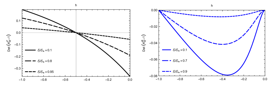
Figure 21: Plots of $\det\bigl{(}K_{\mathrm{R}}^{\mathrm{F}}-\mathbbm{1}_{4\times 4}\bigr{)}$ in black (left) and $\det\bigl{(}K_{\mathrm{R}}^{\mathrm{B}}-\mathbbm{1}_{8\times 8}\bigr{)}$ in blue (right) against $h$, for the solution (3.33) at $\alpha=\frac{1}{2}$ and various values of $\mathcal{E}$ as a fraction of the critical value $\mathcal{E}_{*}=\frac{1}{\pi}\operatorname{arctanh}\bigl{(}1/\sqrt{2}\bigr{)}$.

In addition, for the analytic superconformal solutions found in Section 3.4 there are no other values of $h\in[-1,0)$ at which $\det\bigl{(}K_{\mathrm{R}}^{\mathrm{B},\mathrm{F}}-\mathbbm{1}\bigr{)}=0$. For example, in Figure 21 we plot $\det\bigl{(}K_{\mathrm{R}}^{\mathrm{F}}-\mathbbm{1}_{4\times 4}\bigr{)}$ in black on the left and $\det\bigl{(}K_{\mathrm{R}}^{\mathrm{B}}-\mathbbm{1}_{8\times 8}\bigr{)}$ in blue on the right against $h$, for the solution (3.33) and various values of $\mathcal{E}$. It is clear that there are no other zeros except at $h=-\frac{1}{2},-1$. The same qualitative behaviour is found for other superconformal solutions. This suggests that for superconformal solutions there are no other chaos exponents except the maximal and half-maximal ones that we found.

7 Discussion

For $p=1$, our model bears many similarities with that of [28], although the abundance parameter and the coupling of the fermions make it irredeemably distinct. In the conformal phase of our model, the low-energy behaviour is closer to standard SYK and thus avoids completely the “curious” behaviour of the model in [28]. Naively, even outside of the conformal phase the models behave differently, with the dynamical bosonic correlator taking an exponential-like profile instead of a constant. However, it is possible that it realizes a charged version of the phase identified in [28]. This is consistent with $\Delta_{\phi}\rightarrow 0$ at the transition point, and numerically we do not rule out a sub-Schwarzian mode which scales with $T^{\gamma}$ for non-integer $\gamma$. However, further study would be required to check whether there is a meaningful connection.

Another interesting aspect of this model which could benefit from analytical understanding is the “emergent” supersymmetric behaviour discussed in Section 4. It would be interesting, for example, to derive the relation (4.5) analytically. A perhaps more crucial question is to ascertain whether this is a physical phenomenon or simply an artifact of the Schwinger–Dyson equations. It is not clear, for example, if one can reconcile such an IR behaviour and the arguments in Appendix C.2 which set $2\pi\mathcal{E}=-\beta\mu$ by combining Ward identities and (anti-)periodicity. Could the chemical potentials be “renormalized” in the IR? Or should one consider these solutions to be simply outside of the physical Hilbert space? An actual implementation of the model could clear this up, as could some holographic argument.

The dependency of the Schwarzian coupling on the charge $\mathcal{Q}$ is another point for which we found numerical results but with insufficient precision to be conclusive. Far from the critical value of $\mu$, the variation of the coupling with the charge seems to be very flat but probably not constant. This contrasts with some known black hole setups such as [53] where the coupling varies with a rational power of the charge. Perhaps a specific gravitational dual to this model could enlighten this aspect, since in SYK-like models the Schwarzian coupling is notoriously difficult to fix from the quantum mechanical side alone. Another aspect on which the numerical analysis is not conclusive and would benefit from analytic control is whether a phase transition truly happens at the critical chemical potential.

This leads to a final interesting challenge, which is whether there is a concrete and specific gravity dual to this model. In particular, both the inspiration from the quantum mechanical model of [29] and the phases of solutions described in Section 3.4 suggest that the case $p=1$, $q=2$ is the most “black-hole-like”, which is also the case in which we found most of the interesting numerical results.

It would also be interesting to study the finite $N$ model numerically, before taking the approximation of the Schwinger–Dyson equation. This would require us to truncate the bosonic Hamiltonian, or to consider a version with spin or hard bosons. This could confirm the absence of a spin-glass phase.

Appendix A Superspace conventions

In this appendix we collect our conventions about superspace and super-reparametrizations. In terms of superspace coordinates, the supercharges are

$$Q=\partial_{\theta}-\frac{\overline{\theta}}{2}\,\partial_{\tau}\;,\qquad\qquad\overline{Q}=-\partial_{\overline{\theta}}+\frac{\theta}{2}\,\partial_{\tau}\;,$$ (A.1)

with $Q^{2}=\overline{Q}{}^{2}=0$ and $\{Q,\overline{Q}\}=\partial_{\tau}$. The chiral and anti-chiral superspace derivatives are

$$D=\partial_{\theta}+\frac{\overline{\theta}}{2}\,\partial_{\tau}\;,\qquad\overline{D}=-\partial_{\overline{\theta}}-\frac{\theta}{2}\,\partial_{\tau}\;,\qquad\{D,\overline{D}\}=-\partial_{\tau}\;.$$ (A.2)

They satisfy $\{D,Q\}=\{D,\overline{Q}\}=\{\overline{D},Q\}=\{\overline{D},\overline{Q}\}=0$. Chiral superfields $\Phi$ and Fermi superfields $\mathcal{Y}$ (and they anti-chiral counterparts) have expansions

$$\Phi =\phi+\theta\psi+\frac{1}{2}\theta\overline{\theta}\,\partial_{\tau}\phi\;,\qquad \overline{\Phi} =\overline{\phi}-\overline{\theta}\,\overline{\psi}-\frac{1}{2}\theta\overline{\theta}\,\partial_{\tau}\overline{\phi}\;,$$ (A.3)

$$\mathcal{Y} =\eta-\theta f+\frac{1}{2}\theta\overline{\theta}\,\partial_{\tau}\eta\;,\qquad \overline{\mathcal{Y}} =\overline{\eta}-\overline{\theta}\,\overline{f}-\frac{1}{2}\theta\overline{\theta}\,\partial_{\tau}\overline{\eta}\;.$$

They satisfy $\overline{D}\Phi=D\overline{\Phi}=\overline{D}\mathcal{Y}=D\overline{\mathcal{Y}}=0$. In our conventions, conjugation reverses the order of fermions. The integration measure over full superspace is written as $d^{3}T\equiv d\tau d\theta d\overline{\theta}$, while the measures over chiral and anti-chiral superspaces are $d^{2}T\equiv d\tau d\theta$ and $d^{2}\overline{T}\equiv d\tau d\overline{\theta}$, respectively. The measures over half superspace are fermionic: they anti-commute among themselves and with other fermionic operators like $D$, $\overline{D}$. The superspace delta functions

$$\delta^{3}(T_{1}-T_{2}) \equiv(\overline{\theta}_{1}-\overline{\theta}_{2})\,(\theta_{1}-\theta_{2})\,\delta(\tau_{1}-\tau_{2})\;,$$ (A.4)

$$\delta^{2}(T_{1},T_{2}) \equiv\overline{D}_{2}\,\delta^{3}(T_{1}-T_{2})=(\theta_{1}-\theta_{2})\,\delta\Bigl{(}\tau_{1}-\tau_{2}+\tfrac{1}{2}\theta_{1}\overline{\theta}_{1}-\tfrac{1}{2}\theta_{2}\overline{\theta}_{2}\Bigr{)}\;,$$

$$\overline{\delta}{}^{2}(T_{1},T_{2}) \equiv D_{2}\,\delta^{3}(T_{1}-T_{2})=(\overline{\theta}_{1}-\overline{\theta}_{2})\,\delta\Bigl{(}\tau_{1}-\tau_{2}-\tfrac{1}{2}\theta_{1}\overline{\theta}_{1}+\tfrac{1}{2}\theta_{2}\overline{\theta}_{2}\Bigr{)}\;,$$

are defined to satisfy

$$\int\!d^{3}T_{1}\;\delta^{3}(T_{1}-T_{2})\,X(T_{1}) =X(T_{2})\;,\qquad \text{for $X$ generic}\;,$$ (A.5)

$$\int\!d^{2}T_{1}\;\delta^{2}(T_{1}-T_{2})\,\Phi(T_{1}) =\Phi(T_{2})\;,\qquad \text{for }\overline{D}\Phi=0\;,$$

$$\int\!d^{2}\overline{T}_{1}\;\overline{\delta}{}^{2}(T_{1}-T_{2})\,\overline{\Phi}(T_{1}) =\overline{\Phi}(T_{2})\;,\qquad \text{for }D\overline{\Phi}=0\;.$$

Note that $\delta^{2}$ is chiral in both arguments, and $\overline{\delta}{}^{2}$ is anti-chiral in both arguments. Besides, $\delta^{3}$ is bosonic and even in the two arguments, whilst $\delta^{2}$ and $\overline{\delta}{}^{2}$ are fermionic and anti-symmetric when swapping the two arguments. For bilocal fields $A,B(T_{1},T_{2})$ which are anti-chiral in the first argument and chiral in the second argument, we define the convolutions

$$(A\star B)(T_{1},T_{2}) \equiv\int\!d^{2}T_{3}\;A(T_{2},T_{3})\,B(T_{1},T_{3})\;,$$ (A.6)

$$(A\;\overline{\star}\;B)(T_{1},T_{2}) \equiv\int\!d^{2}\overline{T}_{3}\;A(T_{3},T_{1})\,B(T_{3},T_{2})\;.$$

Here $A\star B$ is anti-chiral in both arguments, whilst $A\,\overline{\star}\,B$ is chiral in both arguments. Inverse operators under convolution shall be defined such that

$$A^{-1}\star A=\overline{\delta}{}^{2}\;,\qquad\qquad A^{-1}\;\overline{\star}\;A=\delta^{2}\;.$$ (A.7)

Notice that one could have alternatively defined the convolutions in (A.6) with a swap of $T_{1}$ and $T_{2}$ on the right-hand-side, which would have led to an opposite sign in the definition of the inverses (because $\delta^{2}$ and $\overline{\delta}{}^{2}$ are anti-symmetric). The convention we chose was dictated by comparing the equations of motion in (3.8) and (3.10) with their superspace derivation in (3.11). With this definition of $A^{-1}$, one can derive

$$\frac{\delta A^{-1}(T_{1},T_{2})}{\delta A(T_{3},T_{4})}=A^{-1}(T_{1},T_{4})\,A^{-1}(T_{3},T_{2})\;.$$ (A.8)

By starting with a general ansatz and imposing invariance under the supersymmetry transformation $\delta=\chi Q-\overline{\chi}\,\overline{Q}$, one can show that the most general supersymmetric completion of the translationally invariant quantity $\tau_{1}-\tau_{2}$ is $\tau_{1}-\tau_{2}+\tfrac{1}{2}\overline{\theta}_{2}\theta_{1}+\tfrac{1}{2}\theta_{2}\overline{\theta}_{1}+a(\theta_{1}-\theta_{2})(\overline{\theta}_{1}-\overline{\theta}_{2})$ with a constant $a$. Imposing that the combination is anti-chiral in $T_{1}$ and chiral in $T_{2}$ further fixes $a=-\frac{1}{2}$. Therefore, a bilocal superfield $\mathcal{G}(T_{1},T_{2})$ that is anti-chiral in $T_{1}$, chiral in $T_{2}$, translationally invariant, and supersymmetric, can only be a function of

$$T_{12}\,\equiv\,\tau_{1}-\tau_{2}-\tfrac{1}{2}\bigl{(}\theta_{1}\overline{\theta}_{1}+\theta_{2}\overline{\theta}_{2}-2\theta_{2}\overline{\theta}_{1}\bigr{)}\;.$$ (A.9)

A.1 Super-reparametrizations

The $\mathcal{N}=2$ super-reparametrizations, denoted $\text{Diff}^{+}(S^{1|2})$, are general coordinate transformations $(\tau,\theta,\overline{\theta})\rightarrow(\tau^{\prime},\theta^{\prime},\overline{\theta}{}^{\prime})$ under which (anti-)chiral superfields remains (anti-)chiral in the new coordinates. This implies the conditions

$$\overline{D}\theta^{\prime}=D\overline{\theta}^{\prime}=0\;,\qquad\overline{D}\tau^{\prime}=\frac{1}{2}\,\theta^{\prime}\,\overline{D}\,\overline{\theta}^{\prime}\;,\qquad D\tau^{\prime}=\frac{1}{2}\,\overline{\theta}^{\prime}D\theta^{\prime}\;.$$ (A.10)

They have general solutions parametrized by a real bosonic function $f(\tau)$, a complex fermionic function $\chi(\tau)$, and a real bosonic phase $\sigma(\tau)$ which implements $\mathrm{U}(1)_{R}$ rotations on $\theta$:

$$\tau^{\prime} =f+\frac{1}{2}\theta\,|\rho|^{2}\overline{\chi}+\frac{1}{2}\overline{\theta}\,|\rho|^{2}\chi+\frac{1}{4}\theta\overline{\theta}\,\partial_{\tau}(|\rho|^{2}\,\overline{\chi}\chi)\;,$$ (A.11)

$$\theta^{\prime} =\rho\chi+\theta\rho+\frac{1}{2}\theta\overline{\theta}\,\partial_{\tau}(\rho\chi)\;,\qquad\quad\;\,\rho=|\rho|\,e^{-i\sigma}\;,$$

$$\overline{\theta}{}^{\prime} =\overline{\rho}\,\overline{\chi}+\overline{\theta}\,\overline{\rho}-\frac{1}{2}\theta\overline{\theta}\,\partial_{\tau}(\overline{\rho}\,\overline{\chi})\;,\qquad|\rho|^{2}=\partial_{\tau}f\,\biggl{(}1-\frac{1}{2}\chi(\partial_{\tau}+i\partial_{\tau}\sigma)\overline{\chi}-\frac{1}{2}\overline{\chi}(\partial_{\tau}-i\partial_{\tau}\sigma)\chi\biggr{)}^{\!-1}\!\!.$$

The chiral measure transforms as

$$d\tau^{\prime}d\theta^{\prime}=d\Bigl{(}\tau^{\prime}{+}\tfrac{1}{2}\theta^{\prime}\overline{\theta}{}^{\prime}\Bigr{)}d\theta^{\prime}=\operatorname{Ber}\begin{pmatrix}\partial_{\tau}\bigl{(}\tau^{\prime}{+}\frac{1}{2}\theta^{\prime}\overline{\theta}{}^{\prime}\bigr{)}&\partial_{\tau}\theta^{\prime}\\ \partial_{\theta}\bigl{(}\tau^{\prime}{+}\frac{1}{2}\theta^{\prime}\bar{\theta}{}^{\prime}\bigr{)}&\partial_{\theta}\theta^{\prime}\end{pmatrix}d\tau d\theta=$$ (A.12)

$$\!=\operatorname{Ber}\begin{pmatrix}\partial_{\tau}\bigl{(}\tau^{\prime}{+}\frac{1}{2}\theta^{\prime}\overline{\theta}{}^{\prime}\bigr{)}&\partial_{\tau}\theta^{\prime}\\ D\bigl{(}\tau^{\prime}{+}\frac{1}{2}\theta^{\prime}\overline{\theta}{}^{\prime}\bigr{)}&D\theta^{\prime}\end{pmatrix}d\tau d\theta=(D\theta^{\prime})^{-1}\bigl{(}\partial_{\tau}\tau^{\prime}-\tfrac{1}{2}\partial_{\tau}\theta^{\prime}\overline{\theta}{}^{\prime}-\tfrac{1}{2}\partial_{\tau}\overline{\theta}{}^{\prime}\theta^{\prime}\bigr{)}d\tau d\theta=-\overline{D}\,\overline{\theta}{}^{\prime}\,d\tau d\theta$$

where we defined the Berezinian as

$$\operatorname{Ber}\biggl{(}\begin{matrix}A&B\\ C&D\end{matrix}\biggr{)}=\det\bigl{(}A-BD^{-1}C\bigr{)}\,\det(D)^{-1}\;.$$ (A.13)

Here $A$ and $D$ are bosonic operators, while $B$ and $C$ are fermionic. In the third equality we used the identity $\operatorname{Ber}\big{(}\begin{smallmatrix}A&B\\ C&D\end{smallmatrix}\big{)}=\operatorname{Ber}\big{(}\begin{smallmatrix}A&B\\ C+\eta A&D+\eta B\end{smallmatrix}\big{)}$ for any fermionic matrix $\eta$. In the fourth equality we used the constraint (A.10). The last equality was derived by taking superspace derivatives of the constraints, which imply $\partial_{\tau}\tau^{\prime}=\frac{1}{2}\bigl{(}\partial_{\tau}\theta^{\prime}\overline{\theta}{}^{\prime}+\partial_{\tau}\overline{\theta}{}^{\prime}\theta^{\prime}\bigr{)}-D\theta^{\prime}\overline{D}\,\overline{\theta}{}^{\prime}$. By analogous steps, one derives that the anti-chiral measure transforms as

$$d\tau^{\prime}d\overline{\theta}{}^{\prime}=D\theta^{\prime}\,d\tau d\theta\;.$$ (A.14)

Consequently, the chiral and anti-chiral delta functions transform as

$$\delta^{2}(T_{1},T_{2}) =-\overline{D}_{1}\overline{\theta}{}^{\prime}_{1}\;\delta^{2}(T_{1}^{\prime},T_{2}^{\prime})=-\overline{D}_{2}\overline{\theta}{}^{\prime}_{2}\;\delta^{2}(T_{1}^{\prime},T_{2}^{\prime})\;,$$ (A.15)

$$\overline{\delta}{}^{2}(T_{1},T_{2}) =D_{1}\theta^{\prime}_{1}\;\overline{\delta}{}^{2}(T^{\prime}_{1},T^{\prime}_{2})=D_{2}\theta^{\prime}_{2}\;\overline{\delta}{}^{2}(T^{\prime}_{1},T^{\prime}_{2})\;.$$

Chiral or anti-chiral primary operators of scaling dimension $\Delta$ transform as

$$\Phi(T) \;\mapsto\;(-\overline{D}\,\overline{\theta}{}^{\prime})^{2\Delta}\,\Phi(T^{\prime})\qquad \text{if }\overline{D}\Phi=0\;,$$ (A.16)

$$\overline{\Phi}(T) \;\mapsto\;(D\theta^{\prime})^{2\Delta}\,\overline{\Phi}(T^{\prime})\qquad \text{if }D\overline{\Phi}=0\;.$$

A.2 Superconformal algebra

The $\mathcal{N}=2$ superconformal group $\mathrm{SU}(1,1|1)$ is a subgroup of the super-reparametrizations introduced above. Its bosonic subgroup is $\mathrm{SL}(2,\mathbb{R})\times\mathrm{U}(1)_{R}$ and there are $4$ fermionic generators. First, we want to derive generators of the algebra $\mathfrak{su}(1,1|1)$ as differential operators on superspace in our conventions. This can be done by equating

$$(-\overline{D}\,\overline{\theta}{}^{\prime})^{2\Delta}\;\Phi(T^{\prime})=\bigl{(}1+\epsilon\mathcal{Q}+\mathcal{O}(\epsilon^{2})\bigr{)}\;\Phi(T)\qquad\text{with }\overline{D}\Phi=0$$ (A.17)

for various infinitesimal transformations, which allows us to identify the generators $\mathcal{Q}$.

Firstly, supertranslations, $\mathrm{U}(1)_{R}$ rotations, and dilations with $\tau^{\prime}=\lambda^{-1}\tau$, $\theta^{\prime}=\lambda^{-\frac{1}{2}}\theta$ directly satisfy (A.10). From (A.17) one obtains:

$$\begin{gathered}L_{0}=-\tau\partial_{\tau}-\frac{\theta}{2}\partial_{\theta}-\frac{\overline{\theta}}{2}\partial_{\overline{\theta}}-\Delta\;,\qquad\quad L_{1}=\partial_{\tau}\;,\qquad\quad R_{\text{sc}}=\overline{\theta}\partial_{\overline{\theta}}-\theta\partial_{\theta}+Q_{R}\;,\\ \mathcal{G}_{\frac{1}{2}}=Q=\partial_{\theta}-\frac{\overline{\theta}}{2}\partial_{\tau}\;,\qquad\qquad\overline{\mathcal{G}}_{\frac{1}{2}}=\overline{Q}=-\partial_{\overline{\theta}}+\frac{\theta}{2}\partial_{\tau}\;.\end{gathered}$$ (A.18)

To be precise, by the above procedure in $R_{\text{sc}}$ we obtain $Q_{R}=2\Delta$ due to the fact that $\Phi$ is chiral, but we wrote a generic $Q_{R}$ in order to represent the action on a generic superconformal primary. We denoted bosonic and fermionic generators by $L$ and $\mathcal{G}$, respectively; their subscripts indicate their scaling dimension.

To get the bosonic generator of special conformal transformations, we consider the inversion $\tau^{\prime}=-\frac{1}{\tau}$. In order to satisfy (A.10) and be an element of Diff${}^{+}(S^{1|2})$, we also need $\theta^{\prime}=\frac{\theta}{|\tau|}$. The Jacobian of the inversion is $-\overline{D}\,\overline{\theta}{}^{\prime}=\frac{1}{\tau}-\frac{\theta\overline{\theta}}{2\tau|\tau|}$. After composing an inversion, a translation by $\epsilon$ and another inversion, the result is:

$$\Phi(T,\theta,\overline{\theta})\,\mapsto\,\biggl{(}\frac{1}{1-\epsilon\tau}+\frac{\theta\overline{\theta}}{2\tau(1-\epsilon\tau)^{2}}-\frac{\theta\overline{\theta}}{2\tau(1-\epsilon\tau)}\biggr{)}^{\!2\Delta}\Phi\biggl{(}\frac{\tau}{1-\epsilon\tau},\frac{\theta}{1-\epsilon\tau},\frac{\overline{\theta}}{1-\epsilon\tau}\biggr{)}$$ (A.19)

for infinitesimal $\epsilon$. Expanding to linear order in $\epsilon$, we identify the generator of special conformal transformations:

$$L_{-1}=\tau^{2}\partial_{\tau}+\tau\theta\partial_{\theta}+\tau\overline{\theta}\partial_{\overline{\theta}}+2\Delta\tau+\frac{Q_{R}}{2}\,\theta\overline{\theta}\;.$$ (A.20)

Finally, the two remaining fermionic generators are obtained from the closure of the algebra:

$$\mathcal{G}_{-\frac{1}{2}} =\bigl{[}L_{-1},\mathcal{G}_{\frac{1}{2}}\bigr{]}=\phantom{+}\frac{\tau\overline{\theta}}{2}\partial_{\tau}-\Bigl{(}\tau+\tfrac{1}{2}\theta\overline{\theta}\Bigr{)}\partial_{\theta}+\Bigl{(}\Delta-\tfrac{1}{2}Q_{R}\Bigr{)}\overline{\theta}\;,$$ (A.21)

$$\overline{\mathcal{G}}_{-\frac{1}{2}} =\bigl{[}L_{-1},\overline{\mathcal{G}}_{\frac{1}{2}}\bigr{]}=-\frac{\tau\theta}{2}\partial_{\tau}+\Bigl{(}\tau-\tfrac{1}{2}\theta\overline{\theta}\Bigr{)}\partial_{\overline{\theta}}-\Bigl{(}\Delta+\tfrac{1}{2}Q_{R}\Bigr{)}\theta\;.$$

We write the generators as $L_{m=-1,0,1}$, $\mathcal{G}_{r=\pm\frac{1}{2}}$, $\overline{\mathcal{G}}_{r=\pm\frac{1}{2}}$. Their commutation relations are:

$$[L_{m},L_{n}] =(n-m)\,L_{m+n}\;,\quad [L_{m},\mathcal{G}_{r}] =\frac{2r-m}{2}\,\mathcal{G}_{m+r}\;,\quad [L_{m},\overline{\mathcal{G}}_{r}] =\frac{2r-m}{2}\,\overline{\mathcal{G}}_{m+r}\;,$$

$$[R_{\text{sc}},L_{m}] =0\;,\quad [R_{\text{sc}},\mathcal{G}_{r}] =\mathcal{G}_{r}\;,\quad [R_{\text{sc}},\overline{\mathcal{G}}_{r}] =-\overline{\mathcal{G}}_{r}\;,$$

$$\{\mathcal{G}_{r},\overline{\mathcal{G}}_{s}\} =L_{r+s}-\frac{r-s}{2}R_{\text{sc}}\;,\quad \{\mathcal{G}_{r},\mathcal{G}_{s}\} =0\;,\quad \{\overline{\mathcal{G}}_{r},\overline{\mathcal{G}}_{s}\} =0\;.$$ (A.22)

In the presence of multiple coordinates, the generators acting on a particular coordinate $T_{i}$ will be denoted by $L_{m}^{(i)}$, $\mathcal{G}_{r}^{(i)}$. We will also write $L_{m}^{(i)}(\Delta,Q_{R})$ when necessary. The “single-particle” quadratic Casimir which commutes with all the generators is

$$\mathcal{C}^{1\text{p}}=L_{0}^{2}-\frac{1}{2}\{L_{-1},L_{1}\}-\frac{1}{4}R_{\text{sc}}^{2}+\frac{1}{2}\bigl{[}\,\overline{\mathcal{G}}_{-\frac{1}{2}},\mathcal{G}_{\frac{1}{2}}\bigr{]}+\frac{1}{2}\bigl{[}\mathcal{G}_{-\frac{1}{2}},\overline{\mathcal{G}}_{\frac{1}{2}}\bigr{]}=\Delta^{2}-\frac{Q_{R}^{2}}{4}\;.$$ (A.23)

On the right-hand-side we wrote the value of the Casimir for highest-weight representations, in terms of the dimension $\Delta$ and R-charge $Q_{R}$ of the superconformal primary, annihilated by $L_{-1}$, $\mathcal{G}_{-\frac{1}{2}}$, $\overline{\mathcal{G}}_{-\frac{1}{2}}$. We also define “two-particle” superconformal generators

$$L^{2\text{p},\Delta}_{m}\;g(T_{1},T_{2})\equiv\left[L^{(1)}_{m}(\Delta,-2\Delta)+L^{(2)}_{m}(\Delta,2\Delta)\right]\,g(T_{1},T_{2})\;,$$ (A.24)

and similarly for $R_{\text{sc}}$, $\mathcal{G}_{r}$, $\overline{\mathcal{G}}_{r}$. They act on fields which are anti-chiral in $T_{1}$ and chiral in $T_{2}$. Analogously, the “two-particle” quadratic Casimir is defined as

$$\mathcal{C}^{2\text{p},\Delta} \equiv\bigl{(}L_{0}^{2\text{p},\Delta}\bigr{)}^{2}-\frac{1}{2}\Bigl{\{}L_{-1}^{2\text{p},\Delta},L_{1}^{2\text{p},\Delta}\Bigr{\}}-\frac{1}{4}\bigl{(}R_{\text{sc}}^{2\text{p},\Delta}\bigr{)}^{2}+\frac{1}{2}\Bigl{[}\overline{\mathcal{G}}{}_{-\frac{1}{2}}^{\,2\text{p},\Delta},\mathcal{G}_{\frac{1}{2}}^{2\text{p},\Delta}\Bigr{]}+\frac{1}{2}\Bigl{[}\mathcal{G}_{-\frac{1}{2}}^{2\text{p},\Delta},\overline{\mathcal{G}}{}_{\frac{1}{2}}^{\,2\text{p},\Delta}\Bigr{]}$$

$$=-\Bigl{[}T_{12}^{2}+T_{12}(\partial_{\overline{\theta}_{1}}T_{12})(\partial_{\theta_{2}}T_{12})\Bigr{]}\partial_{\tau_{1}}\partial_{\tau_{2}}-T_{12}(\partial_{\overline{\theta}_{1}}T_{12})\partial_{\tau_{1}}\partial_{\theta_{2}}-T_{12}(\partial_{\theta_{2}}T_{12})\partial_{\overline{\theta}_{1}}\partial_{\tau_{2}}$$

$$\quad\,+T_{12}\partial_{\overline{\theta}_{1}}\partial_{\theta_{2}}+2\Delta T_{12}(\partial_{\tau_{1}}-\partial_{\tau_{2}})+4\Delta^{2}\;.$$ (A.25)

A.2.1 Superconformal solutions in superspace

The equations (3.29) and (3.30) determining the superconformal solutions can be derived rather quickly in superspace. Writing the Fourier transforms of the two-point functions as $\mathcal{G}_{\mathcal{Y},\Phi}(\omega,\theta_{1},\theta_{2})$ and $\Sigma_{\mathcal{Y},\Phi}(\omega,\theta_{1},\theta_{2})$, the expression for $T_{12}$ in (A.9) implies

$$\mathcal{G}_{\mathcal{Y},\Phi}(\omega,\theta_{1},\theta_{2}) =\Bigl{(}1-\tfrac{i}{2}\omega\bigl{(}\theta_{1}\overline{\theta}_{1}+\theta_{2}\overline{\theta}_{2}+2\overline{\theta}_{1}\theta_{2}\bigr{)}-\tfrac{1}{4}\omega^{2}\theta_{1}\overline{\theta}_{1}\theta_{2}\overline{\theta}_{2}\Bigr{)}\,G_{\bar{\eta}\eta,\,\bar{\phi}\phi}(\omega)\;,$$ (A.26)

$$\Sigma_{\mathcal{Y},\Phi}(\omega,\theta_{1},\theta_{2}) =\Bigl{(}1-\tfrac{i}{2}\omega\bigl{(}\theta_{1}\overline{\theta}_{1}+\theta_{2}\overline{\theta}_{2}+2\overline{\theta}_{1}\theta_{2}\bigr{)}-\tfrac{1}{4}\omega^{2}\theta_{1}\overline{\theta}_{1}\theta_{2}\overline{\theta}_{2}\Bigr{)}\,\Sigma_{\bar{f}f,\,\bar{\psi}\psi}(\omega)\;.$$

Similarly, since the anti-chiral delta function can be written as

$$\overline{\delta}{}^{2}(T_{1},T_{2})=\Bigl{(}\overline{\theta}_{1}-\overline{\theta}_{2}+\tfrac{1}{2}\theta_{1}\overline{\theta}_{1}\,\overline{\theta}_{2}\partial_{\tau_{1}}+\tfrac{1}{2}\overline{\theta}_{1}\theta_{2}\overline{\theta}_{2}\partial_{\tau_{1}}\Bigr{)}\,\delta(\tau_{1}-\tau_{2})\;,$$ (A.27)

its momentum-space expression is

$$\overline{\delta}{}^{2}(\omega)=\overline{\theta}_{1}-\overline{\theta}_{2}+\tfrac{i}{2}\omega\bigl{(}\theta_{1}\overline{\theta}_{1}\,\overline{\theta}_{2}+\overline{\theta}_{1}\theta_{2}\overline{\theta}_{2}\bigr{)}\;.$$ (A.28)

Plugging (A.26) into (3.8) (dropping the first term on the LHS), we get the equations

$$i\omega\,\Sigma_{\bar{f}f}(-\omega)\,G_{\bar{\eta}\eta}(\omega)=-i\omega\,\alpha^{-1}\,\Sigma_{\bar{\psi}\psi}(-\omega)\,G_{\bar{\phi}\phi}(\omega)=1\;.$$ (A.29)

With the ansatz (3.19) for $G_{\bar{\eta}\eta}$ and $G_{\bar{\phi}\phi}$, the algebraic equations determine $\Sigma_{\bar{f}f}$ and $\Sigma_{\bar{\psi}\psi}$. Comparing with their general expression in (3.20) implies the relations (3.27) among dimensions and spectral asymmetries, as well as the equations (3.29) and (3.30).

Appendix B Large $\boldsymbol{N}$ action and EOMs in components

We collect here actions and equations of motion in components, whose superspace expressions are presented in the main text. The definitions of the bilocal fields $\mathcal{G}_{\mathcal{Y}}$, $\Sigma_{\mathcal{Y}}$ and $\mathcal{G}_{\Phi}$, $\Sigma_{\Phi}$ are:

$$\mathcal{G}_{\mathcal{Y}}(T_{1},T_{2}) =\Bigl{[}G_{\bar{\eta}\eta}+\theta_{2}\,G_{\bar{\eta}f}-\overline{\theta}_{1}\,G_{\bar{f}\eta}+\overline{\theta}_{1}\theta_{2}\,G_{\bar{f}f}\Bigr{]}\Bigl{(}\tau_{1}-\tfrac{1}{2}\theta_{1}\overline{\theta}_{1},\,\tau_{2}+\tfrac{1}{2}\theta_{2}\overline{\theta}_{2}\Bigr{)}$$

$$\Sigma_{\mathcal{Y}}(T_{1},T_{2}) =\Bigl{[}\Sigma_{\bar{f}f}-\theta_{2}\,\Sigma_{\bar{\eta}f}-\overline{\theta}_{1}\,\Sigma_{\bar{f}\eta}+\overline{\theta}_{1}\theta_{2}\,\Sigma_{\bar{\eta}\eta}\Bigr{]}\Bigl{(}\tau_{1}-\tfrac{1}{2}\theta_{1}\overline{\theta}_{1},\,\tau_{2}+\tfrac{1}{2}\theta_{2}\overline{\theta}_{2}\Bigr{)}$$ (B.1)

$$\mathcal{G}_{\Phi}(T_{1},T_{2}) =\Bigl{[}G_{\bar{\phi}\phi}+\theta_{2}\,G_{\bar{\phi}\psi}-\overline{\theta}_{1}\,G_{\bar{\psi}\phi}+\overline{\theta}_{1}\theta_{2}\,G_{\bar{\psi}\psi}\Bigr{]}\Bigl{(}\tau_{1}-\tfrac{1}{2}\theta_{1}\overline{\theta}_{1},\,\tau_{2}+\tfrac{1}{2}\theta_{2}\overline{\theta}_{2}\Bigr{)}$$

$$\Sigma_{\Phi}(T_{1},T_{2}) =\Bigl{[}\Sigma_{\bar{\psi}\psi}-\theta_{2}\,\Sigma_{\bar{\phi}\psi}-\overline{\theta}_{1}\,\Sigma_{\bar{\psi}\phi}+\overline{\theta}_{1}\theta_{2}\,\Sigma_{\bar{\phi}\phi}\Bigr{]}\Bigl{(}\tau_{1}-\tfrac{1}{2}\theta_{1}\overline{\theta}_{1},\,\tau_{2}+\tfrac{1}{2}\theta_{2}\overline{\theta}_{2}\Bigr{)}\;.$$

Here the fields $G$ are the 2-point functions

$$G_{\bar{A}B}(\tau_{1},\tau_{2})=\frac{1}{N}\,\Bigl{\langle}\,\bar{A}_{a}(\tau_{1})\,B_{a}(\tau_{2})\,\Bigr{\rangle}\;,$$ (B.2)

where $A$ and $B$ stand for the species $\eta$, $f$, $\phi$, or $\psi$, and a sum over repeated indices $a$ is implied. The action for these bilocal fields is:

$$\frac{S[G,\Sigma]}{N} =-\log\operatorname{Ber}\begin{pmatrix}(\partial_{\tau_{1}}+\mu_{\eta})\delta(\tau_{1}-\tau_{2})-\Sigma_{\bar{\eta}\eta}(\tau_{1},\tau_{2})&\Sigma_{\bar{f}\eta}(\tau_{1},\tau_{2})\\ -\Sigma_{\bar{\eta}f}(\tau_{1},\tau_{2})&-\delta(\tau_{1}-\tau_{2})-\Sigma_{\bar{f}f}(\tau_{1},\tau_{2})\end{pmatrix}$$ (B.3)

$$\,+\alpha\log\operatorname{Ber}\begin{pmatrix}(\partial_{\tau_{1}}+\mu_{\phi})\delta(\tau_{1}-\tau_{2})-\Sigma_{\bar{\phi}\phi}(\tau_{1},\tau_{2})&-\Sigma_{\bar{\psi}\phi}(\tau_{1},\tau_{2})\\ \Sigma_{\bar{\phi}\psi}(\tau_{1},\tau_{2})&-\delta(\tau_{1}-\tau_{2})-\Sigma_{\bar{\psi}\psi}(\tau_{1},\tau_{2})\end{pmatrix}$$

$$+\int\!d\tau_{1}\,d\tau_{2}\biggl{\{}\Sigma_{\bar{\eta}\eta}G_{\bar{\eta}\eta}+\Sigma_{\bar{f}\eta}G_{\bar{\eta}f}+\Sigma_{\bar{\eta}f}G_{\bar{f}\eta}+\Sigma_{\bar{f}f}G_{\bar{f}f}+\Sigma_{\bar{\phi}\phi}G_{\bar{\phi}\phi}+\Sigma_{\bar{\psi}\phi}G_{\bar{\phi}\psi}$$

$$\qquad\qquad\;\;+\Sigma_{\bar{\phi}\psi}G_{\bar{\psi}\phi}+\Sigma_{\bar{\psi}\psi}G_{\bar{\psi}\psi}-\frac{J}{q}\Bigl{[}G_{\bar{f}f}G_{\bar{\eta}\eta}+(p-1)G_{\bar{f}\eta}G_{\bar{\eta}f}\Bigr{]}G_{\bar{\eta}\eta}^{p-2}G_{\bar{\phi}\phi}^{q}$$

$$-\frac{J}{p}\Bigl{[}G_{\bar{\psi}\psi}G_{\bar{\phi}\phi}+(q-1)G_{\bar{\psi}\phi}G_{\bar{\phi}\psi}\Bigr{]}G_{\bar{\eta}\eta}^{p}G_{\bar{\phi}\phi}^{q-2}-J\Bigl{[}G_{\bar{f}\eta}G_{\bar{\phi}\psi}-G_{\bar{\eta}f}G_{\bar{\psi}\phi}\Bigr{]}G_{\bar{\eta}\eta}^{p-1}G_{\bar{\phi}\phi}^{q-1}\biggr{\}}\,,$$

where in the last integral all functions have arguments $(\tau_{1},\tau_{2})$. In the low-energy limit, dropping the kinetic terms, the action reduces to:

$$\frac{S_{\text{IR}}[G,\Sigma]}{N} =-\log\operatorname{Ber}\Biggl{(}\begin{matrix}-\Sigma_{\bar{\eta}\eta}(\tau_{1},\tau_{2})\!\!\!&\Sigma_{\bar{f}\eta}(\tau_{1},\tau_{2})\\ -\Sigma_{\bar{\eta}f}(\tau_{1},\tau_{2})\!\!\!&-\Sigma_{\bar{f}f}(\tau_{1},\tau_{2})\end{matrix}\Biggr{)}\!+\alpha\log\operatorname{Ber}\Biggl{(}\begin{matrix}-\Sigma_{\bar{\phi}\phi}(\tau_{1},\tau_{2})\!\!\!&-\Sigma_{\bar{\psi}\phi}(\tau_{1},\tau_{2})\\ \Sigma_{\bar{\phi}\psi}(\tau_{1},\tau_{2})\!\!\!&-\Sigma_{\bar{\psi}\psi}(\tau_{1},\tau_{2})\end{matrix}\Biggr{)}$$

$$+\int\!d\tau_{1}\,d\tau_{2}\biggl{\{}\Sigma_{\bar{\eta}\eta}G_{\bar{\eta}\eta}+\Sigma_{\bar{f}\eta}G_{\bar{\eta}f}+\Sigma_{\bar{\eta}f}G_{\bar{f}\eta}+\Sigma_{\bar{f}f}G_{\bar{f}f}+\Sigma_{\bar{\phi}\phi}G_{\bar{\phi}\phi}+\Sigma_{\bar{\psi}\phi}G_{\bar{\phi}\psi}$$

$$\qquad\qquad\;\;+\Sigma_{\bar{\phi}\psi}G_{\bar{\psi}\phi}+\Sigma_{\bar{\psi}\psi}G_{\bar{\psi}\psi}-\frac{J}{q}\Bigl{[}G_{\bar{f}f}G_{\bar{\eta}\eta}+(p-1)G_{\bar{f}\eta}G_{\bar{\eta}f}\Bigr{]}G_{\bar{\eta}\eta}^{p-2}G_{\bar{\phi}\phi}^{q}$$ (B.4)

$$-\frac{J}{p}\Bigl{[}G_{\bar{\psi}\psi}G_{\bar{\phi}\phi}+(q-1)G_{\bar{\psi}\phi}G_{\bar{\phi}\psi}\Bigr{]}G_{\bar{\eta}\eta}^{p}G_{\bar{\phi}\phi}^{q-2}-J\Bigl{[}G_{\bar{f}\eta}G_{\bar{\phi}\psi}-G_{\bar{\eta}f}G_{\bar{\psi}\phi}\Bigr{]}G_{\bar{\eta}\eta}^{p-1}G_{\bar{\phi}\phi}^{q-1}\biggr{\}}.$$

Varying the action (B.3) one obtains two sets of equations. Varying with respect to the $\Sigma$ fields leads to a first set of integro-differential equations of motion:

$$\!\!\!-\bigl{(}\partial_{\tau_{2}}{+}\mu_{\eta}\bigr{)}G_{\bar{\eta}\eta}(\tau_{1},\tau_{2})+\!\int\!d\tau_{3}\Bigl{(}\Sigma_{\bar{\eta}\eta}(\tau_{2},\tau_{3})\,G_{\bar{\eta}\eta}(\tau_{1},\tau_{3})+\Sigma_{\bar{f}\eta}(\tau_{2},\tau_{3})\,G_{\bar{\eta}f}(\tau_{1},\tau_{3})\Bigr{)} =\delta(\tau_{1}{-}\tau_{2})$$

$$G_{\bar{\eta}f}(\tau_{1},\tau_{2})+\!\int\!d\tau_{3}\Bigl{(}\Sigma_{\bar{f}f}(\tau_{2},\tau_{3})\,G_{\bar{\eta}f}(\tau_{1},\tau_{3})-\Sigma_{\bar{\eta}f}(\tau_{2},\tau_{3})\,G_{\bar{\eta}\eta}(\tau_{1},\tau_{3})\Bigr{)} =0$$

$$-G_{\bar{f}f}(\tau_{1},\tau_{2})-\!\int\!d\tau_{3}\Bigl{(}\Sigma_{\bar{f}f}(\tau_{2},\tau_{3})\,G_{\bar{f}f}(\tau_{1},\tau_{3})+\Sigma_{\bar{\eta}f}(\tau_{2},\tau_{3})\,G_{\bar{f}\eta}(\tau_{1},\tau_{3})\Bigr{)} =\delta(\tau_{1}{-}\tau_{2})$$

$$\bigl{(}\partial_{\tau_{2}}{+}\mu_{\eta}\bigr{)}G_{\bar{f}\eta}(\tau_{1},\tau_{2})+\!\int\!d\tau_{3}\Bigl{(}\Sigma_{\bar{f}\eta}(\tau_{2},\tau_{3})\,G_{\bar{f}f}(\tau_{1},\tau_{3})-\Sigma_{\bar{\eta}\eta}(\tau_{2},\tau_{3})\,G_{\bar{f}\eta}(\tau_{1},\tau_{3})\Bigr{)} =0$$

$$\bigl{(}\partial_{\tau_{2}}{+}\mu_{\phi}\bigr{)}G_{\bar{\phi}\phi}(\tau_{1},\tau_{2})-\!\int\!d\tau_{3}\Bigl{(}\Sigma_{\bar{\phi}\phi}(\tau_{2},\tau_{3})\,G_{\bar{\phi}\phi}(\tau_{1},\tau_{3})+\Sigma_{\bar{\psi}\phi}(\tau_{2},\tau_{3})\,G_{\bar{\phi}\psi}(\tau_{1},\tau_{3})\Bigr{)} =\alpha\,\delta(\tau_{1}{-}\tau_{2})$$

$$G_{\bar{\phi}\psi}(\tau_{1},\tau_{2})+\!\int\!d\tau_{3}\Bigl{(}\Sigma_{\bar{\psi}\psi}(\tau_{2},\tau_{3})\,G_{\bar{\phi}\psi}(\tau_{1},\tau_{3})-\Sigma_{\bar{\phi}\psi}(\tau_{2},\tau_{3})\,G_{\bar{\phi}\phi}(\tau_{1},\tau_{3})\Bigr{)} =0$$

$$G_{\bar{\psi}\psi}(\tau_{1},\tau_{2})+\!\int\!d\tau_{3}\Bigl{(}\Sigma_{\bar{\psi}\psi}(\tau_{2},\tau_{3})\,G_{\bar{\psi}\psi}(\tau_{1},\tau_{3})+\Sigma_{\bar{\phi}\psi}(\tau_{2},\tau_{3})\,G_{\bar{\psi}\phi}(\tau_{1},\tau_{3})\Bigr{)} =\alpha\,\delta(\tau_{1}{-}\tau_{2})$$

$$\!\bigl{(}\partial_{\tau_{2}}{+}\mu_{\phi}\bigr{)}G_{\bar{\psi}\phi}(\tau_{1},\tau_{2})+\!\int\!d\tau_{3}\Bigl{(}\Sigma_{\bar{\psi}\phi}(\tau_{2},\tau_{3})\,G_{\bar{\psi}\psi}(\tau_{1},\tau_{3})-\Sigma_{\bar{\phi}\phi}(\tau_{2},\tau_{3})\,G_{\bar{\psi}\phi}(\tau_{1},\tau_{3})\Bigr{)} =0\,.$$ (B.5)

Varying the action with respect to the $G$ fields, instead, we obtain a second set of algebraic equations of motion. All fields appearing below have argument $(\tau_{1},\tau_{2})$:

$$\Sigma_{\bar{\eta}\eta} =J\,\biggl{[}\frac{p-1}{q}\Bigl{(}G_{\bar{f}f}G_{\bar{\eta}\eta}+(p-2)G_{\bar{f}\eta}G_{\bar{\eta}f}\Bigr{)}G_{\bar{\phi}\phi}^{2}+\Bigl{(}G_{\bar{\psi}\psi}G_{\bar{\phi}\phi}+(q-1)G_{\bar{\psi}\phi}G_{\bar{\phi}\psi}\Bigr{)}G_{\bar{\eta}\eta}^{2}$$

$$\qquad\;\;+(p-1)\Bigl{(}G_{\bar{f}\eta}G_{\bar{\phi}\psi}-G_{\bar{\eta}f}G_{\bar{\psi}\phi}\Bigr{)}G_{\bar{\eta}\eta}G_{\bar{\phi}\phi}\biggr{]}G_{\bar{\eta}\eta}^{p-3}G_{\bar{\phi}\phi}^{q-2}\,,$$ (B.6)

$$\Sigma_{\bar{\phi}\phi} =J\,\biggl{[}\Bigl{(}G_{\bar{f}f}G_{\bar{\eta}\eta}+(p-1)G_{\bar{f}\eta}G_{\bar{\eta}f}\Bigr{)}G_{\bar{\phi}\phi}^{2}+\frac{q-1}{p}\Bigl{(}G_{\bar{\psi}\psi}G_{\bar{\phi}\phi}+(q-2)G_{\bar{\psi}\phi}G_{\bar{\phi}\psi}\Bigr{)}G_{\bar{\eta}\eta}^{2}$$

$$\qquad\;\;+(q-1)\Bigl{(}G_{\bar{f}\eta}G_{\bar{\phi}\psi}-G_{\bar{\eta}f}G_{\bar{\psi}\phi}\Bigr{)}G_{\bar{\eta}\eta}G_{\bar{\phi}\phi}\biggr{]}G_{\bar{\eta}\eta}^{p-2}G_{\bar{\phi}\phi}^{q-3}\,,$$

$$\Sigma_{\bar{f}\eta} =J\,\biggl{(}\frac{p-1}{q}G_{\bar{f}\eta}G_{\bar{\phi}\phi}+G_{\bar{\psi}\phi}G_{\bar{\eta}\eta}\biggr{)}G_{\bar{\eta}\eta}^{p-2}G_{\bar{\phi}\phi}^{q-1}\,,\qquad\;\;\;\Sigma_{\bar{f}f}=\frac{J}{q}\,G_{\bar{\eta}\eta}^{p-1}G_{\bar{\phi}\phi}^{q}\,,$$

$$\Sigma_{\bar{\eta}f} =-J\,\biggl{(}\frac{p-1}{q}G_{\bar{\eta}f}G_{\bar{\phi}\phi}+G_{\bar{\phi}\psi}G_{\bar{\eta}\eta}\biggr{)}G_{\bar{\eta}\eta}^{p-2}G_{\bar{\phi}\phi}^{q-1}\,,\qquad\Sigma_{\bar{\psi}\psi}=\frac{J}{p}\,G_{\bar{\eta}\eta}^{p}G_{\bar{\phi}\phi}^{q-1}\,,$$

$$\Sigma_{\bar{\psi}\phi} =J\,\biggl{(}\frac{q-1}{p}G_{\bar{\psi}\phi}G_{\bar{\eta}\eta}+G_{\bar{f}\eta}G_{\bar{\phi}\phi}\biggr{)}G_{\bar{\eta}\eta}^{p-1}G_{\bar{\phi}\phi}^{q-2}\,,$$

$$\Sigma_{\bar{\phi}\psi} =-J\,\biggl{(}\frac{q-1}{p}G_{\bar{\phi}\psi}G_{\bar{\eta}\eta}+G_{\bar{\eta}f}G_{\bar{\phi}\phi}\biggr{)}G_{\bar{\eta}\eta}^{p-1}G_{\bar{\phi}\phi}^{q-2}\,.$$

We are often interested in consistent truncations where the fermionic components are set to zero. In those cases, the action for the bilocal field components takes the simple form:

$$\frac{S[G,\Sigma]}{N}=-\log\det\Bigl{[}\bigl{(}\partial_{\tau_{1}}{+}\mu_{\eta}\bigr{)}\delta(\tau_{1}{-}\tau_{2})-\Sigma_{\bar{\eta}\eta}(\tau_{1},\tau_{2})\Bigr{]}+\log\det\Bigl{[}-\delta(\tau_{1}{-}\tau_{2})-\Sigma_{\bar{f}f}(\tau_{1},\tau_{2})\Bigr{]}$$

$$\;+\alpha\log\det\Bigl{[}\bigl{(}\partial_{\tau_{1}}{+}\mu_{\phi}\bigr{)}\delta(\tau_{1}{-}\tau_{2})-\Sigma_{\bar{\phi}\phi}(\tau_{1},\tau_{2})\Bigr{]}-\alpha\log\det\Bigl{[}-\delta(\tau_{1}{-}\tau_{2})-\Sigma_{\bar{\psi}\psi}(\tau_{1},\tau_{2})\Bigr{]}$$ (B.7)

$$\;+\!\int\!d\tau_{1}\,d\tau_{2}\Bigl{(}\Sigma_{\bar{\eta}\eta}G_{\bar{\eta}\eta}+\Sigma_{\bar{f}f}G_{\bar{f}f}+\Sigma_{\bar{\phi}\phi}G_{\bar{\phi}\phi}+\Sigma_{\bar{\psi}\psi}G_{\bar{\psi}\psi}-\tfrac{J}{q}G_{\bar{f}f}G_{\bar{\eta}\eta}^{p-1}G_{\bar{\phi}\phi}^{q}-\tfrac{J}{p}G_{\bar{\eta}\eta}^{p}G_{\bar{\psi}\psi}G_{\bar{\phi}\phi}^{q-1}\Bigr{)}$$

and the corresponding equations of motion are:

$$-\bigl{(}\partial_{\tau_{2}}{+}\mu_{\eta}\bigr{)}G_{\bar{\eta}\eta}(\tau_{1},\tau_{2})+\!\int\!d\tau_{3}\,\Sigma_{\bar{\eta}\eta}(\tau_{2},\tau_{3})\,G_{\bar{\eta}\eta}(\tau_{1},\tau_{3}) =\delta(\tau_{1}{-}\tau_{2})$$ (B.8)

$$G_{\bar{f}f}(\tau_{1},\tau_{2})+\!\int\!d\tau_{3}\,\Sigma_{\bar{f}f}(\tau_{2},\tau_{3})\,G_{\bar{f}f}(\tau_{1},\tau_{3}) =-\delta(\tau_{1}{-}\tau_{2})$$

$$-\bigl{(}\partial_{\tau_{2}}{+}\mu_{\phi}\bigr{)}G_{\bar{\phi}\phi}(\tau_{1},\tau_{2})+\!\int\!d\tau_{3}\,\Sigma_{\bar{\phi}\phi}(\tau_{2},\tau_{3})\,G_{\bar{\phi}\phi}(\tau_{1},\tau_{3}) =-\alpha\,\delta(\tau_{1}{-}\tau_{2})$$

$$G_{\bar{\psi}\psi}(\tau_{1},\tau_{2})+\!\int\!d\tau_{3}\,\Sigma_{\bar{\psi}\psi}(\tau_{2},\tau_{3})\,G_{\bar{\psi}\psi}(\tau_{1},\tau_{3}) =\alpha\,\delta(\tau_{1}{-}\tau_{2})$$

$$J\,\biggl{[}\frac{p-1}{q}\,G_{\bar{f}f}G_{\bar{\phi}\phi}+G_{\bar{\psi}\psi}G_{\bar{\eta}\eta}\biggr{]}G_{\bar{\eta}\eta}^{p-2}G_{\bar{\phi}\phi}^{q-1}=\Sigma_{\bar{\eta}\eta}\,,\qquad\qquad \frac{J}{q}\,G_{\bar{\eta}\eta}^{p-1}G_{\bar{\phi}\phi}^{q}=\Sigma_{\bar{f}f}\,,$$

$$J\,\biggl{[}G_{\bar{f}f}G_{\bar{\phi}\phi}+\frac{q-1}{p}\,G_{\bar{\psi}\psi}G_{\bar{\eta}\eta}\biggr{]}G_{\bar{\eta}\eta}^{p-1}G_{\bar{\phi}\phi}^{q-2}=\Sigma_{\bar{\phi}\phi}\,,\qquad\qquad \;\frac{J}{p}\,G_{\bar{\eta}\eta}^{p}G_{\bar{\phi}\phi}^{q-1}=\Sigma_{\bar{\psi}\psi}\,.$$

Appendix C IR conformal ansatz and UV limit

In this appendix we gather some properties of the conformal ansatz used in the IR limit and the behavior of the model in the UV limit.

C.1 Reality of Euclidean $\boldsymbol{2}$-point functions

Since the Hamiltonian is Hermitian, Euclidean operators in the Heisenberg picture satisfy:

$$\mathcal{O}(\tau)^{\dagger}=\bigl{(}e^{\tau H}\,\mathcal{O}\,e^{-\tau H}\bigr{)}^{\dagger}=e^{-\tau H}\,\mathcal{O}^{\dagger}\,e^{\tau H}=\mathcal{O}^{\dagger}(-\tau)$$ (C.1)

where $\mathcal{O}\equiv\mathcal{O}(0)$. This is the quantum-mechanical version of reflection positivity. Therefore the Euclidean $2$-point function between $\mathcal{O}^{\dagger}$ and $\mathcal{O}$ is real, since

$$\langle\mathcal{O}^{\dagger}(\tau)\,\mathcal{O}(0)\rangle_{\beta}^{*} =\bigl{[}\operatorname{Tr}e^{-\beta H}\mathcal{O}^{\dagger}(\tau)\,\mathcal{O}(0)\bigr{]}^{*}=\operatorname{Tr}e^{-\beta H}\mathcal{O}^{\dagger}(0)\,\mathcal{O}(-\tau)=\operatorname{Tr}e^{-\beta H}\mathcal{O}^{\dagger}(\tau)\,\mathcal{O}(0)$$

$$=\langle\mathcal{O}^{\dagger}(\tau)\,\mathcal{O}(0)\rangle_{\beta}\;.$$ (C.2)

Under analytic continuation in $\tau$, one similarly shows that $\mathcal{O}(\tau)^{\dagger}=\mathcal{O}^{\dagger}(-\bar{\tau})$ and that $\langle\mathcal{O}^{\dagger}(\tau)\,\mathcal{O}(0)\rangle_{\beta}^{*}=\langle\mathcal{O}^{\dagger}(\bar{\tau})\,\mathcal{O}(0)\rangle_{\beta}$. Setting $\tau=it$, the Lorentzian $2$-point function satisfies

$$\left\langle 0\middle|\mathcal{T}\,\mathcal{O}^{\dagger}(t)\,\mathcal{O}(0)\middle|0\right\rangle_{\text{L}}^{*}=\lim_{\begin{subarray}{c}\epsilon\rightarrow 0^{+}\\ \beta\rightarrow\infty\end{subarray}}\Bigl{[}\Theta(t)\,\langle\mathcal{O}^{\dagger}(\epsilon+it)\,\mathcal{O}(0)\rangle_{\beta}+\Theta(-t)\,\langle\mathcal{O}^{\dagger}(-\epsilon+it)\,\mathcal{O}(0)\rangle_{\beta}\Bigr{]}^{*}$$ (C.3)

$$\;=\lim_{\begin{subarray}{c}\epsilon\rightarrow 0^{+}\\ \beta\rightarrow\infty\end{subarray}}\Bigl{[}\Theta(t)\,\langle\mathcal{O}^{\dagger}(\epsilon-it)\,\mathcal{O}(0)\rangle_{\beta}+\Theta(-t)\,\langle\mathcal{O}^{\dagger}(-\epsilon-it)\,\mathcal{O}(0)\rangle_{\beta}\Bigr{]}=\left\langle 0\middle|\mathcal{T}_{-}\,\mathcal{O}^{\dagger}(-t)\,\mathcal{O}(0)\middle|0\right\rangle_{\text{L}}.$$

Here $\mathcal{T}$ is the time ordering operator which arranges operators in order of increasing time from right to left, while $\mathcal{T}_{-}$ is the anti-time ordering operator.

C.2 Conformal ansatz with chemical potential

We review the discussion in Appendix B of [12]. Consider a reparametrization-invariant quantum mechanics with a global $\mathrm{U}(1)$ symmetry, placed on a Euclidean $S^{1}$ with circumference $\beta$. To turn on a chemical potential, we couple the theory to an external gauge field $A_{\tau}=i\mu$ for the $\mathrm{U}(1)$ symmetry. Under reparametrizations of $S^{1}$, the gauge field transforms as

$$\tau\;\mapsto\;\tau^{\prime}(\tau)\;,\qquad\qquad A_{\tau}\;\mapsto\;A_{\tau}^{\prime}=\frac{d\tau}{d\tau^{\prime}}\,A_{\tau}\;.$$ (C.4)

Therefore we do not end up in a theory with the same chemical potential. In order to get back the same chemical potential, we need to perform a compensating (complexified) $\mathrm{U}(1)$ gauge transformation with parameter

$$\Lambda=i\mu\,\bigl{(}\tau^{\prime}(\tau)-\tau\bigr{)}\;,$$ (C.5)

under conventions where the gauge field transforms as $A_{\tau}\,\mapsto\,A_{\tau}+\partial_{\tau}\Lambda$.

Now, suppose we have an operator $\mathcal{O}$ with scaling dimension $\Delta$ and $\mathrm{U}(1)$ charge $Q$. The conformal Ward identity for the thermal $2$-point function $\langle\mathcal{O}^{\dagger}\mathcal{O}\rangle_{\beta}$ is

$$\bigl{\langle}\mathcal{O}^{\dagger}(\tau^{\prime}(\tau_{1}))\,\mathcal{O}(\tau^{\prime}(\tau_{2}))\bigr{\rangle}_{\beta}=e^{Q\mu\left(\rule{0.0pt}{4.20004pt}\tau^{\prime}(\tau_{1})-\tau^{\prime}(\tau_{2})-\tau_{1}+\tau_{2}\right)}\biggl{[}\frac{d\tau^{\prime}}{d\tau}(\tau_{1})\,\frac{d\tau^{\prime}}{d\tau}(\tau_{2})\biggr{]}^{-\Delta}\!\!\langle\mathcal{O}^{\dagger}(\tau_{1})\,\mathcal{O}(\tau_{2})\rangle_{\beta}\,.$$ (C.6)

Notice the extra exponential factor due to the compensating gauge transformation. We seek the most general 2-point function that satisfies (C.6) for the subgroup $\mathrm{PSL}(2,\mathbb{R})\subset\text{Diff}^{+}(S^{1})$ which acts as

$$\tan\biggl{(}\frac{\pi\tau^{\prime}}{\beta}\biggr{)}=\frac{a\tan\bigl{(}\frac{\pi\tau}{\beta}\bigr{)}+b}{c\tan\bigl{(}\frac{\pi\tau}{\beta}\bigr{)}+d}\qquad\qquad\text{with}\qquad ad-bc=1\;.$$ (C.7)

This action is obtained by pulling back the fractional linear transformations on $\mathbb{R}$ under the map $\tau\in\bigl{(}-\frac{\beta}{2},\frac{\beta}{2}\bigr{)}\,\mapsto\,x=\tan\bigl{(}\frac{\pi\tau}{\beta}\bigr{)}\in\mathbb{R}$. Due to translational invariance, the $2$-point function is only a function of $\tau\equiv\tau_{1}-\tau_{2}$. Then one can check that

$$\langle\mathcal{O}^{\dagger}(\tau)\,\mathcal{O}(0)\rangle_{\beta}=e^{Q\mu\tau}\,\biggl{\lvert}\frac{\pi}{\beta\sin\bigl{(}\frac{\pi\tau}{\beta}\bigr{)}}\biggr{\rvert}^{2\Delta}\bigl{(}A\,\Theta(\tau)+B\,\Theta(-\tau)\bigr{)}$$ (C.8)

with $A,B\in\mathbb{R}$ indeed satisfies (C.6) under the transformations (C.7), for all values of $\tau_{1,2}$ such that $\operatorname{sgn}\bigl{(}\tau^{\prime}(\tau_{1})-\tau^{\prime}(\tau_{2})\bigr{)}=\operatorname{sgn}(\tau_{1}-\tau_{2})$. The functional form is fixed by (C.6) and one allows for a discontinuity at $\tau=0$ where the operators coincide. The reality of the constants $A$, $B$ follows from the reality of the Euclidean $2$-point function.

Recall that there are two equivalent ways of introducing a chemical potential. One can either work with fields with boundary conditions twisted by a $\mathrm{U}(1)$ transformation, or work with periodic fields but introduce a background gauge field in the Lagrangian. We chose the latter when deriving (C.6), which means that the Hamiltonian is deformed to $\widetilde{H}=H+\mu Q$, and Heisenberg operators are defined using $\widetilde{H}$ instead of $H$. Now:

$$\langle\mathcal{O}^{\dagger}(\tau+\beta)\,\mathcal{O}(0)\rangle_{\beta} =\operatorname{Tr}e^{-\beta\widetilde{H}}\,\mathcal{O}^{\dagger}(\tau+\beta)\,\mathcal{O}(0)=\operatorname{Tr}\mathcal{O}^{\dagger}(\tau)\,e^{-\beta\widetilde{H}}\,\mathcal{O}(0)$$ (C.9)

$$=\operatorname{Tr}e^{-\beta\widetilde{H}}\,\mathcal{O}(0)\,\mathcal{O}^{\dagger}(\tau)=s\,\langle\mathcal{O}^{\dagger}(\tau)\,\mathcal{O}(0)\rangle_{\beta}\;,$$

where $s=+1$ if $\mathcal{O}$ is bosonic and $s=-1$ if $\mathcal{O}$ is fermionic. Notice that a cyclic permutation of fermionic operators in the trace does not introduce any sign (as it is clear by representing the trace as a sum of matrix elements, and inserting a complete basis of states in the middle), while the sign $s$ appears in the last equality when we swap the two operators. Imposing the KMS relation (C.9) to (C.8) implies

$$A\,e^{Q\mu\beta}=s\,B\;.$$ (C.10)

The solution is $A=g\,e^{-\frac{Q\mu\beta}{2}}$ and $B=g\,s\,e^{\frac{Q\mu\beta}{2}}$ for some $g\in\mathbb{R}$. Defining $2\pi\mathcal{E}=-Q\mu\beta$, the thermal 2-point function takes the form

$$\bigl{\langle}\mathcal{O}^{\dagger}(\tau)\,\mathcal{O}(0)\bigr{\rangle}_{\beta}=g\,e^{-2\pi\mathcal{E}\frac{\tau}{\beta}}\,\biggl{\lvert}\frac{\pi}{\beta\sin\bigl{(}\frac{\pi\tau}{\beta}\bigr{)}}\biggr{\rvert}^{2\Delta}\Bigl{(}e^{\pi\mathcal{E}}\,\Theta(\tau)+s\,e^{-\pi\mathcal{E}}\,\Theta(-\tau)\Bigr{)}\;.$$ (C.11)

Taking the zero temperature limit $\beta\rightarrow\infty$ while keeping $\mathcal{E}$ and $\tau$ finite, this becomes

$$\bigl{\langle}\mathcal{O}^{\dagger}(\tau)\,\mathcal{O}(0)\bigr{\rangle}_{\beta=\infty}=\frac{g}{|\tau|^{2\Delta}}\,\Bigl{(}e^{\pi\mathcal{E}}\,\Theta(\tau)+s\,e^{-\pi\mathcal{E}}\,\Theta(-\tau)\Bigr{)}\;.$$ (C.12)

One can show that the coefficient $g$ must be non-negative in order to be consistent with the Källén-Lehmann spectral representation. Consider the Lorentzian $2$-point function

$$\left\langle 0\middle|\mathcal{O}^{\dagger}(t)\,\mathcal{O}(0)\middle|0\right\rangle_{\text{L}}=\lim_{\epsilon\rightarrow 0^{+}}\langle\mathcal{O}^{\dagger}(\epsilon+it)\,\mathcal{O}(0)\rangle_{\beta=\infty}=\frac{g\,e^{\pi\mathcal{E}-i\pi\Delta}}{(t-i\epsilon)^{2\Delta}}\;,$$ (C.13)

that is obtained from analytically continuing (C.12) for $\tau>0$. By inserting a complete set of energy eigenstates $\{|n\rangle\}$ with energies $E_{n}\geq E_{0}$, it can be rewritten as

$$\left\langle 0\middle|\mathcal{O}^{\dagger}(t)\,\mathcal{O}(0)\middle|0\right\rangle_{\text{L}} =\sum_{n}\,e^{-i(E_{n}-E_{0})t}\,\bigl{\lvert}\left\langle n\middle|\mathcal{O}(0)\middle|0\right\rangle\bigr{\rvert}^{2}=\int_{-\infty}^{\infty}\frac{d\omega}{2\pi}\,e^{i\omega t}\,\rho(\omega)$$ (C.14)

$$\rho(\omega) =\sum_{n}2\pi\,\delta(\omega+E_{n}-E_{0})\,\bigl{\lvert}\left\langle n\middle|\mathcal{O}(0)\middle|0\right\rangle\bigr{\rvert}^{2}>0\;.$$

Consequently the Fourier transform of the $2$-point function only has support on $\omega\leq 0$ and it must be non-negative. We shall impose this condition to the Fourier transform of (C.13):

$$\rho(\omega)=g\,e^{\pi\mathcal{E}-i\pi\Delta}\lim_{\epsilon\rightarrow 0^{+}}\int_{-\infty}^{\infty}\!\!dt\,\frac{e^{-i\omega t}}{(t-i\epsilon)^{2\Delta}}=2\pi\,g\,\frac{e^{\pi\mathcal{E}}}{\Gamma(2\Delta)}\,\Theta(-\omega)\,|\omega|^{2\Delta-1}\;.$$ (C.15)

In the last equality we used that the integrand has a branch point at $t=i\epsilon$, and the branch cut must be taken in the upper half plane in order not to intersect the real axis. For $\omega>0$, one can deform the contour so that it runs from $-i\infty$ to $0$ and back, giving zero. For $\omega<0$, we deform the contour so that it hugs the left and right side of the branch cut that we take along the positive imaginary axis, and the result follows from the discontinuity. Finally, requiring $\rho(\omega)>0$ implies $g>0$.

C.3 UV limits

Chiral multiplet.

Consider the free chiral multiplet $(\phi,\psi)$ with one-derivative kinetic term. Without chemical potential the action is topological, and it remains fully reparametrization invariant in the presence of a chemical potential $\mu$ if we think of the latter as a gauge connection and accompany the reparametrization (C.4) with the gauge transformation (C.5). The fermion $\psi$ is auxiliary, has Lagrangian $\mathcal{L}_{\text{L}}=\psi^{\dagger}\psi$ and has Euclidean $2$-point function

$$\langle\,\overline{\psi}(\tau)\,\psi(0)\,\rangle_{\beta}=\delta(\tau)\;.$$ (C.16)

The complex boson $\phi$ in Lorentzian signature has Lagrangian $\mathcal{L}_{\text{L}}=i\phi^{\dagger}\partial_{t}\phi-\mu\phi^{\dagger}\phi$. We could decompose $\phi=\frac{1}{\sqrt{2}}(x+ip)$ and rewrite the Lagrangian as $\mathcal{L}_{\text{L}}=p\dot{x}-\frac{\mu}{2}(p^{2}+x^{2})$ up to total derivatives. Here $\mu$ is the chemical potential for the $\mathrm{U}(1)$ global symmetry whose infinitesimal action is $\delta\phi=i\epsilon\phi$. The canonical momentum conjugate to $\phi$ is $\Pi_{\phi}=i\phi^{\dagger}$, so that in the Hamiltonian formulation $[\phi,\phi^{\dagger}]=1$ and the Hamiltonian reads

$$H=\mu\,Q_{\phi}=\frac{\mu}{2}\,\{\phi^{\dagger},\phi\}\;,$$ (C.17)

where $Q_{\phi}=\frac{1}{2}\{\phi^{\dagger},\phi\}=\phi^{\dagger}\phi+\frac{1}{2}$ is the conserved charge for the $\mathrm{U}(1)$ global symmetry, and we have fixed the ordering ambiguity for later convenience. As argued after (2.5), we should restrict to $\mu>0$. Defining the number operator $N=\phi^{\dagger}\phi$, the Hilbert space is then a Fock space of eigenstates of $N$, i.e., $N|n\rangle=n|n\rangle$. They satisfy $\phi|0\rangle=0$ and are generated by $\phi^{\dagger}$, i.e., the normalized eigenstates are $|n\rangle=\frac{1}{\sqrt{n!}}(\phi^{\dagger})^{n}|0\rangle$. When going to Euclidean signature, we will use the notations $\overline{\phi}$ and $\phi^{\dagger}$ interchangeably.

The partition function is

$$Z=\operatorname{Tr}e^{-\beta H}=\frac{1}{2\sinh\bigl{(}\frac{\mu\beta}{2}\bigr{)}}\;.$$ (C.18)

The von Neumann entropy $S=(1-\beta\partial_{\beta})\log Z$ is

$$S=-\log\bigl{[}2\sinh\bigl{(}\tfrac{\mu\beta}{2}\bigr{)}\bigr{]}+\tfrac{\mu\beta}{2}\coth\bigl{(}\tfrac{\mu\beta}{2}\bigr{)}\;,$$ (C.19)

which diverges as $\mu\beta\to 0$. The Euclidean thermal 2-point function $\langle\overline{\phi}\phi\rangle_{\beta}$ is:

$$\langle\,\overline{\phi}(\tau)\,\phi(0)\,\rangle_{\beta} =Z^{-1}\Bigl{[}\Theta(\tau)\operatorname{Tr}e^{-(\beta-\tau)H}\,\overline{\phi}\,e^{-\tau H}\,\phi+\Theta(-\tau)\operatorname{Tr}e^{-(\beta-|\tau|)H}\,\phi\,e^{-|\tau|H}\,\overline{\phi}\Bigr{]}$$ (C.20)

$$=\frac{e^{\mu\tau}}{2\sinh\bigl{(}\frac{\mu\beta}{2}\bigr{)}}\Bigl{[}e^{-\frac{\mu\beta}{2}}\,\Theta(\tau)+e^{\frac{\mu\beta}{2}}\,\Theta(-\tau)\Bigr{]}\;.$$

One can check invariance of the Euclidean action under the combination of (C.4) and (C.5). The corresponding Ward identity for $\phi$, that has dimension zero, is

$$\bigl{\langle}\,\overline{\phi}\bigl{(}\tau^{\prime}(\tau)\bigr{)}\,\phi\bigl{(}\tau^{\prime}(0)\bigr{)}\bigr{\rangle}_{\beta}=e^{\mu\left(\rule{0.0pt}{3.85002pt}\tau^{\prime}(\tau)-\tau^{\prime}(0)-\tau\right)}\,\bigl{\langle}\,\overline{\phi}(\tau)\,\phi(0)\,\bigr{\rangle}_{\beta}$$ (C.21)

for any reparametrization $\tau^{\prime}(\tau)$, and it is satisfied by (C.20).

In the zero temperature limit $\beta\rightarrow\infty$, (C.20) becomes $\langle\,\overline{\phi}(\tau)\,\phi(0)\,\rangle_{\beta=\infty}=e^{\mu\tau}\,\Theta(-\tau)$. One can deduce the time-ordered $2$-point function in Lorentzian signature by performing an analytic continuation to $\tau=it$ with $\epsilon$-prescription:

$$\bigl{\langle}0\big{|}\mathcal{T}\;\overline{\phi}(t)\,\phi(0)\big{|}0\bigr{\rangle}_{\text{L}} =\lim_{\epsilon\to 0^{+}}\Bigl{[}\Theta(t)\,\langle\overline{\phi}(it+\epsilon)\phi(0)\rangle_{\beta=\infty}+\Theta(-t)\,\langle\overline{\phi}(it-\epsilon)\phi(0)\rangle_{\beta=\infty}\Bigr{]}$$

$$=e^{i\mu t}\,\Theta(-t)\;.$$ (C.22)

This matches the direct computation in Minkowski signature. In order to define the Fourier transform of (C.3), we use the regularization

$$\lim_{\epsilon\to 0^{+}}\int_{-\infty}^{0}\!dt\,e^{i(\omega+\mu-i\epsilon)t}=\lim_{\epsilon\to 0^{+}}\frac{-i}{\omega+\mu-i\epsilon}=\mathcal{P}\frac{-i}{\omega+\mu}+\pi\,\delta(\omega+\mu)\;,$$ (C.23)

where $\mathcal{P}$ denotes the Cauchy principal value.

Fermi multiplet.

Consider the theory of a free Fermi multiplet $(\eta,f)$. The auxiliary field $f$ has Euclidean 2-point function

$$\langle\,\overline{f}(\tau)\,f(0)\,\rangle_{\beta}=-\delta(\tau)\;.$$ (C.24)

The dynamical fermion $\eta$ has classical Lagrangian $\mathcal{L}_{\text{L}}=i\eta^{\dagger}\partial_{t}\eta-\mu\eta^{\dagger}\eta$ in Lorentzian signature. The conjugate momentum to $\eta$ is $i\eta^{\dagger}$ and the canonical commutation relation is $\{\eta,\eta^{\dagger}\}=1$. The Hamiltonian is

$$H=\mu\,Q_{\eta}=\frac{\mu}{2}\,[\eta^{\dagger},\eta]\;,$$ (C.25)

where $Q_{\eta}=\frac{1}{2}[\eta^{\dagger},\eta]=\eta^{\dagger}\eta-\frac{1}{2}$ is the conserved charge, and we have fixed the ordering ambiguity in a charge-conjugation invariant way. The Hilbert space consists of two states: the Fock vacuum $|0\rangle$ annihilated by $\eta$, and $\eta^{\dagger}|0\rangle$. There are no restrictions on $\mu$.

For the fermion, the Euclidean partition function is

$$Z=\operatorname{Tr}e^{-\beta H}=2\cosh\bigl{(}\tfrac{\mu\beta}{2}\bigr{)}\;.$$ (C.26)

The von Neumann entropy $S=(1-\beta\partial_{\beta})\log Z$ follows,

$$S=\log\bigl{[}2\cosh\bigl{(}\tfrac{\mu\beta}{2}\bigr{)}\bigr{]}-\tfrac{\mu\beta}{2}\tanh\bigl{(}\tfrac{\mu\beta}{2}\bigr{)}\;.$$ (C.27)

Lastly, the Euclidean thermal $2$-point function (using $\eta^{\dagger}$ and $\overline{\eta}$ interchangeably) is

$$\langle\,\overline{\eta}(\tau)\,\eta(0)\,\rangle_{\beta} =Z^{-1}\Bigl{[}\Theta(\tau)\operatorname{Tr}e^{-(\beta-\tau)H}\,\overline{\eta}\,e^{-\tau H}\,\eta-\Theta(-\tau)\operatorname{Tr}e^{-(\beta-|\tau|)H}\,\eta\,e^{-|\tau|H}\,\overline{\eta}\Bigr{]}$$ (C.28)

$$=\frac{e^{\mu\tau}}{2\cosh\bigl{(}\frac{\mu\beta}{2}\bigr{)}}\Bigl{[}e^{-\frac{\mu\beta}{2}}\,\Theta(\tau)-e^{\frac{\mu\beta}{2}}\,\Theta(-\tau)\Bigr{]}\;.$$

Appendix D Luttinger–Ward identities

In this section we push forward the consequences of the presence of $\mathrm{U}(1)$ symmetries in the model. In doing so, we follow [19] (see also [12, 54, 55]). First of all, let us define

$$\widetilde{\Sigma}_{\bar{A}A}(\tau_{1},\tau_{2}) =\Sigma_{\bar{A}A}(\tau_{1},\tau_{2})+\sigma_{\bar{A}A}(\tau_{1},\tau_{2})\;, \sigma_{\bar{\eta}\eta}(\tau_{1},\tau_{2}) =-\delta^{\prime}(\tau_{1}-\tau_{2})-\mu_{\eta}\,\delta(\tau_{1}-\tau_{2})\;,$$ (D.1)

$$\sigma_{\bar{f}f}(\tau_{1},\tau_{2}) =\sigma_{\bar{\psi}\psi}(\tau_{1},\tau_{2})=\delta(\tau_{1}-\tau_{2})\;, \sigma_{\bar{\phi}\phi}(\tau_{1},\tau_{2}) =-\delta^{\prime}(\tau_{1}-\tau_{2})-\mu_{\phi}\,\delta(\tau_{1}-\tau_{2})\;,$$

where the index $A$ runs over all the fields $\eta$, $f$, $\phi$, and $\psi$. Then we rewrite the action (3.6) for the bilocal fields — which is (B.7) for the bosonic components — as

$$S\left[\Sigma,G\right]\equiv S_{\text{IR}}[\widetilde{\Sigma},G]-N\!\int\!d\tau_{1}\,d\tau_{2}\sum\nolimits_{A}\sigma_{\bar{A}A}(\tau_{1},\tau_{2})\,G_{\bar{A}A}(\tau_{1},\tau_{2})\;,$$ (D.2)

where $S_{\text{IR}}$ is the action generating the IR equations of motion (3.13)-(3.14). We vary (D.2) with respect to local versions of the $\mathrm{U}(1)$ transformations, parametrized by functions $\lambda_{I}(\tau)$ where the index $I=\eta,\phi$ labels the two $\mathrm{U}(1)$ symmetries, that act on the bilocal fields as

$$\delta G_{\bar{A}A}(\tau_{1},\tau_{2}) =i\sum\nolimits_{I}Q_{A,I}\,\bigl{(}\lambda_{I}(\tau_{2})-\lambda_{I}(\tau_{1})\bigr{)}\,G_{\bar{A}A}(\tau_{1},\tau_{2})\;,$$ (D.3)

$$\delta\widetilde{\Sigma}_{\bar{A}A}(\tau_{1},\tau_{2}) =i\sum\nolimits_{I}Q_{A,I}\,\bigl{(}\lambda_{I}(\tau_{1})-\lambda_{I}(\tau_{2})\bigr{)}\,\widetilde{\Sigma}_{\bar{A}A}(\tau_{1},\tau_{2})\;.$$

Here we used the shorthand $Q_{A,I}$ to indicate the charge of the field $A$ under the symmetry transformation generated by $Q_{I}$, as spelled out in Table 1 (first two columns). One can explicitly check from (B.4) that $S_{\text{IR}}$ is invariant under these transformations, i.e., they are symmetries of the IR equations of motion. The variation of the bilocal action hence only comes from the second term in (D.2) and it takes the form:

$$\delta S=iN\!\!\int\!d\tau_{2}\sum_{I}\lambda_{I}(\tau_{2})\!\!\int\!d\tau_{1}\sum_{A}Q_{A,I}\Bigl{[}\sigma_{\bar{A}A}(\tau_{2},\tau_{1})\,G_{\bar{A}A}(\tau_{2},\tau_{1})-\sigma_{\bar{A}A}(\tau_{1},\tau_{2})\,G_{\bar{A}A}(\tau_{1},\tau_{2})\Bigr{]}.$$ (D.4)

The expression in brackets is a “current”, therefore we define

$$j_{A}(\tau_{1},\tau_{2}) =\sigma_{\bar{A}A}(\tau_{1},\tau_{2})\,G_{\bar{A}A}(\tau_{1},\tau_{2})-\sigma_{\bar{A}A}(\tau_{2},\tau_{1})\,G_{\bar{A}A}(\tau_{2},\tau_{1})$$

$$J_{I}(\tau_{1},\tau_{2}) =\sum\nolimits_{A}Q_{A,I}\;j_{A}(\tau_{1},\tau_{2})\;.$$ (D.5)

Notice that both $j_{A}(\tau_{1},\tau_{2})$ and $J_{I}(\tau_{1},\tau_{2})$ are antisymmetric under the exchange of the two arguments. The evaluation of (D.4) on exact solutions to the full Schwinger-Dyson equations vanish, and therefore the following conservation equations hold:

$$0=\int\!d\tau_{1}\,J_{I}(\tau_{1},\tau_{2})\qquad\qquad\forall\,\tau_{2}\;.$$ (D.6)

The latter can be used to construct two conserved charges:

$$Q_{I}=N\int_{-\infty}^{\tau_{0}}d\tau_{2}\int_{\tau_{0}}^{\infty}d\tau_{1}\,J_{I}(\tau_{1},\tau_{2})\qquad\qquad\text{for }I=\eta,\phi\;.$$ (D.7)

These are independent of $\tau_{0}$. In the case of time translation invariance, they take the form:

$$\frac{Q_{I}}{N} =\int_{0}^{\infty}d\tau\,\tau\,J_{I}(\tau)=\frac{1}{2}\int_{-\infty}^{\infty}d\tau\,\tau\,J_{I}(\tau)$$ (D.8)

$$=\frac{1}{2}\int_{-\infty}^{\infty}d\tau\,\tau\sum\nolimits_{A}Q_{I,A}\Bigl{[}\sigma_{\bar{A}A}(\tau)\,G_{\bar{A}A}(\tau)-\sigma_{\bar{A}A}(-\tau)\,G_{\bar{A}A}(-\tau)\Bigr{]}\;.$$

We now observe the following fact. By making use of the Schwinger-Dyson equations (B.8) and the charge assignments in Table 1 we can prove that

$$\sum\nolimits_{A}Q_{I,A}\,\Sigma_{\bar{A}A}(\tau)\,G_{\bar{A}A}(\tau)=0\;.$$ (D.9)

Because of this, we can trade $\sigma$ in (D.8) for $\widetilde{\Sigma}$, obtaining

$$\frac{Q_{I}}{N}=\frac{1}{2}\int_{-\infty}^{\infty}d\tau\,\sum\nolimits_{A}Q_{I,A}\,\Bigl{[}\tau\,\widetilde{\Sigma}_{\bar{A}A}(\tau)\,G_{\bar{A}A}(\tau)-\tau\,\widetilde{\Sigma}_{\bar{A}A}(-\tau)\,G_{\bar{A}A}(-\tau)\Bigr{]}\;.$$ (D.10)

We now consider the IR convergence properties of this integral. At large $\tau$, conformality is a good approximation. Therefore, using the conformal ansatz (3.16), one can conclude that both terms in brackets behave as $|\tau|^{-1}$ as $\tau\to\pm\infty$, leading to logarithmic divergences. The presence of the relative minus sign, however, makes the full integral convergent. By working in Fourier space and using (B.8), we can write

$$Q_{I}=-\sum_{A}\frac{s_{A}N_{A}}{2\pi i}\,Q_{A,I}\int_{0}^{\infty}\!d\omega\,\Bigl{[}\partial_{\omega}G_{\bar{A}A}^{-1}(\omega)\,G_{\bar{A}A}(\omega)-\partial_{\omega}G_{\bar{A}A}^{-1}(-\omega)\,G_{\bar{A}A}(-\omega)\Bigr{]}\,.$$ (D.11)

Here the logarithmic IR divergences we discussed have been mapped to the $\omega\to 0$ region. We now proceed to regularize and evaluate the integral. Let $\epsilon\ll 1$ be a regularization parameter, $\omega^{*}$ be a reference frequency, and $G_{\epsilon}$ be the regularized propagator

$$G_{\bar{A}A,\epsilon}(\omega)=\begin{cases}g_{A}\,G_{s_{A}}(\omega;\Delta_{A}+\epsilon,\mathcal{E}_{A})&\text{for }|\omega|\leq\omega^{*}\,,\\ G_{\bar{A}A}(\omega)&\text{for }|\omega|\geq\omega^{*}\,.\end{cases}$$ (D.12)

It is important that $\omega^{*}\ll 1$ so that $g\,G_{s}(\omega,\Delta,\mathcal{E})$, the Fourier transform (3.19) of the conformal ansatz (3.16), is a good approximation to the bilocal $G$. We also require that $\epsilon\log\frac{1}{\omega^{*}}\ll 1$. Expanding (3.19) for small $\epsilon$, up to $\mathcal{O}(\epsilon^{2})$ in the terms in brackets, for $|\omega|\leq\omega^{*}$ we have

$$G_{\bar{A}A,\epsilon}(\omega)\simeq G_{\bar{A}A}(\omega)\,|\omega|^{2\epsilon}\biggl{[}1-2\epsilon\,\frac{\Gamma^{\prime}(1-2\Delta_{A})}{\Gamma(1-2\Delta_{A})}+\pi\epsilon\cot\pi\Bigl{(}\Delta_{A}+\frac{1-s_{A}}{4}-i\mathcal{E}_{A}\operatorname{sign}\omega\Bigr{)}\biggr{]}.$$ (D.13)

The regularized charge integral is finally defined as

$$Q_{I}=-\sum_{A}\frac{s_{A}N_{A}}{2\pi i}\,Q_{A,I}\lim_{\epsilon\to 0}\int_{0}^{\infty}\!\!d\omega\Bigl{[}\partial_{\omega}G_{\bar{A}A}^{-1}(\omega)\,G_{\bar{A}A,\epsilon}(\omega)-\partial_{\omega}G_{\bar{A}A}^{-1}(-\omega)\,G_{\bar{A}A,\epsilon}(-\omega)\Bigr{]}.$$ (D.14)

The integral can be explicitly performed using (D.12) and (3.19), giving as a result:

$$(2\Delta_{A}-1)\,2\pi i\epsilon\,\operatorname{\mathbb{I}m}\cot\pi\Bigl{(}\Delta_{A}+\tfrac{1-s_{A}}{4}-i\mathcal{E}_{A}\Bigr{)}\int_{0}^{\omega^{*}}\!\!\frac{d\omega}{\omega^{1-2\epsilon}}\,-\,\int_{\omega^{*}}^{\infty}\!d\omega\;\partial_{\omega}\log\frac{G_{\bar{A}A}(-\omega)}{G_{\bar{A}A}(\omega)}$$

$$\quad=2\pi i\,s_{A}\,\mathfrak{q}_{s_{A}}(\Delta_{A},\mathcal{E}_{A})+\text{const.}\;,$$ (D.15)

where we defined the single-field charge contributions

$$\mathfrak{q}_{s}(\Delta,\mathcal{E})\equiv s\biggl{[}\bigl{(}\Delta-\tfrac{1}{2}\bigr{)}\frac{\sinh 2\pi\mathcal{E}}{\cosh 2\pi\mathcal{E}-\cos 2\pi\bigl{(}\Delta+\frac{1-s}{4}\bigr{)}}+\frac{1}{2\pi i}\log\frac{\sin\pi\bigl{(}\Delta+\frac{1-s}{4}+i\mathcal{E}\bigr{)}}{\sin\pi\bigl{(}\Delta+\frac{1-s}{4}-i\mathcal{E}\bigr{)}}\biggr{]}.$$ (D.16)

This differs by an overall sign in the bosonic case with respect to the one in [26]. Notice the presence of an additional constant coming from the UV contribution to the second integral in (D.15). This constant can be reabsorbed in the arbitrary constant which is intrinsic in the charge definition (D.7). The final result takes the form

$$Q_{I}=\sum\nolimits_{A}\,N_{A}\,Q_{A,I}\,\mathfrak{q}_{s_{A}}(\Delta_{A},\mathcal{E}_{A})+C_{I}\;,$$ (D.17)

where $C_{I}$ are constants to be fixed.

Appendix E Kernel components and action on eigenfunctions

E.1 Euclidean kernel components

In the following three equations we present the entries of the fermionic kernels $K^{\mathrm{F}}$, $\overline{K}^{\mathrm{F}}$ and of the bosonic kernel $K^{\mathrm{B}}$ appearing in Sections 5 and 6.

$$K^{\mathrm{F}} =\begin{pmatrix}K_{\bar{\eta}f,\bar{\eta}f}&K_{\bar{\eta}f,\bar{\phi}\psi}\\ K_{\bar{\phi}\psi,\bar{\eta}f}&K_{\bar{\phi}\psi,\bar{\phi}\psi}\end{pmatrix}(\tau_{1},\tau_{2};\tau_{3},\tau_{4})\qquad\text{with}$$ (E.1)

$$K_{\bar{\eta}f,\bar{\eta}f} =\tfrac{p-1}{q}\,J\,G^{*}_{\bar{\eta}\eta}(\tau_{14})\,G^{*}_{\bar{f}f}(\tau_{32})\,G^{*}_{\bar{\eta}\eta}(\tau_{34})^{p-2}\,G^{*}_{\bar{\phi}\phi}(\tau_{34})^{q}$$

$$K_{\bar{\eta}f,\bar{\phi}\psi} =J\,G^{*}_{\bar{\eta}\eta}(\tau_{14})\,G^{*}_{\bar{f}f}(\tau_{32})\,G^{*}_{\bar{\eta}\eta}(\tau_{34})^{p-1}\,G^{*}_{\bar{\phi}\phi}(\tau_{34})^{q-1}$$

$$K_{\bar{\phi}\psi,\bar{\eta}f} =-\tfrac{J}{\alpha}\,G^{*}_{\bar{\phi}\phi}(\tau_{14})\,G^{*}_{\bar{\psi}\psi}(\tau_{32})\,G^{*}_{\bar{\eta}\eta}(\tau_{34})^{p-1}\,G^{*}_{\bar{\phi}\phi}(\tau_{34})^{q-1}$$

$$K_{\bar{\phi}\psi,\bar{\phi}\psi} =-\tfrac{q-1}{p}\,\tfrac{J}{\alpha}\,G^{*}_{\bar{\phi}\phi}(\tau_{14})\,G^{*}_{\bar{\psi}\psi}(\tau_{32})\,G^{*}_{\bar{\eta}\eta}(\tau_{34})^{p}\,G^{*}_{\bar{\phi}\phi}(\tau_{34})^{q-2}$$

$$\overline{K}^{\mathrm{F}} =\begin{pmatrix}\overline{K}_{\bar{f}\eta,\bar{f}\eta}&\overline{K}_{\bar{f}\eta,\bar{\psi}\phi}\\ \overline{K}_{\bar{\psi}\phi,\bar{f}\eta}&\overline{K}_{\bar{\psi}\phi,\bar{\psi}\phi}\end{pmatrix}(\tau_{1},\tau_{2};\tau_{3},\tau_{4})\qquad\text{with}$$ (E.2)

$$\overline{K}_{\bar{f}\eta,\bar{f}\eta} =\tfrac{p-1}{q}\,J\,G^{*}_{\bar{f}f}(\tau_{14})\,G^{*}_{\bar{\eta}\eta}(\tau_{32})\,G^{*}_{\bar{\eta}\eta}(\tau_{34})^{p-2}\,G^{*}_{\bar{\phi}\phi}(\tau_{34})^{q}$$

$$\overline{K}_{\bar{f}\eta,\bar{\psi}\phi} =J\,G^{*}_{\bar{f}f}(\tau_{14})\,G^{*}_{\bar{\eta}\eta}(\tau_{32})\,G^{*}_{\bar{\eta}\eta}(\tau_{34})^{p-1}\,G^{*}_{\bar{\phi}\phi}(\tau_{34})^{q-1}$$

$$\overline{K}_{\bar{\psi}\phi,\bar{f}\eta} =-\tfrac{J}{\alpha}\,G^{*}_{\bar{\psi}\psi}(\tau_{14})\,G^{*}_{\bar{\phi}\phi}(\tau_{32})\,G^{*}_{\bar{\eta}\eta}(\tau_{34})^{p-1}\,G^{*}_{\bar{\phi}\phi}(\tau_{34})^{q-1}$$

$$\overline{K}_{\bar{\psi}\phi,\bar{\psi}\phi} =-\tfrac{q-1}{p}\,\tfrac{J}{\alpha}\,G^{*}_{\bar{\psi}\psi}(\tau_{14})\,G^{*}_{\bar{\phi}\phi}(\tau_{32})\,G^{*}_{\bar{\eta}\eta}(\tau_{34})^{p}\,G^{*}_{\bar{\phi}\phi}(\tau_{34})^{q-2}$$

$$K^{\mathrm{B}} =\begin{pmatrix}K_{\bar{\eta}\eta,\bar{\eta}\eta}&K_{\bar{\eta}\eta,\bar{f}f}&K_{\bar{\eta}\eta,\bar{\phi}\phi}&K_{\bar{\eta}\eta,\bar{\psi}\psi}\\ K_{\bar{f}f,\bar{\eta}\eta}&K_{\bar{f}f,\bar{f}f}&K_{\bar{f}f,\bar{\phi}\phi}&K_{\bar{f}f,\bar{\psi}\psi}\\ K_{\bar{\phi}\phi,\bar{\eta}\eta}&K_{\bar{\phi}\phi,\bar{f}f}&K_{\bar{\phi}\phi,\bar{\phi}\phi}&K_{\bar{\phi}\phi,\bar{\psi}\psi}\\ K_{\bar{\psi}\psi,\bar{\eta}\eta}&K_{\bar{\psi}\psi,\bar{f}f}&K_{\bar{\psi}\psi,\bar{\phi}\phi}&K_{\bar{\psi}\psi,\bar{\psi}\psi}\end{pmatrix}(\tau_{1},\tau_{2};\tau_{3},\tau_{4})\qquad\text{with}$$ (E.3)

$$K_{\bar{\eta}\eta,\bar{\eta}\eta} =-\tfrac{p-1}{q}\,J\,G^{*}_{\bar{\eta}\eta}(\tau_{14})\,G^{*}_{\bar{\eta}\eta}(\tau_{32})\Bigl{\{}G^{*}_{\bar{\eta}\eta}{}^{p-3}\,G^{*}_{\bar{\phi}\phi}{}^{q-1}\Bigl{[}(p-2)\,G^{*}_{\bar{f}f}\,G^{*}_{\bar{\phi}\phi}+q\,G^{*}_{\bar{\eta}\eta}\,G^{*}_{\bar{\psi}\psi}\Bigr{]}\Bigr{\}}(\tau_{34})$$

$$K_{\bar{\eta}\eta,\bar{f}f} =-\tfrac{p-1}{q}\,J\,G^{*}_{\bar{\eta}\eta}(\tau_{14})\,G^{*}_{\bar{\eta}\eta}(\tau_{32})\,G^{*}_{\bar{\eta}\eta}(\tau_{34})^{p-2}\,G^{*}_{\bar{\phi}\phi}(\tau_{34})^{q}$$

$$K_{\bar{\eta}\eta,\bar{\phi}\phi} =-J\,G^{*}_{\bar{\eta}\eta}(\tau_{14})\,G^{*}_{\bar{\eta}\eta}(\tau_{32})\Bigl{\{}G^{*}_{\bar{\eta}\eta}{}^{p-2}\,G^{*}_{\bar{\phi}\phi}{}^{q-2}\Bigl{[}(p-1)\,G^{*}_{\bar{f}f}\,G^{*}_{\bar{\phi}\phi}+(q-1)\,G^{*}_{\bar{\eta}\eta}\,G^{*}_{\bar{\psi}\psi}\Bigr{]}\Bigr{\}}(\tau_{34})$$

$$K_{\bar{\eta}\eta,\bar{\psi}\psi} =-J\,G^{*}_{\bar{\eta}\eta}(\tau_{14})\,G^{*}_{\bar{\eta}\eta}(\tau_{32})\,G^{*}_{\bar{\eta}\eta}(\tau_{34})^{p-1}\,G^{*}_{\bar{\phi}\phi}(\tau_{34})^{q-1}$$

$$K_{\bar{f}f,\bar{\eta}\eta} =\tfrac{p-1}{q}\,J\,G^{*}_{\bar{f}f}(\tau_{14})\,G^{*}_{\bar{f}f}(\tau_{32})\,G^{*}_{\bar{\eta}\eta}(\tau_{34})^{p-2}\,G^{*}_{\bar{\phi}\phi}(\tau_{34})^{q}$$

$$K_{\bar{f}f,\bar{f}f} =K_{\bar{f}f,\bar{\psi}\psi}=K_{\bar{\psi}\psi,\bar{f}f}=K_{\bar{\psi}\psi,\bar{\psi}\psi}=0$$

$$K_{\bar{f}f,\bar{\phi}\phi} =J\,G^{*}_{\bar{f}f}(\tau_{14})\,G^{*}_{\bar{f}f}(\tau_{32})\,G^{*}_{\bar{\eta}\eta}(\tau_{34})^{p-1}\,G^{*}_{\bar{\phi}\phi}(\tau_{34})^{q-1}$$

$$K_{\bar{\phi}\phi,\bar{\eta}\eta} =\tfrac{J}{\alpha}\,G^{*}_{\bar{\phi}\phi}(\tau_{14})\,G^{*}_{\bar{\phi}\phi}(\tau_{32})\Bigl{\{}G^{*}_{\bar{\eta}\eta}{}^{p-2}\,G^{*}_{\bar{\phi}\phi}{}^{q-2}\Bigl{[}(p-1)\,G^{*}_{\bar{f}f}\,G^{*}_{\bar{\phi}\phi}+(q-1)\,G^{*}_{\bar{\eta}\eta}\,G^{*}_{\bar{\psi}\psi}\Bigr{]}\Bigr{\}}(\tau_{34})$$

$$K_{\bar{\phi}\phi,\bar{f}f} =\tfrac{J}{\alpha}\,G^{*}_{\bar{\phi}\phi}(\tau_{14})\,G^{*}_{\bar{\phi}\phi}(\tau_{32})\,G^{*}_{\bar{\eta}\eta}(\tau_{34})^{p-1}\,G^{*}_{\bar{\phi}\phi}(\tau_{34})^{q-1}$$

$$K_{\bar{\phi}\phi,\bar{\phi}\phi} =\tfrac{q-1}{p}\,\tfrac{J}{\alpha}\,G^{*}_{\bar{\phi}\phi}(\tau_{14})\,G^{*}_{\bar{\phi}\phi}(\tau_{32})\Bigl{\{}G^{*}_{\bar{\eta}\eta}{}^{p-1}\,G^{*}_{\bar{\phi}\phi}{}^{q-3}\Bigl{[}p\,G^{*}_{\bar{f}f}\,G^{*}_{\bar{\phi}\phi}+(q-2)\,G^{*}_{\bar{\eta}\eta}\,G^{*}_{\bar{\psi}\psi}\Bigr{]}\Bigr{\}}(\tau_{34})$$

$$K_{\bar{\phi}\phi,\bar{\psi}\psi} =\tfrac{q-1}{p}\,\tfrac{J}{\alpha}\,G^{*}_{\bar{\phi}\phi}(\tau_{14})\,G^{*}_{\bar{\phi}\phi}(\tau_{32})\,G^{*}_{\bar{\eta}\eta}(\tau_{34})^{p}\,G^{*}_{\bar{\phi}\phi}(\tau_{34})^{q-2}$$

$$K_{\bar{\psi}\psi,\bar{\eta}\eta} =-\tfrac{J}{\alpha}\,G^{*}_{\bar{\psi}\psi}(\tau_{14})\,G^{*}_{\bar{\psi}\psi}(\tau_{32})\,G^{*}_{\bar{\eta}\eta}(\tau_{34})^{p-1}\,G^{*}_{\bar{\phi}\phi}(\tau_{34})^{q-1}$$

$$K_{\bar{\psi}\psi,\bar{\phi}\phi} =-\tfrac{q-1}{p}\,\tfrac{J}{\alpha}\,G^{*}_{\bar{\psi}\psi}(\tau_{14})\,G^{*}_{\bar{\psi}\psi}(\tau_{32})\,G^{*}_{\bar{\eta}\eta}(\tau_{34})^{p}\,G^{*}_{\bar{\phi}\phi}(\tau_{34})^{q-2}\;.$$

Let us define the function

$$U_{\bar{A}B,\bar{C}D}(\tau_{1},\tau_{2};\tau_{3},\tau_{4})\equiv J\,g_{\eta}^{p}\,g_{\phi}^{q}\,G_{s_{\bar{A}}}\bigl{(}\tau_{14};\Delta_{\bar{A}},\mathcal{E}_{\bar{A}}\bigr{)}\,G_{s_{B}}\bigl{(}\tau_{32};\Delta_{B},\mathcal{E}_{B}\bigr{)}\times{}\\ {}\times G_{s_{\bar{A}}s_{D}}\Bigl{(}\tau_{34};\;1-\tfrac{1}{2}\bigl{(}\Delta_{\bar{A}}+\Delta_{B}+\Delta_{\bar{C}}+\Delta_{D}\bigr{)},\;-\tfrac{1}{2}\bigl{(}\mathcal{E}_{\bar{A}}+\mathcal{E}_{B}+\mathcal{E}_{\bar{C}}+\mathcal{E}_{D}\bigr{)}\Bigr{)}\;.$$ (E.4)

Inserting the conformal solution (3.16) in these expressions gives:

$$K_{\bar{\eta}f,\bar{\eta}f} =\tfrac{(p-1)}{q}\,\tfrac{g_{f}}{g_{\eta}}\,U_{\bar{\eta}f,\bar{\eta}f}\;, K_{\bar{\eta}f,\bar{\phi}\psi} =\tfrac{g_{f}}{g_{\phi}}\,U_{\bar{\eta}f,\bar{\phi}\psi}\;,$$ (E.5)

$$K_{\bar{\phi}\psi,\bar{\eta}f} =-\tfrac{g_{\psi}}{\alpha\,g_{\eta}}\,U_{\bar{\phi}\psi,\bar{\eta}f}\;, K_{\bar{\phi}\psi,\bar{\phi}\psi} =-\tfrac{(q-1)}{\alpha\,p}\,\tfrac{g_{\psi}}{g_{\phi}}\,U_{\bar{\phi}\psi,\bar{\phi}\psi}\;,$$

$$\overline{K}_{\bar{f}\eta,\bar{f}\eta} =\tfrac{(p-1)}{q}\,\tfrac{g_{f}}{g_{\eta}}\,U_{\bar{f}\eta,\bar{f}\eta}\;, \overline{K}_{\bar{f}\eta,\bar{\psi}\phi} =\tfrac{g_{f}}{g_{\phi}}\,U_{\bar{f}\eta,\bar{\psi}\phi}\;,$$

$$\overline{K}_{\bar{\psi}\phi,\bar{f}\eta} =-\tfrac{g_{\psi}}{\alpha\,g_{\eta}}\,U_{\bar{\psi}\phi,\bar{f}\eta}\;, \overline{K}_{\bar{\psi}\phi,\bar{\psi}\phi} =-\tfrac{(q-1)}{\alpha\,p}\,\tfrac{g_{\psi}}{g_{\phi}}\,U_{\bar{\psi}\phi,\bar{\psi}\phi}\;,$$

$$K_{\bar{\eta}\eta,\bar{\eta}\eta} =-\tfrac{(p-1)}{q}\Bigl{[}(p-2)\,\tfrac{g_{f}}{g_{\eta}}+q\,\tfrac{g_{\psi}}{g_{\phi}}\Bigr{]}\,U_{\bar{\eta}\eta,\bar{\eta}\eta}\;, K_{\bar{\eta}\eta,\bar{f}f} =-\tfrac{(p-1)}{q}\,U_{\bar{\eta}\eta,\bar{f}f}\;,$$

$$K_{\bar{\eta}\eta,\bar{\phi}\phi} =-\Bigl{[}(p-1)\,\tfrac{g_{f}}{g_{\phi}}+(q-1)\,\tfrac{g_{\eta}\,g_{\psi}}{g_{\phi}^{2}}\Bigr{]}\,U_{\bar{\eta}\eta,\bar{\phi}\phi}\;, K_{\bar{\eta}\eta,\bar{\psi}\psi} =-\tfrac{g_{\eta}}{g_{\phi}}\,U_{\bar{\eta}\eta,\bar{\psi}\psi}\;,$$

$$K_{\bar{f}f,\bar{\eta}\eta} =\tfrac{(p-1)}{q}\,\tfrac{g_{f}^{2}}{g_{\eta}^{2}}\,U_{\bar{f}f,\bar{\eta}\eta}\;, K_{\bar{f}f,\bar{\phi}\phi} =\tfrac{g_{f}^{2}}{g_{\eta}\,g_{\phi}}\,U_{\bar{f}f,\bar{\phi}\phi}\;,$$

$$K_{\bar{\phi}\phi,\bar{\eta}\eta} =\Bigl{[}(p-1)\,\tfrac{g_{f}\,g_{\phi}}{g_{\eta}^{2}}+(q-1)\,\tfrac{g_{\psi}}{g_{\eta}}\Bigr{]}\,U_{\bar{\phi}\phi,\bar{\eta}\eta}\;, K_{\bar{\phi}\phi,\bar{f}f} =\tfrac{g_{\phi}}{\alpha\,g_{\eta}}\,U_{\bar{\phi}\phi,\bar{f}f}\;,$$

$$K_{\bar{\phi}\phi,\bar{\phi}\phi} =\tfrac{(q-1)}{\alpha\,p}\Bigl{[}p\,\tfrac{g_{f}}{g_{\eta}}+(q-2)\,\tfrac{g_{\psi}}{g_{\phi}}\Bigr{]}\,U_{\bar{\phi}\phi,\bar{\phi}\phi}\;, K_{\bar{\phi}\phi,\bar{\psi}\psi} =\tfrac{(q-1)}{\alpha\,p}\,U_{\bar{\phi}\phi,\bar{\psi}\psi}\;,$$

$$K_{\bar{\psi}\psi,\bar{\eta}\eta} =-\tfrac{g_{\psi}^{2}}{\alpha\,g_{\eta}\,g_{\phi}}\,U_{\bar{\psi}\psi,\bar{\eta}\eta}\;, K_{\bar{\psi}\psi,\bar{\phi}\phi} =-\tfrac{(q-1)}{\alpha\,p}\,\tfrac{g_{\psi}^{2}}{g_{\phi}^{2}}\,U_{\bar{\psi}\psi,\bar{\phi}\phi}\;,$$

where all functions have arguments $(\tau_{1},\tau_{2};\tau_{3},\tau_{4})$. At finite temperature, substituting (3.17) into the components gives the same expressions with $G_{s}$ replaced by $G_{s}^{\beta}$ in the definition of the function $U$. Remember here that $\Delta_{f}$, $\Delta_{\psi}$, $\mathcal{E}_{f}$, and $\mathcal{E}_{\psi}$ are given by (3.21). In the supersymmetric case, we have to further require (3.26).

E.1.1 Action on conformal Casimir eigenfunctions

It was claimed after (5.16) that the action of the kernel operators closes on the conformal Casimir operator eigenspaces, where each eigenspace corresponding to $\delta G_{\bar{A}B}$ is spanned by two basis functions $G_{\pm}\bigl{(}\tau_{12};\frac{\Delta_{A}+\Delta_{B}-h}{2},0\bigr{)}$. In the following we will show this explicitly.

From (E.5) notice that every kernel component is a product of three conformal 2-point functions with arguments $\tau_{14}$, $\tau_{32}$ and $\tau_{34}$. Therefore we need to to evaluate the integral

$$I=\!\int\!d\tau_{3}\,d\tau_{4}\;G_{s_{1}}(\tau_{14};\Delta_{1},\mathcal{E}_{1})\,G_{s_{2}}(\tau_{32};\Delta_{2},\mathcal{E}_{2})\,G_{s^{\prime}s_{3}}(\tau_{34};\Delta_{3}+\Delta,\mathcal{E}_{3})\;.$$ (E.6)

After the change of variables $\tau_{3}=\tau_{12}\,u+\tau_{2}$ and $\tau_{4}=\tau_{12}\,v+\tau_{2}$, the integral becomes:

$$I =\frac{\Theta(\tau_{12})}{|\tau_{12}|^{\,2\sum_{i}\Delta_{i}+2\Delta-2}}\int\!du\,dv\;G_{s_{1}}(1-v;\Delta_{1},\mathcal{E}_{1})\,G_{s_{2}}(u;\Delta_{2},\mathcal{E}_{2})\,G_{s^{\prime}s_{3}}(u-v;\Delta_{3}+\Delta,\mathcal{E}_{3})$$

$$\,+\frac{\Theta(-\tau_{12})}{|\tau_{12}|^{\,2\sum_{i}\Delta_{i}+2\Delta-2}}\int\!du\,dv\;G_{s_{1}}(v-1;\Delta_{1},\mathcal{E}_{1})\,G_{s_{2}}(u;\Delta_{2},\mathcal{E}_{2})\,G_{s^{\prime}s_{3}}(u+v;\Delta_{3}+\Delta,\mathcal{E}_{3})\,.$$

Notice that the dependence on $\tau_{12}$ is factored out of the integral. Now, the Fourier transform of $G(\tau)$ in (3.19) can be written as

$$G(\omega) =g\,|\omega|^{2\Delta-1}\,\Bigl{(}\Theta(-\omega)+s\,\Theta(\omega)\Bigr{)}\,c_{s}\bigl{(}\Delta,-\operatorname{sgn}(\omega)\,\mathcal{E}\bigr{)}\;,$$ (E.7)

$$c_{s}(\Delta,\mathcal{E}) \equiv i\,\Gamma(1-2\Delta)\Bigl{(}e^{-i\pi(\Delta+i\mathcal{E})}-s\,e^{i\pi(\Delta+i\mathcal{E})}\Bigr{)}\;.$$

Plugging the Fourier transforms of the factors depending on $u\pm v$ in, the integrals in $u$ and $v$ decouple into two independent Fourier transforms. The result simplifies to

$$I=\frac{1}{4\pi}\sum_{s=\pm 1}c_{s}\Bigl{(}{\textstyle\frac{3}{2}-\sum_{i}\Delta_{i}-\Delta,0}\Bigr{)}\,\biggl{[}s_{1}s_{2}\,c_{s_{1}}(\Delta_{1},-\mathcal{E}_{1})\,c_{s_{2}}(\Delta_{2},-\mathcal{E}_{2})\,c_{s^{\prime}s_{3}}(\Delta_{3}+\Delta,\mathcal{E}_{3})\\ {}+ss^{\prime}s_{3}\,c_{s_{1}}(\Delta_{1},\mathcal{E}_{1})\,c_{s_{2}}(\Delta_{2},\mathcal{E}_{2})\,c_{s^{\prime}s_{3}}(\Delta_{3}+\Delta,-\mathcal{E}_{3})\biggr{]}\,G_{s}\Bigl{(}{\textstyle\tau_{12};\sum_{i}\Delta_{i}+\Delta-1,0}\Bigr{)}\;,$$ (E.8)

which is a linear combination of Casimir eigenfunctions. This identity allows us to evaluate the action of the kernel on the expansions (5.16) and one can check that this action is closed. In particular, all diagonal entries of the kernels satisfy $\sum_{i}\Delta_{i}=1$, in which case (E.8) shows that the eigenfunctions $G_{\pm}\bigl{(}\tau_{12};\frac{\Delta_{A}+\Delta_{B}-h}{2},0\bigr{)}$ are mapped to themselves under the kernel’s action. For the off-diagonal entries, $\sum_{i}\Delta_{i}-1\neq 0$ precisely accounts for the difference between incoming and outgoing dimensions.

Each entry of the kernels is represented by a $2\times 2$ matrix on the space of eigenfunctions. Explicitly, the spectral problem (5.9) simplifies to the ordinary eigenvalue problems

$$\begin{pmatrix}\delta g_{\bar{\eta}f;s}\\ \delta g_{\bar{\phi}\psi;s}\end{pmatrix} =\sum_{s^{\prime}}\begin{pmatrix}K_{\bar{\eta}f,\bar{\eta}f;ss^{\prime}}&K_{\bar{\eta}f,\bar{\phi}\psi;ss^{\prime}}\\ K_{\bar{\phi}\psi,\bar{\eta}f;ss^{\prime}}&K_{\bar{\phi}\psi,\bar{\phi}\psi;ss^{\prime}}\end{pmatrix}\begin{pmatrix}\delta g_{\bar{\eta}f;s^{\prime}}\\ \delta g_{\bar{\phi}\psi;s^{\prime}}\end{pmatrix}\;,$$

$$\begin{pmatrix}\delta g_{\bar{f}\eta;s}\\ \delta g_{\bar{\psi}\phi;s}\end{pmatrix} =\sum_{s^{\prime}}\begin{pmatrix}\overline{K}_{\bar{f}\eta,\bar{f}\eta;ss^{\prime}}&\overline{K}_{\bar{f}\eta,\bar{\psi}\phi;ss^{\prime}}\\ \overline{K}_{\bar{\psi}\phi,\bar{f}\eta;ss^{\prime}}&\overline{K}_{\bar{\psi}\phi,\bar{\psi}\phi;ss^{\prime}}\end{pmatrix}\begin{pmatrix}\delta g_{\bar{f}\eta;s^{\prime}}\\ \delta g_{\bar{\psi}\phi;s^{\prime}}\end{pmatrix}\;,$$ (E.9)

$$\begin{pmatrix}\delta g_{\bar{\eta}\eta;s}\\ \delta g_{\bar{f}f;s}\\ \delta g_{\bar{\phi}\phi;s}\\ \delta g_{\bar{\psi}\psi;s}\end{pmatrix} =\sum_{s^{\prime}}\begin{pmatrix}K_{\bar{\eta}\eta,\bar{\eta}\eta;ss^{\prime}}&K_{\bar{\eta}\eta,\bar{f}f;ss^{\prime}}&K_{\bar{\eta}\eta,\bar{\phi}\phi;ss^{\prime}}&K_{\bar{\eta}\eta,\bar{\psi}\psi;ss^{\prime}}\\ K_{\bar{f}f,\bar{\eta}\eta;ss^{\prime}}&0&K_{\bar{f}f,\bar{\phi}\phi;ss^{\prime}}&0\\ K_{\bar{\phi}\phi,\bar{\eta}\eta;ss^{\prime}}&K_{\bar{\phi}\phi,\bar{f}f;ss^{\prime}}&K_{\bar{\phi}\phi,\bar{\phi}\phi;ss^{\prime}}&K_{\bar{\phi}\phi,\bar{\psi}\psi;ss^{\prime}}\\ K_{\bar{\psi}\psi,\bar{\eta}\eta;ss^{\prime}}&0&K_{\bar{\psi}\psi,\bar{\phi}\phi;ss^{\prime}}&0\end{pmatrix}\begin{pmatrix}\delta g_{\bar{\eta}\eta;s^{\prime}}\\ \delta g_{\bar{f}f;s^{\prime}}\\ \delta g_{\bar{\phi}\phi;s^{\prime}}\\ \delta g_{\bar{\psi}\psi;s^{\prime}}\end{pmatrix}\;.$$

To parametrize the matrix elements conveniently, we define

$$C_{s,s^{\prime}}^{s_{1},s_{2},s_{3}}(\Delta_{1},\Delta_{2},\Delta_{3};\mathcal{E}_{1},\mathcal{E}_{2},\mathcal{E}_{3})=\frac{Jg_{\eta}^{p}\,g_{\phi}^{q}}{4\pi}\biggl{[}s_{1}s_{2}\,c_{s_{1}}(\Delta_{1};-\mathcal{E}_{1})\,c_{s_{2}}(\Delta_{2};-\mathcal{E}_{2})\,c_{s^{\prime}s_{3}}(\Delta_{3};\mathcal{E}_{3})\\ {}+ss^{\prime}s_{3}\,c_{s_{1}}(\Delta_{1};\mathcal{E}_{1})\,c_{s_{2}}(\Delta_{2};\mathcal{E}_{2})\,c_{s^{\prime}s_{3}}(\Delta_{3};-\mathcal{E}_{3})\biggr{]}\,c_{s}\bigl{(}{\textstyle\frac{3}{2}-\sum_{i}\Delta_{i};0}\bigr{)}\;.$$ (E.10)

This is symmetric under the exchange $(s_{1},\Delta_{1},\mathcal{E}_{1})\leftrightarrow(s_{2},\Delta_{2},\mathcal{E}_{2})$. The $2\times 2$ matrix for each kernel entry is then proportional to (E.10), where the parameters $s_{i}$, $\Delta_{i}$, $\mathcal{E}_{i}$ can be read off directly from (E.5). The matrices which make up the fermionic kernels are:

$$K_{\bar{\eta}f,\bar{\eta}f;ss^{\prime}} =\tfrac{(p-1)}{q}\,\tfrac{g_{f}}{g_{\eta}}\,C_{s,s^{\prime}}^{-,+,-}\Bigl{(}\Delta_{\eta},\Delta_{f},1-\tfrac{1}{2}(\Delta_{\eta}+\Delta_{f}+h);\mathcal{E}_{\eta},\mathcal{E}_{f},-\mathcal{E}_{\eta}-\mathcal{E}_{f}\Bigr{)}\,,$$ (E.11)

$$K_{\bar{\eta}f,\bar{\phi}\psi;ss^{\prime}} =\tfrac{g_{f}}{g_{\eta}}\,C_{s,s^{\prime}}^{-,+,+}\Bigl{(}\Delta_{\eta},\Delta_{f},1-\tfrac{1}{2}(\Delta_{\eta}+\Delta_{f}+h);\mathcal{E}_{\eta},\mathcal{E}_{f},-\tfrac{1}{2}(\mathcal{E}_{\eta}+\mathcal{E}_{f}+\mathcal{E}_{\phi}+\mathcal{E}_{\psi})\Bigr{)}\,,$$

$$K_{\bar{\phi}\psi,\bar{\eta}f;ss^{\prime}} =-\tfrac{g_{\psi}}{\alpha\,g_{\phi}}\,C_{s,s^{\prime}}^{+,-,+}\Bigl{(}\Delta_{\phi},\Delta_{\psi},1-\tfrac{1}{2}(\Delta_{\phi}+\Delta_{\psi}+h);\mathcal{E}_{\phi},\mathcal{E}_{\psi},-\tfrac{1}{2}(\mathcal{E}_{\eta}+\mathcal{E}_{f}+\mathcal{E}_{\phi}+\mathcal{E}_{\psi})\Bigr{)}\,,$$

$$K_{\bar{\phi}\psi,\bar{\phi}\psi;ss^{\prime}} =-\tfrac{(q-1)}{\alpha\,p}\,\tfrac{g_{\psi}}{g_{\phi}}\,C_{s,s^{\prime}}^{+,-,-}\Bigl{(}\Delta_{\phi},\Delta_{\psi},1-\tfrac{1}{2}(\Delta_{\phi}+\Delta_{\psi}+h);\mathcal{E}_{\phi},\mathcal{E}_{\psi},-\mathcal{E}_{\phi}-\mathcal{E}_{\psi}\Bigr{)}\,,$$

$$\overline{K}_{\bar{f}\eta,\bar{f}\eta;s^{\prime}s} =\tfrac{(p-1)}{q}\,\tfrac{g_{f}}{g_{\eta}}\,C_{s,s^{\prime}}^{+,-,-}\Bigl{(}\Delta_{f},\Delta_{\eta},1-\tfrac{1}{2}(\Delta_{\eta}+\Delta_{f}+h);\mathcal{E}_{f},\mathcal{E}_{\eta},-\mathcal{E}_{\eta}-\mathcal{E}_{f}\Bigr{)}\,,$$

$$\overline{K}_{\bar{f}\eta,\bar{\psi}\phi;s^{\prime}s} =\tfrac{g_{f}}{g_{\eta}}\,C_{s,s^{\prime}}^{+,-,+}\Bigl{(}\Delta_{f},\Delta_{\eta},1-\tfrac{1}{2}(\Delta_{\eta}+\Delta_{f}+h);\mathcal{E}_{f},\mathcal{E}_{\eta},-\tfrac{1}{2}(\mathcal{E}_{\eta}+\mathcal{E}_{f}+\mathcal{E}_{\phi}+\mathcal{E}_{\psi})\Bigr{)}\,,$$

$$\overline{K}_{\bar{\psi}\phi,\bar{f}\eta;s^{\prime}s} =-\tfrac{g_{\psi}}{\alpha\,g_{\phi}}\,C_{s,s^{\prime}}^{-,+,+}\Bigl{(}\Delta_{\psi},\Delta_{\phi},1-\tfrac{1}{2}(\Delta_{\phi}+\Delta_{\psi}+h);\mathcal{E}_{\psi},\mathcal{E}_{\phi},-\tfrac{1}{2}(\mathcal{E}_{\eta}+\mathcal{E}_{f}+\mathcal{E}_{\phi}+\mathcal{E}_{\psi})\Bigr{)}\,,$$

$$\overline{K}_{\bar{\psi}\phi,\bar{\psi}\phi;s^{\prime}s} =-\tfrac{(q-1)}{\alpha\,p}\,\tfrac{g_{\psi}}{g_{\phi}}\,C_{s,s^{\prime}}^{-,+,-}\Bigl{(}\Delta_{\psi},\Delta_{\phi},1-\tfrac{1}{2}(\Delta_{\phi}+\Delta_{\psi}+h);\mathcal{E}_{\psi},\mathcal{E}_{\phi},-\mathcal{E}_{\phi}-\mathcal{E}_{\psi}\Bigr{)}\,.$$

Using the symmetry of $C_{s,s^{\prime}}^{s_{1},s_{2},s_{3}}(\Delta_{1},\Delta_{2},\Delta_{3};\mathcal{E}_{1},\mathcal{E}_{2},\mathcal{E}_{3})$ it is apparent that the matrices of $K^{\mathrm{F}}$ and $\overline{K}^{\mathrm{F}}$ are identical. The entries of $K^{\mathrm{B}}$ are instead:

$$K_{\bar{\eta}\eta,\bar{\eta}\eta;ss^{\prime}} =-\tfrac{(p-1)}{q}\Bigl{[}(p-2)\,\tfrac{g_{f}}{g_{\eta}}+q\,\tfrac{g_{\psi}}{g_{\phi}}\Bigr{]}\,C_{s,s^{\prime}}^{-,-,+}\Bigl{(}\Delta_{\eta},\Delta_{\eta},1-\Delta_{\eta}-\tfrac{h}{2};\mathcal{E}_{\eta},\mathcal{E}_{\eta},-2\mathcal{E}_{\eta}\Bigr{)}\,,$$ (E.12)

$$K_{\bar{\eta}\eta,\bar{f}f;ss^{\prime}} =-\tfrac{(p-1)}{q}\,\tfrac{g_{f}}{g_{\eta}}\,C_{s,s^{\prime}}^{-,-,-}\Bigl{(}\Delta_{\eta},\Delta_{\eta},1-\Delta_{\eta}-\tfrac{h}{2};\mathcal{E}_{\eta},\mathcal{E}_{\eta},-\mathcal{E}_{\eta}-\mathcal{E}_{f}\Bigr{)}\,,$$

$$K_{\bar{\eta}\eta,\bar{\phi}\phi;ss^{\prime}} =-\Bigl{[}(p-1)\,\tfrac{g_{f}}{g_{\eta}}+(q-1)\,\tfrac{g_{\psi}}{g_{\phi}}\Bigr{]}\,C_{s,s^{\prime}}^{-,-,-}\Bigl{(}\Delta_{\eta},\Delta_{\eta},1-\Delta_{\eta}-\tfrac{h}{2};\mathcal{E}_{\eta},\mathcal{E}_{\eta},-\mathcal{E}_{\eta}-\mathcal{E}_{\phi}\Bigr{)}\,,$$

$$K_{\bar{\eta}\eta,\bar{\psi}\psi;ss^{\prime}} =-\tfrac{g_{\psi}}{g_{\phi}}\,C_{s,s^{\prime}}^{-,-,+}\Bigl{(}\Delta_{\eta},\Delta_{\eta},1-\Delta_{\eta}-\tfrac{h}{2};\mathcal{E}_{\eta},\mathcal{E}_{\eta},-\mathcal{E}_{\eta}-\mathcal{E}_{\psi}\Bigr{)}\,,$$

$$K_{\bar{f}f,\bar{\eta}\eta;ss^{\prime}} =\tfrac{(p-1)}{q}\,\tfrac{g_{f}}{g_{\eta}}\,C_{s,s^{\prime}}^{+,+,-}\Bigl{(}\Delta_{f},\Delta_{f},1-\Delta_{f}-\tfrac{h}{2};\mathcal{E}_{f},\mathcal{E}_{f},-\mathcal{E}_{\eta}-\mathcal{E}_{f}\Bigr{)}\,,$$

$$K_{\bar{f}f,\bar{\phi}\phi;ss^{\prime}} =\tfrac{g_{f}}{g_{\eta}}\,C_{s,s^{\prime}}^{+,+,+}\Bigl{(}\Delta_{f},\Delta_{f},1-\Delta_{f}-\tfrac{h}{2};\mathcal{E}_{f},\mathcal{E}_{f},-\mathcal{E}_{f}-\mathcal{E}_{\phi}\Bigr{)}\,,$$

$$K_{\bar{\phi}\phi,\bar{\eta}\eta;ss^{\prime}} =\tfrac{1}{\alpha}\Bigl{[}(p-1)\,\tfrac{g_{f}}{g_{\eta}}+(q-1)\,\tfrac{g_{\psi}}{g_{\phi}}\Bigr{]}\,C_{s,s^{\prime}}^{+,+,-}\Bigl{(}\Delta_{\phi},\Delta_{\phi},1-\Delta_{\phi}-\tfrac{h}{2};\mathcal{E}_{\phi},\mathcal{E}_{\phi},-\mathcal{E}_{\eta}-\mathcal{E}_{\phi}\Bigr{)}\,,$$

$$K_{\bar{\phi}\phi,\bar{f}f;ss^{\prime}} =\tfrac{g_{f}}{\alpha\,g_{\eta}}\,C_{s,s^{\prime}}^{+,+,+}\Bigl{(}\Delta_{\phi},\Delta_{\phi},1-\Delta_{\phi}-\tfrac{h}{2};\mathcal{E}_{\phi},\mathcal{E}_{\phi},-\mathcal{E}_{f}-\mathcal{E}_{\phi}\Bigr{)}\,,$$

$$K_{\bar{\phi}\phi,\bar{\phi}\phi;ss^{\prime}} =\tfrac{(q-1)}{\alpha\,p}\Bigl{[}p\,\tfrac{g_{f}}{g_{\eta}}+(q-2)\,\tfrac{g_{\psi}}{g_{\phi}}\Bigr{]}\,C_{s,s^{\prime}}^{+,+,+}\Bigl{(}\Delta_{\phi},\Delta_{\phi},1-\Delta_{\phi}-\tfrac{h}{2};\mathcal{E}_{\phi},\mathcal{E}_{\phi},-2\mathcal{E}_{\phi}\Bigr{)}\,,$$

$$K_{\bar{\phi}\phi,\bar{\psi}\psi;ss^{\prime}} =\tfrac{(q-1)}{\alpha\,p}\,\tfrac{g_{\psi}}{g_{\phi}}\,C_{s,s^{\prime}}^{+,+,-}\Bigl{(}\Delta_{\phi},\Delta_{\phi},1-\Delta_{\phi}-\tfrac{h}{2};\mathcal{E}_{\phi},\mathcal{E}_{\phi},-\mathcal{E}_{\phi}-\mathcal{E}_{\psi}\Bigr{)}\,,$$

$$K_{\bar{\psi}\psi,\bar{\eta}\eta;ss^{\prime}} =-\tfrac{g_{\psi}}{\alpha\,g_{\phi}}\,C_{s,s^{\prime}}^{-,-,+}\Bigl{(}\Delta_{\psi},\Delta_{\psi},1-\Delta_{\psi}-\tfrac{h}{2};\mathcal{E}_{\psi},\mathcal{E}_{\psi},-\mathcal{E}_{\eta}-\mathcal{E}_{\psi}\Bigr{)}\,,$$

$$K_{\bar{\psi}\psi,\bar{\phi}\phi;ss^{\prime}} =-\tfrac{(q-1)}{\alpha\,p}\,\tfrac{g_{\psi}}{g_{\phi}}\,C_{s,s^{\prime}}^{-,-,-}\Bigl{(}\Delta_{\psi},\Delta_{\psi},1-\Delta_{\psi}-\tfrac{h}{2};\mathcal{E}_{\psi},\mathcal{E}_{\psi},-\mathcal{E}_{\phi}-\mathcal{E}_{\psi}\Bigr{)}\,.$$

E.2 Retarded kernel components

The components of the retarded kernels $K_{\mathrm{R}}^{\mathrm{B},\mathrm{F}}$ in (6.19) are obtained by applying the replacements after (6.17) to (E.5). They are given by

$$K_{\mathrm{R}}^{\mathrm{F}}(t_{1},t_{2};t_{3},t_{4})=\begin{pmatrix}0&K_{\mathrm{R}}^{\mathrm{F},+}\\ K_{\mathrm{R}}^{\mathrm{F},-}&0\end{pmatrix}(t_{1},t_{2};t_{3},t_{4})\,,\qquad K_{\mathrm{R}}^{\mathrm{F},\pm}=\begin{pmatrix}\pm K_{\bar{\eta}f,\bar{\eta}f}^{\mathrm{R}}&K_{\bar{\eta}f,\bar{\phi}\psi}^{\mathrm{R}}\\ K_{\bar{\phi}\psi,\bar{\eta}f}^{\mathrm{R}}&\pm K_{\bar{\phi}\psi,\bar{\phi}\psi}^{\mathrm{R}}\end{pmatrix}\,,$$

$$K_{\bar{\eta}f,\bar{\eta}f}^{\mathrm{R}}=-\frac{i\,(p-1)}{\Gamma(2\Delta_{\eta})\,\Gamma(-2\Delta_{\eta})}\,V^{\beta}\Bigl{(}t_{1},t_{2},t_{3},t_{4};\Delta_{\eta},\Delta_{\eta}+\tfrac{1}{2},\tfrac{1}{2}-2\Delta_{\eta},\mathcal{E}_{\eta},\mathcal{E}_{\eta}\Bigr{)}\,,$$

$$K_{\bar{\eta}f,\bar{\phi}\psi}^{\mathrm{R}}=-\frac{i\,q\,g_{\eta}}{g_{\phi}\,\Gamma(2\Delta_{\eta})\,\Gamma(-2\Delta_{\eta})}\,V^{\beta}\Bigr{(}t_{1},t_{2},t_{3},t_{4};\Delta_{\eta},\Delta_{\eta}+\tfrac{1}{2},\tfrac{1}{2}-\Delta_{\eta}-\Delta_{\phi},\mathcal{E}_{\eta},\mathcal{E}_{\phi}\Bigr{)}\,,$$

$$K_{\bar{\phi}\psi,\bar{\eta}f}^{\mathrm{R}}=\frac{i\,p\,g_{\phi}}{g_{\eta}\,\Gamma(2\Delta_{\phi})\,\Gamma(-2\Delta_{\phi})}\,V^{\beta}\Bigl{(}t_{1},t_{2},t_{3},t_{4};\Delta_{\phi},\Delta_{\phi}+\tfrac{1}{2},\tfrac{1}{2}-\Delta_{\eta}-\Delta_{\phi},\mathcal{E}_{\phi},\mathcal{E}_{\eta}\Bigr{)}\,,$$

$$K_{\bar{\phi}\psi,\bar{\phi}\psi}^{\mathrm{R}}=\frac{i\,(q-1)}{\Gamma(2\Delta_{\phi})\,\Gamma(-2\Delta_{\phi})}\,V^{\beta}\Bigl{(}t_{1},t_{2},t_{3},t_{4};\Delta_{\phi},\Delta_{\phi}+\tfrac{1}{2},\tfrac{1}{2}-2\Delta_{\phi},\mathcal{E}_{\phi},\mathcal{E}_{\phi}\Bigr{)}\,,$$ (E.13)

and

$$K_{\mathrm{R}}^{\mathrm{B}}=\begin{pmatrix}0&K_{\mathrm{R}}^{\mathrm{B},+}\\ K_{\mathrm{R}}^{\mathrm{B},-}&0\end{pmatrix}\,,\qquad\qquad K_{\mathrm{R}}^{\mathrm{B},\pm}=\begin{pmatrix}K_{\bar{\eta}\eta,\bar{\eta}\eta}^{\mathrm{R}}&\pm K_{\bar{\eta}\eta,\bar{f}f}^{\mathrm{R}}&\pm K_{\bar{\eta}\eta,\bar{\phi}\phi}^{\mathrm{R}}&K_{\bar{\eta}\eta,\bar{\psi}\psi}^{\mathrm{R}}\\ \pm K_{\bar{f}f,\bar{\eta}\eta}^{\mathrm{R}}&0&K_{\bar{f}f,\bar{\phi}\phi}^{\mathrm{R}}&0\\ \pm K_{\bar{\phi}\phi,\bar{\eta}\eta}^{\mathrm{R}}&K_{\bar{\phi}\phi,\bar{f}f}^{\mathrm{R}}&K_{\bar{\phi}\phi,\bar{\phi}\phi}^{\mathrm{R}}&\pm K_{\bar{\phi}\phi,\bar{\psi}\psi}^{\mathrm{R}}\\ K_{\bar{\psi}\psi,\bar{\eta}\eta}^{\mathrm{R}}&0&\pm K_{\bar{\psi}\psi,\bar{\phi}\phi}^{\mathrm{R}}&0\end{pmatrix}\,,$$

$$K_{\bar{\eta}\eta,\bar{\eta}\eta}^{\mathrm{R}}=-\frac{(p-1)\,(1-4\Delta_{\eta})}{\Gamma(2\Delta_{\eta})\,\Gamma(1-2\Delta_{\eta})}\,V^{\beta}\Bigl{(}t_{1},t_{2},t_{3},t_{4};\Delta_{\eta},\Delta_{\eta},1-2\Delta_{\eta},\mathcal{E}_{\eta},\mathcal{E}_{\eta}\Bigr{)}\,,$$

$$K_{\bar{\eta}\eta,\bar{f}f}^{\mathrm{R}}=-\frac{p-1}{\Gamma(2\Delta_{\eta})\,\Gamma(1-2\Delta_{\eta})}\,V^{\beta}\Bigl{(}t_{1},t_{2},t_{3},t_{4};\Delta_{\eta},\Delta_{\eta},\tfrac{1}{2}-2\Delta_{\eta},\mathcal{E}_{\eta},\mathcal{E}_{\eta}\Bigr{)}\,,$$ (E.14)

$$K_{\bar{\eta}\eta,\bar{\phi}\phi}^{\mathrm{R}}=-\frac{q\,g_{\eta}\,(1-2\Delta_{\eta}-2\Delta_{\phi})}{g_{\phi}\,\Gamma(2\Delta_{\eta})\,\Gamma(1-2\Delta_{\eta})}\,V^{\beta}\Bigl{(}t_{1},t_{2},t_{3},t_{4};\Delta_{\eta},\Delta_{\eta},1-\Delta_{\eta}-\Delta_{\phi},\mathcal{E}_{\eta},\mathcal{E}_{\phi}\Bigr{)}\,,$$

$$K_{\bar{\eta}\eta,\bar{\psi}\psi}^{\mathrm{R}}=-\frac{q\,g_{\eta}}{g_{\phi}\,\Gamma(2\Delta_{\eta})\,\Gamma(1-2\Delta_{\eta})}\,V^{\beta}\Bigl{(}t_{1},t_{2},t_{3},t_{4};\Delta_{\eta},\Delta_{\eta},\tfrac{1}{2}-\Delta_{\eta}-\Delta_{\phi},\mathcal{E}_{\eta},\mathcal{E}_{\phi}\Bigr{)}\,,$$

$$K_{\bar{f}f,\bar{\eta}\eta}^{\mathrm{R}}=-\frac{2(p-1)\,\Delta_{\eta}}{\Gamma(2\Delta_{\eta})\,\Gamma(-2\Delta_{\eta})}\,V^{\beta}\Bigl{(}t_{1},t_{2},t_{3},t_{4};\Delta_{\eta}+\tfrac{1}{2},\Delta_{\eta}+\tfrac{1}{2},\tfrac{1}{2}-2\Delta_{\eta},\mathcal{E}_{\eta},\mathcal{E}_{\eta}\Bigr{)}\,,$$

$$K_{\bar{f}f,\bar{\phi}\phi}^{\mathrm{R}}=-\frac{2q\,g_{\eta}\,\Delta_{\eta}}{g_{\phi}\,\Gamma(2\Delta_{\eta})\,\Gamma(-2\Delta_{\eta})}\,V^{\beta}\Bigl{(}t_{1},t_{2},t_{3},t_{4};\Delta_{\eta}+\tfrac{1}{2},\Delta_{\eta}+\tfrac{1}{2},\tfrac{1}{2}-\Delta_{\eta}-\Delta_{\phi},\mathcal{E}_{\eta},\mathcal{E}_{\phi}\Bigr{)}\,,$$

$$K_{\bar{\phi}\phi,\bar{\eta}\eta}^{\mathrm{R}}=\frac{p\,g_{\phi}\,(1-2\Delta_{\eta}-2\Delta_{\phi})}{g_{\eta}\,\Gamma(2\Delta_{\phi})\,\Gamma(1-2\Delta_{\phi})}\,V^{\beta}\Bigl{(}t_{1},t_{2},t_{3},t_{4};\Delta_{\phi},\Delta_{\phi},1-\Delta_{\eta}-\Delta_{\phi},\mathcal{E}_{\phi},\mathcal{E}_{\eta}\Bigr{)}\,,$$

$$K_{\bar{\phi}\phi,\bar{f}f}^{\mathrm{R}}=\frac{p\,g_{\phi}}{g_{\eta}\,\Gamma(2\Delta_{\phi})\,\Gamma(1-2\Delta_{\phi})}\,V^{\beta}\Bigl{(}t_{1},t_{2},t_{3},t_{4};\Delta_{\phi},\Delta_{\phi},\tfrac{1}{2}-\Delta_{\eta}-\Delta_{\phi},\mathcal{E}_{\phi},\mathcal{E}_{\eta}\Bigr{)}\,,$$

$$K_{\bar{\phi}\phi,\bar{\phi}\phi}^{\mathrm{R}}=\frac{(q-1)\,(1-4\Delta_{\phi})}{\Gamma(2\Delta_{\phi})\,\Gamma(1-2\Delta_{\phi})}\,V^{\beta}\Bigl{(}t_{1},t_{2},t_{3},t_{4};\Delta_{\phi},\Delta_{\phi},1-2\Delta_{\phi},\mathcal{E}_{\phi},\mathcal{E}_{\phi}\Bigr{)}\,,$$

$$K_{\bar{\phi}\phi,\bar{\psi}\psi}^{\mathrm{R}}=\frac{q-1}{\Gamma(2\Delta_{\phi})\,\Gamma(1-2\Delta_{\phi})}\,V^{\beta}\Bigl{(}t_{1},t_{2},t_{3},t_{4};\Delta_{\phi},\Delta_{\phi},\tfrac{1}{2}-2\Delta_{\phi},\mathcal{E}_{\phi},\mathcal{E}_{\phi}\Bigr{)}\,,$$

$$K_{\bar{\psi}\psi,\bar{\eta}\eta}^{\mathrm{R}}=\frac{2p\,g_{\phi}\,\Delta_{\phi}}{g_{\eta}\,\Gamma(2\Delta_{\phi})\,\Gamma(-2\Delta_{\phi})}\,V^{\beta}\Bigl{(}t_{1},t_{2},t_{3},t_{4};\Delta_{\phi}+\tfrac{1}{2},\Delta_{\phi}+\tfrac{1}{2},\tfrac{1}{2}-\Delta_{\eta}-\Delta_{\phi},\mathcal{E}_{\phi},\mathcal{E}_{\eta}\Bigr{)}\,,$$

$$K_{\bar{\psi}\psi,\bar{\phi}\phi}^{\mathrm{R}}=\frac{2(q-1)\,\Delta_{\phi}}{\Gamma(2\Delta_{\phi})\,\Gamma(-2\Delta_{\phi})}\,V^{\beta}\Bigl{(}t_{1},t_{2},t_{3},t_{4};\Delta_{\phi}+\tfrac{1}{2},\Delta_{\phi}+\tfrac{1}{2},\tfrac{1}{2}-2\Delta_{\phi},\mathcal{E}_{\phi},\mathcal{E}_{\phi}\Bigr{)}\,.$$

We defined the function

$$V^{\beta}\bigl{(}t_{1},t_{2},t_{3},t_{4};\Delta_{1},\Delta_{2},\Delta_{3},\mathcal{E}_{1},\mathcal{E}_{2})\,\equiv\\ \equiv\,e^{\frac{2\pi i}{\beta}(-\mathcal{E}_{1}t_{12}+\mathcal{E}_{2}t_{34})}\biggl{(}\frac{\pi}{\beta\sinh\bigl{(}\frac{\pi\,t_{14}}{\beta}\bigr{)}}\biggr{)}^{\!2\Delta_{1}}\biggl{(}\frac{\pi}{\beta\sinh\bigl{(}\frac{\pi\,t_{23}}{\beta}\bigr{)}}\biggr{)}^{\!2\Delta_{2}}\biggl{(}\frac{\pi}{\beta\cosh\bigl{(}\frac{\pi\,t_{34}}{\beta}\bigr{)}}\biggr{)}^{\!2\Delta_{3}}.$$ (E.15)

We used (3.30) to eliminate the combination of coefficients $Jg_{\eta}^{p}g_{\phi}^{q}$. We then perform the change of variables in (6.20). Note that $z_{1,4}>0$ and $z_{2,3}<0$ by definition. Additionally, one has $z_{23}>0$ and $z_{41}>0$ in the domain of integration, implying $|z_{3}|-|z_{2}|=z_{2}-z_{3}=|z_{23}|$, $|z_{4}|-|z_{1}|=z_{4}-z_{1}=|z_{14}|$ and $|z_{3}|+|z_{4}|=z_{4}-z_{3}=|z_{34}|$. One can then rewrite

$$V^{\beta}\bigl{(}t_{1},t_{2},t_{3},t_{4};\Delta_{1},\Delta_{2},\Delta_{3},\mathcal{E}_{1},\mathcal{E}_{2})={}\\ {}=\biggl{(}\frac{2\pi}{\beta}\biggr{)}^{\!2\sum_{a=1}^{3}\Delta_{a}}\,\frac{|z_{1}|^{\Delta_{1}+i\mathcal{E}_{1}}\,|z_{2}|^{\Delta_{2}-i\mathcal{E}_{1}}\,|z_{3}|^{\Delta_{2}+\Delta_{3}-i\mathcal{E}_{2}}\,|z_{4}|^{\Delta_{1}+\Delta_{3}+i\mathcal{E}_{2}}}{|z_{14}|^{2\Delta_{1}}\,|z_{23}|^{2\Delta_{2}}\,|z_{34}|^{2\Delta_{3}}}\,.$$ (E.16)

On the space of eigenfunctions (6.23) one can use (6.24) to evaluate the convolutions when the kernels act. In particular, the bosonic retarded kernel becomes the ordinary matrix:

$$K^{\mathrm{B}}_{\mathrm{R}}=\begin{pmatrix}0&K^{\mathrm{B},+}_{\mathrm{R}}\\ K^{\mathrm{B},-}_{\mathrm{R}}&0\end{pmatrix},\quad K^{\mathrm{B},\pm}_{\mathrm{R}}=\begin{pmatrix}K^{\mathrm{R}}_{\bar{\eta}\eta,\bar{\eta}\eta}&\pm K^{\mathrm{R}}_{\bar{\eta}\eta,\bar{f}f}&\pm K^{\mathrm{R}}_{\bar{\eta}\eta,\bar{\phi}\phi}&K^{\mathrm{R}}_{\bar{\eta}\eta,\bar{\psi}\psi}\\ \pm K^{\mathrm{R}}_{\bar{f}f,\bar{\eta}\eta}&0&K^{\mathrm{R}}_{\bar{f}f,\bar{\phi}\phi}&0\\ \pm K^{\mathrm{R}}_{\bar{\phi}\phi,\bar{\eta}\eta}&K^{\mathrm{R}}_{\bar{\phi}\phi,\bar{f}f}&K^{\mathrm{R}}_{\bar{\phi}\phi,\bar{\phi}\phi}&\pm K^{\mathrm{R}}_{\bar{\phi}\phi,\bar{\psi}\psi}\\ K^{\mathrm{R}}_{\bar{\psi}\psi,\bar{\eta}\eta}&0&\pm K^{\mathrm{R}}_{\bar{\psi}\psi,\bar{\phi}\phi}&0\end{pmatrix},$$ (E.17)

$$K^{\mathrm{R}}_{\bar{\eta}\eta,\bar{\eta}\eta}=-(p-1)(1-4\Delta_{\eta})\,\tfrac{\Gamma(1-2\Delta_{\eta})\,\Gamma(2\Delta_{\eta}-h)}{\Gamma(2\Delta_{\eta})\,\Gamma(2-2\Delta_{\eta}-h)}\,, K^{\mathrm{R}}_{\bar{\eta}\eta,\bar{f}f} =-(p-1)\,\tfrac{2\Delta_{\eta}\,\Gamma(1-2\Delta_{\eta})\,\Gamma(2\Delta_{\eta}-h)}{\Gamma(2\Delta_{\eta})\,\Gamma(2-2\Delta_{\eta}-h)}\,,$$

$$K^{\mathrm{R}}_{\bar{\eta}\eta,\bar{\phi}\phi}=-q(1-2\Delta_{\eta}-2\Delta_{\phi})\,\tfrac{\Gamma(1-2\Delta_{\eta})\,\Gamma(2\Delta_{\eta}-h)}{\Gamma(2\Delta_{\eta})\,\Gamma(2-2\Delta_{\eta}-h)}\,, K^{\mathrm{R}}_{\bar{\eta}\eta,\bar{\psi}\psi} =-q\,\tfrac{2\Delta_{\phi}\,\Gamma(1-2\Delta_{\eta})\,\Gamma(2\Delta_{\eta}-h)}{\Gamma(2\Delta_{\eta})\,\Gamma(2-2\Delta_{\eta}-h)}\,,$$

$$K^{\mathrm{R}}_{\bar{f}f,\bar{\eta}\eta}=(p-1)\,\tfrac{\Gamma(1-2\Delta_{\eta})\,\Gamma(2\Delta_{\eta}+1-h)}{2\Delta_{\eta}\,\Gamma(2\Delta_{\eta})\,\Gamma(1-2\Delta_{\eta}-h)}\,, K^{\mathrm{R}}_{\bar{f}f,\bar{\phi}\phi} =q\,\tfrac{\Gamma(1-2\Delta_{\eta})\,\Gamma(2\Delta_{\eta}+1-h)}{2\Delta_{\eta}\,\Gamma(2\Delta_{\eta})\,\Gamma(1-2\Delta_{\eta}-h)}\,,$$

$$K^{\mathrm{R}}_{\bar{\phi}\phi,\bar{\eta}\eta}=p(1-2\Delta_{\eta}-2\Delta_{\phi})\,\tfrac{\Gamma(1-2\Delta_{\phi})\,\Gamma(2\Delta_{\phi}-h)}{\Gamma(2\Delta_{\phi})\,\Gamma(2-2\Delta_{\phi}-h)}\,, K^{\mathrm{R}}_{\bar{\phi}\phi,\bar{f}f} =p\,\tfrac{2\Delta_{\eta}\,\Gamma(1-2\Delta_{\phi})\,\Gamma(2\Delta_{\phi}-h)}{\Gamma(2\Delta_{\phi})\,\Gamma(2-2\Delta_{\phi}-h)}\,,$$

$$K^{\mathrm{R}}_{\bar{\phi}\phi,\bar{\phi}\phi}=(q-1)(1-4\Delta_{\phi})\,\tfrac{\Gamma(1-2\Delta_{\phi})\,\Gamma(2\Delta_{\phi}-h)}{\Gamma(2\Delta_{\phi})\,\Gamma(2-2\Delta_{\phi}-h)}\,, K^{\mathrm{R}}_{\bar{\phi}\phi,\bar{\psi}\psi} =(q-1)\,\tfrac{2\Delta_{\phi}\,\Gamma(1-2\Delta_{\phi})\,\Gamma(2\Delta_{\phi}-h)}{\Gamma(2\Delta_{\phi})\,\Gamma(2-2\Delta_{\phi}-h)}\,,$$

$$K^{\mathrm{R}}_{\bar{\psi}\psi,\bar{\eta}\eta}=-p\,\tfrac{\Gamma(1-2\Delta_{\phi})\,\Gamma(2\Delta_{\phi}+1-h)}{2\Delta_{\phi}\,\Gamma(2\Delta_{\phi})\,\Gamma(1-2\Delta_{\phi}-h)}\,, K^{\mathrm{R}}_{\bar{\psi}\psi,\bar{\phi}\phi} =-(q-1)\,\tfrac{\Gamma(1-2\Delta_{\phi})\,\Gamma(2\Delta_{\phi}+1-h)}{2\Delta_{\phi}\,\Gamma(2\Delta_{\phi})\,\Gamma(1-2\Delta_{\phi}-h)}\,.$$

Similarly, the fermionic retarded kernel becomes:

$$K^{\mathrm{F}}_{\mathrm{R}}=\begin{pmatrix}0&K^{\mathrm{F},+}_{\mathrm{R}}\\ K^{\mathrm{F},-}_{\mathrm{R}}&0\end{pmatrix},\qquad\qquad K^{\mathrm{F},\pm}_{\mathrm{R}}=\begin{pmatrix}\pm K^{\mathrm{R}}_{\bar{\eta}f,\bar{\eta}f}&K^{\mathrm{R}}_{\bar{\eta}f,\bar{\phi}\psi}\\ K^{\mathrm{R}}_{\bar{\phi}\psi,\bar{\eta}f}&\pm K^{\mathrm{R}}_{\bar{\phi}\psi,\bar{\phi}\psi}\end{pmatrix},$$ (E.18)

$$K^{\mathrm{R}}_{\bar{\eta}f,\bar{\eta}f}=-i(p-1)\,\tfrac{\Gamma(1-2\Delta_{\eta})\,\Gamma\left(2\Delta_{\eta}+\frac{1}{2}-h\right)}{\Gamma(2\Delta_{\eta})\,\Gamma\left(\frac{3}{2}-2\Delta_{\eta}-h\right)}\,, K^{\mathrm{R}}_{\bar{\eta}f,\bar{\phi}\psi} =-iq\,\tfrac{\Gamma(1-2\Delta_{\eta})\,\Gamma\left(2\Delta_{\eta}+\frac{1}{2}-h\right)}{\Gamma(2\Delta_{\eta})\,\Gamma\left(\frac{3}{2}-2\Delta_{\eta}-h\right)}\,,$$

$$K^{\mathrm{R}}_{\bar{\phi}\psi,\bar{\eta}f}=ip\,\tfrac{\Gamma(1-2\Delta_{\phi})\,\Gamma\left(2\Delta_{\phi}+\frac{1}{2}-h\right)}{\Gamma(2\Delta_{\phi})\,\Gamma\left(\frac{3}{2}-2\Delta_{\phi}-h\right)}\,, K^{\mathrm{R}}_{\bar{\phi}\psi,\bar{\phi}\psi} =i(q-1)\,\tfrac{\Gamma(1-2\Delta_{\phi})\,\Gamma\left(2\Delta_{\phi}+\frac{1}{2}-h\right)}{\Gamma(2\Delta_{\phi})\,\Gamma\left(\frac{3}{2}-2\Delta_{\phi}-h\right)}\,.$$

Appendix F Ladder diagrams for 4-point functions

Here we present the Feynman diagrams for each component of $F_{0}^{\mathrm{B},\mathrm{F}}$ and $K^{\mathrm{B},\mathrm{F}}$ entering the integral equations (6.5). We start with $F_{0}^{\mathrm{B},\mathrm{F}}$ which simply correspond to free propagators:

On the other hand, the diagrams corresponding to the components of the kernels $K^{\mathrm{B},\mathrm{F}}$ are:

References

- [1] S. Sachdev and J. Ye, “Gapless spin fluid ground state in a random, quantum Heisenberg magnet,” Phys. Rev. Lett. 70 (1993) 3339, arXiv:cond-mat/9212030.
- [2] A. Kitaev, “A simple model of quantum holography.” Talks at KITP, 7 April 2015 and 27 May 2015. http://online.kitp.ucsb.edu/online/entangled15/kitaev/ http://online.kitp.ucsb.edu/online/entangled15/kitaev2/.
- [3] O. Parcollet and A. Georges, “Non-Fermi-liquid regime of a doped Mott insulator,” Phys. Rev. B 59 (1999) 5341, arXiv:cond-mat/9806119.
- [4] S. Sachdev, “Holographic metals and the fractionalized Fermi liquid,” Phys. Rev. Lett. 105 (2010) 151602, arXiv:1006.3794 [hep-th].
- [5] J. Polchinski and V. Rosenhaus, “The Spectrum in the Sachdev-Ye-Kitaev Model,” JHEP 04 (2016) 001, arXiv:1601.06768 [hep-th].
- [6] J. Maldacena and D. Stanford, “Remarks on the Sachdev-Ye-Kitaev model,” Phys. Rev. D 94 (2016) 106002, arXiv:1604.07818 [hep-th].
- [7] J. Maldacena, D. Stanford, and Z. Yang, “Conformal symmetry and its breaking in two-dimensional nearly Anti-de-Sitter space,” PTEP 2016 (2016) 12C104, arXiv:1606.01857 [hep-th].
- [8] L. V. Iliesiu and G. J. Turiaci, “The statistical mechanics of near-extremal black holes,” JHEP 05 (2021) 145, arXiv:2003.02860 [hep-th].
- [9] M. Heydeman, L. V. Iliesiu, G. J. Turiaci, and W. Zhao, “The statistical mechanics of near-BPS black holes,” J. Phys. A 55 (2022) 014004, arXiv:2011.01953 [hep-th].
- [10] D. Anninos, T. Anous, and F. Denef, “Disordered Quivers and Cold Horizons,” JHEP 12 (2016) 071, arXiv:1603.00453 [hep-th].
- [11] W. Fu, D. Gaiotto, J. Maldacena, and S. Sachdev, “Supersymmetric Sachdev-Ye-Kitaev models,” Phys. Rev. D 95 (2017) 026009, arXiv:1610.08917 [hep-th]. [Addendum: Phys.Rev.D 95, 069904 (2017)].
- [12] R. A. Davison, W. Fu, A. Georges, Y. Gu, K. Jensen, and S. Sachdev, “Thermoelectric transport in disordered metals without quasiparticles: The Sachdev-Ye-Kitaev models and holography,” Phys. Rev. B 95 (2017) 155131, arXiv:1612.00849 [cond-mat.str-el].
- [13] J. Murugan, D. Stanford, and E. Witten, “More on Supersymmetric and 2d Analogs of the SYK Model,” JHEP 08 (2017) 146, arXiv:1706.05362 [hep-th].
- [14] C. Peng, M. Spradlin, and A. Volovich, “Correlators in the Supersymmetric SYK Model,” JHEP 10 (2017) 202, arXiv:1706.06078 [hep-th].
- [15] K. Bulycheva, “A note on the SYK model with complex fermions,” JHEP 12 (2017) 069, arXiv:1706.07411 [hep-th].
- [16] K. Bulycheva, “ SYK model in the superspace formalism,” JHEP 04 (2018) 036, arXiv:1801.09006 [hep-th].
- [17] E. Marcus and S. Vandoren, “A new class of SYK-like models with maximal chaos,” JHEP 01 (2019) 166, arXiv:1808.01190 [hep-th].
- [18] Y. Wang, “Solvable Strong-coupling Quantum Dot Model with a Non-Fermi-liquid Pairing Transition,” Phys. Rev. Lett. 124 (2020) 017002, arXiv:1904.07240 [cond-mat.str-el].
- [19] Y. Gu, A. Kitaev, S. Sachdev, and G. Tarnopolsky, “Notes on the complex Sachdev-Ye-Kitaev model,” JHEP 02 (2020) 157, arXiv:1910.14099 [hep-th].
- [20] G. Pan, W. Wang, A. Davis, Y. Wang, and Z. Y. Meng, “Yukawa-SYK model and self-tuned quantum criticality,” Phys. Rev. Res. 3 (2021) 013250, arXiv:2001.06586 [cond-mat.str-el].
- [21] C. Peng and S. Stanojevic, “Soft modes in SYK model,” JHEP 01 (2021) 082, arXiv:2006.13961 [hep-th].
- [22] M. Tikhanovskaya, H. Guo, S. Sachdev, and G. Tarnopolsky, “Excitation spectra of quantum matter without quasiparticles I: Sachdev-Ye-Kitaev models,” Phys. Rev. B 103 (2021) 075141, arXiv:2010.09742 [cond-mat.str-el].
- [23] M. Tikhanovskaya, H. Guo, S. Sachdev, and G. Tarnopolsky, “Excitation spectra of quantum matter without quasiparticles II: random - models,” Phys. Rev. B 103 (2021) 075142, arXiv:2012.14449 [cond-mat.str-el].
- [24] S. J. Gates, Y. Hu, and S. N. H. Mak, “On 1D, Supersymmetric SYK-Type Models (I),” JHEP 06 (2021) 158, arXiv:2103.11899 [hep-th].
- [25] S. J. Gates, Y. Hu, and S. N. H. Mak, “On 1D, supersymmetric SYK-type models. Part II,” JHEP 03 (2022) 148, arXiv:2110.15562 [hep-th].
- [26] M. Heydeman, G. J. Turiaci, and W. Zhao, “Phases of Sachdev-Ye-Kitaev models,” JHEP 01 (2023) 098, arXiv:2206.14900 [hep-th].
- [27] J. Murugan, R. P. Slayen, and H. J. R. Van Zyl, “Random Chern-Simons matter in ,” arXiv:2307.01099 [hep-th].
- [28] A. Biggs, J. Maldacena, and V. Narovlansky, “A supersymmetric SYK model with a curious low energy behavior,” arXiv:2309.08818 [hep-th].
- [29] F. Benini, S. Soltani, and Z. Zhang, “A quantum mechanics for magnetic horizons,” JHEP 05 (2023) 070, arXiv:2212.00672 [hep-th].
- [30] E. Witten, “Phases of theories in two dimensions,” Nucl. Phys. B 403 (1993) 159–222, arXiv:hep-th/9301042.
- [31] W. Fu and S. Sachdev, “Numerical study of fermion and boson models with infinite-range random interactions,” Phys. Rev. B 94 (2016) 035135, arXiv:1603.05246 [cond-mat.str-el].
- [32] G. Gur-Ari, R. Mahajan, and A. Vaezi, “Does the SYK model have a spin glass phase?,” JHEP 11 (2018) 070, arXiv:1806.10145 [hep-th].
- [33] C. L. Baldwin and B. Swingle, “Quenched vs Annealed: Glassiness from SK to SYK,” Phys. Rev. X 10 (2020) 031026, arXiv:1911.11865 [cond-mat.dis-nn].
- [34] M. Christos, F. M. Haehl, and S. Sachdev, “Spin liquid to spin glass crossover in the random quantum Heisenberg magnet,” Phys. Rev. B 105 (2022) 085120, arXiv:2110.00007 [cond-mat.str-el].
- [35] B. Swingle and M. Winer, “A Bosonic Model of Quantum Holography,” arXiv:2311.01516 [hep-th].
- [36] F. Benini, K. Hristov, and A. Zaffaroni, “Black hole microstates in AdS4 from supersymmetric localization,” JHEP 05 (2016) 054, arXiv:1511.04085 [hep-th].
- [37] F. Benini, K. Hristov, and A. Zaffaroni, “Exact microstate counting for dyonic black holes in AdS4,” Phys. Lett. B771 (2017) 462–466, arXiv:1608.07294 [hep-th].
- [38] J. M. Luttinger and J. C. Ward, “Ground state energy of a many fermion system. 2.,” Phys. Rev. 118 (1960) 1417–1427.
- [39] J. Maldacena, S. H. Shenker, and D. Stanford, “A bound on chaos,” JHEP 08 (2016) 106, arXiv:1503.01409 [hep-th].
- [40] G. V. Dunne, R. Jackiw, and C. A. Trugenberger, “Topological (Chern-Simons) Quantum Mechanics,” Phys. Rev. D 41 (1990) 661.
- [41] K. Hori, H. Kim, and P. Yi, “Witten Index and Wall Crossing,” JHEP 01 (2015) 124, arXiv:1407.2567 [hep-th].
- [42] E. Witten, “Constraints on Supersymmetry Breaking,” Nucl. Phys. B 202 (1982) 253.
- [43] M. Christos, D. G. Joshi, S. Sachdev, and M. Tikhanovskaya, “Critical metallic phase in the overdoped random - model,” Proc. Nat. Acad. Sci. 119 (2022) e2206921119, arXiv:2203.16548 [cond-mat.str-el].
- [44] O. Parcollet, A. Georges, G. Kotliar, and A. Sengupta, “Overscreened multichannel Kondo model: Large- solution and conformal field theory,” Phys. Rev. B 58 (1998) 3794, arXiv:cond-mat/9711192.
- [45] S. Sachdev, “Bekenstein-Hawking Entropy and Strange Metals,” Phys. Rev. X 5 (2015) 041025, arXiv:1506.05111 [hep-th].
- [46] C. M. Bender and S. A. Orszag, Advanced mathematical methods for scientists and engineers. Springer-Verlag, 1999.
- [47] M. Marino, R. Schiappa, and M. Weiss, “Nonperturbative Effects and the Large-Order Behavior of Matrix Models and Topological Strings,” Commun. Num. Theor. Phys. 2 (2008) 349–419, arXiv:0711.1954 [hep-th].
- [48] A. Milekhin, “Non-local reparametrization action in coupled Sachdev-Ye-Kitaev models,” JHEP 12 (2021) 114, arXiv:2102.06647 [hep-th].
- [49] A. Milekhin, “Coupled Sachdev-Ye-Kitaev models without Schwartzian dominance,” arXiv:2102.06651 [hep-th].
- [50] Y. Sekino and L. Susskind, “Fast Scramblers,” JHEP 10 (2008) 065, arXiv:0808.2096 [hep-th].
- [51] S. H. Shenker and D. Stanford, “Black holes and the butterfly effect,” JHEP 03 (2014) 067, arXiv:1306.0622 [hep-th].
- [52] P. Hayden and J. Preskill, “Black holes as mirrors: Quantum information in random subsystems,” JHEP 09 (2007) 120, arXiv:0708.4025 [hep-th].
- [53] J. Boruch, M. T. Heydeman, L. V. Iliesiu, and G. J. Turiaci, “BPS and near-BPS black holes in AdS5 and their spectrum in SYM,” arXiv:2203.01331 [hep-th].
- [54] A. Georges, O. Parcollet, and S. Sachdev, “Quantum fluctuations of a nearly critical Heisenberg spin glass,” Phys. Rev. B 63 (2001) 134406, arXiv:cond-mat/0009388.
- [55] A. Kitaev, “Anyons in an exactly solved model and beyond,” Annals Phys. 321 (2006) 2–111, arXiv:cond-mat/0506438.