Small-scale dynamo with nonzero correlation time

Abstract

The small-scale dynamo is typically studied by assuming that the correlation time of the velocity field is zero. Some authors have used a smooth renovating flow model to study how the properties of the dynamo are affected by the correlation time being nonzero. Here, we assume the velocity is an incompressible Gaussian random field (which need not be smooth), and derive the lowest-order corrections to the evolution equation for the two-point correlation of the magnetic field in Fourier space. Using this, we obtain the evolution equation for the longitudinal correlation function of the magnetic field in nonhelical turbulence, valid for arbitrary Prandtl number. Even at high Prandtl number, the derived evolution equation is qualitatively different from that obtained from the renovating flow model. Further, the growth rate of the magnetic energy is much smaller. Nevertheless, the magnetic power spectrum still retains the Kazantsev form at high Prandtl number.

1 Introduction

‘Small-scale dynamo’ (SSD) refers to the amplification of a magnetic field by a velocity field which has a scale comparable to or larger than the magnetic field. Here, we restrict our attention to the kinematic limit, where the magnetic field is assumed to be so weak that the effect of the Lorentz force on the velocity field can be neglected. The statistical properties of the velocity field can then be treated as given quantities, and we are interested in the statistical properties of the magnetic field.

Since the evolution equation for the moment of a particular order of the magnetic field involves mixed higher-order moments of the velocity and magnetic fields, one ends up with a hierarchy of coupled evolution equations for the moments. One needs to make additional assumptions in order to truncate this hierarchy (closure).

The standard treatment (Kazantsev, 1968; Schekochihin et al., 2002; Vainshtein & Kichatinov, 1986) is to model the velocity field as a Gaussian random field, such that all its higher moments can be expressed in terms of the first two moments. The resulting equations are still quite complicated, and so most analytical work (e.g. Kazantsev, 1968; Schekochihin et al., 2002) has additionally assumed that the correlation time of the velocity field is zero (i.e. that it is white noise).

In simulations (Brandenburg & Subramanian, 2005; Käpylä et al., 2006), the Strouhal number ($\operatorname{St}$, the ratio of the correlation time of the velocity field to its turnover time) is typically found to be in the range $0.1\leq\operatorname{St}\leq 1$. While this suggests that the effects of a nonzero correlation time are not negligible, it leaves room for hope that perturbative approaches can at least capture the qualitative effects of having a nonzero correlation time.

Bhat & Subramanian (2014) and Carteret et al. (2023) have modelled a velocity field with a nonzero correlation time as a static, smooth flow which is randomly redrawn from an ensemble at fixed intervals of time, say $\tau$ (the ‘renovating flow’ model, first introduced by Zel’dovich et al. (1987)). They have analytically found that the growth rate is reduced, but the slope of the magnetic energy spectrum remains unchanged. The reduction of the growth rate is in qualitative agreement with simulations that use artificial velocity fields (Chandran, 1997; Mason et al., 2011). On the other hand, kleeorin02, who also use a renovating flow but do not seem to have performed operator splitting, report that the growth rate is increased due to a nonzero correlation time.

While the approach used by Bhat & Subramanian (2014) and Carteret et al. (2023) leads to significant computational simplifications, it has a number of shortcomings. First, a smooth model for the velocity field is applicable only when $\operatorname{Pr}_{\mathrm{m}}\gg 1$ ($\operatorname{Pr}_{\mathrm{m}}$, the magnetic Prandtl number, is the ratio of the kinematic viscosity to the magnetic diffusivity). This is true in some astrophysical contexts (e.g., the interstellar medium), but not in others (e.g., stellar convection zones). More seriously, the use of operator splitting (justified in the limit $\tau\to 0$) does not seem to be justified when $\tau\neq 0$.

Assuming the velocity is a Gaussian random field, one can use the Furutsu-Novikov theorem (Furutsu, 1963; Novikov, 1965) to obtain the evolution equation for the two-point correlation function of the magnetic field as a series in the correlation time (say $\tau_{c}$) of the velocity field. Schekochihin & Kulsrud (2001) have used the Furutsu-Novikov theorem to calculate the $\mathcal{O}(\tau_{c})$ corrections to the growth rates of the single-point moments of the magnetic field. However, they set the magnetic diffusivity ($\eta$) to zero, rather than taking the $\eta\to 0$ limit; this is known to drastically affect the growth rate of the magnetic field even when $\tau_{c}=0$ (Kulsrud & Anderson, 1992, eqs. 1.9, 1.16). The same problem arises in the work of Cha97, who used a cumulant expansion to calculate the growth rate of the second moment. Using the Furutsu-Novikov theorem without setting $\eta=0$, we find the $\mathcal{O}(\tau_{c})$ corrections to the evolution equation for the two-point correlation function of the magnetic field in Fourier space, under the additional assumption that the velocity field is incompressible.

Moving to configuration space, we then obtain the evolution equation for the longitudinal correlation function of the magnetic field when the velocity field is nonhelical (valid for arbitrary $\operatorname{Pr}_{\mathrm{m}}$). Assuming a particular form for the longitudinal correlation function of the velocity field (which corresponds to the limit $\operatorname{Pr}_{\mathrm{m}}\gg 1$) allows us to simplify the evolution equation. Solving this equation using the WKBJ approximation tells us about the growth rate and the spectral slope of the magnetic field.

In section 2, we derive the evolution equation for the double correlation of the magnetic field in Fourier space. In section 3, we perform an inverse Fourier transform, and present the evolution equation for the longitudinal correlation function of the magnetic field in nonhelical incompressible turbulence. In section 4, we simplify the obtained evolution equation by assuming a model for the longitudinal correlation function of the velocity field that is valid at $\operatorname{Pr}_{\mathrm{m}}\gg 1$. We then obtain the lowest-order corrections to the growth rate and the spectral slope of the magnetic field due to the correlation time being nonzero. In section 5, we summarize our results.

The calculations in sections 3 and 4 were performed using Sympy (Meurer et al., 2017). The scripts and notebooks used for the computations are available on Zenodo (Gopalakrishnan & Singh, 2024).

2 Derivation of the evolution equation in Fourier space

2.1 The induction equation

Using $\boldsymbol{h}(\boldsymbol{x},t)$ to denote the magnetic field and $\boldsymbol{w}(\boldsymbol{x},t)$ to denote the velocity field, the induction equation is

$$\frac{\partial\boldsymbol{h}}{\partial t}=\nabla\!\times\!\left(\boldsymbol{w}\times\boldsymbol{h}\right)+\eta\nabla^{2}\boldsymbol{h}$$ (1)

where $\eta$ is the magnetic diffusivity, and boldface denotes a vectorial quantity.

Using a tilde to denote the Fourier transform such that

$$\widetilde{f}(\boldsymbol{k},t)\equiv\int\frac{\mathrm{d}\boldsymbol{x}}{(2\pi)^{3}}\,e^{i\boldsymbol{k}\cdot\boldsymbol{x}}f(\boldsymbol{x},t)$$ (2)

and defining

$$\begin{split}\mathcal{A}_{ijk}^{(\boldsymbol{p},\boldsymbol{q})}\equiv{}&-i\delta_{ij}p_{k}+i\delta_{ik}q_{j}\end{split}$$ (3)

we write the induction equation as

$$\begin{split}\frac{\partial\widetilde{h}_{i}^{(\boldsymbol{k},t)}}{\partial t}={}&-\eta k^{2}\widetilde{h}_{i}^{(\boldsymbol{k},t)}+\int_{\begin{subarray}{c}\boldsymbol{p},\boldsymbol{q}\end{subarray}}\operatorname{\delta}^{(\boldsymbol{k}-\boldsymbol{p}-\boldsymbol{q})}\mathcal{A}_{ijk}^{(\boldsymbol{p},\boldsymbol{q})}\,\widetilde{w}_{j}^{(\boldsymbol{p},t)}\,\widetilde{h}_{k}^{(\boldsymbol{q},t)}\end{split}$$ (4)

where we have assumed the velocity field is incompressible. Above, and in what follows, we use parenthesized superscripts to denote arguments. Further, we use the following condensed notation for integrals: $\int_{t^{\prime},\boldsymbol{p},\boldsymbol{q}}\dots\equiv\int_{-\infty}^{\infty}\mathrm{d}t^{\prime}\int\mathrm{d}\boldsymbol{p}\int\mathrm{d}\boldsymbol{q}\dots$.

We use $\left<\Box\right>$ to denote the average of a quantity $\Box$. We assume that the double-correlation of the velocity field is homogeneous and separable, i.e. that it can be written as

$$\left<\widetilde{w}_{i}^{(\boldsymbol{k},t)}\,\widetilde{w}_{j}^{(\boldsymbol{k^{\prime}},t^{\prime})}\right>=T_{ij}^{(\boldsymbol{k})}\operatorname{\delta}^{(\boldsymbol{k}+\boldsymbol{k^{\prime}})}\mathfrak{D}^{(t-t^{\prime})}\,,\quad 2\int_{0}^{\infty}\mathfrak{D}(t)\,\mathrm{d}t=1\,,\quad 2\int_{0}^{\infty}t\,\mathfrak{D}(t)\,\mathrm{d}t\equiv\tau_{c}$$ (5)

where $\tau_{c}$ is the correlation time of the velocity field, and $\mathfrak{D}(\tau)$ is its temporal correlation function.

2.2 Evolution equation as a series in $\tau_{c}$

Defining

$$\mathcal{B}_{ij}(\boldsymbol{k},t;\boldsymbol{k^{\prime}},t^{\prime})\equiv\widetilde{h}_{i}{(\boldsymbol{k},t)}\,\widetilde{h}_{j}{(\boldsymbol{k^{\prime}},t^{\prime})}$$ (6)

we use equation 4 to write

$$\begin{split}\frac{\partial\mathcal{B}_{ij}^{(\boldsymbol{k},t;\boldsymbol{k^{\prime}},t)}}{\partial t}={}&-\eta\left|\boldsymbol{k^{\prime}}\right|^{2}\mathcal{B}_{ij}^{(\boldsymbol{k},t;\boldsymbol{k^{\prime}},t)}+\int_{\begin{subarray}{c}\boldsymbol{p},\boldsymbol{q}\end{subarray}}\operatorname{\delta}^{(\boldsymbol{k^{\prime}}-\boldsymbol{p}-\boldsymbol{q})}\mathcal{A}_{jrs}^{(\boldsymbol{p},\boldsymbol{q})}\,\widetilde{w}_{r}^{(\boldsymbol{p},t)}\,\mathcal{B}_{is}^{(\boldsymbol{k},t;\boldsymbol{q},t)}+\left[i\leftrightarrow j;\,\boldsymbol{k}\leftrightarrow\boldsymbol{k^{\prime}}\right]\end{split}$$ (7)

where we have used ‘$\left[i\leftrightarrow j;\,\boldsymbol{k}\leftrightarrow\boldsymbol{k^{\prime}}\right]$’ at the end of the RHS to denote that all the preceding terms should be repeated under the indicated simultaneous relabelling.

We would like to obtain an evolution equation for $\left<\mathcal{B}_{ij}\right>$. Averaging equation 7 gives us

$$\begin{split}\frac{\partial\left<\mathcal{B}_{ij}^{(\boldsymbol{k},t;\boldsymbol{k^{\prime}},t)}\right>}{\partial t}={}&-\eta\left|\boldsymbol{k^{\prime}}\right|^{2}\left<\mathcal{B}_{ij}^{(\boldsymbol{k},t;\boldsymbol{k^{\prime}},t)}\right>+\int_{\begin{subarray}{c}\boldsymbol{p},\boldsymbol{q}\end{subarray}}\operatorname{\delta}^{(\boldsymbol{k^{\prime}}-\boldsymbol{p}-\boldsymbol{q})}\mathcal{A}_{jrs}^{(\boldsymbol{p},\boldsymbol{q})}\left<\widetilde{w}_{r}^{(\boldsymbol{p},t)}\,\mathcal{B}_{is}^{(\boldsymbol{k},t;\boldsymbol{q},t)}\right>+\left[i\leftrightarrow j;\,\boldsymbol{k}\leftrightarrow\boldsymbol{k^{\prime}}\right]\end{split}$$ (8)

The evolution equation for $\left<\mathcal{B}\right>$ thus depends on correlations of the form $\left<\widetilde{w}\mathcal{B}\right>$. Similarly, the evolution equation for $\left<\widetilde{w}_{i_{1}}\dots\widetilde{w}_{i_{n}}\mathcal{B}\right>$ would depend on correlations of the form $\left<\widetilde{w}_{i_{1}}\dots\widetilde{w}_{i_{n}}\widetilde{w}_{i_{n+1}}\mathcal{B}\right>$, where we have used the shorthand $\widetilde{w}_{i_{\alpha}}\equiv\widetilde{w}_{i_{\alpha}}{(\boldsymbol{k}^{(\alpha)},t^{(\alpha)})}$. Truncating this hierarchy requires additional assumptions (these constitute what is usually referred to as a closure).

If we assume $\widetilde{w}$ is a Gaussian random field, and note that $\mathcal{B}$ is a functional of this Gaussian random field (since $\mathcal{B}$ at a particular time can depend on $\widetilde{w}$ at all earlier times), we can use the Furutsu-Novikov theorem (appendix A) to simplify the $\left<\widetilde{w}\mathcal{B}\right>$ terms. Assuming $\left<\widetilde{\boldsymbol{w}}\right>=\boldsymbol{0}$ and applying the Furutsu-Novikov theorem, we write equation 8 as

$$\begin{split}\frac{\partial\left<\mathcal{B}_{ij}^{(\boldsymbol{k},t;\boldsymbol{k^{\prime}},t)}\right>}{\partial t}={}&-\eta\left|\boldsymbol{k^{\prime}}\right|^{2}\left<\mathcal{B}_{ij}^{(\boldsymbol{k},t;\boldsymbol{k^{\prime}},t)}\right>+\int_{\begin{subarray}{c}\boldsymbol{p},\boldsymbol{q},\boldsymbol{k}^{(1)},t^{(1)}\end{subarray}}\operatorname{\delta}^{(\boldsymbol{k^{\prime}}-\boldsymbol{p}-\boldsymbol{q})}\mathcal{A}_{jrs}^{(\boldsymbol{p},\boldsymbol{q})}\left<\widetilde{w}_{r}^{(\boldsymbol{p},t)}\,\widetilde{w}_{i_{1}}\right>\left<\frac{\delta\mathcal{B}_{is}^{(\boldsymbol{k},t;\boldsymbol{q},t)}}{\delta\widetilde{w}_{i_{1}}}\right>+\left[i\leftrightarrow j;\,\boldsymbol{k}\leftrightarrow\boldsymbol{k^{\prime}}\right]\end{split}$$ (9)

Our task is now to find an expression for $\left<\delta\mathcal{B}/\delta\widetilde{w}\right>$.

To evaluate the $n$-th functional derivative of $\mathcal{B}$, we integrate equation 7 with respect to time, take $n$ functional derivatives on both sides, average, and use the Furutsu-Novikov theorem. For notational convenience, we define

$$\begin{split}A_{ijk}^{(\boldsymbol{k},\boldsymbol{k^{\prime}};\boldsymbol{p},\boldsymbol{q};t,t^{\prime})}\equiv{}&e^{-\eta\left(k^{2}+k^{\prime 2}\right)\left(t-t^{\prime}\right)}\operatorname{\text{$\Theta$}}^{(t-t^{\prime})}\operatorname{\delta}^{(\boldsymbol{k^{\prime}}-\boldsymbol{p}-\boldsymbol{q})}\mathcal{A}_{ijk}^{(\boldsymbol{p},\boldsymbol{q})}\end{split}$$ (10)

$$\begin{split}\Upsilon_{s;ij;mn}^{(\boldsymbol{p^{\prime}};\boldsymbol{k},\boldsymbol{k^{\prime}};\boldsymbol{p},\boldsymbol{q};t,t^{\prime})}\equiv{}&\delta_{is}\operatorname{\delta}^{(\boldsymbol{k}-\boldsymbol{p^{\prime}})}A_{jmn}^{(\boldsymbol{k},\boldsymbol{k^{\prime}};\boldsymbol{p},\boldsymbol{q};t,t^{\prime})}+\delta_{js}\operatorname{\delta}^{(\boldsymbol{k^{\prime}}-\boldsymbol{p^{\prime}})}A_{imn}^{(\boldsymbol{k^{\prime}},\boldsymbol{k};\boldsymbol{p},\boldsymbol{q};t,t^{\prime})}\end{split}$$ (11)

Recalling that $\left<\boldsymbol{w}\right>=\boldsymbol{0}$, the $n$-th functional derivative is given by the following recursion relation:

$$\begin{split}\left<\frac{\delta^{n}\mathcal{B}_{ij}^{(\boldsymbol{k},t;\boldsymbol{k^{\prime}},t)}}{\delta\widetilde{w}_{i_{1}}\dots\delta\widetilde{w}_{i_{n}}}\right>={}&\int_{\begin{subarray}{c}t^{\prime},\boldsymbol{p},\boldsymbol{q},\boldsymbol{p^{\prime}},\\ t^{(n+1)},\\ \boldsymbol{k}^{(n+1)}\end{subarray}}\Upsilon_{s;ij;mn}^{(\boldsymbol{p^{\prime}};\boldsymbol{k},\boldsymbol{k^{\prime}};\boldsymbol{p},\boldsymbol{q};t,t^{\prime})}\left<\widetilde{w}_{m}^{(\boldsymbol{p},t^{\prime})}\widetilde{w}_{i_{n+1}}\right>\left<\frac{\delta^{n+1}\mathcal{B}_{sn}^{(\boldsymbol{p^{\prime}},t^{\prime};\boldsymbol{q},t^{\prime})}}{\delta\widetilde{w}_{i_{1}}\dots\delta\widetilde{w}_{i_{n+1}}}\right>\\ &+\sum_{\alpha=1}^{n}\int_{\boldsymbol{q},\boldsymbol{p^{\prime}}}\Upsilon_{s;ij;i_{\alpha}n}^{(\boldsymbol{p^{\prime}};\boldsymbol{k},\boldsymbol{k^{\prime}};\boldsymbol{k}^{(\alpha)},\boldsymbol{q};t,t^{(\alpha)})}\left<\frac{\delta^{n-1}\mathcal{B}_{sn}^{(\boldsymbol{p^{\prime}},t^{(\alpha)};\boldsymbol{q},t^{(\alpha)})}}{\delta\widetilde{w}_{i_{1}}\dots\delta\widetilde{w}_{i_{\alpha-1}}\delta\widetilde{w}_{i_{\alpha+1}}\dots\delta\widetilde{w}_{i_{n}}}\right>\end{split}$$ (12)

Note that equation 12 relates the functional derivative of a particular order to other functional derivatives of both higher and lower orders. Repeated use of equation 12 to eliminate all the functional derivatives in equation 9 thus leads to an infinite series. Let a particular term in this series contain $m$ time integrals, with the integrand having $n$ factors of the form $\left<\widetilde{w}\widetilde{w}\right>$ (unequal time correlation) and one factor of the form $\left<\mathcal{B}\right>$. This term is $\mathcal{O}(\tau_{c}^{m-n})$. The infinite series we obtain is thus a series in $\tau_{c}$. Note that to obtain all the terms at a particular order in $\tau_{c}$ in this series, one must also use the fact that

$$\int^{t}_{-\infty}\mathrm{d}\tau\,f^{(\tau)}\,\mathfrak{D}^{(t-\tau)}=f^{(t)}\int^{t}_{-\infty}\mathfrak{D}^{(t-\tau)}\,\mathrm{d}\tau+\frac{\mathrm{d}f^{(t)}}{\mathrm{d}t}\int^{t}_{-\infty}\left(t-\tau\right)\mathfrak{D}^{(t-\tau)}\,\mathrm{d}\tau+\mathcal{O}(\tau_{c}^{2})=\frac{1}{2}\,f^{(t)}+\frac{\tau_{c}}{2}\,\frac{\mathrm{d}f^{(t)}}{\mathrm{d}t}+\mathcal{O}(\tau_{c}^{2})$$ (13)

for any function $f(t)$.

2.3 A note on powers of $\tau_{c}$

Consider a simpler model problem, given by (analogous to equation 9)

$$\frac{\mathrm{d}X_{0}}{\mathrm{d}t}=kEX_{1}$$ (14)

where $X_{0}$ and $X_{1}$ are the first two variables in a sequence determined by the recursion relation (analogous to equation 12)

$$X_{n}=\tau EkX_{n+1}+kX_{n-1}$$ (15)

and $k$, $E$ (analogous to $T_{ij}$), and $\tau$ are constants. Repeatedly applying the recursion relation to the evolution equation, we find

$$\frac{\mathrm{d}X_{0}}{\mathrm{d}t}={} k^{2}EX_{0}+\tau k^{2}E^{2}X_{2}=k^{2}EX_{0}+\tau k^{4}E^{2}X_{0}+\mathcal{O}(\tau^{2}k^{6}E^{3})$$ (16)

Repeated application of the recursion relation has made the RHS a series in $\tau Ek^{2}$.

In the more complicated problem, we use the explicitly appearing factors of $\tau_{c}$ to keep track of the powers of the actual expansion parameter (let us call it $\bar{\tau}$). In fact, we abuse notation by using $\mathcal{O}(\tau_{c}^{n})$ when we actually mean $\mathcal{O}(\bar{\tau}^{n})$.

The problem with our abuse of notation becomes evident when one tries to relate $\bar{\tau}$ to the Strouhal number ($\operatorname{St}$): one finds that $\bar{\tau}\propto\operatorname{St}^{2}$ (appendix G). This is because $T_{ij}(0)\sim\tau_{c}u_{\text{rms}}^{2}$ (the factor of $\tau_{c}$ comes from $\mathfrak{D}$ in equation 5). Despite this problem, we use this notation to allow easy comparison of our work with previous work (Schekochihin & Kulsrud, 2001; Bhat & Subramanian, 2014).

2.4 Evolution equation with small (nonzero) correlation time

Repeatedly using equation 12 to eliminate all the functional derivatives in equation 9 and neglecting $\mathcal{O}(\tau_{c}^{2})$ terms, we obtain an extremely long evolution equation, given in appendix B1. In this evolution equation, the dependence on the temporal correlation function of the velocity field only enters through the constants $g_{1}$ and $g_{2}$, defined as

$$g_{1}\equiv{} \frac{1}{\tau_{c}}\int_{-\infty}^{t}\mathrm{d}t^{\prime}\int_{-\infty}^{t^{\prime}}\mathrm{d}t_{1}\int_{-\infty}^{t_{1}}\mathrm{d}t_{2}\,\mathfrak{D}^{(t-t_{1})}\mathfrak{D}^{(t^{\prime}-t_{2})}$$ (17a)

$$g_{2}\equiv{} \frac{1}{\tau_{c}}\int_{-\infty}^{t}\mathrm{d}t^{\prime}\int_{-\infty}^{t^{\prime}}\mathrm{d}t_{2}\int_{-\infty}^{t_{2}}\mathrm{d}t_{1}\,\mathfrak{D}^{(t-t_{1})}\mathfrak{D}^{(t^{\prime}-t_{2})}$$ (17b)

In appendix C, we show that $g_{1}+g_{2}=1/4$ regardless of the form of $\mathfrak{D}(t)$. Table 1 gives $g_{2}$ for some forms of the temporal correlation function.

Name	$\mathfrak{D}(\tau)$	$g_{2}$
Exponential	$\displaystyle\frac{1}{2\tau_{c}}\,e^{-\left|\tau\right|/\tau_{c}}$	1/8
Top hat	$\displaystyle\frac{1}{4\tau_{c}}\,\operatorname{\text{$\Theta$}}{\!\left(2\tau_{c}-\tau\right)}\operatorname{\text{$\Theta$}}{\!\left(\tau+2\tau_{c}\right)}$	1/12

Table 1: Values of $g_{2}$ for some temporal correlation functions.

3 The evolution equation in real space

3.1 Definition and properties of the longitudinal correlation function

When the magnetic field is homogeneous, isotropic, and mirror-symmetric, the double-correlation of the magnetic field in real space ($M_{ij}(\boldsymbol{r})\equiv\left<h_{i}(\boldsymbol{r},t)\,h_{j}(\boldsymbol{0},t)\right>$) can be written as

$$M_{ij}(\boldsymbol{r})=\left(\delta_{ij}-\frac{r_{i}r_{j}}{r^{2}}\right)M_{N}(r)+\frac{r_{i}r_{j}}{r^{2}}\,M_{L}(r)$$ (18)

with

$$M_{N}=\frac{1}{2r}\,\frac{\partial}{\partial r}{\left(r^{2}M_{L}\right)}$$ (19)

where $M_{L}$ is the longitudinal correlation function.

On the other hand, in Fourier space, one can write the double-correlation of a homogeneous, isotropic, and mirror-symmetric magnetic field as (see Batchelor, 1953, eq. 3.4.12)

$$M_{ij}(\boldsymbol{k})=\operatorname{P}_{ij}(\boldsymbol{k})\,M(k)\,,\quad\operatorname{P}_{ij}(\boldsymbol{k})\equiv\delta_{ij}-\frac{k_{i}k_{j}}{k^{2}}$$ (20)

We find that

$$2M(r)=M_{ii}(r)=\frac{1}{r^{2}}\,\frac{\partial}{\partial r}{\left(r^{3}M_{L}\right)}$$ (21)

where $M(r)$ denotes the 3D inverse Fourier transform of $M(k)$, which is explicitly given by (Monin & Yaglom, 1975, eq 12.4)

$$M(r)=\frac{4\pi}{r}\int_{0}^{\infty}\mathrm{d}k\,M(k)\,k\sin(kr)$$ (22)

Inverting equation 21, we have (appendix D discusses the value of the lower limit on the RHS)

$$M_{L}=\frac{1}{r^{3}}\int_{0}^{r}r^{2}M_{ii}(r)\,\mathrm{d}r$$ (23)

In what follows, for the velocity correlation (see equation 5), we also use an expression that follows from homogeneity, isotropy, mirror-symmetry, and incompressibility (Batchelor, 1953, eq. 3.4.12):

$$T_{ij}(\boldsymbol{k})=\operatorname{P}_{ij}(\boldsymbol{k})\,E(k)$$ (24)

Similar to the case of the magnetic field, we define the longitudinal correlation function of the velocity field, $E_{L}(r)$, by

$$E_{L}=\frac{1}{r^{3}}\int_{0}^{r}r^{2}T_{ii}(r)\,\mathrm{d}r$$ (25)

The inverse of this relation is

$$T_{ii}(r)=\frac{1}{r^{2}}\,\frac{\partial}{\partial r}{\left(r^{3}E_{L}\right)}$$ (26)

Assuming $\left[r\,\mathrm{d}E_{L}/\mathrm{d}r\right]_{r=0}=0$, equation 26 implies

$$\left<w_{i}{(\boldsymbol{x},t)}\,w_{i}{(\boldsymbol{x},t)}\right>=3\,E_{L}(0)\,\mathfrak{D}(0)$$ (27)

3.2 Evolution equation when the velocity field is nonhelical

Using the identities in appendix E, we take the inverse Fourier transform of equation B1 and contract $j$ with $i$. Using equations 21, 23, 25, and 26, we then obtain an evolution equation for $M_{L}(r,t)$ (equation F1 in appendix F). This equation contains the third and fourth spatial derivatives of $M_{L}(r,t)$.

In appendix C, we prove that the constants, $g_{1}$ and $g_{2}$, which depend on the form of $\mathfrak{D}(t)$, are related as $g_{1}+g_{2}=1/4$, regardless of the form of $\mathfrak{D}(t)$. Accounting for this, the coefficient of $\partial^{4}M_{L}/\partial r^{4}$ becomes zero, and we obtain the following evolution equation for the longitudinal correlation function of the magnetic field:

$$\begin{split}\frac{\partial M_{L}}{\partial t}={}&\frac{1}{r^{4}}\,\frac{\partial}{\partial r}{\left(\left[\kappa(r)+\tau_{c}\,\kappa_{\tau}(r)\right]r^{4}\,\frac{\partial M_{L}}{\partial r}\right)}+\left[G(r)+\tau_{c}\,G_{\tau}(r)\right]M_{L}+\tau_{c}\eta\left[-\frac{4}{r^{5}}\,\frac{\mathrm{d}}{\mathrm{d}r}{\left(r^{4}\,\frac{\mathrm{d}S_{2}}{\mathrm{d}r}\right)}\,\frac{\partial M_{L}}{\partial r}+\frac{\mathrm{d}S_{2}}{\mathrm{d}r}\,\frac{\partial^{3}M_{L}}{\partial r^{3}}\right]\end{split}$$ (28)

where we have defined

$$\begin{split}S_{2}(r)\equiv{}&2\left(E_{L}(0)-E_{L}(r)\right)\end{split}$$ (29a)

$$\begin{split}\kappa(r)\equiv{}&2\eta+E_{L}(0)-E_{L}(r)\end{split}$$ (29b)

$$\begin{split}G(r)\equiv{}&-\frac{\mathrm{d}^{2}E_{L}}{\mathrm{d}r^{2}}-\frac{4}{r}\,\frac{\mathrm{d}E_{L}}{\mathrm{d}r}\end{split}$$ (29c)

$$\begin{split}\kappa_{\tau}(r)={}&g_{2}\left[-8v_{2}E_{L}{\left(0\right)}+\left(E_{L}^{\prime}(r)\right)^{2}-\frac{1}{r^{4}}\,\frac{\mathrm{d}}{\mathrm{d}r}{\left(r^{4}\frac{\mathrm{d}{\left(E_{L}^{2}\right)}}{\mathrm{d}r}\right)}\right]\\ &-4\eta v_{2}+\frac{3\eta}{2r^{4}}\,\frac{\mathrm{d}}{\mathrm{d}r}{\left(r^{4}\,\frac{\mathrm{d}S_{2}}{\mathrm{d}r}\right)}+\frac{\left(S_{2}^{\prime}(r)\right)^{2}}{16}-\frac{1}{16r^{4}}\,\frac{\mathrm{d}}{\mathrm{d}r}{\left(r^{4}\,\frac{\mathrm{d}\left(S_{2}^{2}\right)}{\mathrm{d}r}\right)}\end{split}$$ (29d)

$$\begin{split}G_{\tau}(r)={}&g_{2}\Bigg{[}-2E_{L}{\left(r\right)}E_{L}^{\prime\prime\prime\prime}{\left(r\right)}-6E_{L}^{\prime}{\left(r\right)}E_{L}^{\prime\prime\prime}{\left(r\right)}-4\left(E_{L}^{\prime\prime}{\left(r\right)}\right)^{2}-\frac{16E_{L}{\left(r\right)}E_{L}^{\prime\prime\prime}{\left(r\right)}}{r}\\ &\phantom{===}-\frac{40E_{L}^{\prime}{\left(r\right)}E_{L}^{\prime\prime}{\left(r\right)}}{r}-\frac{16E_{L}{\left(r\right)}E_{L}^{\prime\prime}{\left(r\right)}}{r^{2}}-\frac{16\left(E_{L}^{\prime}{\left(r\right)}\right)^{2}}{r^{2}}+\frac{16E_{L}{\left(r\right)}E_{L}^{\prime}{\left(r\right)}}{r^{3}}\Bigg{]}\\ &+\frac{\eta\,S_{2}^{\prime\prime\prime\prime}{\left(r\right)}}{2}+\frac{4\eta\,S_{2}^{\prime\prime\prime}{\left(r\right)}}{r}+\frac{4\eta\,S_{2}^{\prime\prime}{\left(r\right)}}{r^{2}}-\frac{4\eta\,S_{2}^{\prime}{\left(r\right)}}{r^{3}}-\frac{S_{2}{\left(r\right)}S_{2}^{\prime\prime\prime\prime}{\left(r\right)}}{8}-\frac{3S_{2}^{\prime}{\left(r\right)}S_{2}^{\prime\prime\prime}{\left(r\right)}}{8}\\ &-\frac{\left(S_{2}^{\prime\prime}{\left(r\right)}\right)^{2}}{4}-\frac{S_{2}{\left(r\right)}S_{2}^{\prime\prime\prime}{\left(r\right)}}{r}-\frac{5S_{2}^{\prime}{\left(r\right)}S_{2}^{\prime\prime}{\left(r\right)}}{2r}-\frac{S_{2}{\left(r\right)}S_{2}^{\prime\prime}{\left(r\right)}}{r^{2}}-\frac{\left(S_{2}^{\prime}{\left(r\right)}\right)^{2}}{r^{2}}+\frac{S_{2}{\left(r\right)}S_{2}^{\prime}{\left(r\right)}}{r^{3}}\end{split}$$ (29e)

Above, $v_{2}$ (also defined by Kazantsev, 1968, eq. 9) is given by

$$v_{2}=-\frac{1}{12}\left[\nabla^{2}{\left(\frac{1}{r^{2}}\,\frac{\mathrm{d}}{\mathrm{d}r}{\left(r^{3}E_{L}\right)}\right)}\right]_{r=0}$$ (30)

Note that $g_{2}$ is the only surviving parameter that depends on the form of the temporal correlation function. Also note that as anticipated by vainshtein86, the non-resistive $\mathcal{O}(\tau_{c})$ corrections do not change the form of the evolution equation for $M_{L}$.

In general, one obtains an additional term

$$-\frac{8}{r^{3}}\left(\eta+2g_{2}\,E_{L}(0)\right)M_{L}(0)\left[\frac{\mathrm{d}E_{L}}{\mathrm{d}r}\right]_{r=0}$$ (31)

on the RHS of equation 28. $E_{L}(r)$ is usually expected to have zero slope at the origin, and so we ignore this term.

3.3 Comparison with previous results

Our evolution equation for the longitudinal correlation function (equation 28) agrees with that derived by Schekochihin et al. (2002, eq. 56) on setting $\tau_{c}=0$. Accounting for the fact that Vainshtein & Kichatinov (1986, eq. 10) and Subramanian (1997) use a slightly different definition of the longitudinal correlation function of the velocity field (such that their $T_{LL}=E_{L}/2$), we also find that our equations are consistent with theirs.

Bhat & Subramanian (2014, eq. 17) have derived an evolution equation for the longitudinal correlation of the magnetic field in a homogeneous, isotropic, and nonhelical renovating flow. They report that $\partial^{4}M_{L}/\partial r^{4}$ has a nonzero $\mathcal{O}(\tau_{c})$ coefficient; in our approach, this coefficient turns out to be exactly zero regardless of the form of the temporal correlation function (see equations C5 and F1). Moreover, they found no $\tau_{c}$-dependent corrections to the coefficient of $M_{L}$, while we do.

Kleeorin et al. (2002, eq. 5) have also derived such an equation using a renovating flow, but without operator splitting (instead, they assume that the velocity field is Gaussian random). Just like us, they obtain $\tau_{c}$-dependent corrections to the coefficient of $M_{L}$, and moreover do not obtain any terms dependent on $\partial^{4}M_{L}/\partial r^{4}$. However, their coefficient of $\partial^{3}M_{L}/\partial r^{3}$ seems to be independent of $\eta$, unlike in our case where the coefficient is $\mathcal{O}(\tau_{c}\eta)$.

4 Simplification at high Prandtl number

4.1 Simplified evolution equation

We model $E_{L}(r)=E_{0}\exp(-k_{f}^{2}r^{2}/2)$. We change the temporal and spatial variables and define the following quantities:

$$T\equiv E_{0}k_{f}^{2}t\,,\quad R\equiv k_{f}r\,,\quad\bar{\eta}\equiv\frac{\eta}{E_{0}}\,,\quad\bar{\tau}\equiv\tau_{c}k_{f}^{2}E_{0}\,,\quad\widetilde{S}_{2}(R)\equiv\frac{S_{2}(r)}{E_{0}}\,,\quad\widetilde{\kappa}(R)\equiv\frac{\kappa(r)}{E_{0}}$$ (32)

$$\widetilde{G}(R)\equiv\frac{G(r)}{k_{f}^{2}E_{0}}\,,\quad\widetilde{\kappa}_{\tau}(R)\equiv\frac{\kappa_{\tau}(r)}{k_{f}^{2}E_{0}^{2}}\,,\quad\widetilde{G}_{\tau}(R)\equiv\frac{G_{\tau}(r)}{k_{f}^{4}E_{0}^{2}}$$ (33)

To simplify the equation, we further assume that $\operatorname{Rm}\gg 1$, so that the magnetic field grows the fastest on scales much smaller than the integral scale (i.e. $R\ll 1$). We thus expand all the coefficients as series in $R$ and discard $\mathcal{O}(RM_{L})$ terms (where $\partial M_{L}/\partial R\sim\mathcal{O}(R^{-1}M_{L})$). The evolution equation for $M_{L}$ (equation 28) then becomes

$$\begin{split}\frac{\partial M_{L}}{\partial T}={}&\frac{1}{R^{4}}\,\frac{\partial}{\partial R}{\left(\left[\widetilde{\kappa}(R)+\bar{\tau}\widetilde{\kappa}_{\tau}(R)\right]R^{4}\,\frac{\partial M_{L}}{\partial R}\right)}+\left[\widetilde{G}(R)+\bar{\tau}\widetilde{G}_{\tau}(R)\right]M_{L}\\ &+\bar{\tau}\left(28\bar{\eta}R-\frac{40\bar{\eta}}{R}\right)\frac{\partial M_{L}}{\partial R}+\bar{\tau}\bar{\eta}\left(2R-R^{3}\right)\frac{\partial^{3}M_{L}}{\partial R^{3}}\end{split}$$ (34)

with

$$\begin{split}\widetilde{\kappa}(R)={}&\frac{R^{2}}{2}+2\bar{\eta}\end{split}$$ (35)

$$\begin{split}\widetilde{G}(R)={}&5\end{split}$$ (36)

$$\begin{split}\widetilde{\kappa}_{\tau}(R)={}&10\bar{\eta}-R^{2}\left(\frac{21\bar{\eta}}{2}+13g_{2}+\frac{3}{2}\right)\end{split}$$ (37)

$$\begin{split}\widetilde{G}_{\tau}(R)={}&-35\bar{\eta}-130g_{2}-15\end{split}$$ (38)

4.2 WKBJ analysis

4.2.1 Elimination of higher derivatives

To apply the WKB method, we need to express the derivatives of order greater than two in equation 34 in terms of lower derivatives. Since these higher derivatives only appear multiplied by $\bar{\tau}$, one can use the ‘Landau-Lifshitz’ approach Landau & Lifshitz, 1980, sec. 75; Bhat & Subramanian, 2014, p. 4 and eliminate them perturbatively as follows. Assuming $M_{L}(r,t)=\widetilde{M}_{L}(R)\exp(\gamma T)$, setting $\bar{\tau}=0$, and taking derivatives wrt. $R$ of equation 34, we obtain an expression for the third derivative of $\widetilde{M}_{L}$ in terms of the lower-order derivatives. Substituting this expression in equation 34 and discarding $\mathcal{O}(\bar{\eta}^{2})$ terms, we obtain

$$\left[5-\gamma+\bar{\tau}\left(-35\bar{\eta}-130g_{2}-15\right)\right]\widetilde{M}_{L}(R)+\left[\frac{8\bar{\eta}}{R}+3R+\bar{\tau}\left(\frac{\bar{\eta}\left(4\gamma-32\right)}{R}+R\left(\bar{\eta}\left(-2\gamma-19\right)-78g_{2}-9\right)\right)\right]\frac{\mathrm{d}\widetilde{M}_{L}}{\mathrm{d}R}\\ +\left[2\bar{\eta}+\frac{R^{2}}{2}+\bar{\tau}\left(-6\bar{\eta}+R^{2}\left(-\frac{5\bar{\eta}}{2}-13g_{2}-\frac{3}{2}\right)\right)\right]\frac{\mathrm{d}^{2}\widetilde{M}_{L}}{\mathrm{d}R^{2}}=0$$ (39)

4.2.2 Change of variables

We change the variable of differentiation to

$$x\equiv\log{\!\left(R/\sqrt{\bar{\eta}}\right)}$$ (40)

with $\Upsilon(x)\equiv\widetilde{M}_{L}(R)$ and obtain

$$A_{2}(x)\,\frac{\mathrm{d}^{2}\Upsilon}{\mathrm{d}x^{2}}+A_{1}(x)\,\frac{\mathrm{d}\Upsilon}{\mathrm{d}x}+A_{0}(x)\,\Upsilon(x)=0$$ (41)

with

$$\begin{split}A_{0}(x)\equiv{}&5-\gamma+\bar{\tau}\left(-35\bar{\eta}-130g_{2}-15\right)\end{split}$$ (42)

$$\begin{split}A_{1}(x)\equiv{}&\frac{5}{2}+6e^{-2x}+\bar{\tau}\left(-\bar{\eta}\left[2\gamma+\frac{33}{2}\right]-65g_{2}+4\gamma e^{-2x}-\frac{15}{2}-26e^{-2x}\right)\end{split}$$ (43)

$$\begin{split}A_{2}(x)\equiv{}&\frac{1}{2}+2e^{-2x}+\bar{\tau}\left(-\frac{5\bar{\eta}}{2}-13g_{2}-\frac{3}{2}-6e^{-2x}\right)\end{split}$$ (44)

4.2.3 Conversion to Schrödinger-like form

Further substituting $\Upsilon(x)=\beta(x)\,\Theta(x)$, we find that imposing

$$\frac{\mathrm{d}\beta}{\mathrm{d}x}=-\beta(x)\,\frac{A_{1}(x)}{2A_{2}(x)}$$ (45)

gives us

$$\frac{\mathrm{d}^{2}\Theta}{\mathrm{d}x^{2}}+p(x)\,\Theta(x)=0$$ (46)

with

$$\begin{split}p(x)\equiv{}&\frac{A_{0}{\left(x\right)}}{A_{2}{\left(x\right)}}-\frac{A_{1}^{2}{\left(x\right)}}{4A_{2}^{2}{\left(x\right)}}+\frac{A_{1}{\left(x\right)}}{2A_{2}^{2}{\left(x\right)}}\,\frac{\mathrm{d}A_{2}}{\mathrm{d}x}-\frac{1}{2A_{2}{\left(x\right)}}\,\frac{\mathrm{d}A_{1}}{\mathrm{d}x}\end{split}$$ (47)

The WKB solutions for $\Theta(x)$ are then

$$\Theta(x)\propto\left|p(x)\right|^{-1/4}\exp{\!\left(\pm i\int^{x}\sqrt{p(x)}\,\mathrm{d}x\right)}$$ (48)

4.2.4 Asymptotic solution at $x\to-\infty$

We first note that

$$\lim_{x\to-\infty}\frac{A_{1}(x)}{A_{2}(x)}=3+\mathcal{O}(\tau_{c})$$ (49)

Equation 45 then implies

$$\beta(x)\propto e^{-3x/2+\mathcal{O}(\tau_{c})}\,,\quad x\to-\infty$$ (50)

Physically, we expect $\widetilde{M}_{L}(r)\equiv\beta(x)\,\Theta(x)$ to approach a constant value as $r\to 0$ ($x\to-\infty$). Since

$$\lim_{x\to-\infty}p(x)=-\frac{9}{4}+\mathcal{O}(\tau_{c})$$ (51)

we need to pick the $\exp(-i\int\dots)$ branch, which gives us

$$\Theta(x)\propto e^{3x/2+\mathcal{O}(\tau_{c})}\,,\quad x\to-\infty$$ (52)

4.2.5 Asymptotic solution at $x\to\infty$

On the other hand, at $x\to\infty$, equation 34 (which we used to derive equation 39) becomes invalid, and so we have to go back to equation 28. Replacing $E_{L}(r\neq 0)=0$, setting $\bar{\tau}=0$, and taking $M_{L}(r,t)=\widetilde{M}_{L}(R)\exp{\!\left(\gamma T\right)}$, equation 28 reduces to

$$\left(1+2\bar{\eta}\right)\frac{\mathrm{d}^{2}\widetilde{M}_{L}}{\mathrm{d}R^{2}}+\frac{4\left(1+2\bar{\eta}\right)}{R}\,\frac{\mathrm{d}\widetilde{M}_{L}}{\mathrm{d}R}-\gamma\widetilde{M}_{L}(R)=0$$ (53)

$p(x)$ (equation 47) is then given by

$$p(x)=-\frac{\gamma}{1+2\eta}+\mathcal{O}(e^{-x},x\to\infty)$$ (54)

We have (setting $\tau_{c}=0$)

$$\lim_{x\to\infty}\frac{A_{1}(x)}{A_{2}(x)}=0$$ (55)

This implies

$$\beta(x)=\text{constant}\,,\quad x\to\infty$$ (56)

Recall that equation 34 (the evolution equation which we are analyzing) is valid when $\operatorname{Rm}\gg 1$. It is thus reasonable to assume $\gamma>0$ (i.e. that there exists a growing solution). Since we require $\widetilde{M}_{L}(r)\equiv\beta(x)\,\Theta(x)$ to approach zero as $r\to\infty$ ($x\to\infty$), we need to pick the $\exp(+i\int\dots)$ branch, which gives us

$$\Theta(x)\propto\exp{\!\left(-x\,\sqrt{\frac{\gamma}{1+2\eta}}\right)}\,,\quad x\to\infty$$ (57)

4.2.6 Connection formulae

Above, we saw that different solution branches need to be chosen at $\pm\infty$ in order to satisfy the boundary conditions. This means we must have a turning point. Since $\lim_{x\to-\infty}p(x)<0$ and $\lim_{x\to\infty}p(x)<0$, there must be at least two turning points (say $x_{1}$ and $x_{2}$), between which $p(x)>0$.

Let us write the general solution as

$$\Theta(x)=\begin{dcases}\frac{C_{1}}{\left|p\right|^{1/4}}\,e^{-i\int_{x_{1}}^{x}\sqrt{p}\,\mathrm{d}x}&x<x_{1}\\ \frac{C_{+}}{\left|p\right|^{1/4}}\,e^{i\int_{x_{1}}^{x}\sqrt{p}\,\mathrm{d}x}+\frac{C_{-}}{\left|p\right|^{1/4}}\,e^{-i\int_{x_{1}}^{x}\sqrt{p}\,\mathrm{d}x}&x_{1}<x<x_{2}\\ \frac{C_{2}}{\left|p\right|^{1/4}}\,e^{i\int_{x_{2}}^{x}\sqrt{p}\,\mathrm{d}x}&x_{2}<x\end{dcases}$$ (58)

and number the regions above as I, II, and III respectively. Going from II to I, we find

$$C_{1}=C_{+}\,e^{-i\pi/4}=C_{-}\,e^{i\pi/4}$$ (59)

We thus write

$$\Theta(x)=\frac{C_{1}\sqrt{2}}{\left|p\right|^{1/4}}\cos{\!\left(\int_{x_{1}}^{x}\sqrt{p}\,\mathrm{d}x\right)}\,,\quad x_{1}<x<x_{2}$$ (60)

Now, considering this near $x_{2}$, defining $P\equiv\int_{x_{1}}^{x_{2}}\sqrt{p}\,\mathrm{d}x$, and going from II to III, we find

$$C_{2}=C_{+}\,e^{iP+i\pi/4}=C_{-}\,e^{-iP-i\pi/4}$$ (61)

Recalling that $C_{1}=C_{+}\,e^{-i\pi/4}$, we write the first equality above as

$$C_{2}=C_{1}\,e^{iP+i\pi/2}$$ (62)

By requiring that $C_{1}$ and $C_{2}$ be real, we find that we need

$$\int_{x_{1}}^{x_{2}}\sqrt{p(x)}\,\mathrm{d}x=\frac{\left(2n+1\right)\pi}{2}$$ (63)

where $n$ is any nonnegative integer.

4.2.7 Estimate of the growth rate

If we are interested in scales much above the resistive scale (but still below the integral scale, since we have already assumed $R\ll 1$), we can assume $e^{-2x}\ll 1$. We thus expand $p(x)$ (equation 47) about $x=\infty$ and neglect $\mathcal{O}(e^{-2x},x\to\infty)$ terms. In what follows, we define

$$\Delta\equiv x_{2}-x_{1}=\log(R_{2}/R_{1})>0$$ (64)

where $R_{1}$ and $R_{2}$ are the values of $R$ corresponding to $x_{1}$ and $x_{2}$. The square of the integral on the RHS of equation 63 can then be estimated as

$$\left(\int_{x_{1}}^{x_{2}}\sqrt{p(x)}\,\mathrm{d}x\right)^{2}=\frac{\Delta^{2}\left(15-8\gamma+\bar{\tau}\gamma\left(-208g_{2}-24\right)\right)}{4}$$ (65)

Squaring both sides of equation 63, choosing $n=0$, and iteratively solving for $\gamma$, we find

$$\gamma=\frac{15}{8}-\bar{\tau}\left(\frac{195g_{2}}{4}+\frac{45}{8}\right)+\mathcal{O}{\left(\Delta^{-2}\right)}+\mathcal{O}(\bar{\tau}^{2})$$ (66)

4.2.8 WKB solution for the correlation function

As in the estimation of the growth rate, we assume $e^{-2x}\ll 1$ and thus neglect $\mathcal{O}(e^{-2x},x\to\infty)$ terms below. This allows us to write

$$\begin{split}\int_{x_{1}}^{x}\sqrt{p(x)}\mathrm{d}x={}&\frac{\pi\left(x-x_{1}\right)}{2\Delta}+\mathcal{O}(\bar{\tau}^{2})+\mathcal{O}(e^{-2x},x\to\infty)\end{split}$$ (67)

$$\begin{split}p(x)={}&\frac{\pi^{2}}{4\Delta^{2}}+\mathcal{O}(\bar{\tau}^{2})+\mathcal{O}(e^{-2x},x\to\infty)\end{split}$$ (68)

Equation 60 then implies that for $x_{1}<x<x_{2}$, we have

$$\Theta(x)\propto\cos{\!\left(\frac{\pi}{2\Delta}\log(R/R_{1})+\mathcal{O}(\bar{\tau}^{2})\right)}$$ (69)

Using equation 66 for $\gamma$ and recalling the definitions of $A_{1}$ (equation 43) and $A_{2}$ (equation 44), we write

$$\frac{A_{1}(x)}{A_{2}(x)}=5+\bar{\eta}\bar{\tau}\left(\frac{\pi^{2}}{2\Delta^{2}}-\frac{31}{2}\right)+\mathcal{O}(\bar{\tau}^{2})$$ (70)

Equation 45 then tells us that

$$\beta(x)=\exp{\!\left\{-\left[5/2+\mathcal{O}(\bar{\eta}\bar{\tau})\right]x\right\}}\propto R^{-5/2+\mathcal{O}(\bar{\eta}\bar{\tau})}$$ (71)

Note that $\bar{\eta}\bar{\tau}\propto\operatorname{St}/\operatorname{Rm}$ (appendix G). Recalling that $M_{L}(r)=\beta(x)\,\Theta(x)\,e^{\gamma T}$, we write

$$M_{L}(r,t)=e^{\gamma T}R^{-5/2}\cos{\!\left(\frac{\pi}{2}\frac{\log(R/R_{1})}{\log(R_{2}/R_{1})}\right)}\,,\quad R_{1}\ll R\ll R_{2}$$ (72)

where $\gamma$ is given by equation 66.

4.2.9 Estimates of the turning points

Recall that equation 34 (which we are analyzing) is valid only for $R\ll 1$. Further, our act of linearizing in $\bar{\eta}$ while substituting for the higher derivatives means that we require $R\gg\sqrt{\bar{\eta}}$. Carteret et al. (2023, appendix C) assume these scales are good estimates for the turning points, i.e.

$$R_{1}\approx{} \sqrt{\bar{\eta}}$$ (73)

$$R_{2}\approx{} 1$$ (74)

Under these assumptions, we have

$$\Delta\approx-\frac{\log\bar{\eta}}{2}\sim\frac{\log\operatorname{Rm}}{2}$$ (75)

where we have used the relation between $\bar{\eta}$ and $\operatorname{Rm}$, given in appendix G. These estimates suggest that the neglected $\mathcal{O}(\Delta^{-2})$ terms in equation 66 for $\gamma$ become small when $\left(\log\operatorname{Rm}\right)^{2}\gg 1$.

4.3 Growth rates for different temporal correlation functions

Let us now simplify the corrections to the growth rate for the two temporal correlation functions described in table 1. For exponential temporal correlation, equation G2 gives us $\bar{\tau}=2\operatorname{St}^{2}/3$. Equation 66 for the growth rate (which also assumes a particular form for $E_{L}(r)$) then becomes

$$\gamma=\frac{15}{8}-\frac{375}{32}\,\bar{\tau}=\gamma_{0}\left(1-\frac{25\operatorname{St}^{2}}{6}\right)\approx\gamma_{0}\left(1-4.2\operatorname{St}^{2}\right)$$ (76)

On the other hand, for the top hat temporal correlation function, we have $\bar{\tau}=4\operatorname{St}^{2}/3$. The corresponding growth rate can be written as

$$\gamma=\frac{15}{8}-\frac{155}{16}\,\bar{\tau}=\gamma_{0}\left(1-\frac{155\operatorname{St}^{2}}{12}\right)\approx\gamma_{0}\left(1-12.9\operatorname{St}^{2}\right)$$ (77)

4.4 Comparison with previous work

In agreement with previous work (Chandran, 1997; Schekochihin & Kulsrud, 2001; Bhat & Subramanian, 2014; Carteret et al., 2023), we find that the growth rate is reduced by the correlation time of the velocity field being nonzero. Further, like Bhat & Subramanian (2014) and Carteret et al. (2023), we find that the spectral slope of the magnetic energy remains unchanged when $\operatorname{Rm}\gg 1$.

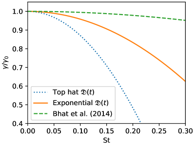
Figure 1: Growth rate as a function of $\operatorname{St}$ for two different temporal correlation functions, along with the expression obtained by [p. 4]bhat2014fluctuation.

Let us now compare the growth rates we found in section 4.3 with those reported by bhat2014fluctuation. The velocity field chosen they chose corresponds to the longitudinal correlation function

$$E^{\text{BS14}}_{L}(r)=\frac{A^{2}\tau}{6}\left[1+\frac{1}{q^{2}}\frac{\partial^{2}}{\partial r^{2}}\right]j_{0}(qr)$$ (78)

where $\tau$ is the renovation time of the velocity field, $q$ is a characteristic wavenumber, $A$ is related to the amplitude of the velocity field, and $j_{0}$ is the spherical Bessel function of the first kind of order 0 (recall that $j_{0}(z)=\operatorname{sinc}(z)$). We identify $q\equiv k_{f}$. Noting that they define

$$\eta_{t}\equiv\frac{E^{\text{BS14}}_{L}(0)}{2}=\frac{A^{2}\tau}{18}\,,\quad\overline{\tau}^{\text{BS14}}\equiv\tau\eta_{t}q^{2}=\frac{\bar{\tau}}{2}=\frac{2\operatorname{St}^{2}}{3}$$ (79)

Note that for the last equality, we have used $\bar{\tau}=4\operatorname{St}^{2}/3$ which corresponds to the temporal correlation function being a top hat. the growth rate found by them can be written as (Bhat & Subramanian, 2014, p. 4)

$$\gamma=\gamma_{0}\left(1-\frac{15\operatorname{St}^{2}}{28}\right)\approx\gamma_{0}\left(1-0.5\operatorname{St}^{2}\right)$$ (80)

This is shown in figure 1, along with the growth rates we obtained in section 4.3. The suppression of the growth rate is much stronger in our case.

Schekochihin & Kulsrud (2001, eq. 85) have derived an expression for the growth rates of the single-point moments of the magnetic field at $\operatorname{Pr}_{\mathrm{m}}\gg 1$ when $\tau_{c}\neq 0$. This expression is superficially similar to ours, in that it contains constants parametrizing the temporal correlation properties of the velocity field. However, they set $\eta=0$ at the starting of their calculations, while we have taken the limit $\eta\to 0$ only towards the end. Even when $\tau_{c}=0$, this is known to significantly affect the predicted growth rate (compare eqs. 1.9 and 1.16 of Kulsrud & Anderson, 1992), and hence we do not expect our $\mathcal{O}(\tau_{c})$ corrections to match theirs. Appendix H discusses how the quantities we have defined are related to theirs.

5 Conclusions

By assuming that the velocity field is an incompressible separable Gaussian random field, we have derived the Fourier-space evolution equation for the two-point correlation function of the magnetic field. Using this equation and further assuming that the velocity field is nonhelical, we have derived the evolution equation for the longitudinal correlation function of the magnetic field ($M_{L}$) in configuration space, valid for arbitrary $\operatorname{Pr}_{\mathrm{m}}$ (equation 28). Unlike in previous work, setting $\eta=0$ gives an evolution equation with at most two spatial derivatives of $M_{L}$.

By choosing an appropriate form for the longitudinal correlation function of the velocity field, we have studied the $\operatorname{Pr}_{\mathrm{m}}\gg 1$ limit. In agreement with previous work (Chandran, 1997; Mason et al., 2011; Bhat & Subramanian, 2014; Carteret et al., 2023; Schekochihin & Kulsrud, 2001), we have found that the growth rate of the magnetic field decreases when the correlation time is nonzero. The growth rate is suppressed much more strongly than in the renovating flow model (Bhat & Subramanian, 2014; Carteret et al., 2023). However, the corrections to the spectral slope of the magnetic field are still negligible when $\operatorname{Rm}\gg 1$.

While our equation 28 can also be used to study the limit $\operatorname{Pr}_{\mathrm{m}}\ll 1$, this seems to be more complicated than the case presented here, and will be described elsewhere. It may be interesting to study how the effects of kinetic helicity on the small-scale dynamo (Malyshkin & Boldyrev, 2007, 2010) are affected by the correlation time being nonzero.

Appendix A Furutsu-Novikov theorem

Given a functional $R[f]$ of a function $f$, its functional derivative is defined as

$$\left.\frac{\mathrm{d}^{n}R[f+\epsilon\chi]}{\mathrm{d}\epsilon^{n}}\right|_{\epsilon=0}=\int\frac{\delta^{n}R}{\delta f(s_{1})\dots\delta f(s_{n})}\,\chi(s_{1})\dots\chi(s_{n})\,\mathrm{d}s_{1}\dots\mathrm{d}s_{n}$$ (A1)

where $\epsilon$ is a real number, and $\chi(t)$ is an arbitrary test function. If $f(s)$ is a zero-mean Gaussian random function, $R[f]$ satisfies the Furutsu-Novikov formula (Furutsu, 1963; Novikov, 1965):

$$\left<f(s)R[f]\right>=\int\left<f(s)f(s_{1})\right>\left<\frac{\delta R[f]}{\delta f(s_{1})}\right>\,\mathrm{d}s_{1}$$ (A2)

Equation A2 also holds if $s$ is a collection of spatio-temporal variables and vector indices.

Appendix B The Fourier-space evolution equation

The evolution equation for the two-point single-time correlation of the magnetic field in Fourier space is

$$\begin{split}\frac{\partial\left<\mathcal{B}_{ij}^{(\boldsymbol{k},t;-\boldsymbol{k},t)}\right>}{\partial t}={}&-\eta\left|\boldsymbol{k^{\prime}}\right|^{2}\left<\mathcal{B}_{ij}^{(\boldsymbol{k},t;-\boldsymbol{k},t)}\right>+\left[\mathcal{I}^{1}\right]_{ij}^{(\boldsymbol{k},t)}+\left[\mathcal{I}^{2}\right]_{ij}^{(\boldsymbol{k},t)}+\left[\mathcal{I}^{3}\right]_{ij}^{(\boldsymbol{k},t)}+\left[\mathcal{I}^{4}\right]_{ij}^{(\boldsymbol{k},t)}+\left[\mathcal{I}^{5}\right]_{ij}^{(\boldsymbol{k},t)}\\ &+\left[i\leftrightarrow j;\,\boldsymbol{k}\to-\boldsymbol{k}\right]+\mathcal{O}(\tau_{c}^{2})\end{split}$$ (B1)

When $\tau_{c}=0$, only $\left[\mathcal{I}^{3}\right]$ and the explicit resistive term are nonzero. The terms $\left[\mathcal{I}^{1}\right]$ and $\left[\mathcal{I}^{2}\right]$ come from the second functional derivative of $\mathcal{B}$; while $\left[\mathcal{I}^{3}\right]$, $\left[\mathcal{I}^{4}\right]$, and $\left[\mathcal{I}^{5}\right]$ come from Taylor-expanding the $\left<\mathcal{B}\right>$ term that appears during the first application of equation 12 to equation 9. Using the convention that $\left[\mathcal{I}^{1}\right]=\left[\mathcal{I}^{1.1}\right]+\left[\mathcal{I}^{1.2}\right]+\dots$ and so on, the terms on the RHS of equation B1 are

$$\begin{split}\left[\mathcal{I}^{1.1}\right]_{ij}^{(\boldsymbol{k},t)}={}&\tau_{c}g_{1}\left<\mathcal{B}_{iu}^{(\boldsymbol{k},t;-\boldsymbol{k},t)}\right>\int_{\begin{subarray}{c}\boldsymbol{k}^{(1)}\end{subarray}}\mathcal{A}_{jas}^{(-\boldsymbol{k}^{(1)},-\boldsymbol{k}+\boldsymbol{k}^{(1)})}\,T_{i_{1}a}^{(\boldsymbol{k}^{(1)})}\int_{\begin{subarray}{c}\boldsymbol{p}\end{subarray}}\mathcal{A}_{smn}^{(\boldsymbol{p},-\boldsymbol{k}+\boldsymbol{k}^{(1)}-\boldsymbol{p})}\mathcal{A}_{ni_{1}l}^{(\boldsymbol{k}^{(1)},-\boldsymbol{k}-\boldsymbol{p})}\mathcal{A}_{li_{2}u}^{(-\boldsymbol{p},-\boldsymbol{k})}\,T_{mi_{2}}^{(\boldsymbol{p})}\end{split}$$ (B2)

$$\begin{split}\left[\mathcal{I}^{1.2}\right]_{ij}^{(\boldsymbol{k},t)}={}&\tau_{c}g_{1}\int_{\begin{subarray}{c}\boldsymbol{k}^{(1)},\boldsymbol{q}\end{subarray}}\operatorname{\delta}^{(\boldsymbol{k}-\boldsymbol{k}^{(1)}-\boldsymbol{q})}\mathcal{A}_{jas}^{(-\boldsymbol{k}^{(1)},-\boldsymbol{k}+\boldsymbol{k}^{(1)})}\,T_{i_{1}a}^{(\boldsymbol{k}^{(1)})}\left<\mathcal{B}_{us}^{(\boldsymbol{q},t;-\boldsymbol{q},t)}\right>\int_{\begin{subarray}{c}\boldsymbol{p}\end{subarray}}\mathcal{A}_{imn}^{(\boldsymbol{p},\boldsymbol{k}-\boldsymbol{p})}\mathcal{A}_{ni_{1}l}^{(\boldsymbol{k}^{(1)},\boldsymbol{k}-\boldsymbol{p}-\boldsymbol{k}^{(1)})}\mathcal{A}_{li_{2}u}^{(-\boldsymbol{p},\boldsymbol{k}-\boldsymbol{k}^{(1)})}\,T_{mi_{2}}^{(\boldsymbol{p})}\end{split}$$ (B3)

$$\begin{split}\left[\mathcal{I}^{1.3}\right]_{ij}^{(\boldsymbol{k},t)}={}&\tau_{c}g_{1}\int_{\begin{subarray}{c}\boldsymbol{k}^{(1)},\boldsymbol{q},\boldsymbol{p}\end{subarray}}\operatorname{\delta}^{(\boldsymbol{k}-\boldsymbol{k}^{(1)}-\boldsymbol{p}-\boldsymbol{q})}\mathcal{A}_{jbs}^{(-\boldsymbol{k}^{(1)},-\boldsymbol{k}+\boldsymbol{k}^{(1)})}\,T_{i_{1}b}^{(\boldsymbol{k}^{(1)})}\\ &\phantom{===}\times\mathcal{A}_{sma}^{(-\boldsymbol{p},-\boldsymbol{k}+\boldsymbol{k}^{(1)}+\boldsymbol{p})}\mathcal{A}_{ii_{1}l}^{(\boldsymbol{k}^{(1)},\boldsymbol{k}-\boldsymbol{k}^{(1)})}\mathcal{A}_{li_{2}u}^{(\boldsymbol{p},\boldsymbol{k}-\boldsymbol{k}^{(1)}-\boldsymbol{p})}\,T_{i_{2}m}^{(\boldsymbol{p})}\left<\mathcal{B}_{ua}^{(\boldsymbol{q},t;-\boldsymbol{q},t)}\right>\end{split}$$ (B4)

$$\begin{split}\left[\mathcal{I}^{1.4}\right]_{ij}^{(\boldsymbol{k},t)}={}&\tau_{c}g_{1}\int_{\begin{subarray}{c}\boldsymbol{p},\boldsymbol{q}\end{subarray}}\operatorname{\delta}^{(\boldsymbol{k}-\boldsymbol{p}-\boldsymbol{q})}\mathcal{A}_{ima}^{(\boldsymbol{p},\boldsymbol{k}-\boldsymbol{p})}\mathcal{A}_{li_{2}u}^{(-\boldsymbol{p},-\boldsymbol{k}+\boldsymbol{p})}\,T_{mi_{2}}^{(\boldsymbol{p})}\left<\mathcal{B}_{au}^{(\boldsymbol{q},t;-\boldsymbol{q},t)}\right>\int_{\begin{subarray}{c}\boldsymbol{k}^{(1)}\end{subarray}}\mathcal{A}_{jbs}^{(-\boldsymbol{k}^{(1)},-\boldsymbol{k}+\boldsymbol{k}^{(1)})}\mathcal{A}_{si_{1}l}^{(\boldsymbol{k}^{(1)},-\boldsymbol{k})}\,T_{i_{1}b}^{(\boldsymbol{k}^{(1)})}\end{split}$$ (B5)

$$\begin{split}\left[\mathcal{I}^{1.5}\right]_{ij}^{(\boldsymbol{k},t)}={}&\tau_{c}g_{1}\int_{\begin{subarray}{c}\boldsymbol{p},\boldsymbol{q}\end{subarray}}\operatorname{\delta}^{(\boldsymbol{k}-\boldsymbol{p}-\boldsymbol{q})}\mathcal{A}_{ii_{2}u}^{(\boldsymbol{p},\boldsymbol{k}-\boldsymbol{p})}\,T_{i_{2}m}^{(\boldsymbol{p})}\left<\mathcal{B}_{ua}^{(\boldsymbol{q},t;-\boldsymbol{q},t)}\right>\int_{\begin{subarray}{c}\boldsymbol{k}^{(1)}\end{subarray}}\mathcal{A}_{smn}^{(-\boldsymbol{p},-\boldsymbol{k}+\boldsymbol{k}^{(1)}+\boldsymbol{p})}\mathcal{A}_{ni_{1}a}^{(\boldsymbol{k}^{(1)},-\boldsymbol{k}+\boldsymbol{p})}\mathcal{A}_{jbs}^{(-\boldsymbol{k}^{(1)},-\boldsymbol{k}+\boldsymbol{k}^{(1)})}\,T_{i_{1}b}^{(\boldsymbol{k}^{(1)})}\end{split}$$ (B6)

$$\begin{split}\left[\mathcal{I}^{1.6}\right]_{ij}^{(\boldsymbol{k},t)}={}&\tau_{c}g_{1}\int_{\begin{subarray}{c}\boldsymbol{k}^{(1)},\boldsymbol{p},\boldsymbol{q}\end{subarray}}\operatorname{\delta}^{(\boldsymbol{k}-\boldsymbol{p}-\boldsymbol{k}^{(1)}-\boldsymbol{q})}\mathcal{A}_{jbs}^{(-\boldsymbol{k}^{(1)},-\boldsymbol{k}+\boldsymbol{k}^{(1)})}\,T_{i_{1}b}^{(\boldsymbol{k}^{(1)})}\\ &\phantom{===}\times\mathcal{A}_{imn}^{(\boldsymbol{p},\boldsymbol{k}-\boldsymbol{p})}\mathcal{A}_{ni_{1}a}^{(\boldsymbol{k}^{(1)},\boldsymbol{k}-\boldsymbol{p}-\boldsymbol{k}^{(1)})}\mathcal{A}_{si_{2}u}^{(-\boldsymbol{p},-\boldsymbol{k}+\boldsymbol{k}^{(1)}+\boldsymbol{p})}\,T_{mi_{2}}^{(\boldsymbol{p})}\left<\mathcal{B}_{au}^{(\boldsymbol{q},t;-\boldsymbol{q},t)}\right>\end{split}$$ (B7)

$$\begin{split}\left[\mathcal{I}^{1.7}\right]_{ij}^{(\boldsymbol{k},t)}={}&\tau_{c}g_{1}\int_{\begin{subarray}{c}\boldsymbol{k}^{(1)},\boldsymbol{q}\end{subarray}}\operatorname{\delta}^{(\boldsymbol{k}-\boldsymbol{k}^{(1)}-\boldsymbol{q})}\mathcal{A}_{jbs}^{(-\boldsymbol{k}^{(1)},-\boldsymbol{k}+\boldsymbol{k}^{(1)})}\,T_{i_{1}b}^{(\boldsymbol{k}^{(1)})}\left<\mathcal{B}_{au}^{(\boldsymbol{q},t;-\boldsymbol{q},t)}\right>\\ &\phantom{===}\times\int_{\begin{subarray}{c}\boldsymbol{p}\end{subarray}}\mathcal{A}_{sml}^{(\boldsymbol{p},-\boldsymbol{k}+\boldsymbol{k}^{(1)}-\boldsymbol{p})}\mathcal{A}_{ii_{1}a}^{(\boldsymbol{k}^{(1)},\boldsymbol{k}-\boldsymbol{k}^{(1)})}\mathcal{A}_{li_{2}u}^{(-\boldsymbol{p},-\boldsymbol{k}+\boldsymbol{k}^{(1)})}\,T_{mi_{2}}^{(\boldsymbol{p})}\end{split}$$ (B8)

$$\begin{split}\left[\mathcal{I}^{1.8}\right]_{ij}^{(\boldsymbol{k},t)}={}&\tau_{c}g_{1}\left<\mathcal{B}_{ua}^{(\boldsymbol{k},t;-\boldsymbol{k},t)}\right>\int_{\begin{subarray}{c}\boldsymbol{k}^{(1)}\end{subarray}}\mathcal{A}_{jbs}^{(-\boldsymbol{k}^{(1)},-\boldsymbol{k}+\boldsymbol{k}^{(1)})}\,T_{i_{1}b}^{(\boldsymbol{k}^{(1)})}\int_{\begin{subarray}{c}\boldsymbol{p}\end{subarray}}\mathcal{A}_{iml}^{(\boldsymbol{p},\boldsymbol{k}-\boldsymbol{p})}\mathcal{A}_{si_{1}a}^{(\boldsymbol{k}^{(1)},-\boldsymbol{k})}\mathcal{A}_{li_{2}u}^{(-\boldsymbol{p},\boldsymbol{k})}\,T_{mi_{2}}^{(\boldsymbol{p})}\end{split}$$ (B9)

$$\begin{split}\left[\mathcal{I}^{2.1}\right]_{ij}^{(\boldsymbol{k},t)}={}&\tau_{c}g_{2}\left<\mathcal{B}_{iu}^{(\boldsymbol{k},t;-\boldsymbol{k},t)}\right>\int_{\begin{subarray}{c}\boldsymbol{k}^{(1)}\end{subarray}}\mathcal{A}_{jas}^{(-\boldsymbol{k}^{(1)},-\boldsymbol{k}+\boldsymbol{k}^{(1)})}\,T_{i_{1}a}^{(\boldsymbol{k}^{(1)})}\int_{\begin{subarray}{c}\boldsymbol{p}\end{subarray}}\mathcal{A}_{smn}^{(\boldsymbol{p},-\boldsymbol{k}+\boldsymbol{k}^{(1)}-\boldsymbol{p})}\mathcal{A}_{ni_{2}l}^{(-\boldsymbol{p},-\boldsymbol{k}+\boldsymbol{k}^{(1)})}\mathcal{A}_{li_{1}u}^{(\boldsymbol{k}^{(1)},-\boldsymbol{k})}\,T_{mi_{2}}^{(\boldsymbol{p})}\end{split}$$ (B10)

$$\begin{split}\left[\mathcal{I}^{2.2}\right]_{ij}^{(\boldsymbol{k},t)}={}&\tau_{c}g_{2}\int_{\begin{subarray}{c}\boldsymbol{k}^{(1)},\boldsymbol{q}\end{subarray}}\operatorname{\delta}^{(\boldsymbol{k}-\boldsymbol{k}^{(1)}-\boldsymbol{q})}\mathcal{A}_{jas}^{(-\boldsymbol{k}^{(1)},-\boldsymbol{k}+\boldsymbol{k}^{(1)})}\,T_{i_{1}a}^{(\boldsymbol{k}^{(1)})}\left<\mathcal{B}_{us}^{(\boldsymbol{q},t;-\boldsymbol{q},t)}\right>\int_{\begin{subarray}{c}\boldsymbol{p}\end{subarray}}\mathcal{A}_{imn}^{(\boldsymbol{p},\boldsymbol{k}-\boldsymbol{p})}\mathcal{A}_{ni_{2}l}^{(-\boldsymbol{p},\boldsymbol{k})}\mathcal{A}_{li_{1}u}^{(\boldsymbol{k}^{(1)},\boldsymbol{k}-\boldsymbol{k}^{(1)})}\,T_{mi_{2}}^{(\boldsymbol{p})}\end{split}$$ (B11)

$$\begin{split}\left[\mathcal{I}^{2.3}\right]_{ij}^{(\boldsymbol{k},t)}={}&\tau_{c}g_{2}\int_{\begin{subarray}{c}\boldsymbol{k}^{(1)},\boldsymbol{p},\boldsymbol{q}\end{subarray}}\operatorname{\delta}^{(\boldsymbol{k}-\boldsymbol{p}-\boldsymbol{k}^{(1)}-\boldsymbol{q})}\mathcal{A}_{jbs}^{(-\boldsymbol{k}^{(1)},-\boldsymbol{k}+\boldsymbol{k}^{(1)})}\,T_{i_{1}b}^{(\boldsymbol{k}^{(1)})}\mathcal{A}_{sma}^{(-\boldsymbol{p},-\boldsymbol{k}+\boldsymbol{k}^{(1)}+\boldsymbol{p})}\\ &\phantom{===}\times\mathcal{A}_{ii_{2}l}^{(\boldsymbol{p},\boldsymbol{k}-\boldsymbol{p})}\mathcal{A}_{li_{1}u}^{(\boldsymbol{k}^{(1)},\boldsymbol{k}-\boldsymbol{p}-\boldsymbol{k}^{(1)})}\,T_{i_{2}m}^{(\boldsymbol{p})}\left<\mathcal{B}_{ua}^{(\boldsymbol{q},t;-\boldsymbol{q},t)}\right>\end{split}$$ (B12)

$$\begin{split}\left[\mathcal{I}^{2.4}\right]_{ij}^{(\boldsymbol{k},t)}={}&\tau_{c}g_{2}\int_{\begin{subarray}{c}\boldsymbol{p},\boldsymbol{q}\end{subarray}}\operatorname{\delta}^{(\boldsymbol{k}-\boldsymbol{p}-\boldsymbol{q})}\mathcal{A}_{ima}^{(\boldsymbol{p},\boldsymbol{k}-\boldsymbol{p})}\,T_{mi_{2}}^{(\boldsymbol{p})}\left<\mathcal{B}_{au}^{(\boldsymbol{q},t;-\boldsymbol{q},t)}\right>\int_{\begin{subarray}{c}\boldsymbol{k}^{(1)}\end{subarray}}\mathcal{A}_{si_{2}l}^{(-\boldsymbol{p},-\boldsymbol{k}+\boldsymbol{k}^{(1)}+\boldsymbol{p})}\mathcal{A}_{li_{1}u}^{(\boldsymbol{k}^{(1)},-\boldsymbol{k}+\boldsymbol{p})}\mathcal{A}_{jbs}^{(-\boldsymbol{k}^{(1)},-\boldsymbol{k}+\boldsymbol{k}^{(1)})}\,T_{i_{1}b}^{(\boldsymbol{k}^{(1)})}\end{split}$$ (B13)

$$\begin{split}\left[\mathcal{I}^{2.5}\right]_{ij}^{(\boldsymbol{k},t)}={}&\tau_{c}g_{2}\int_{\begin{subarray}{c}\boldsymbol{k}^{(1)},\boldsymbol{q}\end{subarray}}\operatorname{\delta}^{(\boldsymbol{k}-\boldsymbol{k}^{(1)}-\boldsymbol{q})}\mathcal{A}_{jbs}^{(-\boldsymbol{k}^{(1)},-\boldsymbol{k}+\boldsymbol{k}^{(1)})}\,T_{i_{1}b}^{(\boldsymbol{k}^{(1)})}\left<\mathcal{B}_{ua}^{(\boldsymbol{q},t;-\boldsymbol{q},t)}\right>\\ &\phantom{===}\times\int_{\begin{subarray}{c}\boldsymbol{p}\end{subarray}}\mathcal{A}_{smn}^{(\boldsymbol{p},-\boldsymbol{k}+\boldsymbol{k}^{(1)}-\boldsymbol{p})}\mathcal{A}_{ni_{2}a}^{(-\boldsymbol{p},-\boldsymbol{k}+\boldsymbol{k}^{(1)})}\mathcal{A}_{ii_{1}u}^{(\boldsymbol{k}^{(1)},\boldsymbol{k}-\boldsymbol{k}^{(1)})}\,T_{mi_{2}}^{(\boldsymbol{p})}\end{split}$$ (B14)

$$\begin{split}\left[\mathcal{I}^{2.6}\right]_{ij}^{(\boldsymbol{k},t)}={}&\tau_{c}g_{2}\left<\mathcal{B}_{au}^{(\boldsymbol{k},t;-\boldsymbol{k},t)}\right>\int_{\begin{subarray}{c}\boldsymbol{k}^{(1)}\end{subarray}}\mathcal{A}_{jbs}^{(-\boldsymbol{k}^{(1)},-\boldsymbol{k}+\boldsymbol{k}^{(1)})}\,T_{i_{1}b}^{(\boldsymbol{k}^{(1)})}\int_{\begin{subarray}{c}\boldsymbol{p}\end{subarray}}\mathcal{A}_{imn}^{(\boldsymbol{p},\boldsymbol{k}-\boldsymbol{p})}\mathcal{A}_{ni_{2}a}^{(-\boldsymbol{p},\boldsymbol{k})}\mathcal{A}_{si_{1}u}^{(\boldsymbol{k}^{(1)},-\boldsymbol{k})}\,T_{mi_{2}}^{(\boldsymbol{p})}\end{split}$$ (B15)

$$\begin{split}\left[\mathcal{I}^{2.7}\right]_{ij}^{(\boldsymbol{k},t)}={}&\tau_{c}g_{2}\int_{\begin{subarray}{c}\boldsymbol{p},\boldsymbol{q}\end{subarray}}\operatorname{\delta}^{(\boldsymbol{k}-\boldsymbol{p}-\boldsymbol{q})}\mathcal{A}_{ii_{2}a}^{(\boldsymbol{p},\boldsymbol{k}-\boldsymbol{p})}\,T_{i_{2}m}^{(\boldsymbol{p})}\left<\mathcal{B}_{au}^{(\boldsymbol{q},t;-\boldsymbol{q},t)}\right>\int_{\begin{subarray}{c}\boldsymbol{k}^{(1)}\end{subarray}}\mathcal{A}_{sml}^{(-\boldsymbol{p},-\boldsymbol{k}+\boldsymbol{k}^{(1)}+\boldsymbol{p})}\mathcal{A}_{li_{1}u}^{(\boldsymbol{k}^{(1)},-\boldsymbol{k}+\boldsymbol{p})}\mathcal{A}_{jbs}^{(-\boldsymbol{k}^{(1)},-\boldsymbol{k}+\boldsymbol{k}^{(1)})}\,T_{i_{1}b}^{(\boldsymbol{k}^{(1)})}\end{split}$$ (B16)

$$\begin{split}\left[\mathcal{I}^{2.8}\right]_{ij}^{(\boldsymbol{k},t)}={}&\tau_{c}g_{2}\int_{\begin{subarray}{c}\boldsymbol{k}^{(1)},\boldsymbol{p},\boldsymbol{q}\end{subarray}}\operatorname{\delta}^{(\boldsymbol{k}-\boldsymbol{p}-\boldsymbol{k}^{(1)}-\boldsymbol{q})}\mathcal{A}_{jbs}^{(-\boldsymbol{k}^{(1)},-\boldsymbol{k}+\boldsymbol{k}^{(1)})}\,T_{i_{1}b}^{(\boldsymbol{k}^{(1)})}\\ &\phantom{===}\times\mathcal{A}_{iml}^{(\boldsymbol{p},\boldsymbol{k}-\boldsymbol{p})}\mathcal{A}_{si_{2}a}^{(-\boldsymbol{p},-\boldsymbol{k}+\boldsymbol{k}^{(1)}+\boldsymbol{p})}\mathcal{A}_{li_{1}u}^{(\boldsymbol{k}^{(1)},\boldsymbol{k}-\boldsymbol{p}-\boldsymbol{k}^{(1)})}\,T_{mi_{2}}^{(\boldsymbol{p})}\left<\mathcal{B}_{ua}^{(\boldsymbol{q},t;-\boldsymbol{q},t)}\right>\end{split}$$ (B17)

$$\begin{split}\left[\mathcal{I}^{3.1}\right]_{ij}^{(\boldsymbol{k},t)}={}&\left<\mathcal{B}_{in}^{(\boldsymbol{k},t;-\boldsymbol{k},t)}\right>\int_{\begin{subarray}{c}\boldsymbol{k}^{(1)}\end{subarray}}\mathcal{A}_{jas}^{(-\boldsymbol{k}^{(1)},-\boldsymbol{k}+\boldsymbol{k}^{(1)})}\,T_{i_{1}a}^{(\boldsymbol{k}^{(1)})}\mathcal{A}_{si_{1}n}^{(\boldsymbol{k}^{(1)},-\boldsymbol{k})}\left[\frac{1}{2}+\frac{\tau_{c}\eta}{2}\left(-\left|\boldsymbol{k}^{(1)}-\boldsymbol{k}\right|^{2}+\left|\boldsymbol{k}\right|^{2}\right)\right]\end{split}$$ (B18)

$$\begin{split}\left[\mathcal{I}^{3.2}\right]_{ij}^{(\boldsymbol{k},t)}={}&\int_{\begin{subarray}{c}\boldsymbol{k}^{(1)},\boldsymbol{q}\end{subarray}}\operatorname{\delta}^{(\boldsymbol{k}-\boldsymbol{k}^{(1)}-\boldsymbol{q})}\mathcal{A}_{jas}^{(-\boldsymbol{k}^{(1)},-\boldsymbol{k}+\boldsymbol{k}^{(1)})}\,T_{i_{1}a}^{(\boldsymbol{k}^{(1)})}\mathcal{A}_{ii_{1}n}^{(\boldsymbol{k}^{(1)},\boldsymbol{k}-\boldsymbol{k}^{(1)})}\left[\frac{1}{2}+\frac{\tau_{c}\eta}{2}\left(-\left|\boldsymbol{k}\right|^{2}+\left|\boldsymbol{k}-\boldsymbol{k}^{(1)}\right|^{2}\right)\right]\left<\mathcal{B}_{ns}^{(\boldsymbol{q},t;-\boldsymbol{q},t)}\right>\end{split}$$ (B19)

$$\begin{split}\left[\mathcal{I}^{4.1}\right]_{ij}^{(\boldsymbol{k},t)}={}&-\frac{\tau_{c}}{4}\left<\mathcal{B}_{ib}^{(\boldsymbol{k},t;-\boldsymbol{k},t)}\right>\int_{\begin{subarray}{c}\boldsymbol{k}^{(1)}\end{subarray}}\mathcal{A}_{jms}^{(-\boldsymbol{k}^{(1)},-\boldsymbol{k}+\boldsymbol{k}^{(1)})}\,T_{i_{1}m}^{(\boldsymbol{k}^{(1)})}\mathcal{A}_{si_{1}n}^{(\boldsymbol{k}^{(1)},-\boldsymbol{k})}\int_{\begin{subarray}{c}\boldsymbol{p}\end{subarray}}\mathcal{A}_{nla}^{(\boldsymbol{p},-\boldsymbol{k}-\boldsymbol{p})}\,T_{li_{2}}^{(\boldsymbol{p})}\mathcal{A}_{ai_{2}b}^{(-\boldsymbol{p},-\boldsymbol{k})}\end{split}$$ (B20)

$$\begin{split}\left[\mathcal{I}^{4.2}\right]_{ij}^{(\boldsymbol{k},t)}={}&-\frac{\tau_{c}}{4}\int_{\begin{subarray}{c}\boldsymbol{k}^{(1)},\boldsymbol{q}\end{subarray}}\operatorname{\delta}^{(\boldsymbol{k}-\boldsymbol{k}^{(1)}-\boldsymbol{q})}\mathcal{A}_{jms}^{(-\boldsymbol{k}^{(1)},-\boldsymbol{k}+\boldsymbol{k}^{(1)})}\,T_{i_{1}m}^{(\boldsymbol{k}^{(1)})}\left<\mathcal{B}_{bs}^{(\boldsymbol{q},t;-\boldsymbol{q},t)}\right>\\ &\phantom{===}\times\int_{\begin{subarray}{c}\boldsymbol{p}\end{subarray}}\mathcal{A}_{ii_{1}n}^{(\boldsymbol{k}^{(1)},\boldsymbol{k}-\boldsymbol{k}^{(1)})}\mathcal{A}_{nla}^{(\boldsymbol{p},\boldsymbol{k}-\boldsymbol{k}^{(1)}-\boldsymbol{p})}\,T_{li_{2}}^{(\boldsymbol{p})}\mathcal{A}_{ai_{2}b}^{(-\boldsymbol{p},\boldsymbol{k}-\boldsymbol{k}^{(1)})}\end{split}$$ (B21)

$$\begin{split}\left[\mathcal{I}^{4.3}\right]_{ij}^{(\boldsymbol{k},t)}={}&-\frac{\tau_{c}}{4}\left<\mathcal{B}_{bm}^{(\boldsymbol{k},t;-\boldsymbol{k},t)}\right>\int_{\begin{subarray}{c}\boldsymbol{k}^{(1)}\end{subarray}}\mathcal{A}_{jns}^{(-\boldsymbol{k}^{(1)},-\boldsymbol{k}+\boldsymbol{k}^{(1)})}\,T_{i_{1}n}^{(\boldsymbol{k}^{(1)})}\mathcal{A}_{si_{1}m}^{(\boldsymbol{k}^{(1)},-\boldsymbol{k})}\int_{\begin{subarray}{c}\boldsymbol{p}\end{subarray}}\mathcal{A}_{ila}^{(\boldsymbol{p},\boldsymbol{k}-\boldsymbol{p})}\,T_{li_{2}}^{(\boldsymbol{p})}\mathcal{A}_{ai_{2}b}^{(-\boldsymbol{p},\boldsymbol{k})}\end{split}$$ (B22)

$$\begin{split}\left[\mathcal{I}^{4.4}\right]_{ij}^{(\boldsymbol{k},t)}={}&-\frac{\tau_{c}}{4}\int_{\begin{subarray}{c}\boldsymbol{k}^{(1)},\boldsymbol{q}\end{subarray}}\operatorname{\delta}^{(\boldsymbol{k}-\boldsymbol{k}^{(1)}-\boldsymbol{q})}\mathcal{A}_{jns}^{(-\boldsymbol{k}^{(1)},-\boldsymbol{k}+\boldsymbol{k}^{(1)})}\,T_{i_{1}n}^{(\boldsymbol{k}^{(1)})}\mathcal{A}_{ii_{1}m}^{(\boldsymbol{k}^{(1)},\boldsymbol{k}-\boldsymbol{k}^{(1)})}\left<\mathcal{B}_{mb}^{(\boldsymbol{q},t;-\boldsymbol{q},t)}\right>\\ &\phantom{===}\times\int_{\begin{subarray}{c}\boldsymbol{p}\end{subarray}}\mathcal{A}_{sla}^{(\boldsymbol{p},-\boldsymbol{k}+\boldsymbol{k}^{(1)}-\boldsymbol{p})}\,T_{li_{2}}^{(\boldsymbol{p})}\mathcal{A}_{ai_{2}b}^{(-\boldsymbol{p},-\boldsymbol{k}+\boldsymbol{k}^{(1)})}\end{split}$$ (B23)

$$\begin{split}\left[\mathcal{I}^{5.1}\right]_{ij}^{(\boldsymbol{k},t)}={}&-\frac{\tau_{c}}{2}\int_{\begin{subarray}{c}\boldsymbol{p},\boldsymbol{q}\end{subarray}}\operatorname{\delta}^{(\boldsymbol{k}-\boldsymbol{p}-\boldsymbol{q})}\mathcal{A}_{nla}^{(-\boldsymbol{p},-\boldsymbol{k}+\boldsymbol{p})}\,T_{i_{2}l}^{(\boldsymbol{p})}\mathcal{A}_{ii_{2}b}^{(\boldsymbol{p},\boldsymbol{k}-\boldsymbol{p})}\left<\mathcal{B}_{ba}^{(\boldsymbol{q},t;-\boldsymbol{q},t)}\right>\int_{\begin{subarray}{c}\boldsymbol{k}^{(1)}\end{subarray}}\mathcal{A}_{si_{1}n}^{(\boldsymbol{k}^{(1)},-\boldsymbol{k})}\mathcal{A}_{jms}^{(-\boldsymbol{k}^{(1)},-\boldsymbol{k}+\boldsymbol{k}^{(1)})}\,T_{i_{1}m}^{(\boldsymbol{k}^{(1)})}\end{split}$$ (B24)

$$\begin{split}\left[\mathcal{I}^{5.2}\right]_{ij}^{(\boldsymbol{k},t)}={}&-\frac{\tau_{c}}{2}\int_{\begin{subarray}{c}\boldsymbol{k}^{(1)},\boldsymbol{p},\boldsymbol{q}\end{subarray}}\operatorname{\delta}^{(\boldsymbol{k}-\boldsymbol{k}^{(1)}-\boldsymbol{p}-\boldsymbol{q})}\mathcal{A}_{jms}^{(-\boldsymbol{k}^{(1)},-\boldsymbol{k}+\boldsymbol{k}^{(1)})}\,T_{i_{1}m}^{(\boldsymbol{k}^{(1)})}\mathcal{A}_{ii_{1}n}^{(\boldsymbol{k}^{(1)},\boldsymbol{k}-\boldsymbol{k}^{(1)})}\\ &\phantom{===}\times\mathcal{A}_{nla}^{(\boldsymbol{p},\boldsymbol{k}-\boldsymbol{k}^{(1)}-\boldsymbol{p})}\,T_{li_{2}}^{(\boldsymbol{p})}\mathcal{A}_{si_{2}b}^{(-\boldsymbol{p},-\boldsymbol{k}+\boldsymbol{k}^{(1)}+\boldsymbol{p})}\left<\mathcal{B}_{ab}^{(\boldsymbol{q},t;-\boldsymbol{q},t)}\right>\end{split}$$ (B25)

Appendix C A relation between the coefficients parametrizing the temporal correlation function

Recalling the definitions of $g_{1}$ and $g_{2}$ (equations 17), we note that

$$\begin{split}g_{1}+g_{2}={}&\frac{1}{\tau_{c}}\int_{-\infty}^{t}\mathrm{d}t^{\prime}\int_{-\infty}^{t^{\prime}}\mathrm{d}t_{1}\int_{-\infty}^{t^{\prime}}\mathrm{d}t_{2}\,\mathfrak{D}^{(t-t_{1})}\mathfrak{D}^{(t^{\prime}-t_{2})}\end{split}$$ (C1)

$$\begin{split}={}&\frac{1}{2\tau_{c}}\int_{-\infty}^{t}\mathrm{d}t^{\prime}\int_{-\infty}^{t^{\prime}}\mathrm{d}t_{1}\,\mathfrak{D}^{(t-t_{1})}\end{split}$$ (C2)

$$\begin{split}={}&\frac{1}{2\tau_{c}}\int_{-\infty}^{t}\mathrm{d}t_{1}\int_{t_{1}}^{t}\mathrm{d}t^{\prime}\,\mathfrak{D}^{(t-t_{1})}\end{split}$$ (C3)

$$\begin{split}={}&\frac{1}{2\tau_{c}}\int_{-\infty}^{t}\mathrm{d}t_{1}\left(t-t_{1}\right)\mathfrak{D}^{(t-t_{1})}\end{split}$$ (C4)

$$\begin{split}={}&\frac{1}{4}\end{split}$$ (C5)

where we have used the properties of $\mathfrak{D}(\tau)$, given in equation 5.

Appendix D The relation between $M_{L}(r)$ and $M(r)$

Let us denote the lower limit of the integral in equation 23 as $r=a$. Plugging equation 21 into the RHS of equation 23 and requiring the resulting equation to hold gives us $\lim_{r\to a}r^{3}M_{L}(r)=0$. In general, this is only expected to hold for $a=0$ and $a=\infty$.

Alternatively, taking the $r\to 0$ limit of equation 23 gives us $\left[r^{3}M_{L}(r)\right]_{r\to 0}=\int_{a}^{0}r^{2}M_{ii}\,\mathrm{d}r$. Regardless of the value of $a$, equation 21 implies

$$\left<h_{i}(\boldsymbol{r},t)\,h_{i}(\boldsymbol{r},t)\right>=3M_{L}(0)$$ (D1)

as long as $\left[r\,\partial M_{L}(r)/\partial r\right]_{r=0}=0$. This tells us that if the magnetic energy is finite, $M_{L}(0)$ is also finite. This means we need $\int_{a}^{0}r^{2}M_{ii}\,\mathrm{d}r=0$. Recalling that $\int_{0}^{\infty}r^{2}M_{ii}\,\mathrm{d}r\propto M_{ii}(k=0)$, we see that this condition is satisfied by $a\to\infty$ only if $M_{ii}(k=0)=0$. On the other hand, it is trivially satisfied by $a=0$.

As far as the evolution equation for $M_{L}(r)$ in nonhelical turbulence (equation F1 or 28) is concerned, the only effect of choosing $a=\infty$ rather than $a=0$ is a change in the form of the extra terms given in equation 31. Elimination of these extra terms is possible in both cases: for $a=\infty$, one requires all the correlation functions to decay faster than any polynomial as $r\to\infty$; for $a=0$, one requires $\left[\mathrm{d}E_{L}(r)/\mathrm{d}r\right]_{r=0}=0$. Both these requirements seem reasonable.

Appendix E Fourier identities

We use the following identities (assuming $f(k)\to f(r)$, with the arrow denoting inverse Fourier transformation from $\boldsymbol{k}$ to $\boldsymbol{r}$; note the second identity holds when $f$ is independent of the direction of $\boldsymbol{k}$):

$$k_{i}f(k)\to i\,\frac{\partial f(r)}{\partial r_{i}}\,,\quad k^{2}f(k)\to-\frac{1}{r^{2}}\,\frac{\mathrm{d}}{\mathrm{d}r}{\left(r^{2}\,\frac{\mathrm{d}f(r)}{\mathrm{d}r}\right)}$$ (E1)

Further assuming that $f(r=\infty)=0$, we write

$$\begin{split}\frac{f(k)}{k^{2}}\to{}&-\int_{r}^{\infty}\left(\frac{\mathrm{d}r}{r^{2}}\int_{r}^{\infty}\mathrm{d}r\,r^{2}f(r)\right)\end{split}$$ (E2)

Appendix F The evolution equation in real space with fourth-order derivatives

$$\begin{split}\frac{\partial M_{L}}{\partial t}={}&\frac{1}{r^{4}}\,\frac{\partial}{\partial r}{\left(\left[\kappa(r)+\tau_{c}\,\chi_{\tau}(r)\right]r^{4}\,\frac{\partial M_{L}}{\partial r}\right)}+\left[G(r)+\tau_{c}\,\mathcal{G}_{\tau}(r)\right]M_{L}+\tau_{c}\,A(r)\,\frac{\partial M_{L}}{\partial r}\\ &+2\tau_{c}\left(\frac{\eta}{2}\,\frac{\mathrm{d}S_{2}}{\mathrm{d}r}+\frac{g}{r^{4}}\,\frac{\mathrm{d}{\left(r^{4}S_{2}^{2}\right)}}{\mathrm{d}r}\right)\frac{\partial^{3}M_{L}}{\partial r^{3}}+\tau_{c}g\,S_{2}^{2}(r)\,\frac{\partial^{4}M_{L}}{\partial r^{4}}+\mathcal{O}(\tau_{c}^{2})\end{split}$$ (F1)

where we have defined $g\equiv g_{1}+g_{2}-1/4$ (in appendix C, we show that this quantity is actually zero) and

$$\begin{split}\chi_{\tau}(r)\equiv{}&g\left[-\frac{11}{4}\left(\frac{\mathrm{d}S_{2}}{\mathrm{d}r}\right)^{2}+\frac{9}{4}\,\frac{\mathrm{d}^{2}{\left(S_{2}^{2}\right)}}{\mathrm{d}r^{2}}+\frac{13}{r}\,\frac{\mathrm{d}{\left(S_{2}^{2}\right)}}{\mathrm{d}r}+\frac{8}{r^{2}}\,S_{2}^{2}{\left(r\right)}\right]+\kappa_{\tau}(r)\end{split}$$ (F2)

$$\begin{split}\mathcal{G}_{\tau}(r)\equiv{}&g\Bigg{[}\frac{S_{2}{\left(r\right)}S_{2}^{\prime\prime\prime\prime}{\left(r\right)}}{2}-\frac{S_{2}^{\prime}{\left(r\right)}S_{2}^{\prime\prime\prime}{\left(r\right)}}{2}+\frac{4S_{2}{\left(r\right)}S_{2}^{\prime\prime\prime}{\left(r\right)}}{r}+\frac{2S_{2}^{\prime}{\left(r\right)}S_{2}^{\prime\prime}{\left(r\right)}}{r}+\frac{4S_{2}{\left(r\right)}S_{2}^{\prime\prime}{\left(r\right)}}{r^{2}}\\ &\phantom{===}+\frac{8\left(S_{2}^{\prime}{\left(r\right)}\right)^{2}}{r^{2}}-\frac{4S_{2}{\left(r\right)}S_{2}^{\prime}{\left(r\right)}}{r^{3}}\Bigg{]}+G_{\tau}(r)\end{split}$$ (F3)

$$\begin{split}A(r)\equiv{}&-\frac{4\eta}{r^{5}}\,\frac{\mathrm{d}}{\mathrm{d}r}{\left(r^{4}\,\frac{\mathrm{d}S_{2}}{\mathrm{d}r}\right)}-g\left(\frac{\mathrm{d}^{3}{\left(S_{2}^{2}\right)}}{\mathrm{d}r^{3}}+\frac{12}{r}\,\frac{\mathrm{d}^{2}{\left(S_{2}^{2}\right)}}{\mathrm{d}r^{2}}+\frac{36}{r^{2}}\,\frac{\mathrm{d}{\left(S_{2}^{2}\right)}}{\mathrm{d}r}+\frac{24}{r^{3}}\,S_{2}^{2}{\left(r\right)}\right)\end{split}$$ (F4)

The rest of the quantities appearing above are defined in equations 29.

Appendix G Dimensionless numbers for a separable velocity correlation function

Given a separable velocity correlation function (see equation 5) with longitudinal correlation function $E_{L}(r)$ and temporal correlation function $\mathfrak{D}(t)$, equation 27 can be written as

$$u_{\text{rms}}^{2}=3\,E_{L}(0)\,\mathfrak{D}(0)$$ (G1)

Let us assume the velocity correlation is characterized by a length scale $1/k_{f}$. We then write

$$\operatorname{St}=\tau_{c}u_{\text{rms}}k_{f}=\tau_{c}k_{f}\sqrt{3\,E_{L}(0)\,\mathfrak{D}(0)}$$ (G2)

and

$$\operatorname{Rm}=\frac{u_{\text{rms}}}{\eta k_{f}}=\frac{\sqrt{3\,E_{L}(0)\,\mathfrak{D}(0)}}{\eta k_{f}}$$ (G3)

For example, exponential temporal correlation (see table 1) would give us

$$\tau_{c}=\frac{2\operatorname{St}^{2}}{3k_{f}^{2}\,E_{L}(0)}\,,\quad\eta=\frac{3\,E_{L}(0)}{2\operatorname{Rm}\operatorname{St}}$$ (G4)

While the numerical factors above depend on the functional form of $\mathfrak{D}(t)$, we expect $\tau_{c}\sim\operatorname{St}^{2}$ and $\eta\sim 1/(\operatorname{Rm}\operatorname{St})$ to always be valid. Schekochihin & Kulsrud (2001, eq. 95) and Bhat & Subramanian (2014, p. 3) agree that $\bar{\tau}\propto\operatorname{St}^{2}$.

Appendix H Relation with a previous calculation of the non-diffusive growth rate of single-point moments

For the sake of completeness, we note the correspondences between our work and that of Schekochihin & Kulsrud (2001). Their equation 47 for the two-point correlation of the velocity field is

$$\begin{split}\left<u_{i}^{(\boldsymbol{x}+\boldsymbol{r},t+\tau)}\,u_{j}^{(\boldsymbol{x},t)}\right>={}&\kappa_{0}^{(\tau)}\delta_{ij}-\frac{1}{2}\,\kappa_{2}^{(\tau)}\left[r^{2}\delta_{ij}+2a\,r_{i}r_{j}\right]+\frac{1}{4}\,\kappa_{4}^{(\tau)}r^{2}\left[r^{2}\delta_{ij}+2b\,r_{i}r_{j}\right]+\dots\end{split}$$ (H1)

which is more general than the form we have assumed. Incompressibility can be imposed by choosing $a=-1/4$, $b=-2/5$. Specializing to three spatial dimensions, we obtain (see equation 23)

$$E_{L}(r)\,\mathfrak{D}(\tau)=\kappa_{0}-\frac{r^{2}}{4}\,\kappa_{2}(\tau)+\frac{11r^{4}}{140}\,\kappa_{4}(\tau)+\dots$$ (H2)

On the other hand, we have taken

$$E_{L}(r)=E_{0}\,e^{-k_{f}^{2}r^{2}/2}=E_{0}\left(1-\frac{k_{f}^{2}r^{2}}{2}+\frac{k_{f}^{4}r^{4}}{8}+\dots\right)$$ (H3)

Comparing both these expressions, we write

$$\kappa_{0}(\tau)=E_{0}\,\mathfrak{D}(\tau)\,,\quad\kappa_{2}(\tau)=2E_{0}k_{f}^{2}\,\mathfrak{D}(\tau)\,,\quad\kappa_{4}(\tau)=\frac{35}{22}\,E_{0}k_{f}^{4}\,\mathfrak{D}(\tau)$$ (H4)

which gives us $\bar{\kappa}_{2}=2E_{0}k_{f}^{2}$. Using these, one may calculate the constants $K_{1}$, $K_{2}$, and $\tilde{K}_{2}$ appearing in their equation for the growth rate. Choosing units where $k_{f}=E_{0}=1$, their expression for the growth rate of the second moment in incompressible turbulence in three spatial dimensions gives

$$\gamma_{\text{SK01}}=5+\mathcal{O}(\bar{\tau})$$ (H5)

which is related to our result (equation 66) when $\bar{\tau}=0$ by

$$\gamma_{0}=\frac{3}{8}\,\gamma_{0,SK01}$$ (H6)

This is exactly the expected relation between the resistive and non-resistive growth rates (Kulsrud & Anderson, 1992, eqs. 1.9, 1.16).

References

• Batchelor (1953) Batchelor, G. K. 1953, The theory of homogeneous turbulence (Cambridge university press)
• Bhat & Subramanian (2014) Bhat, P., & Subramanian, K. 2014, The Astrophysical Journal Letters, 791, L34, doi: 10.1088/2041-8205/791/2/L34
• Brandenburg & Subramanian (2005) Brandenburg, A., & Subramanian, K. 2005, A&A, 439, 835–843, doi: 10.1051/0004-6361:20053221
• Carteret et al. (2023) Carteret, Y., Schleicher, D., & Schober, J. 2023, Phys. Rev. E, 107, 065210, doi: 10.1103/PhysRevE.107.065210
• Chandran (1997) Chandran, B. D. G. 1997, ApJ, 482, 156–166, doi: 10.1086/304146
• Fox (1986) Fox, R. F. 1986, Physical Review A, 33, 467
• Furutsu (1963) Furutsu, K. 1963, Journal of Research of the National Bureau of Standards-D. Radio Propagation, 67D, 303–323, doi: 10.6028/jres.067D.034
• Gopalakrishnan & Singh (2024) Gopalakrishnan, K., & Singh, N. K. 2024, CAS scripts for ‘small-scale dynamo with nonzero correlation time’, doi: 10.5281/zenodo.10653508
• Kazantsev (1968) Kazantsev, A. P. 1968, Sov. Phys. JETP, 26, 1031–1034
• Kleeorin et al. (2002) Kleeorin, N., Rogachevskii, I., & Sokoloff, D. 2002, Phys. Rev. E, 65, 036303, doi: 10.1103/PhysRevE.65.036303
• Kopyev et al. (2022) Kopyev, A. V., Kiselev, A. M., Il’yn, A. S., Sirota, V. A., & Zybin, K. P. 2022, The Astrophysical Journal, 927, 172, doi: 10.3847/1538-4357/ac47fd
• Krause & Rädler (1980) Krause, F., & Rädler, K.-H. 1980, Mean-Field Magnetohydrodynamics and Dynamo Theory, 1st edn. (Pergamon press)
• Kulsrud & Anderson (1992) Kulsrud, R. M., & Anderson, S. W. 1992, ApJ, 396, 606, doi: 10.1086/171743
• Käpylä et al. (2006) Käpylä, P. J., Korpi, M. J., Ossendrijver, M., & Tuominen, I. 2006, A&A, 448, 433–438, doi: 10.1051/0004-6361:20042245
• Landau & Lifshitz (1980) Landau, L. D., & Lifshitz, E. M. 1980, Course of theoretical physics, Vol. 2, The classical theory of fields, 4th edn. (Butterworth-Heinemann)
• Lesieur (2008) Lesieur, M. 2008, Fluid Mechanics and its Applications, Vol. 84, Turbulence in Fluids, 4th edn. (Springer)
• Malyshkin & Boldyrev (2007) Malyshkin, L., & Boldyrev, S. 2007, The Astrophysical Journal, 671, L185, doi: 10.1086/525278
• Malyshkin & Boldyrev (2010) —. 2010, Phys. Rev. Lett., 105, 215002, doi: 10.1103/PhysRevLett.105.215002
• Mason et al. (2011) Mason, J., Malyshkin, L., Boldyrev, S., & Cattaneo, F. 2011, The Astrophysical Journal, 730, 86, doi: 10.1088/0004-637X/730/2/86
• Meurer et al. (2017) Meurer, A., Smith, C. P., Paprocki, M., et al. 2017, PeerJ Computer Science, 3, e103, doi: 10.7717/peerj-cs.103
• Monin & Yaglom (1975) Monin, A. S., & Yaglom, A. M. 1975, Statistical Fluid Mechanics: Mechanics of Turbulence, ed. J. L. Lumley, Vol. 2 (The MIT Press)
• Novikov (1965) Novikov, E. A. 1965, Sov. Phys. JETP, 20, 1290–1294
• Schekochihin et al. (2002) Schekochihin, A. A., Boldyrev, S. A., & Kulsrud, R. M. 2002, The Astrophysical Journal, 567, 828, doi: 10.1086/338697