NeuRes: Learning Proofs of Propositional Satisfiability

Abstract

We introduce NeuRes, a neuro-symbolic proof-based SAT solver. Unlike other neural SAT solving methods, NeuRes is capable of proving unsatisfiability as opposed to merely predicting it. By design, NeuRes operates in a certificate-driven fashion by employing propositional resolution to prove unsatisfiability and to accelerate the process of finding satisfying truth assignments in case of unsat and sat formulas, respectively. To realize this, we propose a novel architecture that adapts elements from Graph Neural Networks and Pointer Networks to autoregressively select pairs of nodes from a dynamic graph structure, which is essential to the generation of resolution proofs. Our model is trained and evaluated on a dataset of teacher proofs and truth assignments that we compiled with the same random formula distribution used by NeuroSAT. In our experiments, we show that NeuRes solves more test formulas than NeuroSAT by a rather wide margin on different distributions while being much more data-efficient. Furthermore, we show that NeuRes is capable of largely shortening teacher proofs by notable proportions. We use this feature to devise a bootstrapped training procedure that manages to reduce a dataset of proofs generated by an advanced solver by $\sim$$23\%$ after training on it with no extra guidance.

1 Introduction

Boolean satisfiability (SAT) is a fundamental problem in computer science. For theory, this stems from SAT being the first problem proven NP-complete (Cook, 1971). For practice, this is due to many highly-optimized SAT solvers being used as flexible reasoning engines in a variety of tasks such as model checking (Clarke et al., 2001; Vizel et al., 2015), software verification (de Moura & Bjørner, 2011), planning (Kautz & Selman, 1992), and mathematical proof search (Heule & Kullmann, 2017). Recently, SAT has also served as a litmus test for assessing the symbolic reasoning capabilities of neural models and a promising domain for neuro-symbolic systems (Selsam et al., 2019; Selsam & Bjørner, 2019; Amizadeh et al., 2019; Cameron et al., 2020; Ozolins et al., 2022). So far, neural models only provide limited justifications (certificates/witnesses) for their unsatisfiability predictions, mostly in form of an unsatisfiable core of the formula. Verifying these certificates can be as hard as solving the original problem traditionally, which severely limits the usefulness of neural methods in a domain where correctness is critical. Therefore, we propose a neuro-symbolic model that utilizes resolution at its core to solve SAT problems by generating easy-to-check certificates.

A resolution proof is a sequence of case distinctions, each involving two clauses, that ends in the empty clause (falsum). This technique can also be used to prove satisfiability by exhaustively applying it until no further new resolution steps are possible and the empty clause has not been derived. Generating such a proof is an interesting problem from a neuro-symbolic perspective because unlike other discrete combinatorial problems that have been considered before (Vinyals et al., 2015; Bello et al., 2017; Khalil et al., 2017; Kool et al., 2019; Cappart et al., 2023), it requires selecting compatible pairs of clauses from the dynamically growing input formula, as newly derived clauses are naturally considered for derivation in subsequent steps. To handle unsat (unsatisfiable) formulas, we devise three attention-based mechanisms to perform this pair-selection needed for generating resolution proofs. To handle sat (satisfiable) formulas, we augment the architecture with an assignment decoding perceptron that assigns a truth value to each literal node. We hypothesize that, despite their final goals being in complete opposition, resolution and sat assignment finding can form a mutually beneficial collaboration. On the one hand, clauses derived by resolution incrementally inject additional information into the network which allows the assignment decoder to re-calibrate its predictions with each new resolution inference. For example, deriving a single-literal clause by resolution directly implies that literal should be true in any possible sat assignment. On the other hand, finding a sat assignment absolves the resolution network from having to prove satisfiability by exhaustion. On that basis, given an input formula, NeuRes proceeds in two parallel tracks: (1) finding a sat assignment, and (2) deriving a resolution proof of unsatisfiability. At each step, our model produces both a new clause by resolution and a variable assignment. Both tracks operate on a shared representation of the problem state. Depending on which track succeeds, NeuRes produces the corresponding SAT verdict which is guaranteed to be sound by virtue of its certificate-based design. Since both of our certificate types are easy-to-check, we can afford to perform these checks at each step.

Our contributions.

We make the following contributions:

1. We introduce three novel architectures for generating resolution proofs for CNF formulas (Section 4) and demonstrate their ability to generalize from a small set of teacher proofs (Section 6.1).

2. We study our model’s ability to shorten teacher proofs and devise a bootstrapped training procedure where our model progressively supplants the teacher proofs with much shorter versions (Section 6.3). This optimizes the storage consumption of resolution proofs and boosts the model’s overall performance.

3. We devise a resolution-aided SAT solver trained on teacher assignments and proofs, and show that it outperforms the NeuroSAT baseline by a wide margin while requiring far less training samples (Section 7).

2 Related Work

SAT Solvers and Certificates.

We refer to the annual SAT competitions (Balyo et al., 2023) for a comprehensive overview on the ever-evolving landscape of SAT solvers, benchmarks, and proof checkers. SAT solvers are complex systems with a documented history of bugs (Brummayer et al., 2010; Järvisalo et al., 2012), hence proof certificates have been partially required in this competition since 2013 (Balint et al., 2013). Unlike satisfiable formulas, there are several ways to certify unsatisfiable formulas (Heule, 2021). Resolution proofs (Zhang & Malik, 2003; Goldberg & Novikov, 2003) are easy to verify (Darbari et al., 2010), but non-trivial to generate from modern solvers based on the paradigm of conflict-driven clause learning (Marques-Silva et al., 2021). Clausal proofs, e.g., in DRAT format (Wetzler et al., 2014), are easier to generate and space-efficient, but hard to validate. Verifying the proofs can take longer than their discovery (Heule et al., 2014) and requires highly optimized algorithms (Lammich, 2020).

Deep Learning for SAT Solving.

NeuroSAT (Selsam et al., 2019) was the first study of the Boolean satisfiability problem as an end-to-end learning task. Building upon the NeuroSAT architecture, (Selsam & Bjørner, 2019) trained a simplified version to predict unsatisfiable cores and successfully integrated it in a state-of-the-art SAT solver. (Cameron et al., 2020) showed that both the NeuroSAT architecture and a newly introduced deep exchangeable architecture can outperform SAT solvers on instances of 3-SAT problems. The NeuroSAT architecture has also been applied on special classes of crypto-analysis problems (Sun et al., 2020). In addition to supervised learning, unsupervised methods have been proposed for solving SAT problems. For Circuit-SAT a deep-gated DAG recursive neural architecture has been presented together with a differentiable training objective to optimize towards solving the Circuit-SAT problem and finding a satisfying assignment (Amizadeh et al., 2019). For Boolean satisfiability, a differentiable training objective has been proposed together with a query mechanism that allows for recurrent solution trials (Ozolins et al., 2022).

Deep Learning for Formal Proof Generation.

In formal mathematics, deep learning has been integrated with theorem proving for premise selection (Irving et al., 2016; Wang et al., 2017; Bansal et al., 2019; Mikula et al., 2023), tactic prediction (Yang & Deng, 2019; Paliwal et al., 2020) and whole proof searches (Polu & Sutskever, 2020; First et al., 2023). For SMT formulas specifically, deep reinforcement learning has been applied to tactic prediction (Balunovic et al., 2018). In the domain of quantified boolean formulas, heuristics have been learned to guide search algorithms in proving the satisfiability and unsatisfiability of formulas (Lederman et al., 2020). For temporal logics, deep learning has been applied to prove the satisfiability of formulas and the realizability of specifications (Hahn et al., 2021; Schmitt et al., 2021; Cosler et al., 2023).

3 Proofs of (Un-)Satisfiability

We start with a brief review of certifying the (un-)satisfiability of propositional formulas in conjunctive normal form. For a set of Boolean variables $V$, we identify with each variable $x\in V$ the positive literal $x$ and the negative literal $\lnot x$ denoted by $\bar{x}$. A clause corresponds to a disjunction of literals and is abbreviated by a set of literals, e.g., $\{\bar{1},3\}$ represents $(\lnot x_{1}\lor x_{3})$. A formula in conjunctive normal form (CNF) is a conjunction of clauses and is abbreviated by a set of clauses, e.g., $\{\{\bar{1},3\},\{1,2,\bar{4}\}\}$ represents $(\lnot x_{1}\lor x_{3})\land(x_{1}\lor x_{2}\lor\lnot x_{4})$. Note that any Boolean formula can be converted to an equisatisfiable CNF formula in polynomial time, for example using the Tseitin transformation (Tseitin, 1983).

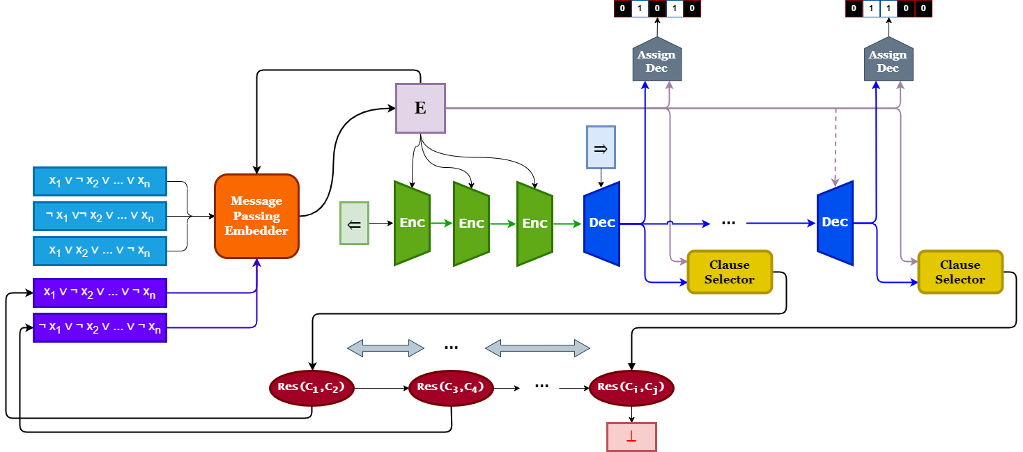
Figure 1: Overall NeuRes architecture

A CNF formula is satisfiable if there exists an assignment $\mathcal{A}:V\rightarrow\{\top,\bot\}$ such that all clauses are satisfied, i.e., each clause contains a positive literal $x$ such that $\mathcal{A}(x)=\top$ or a negative literal $\bar{x}$ such that $\mathcal{A}(x)=\bot$. If no such assignment exists we call the formula unsatisfiable. To prove unsatisfiability we rely on resolution, a fundamental inference rule in satisfiability testing (Davis & Putnam, 1960). The resolution rule (Res) picks clauses with two opposite literals and performs the following inference:

$$\prooftree\hypo{C_{1}\cup\{x\}}\hypo{C_{2}\cup\{\bar{x}\}}\infer 2[\textit{Res}]{C_{1}\cup C_{2}}$$

Resolution effectively performs a case distinction on the value of variable $x$: Either it is assigned to $\mathit{false}$, then $C_{1}$ has to evaluate to $\mathit{true}$, or it is assigned to $\mathit{true}$, then $C_{2}$ has to evaluate to $\mathit{true}$. Hence, we may infer the clause $C_{1}\cup C_{2}$. A resolution proof for a CNF formula is a sequence of applications of the Res rule ending in the empty clause.

4 Models

4.1 General Architecture

NeuRes is a neural network that takes a CNF formula as a set of clauses and outputs either a satisfying truth assignment or a resolution proof of unsatisfiability. As such, our model comprises a formula embedder followed by an LSTM-based encoder-decoder network connected to two downstream heads: (1) an attention network responsible for selecting clause pairs, and (2) a truth assignment decoder. See Figure 1 for an overview of the NeuRes architecture. After obtaining the initial clause and literal embeddings (representing the input formula), they are passed through the encoder to get the initial hidden state of the decoder, which marks the certificate generation phase. At each step, the model selects a clause pair which gets resolved into a new clause to append to the current formula graph while decoding a candidate truth assignment in parallel. The model keeps deriving new clauses until the empty clause is found (marking resolution proof completion), a satisfying assignment is found (marking a certified sat verdict), or the limit on episode length is reached (marking timeout).

4.2 Message-Passing Embedder

Similar to NeuroSAT, we use a message-passing GNN to obtain clause and literal embeddings by performing a predetermined number of rounds. Our formula graph is also constructed in a similar fashion to NeuroSAT graphs where clause nodes are connected to their constituent literal nodes and literals are connect to their complements (cf. Appendix A). For a formula $F$ in $m$ variables and $n$ clauses, the outputs of this GNN are two matrices: $E^{L}\in\mathbb{R}^{m\times d}$ for literal embeddings and $E^{C}\in\mathbb{R}^{{n}\times d}$ for clause embedding, where $d\in\mathbb{N^{+}}$ is the embedding vector width. Here we have two key differences from NeuroSAT. Firstly, NeuroSAT uses these embeddings as voters to predict satisfiability through a classification MLP. In our case, we use these embeddings as clause tokens for clause pair selection and literal tokens for truth value assignment. Secondly, since our model derives new clauses with every resolution step, we need to embed these new clauses, as well as update existing embeddings to reflect their relation to the newly inferred clauses. Consequently, we need to introduce a new phase to the message-passing protocol, for which we explore two approaches: static embeddings and dynamic embeddings.

In a static approach, we do not change the embeddings of initial clauses upon inferring a new clause. Instead, we exchange local messages between the node corresponding to the new clause and its literal nodes, in both directions. The main advantage of this approach is its low cost. A major drawback is that initial clauses never learn information about their relation to newly inferred clauses.

In a dynamic approach, we do not only generate a new clause and its embedding, we also update the embeddings of all other clauses. This accounts for the fact that the utility of an existing clause may change with the introduction of a new clause. We perform one message-passing round on the mature graph for every newly derived clause, which produces the new clause embedding and updates other clause embeddings. Since message-passing rounds are parallel across clauses, a single update to the whole embedding matrix is reasonably efficient.

4.3 Selector Networks

After producing clause and literal embeddings followed by the encoder phase, NeuRes enters the derivation stage. At each step, our model needs to select two clauses to resolve, produce the resultant clause, and add it to the current formula. We tokenize clauses by their embeddings as opposed to their encoder outputs as in a Pointer Network. The reason for that is that our embeddings are dynamic, and so the encoder outputs need to be dynamic, too. While embeddings can be updated in parallel, encoder outputs are generated in sequence, which is costly.

To realize our clause-pair selection mechanism, we employ three attention-based designs. With the decoder as the main driver for our model, at each step $t$ we use the decoder hidden state vector $h_{t}$ for querying our attention networks over the set of tokens (clauses or literals).

4.3.1 Cascaded Pointer-Attention (Casc-Attn)

In this design, pairs are selected by making two consecutive attention queries on the clause pool. We condition the second attention query on the outcome (i.e., the clause) of the first query. Figure 2 shows this scheme where we perform the first query using $h_{t}$ concatenated with a zero token vector while performing the second query using $h_{t}$ concatenated with the embedding vector $E^{C}_{i}$ of the clause selected in the first query.

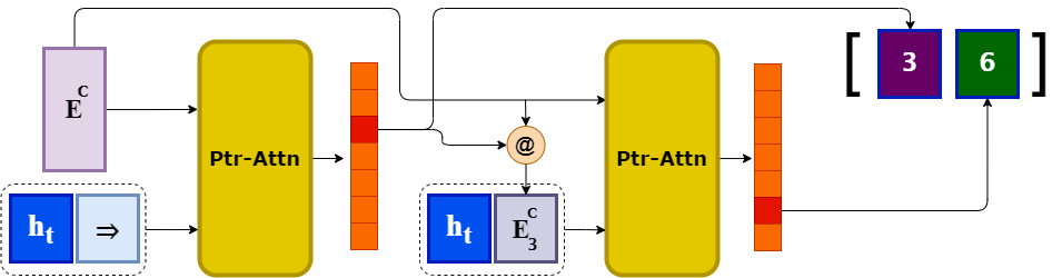
Figure 2: Cascaded Attention

Formally, Casc-Attn selects a clause index pair $(c_{1},c_{2})$ as follows:

$$c_{r}=\operatorname*{\textbf{argmax}}_{i}\left[u^{T}\tanh(W_{1}Q_{r}+W_{2}E^{C}_{i})\right]$$ (2)

where $W_{1}\in\mathbb{R}^{2d\times d},W_{2}\in\mathbb{R}^{d\times d},u\in\mathbb{R}^{d}$ are trainable network parameters.

The advantage of this design is that it is not limited to pair selection and can be used to select a tuple of arbitrary length. The main downside, however, is that this design chooses $c_{1}$ independently from $c_{2}$, which is undesirable because the utility of a resolution step is determined by both clauses simultaneously (not sequentially).

4.3.2 Full Self-Attention (Full-Attn)

To address the downside of independent clause selection, this variant performs self-attention between all clauses to obtain a matrix $S\in\mathbb{R}^{n\times n}$ where $S_{i,j}$ represents the attention score of the clause pair $(C_{i},C_{j})$ as shown in Figure 3. The model selects clause pairs by choosing the cell with the maximal score. In this attention scheme, clause embeddings are used as keys while queries are constructed by concatenating the decoder hidden state $h_{t}$ with all clause embeddings.

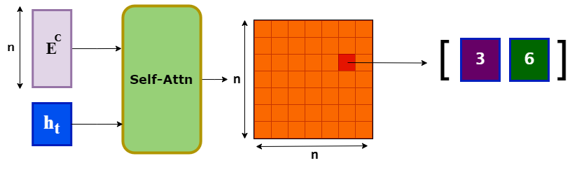
Figure 3: Full Self-Attention

Formally, Full-Attn selects a clause index pair $(c_{1},c_{2})$ as follows:

$$(c_{1},c_{2})=\operatorname*{\textbf{argmax}}_{(i,j)}\,\,S_{i,j}$$ (3)

where $W_{Q}\in\mathbb{R}^{2d\times d},W_{K}\in\mathbb{R}^{d\times d}$ are trainable network parameters. Since $S$ contains many cells that correspond to invalid resolution steps (i.e., clause pairs that cannot be resolved), we mask out the invalid cells from the attention grid in ensure the network selection is valid at every step.

4.3.3 Anchored Self-Attention (Anch-Attn)

In Full-Attn, the attention grid grows quadratically with the number of clauses. In this variant, we relax this cost by exploiting a property of binary resolution where each step targets a single variable in the two resolvent clauses. This allows us to narrow down candidate clause pairs by first selecting a variable as an anchor on which our clauses should be resolved. As such, we do not need to consider the full clause set at once, only the clauses containing the chosen variable $v$. We further compress the attention grid by lining clauses containing the literal $v$ on rows while lining clauses containing the literal $\neg v$ on columns. This reduces the redundancy of the attention grid since clauses containing the variable $v$ with the same parity cannot be resolved on $v$, so there is no point in matching them. In the worst case, this relaxed grid is of size $\frac{n}{2}\times\frac{n}{2}=\frac{n^{2}}{4}$ instead of $n^{2}$. In this scheme, we have two attention modules: one pointer-attention network to choose an anchor variable followed by a self-attention network to produce the anchored score grid.

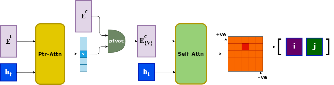
Figure 4: Anchored Self-Attention

In light of Figure 4, this approach combines structural elements from Casc-Attn (pointer attention) and Full-Attn (self-attention); however, both elements are used differently in Anch-Attn. Firstly, pointer-attention in Casc-Attn is used to select clauses whereas Anch-Attn uses it to select variables. Secondly, self-attention in Full-Attn matches any pair of clauses ($C_{i}$, $C_{j}$) in both directions as the row and column dimensions in the attention score grid reflect the same clauses (all clauses). By contrast, Anch-Attn computes self-attention scores for clause pairs in only one order (positive instance to negative instance). Formally, Anch-Attn selects an anchor variable $v$ as follows:

where $W_{1}\in\mathbb{R}^{d\times d},W_{2}\in\mathbb{R}^{d\times d},u\in\mathbb{R}^{d}$ are trainable network parameters. The clause index pair $(c_{1},c_{2})$ is then selected according to the same equations of Full-Attn (Eq. 3) using the $v$-anchored set of clause embeddings.

4.4 Assignment Decoder

To extract satisfying assignments, we condition literal embeddings $E^{L}$ on the decoder hidden state $h_{t}$ and then use a sigmoid-activated MLP $\psi$ to assign a truth value $\hat{\mathcal{A}}(l_{i})$ to a literal $l_{i}$ as shown in Eq. 5.

Note that since for each variable, we have a positive and a negative literal embeddings, we can construct two different truth assignments at a time using this method. However, to simplify our loss function, we only derive truth assignments from the positive literal embeddings at train time while extracting both at test time.

5 Training and Hyperparameters

5.1 Dataset

For our training and testing data, we adopt the same formula generation method as NeuroSAT, namely $\textbf{SR}(n)$ where $n$ is the number of variables in the formula. This method was designed to generate a generalized formula distribution that is not limited to a particular domain of SAT problems. To control our data distributions, we vary the range on the number of Boolean variables involved in each formula. For our training data, we use formulas in $\text{{SR}}(U(10,40))$ where $U(10,40)$ denotes the uniform distribution on integers between 10 and 40 (inclusive). To generate our teacher certificates comprising resolution proofs and truth assignments, we use the BooleForce solver (Biere, 2010) on the formulas generated on the SR distribution.

5.2 Loss Function

We train our model in a supervised fashion using teacher-forcing on solver certificates. During unsat episodes, teacher actions (clause pairs) are imposed over the whole run. The length of the teacher proof dictates the length of the respective episode, denoted as $T$. Model parameters $\theta$ are trained to maximize the likelihood of teacher choices $y_{t}$ thereby minimizing the resolution loss $\mathcal{L}_{Res}$ shown in Eq 6.

$$\begin{split}\mathcal{L}_{Res}=-\frac{1}{T}\sum_{t}{\log(p(y_{t};\theta))}\cdot\gamma^{(T-t)}\end{split}$$ (6)

During sat episodes, we minimize $\mathcal{L}_{sat}$ computed as the binary cross-entropy loss between the sigmoid-activated outputs of assignment decoder $\hat{\mathcal{A}}:V\rightarrow[0,1]$ and the teacher assignment $\mathcal{A}:V\rightarrow\{0,1\}$ as shown in Eq. 7.

$$\begin{split}\scalebox{0.95}{$\mathcal{L}_{sat}=\frac{1}{T}\sum\limits_{t}\left[\frac{\gamma^{(T-t)}}{|V|}{\sum\limits_{v}^{V}\text{BCE}(\hat{\mathcal{A}}(v),\mathcal{A}(v))}\right]$}\end{split}$$ (7)

In both types of episodes, step-wise losses are weighted by a time-horizon discounting factor $\gamma<1.0$ over the whole episode. The main rationale behind this is that later losses should have higher weights as the formula tends to get easier to solve with each new clause inferred by resolution.

5.3 Hyperparameters

Our neural solver has several hyperparameters that influence network size, depth, and loss weighting. Embedding and hidden state vectors have a fixed width of 512. We train our model with a batch size of 1 and the Adam optimizer (Kingma & Ba, 2014) for 50 epochs. We linearly anneal the learning rate from $5\times 10^{-5}$ to zero over the training episodes. This yields better results than using a constant learning rate (cf. Appendix E). We use a time discounting factor $\lambda=0.99$ for the episodic loss. We apply global-norm gradient clipping with a ratio of 0.5 (Pascanu et al., 2012).

6 Generating Resolution Proofs

NeuRes uses resolution as the core reasoning technique for certificate generation, both in the unsat and sat cases. Hence, we start with an in-depth comparative evaluation of several internal variants for resolution only. In particular, we evaluate the success rate (i.e., problems solved before timeout) and proof length relative to teacher, denoted as $\text{p-Len}=\frac{|\mathcal{P}_{\text{NeuRes}}|}{|\mathcal{P}_{\text{teacher}}|}$. We use a limit of $4$ on this ratio as a timeout to avoid simply brute-forcing a resolution proof. Note that we measure p-Len only for solved formulas to avoid diluting the average with resolution trails that timed out. For our evaluation, overall problem difficulty is quantified by the number of variables involved in the formula. For experiments in this section, we train on 8K unsat formulas in $\text{{SR}}(U(10,40))$ and test our models on 10K unseen formulas belonging to the same distribution. We use more formulas than the model was trained on to more reliably demonstrate its learning capacity.

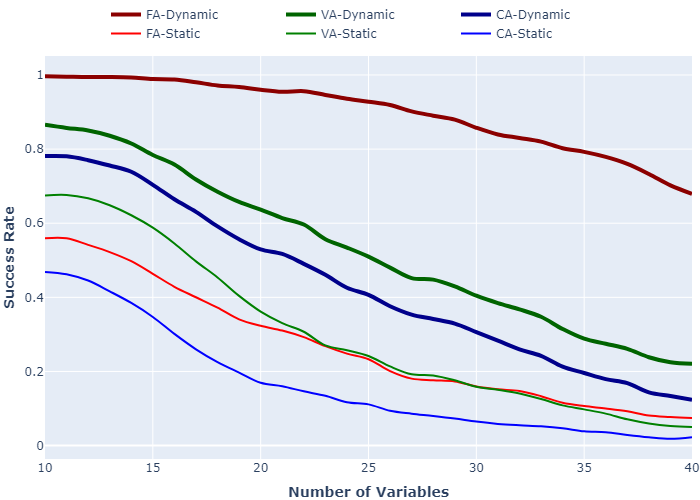
Figure 5: Performance of all attention variants for unsat problems with different numbers of variables.

6.1 Attention Variants

To assess the basic resolution performance of NeuRes, we evaluate each attention variant using both static and dynamic embeddings. For this experiment, we perform 32 rounds of message-passing for each input formula.

Table 1: Performance of all attention variants on $\text{{SR}}(U(10,40))$ unsat test formulas.

Variant	Static-Embed		Dynamic-Embed
	Solved (%)	p-Len	Solved (%)	p-Len
Casc-Attn	13.62	1.8	38.98	1.97
Full-Attn	23.68	1.59	87.19	1.74
Anch-Attn	26.28	1.99	48.63	1.6

As shown in Table 1, dynamic embedding is decisively better for all three attention variants, thereby confirming its conceptual merit. While Anchored-Attention leads over other variants under static embeddings, Full-Attention performs significantly better for dynamic embeddings, albeit at the cost of longer proofs on average. We believe that Anch-Attn’s better performance in the static setting can be explained through the full connectivity of its attention grid (proven in Appendix B).

On a closer look, Full-Attn particularly leads the field on difficult formulas that contain more variables. Figure 5 illustrates the performance of the variants for formulas in different numbers of variables. All variants exhibit a nearly monotonic inverse proportionality between the number of variables and the success rate. However, the decline happens at a much slower rate for dynamic Full-Attn than for other variants.

Since dynamic-embedding Full-Attn is the best-performing configuration over in-distribution test settings, we will demonstrate the remaining evaluation experiments exclusively on this variant.

6.2 Number of Message-Passing Rounds

The number of message-passing rounds is an important parameter for the model performance. We experiment with a fixed-length protocol (16, 32, 64), and an adaptive protocol that performs $|V|+1$ rounds to adapt to problem size. This number corresponds to the maximum formula graph diameter (i.e., $|V|+1$) and, hence, guarantees full exploration of graph connections at the end of the protocol. Performance results shown in Table 2 confirm that the adaptive protocol performs significantly better than fixed-length variants. Also, we see that performing too many rounds is in fact detrimental to overall performance, as the success rate drops sharply when more rounds (64) than the number of variables (10 – 40) are performed.

Table 2: Performance for different numbers of message-passing rounds on $\text{{SR}}(U(10,40))$ unsat test formulas.

#Rounds	Solved (%)	p-Len
16	82.12	1.83
32	87.19	1.74
64	52.11	1.77
$|V|+1$	89.43	1.71

This finding is of practical significance because it removes the need for optimizing the protocol length as a hyperparamter for a given dataset distribution, which sets NeuRes apart from related approaches such as NeuroSAT. All subsequent experiments exclusively use this adaptive variant.

Table 3: Bootstrapped training data reduction statistics. Gen-2 and Gen-3 metrics are computed relative to their predecessor-shrunk dataset. Gen-1 and Overall are evaluated relative to the original training dataset. Reduction stats are computed on an $\text{{SR}}(U(10,40))$ training dataset while p-Len and success rate are computed on a test set of the same distribution.

	Gen-1	Gen-2	Gen-3	Overall
Reduction Depth (max, avg)	$(9,2.53)$	$(8,1.59)$	$(5,1.48)$	$(13,2.55)$
Proofs Reduced (%)	57.49	43.12	37.77	75.84
Proof Reduction (max, avg) (%)	(86.11, 28.31)	(59.78, 12.99)	(58.23, 10.74)	(86.11, 31.81)
Total Reduction (%)	13.92	5.54	4.57	22.41
p-Len	1.505	1.367	1.23	1.23
Success Rate (%)	76.87	88.27	92.84	92.84

6.3 Shortening Teacher Proofs with Bootstrapping

During our initial experiments, we discovered proofs produced by NeuRes that were shorter than the corresponding teacher proofs in the training data. Although teacher proofs were generated by a traditional SAT solver, they are not guaranteed to be size-optimal. The size of resolution proofs is their only real drawback, hence any method that can reduce this size would be immensely useful. Upon closer inspection we find that, on average, our previous best performer trained with regular teacher-forcing manages to shorten $\sim$$18\%$ of teacher proofs by a notable factor (cf. Appendix D).

This inspired us to devise a bootstrapped training procedure to capitalize on this feature: We pre-roll each input problem using model actions only, and whenever the model proof is shorter than the teacher’s, it replaces the teacher’s in the dataset. In other words, we maximize the likelihood of the shorter proof. In doing so iteratively, the model progressively becomes its own teacher by exploiting redundancies in the teacher algorithm. This introduces a bias towards the model’s own actions while reducing variance by having a more concise learning signal in form of shorter proofs. To mitigate this bias effect, we train several model generations, each trained on the reduced data pool of its predecessor. Each fresh model gets trained on proofs shortened by a different model, which allows the later generations to both exploit the existing reduction insights without having an encoded bias towards them. In the case of a single generation, the latter effect gets throttled, as the model matures, due to that self-bias, which gets reset in each new generation.

The outcome of this bootstrapped training process is summarized in Table 3, where Gen-1 is the model in the first bootstrapping generation. As we can see, the models success rate initially declines compared to the original variant without proof shortening (cf. Table 1). We believe that the shortening entails the model specializing in a subset of the training formulas at the expense of limiting the model’s generality. While this enhances quality of the proofs (on some formulas), it limits the quantity of proofs, i.e., of solved instances. Nevertheless, we find that the performance loss from bootstrapping is gradually overcome through Gen-2 and Gen-3 until eventually beating the non-bootstrapped baseline in terms of both success rate and optimality by a notable margin. The sharp decline in proof length at test time (p-Len) shows that the models transfers the bootstrapped knowledge to unseen test formulas, as opposed to just overfitting on training formulas. In addition to success rate and p-Len, we inspect the reduction statistics of our bootstrapped generations (first three rows of Table 3). Since Gen-x models perform multiple reduction scans over the training dataset, we add a metric of reduction depth computed as the number of progressive reductions made to a proof. To further quantify this effect, we report the maximum and average reduction ratios of reduced proofs relative to teacher proofs. Finally, we report the total reduction made to the dataset size in terms of total proof steps.

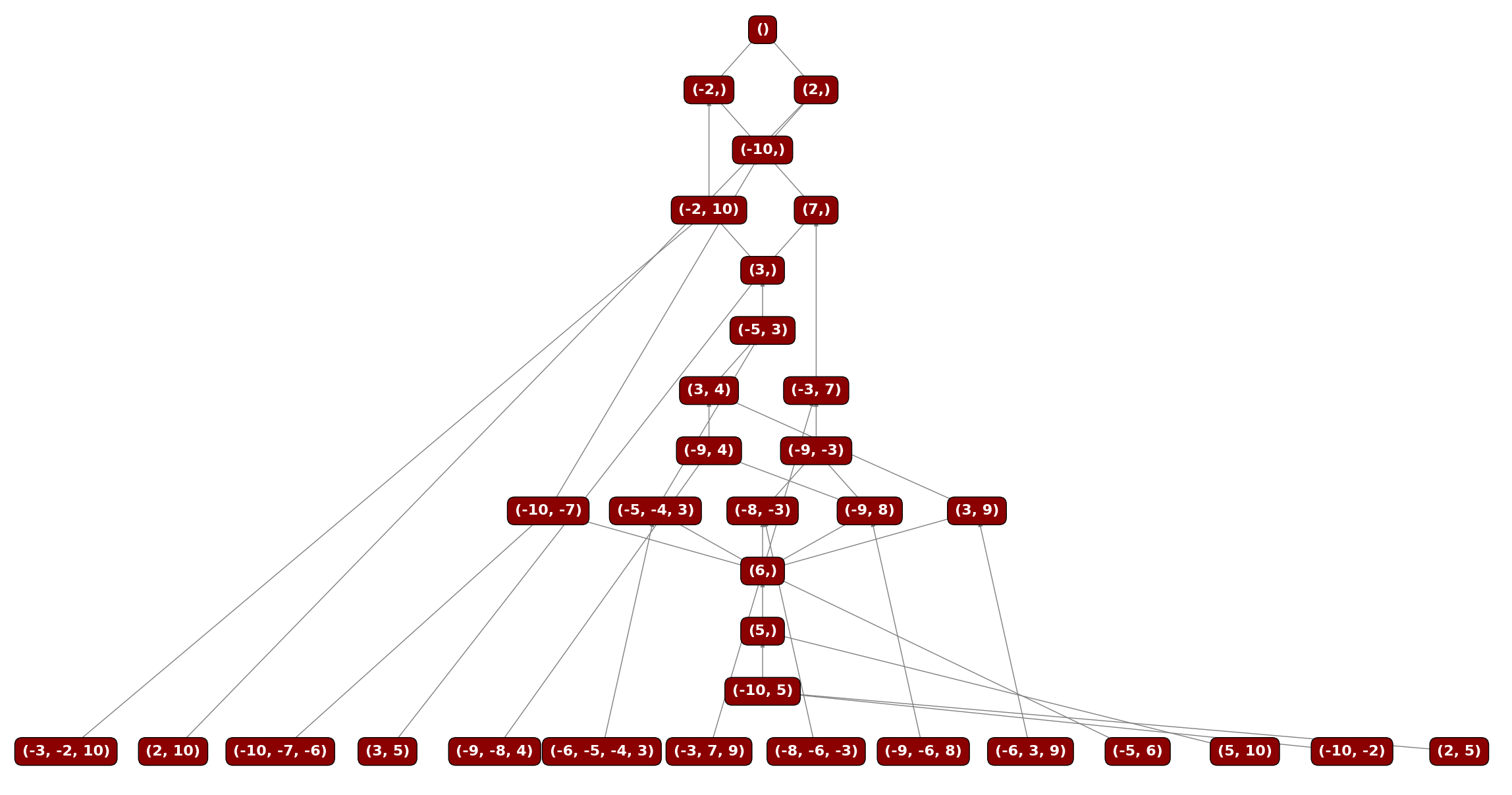
(a) Teacher Proof

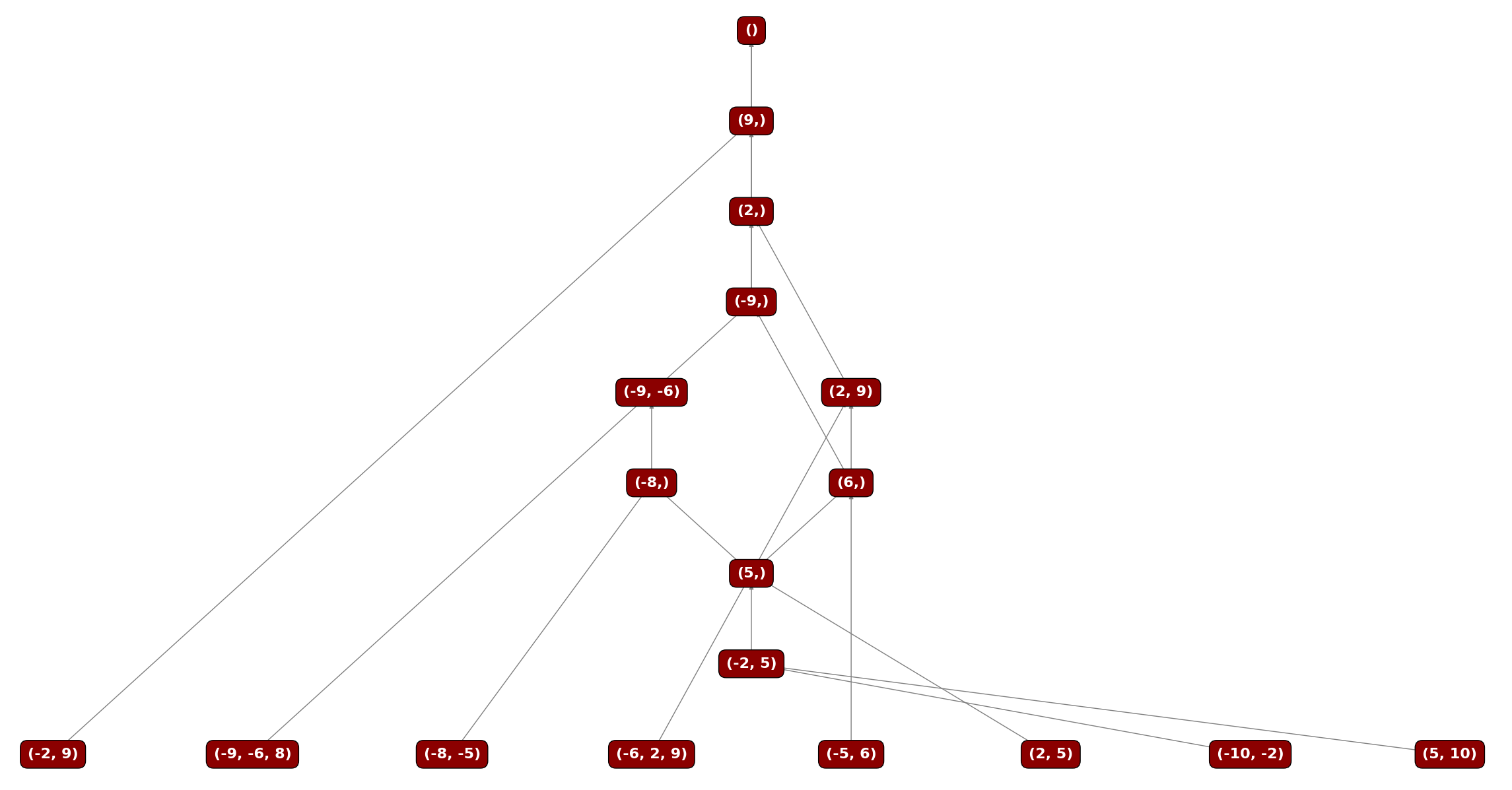
(b) NeuRes Proof

Figure 10: Teacher Proof Reduction Example

In Appendix D, we have compiled additional statistics (cf. Table 5 and Figure 9) on proof shortening during the training process, as well as an example proof reduced by the bootstrapped NeuRes (Figure 10). We only include a small reduction example (from 20 steps to 10 steps) for space constraints, but we have many more examples of much larger reductions (e.g., from $\sim$$800$ to $\sim$$400$ steps).

Table 4: Performance of different full solver modes on $\textbf{SR}(40)$. All models were trained on the $\text{{SR}}(U(10,40))$ distribution.

Solver	Sat		Unsat		Total
	Solved (%)	#Iterations	Solved (%)	p-Len	Solved (%)
Res-Aided	94.4	8.62	70.8	1.33	82.6
Res-Detached	90.2	6.64	67.0	1.5	78.6
NeuroSAT	70	-	-	-	-

7 Resolution-Aided SAT Solving

In this section, we evaluate the performance of the full integrated SAT solver trained on a hybrid dataset comprising 8K unsatisfiable formulas (and their resolution proofs) and 8K satisfiable formulas (and their satisfying assignments). For the former, timeout ($4\cdot{|\mathcal{P}_{\text{teacher}}|}$) and optimality (p-Len) are measured similarly to previous experiments. For satisfiable formulas, we set the timeout (maximum #trials) to $2\cdot|V|$. In this section, we verify that coupling resolution with sat assignment decoding boosts the overall success rate, by evaluating NeuRes in two functional modes that differ only in how they process sat formulas:

• Res-Detached: Decodes sat assignments on the original formula with no resolution guidance.

• Res-Aided: Decodes sat assignments on formulas augmented by resolution-derived clauses.

Table 4 points to three main takeaways. We see that the Res-Aided variant exhibits a higher sat performance than Res-Detached which only considers sat assignments on original clauses. This confirms the merit of augmenting formulas with resolution derivations in accelerating the process of finding satisfying assignments. We also observe a gain in unsat performance for Res-Aided. A potential explanation for this effect could be that skipping resolution during sat episodes induces a misalignment between the shared representations (e.g., embeddings and decoder hidden states) and the resolution network. Lastly, we compare the NeuRes performance on $\textbf{SR}(40)$ to that of NeuroSAT’s. Note that we can only compare the with NeuroSAT in terms of the percentage of sat problems solved, not merely correctly classified. This is because the former is backed with an easy-to-check SAT assignment while the latter is only a single-bit prediction that would require solving the whole problem to verify – making it far less useful. Moreover, there is no unsat success rate for NeuroSAT as it does not produce certificates for unsatisfiability (only predictions). As Table 4 shows, all three NeuRes variants outperform NeuroSAT, with Res-Aided in particular having a remarkably higher sat success rate when trained on the same $\text{{SR}}(U(10,40))$ distribution. This is doubly promising considering NeuroSAT was trained on millions of formulas while NeuRes was trained on only 16K formulas.

7.1 Generalizing to Larger Problems

We also evaluate our Res-Aided model (trained on $\text{{SR}}(U(10,40))$) on five datasets comprising formulas with up to 5 times more variables than encountered during training. We use the same distributions reported by NeuroSAT and we run our model for the same maximum number of iterations (1000).

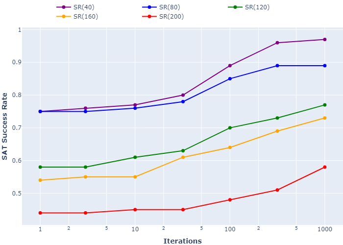
Figure 6: SAT success rate over iterations.

For this experiment, instead of performing the maximum-score resolution step, we pool the top 50 steps and perform the one that results in the shortest clause. This was found to bring considerable gains to the success rate on larger formula distributions. In Appendix F, we show the base performance obtained without this optimization.

Figure 6 shows the scalability of NeuRes to larger problems by letting it run for more iterations. Compared to NeuroSAT (cf. Selsam et al. (2019)), NeuRes scores a much higher first-try success rate on all 5 problem distributions, and a higher final success rate on all of them except for $\textbf{SR}(40)$ and $\textbf{SR}(40)$ on which our performance is very close to NeuroSAT’s. Particularly, NeuRes shows an adequate first-try success on the 3 largest problem sizes where NeuroSAT solves zero or near-zero problems on the first try.

8 Conclusion

In this paper, we have presented NeuRes, the first proof-generating neuro-symbolic SAT solver. Unlike other neural SAT solvers in the literature, NeuRes is sound-by-design; therefore it does not need an auxiliary SAT solver to validate its verdicts or certificates. Structurally, NeuRes is a fusion between Pointer Networks and NeuroSAT that advances the functional capabilities of both of them. On the one hand, it extends Pointer Networks by not only generating solutions composed of input tokens but also combinations of a growing pool thereof. On the other hand, NeuRes far surpasses NeuroSAT in terms of performance and data efficiency owing to its resolution-aided mode of operation and certificate-based training process. Moreover, unlike NeuroSAT, NeuRes is a full solver rather than a mere classifier.

Despite its promising benchmark performance, NeuRes cannot solely outperform highly-engineered industrial solvers, as is the case for all neuro-symbolic methods as standalone tools. Nevertheless, NeuRes has demonstrated a unique potential to advance SAT solving through its ability of proof reduction, as proof size is a major challenge in certifying the results of traditional solvers. NeuRes proof reduction is facilitated by a bootstrapped training procedure that uses teacher proofs as a guide as opposed to a golden standard. This relaxation of supervision, together with NeuRes’ data efficiency, naturally points to future work on unsupervised neuro-symbolic methods.

9 Impact Statement

This paper presents work whose goal is to advance the fields of Machine Learning and SAT Solving. There are many potential societal consequences of our work, none of which we feel must be specifically highlighted here.

Appendix A NeuroSAT Formula Graph Construction

(a) Literal-to-Clause Phase

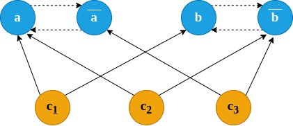
(b) Clause-to-Literal Phase

Figure 7: Two-phase message-passing round on NeuroSAT formula graph.

NeuroSAT-style formula graphs have two designated node types: clause nodes connected to the literal nodes corresponding to their constituent literals (Selsam et al., 2019). For example, in Figure 7, the clause contents are as follows: $c_{1}=(a\lor b),\quad c_{2}=(a\lor\bar{b}),\quad c_{3}=(\bar{a}\lor\bar{b})$. Each message-passing round involves two exchange phases: (1) Literal-to-Clause, and (2) Clause-to-Literal (and implicitly Literal-to-Complement). This construction is particularly efficient as it allows the message-passing protocol to cover the entire graph connectivity in at most $|V|+1$ rounds where $V$ is the set of variables in the formula.

Appendix B Clause Connectivity Under Static Embeddings

In Section 4.2, we stated that under static embeddings for a derived clause, as the embedder creates its embedding, it only updates the representations of the variables involved in it – leaving other clause embeddings intact. This might present a problem for Full-Attn where the attention grid contains all clauses including disconnected pairs. An example of such a pair would be two derived clauses that do not share a variable. This could potentially lower the efficacy of the Full-Attn mechanism as it tries to match clauses that are unaware of each other. Interestingly, despite being a relaxation on Full-Attn, Anch-Attn has a distinct edge over Full-Attn under static embeddings in form of the following property:

Lemma B.1.

Clauses in the variable-anchored attention grid of Anch-Attn are guaranteed to be connected under both static and dynamic embeddings.

Proof.

Let $v$ be a variable in the input formula, and the set of clauses of a $v$-anchored attention grid be $A$. We show that we always have at least one clause $A_{i}\in A$ that reaches all other clauses in $A$ on the formula graph. We make two case distinctions:

Case 1: All clauses in $A$ are input clauses (in the original formula). Here, the lemma follows trivially since all these clause were connected during the input-phase message-passing protocol as they share at least one variable $v$.

Case 2: $A$ contains derived clauses. Let $A_{i}$ be the most recently derived clause in $A$. Since $A_{i}$ shares variable $v$ with all other clauses in $A$, then $A_{i}$ would be connected to them all during the derivation-phase message-passing protocol immediately after $A_{i}$ was derived. This is because $A_{i}$ receives a message from $V$ (under both static and dynamic embeddings) containing information about all other clauses containing $v$, which is precisely $A\setminus\{A_{i}\}$. Therefore, the lemma holds. ∎

Appendix C Further unsat Performance Breakdowns

(a) Success Rate vs. #Variables

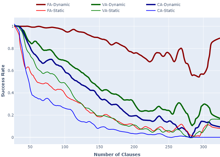
(b) Success Rate vs. #Clauses

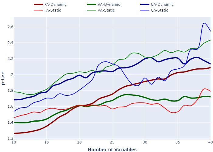
(c) p-Len vs. #Variables

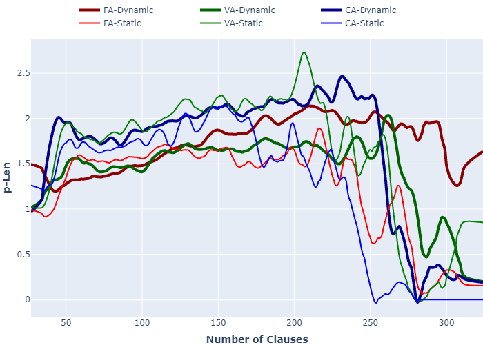
(d) p-Len vs. #Clauses

Figure 8: Performance of all attention variants on $\text{{SR}}(U(10,40))$ unsat test formulas. All models were trained on 8K $\text{{SR}}(U(10,40))$ formulas.

Appendix D Teacher Proof Reduction

Table 5: Teacher proof reduction statistics of non-bootstrapped model trained on unreduced $\text{{SR}}(U(10,40))$ dataset. Note that all rows, except for Total Reduction, are computed over the reduced portion of the dataset, i.e., the proofs that were successfully shortened by NeuRes.

(%)	Train	Test
Proofs Reduced	17.82	18.29
Max. Reduction	86.11	76.4
Avg. Reduction	23.55	23.65
Total Reduction	3.07	3.15

On rather interesting observation on Table 5 is that the model appears to be marginally better at producing shorter proofs for unseen (test) formulas than for training formulas. While we would normally expect the opposite, a fair speculation would be that the trained model was teacher-forced to match teacher proofs during training over multiple epochs while the same does not hold for unseen formulas where the bias towards teacher behavior is significantly lower. To definitively confirm this would require a more in-depth investigation.

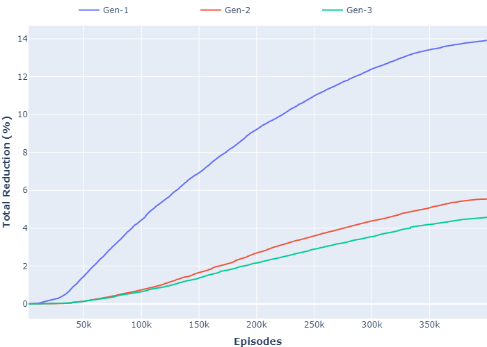
Figure 9: The progression of the total reduction made by each generation to their given training dataset. We observe that Gen-1 has the highest slope as it operated on the original unreduced dataset whereas Gen-2 and Gen-3 operated on already-reduced datasets where there is less room for further reductions.

Figure 9 shows the progression of the total reduction made by each generation to their given training dataset. We observe that Gen-1 has the highest slope as it operated on the original unreduced dataset whereas Gen-2 and Gen-3 operated on already-reduced datasets where there is less room for further reductions. Indeed, we already see that effect in miniature for all three progressions as their slope tends to attenuate near the end.

Appendix E Constant vs. Linearly Annealed Learning Rate

Here we show the effect of linearly annealing the Adam optimizer base learning rate to zero over the number of training episodes on the validation success rate throughout training. As shown in Figure 11, linear annealing brings considerable gains to the model performance. Consequently, we use a linearly annealed learning rate for all our main experiments.

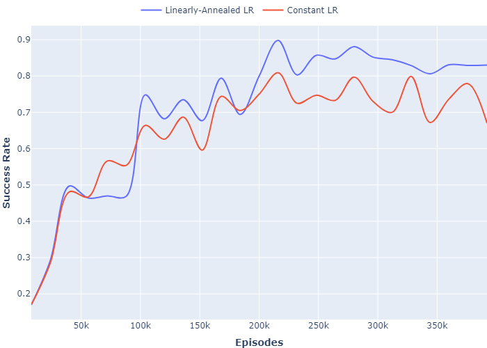
Figure 11: Validation Success Rate With Different LR Schedules

Appendix F Out-Of-Distribution Performance

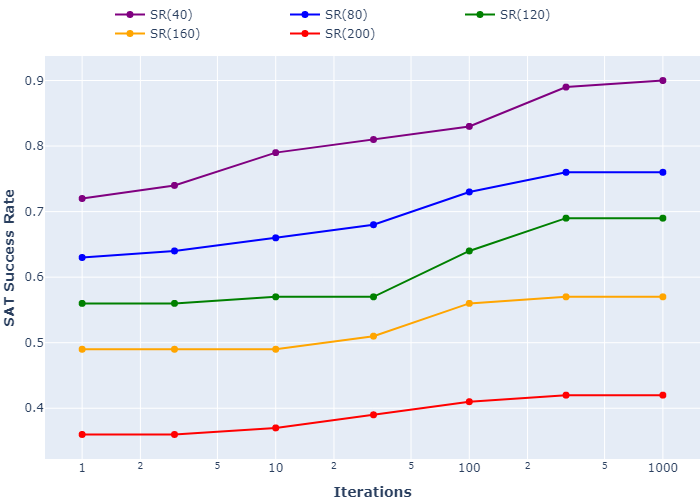
Figure 12: sat success rate over iterations using base Res-Aided NeuRes

References

- Amizadeh et al. (2019) Amizadeh, S., Matusevych, S., and Weimer, M. Learning to solve circuit-sat: An unsupervised differentiable approach. In 7th International Conference on Learning Representations, ICLR 2019, New Orleans, LA, USA, May 6-9, 2019. OpenReview.net, 2019. URL https://openreview.net/forum?id=BJxgz2R9t7.
- Balint et al. (2013) Balint, A., Belov, A., Heule, M., and Järvisalo, M. (eds.). Proceedings of SAT Competition 2013: Solver and Benchmark Descriptions, volume B-2013-1 of Department of Computer Science Series of Publications B. University of Helsinki, Finland, 2013.
- Balunovic et al. (2018) Balunovic, M., Bielik, P., and Vechev, M. T. Learning to solve SMT formulas. In Bengio, S., Wallach, H. M., Larochelle, H., Grauman, K., Cesa-Bianchi, N., and Garnett, R. (eds.), Advances in Neural Information Processing Systems 31: Annual Conference on Neural Information Processing Systems 2018, NeurIPS 2018, December 3-8, 2018, Montréal, Canada, pp. 10338–10349, 2018. URL https://proceedings.neurips.cc/paper/2018/hash/68331ff0427b551b68e911eebe35233b-Abstract.html.
- Balyo et al. (2023) Balyo, T., Heule, M., Iser, M., Järvisalo, M., and Suda, M. (eds.). Proceedings of SAT Competition 2023: Solver, Benchmark and Proof Checker Descriptions. Department of Computer Science Series of Publications B. Department of Computer Science, University of Helsinki, Finland, 2023.
- Bansal et al. (2019) Bansal, K., Loos, S. M., Rabe, M. N., Szegedy, C., and Wilcox, S. Holist: An environment for machine learning of higher order logic theorem proving. In Chaudhuri, K. and Salakhutdinov, R. (eds.), Proceedings of the 36th International Conference on Machine Learning, ICML 2019, 9-15 June 2019, Long Beach, California, USA, volume 97 of Proceedings of Machine Learning Research, pp. 454–463. PMLR, 2019. URL http://proceedings.mlr.press/v97/bansal19a.html.
- Bello et al. (2017) Bello, I., Pham, H., Le, Q. V., Norouzi, M., and Bengio, S. Neural combinatorial optimization with reinforcement learning. In 5th International Conference on Learning Representations, ICLR 2017, Toulon, France, April 24-26, 2017, Workshop Track Proceedings. OpenReview.net, 2017. URL https://openreview.net/forum?id=Bk9mxlSFx.
- Biere (2010) Biere, A. Booleforce sat solver. https://fmv.jku.at/booleforce/, 2010.
- Brummayer et al. (2010) Brummayer, R., Lonsing, F., and Biere, A. Automated testing and debugging of SAT and QBF solvers. In Strichman, O. and Szeider, S. (eds.), Theory and Applications of Satisfiability Testing - SAT 2010, 13th International Conference, SAT 2010, Edinburgh, UK, July 11-14, 2010. Proceedings, volume 6175 of Lecture Notes in Computer Science, pp. 44–57. Springer, 2010. doi: 10.1007/978-3-642-14186-7“˙6. URL https://doi.org/10.1007/978-3-642-14186-7_6.
- Cameron et al. (2020) Cameron, C., Chen, R., Hartford, J. S., and Leyton-Brown, K. Predicting propositional satisfiability via end-to-end learning. In The Thirty-Fourth AAAI Conference on Artificial Intelligence, AAAI 2020, The Thirty-Second Innovative Applications of Artificial Intelligence Conference, IAAI 2020, The Tenth AAAI Symposium on Educational Advances in Artificial Intelligence, EAAI 2020, New York, NY, USA, February 7-12, 2020, pp. 3324–3331. AAAI Press, 2020. doi: 10.1609/aaai.v34i04.5733. URL https://doi.org/10.1609/aaai.v34i04.5733.
- Cappart et al. (2023) Cappart, Q., Chételat, D., Khalil, E. B., Lodi, A., Morris, C., and Velickovic, P. Combinatorial optimization and reasoning with graph neural networks. J. Mach. Learn. Res., 24:130:1–130:61, 2023. URL http://jmlr.org/papers/v24/21-0449.html.
- Clarke et al. (2001) Clarke, E. M., Biere, A., Raimi, R., and Zhu, Y. Bounded model checking using satisfiability solving. Formal Methods Syst. Des., 19(1):7–34, 2001. doi: 10.1023/A:1011276507260. URL https://doi.org/10.1023/A:1011276507260.
- Cook (1971) Cook, S. A. The complexity of theorem-proving procedures. In Harrison, M. A., Banerji, R. B., and Ullman, J. D. (eds.), Proceedings of the 3rd Annual ACM Symposium on Theory of Computing, May 3-5, 1971, Shaker Heights, Ohio, USA, pp. 151–158. ACM, 1971. doi: 10.1145/800157.805047. URL https://doi.org/10.1145/800157.805047.
- Cosler et al. (2023) Cosler, M., Schmitt, F., Hahn, C., and Finkbeiner, B. Iterative circuit repair against formal specifications. In The Eleventh International Conference on Learning Representations, ICLR 2023, Kigali, Rwanda, May 1-5, 2023. OpenReview.net, 2023. URL https://openreview.net/pdf?id=SEcSahl0Ql.
- Darbari et al. (2010) Darbari, A., Fischer, B., and Marques-Silva, J. Industrial-strength certified SAT solving through verified SAT proof checking. In Cavalcanti, A., Déharbe, D., Gaudel, M., and Woodcock, J. (eds.), Theoretical Aspects of Computing - ICTAC 2010, 7th International Colloquium, Natal, Rio Grande do Norte, Brazil, September 1-3, 2010. Proceedings, volume 6255 of Lecture Notes in Computer Science, pp. 260–274. Springer, 2010. doi: 10.1007/978-3-642-14808-8“˙18. URL https://doi.org/10.1007/978-3-642-14808-8_18.
- Davis & Putnam (1960) Davis, M. and Putnam, H. A computing procedure for quantification theory. J. ACM, 7(3):201–215, 1960. doi: 10.1145/321033.321034. URL https://doi.org/10.1145/321033.321034.
- de Moura & Bjørner (2011) de Moura, L. M. and Bjørner, N. S. Satisfiability modulo theories: introduction and applications. Commun. ACM, 54(9):69–77, 2011. doi: 10.1145/1995376.1995394. URL https://doi.org/10.1145/1995376.1995394.
- First et al. (2023) First, E., Rabe, M. N., Ringer, T., and Brun, Y. Baldur: Whole-proof generation and repair with large language models. CoRR, abs/2303.04910, 2023. doi: 10.48550/arXiv.2303.04910. URL https://doi.org/10.48550/arXiv.2303.04910.
- Goldberg & Novikov (2003) Goldberg, E. I. and Novikov, Y. Verification of proofs of unsatisfiability for CNF formulas. In 2003 Design, Automation and Test in Europe Conference and Exposition (DATE 2003), 3-7 March 2003, Munich, Germany, pp. 10886–10891. IEEE Computer Society, 2003. doi: 10.1109/DATE.2003.10008. URL https://doi.ieeecomputersociety.org/10.1109/DATE.2003.10008.
- Hahn et al. (2021) Hahn, C., Schmitt, F., Kreber, J. U., Rabe, M. N., and Finkbeiner, B. Teaching temporal logics to neural networks. In 9th International Conference on Learning Representations, ICLR 2021, Virtual Event, Austria, May 3-7, 2021. OpenReview.net, 2021. URL https://openreview.net/forum?id=dOcQK-f4byz.
- Heule et al. (2014) Heule, M., Jr., W. A. H., and Wetzler, N. Bridging the gap between easy generation and efficient verification of unsatisfiability proofs. Softw. Test. Verification Reliab., 24(8):593–607, 2014. doi: 10.1002/stvr.1549. URL https://doi.org/10.1002/stvr.1549.
- Heule (2021) Heule, M. J. H. Proofs of unsatisfiability. In Biere, A., Heule, M., van Maaren, H., and Walsh, T. (eds.), Handbook of Satisfiability - Second Edition, volume 336 of Frontiers in Artificial Intelligence and Applications, pp. 635–668. IOS Press, 2021. doi: 10.3233/FAIA200998. URL https://doi.org/10.3233/FAIA200998.
- Heule & Kullmann (2017) Heule, M. J. H. and Kullmann, O. The science of brute force. Commun. ACM, 60(8):70–79, 2017. doi: 10.1145/3107239. URL https://doi.org/10.1145/3107239.
- Irving et al. (2016) Irving, G., Szegedy, C., Alemi, A. A., Eén, N., Chollet, F., and Urban, J. Deepmath - deep sequence models for premise selection. In Lee, D. D., Sugiyama, M., von Luxburg, U., Guyon, I., and Garnett, R. (eds.), Advances in Neural Information Processing Systems 29: Annual Conference on Neural Information Processing Systems 2016, December 5-10, 2016, Barcelona, Spain, pp. 2235–2243, 2016. URL https://proceedings.neurips.cc/paper/2016/hash/f197002b9a0853eca5e046d9ca4663d5-Abstract.html.
- Järvisalo et al. (2012) Järvisalo, M., Heule, M., and Biere, A. Inprocessing rules. In Gramlich, B., Miller, D., and Sattler, U. (eds.), Automated Reasoning - 6th International Joint Conference, IJCAR 2012, Manchester, UK, June 26-29, 2012. Proceedings, volume 7364 of Lecture Notes in Computer Science, pp. 355–370. Springer, 2012. doi: 10.1007/978-3-642-31365-3“˙28. URL https://doi.org/10.1007/978-3-642-31365-3_28.
- Kautz & Selman (1992) Kautz, H. A. and Selman, B. Planning as satisfiability. In Neumann, B. (ed.), 10th European Conference on Artificial Intelligence, ECAI 92, Vienna, Austria, August 3-7, 1992. Proceedings, pp. 359–363. John Wiley and Sons, 1992.
- Khalil et al. (2017) Khalil, E. B., Dai, H., Zhang, Y., Dilkina, B., and Song, L. Learning combinatorial optimization algorithms over graphs. In Guyon, I., von Luxburg, U., Bengio, S., Wallach, H. M., Fergus, R., Vishwanathan, S. V. N., and Garnett, R. (eds.), Advances in Neural Information Processing Systems 30: Annual Conference on Neural Information Processing Systems 2017, December 4-9, 2017, Long Beach, CA, USA, pp. 6348–6358, 2017. URL https://proceedings.neurips.cc/paper/2017/hash/d9896106ca98d3d05b8cbdf4fd8b13a1-Abstract.html.
- Kingma & Ba (2014) Kingma, D. P. and Ba, J. Adam: A method for stochastic optimization. arXiv preprint arXiv:1412.6980, 2014.
- Kool et al. (2019) Kool, W., van Hoof, H., and Welling, M. Attention, learn to solve routing problems! In 7th International Conference on Learning Representations, ICLR 2019, New Orleans, LA, USA, May 6-9, 2019. OpenReview.net, 2019. URL https://openreview.net/forum?id=ByxBFsRqYm.
- Lammich (2020) Lammich, P. Efficient verified (UN)SAT certificate checking. J. Autom. Reason., 64(3):513–532, 2020. doi: 10.1007/s10817-019-09525-z. URL https://doi.org/10.1007/s10817-019-09525-z.
- Lederman et al. (2020) Lederman, G., Rabe, M. N., Seshia, S., and Lee, E. A. Learning heuristics for quantified boolean formulas through reinforcement learning. In 8th International Conference on Learning Representations, ICLR 2020, Addis Ababa, Ethiopia, April 26-30, 2020. OpenReview.net, 2020. URL https://openreview.net/forum?id=BJluxREKDB.
- Marques-Silva et al. (2021) Marques-Silva, J., Lynce, I., and Malik, S. Conflict-driven clause learning SAT solvers. In Biere, A., Heule, M., van Maaren, H., and Walsh, T. (eds.), Handbook of Satisfiability - Second Edition, volume 336 of Frontiers in Artificial Intelligence and Applications, pp. 133–182. IOS Press, 2021. doi: 10.3233/FAIA200987. URL https://doi.org/10.3233/FAIA200987.
- Mikula et al. (2023) Mikula, M., Antoniak, S., Tworkowski, S., Jiang, A. Q., Zhou, J. P., Szegedy, C., Kucinski, L., Milos, P., and Wu, Y. Magnushammer: A transformer-based approach to premise selection. CoRR, abs/2303.04488, 2023. doi: 10.48550/ARXIV.2303.04488. URL https://doi.org/10.48550/arXiv.2303.04488.
- Ozolins et al. (2022) Ozolins, E., Freivalds, K., Draguns, A., Gaile, E., Zakovskis, R., and Kozlovics, S. Goal-aware neural SAT solver. In International Joint Conference on Neural Networks, IJCNN 2022, Padua, Italy, July 18-23, 2022, pp. 1–8. IEEE, 2022. doi: 10.1109/IJCNN55064.2022.9892733. URL https://doi.org/10.1109/IJCNN55064.2022.9892733.
- Paliwal et al. (2020) Paliwal, A., Loos, S. M., Rabe, M. N., Bansal, K., and Szegedy, C. Graph representations for higher-order logic and theorem proving. In The Thirty-Fourth AAAI Conference on Artificial Intelligence, AAAI 2020, The Thirty-Second Innovative Applications of Artificial Intelligence Conference, IAAI 2020, The Tenth AAAI Symposium on Educational Advances in Artificial Intelligence, EAAI 2020, New York, NY, USA, February 7-12, 2020, pp. 2967–2974. AAAI Press, 2020. doi: 10.1609/AAAI.V34I03.5689. URL https://doi.org/10.1609/aaai.v34i03.5689.
- Pascanu et al. (2012) Pascanu, R., Mikolov, T., and Bengio, Y. Understanding the exploding gradient problem. CoRR, abs/1211.5063, 2(417):1, 2012.
- Polu & Sutskever (2020) Polu, S. and Sutskever, I. Generative language modeling for automated theorem proving. CoRR, abs/2009.03393, 2020. URL https://arxiv.org/abs/2009.03393.
- Schmitt et al. (2021) Schmitt, F., Hahn, C., Rabe, M. N., and Finkbeiner, B. Neural circuit synthesis from specification patterns. In Ranzato, M., Beygelzimer, A., Dauphin, Y. N., Liang, P., and Vaughan, J. W. (eds.), Advances in Neural Information Processing Systems 34: Annual Conference on Neural Information Processing Systems 2021, NeurIPS 2021, December 6-14, 2021, virtual, pp. 15408–15420, 2021. URL https://proceedings.neurips.cc/paper/2021/hash/8230bea7d54bcdf99cdfe85cb07313d5-Abstract.html.
- Selsam & Bjørner (2019) Selsam, D. and Bjørner, N. S. Guiding high-performance SAT solvers with unsat-core predictions. In Janota, M. and Lynce, I. (eds.), Theory and Applications of Satisfiability Testing - SAT 2019 - 22nd International Conference, SAT 2019, Lisbon, Portugal, July 9-12, 2019, Proceedings, volume 11628 of Lecture Notes in Computer Science, pp. 336–353. Springer, 2019. doi: 10.1007/978-3-030-24258-9“˙24. URL https://doi.org/10.1007/978-3-030-24258-9_24.
- Selsam et al. (2019) Selsam, D., Lamm, M., Bünz, B., Liang, P., de Moura, L., and Dill, D. L. Learning a SAT solver from single-bit supervision. In 7th International Conference on Learning Representations, ICLR 2019, New Orleans, LA, USA, May 6-9, 2019. OpenReview.net, 2019. URL https://openreview.net/forum?id=HJMC_iA5tm.
- Sun et al. (2020) Sun, L., Gérault, D., Benamira, A., and Peyrin, T. Neurogift: Using a machine learning based sat solver for cryptanalysis. In Dolev, S., Kolesnikov, V., Lodha, S., and Weiss, G. (eds.), Cyber Security Cryptography and Machine Learning - Fourth International Symposium, CSCML 2020, Be’er Sheva, Israel, July 2-3, 2020, Proceedings, volume 12161 of Lecture Notes in Computer Science, pp. 62–84. Springer, 2020. doi: 10.1007/978-3-030-49785-9“˙5. URL https://doi.org/10.1007/978-3-030-49785-9_5.
- Tseitin (1983) Tseitin, G. S. On the complexity of derivation in propositional calculus. Automation of reasoning: 2: Classical papers on computational logic 1967–1970, pp. 466–483, 1983.
- Vinyals et al. (2015) Vinyals, O., Fortunato, M., and Jaitly, N. Pointer networks. Advances in neural information processing systems, 28, 2015.
- Vizel et al. (2015) Vizel, Y., Weissenbacher, G., and Malik, S. Boolean satisfiability solvers and their applications in model checking. Proc. IEEE, 103(11):2021–2035, 2015. doi: 10.1109/JPROC.2015.2455034. URL https://doi.org/10.1109/JPROC.2015.2455034.
- Wang et al. (2017) Wang, M., Tang, Y., Wang, J., and Deng, J. Premise selection for theorem proving by deep graph embedding. In Guyon, I., von Luxburg, U., Bengio, S., Wallach, H. M., Fergus, R., Vishwanathan, S. V. N., and Garnett, R. (eds.), Advances in Neural Information Processing Systems 30: Annual Conference on Neural Information Processing Systems 2017, December 4-9, 2017, Long Beach, CA, USA, pp. 2786–2796, 2017. URL https://proceedings.neurips.cc/paper/2017/hash/18d10dc6e666eab6de9215ae5b3d54df-Abstract.html.
- Wetzler et al. (2014) Wetzler, N., Heule, M., and Jr., W. A. H. Drat-trim: Efficient checking and trimming using expressive clausal proofs. In Sinz, C. and Egly, U. (eds.), Theory and Applications of Satisfiability Testing - SAT 2014 - 17th International Conference, Held as Part of the Vienna Summer of Logic, VSL 2014, Vienna, Austria, July 14-17, 2014. Proceedings, volume 8561 of Lecture Notes in Computer Science, pp. 422–429. Springer, 2014. doi: 10.1007/978-3-319-09284-3“˙31. URL https://doi.org/10.1007/978-3-319-09284-3_31.
- Yang & Deng (2019) Yang, K. and Deng, J. Learning to prove theorems via interacting with proof assistants. In Chaudhuri, K. and Salakhutdinov, R. (eds.), Proceedings of the 36th International Conference on Machine Learning, ICML 2019, 9-15 June 2019, Long Beach, California, USA, volume 97 of Proceedings of Machine Learning Research, pp. 6984–6994. PMLR, 2019. URL http://proceedings.mlr.press/v97/yang19a.html.
- Zhang & Malik (2003) Zhang, L. and Malik, S. Validating SAT solvers using an independent resolution-based checker: Practical implementations and other applications. In 2003 Design, Automation and Test in Europe Conference and Exposition (DATE 2003), 3-7 March 2003, Munich, Germany, pp. 10880–10885. IEEE Computer Society, 2003. doi: 10.1109/DATE.2003.10014. URL https://doi.ieeecomputersociety.org/10.1109/DATE.2003.10014.