Riemann–Hilbert method to the Ablowitz–Ladik equation: higher-order case

Abstract

We focused on the Ablowitz–Ladik equation on a zero background, specifically considering the scenario of $N$ pairs of multiple poles. Our first goal was to establish a mapping between the initial data and the scattering data. This allowed us to introduce a direct problem by analyzing the discrete spectrum associated with $N$ pairs of higher-order zeros. Next, we constructed another mapping from the scattering data to a $2\times 2$ matrix Riemann–Hilbert problem equipped with several residue conditions set at $N$ pairs of multiple poles. By characterizing the inverse problem based on this Riemann–Hilbert problem, we were able to derive higher-order soliton solutions in the reflectionless case. Furthermore, we expressed an infinite-order soliton solution using a special Riemann–Hilbert problem formulation.

Keywords: Ablowitz–Ladik equation; Riemann–Hilbert problem; higher-order soliton; infinite-order soliton

1 Introduction

The Ablowitz–Ladik equation [2, 4, 3]

$$\mathrm{i}\frac{\mathrm{d}q_{n}}{\mathrm{d}t}=q_{n+1}-2q_{n}+q_{n-1}+|q_{n}|^{2}(q_{n+1}+q_{n-1}),$$ (1.1)

is known as a discrete version of the focusing nonlinear Schrödinger equation. It has attracted significant attention in various physical systems, including Heisenberg spin chains [9, 15], self-trapping on a dimer [10], the dynamics of anharmonic lattices [19]. Extensive research has been conducted on the Ablowitz–Ladik equation, with researchers focusing on different aspects. Some of these include the initial-boundary problem [22], inverse scattering transform on the nonzero background [1], long-time asymptotics [23] and $l^{2}$-Sobolev space bijectivity [7].

In the inverse scattering transform framework, soliton solutions of integrable equations are related to the poles of the transmission coefficient. For example, a one-soliton solution arises from a conjugate pair of simple poles, while an $N$-soliton solution corresponds to $N$ conjugate pairs of simple poles. Therefore, it is natural to investigate the behavior when these poles become higher-order instead of simple. Several integrable equations have been studied in this context, including the nonlinear Schrödinger equation [24, 14, 5, 27, 16], modified Korteweg–de Vries equation [21, 26], sine-Gordon equation [20], $N$-wave system [17, 18], derivative nonlinear Schrödinger equation [25], modified short-pulse system [13, 12].

However, there has been little attention paid to discrete integrable systems with arbitrary order poles. Unlike continuous integrable systems, the spectrum problem of discrete integrable equations always involves symmetry between inside and outside the circle. This symmetry is the greatest challenge that hinders the study of higher-order pole solutions of discrete integrable equations. In recent literature [6, 8],the authors considered the discrete sine-Gordon equation and the discrete mKdV equation with simple and double poles. However, these approaches do not seem to work well in investigating higher-order poles uniformly.

Additionally, in recent literature [11], the authors studied multi-pole solutions based on a limit technique via the Hirota method. However, to the best of our knowledge, the inverse scattering transformation for the Ablowitz–Ladik equation (1.1) with arbitary order poles has not been completed. Therefore, this paper aims to construct a matrix Riemann–Hilbert (RH) problem equipped with several residue conditions at $N$ pairs of multiple poles and provide an inverse scattering transformation for the study of higher-order soliton solutions in the Ablowitz–Ladik equation.

The remainder of this paper is organized as follows: In Section 2, we establish a mapping between the initial data and the scattering data and analyse the discrete spectrum associated with $N$ pairs of higher-order zeros. In Section 3, we construct another mapping from the scattering data to a $2\times 2$ matrix RH problem equipped with several residue conditions set at $N$ pairs of multiple poles. In Section, we derive the higher-order pole soliton solutions in the reflectionless case. Furthermore, we express an infinite-order soliton solution using a special RH problem formulation in Sect. 5.

2 Direct scattering problem

The Ablowitz–Ladik equation (1.1) can be interpreted as a compatibility condition for the system of simultaneous linear equations in a Lax pair [2, 4, 3]:

$$\phi_{n+1}=\mathbf{U}_{n}\phi_{n},\quad\frac{\mathrm{d}\phi_{n}}{\mathrm{d}t}=\mathbf{V}_{n}\phi_{n},$$ (2.1)

with

$$\mathbf{U}_{n}:=\mathbf{U}_{n}(\lambda;t)=\Lambda+\mathbf{Q}_{n},$$ (2.2)

$$\mathbf{V}_{n}:=\mathbf{V}_{n}(\lambda;t)=-\frac{\mathrm{i}}{2}(\lambda-\lambda^{-1})^{2}\sigma_{3}+\mathrm{i}\sigma_{3}\left[\mathbf{Q}_{n}\mathbf{Q}_{n-1}-\mathbf{Q}_{n}\Lambda^{-1}+\mathbf{Q}_{n-1}\Lambda\right],$$

$$\Lambda=\begin{pmatrix}\lambda&\mathbf{0}\\ \mathbf{0}&\lambda^{-1}\end{pmatrix},\quad\mathbf{Q}_{n}=\begin{pmatrix}0&q_{n}\\ -\bar{q}_{n}&0\end{pmatrix},\quad\sigma_{3}=\begin{pmatrix}1&0\\ 0&-1\end{pmatrix},$$

where $\phi_{n}:=\phi_{n}(\lambda;t)$ is a $2\times 2$ matrix-valued function of $n$, $t$ and the spectral parameter $\lambda\in\mathbb{C}$, $\bar{q}_{n}$ denotes the complex conjugate of $q_{n}$. In other words, the Ablowitz–Ladik equation (1.1) is equivalent to the zero-curvature equation $\frac{\mathrm{d}\mathbf{U}_{n}}{\mathrm{d}t}+\mathbf{U}_{n}\mathbf{V}_{n}-\mathbf{V}_{n+1}\mathbf{U}_{n}=\mathbf{0}$.

2.1 Jost solutions and scattering matrix

In this paper, to simplify the analysis, the time variable $t$ will be omitted since the time evolution of the scattering data is explicitly considered. Suppose that $q_{n}$ decays rapidly for large $n$. We seek two Jost solution matrices $\varphi_{n}(\lambda)$ and $\psi_{n}(\lambda)$ solving Eq. (2.1) for $n\in\mathbb{Z}$ that satisfies the boundary conditions on $|\lambda|=1$

$$\varphi_{n}(\lambda)=\Lambda^{n}+o(1),\quad n\rightarrow-\infty,$$ (2.3)

$$\psi_{n}(\lambda)=\Lambda^{n}+o(1),\quad n\rightarrow+\infty.$$

Making the normalization

$$\Phi_{n}(\lambda)=\varphi_{n}(\lambda)\Lambda^{-n},\quad\Psi_{n}(\lambda)=\psi_{n}(\lambda)\Lambda^{-n},$$ (2.4)

we obtain

$$\Phi_{n+1}(\lambda)=\Lambda\Phi_{n}(\lambda)\Lambda^{-1}+\mathbf{Q}_{n}\Phi_{n}(\lambda)\Lambda^{-1},$$ (2.5a)

$$(1+|q_{n}|^{2})\Psi_{n}(\lambda)=\Lambda^{-1}\Psi_{n+1}(\lambda)\Lambda-\mathbf{Q}_{n}\Psi_{n+1}(\lambda)\Lambda.$$ (2.5b)

Denote

$$\delta^{+}_{n}=\prod_{k=n}^{+\infty}(1+|q_{k}|^{2}),\quad\delta^{-}_{n}=\prod_{k=-\infty}^{n-1}(1+|q_{k}|^{2}),$$ (2.6)

and assume that $\delta=\delta^{+}_{n}\delta^{-}_{n}<\infty$. Indeed, it is easy to check that $\delta$ is a conserved quantity which does not depend on $t$. Let $\tilde{\Psi}_{n}(\lambda)=\delta^{+}_{n}\Psi_{n}(\lambda)$, Eq. (2.5b) can be rewritten as

$$\tilde{\Psi}_{n}(\lambda)=\Lambda^{-1}\tilde{\Psi}_{n+1}(\lambda)\Lambda-\mathbf{Q}_{n}\tilde{\Psi}_{n+1}(\lambda)\Lambda.$$ (2.7)

Noting the asymptotics

$$\Phi_{n}(\lambda)=\mathbf{I}+o(1),\quad n\rightarrow-\infty,$$ (2.8)

$$\tilde{\Psi}_{n}(\lambda)=\mathbf{I}+o(1),\quad n\rightarrow+\infty,$$

we know that $\Phi_{n}(\lambda)$ and $\tilde{\Psi}_{n}(\lambda)$ satisfy the following summation equation,

$$\Phi_{n}(\lambda)= \mathbf{I}+\sum_{k=-\infty}^{n-1}\Lambda^{n-1-k}\mathbf{Q}_{k}\Phi_{k}(\lambda)\Lambda^{k-n},$$ (2.9a)

$$\tilde{\Psi}_{n}(\lambda)= \mathbf{I}-\sum_{k=n}^{+\infty}\Lambda^{n-k}\mathbf{Q}_{k}\tilde{\Psi}_{k+1}(\lambda)\Lambda^{k-n+1}.$$ (2.9b)

Let $D_{\pm}=\left\{\lambda\in\mathbb{C}\big{|}\ |\lambda|\gtrless 1\right\}$, $\Gamma=\{\lambda\in\mathbb{C}\big{|}\ |\lambda|=1\}$. For a $2\times 2$ matrix $\mathbf{A}_{n}$, $\mathbf{A}_{n,j}$ represents the $j$-th column, $\mathbf{A}_{n,ij}$ represents the $(i,j)$-element.

Theorem 2.1.

Suppose that $\sum_{n=-\infty}^{+\infty}|q_{n}|<\infty$, $\Phi_{n}(\lambda)$ and $\Psi_{n}(\lambda)$ are well-defined in $\Gamma$, the first column of $\Phi_{n}(\lambda)$ and the second column of $\Psi_{n}(\lambda)$, denoted as $\Phi_{n,1}(\lambda)$ and $\Psi_{n,2}(\lambda)$ respectively, can be analytically continued onto $D_{+}$, while the second column of $\Phi_{n}(\lambda)$ and the first column of $\Psi_{n}(\lambda)$, denoted as $\Phi_{n,2}(\lambda)$ and $\Psi_{n,1}(\lambda)$ respectively, can be analytically continued onto $D_{-}$. Moreover, the functions $\varphi_{n}(\lambda)$ and $\psi_{n}(\lambda)$ have the same analyticity properties as $\Phi_{n}(\lambda)$ and $\Psi_{n}(\lambda)$, respectively.

Since $\det(\mathbf{U}_{n})=1+|q_{n}|^{2}$, then for $\lambda\in\Gamma$,

$$\det[\Phi_{n}(\lambda)]=(1+|q_{n-1}|^{2})\det[\Phi_{n-1}(\lambda)]=\delta^{-}_{n}\lim_{k\rightarrow-\infty}\det\Phi_{k}(\lambda)=\delta^{-}_{n},$$ (2.10)

$$\det[\Psi_{n}(\lambda)]=(1+|q_{n}|^{2})^{-1}\det[\Psi_{n+1}(\lambda)]=(\delta^{+}_{n})^{-1}\lim_{k\rightarrow+\infty}\det\Psi_{k}(\lambda)=(\delta^{+}_{n})^{-1}.$$

Additionally,

$$\det[\psi_{n}(\lambda)]=\delta^{-}_{n},\quad\det[\psi_{n}(\lambda)]=(\delta^{+}_{n})^{-1},\quad\lambda\in\Gamma.$$ (2.11)

In other words, both $\psi_{n}(\lambda)$ and $\varphi_{n}(\lambda)$ are the nonsingular solution matrices. Besides, they satisfy the same differential equation (the spatial part of Lax pair (2.1)), we can infer that there exists a $2\times 2$ matrix $\mathbf{s}(\lambda)$ independent of $n$ such that

$$\varphi_{n}(\lambda)=\psi_{n}(\lambda)\mathbf{s}(\lambda),\quad\lambda\in\Gamma.$$ (2.12)

Moreover, evaluating Eq. (2.12) as $n\rightarrow+\infty$ and considering Eqs. (2.4) and (2.9a), we can obtain that the scattering matrix $s(\lambda)$ can be represented as:

$$\mathbf{s}(\lambda)=\mathbf{I}+\sum_{k=-\infty}^{+\infty}\Lambda^{-1-k}\mathbf{Q}_{k}\Phi_{k}(\lambda)\Lambda^{k}.$$ (2.13)

We observe that the scattering matrix $s(\lambda)$ is determined by the data $\{q_{n}\}_{n=-\infty}^{+\infty}$.

2.2 Symmetries and asymptotics

The Jost eigenfunctions and the scattering matrix satisfy certain symmetry relations that arise from the symmetries of the Lax pair. These symmetries play a crucial role in solving the inverse problem and finding explicit solutions of the Ablowitz–Ladik equation (1.1). The Lax pair possesses two symmetrie: $\lambda\mapsto\bar{\lambda}^{-1}$ and $\lambda\mapsto-\lambda$. Direct calculations lead to this the following proposition.

Proposition 2.2.

If $\phi_{n}(\lambda)$ is a fundamental matrix solution of the Lax pair (2.1), so are $\sigma_{2}\overline{\phi_{n}(\bar{\lambda}^{-1})}$ and $\sigma_{3}\phi_{n}(-\lambda)$, where $\sigma_{2}=\begin{pmatrix}0&-\mathrm{i}\\ \mathrm{i}&0\end{pmatrix}$, $\sigma_{3}=\begin{pmatrix}1&0\\ 0&-1\end{pmatrix}$.

By substituting either one of the fundamental matrix solutions into the above symmetry relation and combining it with the asymptotics (2.3), we can infer that

$$\varphi_{n}(\lambda)=\sigma_{2}\overline{\varphi_{n}(\bar{\lambda}^{-1})}\sigma_{2},\quad\psi_{n}(\lambda)=\sigma_{2}\overline{\psi_{n}(\bar{\lambda}^{-1})}\sigma_{2},$$ (2.14a)

$$\varphi_{n}(\lambda)=\sigma_{3}\varphi_{n}(-\lambda)\sigma_{3},\quad\psi_{n}(\lambda)=\sigma_{3}\psi_{n}(-\lambda)\sigma_{3}.$$ (2.14b)

The above symmetry (2.14) holds only for $\lambda\in\Gamma$ because the columns of $\varphi_{n}(\lambda)$ and $\psi_{n}(\lambda)$ are not all analytic in the same domain. We can expand the symmetry (2.14) column-wise to the corresponding regions of analyticity.

Moreover, the symmetry also affects the scattering matrix. By combining the symmetry (2.14) of the eigenfunctions with the scattering relation (2.12), we can derive two symmetries of the scattering matrix:

$$\mathbf{s}(\lambda)=\sigma_{2}\overline{\mathbf{s}(\bar{\lambda}^{-1})}\sigma_{2},\quad\mathbf{s}(\lambda)=\sigma_{3}\mathbf{s}(-\lambda)\sigma_{3}.$$ (2.15)

Therefore, the scattering matrix $\mathbf{s}(\lambda)$ can be written in the form

$$\mathbf{s}(\lambda)=\begin{pmatrix}a(\lambda)&-\overline{b(\bar{\lambda}^{-1})}\\ b(\lambda)&\overline{a(\bar{\lambda}^{-1})}\end{pmatrix},$$ (2.16)

where

$$a(\lambda)=a(-\lambda),\quad b(\lambda)=-b(-\lambda).$$ (2.17)

Based on Theorem 2.1 and the integral representation given in Eq. (2.13), we find that $a(\lambda)$ and $b(\lambda)$ are well-defined within the region $\Gamma$. By taking the determinants of both sides of Eq. (2.12) and recalling Eq. (2.11), we can infer that

$$|a(\lambda)|^{2}+|b(\lambda)|^{2}=\delta,\quad\lambda\in\Gamma.$$ (2.18)

The scattering coefficients $a(\lambda)$ and $b(\lambda)$ can be expressed as determinants of columns of $\varphi_{n}(\lambda)$ and $\psi_{n}(\lambda)$:

$$a(\lambda)=\delta^{+}_{n}\operatorname{det}[\varphi_{n,1}(\lambda),\psi_{n,2}(\lambda)],\qquad \lambda\in\Gamma,$$ (2.19a)

$$\overline{a(\bar{\lambda}^{-1})}=\delta^{+}_{n}\operatorname{det}[\psi_{n,1}(\lambda),\varphi_{n,2}(\lambda)],\qquad \lambda\in\Gamma,$$ (2.19b)

$$b(\lambda)=\delta^{+}_{n}\operatorname{det}[\psi_{n,1}(\lambda),\varphi_{n,1}(\lambda)],\qquad \lambda\in\Gamma,$$ (2.19c)

$$\overline{b(\bar{\lambda}^{-1})}=\delta^{+}_{n}\operatorname{det}[\psi_{n,2}(\lambda),\varphi_{n,2}(\lambda)],\qquad \lambda\in\Gamma.$$ (2.19d)

Furthermore, it follows from Eqs. (2.19a) and (2.19b) that $a(\lambda)$ and $\overline{a(\bar{\lambda}^{-1})}$ can be analytically continued to the region $D_{+}$ and $D_{-}$, respectivley.

In the inverse problem, the following reflection coefficient will appear,

$$\gamma(\lambda)=\frac{b(\lambda)}{a(\lambda)},\quad\lambda\in\Gamma.$$ (2.20)

Also, it follows from Eq. (2.17) that

$$\gamma(\lambda)=-\gamma(-\lambda).$$ (2.21)

In the context of the IST, it is necessary to understand the asymptotic behavior of the Jost eigenfunctions and the scattering matrix as the spectral parameter tends to infinity and zero. It is straightforward to substitute the Wentzel–Kramers–Brillouin expansions of the columns of the modified Jost solutions into Eq. (2.5) and explicitly compute the first few terms of these expansions as $\lambda$ approaches infinity and zero in the appropriate regions.

Proposition 2.3.

As $\lambda\in D_{+}$ and $\lambda\rightarrow\infty$,

$$(\varphi_{n,1}(\lambda),\psi_{n,2}(\lambda))=\begin{pmatrix}1&-\lambda^{-1}(\delta^{+}_{n})^{-1}q_{n}\\ -\lambda^{-1}\bar{q}_{n-1}&(\delta^{+}_{n})^{-1}\end{pmatrix}+O(\lambda^{-2}),$$ (2.22)

Similarly, as $\lambda\in D_{-}$ and $\lambda\rightarrow 0$,

$$(\psi_{n,1}(\lambda),\varphi_{n,2}(\lambda))=\begin{pmatrix}(\delta^{+}_{n})^{-1}&\lambda q_{n-1}\\ \lambda(\delta^{+}_{n})^{-1}\bar{q}_{n}&1\end{pmatrix}+O(\lambda^{2}).$$ (2.23)

In addition, combining the determinant form (2.19a) of the scattering coefficient $a(\lambda)$ with the asymptotics in (2.22) yields

$$a(\lambda)=1+O(\lambda^{-2}),\quad\lambda\rightarrow\infty.$$ (2.24)

2.3 Discrete spectrum

Proposition 2.4.

If $w$ is a zero of $a(\lambda)$ with multiplicity $m+1$, then there exist $m+1$ complex-valued constants $b_{0},b_{1},\ldots,b_{m}(\,b_{0}\neq 0)$ such that

$$\frac{\varphi_{n,1}^{(h)}(w)}{n!}=\sum_{j+k=h\atop j,k\geqslant 0}\frac{b_{j}\psi_{n,2}^{(k)}(w)}{j!k!},$$ (2.25)

holds for all $n\in\mathbb{Z}$ and each $h\in\{0,\ldots,m\}$, where $f^{(s)}(w)$ denotes $\frac{\mathrm{d}^{s}f(\lambda)}{\mathrm{d}\lambda^{s}}|_{\lambda=w}$ for a function $f(\lambda)$.

Proof.

When $h=0$, it can be deduced from Eq. (2.19a) that the vectors $\varphi_{n,1}(w)$ and $\psi_{n,2}(w)$ are linearly dependent. However, both vectors are nonzero according to Eq. (2.3). Therefore, there must exist a nonzero complex-valued constant $b_{0}$ such that $\varphi_{n,1}(w)=b_{0}\psi_{n,2}(w)$.

Let us assume that the proposition holds for all $h<j$, where $j$ is a fixed positive integer not exceeding $m$. This means that there exist complex-valued constants $b_{0},\ldots,b_{j-1}$ such that for each $h\in\{0,\ldots,j-1\}$,

$$\frac{\varphi_{n,1}^{(h)}(w)}{n!}=\sum_{r+s=h\atop r,s\geqslant 0}\frac{b_{r}\psi_{n,2}^{(s)}(w)}{r!s!}.$$ (2.26)

Also, combining Eq. (2.19a) with $a^{(j)}(w)=0$, we can see that

$$\sum_{k+l=j\atop k,l\geqslant 0}\frac{j!}{k!l!}\det\left(\varphi_{n,1}^{(k)}(w),\psi_{n,2}^{(l)}(w)\right)=0.$$ (2.27)

Substituting Eq. (2.26) into Eq. (2.27) yields

$$\begin{split}0=&\det\left(\varphi_{n,1}^{(j)}(w),\psi_{n,2}(w)\right)+\sum_{\begin{subarray}{c}l+r+s=j\\ r+s\neq j\\ l,r,s\geqslant 0\end{subarray}}\frac{j!}{l!r!s!}b_{r}\det\left(\psi_{n,2}^{(s)}(w),\psi_{n,2}^{(l)}(w)\right)\\ =&\det\left(\varphi_{n,1}^{(j)}(w),\psi_{n,2}(w)\right)+\Big{(}\sum_{\begin{subarray}{c}l+r+s=j\\ r+s\neq j\\ l+r\neq j\\ l,r,s\geqslant 0\end{subarray}}+\sum_{\begin{subarray}{c}l+r+s=j\\ r+s\neq j\\ l+r=j\\ l,r,s\geqslant 0\end{subarray}}\Big{)}\frac{j!}{l!r!s!}b_{r}\det\left(\psi_{n,2}^{(s)}(w),\psi_{n,2}^{(l)}(w)\right)\\ =&\det\left(\varphi_{n,1}^{(j)}(w),\psi_{n,2}(w)\right)+\sum_{l+r=j\atop l>0,r\geqslant 0}\frac{j!}{l!r!}b_{r}\det\left(\psi_{n,2}(w),\psi_{n,2}^{(l)}(w)\right)\\ =&\det\left(\varphi_{n,1}^{(j)}(w)-\sum_{l+r=j\atop l>0,r\geqslant 0}\frac{j!}{l!r!}b_{r}\psi_{n,2}^{(l)}(w),\psi_{n,2}(w)\right).\end{split}$$ (2.28)

Since $\psi_{n,2}(w)$ is nonzero, there exists a constant $b_{j}$ such that

$$\varphi_{n,1}^{(j)}(w)-\sum_{l+r=j\atop l>0,r\geqslant 0}\frac{j!}{l!r!}b_{r}\psi_{n,2}^{(l)}(w)=b_{j}\psi_{n,2}(w),$$ (2.29)

i.e.,

$$\frac{\varphi_{n,1}^{(j)}(w)}{j!}=\sum_{l+r=j\atop l\geqslant 0,r\geqslant 0}\frac{b_{r}\psi_{n,2}^{(l)}(w)}{l!r!},$$ (2.30)

which shows this proposition holds for $h=j$. In summary, this proof has been established by induction. ∎

Corollary 2.5.

If $w$ is a zero of $a(\lambda)$ with multiplicity $m+1$, then for all $n\in\mathbb{Z}$ and each $h\in\{0,\ldots,m\}$,

$$\frac{\Phi_{n,1}^{(h)}(w)}{n!}=\sum_{j+k+l=h\atop j,k,l\geqslant 0}\frac{b_{j}\theta_{n}^{(k)}(w)\Psi_{n,2}^{(l)}(w)}{j!k!l!},$$ (2.31)

where $\theta_{n}(\lambda)=\lambda^{-2n}$ and $b_{0},b_{1},\ldots,b_{m}$ are given in Proposition 2.4.

Proof.

It follows from Eq. (2.4) and Proposition 2.4 that

$$\begin{split}&\frac{\Phi_{n,1}^{(h)}(w)}{h!}=\frac{(\theta_{n}^{\frac{1}{2}}\phi_{n,1})^{(h)}(w)}{h!}=\sum_{r+s=h\atop r,s\geqslant 0}\frac{(\theta_{n}^{\frac{1}{2}})^{(r)}(w)\varphi_{n,1}^{(s)}(w)}{r!s!}\\ =&\sum_{r+s=h\atop r,s\geqslant 0}\sum_{j+m=s\atop j,m\geqslant 0}\frac{(\theta_{n}^{\frac{1}{2}})^{(r)}(w)b_{j}\psi_{n,2}^{(m)}(w)}{r!j!m!}=\sum_{r+j+m=h\atop r,j,m\geqslant 0}\frac{(\theta_{n}^{\frac{1}{2}})^{(r)}(w)b_{j}(\theta_{n}^{\frac{1}{2}}\Psi_{n,2})^{(m)}(w)}{r!j!m!}\\ =&\sum_{r+j+k+l=h\atop r,j,k,l\geqslant 0}\frac{(\theta_{n}^{\frac{1}{2}})^{(r)}(w)b_{j}(\theta_{n}^{\frac{1}{2}})^{(k)}(w)\Psi_{n,2}^{(l)}(w)}{r!j!k!l!}\\ =&\sum_{j+k+l=h\atop j,k,l\geqslant 0}\sum_{r+s=k\atop r,s\geqslant 0}\frac{(\theta_{n}^{\frac{1}{2}})^{(r)}(w)(\theta_{n}^{\frac{1}{2}})^{(s)}(w)}{r!s!}\frac{b_{j}\Psi_{n,2}^{(l)}(w)}{j!l!}\\ =&\sum_{j+k+l=h\atop j,k,l\geqslant 0}\frac{b_{j}\theta_{n}^{(k)}(w)\Psi_{n,2}^{(l)}(w)}{j!k!l!}.\end{split}$$ (2.32)

∎

Suppose that $w$ is a zero of $a(\lambda)$ with multiplicity $m+1$, then the transmission coefficient $\frac{1}{a(\lambda)}$ has a Laurent series expansion at $\lambda=w$,

$$\frac{1}{a(\lambda)}=\frac{a_{-m-1}}{(\lambda-w)^{m+1}}+\frac{a_{-m}}{(\lambda-w)^{m}}+\cdots+\frac{a_{-1}}{\lambda-w}+O(1),\quad\lambda\rightarrow w,$$ (2.33)

where $a_{-m-1}\neq 0$ and $a_{-h-1}=\frac{\tilde{a}^{(m-h)}(w)}{(m-h)!}$, $\tilde{a}(\lambda)=\frac{(\lambda-w)^{m+1}}{a(\lambda)}$, $h=0,\ldots,m$. Combining with Corollary 2.5, we obtain

$$\underset{w}{\operatorname{Res}\ }\frac{(\lambda-w)^{h}\Phi_{n,1}(\lambda)}{a(\lambda)}=\sum_{j+k+l+s=m-h\atop j,k,l,s\geqslant 0}\frac{\tilde{a}^{(j)}(w)b_{k}\theta_{n}^{(l)}(w)\Psi_{n,2}^{(s)}(w)}{j!k!l!s!},$$ (2.34)

for each $h\in\{0,\ldots,m\}$.

Introduce a polynomial of degree at most $m$:

$$f_{0}(\lambda)=\sum_{h=0}^{m}\sum_{j+k=h\atop j,k\geqslant 0}\frac{\tilde{a}^{(j)}(w)b_{k}}{j!k!}(\lambda-w)^{h},$$ (2.35)

obviously, $f_{0}(w)\neq 0$. Therefore,

$$\begin{split}\underset{w}{\operatorname{Res}\ }\frac{(\lambda-w)^{h}\Phi_{n,1}(\lambda)}{a(\lambda)}=&\sum_{j+l+s=m-h\atop j,l,s\geqslant 0}\frac{f_{0}^{(j)}(w)\theta_{n}^{(l)}(w)\Psi_{n,2}^{(s)}(w)}{j!l!s!}\\ =&\frac{[f_{0}(\lambda)\theta_{n}(\lambda)\Psi_{n,2}(\lambda)]^{(m-h)}|_{\lambda=w}}{(m-h)!}.\end{split}$$ (2.36)

We refer to $f_{0}(w),\ldots,f_{0}^{(m)}(w)$ as the residue constants corresponding to the discrete spectrum $w$.

Assumption 2.6.

Suppose that $a(\lambda)$ has $N$ pairs of distinct zeros $\pm\lambda_{1},\ldots,\pm\lambda_{N}$ in $D_{+}$ with multiplicities $m_{1}+1,\ldots,m_{N}+1$, respectively. None of these zeros occur on $\Gamma$.

Lemma 2.7.

Let $g(\lambda)$ be a complex-valued function, and suppose that $w$ is an isolated singular point of $g(\lambda)$. Then, the following relations hold:

$$\underset{w}{\operatorname{Res}\ }g(\lambda)=-\underset{-w}{\operatorname{Res}\ }g(-\lambda)=\overline{\underset{\bar{w}}{\operatorname{Res}\ }\overline{g(\bar{\lambda})}}=-\underset{w^{-1}}{\operatorname{Res}\ }\lambda^{-2}g(\lambda^{-1}).$$ (2.37)

Let $h(\lambda)$ be a complex-valued function that is analytic at $\lambda_{0}$, then the $j$-th derivative of $h(\lambda)$ at $\lambda_{0}$ can be computed using the following formulas:

$$\frac{\mathrm{d}^{j}h(\lambda)}{\mathrm{d}\lambda^{j}}|_{\lambda=\lambda_{0}}=\overline{\frac{\mathrm{d}^{j}\overline{h(\bar{\lambda})}}{\mathrm{d}\lambda^{j}}|_{\lambda=\bar{\lambda}_{0}}}=(-1)^{j}\frac{\mathrm{d}^{j}h(-\lambda)}{\mathrm{d}\lambda^{j}}|_{\lambda=-\lambda_{0}}.$$ (2.38)

Proof.

Suppose that $w$ is an $m$-th order pole of $g(\lambda)$. Then, $g(\lambda)$ can be expanded into Laurent series in the neighborhood of $w$:

$$g(\lambda)=\sum_{j=-m}^{+\infty}g_{j}(\lambda-w)^{j},\quad\lambda\rightarrow w.$$ (2.39)

As a consequence,

$$g(-\lambda)=\sum_{j=-m}^{+\infty}(-1)^{j}g_{j}(\lambda+w)^{j},\quad -\lambda\rightarrow w,$$ (2.40)

$$\overline{g(\bar{\lambda})}=\sum_{j=-m}^{+\infty}\bar{g}_{j}(\lambda-\bar{w})^{j},\quad \bar{\lambda}\rightarrow w.$$ (2.41)

As $\lambda^{-1}\rightarrow w$,

$$\begin{split}&\lambda^{-2}g(\lambda^{-1})=\lambda^{-2}\sum_{j=-m}^{+\infty}g_{j}(\lambda^{-1}-w)^{j}=\sum_{j=-m}^{+\infty}(-1)^{j}g_{j}w^{j}\lambda^{-(j+2)}(\lambda-w^{-1})^{j}\\ =&\sum_{l=-m}^{+\infty}\sum_{j=-m}^{l}(-1)^{j}g_{j}w^{j}\frac{\mathrm{d}^{-(j+1)}\left[\lambda^{-(j+2)}\right]}{\mathrm{d}\lambda^{-(j+1)}}|_{\lambda=w^{-1}}(\lambda-w^{-1})^{l}\\ =&\sum_{l=-m}^{+\infty}\sum_{j=-1}^{l}(-1)^{j}g_{j}w^{j}\frac{\mathrm{d}^{-(j+1)}\left[\lambda^{-(j+2)}\right]}{\mathrm{d}\lambda^{-(j+1)}}|_{\lambda=w^{-1}}(\lambda-w^{-1})^{l}.\end{split}$$ (2.42)

From the above expansions, we find the following relations after calculating the corresponding residues:

$$\underset{w}{\operatorname{Res}\ }g(\lambda)=-\underset{-w}{\operatorname{Res}\ }g(-\lambda)=\overline{\underset{\bar{w}}{\operatorname{Res}\ }\overline{g(\bar{\lambda})}}=-\underset{w^{-1}}{\operatorname{Res}\ }\lambda^{-2}g(\lambda^{-1})=g_{-1}.$$ (2.43)

Now let us consider the Taylor series of $h(\lambda)$ in the neighborhood of $\lambda_{0}$:

$$h(\lambda)=\sum_{j=0}^{+\infty}\frac{\mathrm{d}^{j}h(\lambda)}{\mathrm{d}\lambda^{j}}|_{\lambda=\lambda_{0}}\frac{(\lambda-\lambda_{0})^{j}}{j!},\quad\lambda\rightarrow\lambda_{0}.$$ (2.44)

As a consequence,

$$h(-\lambda)=\sum_{j=0}^{+\infty}\frac{\mathrm{d}^{j}h(\lambda)}{\mathrm{d}\lambda^{j}}|_{\lambda=\lambda_{0}}\frac{(-1)^{j}(\lambda+\lambda_{0})^{j}}{j!},\quad -\lambda\rightarrow\lambda_{0},$$ (2.45)

$$\overline{h(\bar{\lambda})}=\sum_{j=0}^{+\infty}\overline{\frac{\mathrm{d}^{j}h(\lambda)}{\mathrm{d}\lambda^{j}}|_{\lambda=\lambda_{0}}}\frac{(\lambda-\bar{\lambda}_{0})^{j}}{j!},\quad \bar{\lambda}\rightarrow\lambda_{0}.$$ (2.46)

Considering the Taylor series of $h(-\lambda)$ and $\overline{h(\bar{\lambda})}$ at the neighborhood of $-\lambda_{0}$ and $\bar{\lambda}_{0}$, respectively, and comparing the same power series with Eqs. (2.45) and (2.46), we derive Eq. (2.38). ∎

Proposition 2.8.

Suppose that $\lambda_{1},\ldots,\lambda_{N}$ satisfy the assumptions in Assumption 2.6. there exists uniquely a polynomial $f(\lambda)$ of degree less than $\displaystyle\mathcal{N}=N+\sum_{j=1}^{N}m_{j}$ with $f(\lambda_{k})\neq 0$ such that, for $k=1,\ldots,N$, $n_{k}=0,\ldots,m_{k}$,

$$\underset{\lambda_{k}}{\operatorname{Res}\ }\frac{(\lambda-\lambda_{k})^{n_{k}}\Phi_{n,1}(\lambda)}{a(\lambda)}=\frac{[f(\lambda)\theta_{n}(\lambda)\Psi_{n,2}(\lambda)]^{(m_{k}-n_{k})}|_{\lambda=\lambda_{k}}}{(m_{k}-n_{k})!},$$ (2.47)

$$\underset{-\lambda_{k}}{\operatorname{Res}\ }\frac{(\lambda+\lambda_{k})^{n_{k}}\Phi_{n,1}(\lambda)}{a(\lambda)}=\frac{[f(-\lambda)\theta_{n}(-\lambda)\Psi_{n,2}(\lambda)]^{(m_{k}-n_{k})}|_{\lambda=-\lambda_{k}}}{(-1)^{m_{k}}(m_{k}-n_{k})!},$$ (2.48)

$$\underset{\bar{\lambda}_{k}}{\operatorname{Res}\ }\frac{(\lambda-\bar{\lambda}_{k})^{n_{k}}\Phi_{n,2}(\lambda^{-1})}{\overline{a(\bar{\lambda})}}=-\frac{[\overline{f(\bar{\lambda})}\overline{\theta_{n}(\bar{\lambda})}\Psi_{n,1}(\lambda^{-1})]^{(m_{k}-n_{k})}|_{\lambda=\bar{\lambda}_{k}}}{(m_{k}-n_{k})!},$$ (2.49)

$$\underset{-\bar{\lambda}_{k}}{\operatorname{Res}\ }\frac{(\lambda+\bar{\lambda}_{k})^{n_{k}}\Phi_{n,2}(\lambda^{-1})}{\overline{a(\bar{\lambda})}}=\frac{[\overline{f(-\bar{\lambda})}\overline{\theta_{n}(-\bar{\lambda})}\Psi_{n,1}(\lambda^{-1})]^{(m_{k}-n_{k})}|_{\lambda=-\bar{\lambda}_{k}}}{(-1)^{m_{k}+1}(m_{k}-n_{k})!}.$$ (2.50)

Proof.

Similar to Eq. (2.36), for each $k\in\{1,\ldots,N\}$, there exists a polynomial $f_{k}(\lambda)$ of degree at most $m_{k}$ with $f_{k}(\lambda_{k})\neq 0$ such that

$$\underset{\lambda_{k}}{\operatorname{Res}\ }\frac{(\lambda-\lambda_{k})^{n_{k}}\Phi_{n,1}(\lambda)}{a(\lambda)}=\frac{[f_{k}(\lambda)\theta_{n}(\lambda)\Psi_{n,2}(\lambda)]^{(m_{k}-n_{k})}|_{\lambda=\lambda_{k}}}{(m_{k}-n_{k})!},\quad n_{k}=0,\ldots,m_{k}.$$ (2.51)

Using the Hermite interpolation formula, there exists uniquely a polynomial $f(\lambda)$ of degree less than $\displaystyle\mathcal{N}$ satisfying

$$\begin{cases}f^{(n_{1})}(\lambda_{1})=f_{1}^{(n_{1})}(\lambda_{1}),\quad&n_{1}=0,\ldots,m_{1},\\ \qquad\qquad\vdots&\\ f^{(n_{N})}(\lambda_{N})=f_{N}^{(n_{N})}(\lambda_{N}),\quad&n_{N}=0,\ldots,m_{N}.\end{cases}$$ (2.52)

We have shown Eq. (2.47). Due to the symmetry (2.14a) and Lemma 2.7,

$$\begin{split}&\underset{\bar{\lambda}_{k}}{\operatorname{Res}\ }\frac{(\lambda-\bar{\lambda}_{k})^{n_{k}}\Phi_{n,2}(\lambda^{-1})}{\overline{a(\bar{\lambda})}}=\underset{\bar{\lambda}_{k}}{\operatorname{Res}\ }\frac{(\lambda-\bar{\lambda}_{k})^{n_{k}}(-\mathrm{i}\sigma_{2})\overline{\Phi_{n,1}(\bar{\lambda})}}{\overline{a(\bar{\lambda})}}\\ =&-\mathrm{i}\sigma_{2}\overline{\underset{\lambda_{k}}{\operatorname{Res}\ }\frac{(\lambda-\lambda_{k})^{n_{k}}\Phi_{n,1}(\lambda)}{a(\lambda)}}=-\mathrm{i}\sigma_{2}\overline{\frac{[f(\lambda)\theta_{n}(\lambda)\Psi_{n,2}(\lambda)]^{(m_{k}-n_{k})}|_{\lambda=\lambda_{k}}}{(m_{k}-n_{k})!}}\\ =&-\mathrm{i}\sigma_{2}\frac{[\overline{f(\bar{\lambda})\theta_{n}(\bar{\lambda})\Psi_{n,2}(\bar{\lambda})}]^{(m_{k}-n_{k})}|_{\lambda=\bar{\lambda}_{k}}}{(m_{k}-n_{k})!}=-\frac{[\overline{f(\bar{\lambda})\theta_{n}(\bar{\lambda})}\Psi_{n,1}(\lambda^{-1})]^{(m_{k}-n_{k})}|_{\lambda=\bar{\lambda}_{k}}}{(m_{k}-n_{k})!}.\end{split}$$ (2.53)

We have shown Eq. (2.49). Furthermore, due to the symmetry (2.14b) and Lemma 2.7,

$$\begin{split}&\underset{-\lambda_{k}}{\operatorname{Res}\ }\frac{(\lambda+\lambda_{k})^{n_{k}}\Phi_{n,1}(\lambda)}{a(\lambda)}=(-1)^{n_{k}}\sigma_{3}\underset{-\lambda_{k}}{\operatorname{Res}\ }\frac{(-\lambda-\lambda_{k})^{n_{k}}\Phi_{n,1}(-\lambda)}{a(-\lambda)}\\ =&(-1)^{n_{k}+1}\sigma_{3}\underset{\lambda_{k}}{\operatorname{Res}\ }\frac{(\lambda-\lambda_{k})^{n_{k}}\Phi_{n,1}(\lambda)}{a(\lambda)}=\sigma_{3}\frac{[f(\lambda)\theta_{n}(\lambda)\Psi_{n,2}(\lambda)]^{(m_{k}-n_{k})}|_{\lambda=\lambda_{k}}}{(-1)^{n_{k}+1}(m_{k}-n_{k})!}\\ =&\frac{[f(\lambda)\theta_{n}(\lambda)\Psi_{n,2}(-\lambda)]^{(m_{k}-n_{k})}|_{\lambda=\lambda_{k}}}{(-1)^{n_{k}}(m_{k}-n_{k})!}=\frac{[f(-\lambda)\theta_{n}(-\lambda)\Psi_{n,2}(\lambda)]^{(m_{k}-n_{k})}|_{\lambda=-\lambda_{k}}}{(-1)^{m_{k}}(m_{k}-n_{k})!}.\end{split}$$ (2.54)

We have shown Eq. (2.48). Similarly, we can obtain Eq. (2.50). ∎

3 Inverse scattering problem

The RH problem is a key component in formulating the inverse scattering problem, allowing for the establishment of a jump condition that relates the meromorphic eigenfunctions in the inside and outside of unit disk.

3.1 Stationary Riemann–Hilbert problem

We consider the $2\times 2$ matrix-valued function $\mathbf{M}_{n}(\lambda)$ defined by

$$\mathbf{M}_{n}(\lambda):=\begin{cases}\begin{pmatrix}1&0\\ 0&\delta_{n}^{+}\end{pmatrix}\left(\frac{\Phi_{n,1}(\lambda)}{a(\lambda)},\Psi_{n,2}(\lambda)\right),\quad&\lambda\in D_{+},\\[12.91663pt] \begin{pmatrix}1&0\\ 0&\delta_{n}^{+}\end{pmatrix}\left(\Psi_{n,1}(\lambda),\frac{\Phi_{n,2}(\lambda)}{\overline{a(\bar{\lambda}^{-1})}}\right),\quad&\lambda\in D_{-}.\end{cases}$$ (3.1)

Figure 1: The regions $D_{+}$ (white), $D_{-}$ (shaded) and the oriented contour $\Gamma$.

From this, we can infer that $\mathbf{M}_{n}(\lambda)$ satisfying the following properties:

• Analyticity: $\mathbf{M}_{n}(\lambda)$ is an analytic function of $\lambda$ for $\lambda\in\mathbb{C}\backslash\left(\Gamma\cup\{\pm\lambda_{k},\pm\bar{\lambda}^{-1}_{k}\}_{k=1}^{N}\right)$;

• Residues: For $k=1,\ldots,N$, at $\lambda=\pm\lambda_{k}$ and $\lambda=\pm\bar{\lambda}_{k}$, $\mathbf{M}_{n}(\lambda)$ and $\mathbf{M}_{n}(\lambda^{-1})$ have multiple-poles of order $m_{k}+1$, respectively, and their residues satisfy the following conditions:

  $$\underset{\lambda_{k}}{\operatorname{Res}\ }(\lambda-\lambda_{k})^{n_{k}}\mathbf{M}_{n}(\lambda)=\left(\frac{[f(\lambda)\theta_{n}(\lambda)\mathbf{M}_{n,2}(\lambda)]^{(m_{k}-n_{k})}|_{\lambda=\lambda_{k}}}{(m_{k}-n_{k})!},\mathbf{0}\right),$$ (3.2a)

  $$\underset{-\lambda_{k}}{\operatorname{Res}\ }(\lambda+\lambda_{k})^{n_{k}}\mathbf{M}_{n}(\lambda)=\left(\frac{[f(-\lambda)\theta_{n}(-\lambda)\mathbf{M}_{n,2}(\lambda)]^{(m_{k}-n_{k})}|_{\lambda=-\lambda_{k}}}{(-1)^{m_{k}}(m_{k}-n_{k})!},\mathbf{0}\right),$$ (3.2b)

  $$\underset{\bar{\lambda}_{k}}{\operatorname{Res}\ }(\lambda-\bar{\lambda}_{k})^{n_{k}}\mathbf{M}_{n}(\lambda^{-1})=\left(\mathbf{0},-\frac{[\overline{f(\bar{\lambda})\theta_{n}(\bar{\lambda})}\mathbf{M}_{n,1}(\lambda^{-1})]^{(m_{k}-n_{k})}|_{\lambda=\bar{\lambda}_{k}}}{(m_{k}-n_{k})!}\right),$$ (3.2c)

  $$\underset{-\bar{\lambda}_{k}}{\operatorname{Res}\ }(\lambda+\bar{\lambda}_{k})^{n_{k}}\mathbf{M}_{n}(\lambda^{-1})=\left(\mathbf{0},\frac{[\overline{f(-\bar{\lambda})\theta_{n}(-\bar{\lambda})}\mathbf{M}_{n,1}(\lambda^{-1})]^{(m_{k}-n_{k})}|_{\lambda=-\bar{\lambda}_{k}}}{(-1)^{m_{k}+1}(m_{k}-n_{k})!}\right),$$ (3.2d)

  for $n_{k}=0,\ldots,m_{k}$;

• Jump: $\mathbf{M}_{n}(\lambda)$ has a jump across the oriented contour $\Gamma$ as follows:

  $$\mathbf{M}_{n+}(\lambda)=\mathbf{M}_{n-}(\lambda)\mathbf{J}_{n}(\lambda),\quad\lambda\in\Gamma,$$ (3.3)

  where $\mathbf{M}_{n\pm}(\lambda)=\displaystyle\overset{\angle}{\lim_{\begin{subarray}{c}\lambda^{\prime}\rightarrow\lambda\\ \lambda^{\prime}\in D_{\pm}\end{subarray}}}\mathbf{M}_{n}(\lambda^{\prime})$, “ $\overset{\angle}{\lim}$” means non-tangential limit, and the jump matrix reads

  $$\mathbf{J}_{n}(\lambda)=\begin{pmatrix}1+\overline{\gamma(\bar{\lambda}^{-1})}\gamma(\lambda)&\theta^{-1}_{n}(\lambda)\overline{\gamma(\bar{\lambda}^{-1})}\\ \theta_{n}(\lambda)\gamma(\lambda)&1\end{pmatrix};$$ (3.4)

• Normalizations: $\mathbf{M}_{n}(\lambda)$ has the following asymptotics:

  $$\mathbf{M}_{n}(\lambda)=\mathbf{I}+O(\lambda^{-1}),\qquad \lambda\rightarrow\infty,$$ (3.5a)

  $$\mathbf{M}_{n}(\lambda)=\begin{pmatrix}(\delta^{+}_{n})^{-1}&0\\ 0&\delta_{n}^{+}\end{pmatrix}+O(\lambda),\qquad \lambda\rightarrow 0.$$ (3.5b)

In Sect. 2, we have established the direct scattering map from the initial data to the scattering data:

$$\mathcal{D}:q_{n}\mapsto\left\{\gamma(\lambda),\left\{\lambda_{k},f(\lambda_{k}),f^{(1)}(\lambda_{k}),\ldots,f^{(m_{k})}(\lambda_{k})\right\}_{k=1}^{N}\right\}.$$ (3.6)

Indeed, the matrix $\mathbf{M}_{n}(\lambda)$ can be recovered from the scattering data by solving a $2\times 2$ matrix RH problem, and then the potential $q_{n}$ can be reconstructed in terms of $\mathbf{M}_{n}(\lambda)$.

3.2 Time evolution and reconstruction

If the potential $q_{n}$ is replaced by a time-dependent potential $q_{n}(t)$ that satisfies the Ablowitz–Ladik equation (1.1), then the scattering data become time dependent as well:

$$\gamma(\lambda;t),\left\{\lambda_{k}(t),f(\lambda_{k};t),f^{(1)}(\lambda_{k};t),\ldots,f^{(m_{k})}(\lambda_{k};t)\right\}_{k=1}^{N}.$$ (3.7)

Indeed, the discrete spectrum $\lambda_{k}(t)=\lambda_{k}$ does not change in time, the reflection coefficient and residue constants evolves in time as follows:

$$\gamma(\lambda;t)=\gamma(\lambda)\mathrm{e}^{\mathrm{i}(\lambda-\lambda^{-1})^{2}t},\quad f^{(n_{k})}(\lambda_{k};t)=\partial^{n_{k}}_{\lambda}[f(\lambda)\mathrm{e}^{\mathrm{i}(\lambda-\lambda^{-1})^{2}t}]|_{\lambda=\lambda_{k}}.$$ (3.8)

In the following, we will consider the inverse scattering map

$$\mathcal{I}:\left\{\gamma(\lambda;t),\left\{\lambda_{k},f(\lambda_{k};t),f^{(1)}(\lambda_{k};t),\ldots,f^{(m_{k})}(\lambda_{k};t)\right\}_{k=1}^{N}\right\}\mapsto q_{n}(t),$$ (3.9)

which can be characterised in terms of a $2\times 2$ matrix RH problem.

Riemann–Hilbert Problem 3.1.

Seek a $2\times 2$ matrix-valued analytic function $\mathbf{M}_{n}(\lambda;t)$ except for the contour $\Gamma$ and the finite point set $\{\pm\lambda_{k},\pm\bar{\lambda}^{-1}_{k}\}_{k=1}^{N}$, satisfying the same residue conditions, jump relation and asymptotic behaviours as in Eqs. (3.2)-(3.5) but with $f^{(n_{k})}(\lambda_{k})$ and $\gamma(\lambda)$ replaced by $f^{(n_{k})}(\lambda_{k};t)$ and $\gamma(\lambda;t)$, respectively.

For each $k$, let $\Omega_{k}$ be a small disk centered at $\lambda_{k}$ with sufficiently small radius such that it lies in the domain $D_{+}$ and is disjoint from all other disks and $\{\Omega_{-k}\}_{k=1}^{N}$, where $\Omega_{-k}=\{\lambda\in D_{+}|-\lambda\in\Omega_{k}\}$. Additionally, let $\tilde{\Omega}_{\pm k}=\{\lambda\in D_{-}|\pm\bar{\lambda}^{-1}\in\Omega_{k}\}$. We define a new matrix unknown $\tilde{\mathbf{M}}_{n}(\lambda;t)$ in terms of $\mathbf{M}_{n}(\lambda;t)$ by

$$\tilde{\mathbf{M}}_{n}(\lambda;t)=\begin{cases}\mathbf{M}_{n}(\lambda;t)\mathbf{P}_{n}(k,\lambda;t),\quad&\lambda\in\Omega_{k},\quad k=1,\ldots,N,\\ \mathbf{M}_{n}(\lambda;t)\mathbf{P}_{n}^{-1}(k,-\lambda;t),\quad&\lambda\in\Omega_{-k},\quad k=1,\ldots,N,\\ \mathbf{M}_{n}(\lambda;t)[\mathbf{P}^{\dagger}_{n}(k,\bar{\lambda}^{-1};t)]^{-1},\quad&\lambda\in\tilde{\Omega}_{k},\quad k=1,\ldots,N,\\ \mathbf{M}_{n}(\lambda;t)\mathbf{P}^{\dagger}_{n}(k,-\bar{\lambda}^{-1};t),\quad&\lambda\in\tilde{\Omega}_{-k},\quad k=1,\ldots,N,\\ \mathbf{M}_{n}(\lambda;t),\quad&\text{otherwise},\end{cases}$$ (3.10)

where $\mathbf{P}_{n}(k,\lambda;t)=\begin{pmatrix}1&0\\ -\frac{f(\lambda;t)\theta_{n}(\lambda)}{(\lambda-\lambda_{k})^{m_{k}+1}}&1\end{pmatrix}$, “†” denotes the conjugate transpose. It can be observed that the matrix $\mathbf{M}_{n}(\lambda;t)\mathbf{P}_{n}(k,\lambda;t)$ has a removeable singularity at $\lambda_{k}$. Indeed,

$$\begin{split}&\underset{\lambda_{k}}{\operatorname{Res}\ }(\lambda-\lambda_{k})^{n_{k}}\tilde{\mathbf{M}}_{n}(\lambda;t)\\ =&\underset{\lambda_{k}}{\operatorname{Res}\ }(\lambda-\lambda_{k})^{n_{k}}\left(\mathbf{M}_{n,1}(\lambda;t)-\frac{f(\lambda;t)\theta_{n}(\lambda)}{(\lambda-\lambda_{k})^{m_{k}+1}}\mathbf{M}_{n,2}(\lambda;t),\mathbf{M}_{n,2}(\lambda;t)\right)\\ =&\left(\underset{\lambda_{k}}{\operatorname{Res}\ }(\lambda-\lambda_{k})^{n_{k}}\mathbf{M}_{n,1}(\lambda;t)-\underset{\lambda_{k}}{\operatorname{Res}\ }\frac{f(\lambda;t)\theta_{n}(\lambda)\mathbf{M}_{n,2}(\lambda;t)}{(\lambda-\lambda_{k})^{m_{k}-n_{k}+1}},\mathbf{0}\right),\end{split}$$ (3.11)

this can be seen by considering the residue condition (3.2a) and considering the Taylor series of $f(\lambda;t)\theta_{n}(\lambda)\mathbf{M}_{n,2}(\lambda;t)$ at $\lambda_{k}$. It follows that for each $k$ and any $0\leqslant n_{k}\leqslant m_{k}$, we have $\underset{\lambda_{k}}{\operatorname{Res}\ }(\lambda-\lambda_{k})^{n_{k}}\tilde{\mathbf{M}}_{n}(\lambda;t)=\mathbf{0}$. By completely analogous reasoning, it can be shown that the matrix $\mathbf{M}_{n}(\lambda;t)\mathbf{P}_{n}^{-1}(k,-\lambda;t)$ has a removable singularity at $-\lambda_{k}$, the matrix $\mathbf{M}_{n}(\lambda^{-1};t)[\mathbf{P}^{\dagger}_{n}(k,\bar{\lambda};t)]^{-1}$ has a removable singularity at $\bar{\lambda}_{k}$, the matrix $\mathbf{M}_{n}(\lambda^{-1};t)\mathbf{P}^{\dagger}_{n}(k,-\bar{\lambda};t)$ has a removable singularity at $-\bar{\lambda}_{k}$. Based on the definition (3.10) of $\tilde{\mathbf{M}}_{n}(\lambda;t)$, it can be concluded that all of $\{\pm\lambda_{k},\pm\bar{\lambda}_{k}^{-1}\}_{k=1}^{N}$ are the removable singularities of $\tilde{\mathbf{M}}_{n}(\lambda;t)$. Therefore, it can be seen that $\tilde{\mathbf{M}}_{n}(\lambda;t)$ satisfies the conditions of an equivalent RH problem closely related to RH Problem 3.1 but with the residue conditions replaced by jump conditions across small circles centered at the points $\{\pm\lambda_{k},\pm\bar{\lambda}^{-1}_{k}\}_{k=1}^{N}$.

Riemann–Hilbert Problem 3.2.

Seek a $2\times 2$ matrix-valued function $\tilde{\mathbf{M}}_{n}(\lambda;t)$ satisfying the following properties:

• Analyticity: $\tilde{\mathbf{M}}_{n}(\lambda;t)$ is an analytic function of $\lambda$ for $\lambda\in\mathbb{C}\backslash\Sigma$ where $\Sigma=\Gamma\cup\{\partial\Omega_{\pm k},\partial\tilde{\Omega}_{\pm k}\}_{k=1}^{N}$;

• Jump: The matrix $\tilde{\mathbf{M}}_{n}(\lambda;t)$ takes continuous boundary values $\tilde{\mathbf{M}}_{n\pm}(\lambda;t)$ on $\Gamma$ from $D_{\pm}$, as well as from the left and right on $\partial\Omega_{\pm 1},\ldots,\partial\Omega_{\pm N}$ oriented in a clockwise direction and $\partial\tilde{\Omega}_{\pm 1},\ldots,\partial\tilde{\Omega}_{\pm N}$ oriented in a counterclockwise direction. The boundary values are related

  $$\tilde{\mathbf{M}}_{n+}(\lambda;t)=\tilde{\mathbf{M}}_{n-}(\lambda;t)\tilde{\mathbf{J}}_{n}(\lambda;t),\quad\lambda\in\Sigma,$$ (3.12)

  where

  $$\tilde{\mathbf{J}}_{n}(\lambda;t)=\begin{cases}\mathbf{J}_{n}(\lambda;t),\quad&\lambda\in\Gamma,\\ \mathbf{P}_{n}^{-1}(k,\lambda;t),\quad&\lambda\in\partial\Omega_{k},\quad k=1,\ldots,N,\\ \mathbf{P}_{n}(k,-\lambda;t),\quad&\lambda\in\partial\Omega_{-k},\quad k=1,\ldots,N,\\ [\mathbf{P}_{n}^{{\dagger}}(k,\bar{\lambda}^{-1};t)]^{-1},\quad&\lambda\in\partial\tilde{\Omega}_{k},\quad k=1,\ldots,N,\\ \mathbf{P}_{n}^{\dagger}(k,-\bar{\lambda}^{-1};t),\quad&\lambda\in\partial\tilde{\Omega}_{-k},\quad k=1,\ldots,N,\end{cases}$$ (3.13)

  with $\mathbf{J}_{n}(\lambda;t)=\begin{pmatrix}1+\overline{\gamma(\bar{\lambda}^{-1};t)}\gamma(\lambda;t)&\theta^{-1}_{n}(\lambda)\overline{\gamma(\bar{\lambda}^{-1};t)}\\ \theta_{n}(\lambda)\gamma(\lambda;t)&1\end{pmatrix}$ and $\mathbf{P}_{n}(k,\lambda;t)$ is defined in Eq. (3.10);

• Normalizations: $\tilde{\mathbf{M}}_{n}(\lambda;t)$ has the following asymptotics:

  $$\tilde{\mathbf{M}}_{n}(\lambda;t)=\mathbf{I}+O(\lambda^{-1}),\qquad \lambda\rightarrow\infty,$$ (3.14a)

  $$\tilde{\mathbf{M}}_{n}(\lambda;t)=\begin{pmatrix}(\delta^{+}_{n})^{-1}&0\\ 0&\delta_{n}^{+}\end{pmatrix}+O(\lambda),\qquad \lambda\rightarrow 0.$$ (3.14b)

The solution of the pole-free RH problem 3.2 exists uniquely if and only if the following lemma holds (see Theorem 9.3 in Ref. [28]).

Lemma 3.3.

(Vanishing Lemma) The RH problem for $\tilde{\mathbf{M}}_{n}(\lambda;t)$ obtained from RH problem 3.2 by replacing the asymptotics (3.14) by

$$\tilde{\mathbf{M}}_{n}(\lambda;t)=O(\lambda^{-1}),\qquad \lambda\rightarrow\infty,$$

$$\tilde{\mathbf{M}}_{n}(\lambda;t)=O(\lambda),\quad \lambda\rightarrow 0,$$

has only the zero solution.

Proof.

Let

$$\mathcal{H}_{n}(\lambda;t)=\tilde{\mathbf{M}}_{n}(\lambda;t)\tilde{\mathbf{M}}^{\dagger}_{n}(\bar{\lambda}^{-1};t),$$ (3.15)

then $\mathcal{H}_{n}(\lambda;t)$ is an analytic function of $\lambda$ for $\lambda\in\mathbb{C}\backslash\Sigma$, and $\mathcal{H}_{n}(\lambda;t)$ is also continuous up to $\Sigma$. We calculate the jump of $\mathcal{H}_{n}(\lambda;t)$ for $\lambda\in\Sigma$ as follows: first observe that

$$\mathcal{H}_{n+}(\lambda;t)=\tilde{\mathbf{M}}_{n+}(\lambda;t)\tilde{\mathbf{M}}_{n-}^{\dagger}(\bar{\lambda}^{-1};t),$$ (3.16)

for example, if $\lambda\rightarrow\partial\Omega_{k}$ from the left (“$+$” side), then $\bar{\lambda}^{-1}\rightarrow\partial\tilde{\Omega}_{k}$ from the right (“$-$” side), where the “$\pm$” subscripts indicate boundary values on $\partial\Omega_{k}$ (for $\lambda$) and $\partial\tilde{\Omega}_{k}$ (for $\bar{\lambda}^{-1}$). Applying the jump conditions across $\Sigma$ gives

$$\mathcal{H}_{n+}(\lambda;t)=\tilde{\mathbf{M}}_{n+}(\lambda;t)\tilde{\mathbf{M}}_{n-}^{\dagger}(\bar{\lambda}^{-1};t)=\tilde{\mathbf{M}}_{n-}(\lambda;t)\tilde{\mathbf{J}}_{n}(\lambda;t)\tilde{\mathbf{M}}_{n-}^{\dagger}(\bar{\lambda}^{-1};t).$$ (3.17)

Using the relation $\tilde{\mathbf{J}}_{n}(\lambda;t)=\tilde{\mathbf{J}}^{\dagger}_{n}(\bar{\lambda}^{-1};t)$, we find

$$\mathcal{H}_{n+}(\lambda;t)=\tilde{\mathbf{M}}_{n-}(\lambda;t)\tilde{\mathbf{J}}^{\dagger}_{n}(\bar{\lambda}^{-1};t)\tilde{\mathbf{M}}_{n-}^{\dagger}(\bar{\lambda}^{-1};t)=\tilde{\mathbf{M}}_{n-}(\lambda;t)\tilde{\mathbf{M}}_{n+}^{\dagger}(\bar{\lambda}^{-1};t)=\mathcal{H}_{n-}(\lambda;t).$$ (3.18)

which imply $\mathcal{H}_{n}(\lambda;t)$ is continuous in the whole complex $\lambda$-plane. It then follows by Morera’s Theorem that $\mathcal{H}_{n}(\lambda;t)$ is an entire function of $\lambda$. Observing that $\lim_{\lambda\rightarrow\infty}\mathcal{H}_{n}(\lambda;t)=\mathbf{0}$, by Liouville’s theorem, we get

$$\mathcal{H}_{n}(\lambda;t)\equiv\mathbf{0}.$$ (3.19)

It follows from that $\tilde{\mathbf{J}}_{n}(\lambda;t)$ is positive definite for $\lambda\in\Gamma$, combining with Eq. (3.17) yields $\tilde{\mathbf{M}}_{n-}(\lambda;t)=\mathbf{0}$ for $\lambda\in\Gamma$. By the jump condition, we also get $\tilde{\mathbf{M}}_{n+1}(\lambda;t)=\mathbf{0}$ for $\lambda\in\Gamma$. It follows by analytic continuation that $\tilde{\mathbf{M}}_{n}(\lambda;t)=\mathbf{0}$ holds as an identity all the way up to $\{\partial\Omega_{\pm k},\partial\tilde{\Omega}_{\pm k}\}_{k=1}^{N}$. But then applying the jump condition for $\tilde{\mathbf{M}}_{n}(\lambda;t)$ on these arcs shows that again $\tilde{\mathbf{M}}_{n}(\lambda;t)=\mathbf{0}$ for $\lambda$ lies in the interior of $\{\Omega_{\pm k},\tilde{\Omega}_{\pm k}\}_{k=1}^{N}$. Thus $\tilde{\mathbf{M}}_{n}(\lambda;t)=\mathbf{0}$ on the whole complex plane as desired. ∎

Theorem 3.4.

If $\tilde{\mathbf{M}}_{n}(\lambda;t)$ is the solution of RH problem 3.2, then

$$q_{n}(t)=\lim_{\lambda\rightarrow 0}\frac{\tilde{\mathbf{M}}_{n+1,12}(\lambda;t)}{\lambda},$$ (3.20)

solves the Ablowitz–Ladik equation (1.1).

Proof.

From the symmtries

$$\tilde{\mathbf{J}}_{n}(\lambda;t)=\sigma_{2}\overline{\tilde{\mathbf{J}}_{n}^{-1}(\bar{\lambda}^{-1};t)}\sigma_{2},\quad\tilde{\mathbf{J}}_{n}(\lambda;t)=\sigma_{3}\tilde{\mathbf{J}}_{n}(-\lambda;t)\sigma_{3},$$ (3.21)

and the asymptotics in RH problem 3.2, it follows that $\tilde{\mathbf{M}}_{n}(\lambda;t)$, $\begin{pmatrix}(\delta^{+}_{n})^{-1}&0\\ 0&\delta_{n}^{+}\end{pmatrix}\sigma_{2}\overline{\tilde{\mathbf{M}}_{n}(\bar{\lambda}^{-1};t)}\sigma_{2}$ and $\tilde{\mathbf{M}}_{n}(\lambda;t)=\sigma_{3}\tilde{\mathbf{M}}_{n}(-\lambda;t)\sigma_{3}$ satisfy the same RH problem. Based on the uniqueness, we conclude

$$\tilde{\mathbf{M}}_{n}(\lambda;t)=\begin{pmatrix}(\delta^{+}_{n})^{-1}&0\\ 0&\delta_{n}^{+}\end{pmatrix}\sigma_{2}\overline{\tilde{\mathbf{M}}_{n}(\bar{\lambda}^{-1};t)}\sigma_{2},\quad\tilde{\mathbf{M}}_{n}(\lambda;t)=\sigma_{3}\tilde{\mathbf{M}}_{n}(-\lambda;t)\sigma_{3}.$$ (3.22)

Let

$$\hat{\mathbf{M}}_{n}(\lambda;t)=\begin{pmatrix}\delta_{n}^{+}&0\\ 0&1\end{pmatrix}\tilde{\mathbf{M}}_{n}(\lambda;t),$$ (3.23)

it follows from the symmetries in Eq. (3.22) that

$$\hat{\mathbf{M}}_{n}(\lambda;t)=\sigma_{2}\overline{\hat{\mathbf{M}}_{n}(\bar{\lambda}^{-1};t)}\sigma_{2},\quad\hat{\mathbf{M}}_{n}(\lambda;t)=\sigma_{3}\hat{\mathbf{M}}_{n}(-\lambda;t)\sigma_{3}.$$ (3.24)

According to the asymptotics of $\tilde{\mathbf{M}}_{n}(\lambda;t)$ for $\lambda$ approaches infinity and zero, we assume that $\hat{\mathbf{M}}_{n}(\lambda;t)$ has the asymptotic expansion forms

$$\hat{\mathbf{M}}_{n}(\lambda;t)=\sum_{k=0}^{\infty}\frac{\hat{\mathbf{M}}_{n}^{(k)}(t)}{\lambda^{k}},\qquad \lambda\rightarrow\infty,$$ (3.25)

$$\hat{\mathbf{M}}_{n}(\lambda;t)=\sum_{k=0}^{\infty}\mathcal{M}_{n}^{(k)}(t)\lambda^{k},\qquad \lambda\rightarrow 0,$$ (3.26)

where

$$\hat{\mathbf{M}}_{n}^{(0)}(t)=\begin{pmatrix}\delta_{n}^{+}&0\\ 0&1\end{pmatrix},\quad\mathcal{M}_{n}^{(0)}(t)=\begin{pmatrix}1&0\\ 0&\delta_{n}^{+}\end{pmatrix}.$$ (3.27)

Taking into account the symmetries in Eq. (3.24), we find that for any positive integer $k$, $\hat{\mathbf{M}}_{n}^{(2k-1)}(t)$ and $\mathcal{M}_{n}^{(2k-1)}(t)$ are off-diagonal, $\hat{\mathbf{M}}_{n}^{(2k)}(t)$ and $\mathcal{M}_{n}^{(2k)}(t)$ are diagonal,

$$\hat{\mathbf{M}}_{n}^{(k)}(t)=\sigma_{2}\overline{\mathcal{M}_{n}^{(k)}(t)}\sigma_{2}.$$ (3.28)

Let

$$\mathscr{A}_{n}(\lambda;t)=\hat{\mathbf{M}}_{n}(\lambda;t)-\Lambda^{-1}\hat{\mathbf{M}}_{n+1}(\lambda;t)\Lambda+\mathbf{Q}_{n}(t)\hat{\mathbf{M}}_{n+1}(\lambda;t)\Lambda,$$ (3.29)

$$\mathscr{B}_{n}(\lambda;t)=\partial_{t}\hat{\mathbf{M}}_{n}(\lambda;t)-\mathbf{V}_{n}(\lambda;t)\hat{\mathbf{M}}_{n}(\lambda;t)+\frac{\mathrm{i}}{2}(\lambda-\lambda^{-1})^{2}\hat{\mathbf{M}}_{n}(\lambda;t)\sigma_{3},$$ (3.30)

where $\mathbf{Q}_{n}(t)$ and $\mathbf{V}_{n}(\lambda;t)$ are defined by Eq. (2.2), then $\mathscr{A}_{n}(\lambda;t)$ and $\mathscr{B}_{n}(\lambda;t)$ satisfy the same jump condition as in RH problem 3.2, i.e.,

$$\mathscr{A}_{n+}(\lambda;t)=\mathscr{A}_{n-}(\lambda;t)\tilde{\mathbf{J}}_{n}(\lambda;t),\quad\mathscr{B}_{n+}(\lambda;t)=\mathscr{B}_{n-}(\lambda;t)\tilde{\mathbf{J}}_{n}(\lambda;t),\quad\lambda\in\Sigma.$$ (3.31)

In addition, it follows from the first symmetry in Eq. (3.24) that

$$\mathscr{A}_{n}(\lambda;t)=\sigma_{2}\overline{\mathscr{A}_{n}(\bar{\lambda}^{-1};t)}\sigma_{2},\quad\mathscr{B}_{n}(\lambda;t)=\sigma_{2}\overline{\mathscr{B}_{n}(\bar{\lambda}^{-1};t)}\sigma_{2}.$$ (3.32)

If $q_{n}(t)$ is defined by Eq. (3.20), then the relation (3.23) and the symmetry (3.28) imply

$$q_{n}(t)=(\delta_{n+1}^{+})^{-1}\mathcal{M}_{n+1,12}^{(1)}(t)=-(\delta_{n+1}^{+})^{-1}\overline{\hat{\mathbf{M}}_{n+1,21}^{(1)}(t)}.$$ (3.33)

Substituting the asymptotic expansion (3.25) into Eq. (3.29) and collecting the same power of $\lambda$, we find the matrix-valued coefficients of $\lambda^{j}(j=0,1,2)$ vanish from $\mathscr{A}_{n}(\lambda;t)$. Indeed,

$$\lambda^{2}: \begin{pmatrix}0&0\\ \hat{\mathbf{M}}^{(0)}_{n+1,21}(t)&0\end{pmatrix}=\mathbf{0},$$ (3.34)

$$\lambda^{1}: \begin{pmatrix}0&0\\ -\hat{\mathbf{M}}^{(1)}_{n+1,21}(t)&0\end{pmatrix}+\mathbf{Q}_{n}(t)\begin{pmatrix}\hat{\mathbf{M}}^{(0)}_{n+1,11}(t)&0\\ \hat{\mathbf{M}}^{(0)}_{n+1,21}(t)&0\end{pmatrix}$$

$$=\begin{pmatrix}0&0\\ -\hat{\mathbf{M}}^{(1)}_{n+1,21}(t)-\delta_{n+1}^{+}\bar{q}_{n}(t)&0\end{pmatrix}=\mathbf{0},$$

$$\lambda^{0}: \hat{\mathbf{M}}^{(0)}_{n}(t)-\hat{\mathbf{M}}^{(0)}_{n+1}(t)+\begin{pmatrix}0&0\\ \hat{\mathbf{M}}^{(2)}_{n+1,21}(t)&0\end{pmatrix}+\mathbf{Q}_{n}(t)\begin{pmatrix}\hat{\mathbf{M}}^{(1)}_{n+1,11}(t)&0\\ \hat{\mathbf{M}}^{(1)}_{n+1,21}(t)&0\end{pmatrix}$$

$$=\begin{pmatrix}\delta_{n}^{+}-\delta_{n+1}^{-}-q_{n}(t)\delta_{n+1}^{+}\bar{q}_{n}(t)&0\\ 0&0\end{pmatrix}=\mathbf{0}.$$

Therefore, $\mathscr{A}_{n}(t;\lambda)$ satisfies the homogeneous RH problem

$$\mathscr{A}_{n+}(\lambda;t)=\mathscr{A}_{n-}(\lambda;t)\tilde{\mathbf{J}}_{n}(\lambda;t),\qquad \lambda\in\Sigma,$$ (3.35a)

$$\mathscr{A}_{n}(\lambda;t)=O(\lambda^{-1}),\quad \lambda\rightarrow\infty,$$ (3.35b)

$$\mathscr{A}_{n}(\lambda;t)=O(\lambda),\quad \lambda\rightarrow 0,$$ (3.35c)

where Eq. (3.35c) is obtained directly from Eqs. (3.32) and (3.35b). By virtue of Lemma 3.3, we conclude

$$\mathscr{A}_{n}(\lambda;t)\equiv\mathbf{0}.$$ (3.36)

Considering the coefficient of $\lambda$ and $\lambda^{-1}$ in the asymptotic expansions of $\mathscr{A}_{n}(\lambda;t)$ as $\lambda\rightarrow\infty$ and $\lambda\rightarrow 0$, respectively, we find

$$q_{n}(t)=\overline{\mathcal{M}_{n,21}^{(1)}(t)}=-\hat{\mathbf{M}}_{n,12}^{(1)}(t).$$ (3.37)

Similar calculations yield that $\mathscr{B}_{n}(\lambda;t)$ satisfies the homogeneous RH problem

$$\mathscr{B}_{n+}(t;\lambda)=\mathscr{B}_{n-}(t;\lambda)\tilde{\mathbf{J}}_{n}(\lambda;t),\qquad \lambda\in\Sigma,$$

$$\mathscr{B}_{n}(\lambda;t)=O(\lambda^{-1}),\quad \lambda\rightarrow\infty,$$ (3.38)

$$\mathscr{B}_{n}(\lambda;t)=O(\lambda),\quad \lambda\rightarrow 0,$$

which also implies

$$\mathscr{B}_{n}(\lambda;t)\equiv\mathbf{0}.$$ (3.39)

The compatibility condition of Eqs. (3.36) and (3.39) yields the function $q_{n}(t)$ defined by Eq. (3.20) solves the Ablowitz–Ladik equation (1.1). ∎

It follows from the jump condition (3.12) that for $\lambda\in\Sigma$,

$$\tilde{\mathbf{M}}_{n+}(\lambda;t)-\tilde{\mathbf{M}}_{n-}(\lambda;t)=\tilde{\mathbf{M}}_{n-}(\lambda;t)[\tilde{\mathbf{J}}_{n}(\mu;t)-\mathbf{I}]=\tilde{\mathbf{M}}_{n+}(\lambda;t)[\mathbf{I}-\tilde{\mathbf{J}}^{-1}_{n}(\mu;t)].$$ (3.40)

Using the Plemelj–Sokhotski formula, we express $\tilde{\mathbf{M}}_{n}(\lambda;t)$ as an integral:

$$\begin{split}\tilde{\mathbf{M}}_{n}(\lambda;t)=&\mathbf{I}+\frac{1}{2\pi\mathrm{i}}\int_{\Gamma}\frac{\tilde{\mathbf{M}}_{n-}(\mu;t)[\mathbf{J}_{n}(\mu;t)-\mathbf{I}]}{\mu-\lambda}\mathrm{d}\mu\\ &+\sum_{k=1}^{N}\frac{1}{2\pi\mathrm{i}}\int_{\partial\Omega_{k}}\frac{\tilde{\mathbf{M}}_{n-}(\mu;t)[\mathbf{P}_{n}^{-1}(k,\mu;t)-\mathbf{I}]}{\mu-\lambda}\mathrm{d}\mu\\ &+\sum_{k=1}^{N}\frac{1}{2\pi\mathrm{i}}\int_{\partial\Omega_{-k}}\frac{\tilde{\mathbf{M}}_{n-}(\mu;t)[\mathbf{P}_{n}(k,-\mu;t)-\mathbf{I}]}{\mu-\lambda}\mathrm{d}\mu\\ &+\sum_{k=1}^{N}\frac{1}{2\pi\mathrm{i}}\int_{\partial\tilde{\Omega}_{k}}\frac{\tilde{\mathbf{M}}_{n+}(\mu;t)[\mathbf{I}-\mathbf{P}_{n}^{{\dagger}}(k,\bar{\mu}^{-1};t)]}{\mu-\lambda}\mathrm{d}\mu\\ &+\sum_{k=1}^{N}\frac{1}{2\pi\mathrm{i}}\int_{\partial\tilde{\Omega}_{-k}}\frac{\tilde{\mathbf{M}}_{n+}(\mu;t)[\mathbf{I}-(\mathbf{P}_{n}^{{\dagger}}(k,-\bar{\mu}^{-1};t))^{-1}]}{\mu-\lambda}\mathrm{d}\mu.\end{split}$$ (3.41)

4 Reflectionless potential

Denote

$$\tilde{f}(\lambda,\mu;n,t)=\frac{f(\mu;t)\theta_{n}(\mu)}{\mu-\lambda},$$ (4.1)

it follows that $\tilde{f}(\lambda,\mu;n,t)$ is analytic of $\mu$ at $\lambda_{\pm k}$ when $\lambda$ does not lie in $\Omega_{\pm k}$ for any $1\leqslant k\leqslant N$. We now reconstruct the potential $q_{n}(t)$ explicitly in the reflectionless case, i.e., $\gamma(\lambda)=0$. In this case, there is no jump across the contour $\Gamma$. As a consequence, the inverse problem reduces to an algebraic system

$$\tilde{\mathbf{M}}_{n,1}(\lambda;t)$$

$$= \begin{pmatrix}1\\ 0\end{pmatrix}-\sum_{k=1}^{N}\left[\underset{\mu=\lambda_{k}}{\operatorname{Res}\ }\frac{f(\mu;t)\theta_{n}(\mu)\tilde{\mathbf{M}}_{n,2}(\mu;t)}{(\mu-\lambda)(\mu-\lambda_{k})^{m_{k}+1}}+\underset{\mu=-\lambda_{k}}{\operatorname{Res}\ }\frac{-f(-\mu;t)\theta_{n}(-\mu)\tilde{\mathbf{M}}_{n,2}(\mu;t)}{(\mu-\lambda)(-\mu-\lambda_{k})^{m_{k}+1}}\right]$$

$$= \begin{pmatrix}1\\ 0\end{pmatrix}-\sum_{k=1}^{N}\left[\underset{\mu=\lambda_{k}}{\operatorname{Res}\ }\frac{f(\mu;t)\theta_{n}(\mu)\tilde{\mathbf{M}}_{n,2}(\mu;t)}{(\mu-\lambda)(\mu-\lambda_{k})^{m_{k}+1}}+\underset{\mu=\lambda_{k}}{\operatorname{Res}\ }\frac{f(\mu;t)\theta_{n}(\mu)\tilde{\mathbf{M}}_{n,2}(-\mu;t)}{(-\mu-\lambda)(\mu-\lambda_{k})^{m_{k}+1}}\right]$$ (4.2a)

$$= \begin{pmatrix}1\\ 0\end{pmatrix}+\sum_{k=1}^{N}\frac{1}{m_{k}!}\partial_{\mu}^{m_{k}}\left.\left(\frac{f(\mu;t)\theta_{n}(\mu)\tilde{\mathbf{M}}_{n,2}(\mu;t)}{\lambda-\mu}\right)\right|_{\mu=\lambda_{k}}$$

$$+\sum_{k=1}^{N}\frac{1}{m_{k}!}\partial_{\mu}^{m_{k}}\left.\left(\frac{f(\mu;t)\theta_{n}(\mu)\tilde{\mathbf{M}}_{n,2}(-\mu;t)}{\lambda+\mu}\right)\right|_{\mu=\lambda_{k}},$$

$$\tilde{\mathbf{M}}_{n,2}(\mu;t)$$

$$= \begin{pmatrix}0\\ 1\end{pmatrix}+\sum_{k=1}^{N}\left[\underset{\nu=\bar{\lambda}_{k}^{-1}}{\operatorname{Res}\ }\frac{\overline{f(\bar{\nu}^{-1};t)\theta_{n}(\bar{\nu}^{-1})}\tilde{\mathbf{M}}_{n,1}(\nu;t)}{(\nu-\mu)(\nu^{-1}-\bar{\lambda}_{k})^{m_{k}+1}}+\underset{\nu=-\bar{\lambda}_{k}^{-1}}{\operatorname{Res}\ }\frac{-\overline{f(-\bar{\nu}^{-1};t)\theta_{n}(-\bar{\nu}^{-1})}\tilde{\mathbf{M}}_{n,1}(\nu;t)}{(\nu-\mu)(-\nu^{-1}-\bar{\lambda}_{k})^{m_{k}+1}}\right]$$

$$= \begin{pmatrix}0\\ 1\end{pmatrix}+\sum_{k=1}^{N}\left[\underset{\nu=\bar{\lambda}_{k}^{-1}}{\operatorname{Res}\ }\frac{\overline{f(\bar{\nu}^{-1};t)\theta_{n}(\bar{\nu}^{-1})}\tilde{\mathbf{M}}_{n,1}(\nu;t)}{(\nu-\mu)(\nu^{-1}-\bar{\lambda}_{k})^{m_{k}+1}}+\underset{\nu=\bar{\lambda}_{k}^{-1}}{\operatorname{Res}\ }\frac{\overline{f(\bar{\nu}^{-1};t)\theta_{n}(\bar{\nu}^{-1})}\tilde{\mathbf{M}}_{n,1}(-\nu;t)}{(-\nu-\mu)(\nu^{-1}-\bar{\lambda}_{k})^{m_{k}+1}}\right]$$

$$= \begin{pmatrix}0\\ 1\end{pmatrix}-\sum_{k=1}^{N}\left[\underset{\nu=\bar{\lambda}_{k}}{\operatorname{Res}\ }\frac{\overline{f(\bar{\nu};t)\theta_{n}(\bar{\nu})}\tilde{\mathbf{M}}_{n,1}(\nu^{-1};t)}{\nu^{2}(\nu^{-1}-\mu)(\nu-\bar{\lambda}_{k})^{m_{k}+1}}+\underset{\nu=\bar{\lambda}_{k}}{\operatorname{Res}\ }\frac{\overline{f(\bar{\nu};t)\theta_{n}(\bar{\nu})}\tilde{\mathbf{M}}_{n,1}(-\nu^{-1};t)}{\nu^{2}(-\nu^{-1}-\mu)(\nu-\bar{\lambda}_{k})^{m_{k}+1}}\right]$$ (4.2b)

$$= \begin{pmatrix}0\\ 1\end{pmatrix}-\sum_{l=1}^{N}\frac{1}{m_{l}!}\partial_{\nu}^{m_{l}}\left.\left(\frac{\overline{f(\bar{\nu};t)\theta_{n}(\bar{\nu})}\tilde{\mathbf{M}}_{n,1}(\nu^{-1};t)}{(1-\mu\nu)\nu}\right)\right|_{\nu=\bar{\lambda}_{l}}$$

$$+\sum_{l=1}^{N}\frac{1}{m_{l}!}\partial_{\nu}^{m_{l}}\left.\left(\frac{\overline{f(\bar{\nu};t)\theta_{n}(\bar{\nu})}\tilde{\mathbf{M}}_{n,1}(-\nu^{-1};t)}{(1+\mu\nu)\nu}\right)\right|_{\nu=\bar{\lambda}_{l}}.$$

Let

$$h_{n}(\lambda;t)=\overline{f(\bar{\lambda};t)\theta_{n}(\bar{\lambda})},$$ (4.3)

$$F_{n}(\lambda;t)=h_{n}(\lambda;t)\tilde{\mathbf{M}}_{n,11}(\lambda^{-1};t),\quad\quad\tilde{F}_{n}(\lambda)=h_{n}(\lambda;t)\tilde{\mathbf{M}}_{n,11}(-\lambda^{-1};t),$$ (4.4)

$$G_{n}(\lambda;t)=F_{n}(\lambda;t)-h_{n}(\lambda;t)$$

$$+\sum_{k,l=1}^{N}\left[\frac{\partial_{\mu}^{m_{k}}\partial_{\nu}^{m_{l}}}{m_{k}!m_{l}!}\left.\left(\frac{h_{n}(\lambda;t)\overline{h_{n}(\bar{\mu};t)}F_{n}(\nu;t)}{(\lambda^{-1}-\mu)(1-\mu\nu)\nu}\right)\right|_{\mu=\lambda_{k}\atop\nu=\bar{\lambda}_{l}}-\frac{\partial_{\mu}^{m_{k}}\partial_{\nu}^{m_{l}}}{m_{k}!m_{l}!}\left.\left(\frac{h_{n}(\lambda;t)\overline{h_{n}(\bar{\mu};t)}\tilde{F}_{n}(\nu;t)}{(\lambda^{-1}-\mu)(1+\mu\nu)\nu}\right)\right|_{\mu=\lambda_{k}\atop\nu=\bar{\lambda}_{l}}\right.$$ (4.5)

$$+\left.\frac{\partial_{\mu}^{m_{k}}\partial_{\nu}^{m_{l}}}{m_{k}!m_{l}!}\left.\left(\frac{h_{n}(\lambda;t)\overline{h_{n}(\bar{\mu};t)}F_{n}(\nu;t)}{(\lambda^{-1}+\mu)(1+\mu\nu)\nu}\right)\right|_{\mu=\lambda_{k}\atop\nu=\bar{\lambda}_{l}}-\frac{\partial_{\mu}^{m_{k}}\partial_{\nu}^{m_{l}}}{m_{k}!m_{l}!}\left.\left(\frac{h_{n}(\lambda;t)\overline{h_{n}(\bar{\mu};t)}\tilde{F}_{n}(\nu;t)}{(\lambda^{-1}+\mu)(1-\mu\nu)\nu}\right)\right|_{\mu=\lambda_{k}\atop\nu=\bar{\lambda}_{l}}\right],$$

$$\tilde{G}_{n}(\lambda;t)=\tilde{F}_{n}(\lambda;t)-h_{n}(\lambda;t)$$

$$+\sum_{k,l=1}^{N}\left[\frac{\partial_{\mu}^{m_{k}}\partial_{\nu}^{m_{l}}}{m_{k}!m_{l}!}\left.\left(\frac{h_{n}(\lambda;t)\overline{h_{n}(\bar{\mu};t)}F_{n}(\nu;t)}{(-\lambda^{-1}-\mu)(1-\mu\nu)\nu}\right)\right|_{\mu=\lambda_{k}\atop\nu=\bar{\lambda}_{l}}-\frac{\partial_{\mu}^{m_{k}}\partial_{\nu}^{m_{l}}}{m_{k}!m_{l}!}\left.\left(\frac{h_{n}(\lambda;t)\overline{h_{n}(\bar{\mu};t)}\tilde{F}_{n}(\nu;t)}{(-\lambda^{-1}-\mu)(1+\mu\nu)\nu}\right)\right|_{\mu=\lambda_{k}\atop\nu=\bar{\lambda}_{l}}\right.$$ (4.6)

$$+\left.\frac{\partial_{\mu}^{m_{k}}\partial_{\nu}^{m_{l}}}{m_{k}!m_{l}!}\left.\left(\frac{h_{n}(\lambda;t)\overline{h_{n}(\bar{\mu};t)}F_{n}(\nu;t)}{(-\lambda^{-1}+\mu)(1+\mu\nu)\nu}\right)\right|_{\mu=\lambda_{k}\atop\nu=\bar{\lambda}_{l}}-\frac{\partial_{\mu}^{m_{k}}\partial_{\nu}^{m_{l}}}{m_{k}!m_{l}!}\left.\left(\frac{h_{n}(\lambda;t)\overline{h_{n}(\bar{\mu};t)}\tilde{F}_{n}(\nu;t)}{(-\lambda^{-1}+\mu)(1-\mu\nu)\nu}\right)\right|_{\mu=\lambda_{k}\atop\nu=\bar{\lambda}_{l}}\right].$$

Substituting Eq. (4.2a) into Eq. (4.2b), we conclude that

$$G_{n}(\lambda;t)=0,\quad(\lambda;n,t)\in\mathbb{C}\times\mathbb{Z}\times\mathbb{R}^{+}\ \mbox{and}\ \lambda\neq\pm\lambda_{1}^{-1},\ldots,\pm\lambda_{N}^{-1},$$ (4.7)

$$\tilde{G}_{n}(\lambda;t)=0,\quad(\lambda;n,t;)\in\mathbb{C}\times\mathbb{Z}\times\mathbb{R}^{+}\ \mbox{and}\ \lambda\neq\pm\lambda_{1}^{-1},\ldots,\pm\lambda_{N}^{-1}.$$ (4.8)

Theorem 4.1.

In the reflectionless case, the solution of the Ablowitz–Ladik equation (1.1) can be expressed by

$$q_{n}(t)=-\sum_{k=1}^{N}\frac{1}{m_{k}!}\left(F_{n+1}^{(m_{k})}(\bar{\lambda}_{k};t)+\tilde{F}_{n+1}^{(m_{k})}(\bar{\lambda}_{k};t)\right),$$ (4.9)

where $\{F_{n}^{(j_{k})}(\bar{\lambda}_{k};t),\tilde{F}_{n}^{(j_{k})}(\bar{\lambda}_{k};t)\}_{k=1,\ldots,N\atop j_{k}=0,\ldots,m_{k}}$ is the solution of the following algebraic system

$$\begin{cases}\frac{G_{n}^{(j_{1})}(\bar{\lambda}_{1};t)}{j_{1}!}=0,\quad&j_{1}=0,\ldots,m_{1},\\ \qquad\qquad\vdots\\ \frac{G_{n}^{(j_{N})}(\bar{\lambda}_{N};t)}{j_{N}!}=0,\quad&j_{N}=0,\ldots,m_{N},\\ \frac{G_{n}^{(j_{1})}(\bar{\lambda}_{1};t)}{j_{1}!}=0,\quad&j_{1}=0,\ldots,m_{1},\\ \qquad\qquad\vdots\\ \frac{\tilde{G}_{n}^{(j_{N})}(\bar{\lambda}_{N};t)}{j_{N}!}=0,\quad&j_{N}=0,\ldots,m_{N}.\end{cases}$$ (4.10)

In the following, we display the diagrams of two explicit solutions by regrading the discrete variable $n$ as a continuous variable.

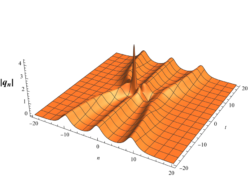
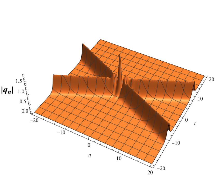
Figure 2: Left: A three-order pole solution by choosing $N=1$, $\lambda_{1}=1.5\mathrm{i}$, $m_{1}=2$ and $f(\lambda)=\lambda^{2}$; Right: Two-soliton solution by choosing $N=2$, $m_{1}=m_{2}=0$, $\lambda_{1}=1-\mathrm{i}$, $\lambda_{2}=1+\mathrm{i}$ and $f(\lambda)=1$.

5 Infinite-order soliton

Let $N=1$, $f(\lambda)=(\lambda-\lambda_{1}+\frac{1}{m_{1}+1})^{m_{1}+1}$ with $\lambda_{1}\in D_{+}$, we find $\mathbf{P}_{n}(k,\lambda;t)$ defined in Eq. (3.10) converges to the following form as $m_{1}$ tends to infinity,

$$\begin{split}\lim_{m_{1}\rightarrow\infty}\mathbf{P}_{n}(k,\lambda;t)=&\begin{pmatrix}1&0\\ -\displaystyle\lim_{m_{1}\rightarrow\infty}\theta_{n}(\lambda)\left[1+\frac{1}{(m_{1}+1)(\lambda-\lambda_{k})}\right]^{m_{1}+1}&1\end{pmatrix}\\ =&\begin{pmatrix}1&0\\ -\lambda^{-2n}\mathrm{e}^{\frac{1}{\lambda-\lambda_{1}}}&1\end{pmatrix}:=\mathbf{P}^{\infty}(\lambda;n,t).\end{split}$$ (5.1)

RH problem 3.2 becomes

Riemann–Hilbert Problem 5.1.

Find a $2\times 2$ matrix-valued function $\tilde{\mathbf{M}}^{\infty}_{n}(\lambda;t)$ that satisfies certain properties:

• Analyticity: $\tilde{\mathbf{M}}_{n}^{\infty}(\lambda;t)$ is an analytic function of $\lambda$ for $\lambda\in\mathbb{C}\backslash\{\partial\Omega_{\pm 1}\cup\partial\tilde{\Omega}_{\pm 1}\}$;

• Jump: The matrix $\tilde{\mathbf{M}}_{n}^{\infty}(\lambda;t)$ takes continuous boundary values $\tilde{\mathbf{M}}_{n\pm}^{\infty}(\lambda;t)$ from the left and right on $\partial\Omega_{\pm 1}$ oriented in a clockwise direction and $\partial\tilde{\Omega}_{\pm 1}$ oriented in a counterclockwise direction. The boundary values are related

  $$\tilde{\mathbf{M}}_{n+}^{\infty}(\lambda;t)=\tilde{\mathbf{M}}_{n-}^{\infty}(\lambda;t)\tilde{\mathbf{J}}_{n}^{\infty}(\lambda;t),\quad\lambda\in\partial\Omega_{\pm 1}\cup\partial\tilde{\Omega}_{\pm 1},$$ (5.2)

  where

  $$\tilde{\mathbf{J}}_{n}^{\infty}(\lambda;t)=\begin{cases}[\mathbf{P}^{\infty}(\lambda;n,t)]^{-1},\quad&\lambda\in\partial\Omega_{1},\\ \mathbf{P}^{\infty}(-\lambda;n,t),\quad&\lambda\in\partial\Omega_{-1},\\ [\mathbf{P}^{\infty{\dagger}}(\bar{\lambda}^{-1};n,t)]^{-1},\quad&\lambda\in\partial\tilde{\Omega}_{1},\\ \mathbf{P}^{\infty{\dagger}}(-\bar{\lambda}^{-1};n,t),\quad&\lambda\in\partial\tilde{\Omega}_{-1},\end{cases}$$ (5.3)

  with $\mathbf{P}^{\infty}(\lambda;n,t)$ is defined in Eq. (5.1);

• Normalizations: $\tilde{\mathbf{M}}_{n}^{\infty}(\lambda;t)$ has the following asymptotics:

  $$\tilde{\mathbf{M}}_{n}^{\infty}(\lambda;t)=\mathbf{I}+O(\lambda^{-1}),\qquad \lambda\rightarrow\infty,$$ (5.4a)

  $$\tilde{\mathbf{M}}_{n}^{\infty}(\lambda;t)=\begin{pmatrix}(\delta^{+}_{n})^{-1}&0\\ 0&\delta_{n}^{+}\end{pmatrix}+O(\lambda),\qquad \lambda\rightarrow 0.$$ (5.4b)

The infinite-order soliton solution $q_{n}^{\infty}(t)$ of the Ablowitz–Ladik equation (1.1) can be expressed in terms of the aforementioned RH problem 5.1:

$$q_{n}^{\infty}(t)=\lim_{\lambda\rightarrow 0}\frac{\tilde{\mathbf{M}}^{\infty}_{n+1,12}(\lambda;t)}{\lambda}.$$ (5.5)

Data availability

All data generated or analyzed during this study are including in this published article.

Declarations

Conflict of Interest

The authors declare that they have no conflict of interest.

References

- [1] M. J. Ablowitz, G. Biondini, and B. Prinari, Inverse scattering transform for the integrable discrete nonlinear Schrödinger equation with nonvanishing boundary conditions, Inverse Problems, 23 (2007), p. 1711.
- [2] M. J. Ablowitz and J. F. Ladik, Nonlinear differential-difference equations, Journal of Mathematical Physics, 16 (1975), pp. 598–603.
- [3] , Nonlinear differential-difference equations and Fourier analysis, Journal of Mathematical Physics, 17 (1976), pp. 1011–1018.
- [4] M. J. Ablowitz, B. Prinari, and A. D. Trubatch, Discrete and continuous nonlinear Schrödinger systems, vol. 302, Cambridge University Press, 2004.
- [5] T. Aktosun, F. Demontis, and C. van der Mee, Exact solutions to the focusing nonlinear Schrödinger equation, Inverse Problems, 23 (2007), pp. 2171–2195.
- [6] M. Chen and E. Fan, Riemann–Hilbert approach for discrete sine-Gordon equation with simple and double poles, Studies in Applied Mathematics, 148 (2022), pp. 1180–1207.
- [7] M. Chen, E. Fan, and J. He, -Sobolev space bijectivity of the scattering-inverse scattering transforms related to defocusing Ablowitz–Ladik systems, Physica D: Nonlinear Phenomena, 443 (2023), p. 133565.
- [8] , Riemann–Hilbert approach and the soliton solutions of the discrete mKdV equations, Chaos, Solitons & Fractals, 168 (2023), p. 113209.
- [9] Y. Ishimori, An integrable classical spin chain, Journal of the Physical Society of Japan, 51 (1982), pp. 3417–3418.
- [10] V. M. Kenkre and D. K. Campbell, Self-trapping on a dimer: Time-dependent solutions of a discrete nonlinear Schrödinger equation, Physical Review B, 34 (1986), pp. 4959–4961.
- [11] M. Li, X. Yue, and T. Xu, Multi-pole solutions and their asymptotic analysis of the focusing Ablowitz–Ladik equation, Physica Scripta, 95 (2020), p. 055222.
- [12] C. Lv and Q. Liu, Multiple higher-order pole solutions of modified complex short pulse equation, Applied Mathematics Letters, 141 (2023), p. 108518.
- [13] C. Lv, D. Qiu, and Q. P. Liu, Riemann–Hilbert approach to two-component modified short-pulse system and its nonlocal reductions, Chaos: An Interdisciplinary Journal of Nonlinear Science, 32 (2022).
- [14] E. Olmedilla, Multiple pole solutions of the non-linear Schrödinger equation, Physica D: Nonlinear Phenomena, 25 (1987), pp. 330–346.
- [15] N. Papanicolaou, Complete integrability for a discrete Heisenberg chain, Journal of Physics A: Mathematical and General, 20 (1987), p. 3637.
- [16] C. Schiebold, Asymptotics for the multiple pole solutions of the nonlinear Schrödinger equation, Nonlinearity, 30 (2017), p. 2930.
- [17] V. S. Shchesnovich and J. Yang, General soliton matrices in the Riemann–Hilbert problem for integrable nonlinear equations, Journal of Mathematical Physics, 44 (2003), pp. 4604–4639.
- [18] , Higher-Order Solitons in the N-Wave System, Studies in Applied Mathematics, 110 (2003), pp. 297–332.
- [19] S. Takeno and K. Hori, A propagating self-localized mode in a one-dimensional lattice with quartic anharmonicity, Journal of the Physical Society of Japan, 59 (1990), pp. 3037–3040.
- [20] H. Tsuru and M. Wadati, The Multiple Pole Solutions of the Sine-Gordon Equation, Journal of the Physical Society of Japan, 53 (1984), pp. 2908–2921.
- [21] M. Wadati and K. Ohkuma, Multiple-pole solutions of the modified Korteweg-de Vries equation, Journal of the Physical Society of Japan, 51 (1982), pp. 2029–2035.
- [22] B. Xia and A. Fokas, Initial–boundary value problems associated with the Ablowitz-Ladik system, Physica D: Nonlinear Phenomena, 364 (2018), pp. 27–61.
- [23] H. Yamane, Long-time asymptotics for the defocusing integrable discrete nonlinear Schrödinger equation II, SIGMA. Symmetry, Integrability and Geometry: Methods and Applications, 11 (2015), p. 020.
- [24] V. E. Zakharov and A. B. Shabat, Exact theory of two-dimensional self-focusing and one-dimensional self-modulation of waves in nonlinear media, Soviet Physics JETP, 34 (1972), pp. 62–69.
- [25] G. Zhang and Z. Yan, The derivative nonlinear Schrödinger equation with zero/nonzero boundary conditions: inverse scattering transforms and N-double-pole solutions, Journal of Nonlinear Science, 30 (2020), pp. 3089–3127.
- [26] Y. Zhang, X. Tao, and S. Xu, The bound-state soliton solutions of the complex modified KdV equation, Inverse Problems, 36 (2020), p. 065003.
- [27] Y. Zhang, X. Tao, T. Yao, and J. He, The regularity of the multiple higher-order poles solitons of the NLS equation, Studies in Applied Mathematics, 145 (2020), pp. 812–827.
- [28] X. Zhou, The Riemann–Hilbert Problem and Inverse Scattering, SIAM Journal on Mathematical Analysis, 20 (1989), pp. 966–986.