Wireless Channel Prediction via
Gaussian Mixture Models

Abstract

In this work, we utilize a Gaussian mixture model (GMM) to capture the underlying probability density function (PDF) of the channel trajectories of moving mobile terminals (MTs) within the coverage area of a base station (BS) in an offline phase. We propose to leverage the same GMM for channel prediction in the online phase. Our proposed approach does not require signal-to-noise ratio (SNR)-specific training and allows for parallelization. Numerical simulations for both synthetic and measured channel data demonstrate the effectiveness of our proposed GMM-based channel predictor compared to state-of-the-art channel prediction methods.

I Introduction

To achieve high data rates in wireless communications systems, the knowledge of channel state information (CSI) at the BS is a crucial prerequisite. In scenarios where the MTs are moving along trajectories, the CSI knowledge gets outdated. Therefore, accurate CSI prediction, which aims to forecast upcoming CSI given past observations corrupted by noise, is highly important.

Classical techniques that utilize linear prediction filters were proposed in, e.g., [1, 2, 3]. More recently, non-linear techniques, especially neural network (NN)-based solutions, were proposed for channel prediction in, e.g., [4, 5, 6]. Both classical and NN-based techniques require the velocity knowledge of the moving MT and/or are specifically trained for a particular SNR level. In the case of the NN-based approaches, in addition to the burden of training many specialized NNs, a separate network needs to be stored for each velocity and/or SNR configuration.

Recently, GMMs (cf. [7, Sec. 9.2]) were utilized to capture the underlying PDF of any channel that stems from a particular communications environment and were used for, e.g., channel estimation in [8] and precoding in [9]. Motivated by the universal approximation property of GMMs (see [10]), we propose to utilize GMMs for channel prediction in this work to address the aforementioned drawbacks of classical and NN-based techniques.

Contributions: We utilize the discrete latent space of GMMs to derive an approximate minimum mean squared error (MSE)-optimal channel predictor for given noisy observations that is composed of an observation-dependent convex combination of linear minimum mean squared error (LMMSE) prediction filters. A key feature of our proposed GMM predictor is that after fitting a single GMM at the BS to a training set of trajectories with a predefined length in the offline phase, the same GMM can be used online for channel prediction with customized observation and prediction intervals. Moreover, the GMM supports channel prediction for any desired SNR level and neither requires retraining nor the knowledge of the velocities of the MTs. Numerical results for both synthetic and measured channel data demonstrate the superior performance of our proposed method compared to state-of-the-art channel prediction approaches.

II System Model and Channel Data

The channel coefficients along a trajectory of a moving MT are denoted by $h[m]$, with $m=0,\dots,M_{\mathrm{o}}+N_{\mathrm{p}}-1$, where $M_{\mathrm{o}}$ is the observation length, and $N_{\mathrm{p}}$ is the prediction length. During the symbol duration $T_{\mathrm{S}}$, the channel coefficients $h[m]$ are assumed to remain constant. The goal of this work is to predict any desired channel coefficient out of the prediction interval $\mathcal{I}_{N_{\mathrm{p}}}=\{M_{\mathrm{o}},M_{\mathrm{o}}+1,\dots,M_{\mathrm{o}}+N_{\mathrm{p}}-1\}$, given noisy observations of the channel coefficients of the observation interval $\mathcal{I}_{M_{\mathrm{o}}}=\{0,1,\dots,M_{\mathrm{o}}-1\}$. Thus, the BS receives

$$\bm{y}=\bm{h}_{M_{\mathrm{o}}}+\bm{n}\in\mathbb{C}^{M_{\mathrm{o}}}$$ (1)

where $\bm{h}_{M_{\mathrm{o}}}=[h[M_{\mathrm{o}}-1],h[M_{\mathrm{o}}-2],\dots,h[1],h[0]]^{\operatorname{T}}$ comprises the channel coefficients of the observation interval $\mathcal{I}_{M_{\mathrm{o}}}$, and $\bm{n}\sim\mathcal{N}_{\mathbb{C}}(\mathbf{0},{\bm{\Sigma}}=\sigma^{2}\mathbf{I}_{M_{\mathrm{o}}})$ denotes additive white Gaussian noise (AWGN).

With $\bm{h}$, we denote the vector of channel coefficients of the observation interval $\mathcal{I}_{M_{\mathrm{o}}}$ extended by all of the coefficients of the prediction interval $\mathcal{I}_{N_{\mathrm{p}}}$, i.e., $\bm{h}=[{h[M_{\mathrm{o}}+N_{\mathrm{p}}-1]},{h[M_{\mathrm{o}}+N_{\mathrm{p}}-2]},\dots,{h[M_{\mathrm{o}}]},\bm{h}_{M_{\mathrm{o}}}^{\operatorname{T}}]^{\operatorname{T}}\in\mathbb{C}^{M_{\mathrm{o}}+N_{\mathrm{p}}}$. We have that

$$\bm{h}_{M_{\mathrm{o}}}=\bm{S}^{\operatorname{T}}\bm{h}$$ (2)

with the selection matrix $\bm{S}=\begin{bmatrix}\mathbf{0},\mathbf{I}_{M_{\mathrm{o}}}\end{bmatrix}^{\operatorname{T}}\in\{0,1\}^{M_{\mathrm{o}}+N_{\mathrm{p}}\times M_{\mathrm{o}}}$.

With

$$\mathcal{H}=\{\bm{h}_{j}\}_{j=1}^{J},$$ (3)

we denote the training data set consisting of $J$ trajectories. We consider two different data sources in this work, briefly outlined next.

II-A Synthetic Channel Data

We utilize the QuaDRiGa channel simulator [11, 12] to generate channel trajectories in an urban macrocell (UMa) scenario. We consider a single-carrier with a carrier frequency $f_{\mathrm{c}}=$3.5\text{\,}\mathrm{GHz}$$ and the symbol duration is $T_{\mathrm{S}}=$0.5\text{\,}\mathrm{m}\mathrm{s}$$. Placed at a height of $20\text{\,}\mathrm{m}$, the BS covers a $120$\text{\,}\mathrm{\SIUnitSymbolDegree}$$ sector. The MTs are outdoors and move along straight trajectories with a constant velocity $v$, uniformly drawn from 3 to 100 km/h, at a height of $1.5\text{\,}\mathrm{m}$. The BS and each MT are equipped with single antennas. The distances between the MTs and the BS are randomly drawn between $35\text{\,}\mathrm{m}$ and $500\text{\,}\mathrm{m}$. Following the description in the QuaDRiGa manual [12], the path gain of the generated channel trajectories is normalized.

II-B Measured Channel Data

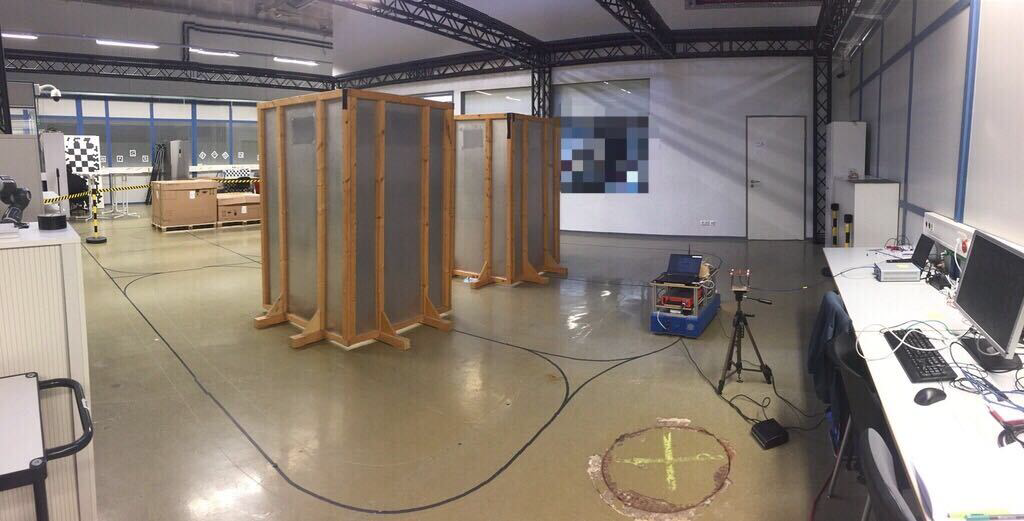
Figure 1: Industrial hall—Measurement site [13]. In this scenario, the blue AGV with attached measurement hardware moves around both obstacles.

Since synthetic channel data generally does not fully characterize the features of real-world environments, we utilize channel data measured in an industrial hall to assess the performance of the proposed channel predictor under real-world conditions. A detailed description of the measurement campaign can be found in [13]. The dataset and supplementary material are available in [14]. The measurement area is modified to consider changing environments by placing obstacles at certain positions and capturing ten different measurement scenarios. In Fig. 1, we depict exemplarily a measurement scenario where the automated guided vehicle (AGV) moves around obstacles. To facilitate generalization to different sub-carriers, which ranged from $3.7\text{\,}\mathrm{GHz}$ to $3.8\text{\,}\mathrm{GHz}$, and measurement scenarios, the training set and the test set consist of trajectories stemming from all available sub-carriers and measurement scenarios. An AGV moving along predefined trajectories with a fixed velocity of $v=$1\text{\,}\mathrm{m}\mathrm{/}\mathrm{s}$$ mimics the moving MT, whereby the symbol duration is $T_{\mathrm{S}}=$1\text{\,}\mathrm{m}\mathrm{s}$$. The issue outlined in [15], concerning a fractional sampling time offset due to lack of synchronization between the transmitter and receiver, leads to an extra, subcarrier-specific phase drift over time in the channel frequency response. With continuously measured data available, this phase drift can be tracked and corrected using linear regression in a post-processing step.

III Channel Prediction via GMMs

The stochastic nature of all channel trajectories in the whole coverage area of the BS is described by a PDF $f_{\bm{h}}$. Every channel trajectory $\bm{h}$ of any moving MT within the environment is a realization of a random variable with PDF $f_{\bm{h}}$. Motivated by the universal approximation property of GMMs [10], we make use of a GMM to approximate the PDF $f_{\bm{h}}$ in an offline phase. Thereby, we learn the joint channel distribution of the observation and the prediction interval via the training dataset $\mathcal{H}$ defined in (3) and, thus, are able to capture the dependencies between the observations and the CSI values that should be predicted later in the inference/online phase.

III-A Capturing the Environment – Offline

A GMM with $K$ components is a PDF of the following form:

$$f^{(K)}_{\bm{h}}(\bm{h})=\sum\nolimits_{k=1}^{K}\pi_{k}\mathcal{N}_{\mathbb{C}}(\bm{h};{\bm{\mu}}_{k},\bm{C}_{k}).$$ (4)

The GMM components are described by the mixing coefficients $\pi_{k}$, means ${\bm{\mu}}_{k}$, and covariances $\bm{C}_{k}$, where maximum likelihood estimates of these parameters can be obtained with an expectation-maximization (EM) algorithm given the training dataset $\mathcal{H}$ in (3), cf. [7, Subsec. 9.2.2].

Based on the GMM, the posterior probability (also called responsibility) that a particular channel trajectory stems from component $k$ is given by [7, Sec. 9.2]

$$p(k\mid\bm{h})=\frac{\pi_{k}\mathcal{N}_{\mathbb{C}}(\bm{h};{\bm{\mu}}_{k},\bm{C}_{k})}{\sum_{i=1}^{K}\pi_{i}\mathcal{N}_{\mathbb{C}}(\bm{h};{\bm{\mu}}_{i},\bm{C}_{i})}.$$ (5)

The joint Gaussianity of each GMM component [see (4)] together with the AWGN allows to compute the GMM of the observations via [see (1) and (2)]

$$f_{\bm{y}}^{(K)}(\bm{y})=\sum\nolimits_{k=1}^{K}\pi_{k}\mathcal{N}_{\mathbb{C}}(\bm{y};\bm{S}^{\operatorname{T}}{\bm{\mu}}_{k},\bm{S}^{\operatorname{T}}\bm{C}_{k}\bm{S}+{\bm{\Sigma}}).$$ (6)

Accordingly, the responsibilities given noisy observations are computed as

$$p(k\mid\bm{y})=\frac{\pi_{k}\mathcal{N}_{\mathbb{C}}(\bm{y};\bm{S}^{\operatorname{T}}{\bm{\mu}}_{k},\bm{S}^{\operatorname{T}}\bm{C}_{k}\bm{S}+{\bm{\Sigma}})}{\sum_{i=1}^{K}\pi_{i}\mathcal{N}_{\mathbb{C}}(\bm{y};\bm{S}^{\operatorname{T}}{\bm{\mu}}_{i},\bm{S}^{\operatorname{T}}\bm{C}_{i}\bm{S}+{\bm{\Sigma}})}.$$ (7)

III-B Channel Prediction – Online

In the online phase, we aim to predict a single channel coefficient $h_{\ell}=h[M_{\mathrm{o}}-1+\ell]$, which lies $\ell$ steps in the future of the last observed channel coefficient $h[M_{\mathrm{o}}-1]$, with a given noisy observation $\bm{y}$ from (1). In this work, we try to approximate the conditional mean estimator (CME), given by

$$\operatorname{E}\left[h_{\ell}\mid\bm{y}\right]$$ (8)

which is the MSE-optimal predictor [3, Sec. 11.4]. Since we have learned a GMM $f^{(K)}_{\bm{h}}$ for the joint distribution $f_{\bm{h}}$, we can compute the CME over this approximate GMM distribution, denoted by

$$\hat{h}_{\text{GMM}}=\operatorname{E}^{(K)}\left[h_{\ell}\mid\bm{y}\right].$$ (9)

Conveniently, this GMM-based CME can be computed in closed-form by utilizing the law of total expectation such that

$$\hat{h}_{\text{GMM}} =\operatorname{E}\left[\operatorname{E}^{(K)}[h_{\ell}\mid\bm{y},k]\mid\bm{y}\right]$$ (10)

$$=\sum_{k=1}^{K}p(k\mid\bm{y})\operatorname{E}^{(K)}\left[h_{\ell}\mid\bm{y},k\right]$$ (11)

with the responsibilities of the observations from (7). Due to the Gaussianity of each GMM component, the channel and observation become jointly Gaussian when conditioned on a GMM component. Thus, the conditional expectation in (11) is computed by LMMSE predictions of the form

$$\operatorname{E}^{(K)}[ h_{\ell}\mid\bm{y},k]=\bm{c}_{\bm{y},h_{\ell}|k}^{\operatorname{H}}\bm{C}_{\bm{y}|k}^{-1}(\bm{y}\!-\!{{\bm{\mu}}}_{\bm{y}|k})\!+\mu_{h_{\ell}|k}$$ (12)

$$=\mathbf{e}_{\ell}^{\operatorname{T}}\bm{C}_{k}\bm{S}(\bm{S}^{\operatorname{T}}\bm{C}_{k}\bm{S}\!+\!{\bm{\Sigma}})^{-1}(\bm{y}\!-\!\bm{S}^{\operatorname{T}}{{\bm{\mu}}}_{k})\!+\mathbf{e}_{\ell}^{\operatorname{T}}{{\bm{\mu}}}_{k}$$

where $\mathbf{e}_{\ell}\in\{0,1\}^{M_{\mathrm{o}}+N_{\mathrm{p}}}$, which contains a one at the $\ell$-th entry and is zero elsewhere, cuts out the channel coefficient of interest since $h_{\ell}=\mathbf{e}_{\ell}^{\operatorname{T}}\bm{h}$. For a detailed analysis of the asymptotic behavior of the approximate CME via the GMM from (9) and the true CME from (8), we refer the interested reader to [8]. A considerable advantage of the GMM-based prediction approach is that it does not require retraining for different SNR levels since the GMM of the observations in (6) can be adapted depending on the noise statistics.

III-C Complexity Analysis

The prediction filters $\mathbf{e}_{\ell}^{\operatorname{T}}\bm{C}_{k}\bm{S}(\bm{S}^{\operatorname{T}}\bm{C}_{k}\bm{S}\!+\!{\bm{\Sigma}})^{-1}$ in (12) can be precomputed offline for a given SNR level since the GMM parameters do not change after the fitting process. Thus, evaluating the conditional expectation in (12) has a complexity of only $\mathcal{O}(M_{\mathrm{o}}+\ell)$. To obtain a predicted channel coefficient, the computation of the responsibilities of the observations is further needed, which requires evaluating Gaussian densities, cf. (7). Due to the fixed GMM parameters, the online evaluation of the responsibilities is dominated by matrix-vector multiplications with a complexity of $\mathcal{O}(M_{\mathrm{o}}^{2})$. Overall, evaluating (11) has a total complexity of $\mathcal{O}(KM_{\mathrm{o}}^{2})$. Note that parallelization with respect to the number of components $K$ is possible.

III-D Structural Constraints

Due to model-based insights, the number of GMM parameters can be reduced by constraining the GMM covariance matrices. Exploiting model-based insights has already been advantageous for applications such as channel estimation in [16] and precoding in [17]. In general, structural constraints reduce the number of parameters that need to be learned, lower the offline training complexity, and reduce the number of required training samples. In this work, we will constrain the GMM covariances to be Toeplitz, which can be expressed as

$$\bm{C}_{k}=\bm{Q}^{\operatorname{H}}\operatorname{diag}(\bm{c}_{k})\bm{Q}$$ (13)

where $\bm{Q}$ contains the first $M_{\mathrm{o}}+N_{\mathrm{p}}$ columns of a $2(M_{\mathrm{o}}+N_{\mathrm{p}})\times 2(M_{\mathrm{o}}+N_{\mathrm{p}})$ discrete Fourier transform (DFT) matrix, and $\bm{c}_{k}\in\mathbb{R}_{+}^{2(M_{\mathrm{o}}+N_{\mathrm{p}})}$ [6, 18]. Thus, the structural constraints allow storing only the vectors $\bm{c}_{k}$, $k=1,\dots,K$, of a GMM, drastically reducing the memory requirement and the number of parameters to be learned without affecting the online prediction complexity compared to a GMM with full covariance matrices.

IV Baseline Channel Predictors

We consider the following baseline channel predictors. A predicted channel coefficient can be obtained, for example, with the LMMSE predictor [3]

$$\hat{h}_{\text{LMMSE}}=\mathbf{e}_{\ell}^{\operatorname{T}}\bm{C}_{s}\bm{S}(\bm{S}^{\operatorname{T}}\bm{C}_{s}\bm{S}\!+\!{\bm{\Sigma}})^{-1}\bm{y}$$ (14)

which utilizes the sample covariance matrix $\bm{C}_{s}=\frac{1}{J}\sum_{j=1}^{J}\bm{h}_{j}\bm{h}_{j}^{\operatorname{H}}$ using the same channel trajectories which are used for fitting the GMM, i.e., the training dataset $\mathcal{H}$ [see (3)] is used.

Alternatively, the LMMSE predictor based on assuming that the spectrum of the signal follows Jakes’ spectrum, which describes the temporal evolution of the channel in the one-ring channel model, cf. [1, 19, 3], is computed as

$$\hat{h}_{\text{LMMSE Jakes}}=\mathbf{e}_{\ell}^{\operatorname{T}}\bm{C}_{\text{Jakes}}\bm{S}(\bm{S}^{\operatorname{T}}\bm{C}_{\text{Jakes}}\bm{S}\!+\!{\bm{\Sigma}})^{-1}\bm{y}.$$ (15)

The covariance matrix $\bm{C}_{\text{Jakes}}$ is a Toeplitz-structured real-valued matrix, where its top row is given by the zeroth order Bessel function $J_{0}(2\pi mT_{\mathrm{S}}f_{\mathrm{c}}{v}/{\mathrm{c}})$, cf. [1, 19, 20]. Note that the exact knowledge of the velocity $v$ is a prerequisite for the LMMSE Jakes predictor. We further consider the LMMSE Jakes predictor, where we assume either a $10\%$ or $20\%$ velocity estimation error since, in the online phase, a MT’s velocity must be inferred from the noisy observations $\bm{y}$.

Lastly, we compare to the NN-based channel predictor from [6], which infers a prediction filter from transformed noisy observations $\hat{\bm{c}}={\frac{1}{\sigma^{2}}}|\bm{Q}_{\text{NN}}\bm{y}|^{2}$ [$\bm{Q}_{\text{NN}}$ is similarly defined as in (13)] at the input of the NN and applies it to the observations to compute a predicted coefficient:

$$\hat{h}_{\text{NN}}=\hat{\bm{w}}^{\operatorname{T}}(\hat{\bm{c}})\bm{y}.$$ (16)

A drawback of the NN-based prediction approach is that it requires training for each SNR level. Details about the network architecture and the hyper-parameters can be found in [6].

Figure 2: Channel prediction error over the SNR for a system with $M_{\mathrm{o}}=19$, $\ell=1$, and $K=128$ (synthetic channel data).

V Experiments and Results

In our simulations, the SNR is defined as $\frac{1}{\sigma^{2}}$, since we normalized the data such that $\operatorname{E}[\|\bm{h}\|^{2}]=M_{\mathrm{o}}+N_{\mathrm{p}}$. To assess the prediction performance, we utilize the MSE $\frac{1}{T}\sum_{{t}=1}^{T}|h_{t}[m]-\hat{h}_{t}[m]|^{2}$ as performance measure and use $T=10{,}000$ test samples. We utilize $J=150{,}000$ training samples for fitting the GMM and for training the NNs.

Figure 3: Channel prediction error over the number of components $K$, for a system with $M_{\mathrm{o}}=19$, $\ell=1$, and SNR $=$20\text{\,}\mathrm{dB}$$ (synthetic channel data).

V-A Experiments with Synthetic Channel Data

Firstly, we present simulation results using the synthetic channel data described in Subsection II-A. In Fig. 2, we depict the prediction error over the SNR, for an observation length of $M_{\mathrm{o}}=19$, and we predict one step into the future, i.e., $\ell=1$. We set the number of GMM components to $K=128$. We can observe that the GMM performs best, followed by the GMM with the Toeplitz structure enforced on the covariance matrices (denoted by “Toeplitz GMM”). The “LMMSE Jakes Perfect” predictor performs almost equally well but, in contrast to the GMM-based predictor, requires the exact knowledge of the MT’s velocity. We can observe a severe performance degradation by artificially introducing a velocity estimation error, cf. “LMMSE Jakes ($\pm 10\%$)” and “LMMSE Jakes ($\pm 20\%$)”. The NN approach (denoted by “NN”) performs worse than the GMM and achieves a similar performance as “LMMSE Jakes ($\pm 10\%$)”. The NN approach also does not require the knowledge of the velocity as the GMM-based predictor but requires separate training for each SNR level. In principle, a NN for the whole SNR range can be learned, but a NN trained for a large range of SNR levels generally exhibits a worse performance, cf. e.g., [21].

In Fig. 3, we simulate the same setup but fix the SNR to $20\text{\,}\mathrm{dB}$ and vary the number of components $K$ of the GMM-based predictors. Accordingly, all baselines remain constant since they do not depend on $K$. With an increasing number of components, the prediction performance steadily increases and exhibits a saturation for $K>16$. Both of the GMM-based predictors outperform most baselines with only a few components. We can observe that the Toeplitz constraint comes at the cost of slightly degraded performance and requires approximately $32$ components to outperform “LMMSE Jakes Perfect” as opposed to the GMM with full covariances, which only requires $16$ components.

V-B Experiments with Measured Channel Data

Figure 4: Channel prediction error over the SNR for a system with $M_{\mathrm{o}}=19$, $\ell=1$, and $K=128$ (measured channel data).

In the remainder, we focus our numerical evaluation on the measured channel data described in Subsection II-B. In Fig. 4, we depict the prediction error over the SNR for an observation length of $M_{\mathrm{o}}=19$, and we predict one step into the future, i.e., $\ell=1$. We set the number of GMM components to $K=128$. In alignment with the results for the synthetic data, also in the case of measured data, the GMM performs best, followed by the GMM with the Toeplitz structure enforced on the covariance matrices (“Toeplitz GMM”). In contrast to the synthetic channel data simulations, we can observe a huge performance degradation of the “LMMSE Jakes Perfect” predictor, due to the one-ring model assumption of Jakes, which is not fulfilled in the indoor factory hall measurement environment, especially, in the presence of a line of sight (LOS) condition. The artificially introduced velocity estimation errors, cf. “LMMSE Jakes ($\pm 10\%$)” and “LMMSE Jakes ($\pm 20\%$)” lead to further performance degradations in this case. Furthermore, the NN approach with SNR level-specific training (“NN”) performs slightly worse than the GMM.

In Fig. 5, we depict the prediction error over the SNR, for an observation length of $M_{\mathrm{o}}=16$, and we predict four steps into the future, i.e., $\ell=4$, and keep $K=128$. We can observe that compared to the simulation setting in Fig. 4, all of the approaches perform worse since the prediction task is harder with fewer observations ($M_{\mathrm{o}}=16$ instead of $19$) and with a larger prediction step ($\ell=4$ instead of $1$). The ordering of the performances of the prediction approaches remains the same, but the performance gap of the GMM-based predictor compared to the “LMMSE” and “LMMSE Jakes Perfect” increased.

Lastly, in Fig. 6, we evaluate a setup with $M_{\mathrm{o}}=16$, $K=128$, fix the SNR at $20\text{\,}\mathrm{dB}$, and vary the prediction step $\ell$. As explained above, the GMM-based prediction approach is trained once for the overall trajectory of length $20$ and is customized to the different prediction steps $\ell\in\{1,2,3,4\}$. It yields the best performance, followed by the GMM with the Toeplitz structure enforced on the covariance matrices (“Toeplitz GMM”). With “NN, $\ell_{\text{train}}\in\{1,2,3,4\}$”, we denote the NN approaches trained for fixed prediction steps $\ell_{\text{train}}$, where the obtained predicted coefficient in the online phase is taken as representative for the prediction step $\ell$ of interest. We can see that each NN trained for a specific prediction step $\ell_{\text{train}}$ performs best if the prediction step of interest $\ell$ is equal to $\ell_{\text{train}}$, thus, highlighting the need for a NN specifically trained for a particular prediction step in addition to the SNR level.

Figure 5: Channel prediction error over the SNR for a system with $M_{\mathrm{o}}=16$, $\ell=4$, and $K=128$ (measured channel data).

VI Conclusion and Future Work

We proposed a wireless channel predictor based on GMMs and assessed its performance with synthetic and measured channel data. Once the GMM is trained for a predefined trajectory length in the offline phase, it can be customized for varying observations and prediction lengths in the online phase without requiring retraining for different SNR levels. The GMM-based channel predictor even allows for multiple predictions simultaneously by adapting the prediction filters in (12) accordingly. Future work aims to explore an extension to systems with multiple antennas and systems involving coarse quantization, cf., e.g., [22, 23]. Moreover, other generative modeling-based techniques, such as variational autoencoders, could be utilized as generative priors for channel prediction similar to the channel estimation case as in [24].

Figure 6: Channel prediction error over the prediction step $\ell$, for a system with $M_{\mathrm{o}}=16$, $K=128$, and SNR $=$20\text{\,}\mathrm{dB}$$ (measured channel data).

References

- [1] T. Zemen, C. F. Mecklenbrauker, F. Kaltenberger, and B. H. Fleury, “Minimum-energy band-limited predictor with dynamic subspace selection for time-variant flat-fading channels,” IEEE Trans. Signal Process., vol. 55, pp. 4534–4548, 2007.
- [2] K. Baddour and N. Beaulieu, “Autoregressive modeling for fading channel simulation,” IEEE Trans. Wireless Commun., vol. 4, no. 4, pp. 1650–1662, 2005.
- [3] S. Kay, Fundamentals of Statistical Signal Processing: Estimation Theory. Prentice-Hall, 1993.
- [4] H. Jiang, M. Cui, D. W. K. Ng, and L. Dai, “Accurate channel prediction based on transformer: Making mobility negligible,” IEEE J. Sel. Areas Commun., vol. 40, no. 9, pp. 2717–2732, 2022.
- [5] J. Yuan, H. Q. Ngo, and M. Matthaiou, “Machine learning-based channel estimation in massive MIMO with channel aging,” in IEEE 20th Int. Workshop Signal Process. Advances in Wireless Commun. (SPAWC), 2019, pp. 1–5.
- [6] N. Turan and W. Utschick, “Learning the MMSE channel predictor,” in IEEE Int. Conf. Commun. Workshops (ICC Workshops), 2020, pp. 1–6.
- [7] C. M. Bishop, Pattern Recognition and Machine Learning (Information Science and Statistics). Berlin, Heidelberg: Springer-Verlag, 2006.
- [8] M. Koller, B. Fesl, N. Turan, and W. Utschick, “An asymptotically MSE-optimal estimator based on Gaussian mixture models,” IEEE Trans. Signal Process., vol. 70, pp. 4109–4123, 2022.
- [9] N. Turan, B. Fesl, M. Koller, M. Joham, and W. Utschick, “A versatile low-complexity feedback scheme for FDD systems via generative modeling,” IEEE Trans. Wireless Commun., early access, Nov. 14, 2023, doi: 10.1109/TWC.2023.3330902.
- [10] T. T. Nguyen, H. D. Nguyen, F. Chamroukhi, and G. J. McLachlan, “Approximation by finite mixtures of continuous density functions that vanish at infinity,” Cogent Math. Statist., vol. 7, no. 1, p. 1750861, 2020.
- [11] S. Jaeckel, L. Raschkowski, K. Börner, and L. Thiele, “Quadriga: A 3-d multi-cell channel model with time evolution for enabling virtual field trials,” IEEE Trans. Antennas Propag., vol. 62, no. 6, pp. 3242–3256, 2014.
- [12] S. Jaeckel, L. Raschkowski, K. Börner, L. Thiele, F. Burkhardt, and E. Eberlein, “Quadriga: Quasi deterministic radio channel generator, user manual and documentation,” Fraunhofer Heinrich Hertz Inst., Berlin, Germany, Tech. Rep. v2.2.0, 2019.
- [13] F. Burmeister, N. Schwarzenberg, T. Hößler, and G. Fettweis, “Measuring time-varying industrial radio channels for D2D communications on AGVs,” in IEEE Wireless Commun. Netw. Conf. (WCNC), 2021, pp. 1–7.
- [14] F. Burmeister and N. Schwarzenberg, “Data set for time-varying industrial radio channels in varying environment,” 2023. [Online]. Available: https://dx.doi.org/10.21227/htgs-jp87
- [15] F. Burmeister, R. Jacob, A. Traßl, N. Schwarzenberg, and G. Fettweis, “Dealing with fractional sampling time offsets for unsynchronized mobile channel measurements,” IEEE Wireless Communications Letters, vol. 10, no. 12, pp. 2781–2785, 2021.
- [16] B. Fesl, M. Joham, S. Hu, M. Koller, N. Turan, and W. Utschick, “Channel estimation based on Gaussian mixture models with structured covariances,” in 56th Asilomar Conf. Signals, Syst., Comput., 2022, pp. 533–537.
- [17] N. Turan, B. Fesl, and W. Utschick, “Enhanced low-complexity FDD system feedback with variable bit lengths via generative modeling,” in 57th Asilomar Conf. Signals, Syst., Comput., 2023, to be published, arXiv preprint: 2305.03427.
- [18] G. Strang, “A proposal for Toeplitz matrix calculations,” Stud. in Appl. Math., vol. 74, no. 2, pp. 171–176, 1986.
- [19] A. Goldsmith, Wireless Communications. Cambridge Univ. Press, 2005.
- [20] W. Jakes, Microwave Mobile Communications. Wiley, 1974.
- [21] M. B. Mashhadi and D. Gündüz, “Pruning the pilots: Deep learning-based pilot design and channel estimation for MIMO-OFDM systems,” IEEE Trans. Wireless Commun., vol. 20, no. 10, pp. 6315–6328, 2021.
- [22] B. Fesl, N. Turan, B. Böck, and W. Utschick, “Channel estimation for quantized systems based on conditionally Gaussian latent models,” 2023, arXiv preprint: 2309.04014.
- [23] N. Turan, M. Koller, and W. Utschick, “One-bit quantized channel prediction with neural networks,” in 2021 IEEE 32nd Annu. Int. Symp. Pers., Indoor Mobile Radio Commun. (PIMRC), 2021, pp. 604–609.
- [24] B. Böck, M. Baur, V. Rizzello, and W. Utschick, “Variational inference aided estimation of time varying channels,” in IEEE Int. Conf. Acoust., Speech Signal Process, (ICASSP), 2023, pp. 1–5.