BBox-Adapter: Lightweight Adapting for Black-Box Large Language Models

Abstract

Adapting state-of-the-art Large Language Models (LLMs) like GPT-4 and Gemini for specific tasks is challenging. Due to the opacity in their parameters, embeddings, and even output probabilities, existing fine-tuning adaptation methods are inapplicable. Consequently, adapting these black-box LLMs is only possible through their API services, raising concerns about transparency, privacy, and cost. To address these challenges, we introduce BBox-Adapter, a novel lightweight adapter for black-box LLMs. BBox-Adapter distinguishes target and source domain data by treating target data as positive and source data as negative. It employs a ranking-based Noise Contrastive Estimation (NCE) loss to promote the likelihood of target domain data while penalizing that of the source domain. Furthermore, it features an online adaptation mechanism, which incorporates real-time positive data sampling from ground-truth, human, or AI feedback, coupled with negative data from previous adaptations. Extensive experiments demonstrate BBox-Adapter’s effectiveness and cost efficiency. It improves model performance by up to $6.77\%$ across diverse tasks and domains, while reducing training and inference costs by $31.30$x and $1.84$x, respectively.

Table 1: Comparison of existing LLM adaptation methods based on five aspects: (1) Model parameters accessibility, (2) Access to high-dimensional representations of input sequences or output generations, (3) Token probability availability, (4) Retrieval corpus necessity, and (5) Utilization of a smaller adapter model.

Methods	w/o Model Parameters	w/o High-Dimensional Representation	w/o Token Probabilities	w/o Retrieval Corpus	w/ Smaller Adapter
White-Box LLM Fine-Tuning
Fine-Tuning (Devlin et al., 2019)	✗	✗	✗	✓	✗
Instruction-Tuning (Wei et al., 2021)	✗	✗	✗	✓	✗
Continual Pre-Training (Gururangan et al., 2020)	✗	✗	✗	✓	✗
Adapter (Houlsby et al., 2019)	✗	✗	✗	✓	✓
Prefix-Tuning (Liu et al., 2022)	✗	✗	✗	✓	✓
LoRA (Hu et al., 2021)	✗	✗	✗	✓	✓
Grey-Box LLM Adaptation
LMaaS (Sun et al., 2022)	✓	✗	✗	✓	✓
kNN-Adapter (Huang et al., 2023)	✓	✓	✗	✗	✓
CombLM (Ormazabal et al., 2023)	✓	✓	✗	✓	✓
Proxy-Tuning (Liu et al., 2024)	✓	✓	✗	✓	✓
Black-Box LLM Adaptation
BBox-Adapter (Ours)	✓	✓	✓	✓	✓

1 Introduction

Figure 1: Illustration of white-box, grey-box, and black-box LLM adaptation. White-box has complete access to both model parameters and output probabilities, grey-box has access only to output probabilities, and black-box lacks access to both. indicates the models with trainable parameters, whereas indicates the inaccessible fixed parameters.

Large Language Models (LLMs) have demonstrated exceptional abilities in comprehending and generating text across a wide range of tasks (Radford et al., 2018, 2019; Brown et al., 2020; OpenAI, 2023; Chowdhery et al., 2022). Despite their growing capabilities, general-purpose, pre-trained LLMs still require further customization to achieve optimal performance on specific use cases. However, adapting black-box LLMs like GPT-3.5 (OpenAI, 2022) and Gemini (Team et al., 2023) presents significant challenges due to the lack of direct access to internal model parameters.

Adapting black-box LLMs can be achieved by preparing and uploading training data through fine-tuning APIs, such as the OpenAI GPT-3.5-turbo fine-tuning API (Peng et al., 2023). However, employing fine-tuning APIs for LLM adaptation has several critical issues: (1) Transparency: Aside from a restricted set of adjustable hyperparameters (e.g., the number of tuning epochs), the fine-tuning process remains largely opaque. Crucial aspects, such as the extent of trainable layers and specific model weights, are often undisclosed, hindering optimal customization. (2) Privacy: Uploading training data via APIs introduces potential risks of privacy breaches, limiting the use of LLMs in sensitive domains. For instance, electronic health records containing confidential healthcare information require stringent privacy measures. (3) Cost: The cost associated with fine-tuning APIs is considerably higher compared to inference, making the adaptation expensive. The fine-tuning cost will significantly increase with hyperparameter tuning.

The adaptation of black-box LLMs without the use of APIs remains an unresolved challenge. Recent studies have explored adapting LLMs without accessing model weights, by integrating outputs with tunable white-box models (Sun et al., 2022; Ormazabal et al., 2023; Liu et al., 2024) or external data sources (Huang et al., 2023). However, such approaches (depicted as grey-box adaptation in Figure 1) still require access to the token probabilities of the output sequences, only available in models preceding GPT-3 (Brown et al., 2020) or white-box LLMs like LLaMA-2 (Touvron et al., 2023). Output probabilities, unfortunately, are inaccessible in recent black-box LLMs like GPT-3.5 (OpenAI, 2022) and PaLM-2 (Anil et al., 2023), making these techniques inapplicable for state-of-the-art black-box LLMs.

We propose BBox-Adapter, a lightweight adapter that adapts black-box LLMs for specific tasks by fine-tuning a smaller language model (LM) with just 0.1B-0.3B parameters. We formulate the black-box LLM adaptation process as a sampling problem from an energy-based model (EBM). To effectively distinguish between source and target domain data, we design a ranking-based noise contrastive estimation (NCE) loss for adapter updates. We combine outputs from the black-box LLM and the adapter for adaptive inference. BBox-Adapter employs an online adaptation framework, iteratively sampling from previous inferences and updating the adapter. Notably, the adapter facilitates self-improvement through AI feedback during training, reducing the reliance on ground-truth training data as positive samples in the online adaptation process.

Extensive experiments across three diverse datasets demonstrate the effectiveness of BBox-Adapter in adapting black-box LLMs to downstream tasks, achieving performance gains of up to $6.77\%$, while significantly reducing training and inference costs of fine-tuning methods. Moreover, BBox-Adapter accomplishes black-box LLM adaptation without requiring access to model parameters or output probabilities, enabling transparent, privacy-conscious, and cost-effective customization of cutting-edge LLMs. We summarize the main contributions as follows:

$\bullet$ We first categorize the adaptation methods systematically based on the accessible information for the algorithms.

$\bullet$ We introduce BBox-Adapter, a novel energy-based adapter that fine-tunes a smaller LM to facilitate black-box LLM adaptation without fine-tuning APIs. To the best of our knowledge, BBox-Adapter is the first black-box adapter to enable state-of-the-art LLM (e.g., GPT-3.5) adaptation without model weights or output probabilities.

$\bullet$ BBox-Adapter is lightweight, using a small model with just 0.1B-0.3B parameters as the adapter. It surpasses supervised fine-tuning (SFT) by 31.30 times during training and 1.84 times during inference in terms of cost.

$\bullet$ BBox-Adapter is also applicable without ground-truth data for the task. Its online adaptation framework can use negative samples from previous model inferences and positive samples from various sources, including AI feedback. This allows BBox-Adapter to remain effective even when ground-truth data is limited or unavailable.

$\bullet$ BBox-Adapter offers a generalizable and flexible solution for LLM adaptation. It can be applied to a wide range of tasks, domains, and models of varying sizes. Once the adapter is tuned for a specific task or domain, it can be directly applied to other black-box LLMs in a plug-and-play manner, eliminating the need for further retraining.

2 Categorization of LLM Adaptation

Based on the accessibility to internal model parameters and output probabilities, we categorize LLM adaptation methods into three main groups (Table 1): white-box fine-tuning (full access), grey-box adaptation (access to output probabilities only), and black-box adaptation (no access).

White-Box LLM Fine-Tuning. To fully leverage the capabilities of LLMs in language comprehension and enhance their performance, many users still need to customize them for specific tasks and domains (Chung et al., 2022). A straightforward approach to achieve this involves fine-tuning (Wei et al., 2021; Wang et al., 2022b) or continuous pre-training (Ke et al., 2022; Gupta et al., 2023) the LM on domain-specific data. However, these methods require extensive computational resources and memory, which becomes increasingly challenging as model sizes grow exponentially. To mitigate the computational and memory burdens for LLM fine-tuning, Parameter-Efficient Fine-Tuning (PEFT) methods (Hu et al., 2021; Houlsby et al., 2019; He et al., 2021; Li & Liang, 2021) have been proposed that focus on training only a small subset of parameters rather than the entire model. Examples of such techniques include adapters (Houlsby et al., 2019), prefix tuning (Liu et al., 2022; Li & Liang, 2021), and low-rank adaptation (Hu et al., 2021). Unfortunately, these techniques require direct access to the internal parameters of the original model and complete backward passes, making them incompatible with black-box models.

Grey-Box LLM Adaptation. For grey-box LLM adaptation, existing approaches make different assumptions about the transparency of the LLM. One line of research assumes that only the gradient information is unavailable, while the high-dimensional input and output sequences are accessible. For example, LMaaS (Sun et al., 2022) trains a small, derivative-free optimizer for discrete prompt tuning to enhance the probabilities of ground-truth tokens from the target domain. Another line of research assumes that only output token probabilities from black-box LLMs are available. kNN-Adapter (Huang et al., 2023) augments a black-box LLM with k-nearest neighbor retrieval from an external, domain-specific datastore. It adaptively interpolates LM outputs with retrieval results from the target domain. CombLM (Ormazabal et al., 2023) employs fine-tuning on a smaller white-box model to align the output token probabilities of a black-box LLM with the target distribution. Similarly, proxy-tuning (Liu et al., 2024) fine-tunes a smaller LM as an ‘expert’ while its untuned version serves as an ‘anti-expert’. The method involves adjusting the black-box LLM outputs by adding the logit offsets from their token-level predictions for adaptation. CaMeLS (Hu et al., 2023) meta-trains a compact, autoregressive model to dynamically adjust the language modeling loss for each token during online fine-tuning. However, these methods are inapplicable to the latest state-of-the-art black-box LLMs, such as GPT-4 (OpenAI, 2023) and PaLM2 (Anil et al., 2023), due to the inaccessibility of token probabilities.

Black-Box LLM Adaptation. Due to the black-box nature, users are unable to access (1) internal model parameters, (2) high-dimensional representations of input sequences or output generations, and (3) output token probabilities for their specific use cases in black-box adaptation. Notably, existing methods, except ours, fail to support black-box LLM adaptations, where neither model parameters nor output probabilities can be accessed in most recent LLMs like GPT-3.5 (OpenAI, 2022) and Gemini (Team et al., 2023).

3 Method

Figure 2: Overview of BBox-Adapter for black-box LLM adaptation from the source to the target domain. BBox-Adapter adopts an online adaptation framework, iteratively sampling from previous inferences and updating the adapter.

In this section, we present BBox-Adapter, a lightweight method for adapting black-box LLMs to specific tasks (Figure 2). We first frame the black-box LLM adaptation process as a sampling problem from an EBM (Section 3.1). Following this EBM perspective, we derive a ranking-based NCE loss for adapter updates (Section 3.2), enabling the distinction between source and target domain data. We then describe the process of combining outputs from the black-box LLM and the adapter for adapted inference (Section 3.3). To model the real distributions of both source and target domains, we introduce BBox-Adapter as an online adaptation framework that iteratively samples from the previously adapted inferences and updates the adapters accordingly (Section 3.4).

3.1 Black-Box LLM Adaptation as EBM

To effectively adapt a black-box LLM, our objective is to calibrate its output generation from the original source domain to align with a specific target domain. This process involves conceptualizing the source and target domains as distributions within a joint space, $\mathcal{Y}\sim\mathcal{Y}^{S}\times\mathcal{Y}^{T}$, where $\mathcal{Y}^{S}$ and $\mathcal{Y}^{T}$ represent the text generations of the source and target domains, respectively. Specifically, given a target domain dataset $\mathcal{D}=\{(\mathbf{x}_{i},\mathbf{y}^{t}_{i})\}_{i=1}^{N}$, our goal is to steer the output of the black-box LLM $\hat{\mathbf{y}}_{i}$ towards a transition from the source domain output $\hat{\mathbf{y}}^{s}_{i}\in\mathcal{Y}^{S}$ to the target domain’s ground-truth response $\mathbf{y}_{i}^{t}\in\mathcal{Y}^{T}$ for each input sequence $\mathbf{x}_{i}$. This transition is crucial to ensuring that the model’s outputs become more tailored to the desired target domain.

We frame black-box LLMs adaptation as a problem of sampling from a specialized energy-based sequence model $p_{\theta}$. This model defines a globally normalized probability distribution that satisfies the desired constraints we aim to integrate during the adaptation process. Consequently, we can parameterize the distribution of the adaptation as follows:

$$p_{\theta}(\mathbf{y}|\mathbf{x})=p_{\text{LLM}}(\mathbf{y}|\mathbf{x})\frac{\exp(g_{\theta}(\mathbf{x},\mathbf{y}))}{Z_{\theta}(\mathbf{x})},$$ (1)

where $Z_{\theta}(\mathbf{x})=\int\exp(g_{\theta}(\mathbf{x},\mathbf{y}))d\mathbf{y}$ is the normalizing factor known as the partition function, $p_{\theta}$ denotes the adapted model, $p_{\text{LLM}}$ remains fixed as the black-box model, and $g_{\theta}$ represents the adapter. The goal of training is to learn the adapter’s parameters such that the joint model distribution approaches the data distribution. For notation clarity, we will omit the conditioning variables in the subsequent discussion. Thus, the equation above can be rewritten as $p_{\theta}(\mathbf{x})=p_{\text{LLM}}(\mathbf{x})\frac{\exp(g_{\theta}(\mathbf{x}))}{Z(\theta)}$.

3.2 Adapter Update

As $Z(\theta)$ is intractable, the maximum likelihood estimation (MLE) of $p_{\theta}(\mathbf{x})$ requires either sampling from the model distributions or approximation operations, which are computationally intensive and often imprecise. To address this, we employ NCE (Gutmann & Hyvärinen, 2010; Ma & Collins, 2018; Oord et al., 2018; Deng et al., 2020) as an efficient estimator for $g_{\theta}\left(\mathbf{x}\right)$. Our approach extends beyond the conventional NCE, which only categorizes samples as either ‘real’ or ‘noise’. Instead, we employ a ranking-based NCE loss that prioritizes ranking true data samples higher than noise (Ma & Collins, 2018). Assuming the auxiliary label differentiates between a positive sample from data and a negative one from the LLM, we consider the samples $\{\mathbf{x}_{l}\}_{l=1}^{L}$ to estimate the posterior of the label distribution:

$$q(k|\{\mathbf{x}_{l}\}_{l=1}^{L})=\frac{p_{\text{data}}(\mathbf{x}_{k})\prod_{i\neq k}p_{\text{LLM}}(\mathbf{x}_{i})}{\sum_{l}p_{\text{data}}(\mathbf{x}_{k})\prod_{i\neq l}p_{\text{LLM}}(\mathbf{x}_{i})}=\frac{\frac{p_{\text{data}}(\mathbf{x}_{k})}{p_{\text{LLM}}(\mathbf{x}_{k})}}{\sum_{l}\frac{p_{\text{data}}(\mathbf{x}_{l})}{p_{\text{LLM}}(\mathbf{x}_{l})}}.$$

We can parameterize $p_{\theta}(k|\{\mathbf{x}_{l}\}_{l=1}^{L})$ as:

$$p_{\theta}(k|\{\mathbf{x}_{l}\}_{l=1}^{L})=\frac{\exp(g_{\theta}(\mathbf{x}_{k}))}{\sum_{l}\exp(g_{\theta}(\mathbf{x}_{l}))}.$$

By minimizing the KL-divergence between $p_{\theta}(k|\{\mathbf{x}_{l}\}_{l=1}^{L})$ and $q(k|\{\mathbf{x}_{l}\}_{l=1}^{L})$, we can frame the problem as:

$$\min_{\theta}\ell(\theta)=\max_{\theta}\mathbb{E}_{p_{\text{data}}(\mathbf{x})}[g_{\theta}(\mathbf{x})-\log\sum_{l}\exp(g_{\theta}(\mathbf{x}_{l}))].$$ (2)

We then have the optimal $\theta$ satisfies:

$$p_{\theta}(k|\{\mathbf{x}_{l}\}_{l=1}^{L})=q(k|\{\mathbf{x}_{l}\}_{l=1}^{L}),$$

which implies,

$$p_{\theta}(\mathbf{x}):=p_{\text{LLM}}(\mathbf{x}){\exp(g_{\theta}(\mathbf{x}))}=p_{\text{data}}(\mathbf{x}).$$

Arbitrary energy models based on outputs, such as $g_{\theta}$, may experience sharp gradients, leading to instability during training. To address this, we incorporate spectral normalization (Du & Mordatch, 2019) to Eq.(2). Consequently, we can derive the gradient of the loss function as follows:

$$\nabla_{\theta}\ell(\theta)=\nabla_{\theta} \{-\mathbb{E}_{p_{\text{data}}}[g_{\theta}(\mathbf{x})]+\mathbb{E}_{p_{\theta}}[g_{\theta}(\mathbf{x})]+\alpha\mathbb{E}[g_{\theta}(\mathbf{x})^{2}]\}.$$

Considering the complete format of Eq.(1), we can rewrite the gradient as:

$$\nabla_{\theta}\ell(\theta)= \nabla_{\theta}\{-\mathbb{E}_{\mathbf{y}_{+}\sim p_{\text{data}}(\mathbf{y}|\mathbf{x})}[g_{\theta}(\mathbf{x},\mathbf{y}_{+})]+\alpha\mathbb{E}[g_{\theta}(\mathbf{x,\mathbf{y}_{+}})^{2}]$$ (3)

$$+\mathbb{E}_{\mathbf{y}_{-}\sim p_{\theta}(\mathbf{y}|\mathbf{x})}[g_{\theta}(\mathbf{x},\mathbf{y}_{-})]+\alpha\mathbb{E}[g_{\theta}(\mathbf{x,\mathbf{y}_{-}})^{2}]\}.$$

3.3 Adapted Inference

During model inference, we conceptualize the black-box LLM as a proposal generator, while the adapter serves as an evaluator. This framework allows us to decompose complicated tasks, such as multi-step reasoning and paragraph generation, into a more manageable sentence-level beam search process. The complete solution $\mathbf{y}$ is sequentially generated at the sentence level over several time steps, represented as $\mathbf{y}=[\mathbf{s}^{1},\mathbf{s}^{2},\cdots,\mathbf{s}^{L}]=\mathbf{s}^{1:L}$, where $\mathbf{s}^{l}$ denotes the $l$-th sentence in the generation sequence. We can then factorize the adapted inference process $p_{\theta}(\mathbf{y}|\mathbf{x})$ in an autoregressive manner:

$$p_{\theta}(\mathbf{y}|\mathbf{x}) =p_{\theta}(\mathbf{s}^{1:L}|\mathbf{x})=p_{\text{LLM}}(\mathbf{s}^{1:L}|\mathbf{x})\exp(g_{\theta}(\mathbf{s}^{1:L},\mathbf{x}))$$

$$=\exp(g_{\theta}(\mathbf{s}^{1:L},\mathbf{x}))\prod_{l}p_{\text{LLM}}(\mathbf{s}^{l}|\mathbf{x},\mathbf{s}^{1:l-1}).$$

To this end, various outputs generated by the black-box LLM are treated as distinct nodes. The adapter then assigns scores to these nodes, thereby facilitating a heuristic selection of the most promising solution path that navigates through these sentence nodes. For a beam size of $k$, at each step $l$, we generate $n$ samples of $\mathbf{s}^{l}$ based on $P_{\text{LLM}}(\mathbf{s}^{l}|\mathbf{x},\mathbf{s}^{1:l-1})$ for each beam. This results in $nk$ candidate chain hypotheses of $\mathbf{s}^{1:l}$, forming the candidate set $\mathcal{C}$. We then select the top-$k$ beams with the highest scores $g_{\theta}(\mathbf{s}^{1:l},\mathbf{x})$ given by the adapter, effectively pruning the beam options. Once a pre-defined number of $L$ iterations is reached or all beams encounter a stop signal, we obtain $k$ reasoning steps. The adapted generation is then selected based on the highest-scoring option evaluated by the adapter.

3.4 Online Adaptation

According to the NCE loss function in Eq.(3), it is essential to draw positive samples from the real distribution of the target domain, denoted as $\mathbf{y}_{+}\sim p_{\text{data}}(\mathbf{y}|\mathbf{x})$, and negative samples from its own generations, $\mathbf{y}_{-}\sim p_{\theta}(\mathbf{y}|\mathbf{x})$, to update the adapter parameters $\theta$. However, an obvious disparity may arise between the real data distribution (i.e., the target domain) and its adapted generations (i.e., the source domain), resulting in overfitting to simplistic patterns and hindering the adapter from self-improvement.

We propose an online adaptation framework (Algorithm 1) with iterative sampling and training to address these challenges, drawing training samples from dynamic distributions. Initially, we establish and maintain separate sets for positive and negative samples. Then, for each iteration $t$, the online adaption framework involves three steps: (1) Sampling from the adapted inference $p_{\theta_{t}}(\mathbf{y}|\mathbf{x})$; (2) Updating the positive $\mathbf{y}^{(t)}_{+}$ and negative cases $\mathbf{y}^{(t)}_{-}$ based on feedback from human or AI; and (3) Updating the adapter parameters $\theta_{t+1}$ for the next iteration.

Algorithm 1 Overview of BBox-Adapter.

1:  Input: $\mathcal{D}=\{(\mathbf{x}_{i},\mathbf{y}_{i})\}_{i=1}^{N}$: Supervised fine-tuning dataset; $p_{\text{LLM}}$: Unadapted black-box LLM; $p_{\theta}$: Adapted LLM; $T$: Number of iterations; $\eta$: Learning rate.

2:  $p_{\theta}^{(0)}$ random initialization;

3:  for $t=0,\cdots,T-1$ do

4:     for $i=1,\cdots,N$ do

5:        Sample the candidates $\{\hat{\mathbf{y}}_{i,m}\}_{m=1}^{M}$ from the adapted inference via Eq.(4);

6:        Update the positive samples $\mathbf{y}_{i+}^{(t)}$ via Eq.(5);

7:        Update the negative samples $\mathbf{y}_{i-}^{(t)}$ via Eq.(6);

8:     end for

9:     Compute $\nabla_{\theta}\ell(\theta_{t})$ with $\mathbf{y}_{i+}^{(t)}$ and $\mathbf{y}_{i-}^{(t)}$ via Eq.(3);

10:     Update the adapter via Eq.(7);

11:  end forOutput: Fine-tuned $\theta_{T}$ after $T$-round iteration.

Initialization. Prior to the iterative process, we establish two initial sets of positive and negative samples for adapter training. Typically, positive samples are obtained from the ground-truth solutions, while negative samples are derived from the adapted inference $p_{\theta_{0}}$ by a randomly initialized adapter $\theta_{0}$. In scenarios lacking ground-truth solutions, we alternatively employ human preferences for sourcing positive samples, or we utilize advanced LLMs (e.g., GPT-4) to generate AI feedback that closely aligns with human judgment (Lee et al., 2023; Bai et al., 2022; Gilardi et al., 2023). Mathematically, given each input query $\mathbf{x}_{i}$, we initially prompt a black-box LLM to generate $K$ responses $\{\mathbf{y}_{i,j}\}_{j=1}^{K}=\{\mathbf{y}_{i,1},\mathbf{y}_{i,2},\cdots,\mathbf{y}_{i,K}\}$. We then select the best response from the candidates as the positive sample, based on the ground-truth or human/AI feedback: $\mathbf{y}_{i+}^{(0)}=\mathbf{y}_{i,k}=\text{SEL}(\{\mathbf{y}_{i,j}\}_{j=1}^{K})$, where $k$ is the index of the best answer and $\text{SEL}(\cdot)$ indicates the selection according to feedback. The rest candidates can then serve as negative cases: $\mathbf{y}_{i-}^{(0)}=\{\mathbf{y}_{i,j}|j\neq k\}_{j=1}^{K}$.

Sampling from Adapted Inference. To keep track of the dynamic distributions of $p_{\theta_{t}}$, at the beginning of each iteration $t$, we sample a set of $M$ candidates from the adapted inferences based on the current parameters $\theta_{t}$. For each input sequence $\mathbf{x}_{i}$, we can sample the candidates:

$$\{\hat{\mathbf{y}}_{i,m}\}_{m=1}^{M}\sim p_{\theta_{t}}(\mathbf{y}|\mathbf{x}_{i}).$$ (4)

Updating Training Data with Feedback. The initial positive set, comprising ground-truth solutions or preferred answers from advanced AI, may not be perfect and could contain some low-quality cases. Moreover, the continuous learning of $\theta$ requires continual sampling from its own adapted inference as negative cases. To accurately model the real data distribution $p_{\text{data}}$, we iteratively refine both the positive and negative training data by incorporating the previously sampled candidates from the adapted inference. For each input sequence $\mathbf{x}_{i}$, we update the positive set by selecting a better answer from the previous positive samples $\mathbf{y}_{-}^{(t-1)}$ and the newly sampled candidates $\{\hat{\mathbf{y}}_{i,m}\}_{m=1}^{M}$ based on ground-truth or human/AI feedback:

$$\mathbf{y}_{i+}^{(t)} =\text{SEL}(\mathbf{y}_{i+}^{(t-1)},\{\hat{\mathbf{y}}_{i,m}\}_{m=1}^{M}).$$ (5)

Subsequently, to ensure the selected positive answer is excluded from the candidate set, we update the negative samples with the remaining candidates:

$$\mathbf{y}_{i-}^{(t)} =\{\hat{\mathbf{y}}_{i,m}|\hat{\mathbf{y}}_{i,m}\neq\mathbf{y}_{i+}^{(t)}\}_{m=1}^{M}.$$ (6)

Update Adapter Parameters. With the updated positive samples $\mathbf{y}_{+}^{(t)}$ and negative samples $\mathbf{y}_{-}^{(t)}$, the last step of each iteration is to update the adapter parameters for the next iteration $\theta_{t+1}$. By substituting the $\mathbf{y}_{-}$ and $\mathbf{y}_{+}$ in Eq.(3), we can compute the gradient of loss function, $\nabla_{\theta}(\theta_{t})$, and accordingly update the adapter parameters:

$$\theta_{t+1}=\theta_{t}-\eta\nabla_{\theta}\ell(\theta_{t}),$$ (7)

where $\eta$ is the learning rate for the adapter update.

4 Experiments

In this section, we empirically examine the effectiveness of BBox-Adapter on black-box LLM adaptation to various tasks. We further analyze its flexibility (i.e., plug-and-play adaptation), cost-efficiency, ablations, scalability, and potential extensions for white-box LLM adaptation.

4.1 Experiment Setup

Datasets. We evaluate BBox-Adapter on three distinct question-answering tasks, requiring model adaptation on mathematical (GSM8K (Cobbe et al., 2021)), implicit-reasoning (StrategyQA (Geva et al., 2021)), truthful (TruthfulQA (Lin et al., 2022)), and scientific (ScienceQA (Lu et al., 2022)) domains. Dataset details are available in Appendix E.1.

Baselines. We conduct our experiments using two base models for black-box adaptation: gpt-3.5-turbo (OpenAI, 2022) and Mixtral-8$\times$7B (Jiang et al., 2024). We compare BBox-Adapter with the following baselines: (1) Chain-of-Thoughts (CoT) (Wei et al., 2022) represents the performance of the LLM without any adaptation. (2) Supervised Fine-Tuning (SFT) requires access to the base model’s internal parameters and serves as the upper bound of the adaptation performance. For gpt-3.5-turbo, we use the OpenAI Fine-Tuning Service (Peng et al., 2023) hosted on Azure (Microsoft, 2023). For Mixtral-8$\times$7B, we contrast BBox-Adapter with the low-ranking adaptation (LoRA) under a SFT setting. Additional baseline details can be found in Appendix E.2.

Table 2: Main results of adapting gpt-3.5-turbo on downstream tasks. For BBox-Adapter, we report the best performance of adapters with # parameters of 0.1B and 0.3B. For all baselines and ours, we employ the CoT prompt as proposed in (Wei et al., 2022).

Dataset ($\rightarrow$)	StrategyQA		GSM8K		TruthfulQA		ScienceQA
Adapter ($\downarrow$) $/$ Metrics ($\rightarrow$)	Acc. (%)	$\Delta$ (%)	Acc. (%)	$\Delta$ (%)	True + Info (%)	$\Delta$ (%)	Acc. (%)	$\Delta$ (%)
gpt-3.5-turbo (OpenAI, 2022)	66.59	-	67.51	-	77.00	-	72.90	-
Azure-SFT (Peng et al., 2023)	76.86	+10.27	69.94	+2.43	95.00	+18.00	79.00	+6.10
BBox-Adapter (Ground-Truth)	71.62	+5.03	73.86	+6.35	79.70	+2.70	78.53	+5.63
BBox-Adapter (AI Feedback)	69.85	+3.26	73.50	+5.99	82.10	+5.10	78.30	+5.40
BBox-Adapter (Combined)	72.27	+5.68	74.28	+6.77	83.60	+6.60	79.40	+6.50

Table 3: Results of plug-and-play adaptation on davinci-002 and Mixtral-8$\times$7B across four datasets. For the plugger, we select BBox-Adapter tuned on gpt-3.5-turbo adaptation.

Plugger ($\rightarrow$)	BBox-Adapter (gpt-3.5-turbo)
Dataset ($\rightarrow$)	StrategyQA		GSM8K		TruthfulQA		Average
Black-Box LLMs ($\downarrow$) $/$ Metrics ($\rightarrow$)	Acc. (%)	$\Delta$ (%)	Acc. (%)	$\Delta$ (%)	True + Info (%)	$\Delta$ (%)	Acc. (%)	$\Delta$ (%)
davinci-002	44.19	-	23.73	-	31.50	-	33.14	-
davinci-002 (Plugged)	59.61	+15.42	23.85	+0.12	36.50	+5.00	39.99	+6.85
Mixtral-8$\times$7B	59.91	-	47.46	-	40.40	-	49.26	-
Mixtral-8$\times$7B (Plugged)	63.97	+4.06	47.61	+0.15	49.70	+9.30	53.76	+4.50

Settings. To demonstrate the flexibility of our proposed method, we evaluate BBox-Adapter with three sources of labeled data: ground truth, AI feedback, and combined. The settings are differentiated based on the source of positive sample selection: (1) In the Ground-Truth setting, we utilize the ground-truth solutions originally provided by the dataset as positive samples, which remain constant throughout the entire online adaptation process. (2) In the AI Feedback setting, we assume no access to any ground-truth information, neither step-wise solutions nor final answers. Following Section 3.4, we sample from the adapted inferences ($p_{\theta_{t}}$) to generate a set of candidates for each question. An advanced LLM (gpt-4) is then used to simulate human preference, and the most preferred candidates are selected as positive samples. Detailed AI feedback selection criteria are available in Appendix F. (3) In the Combined setting, the ground-truth set is augmented with preferred candidates obtained from the AI Feedback. We also incorporate outcome supervision in all settings. We utilize the answers from the existing positive st to differentiate adapted inferences. Those inferences that align with the training set answers are treated as additional positive samples, while all others are considered negative.

Implementations. For the gpt-3.5-turbo, we utilize the APIs provided by the Microsoft Azure OpenAI service. In the case of Mixtral-8$\times$7B, we employ the pre-trained checkpoint mistralai/Mixtral-8x7B-v0.1 for model inference and parameter-efficient fine-tuning. Unless specified, BBox-Adapter employs deberta-v3-base (with 0.1B parameters) and deberta-v3-large (with 0.3B parameters) as backend models. Additional implementation details are available in Appendix G.1 and G.2. The implementation of BBox-Adapter is available on GitHub.

4.2 Main Results

Table 2 presents the main experimental results on three datasets under three distinct sources of positive samples. BBox-Adapter consistently outperforms gpt-3.5-turbo by an average of $6.39\%$ across all datasets, highlighting its efficacy in adapting black-box LLMs to specific tasks. Notably, BBox-Adapter (AI Feedback) demonstrates competitive performance compared to BBox-Adapter (Ground-Truth), which demonstrates its robust generalization capability across datasets, even in the absence of ground-truth answers. Furthermore, BBox-Adapter (Combined) achieves the highest performance among the three variations. This enhanced performance can be attributed to the combination of high-quality initial positive sets derived from ground-truth solutions and the dynamic updating of positive sets through AI feedback, leading to the continuous self-improvement of BBox-Adapter.

Table 4: Comparison of performance and cost for the base model, SFT, and BBox-Adapter on the StrategyQA and GSM8K datasets. The performance is shown as accuracy (%), while the costs ($) are reported in training and inference expenses per thousand questions.

Dataset ($\rightarrow$)	StrategyQA			GSM8K
Adapter ($\downarrow$) $/$ Metric ($\rightarrow$)	Acc.(%)	Training Cost ($)	Inference Cost ($)/1k Q	Acc.(%)	Training Cost ($)	Inference Cost ($)/1k Q
gpt-3.5-turbo	66.59	-	0.41	67.51	-	1.22
Azure-SFT (Peng et al., 2023)	76.86	153.00	7.50	69.94	216.50	28.30
BBox-Adapter (Single-step)	69.87	2.77	2.20	71.13	7.54	3.10
BBox-Adapter (Full-step)	71.62	3.48	5.37	74.28	11.58	12.46

4.3 Plug-and-Play Adaptation

The tuned BBox-Adapter can be seamlessly applied to various black-box LLMs in a plug-and-play manner, eliminating the need for retraining or additional technical modifications. A well-trained version of BBox-Adapter adapting gpt-3.5-turbo can serve as a plugger to be integrated into the OpenAI base model davinci-002 and Mixtral-8$\times$7B. Specifically, the adapter is employed to steer the generation processes of these models during the adapted inference of BBox-Adapter. Table 3 presents the performance of BBox-Adapter on plug-and-play adaptation. Compared to their unadapted black-box LLMs, davinci-002 and Mixtral-8$\times$7B, our trained adapter demonstrates an average performance improvement of $6.85\%$ and $4.50\%$ across all three datasets, respectively. The effectiveness of BBox-Adapter in plug-and-play scenarios arises from its independence from the internal parameters of black-box LLMs. Unlike traditional SFT-related methods, which are generally inapplicable for plug-and-play adaptation due to their reliance on direct parameter manipulation, BBox-Adapter benefits from adapting text generation by analyzing data distributions.

4.4 Cost Analysis

In Table 4, we further compare the cost efficiency associated with different methods on the StrategyQA and GSM8K datasets. Compared with the base model, Azure-SFT boosts accuracy by an average of $6.35\%$ at the expense of significantly higher costs. BBox-Adapter, in single-step inference variant, brings $3.45\%$ performance gain compared with the base model, with $41.97$ times less training cost and $6.27$ times less inference cost than SFT. Meanwhile, its full-step inference variant achieves $5.90\%$ improvement over the base model with $31.30$ times less training cost and $1.84$ times less inference cost. This increased cost in its full-step variant is attributed to the integration of a beam search in the adapted inference, which requires the use of the black-box LLM APIs to generate multiple solution paths for selection.

4.5 Ablation Study: Effect of Ranking-based NCE Loss

Table 5: Accuracy (%) of BBox-Adapter fine-tuned with two types of loss: MLM loss and ranking-based NCE loss.

Dataset ($\rightarrow$)	StrategyQA		GSM8K
Loss ($\downarrow$)	0.1B	0.3B	0.1B	0.3B
MLM	61.52	60.41	70.56	70.81
NCE	71.62	71.18	72.06	73.86

We compare the efficacy of ranking-based NCE loss against the Masked Language Modeling (MLM) loss. For the MLM-based approach, we generate text chunks from the ground-truth data, randomly masking words, and then train the adapter using the masked word as supervision. During inference, we apply a similar process: masking a random word in each sequence generated by beam search and scoring the sequence based on the probability of the masked word. The comparison results are detailed in Table 5. BBox-Adapter with NCE loss consistently outperforms the baseline MLM loss approach, achieving improvements in task accuracy of up to 10%. This demonstrates that the proposed loss effectively differentiates between the target and generated distributions and assigns scores accordingly.

4.6 Scale Analysis

We analyze the effect of scaling up BBox-Adapter by increasing the number of beams and iterations.

Number of Beams. We investigate three distinct beam sizes ($k=1,3,5$) within the context of gpt-3.5-turbo adaptation experiments on the StrategyQA dataset (Figure 3(a)). Our results reveal that increasing the number of beams contributes to an average performance enhancement of $2.41\%$ across different adapter sizes (0.1B and 0.3B). The enhancement can likely be attributed to a larger beam retaining more candidate sequences at each decision step, thus expanding the search space. This broader search domain allows the black-box LLM to explore a wider variety of potential sequences, increasing the likelihood of identifying more optimal solutions for positive samples and improving the quantity and quality of negative cases.

Number of Iterations. Figure 3(b) presents the impact of different numbers of iterations ($T=0,1,2,3,4$) on model performance using the StrategyQA. The un-finetuned adapter ($T=0$) performs even worse than the base model, which may assign inaccurate scores and misguide the beam search. The adapted LLM surpasses the performance of the base model after just one round of adaptation and shows consistent improvements with subsequent iterations, indicating the potential of BBox-Adapter for continuous self-improvement and task-specific refinement.

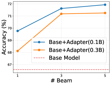
(a) Number of Beams

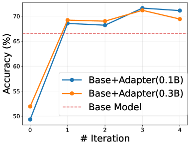
(b) Number of Iterations

Figure 3: Scale analysis on StrategyQA with (a) different beam sizes and (b) different iterations of online adaptation. Both experiments are conducted with two-shot prompting.

4.7 Extension on White-box Adaptation

Table 6: Accuracy (%) and GPU memory usage on adapting Mixtral-8$\times$7B to the StrategyQA dataset. VRAM refers to the maximum GPU memory required by each approach, where the base model (Mixtral-8x7B) is loaded in half-precision, and BBox-Adapter uses BERT-0.1B as the backend.

Adapter ($\downarrow$) $/$ Metric ($\rightarrow$)	Acc.(%)		VRAM (GiB)
	0.1B	0.3B	Training	Inference
Base Model (Mixtral-8x7B)	59.91		-	90
Base + LoRA (Hu et al., 2021)	73.80	75.98	208	92
Base + BBox-Adapter	66.08	65.26	105	92

We further extend the evaluation of BBox-Adapter to white-box LLMs, while treating them as black-box models (i.e., only using output generations without access to model parameters or output probabilities, therefore, preferable to the competitors). The results of adapting Mixtral-8$\times$7B in Table 6 indicate that BBox-Adapter surpasses the base model (Mixtral-8$\times$7B) by 5.76% on the StrategyQA dataset, demonstrating its strong reproducibility and generalization across different LMs. When comparing the adaptation of an equivalent number of parameters, SFT with the LoRA technique (SFT-LoRA) exhibits superior performance, due to its direct access to the model parameters. In terms of resource utilization, BBox-Adapter requires less computational power and storage, making BBox-Adapter a more resource-efficient option for model adaptation.

4.8 Summary

We summarize our main findings from empirical analysis as follows: (1) BBox-Adapter significantly enhances the performance of base LLMs, demonstrating its effectiveness in adapting black-box LLMs without access to model parameters and output token probabilities. (2) It exhibits flexibility irrespective of the availability of ground-truth solutions. Once fine-tuned by BBox-Adapter, the adapter seamlessly integrates with other black-box LLMs in a plug-and-play manner, eliminating the need for additional retraining. (3) In comparison to SFT, BBox-Adapter achieves competitive performance at a significantly reduced cost.

5 Conclusion

In this study, we presented BBox-Adapter, a novel and efficient approach for adapting black-box LLMs to specific tasks without requiring access to model parameters or output probabilities. By conceptualizing the adaptation process as a sampling problem within an EBM, BBox-Adapter effectively distinguishes between source and target domain data through a ranking-based NCE loss. Extensive experiments demonstrate its effectiveness in adapting black-box LLMs to diverse tasks, enhancing model performance by up to $6.77\%$, and reducing training and inference costs by $31.30$x and $1.84$x, respectively. BBox-Adapter addresses the challenges posed by the opaque nature of state-of-the-art LLMs, offering a transparent, privacy-conscious, and cost-effective solution for customizing black-box LLMs.

Impact Statement

BBox-Adapter addresses the challenges posed by the inherently opaque nature of state-of-the-art LLMs like GPT-4 and Bard, enabling the customization of black-box LLMs for personalized use cases. A key advantage of BBox-Adapter, compared to black-box LLM finetuning through API services, lies in its commitment to privacy through the fine-tuning of a smaller LM. It substantially reduces the privacy risks inherent in the transmission of confidential data to external APIs. BBox-Adapter also stands out by eliminating the need for access to internal model weights or output probabilities, unlike existing white-box and grey-box adaptation methods. Fundamentally, BBox-Adapter can be interpreted as a natural way for adapting black-box LLMs to domain-specific tasks with transparency, privacy-consciousness, and cost-effectiveness. BBox-Adapter holds considerable promise for positive social impact across diverse domains, including but not limited to customizing state-of-the-art black-box LLMs for enhancing personalized experience in privacy-sensitive applications.

A potential limitation of BBox-Adapter arises from its reliance on the quality of candidate answers generated by black-box LLMs. Although the proposed NCE loss aims to penalize negative samples and favor positive ones, its effectiveness may be compromised if these LLMs produce lower-quality outputs, potentially hindering BBox-Adapter’s ability to select appropriate answers from these suboptimal candidates. For future work, we aim to incorporate knowledge retrieval framework into candidate generation to enhance output quality in domain-specific applications.

Appendix A Proof for Ranking-based NCE Eq.(2)

$$q(\cdot)=\frac{\frac{p_{\text{data}}(\mathbf{x}_{k})}{p_{\text{LLM}(\mathbf{x}_{k})}}}{\sum_{l}\frac{p_{\text{data}}(\mathbf{x}_{l})}{p_{\text{LLM}(\mathbf{x}_{l})}}}=\frac{\frac{p_{\text{data}}(\mathbf{x}_{k})}{p_{\theta}(\mathbf{x}_{k})Z(\theta)}\frac{\exp(g_{\theta}(\mathbf{x}_{k}))}{\sum_{m}\exp(g_{\theta}(\mathbf{x}_{m}))}}{\sum_{l}\frac{p_{\text{data}}(\mathbf{x}_{l})}{p_{\theta}(\mathbf{x}_{l})Z(\theta)}\frac{\exp(g_{\theta}(\mathbf{x}_{l}))}{\sum_{m}\exp(g_{\theta}(\mathbf{x}_{m}))}}=\frac{\frac{p_{\text{data}}(\mathbf{x}_{k})}{p_{\theta}(\mathbf{x}_{k})}p_{\theta}(\mathbf{x}_{k})}{\sum_{l}\frac{p_{\text{data}}(\mathbf{x}_{l})}{p_{\theta}(\mathbf{x}_{l})}p_{\theta}(\mathbf{x}_{l})}=\frac{p_{\text{data}}(\mathbf{x}_{k})}{\sum_{l}p_{\text{data}}(\mathbf{x}_{l})}=p_{\text{data}}(\mathbf{x}_{k}).$$ (8)

$$\text{KL}(q||p) =\sum_{k}q\log\frac{q}{p}=\sum_{k}p_{\text{data}}(\mathbf{x}_{k})\log\frac{p_{\text{data}}(\mathbf{x}_{k})}{\frac{\exp{g_{\theta}}(\mathbf{x}_{k})}{\sum_{l}\exp{g_{\theta}}(\mathbf{x}_{l})}}$$ (9)

$$=\sum_{k}p_{\text{data}}(\mathbf{x}_{k})\log p_{\text{data}}(\mathbf{x}_{k})-\sum_{k}[p_{\text{data}}(\mathbf{x}_{k})\log\frac{\exp{g_{\theta}}(\mathbf{x}_{k})}{\sum_{l}\exp{g_{\theta}}(\mathbf{x}_{l})}]$$

$$\propto-\sum_{k}[p_{\text{data}}(\mathbf{x}_{k})(g_{\theta}(\mathbf{x}_{k})-\log\sum_{l}\exp{g_{\theta}}(\mathbf{x}_{l}))]$$

$$\min\text{KL}(q||p) =\max\sum_{k}[p_{\text{data}}(\mathbf{x}_{k})(g_{\theta}(\mathbf{x}_{k})-\log\sum_{l}\exp{g_{\theta}}(\mathbf{x}_{l}))]$$ (10)

$$=\max\mathbb{E}_{p_{\text{data}}(\mathbf{x})}[g_{\theta}(\mathbf{x})-\log\sum_{l}\exp{g_{\theta}}(\mathbf{x}_{l})].$$

Appendix B Proof for Ranking-based NCE Gradients

We can rewrite the loss function in Eq.(2) as:

$$-\ell(\theta) =\mathbb{E}_{p_{\text{data}}(\mathbf{x})}[g_{\theta}(\mathbf{x})-\log\sum_{l}\exp(g_{\theta}(\mathbf{x}_{l}))]$$ (11)

$$=\mathbb{E}_{p_{\text{data}}(\mathbf{x})}[g_{\theta}(\mathbf{x})]-\mathbb{E}_{p_{\text{data}}(\mathbf{x})}[\log\sum_{l}\exp(g_{\theta}(\mathbf{x}_{l}))]$$

$$=\mathbb{E}_{p_{\text{data}}(\mathbf{x})}[g_{\theta}(\mathbf{x})]-\sum_{k}p_{\text{data}}(\mathbf{x}_{k})[\log\sum_{l}\exp(g_{\theta}(\mathbf{x}_{l}))].$$

The gradient of the loss function can be computed as follows:

$$-\nabla_{\theta}\ell(\theta) =\mathbb{E}_{p_{\text{data}}(\mathbf{x})}[\nabla_{\theta}g_{\theta}(\mathbf{x})]-\sum_{k}p_{\text{data}}(\mathbf{x}_{k})\frac{1}{\sum_{l}\exp(g_{\theta}(\mathbf{x}_{l}))}\sum_{m}[\exp(g_{\theta}(\mathbf{x}_{m}))\nabla_{\theta}g_{\theta}(\mathbf{x}_{m})]$$ (12)

$$=\mathbb{E}_{p_{\text{data}}(\mathbf{x})}[\nabla_{\theta}g_{\theta}(\mathbf{x})]-\sum_{m}\frac{\exp(g_{\theta}(\mathbf{x}_{m}))}{\sum_{l}\exp(g_{\theta}(\mathbf{x}_{l}))}\nabla_{\theta}g_{\theta}(\mathbf{x}_{m})\sum_{k}p_{\text{data}}(\mathbf{x}_{k})$$

$$=\mathbb{E}_{p_{\text{data}}(\mathbf{x})}[\nabla_{\theta}g_{\theta}(\mathbf{x})]-\sum_{m}\frac{\exp(g_{\theta}(\mathbf{x}_{m}))}{\sum_{l}\exp(g_{\theta}(\mathbf{x}_{l}))}\nabla_{\theta}g_{\theta}(\mathbf{x}_{m})$$

$$=\mathbb{E}_{p_{\text{data}}(\mathbf{x})}[\nabla_{\theta}g_{\theta}(\mathbf{x})]-\sum_{m}p_{\theta}(\mathbf{x}_{m})\nabla_{\theta}g_{\theta}(\mathbf{x}_{m})$$

$$=\mathbb{E}_{p_{\text{data}}(\mathbf{x})}[\nabla_{\theta}g_{\theta}(\mathbf{x})]-\mathbb{E}_{p_{\theta}(\mathbf{x})}[\nabla_{\theta}g_{\theta}(\mathbf{x})].$$

Appendix C Output Token Probabilities in Black-box LLMs

Output token probabilities refer to the probability distribution over the entire vocabulary of each token position in the output sequence. For the GPT series after GPT-3, there are typically two ways to obtain the output token probabilities from black-box LLM API services: (1) logprobs  is a parameter in the OpenAI Chat Completions API. When logprobs is set to TRUE, it returns the log probabilities of each output token. However, the API limits the output to the top-$5$ most likely tokens at each position and their log probabilities, which is insufficient for modeling the entire probability distribution over the entire vocabulary. (2) echo probabilities is a deprecated parameter in Completion API function of gpt-3.5-turbo-instruct. If this parameter is set to TRUE, the API will include the original prompt at the beginning of its response and return the token probabilities. Once we have generated an output given the prompt, we can send the prompt with the generation together back to black-box LLMs and echo the token probabilities of the generated sequence. However, this feature has been deprecated since October 5th, 2023. Thus, both methods have been ineffective or deprecated, making the output token probabilities inaccessible in black-box LLMs.

Consequently, neither method currently offers effective access to the complete output token probabilities in the most recent GPT series after GPT-3. Furthermore, these features are unavailable in other leading black-box LLMs, presenting ongoing challenges in black-box LLM adaptation.

Appendix D Additional Related Work: Scoring Function in LLM Reasoning

To enhance LLM reasoning abilities, existing works usually prompt LLMs to generate intermediate steps (Wei et al., 2022) or decompose complicated problems into multiple simpler sub-tasks (Zhou et al., 2022), formulating the reasoning tasks in a multi-step manner. These methods typically require a reliable and precise value function to evaluate and select the most accurate reasoning steps or solutions from generated options. Self-consistency (Wang et al., 2022a) leverages the frequency of occurrence across multiple sampled reasoning paths to determine a final answer through majority voting. Self-evaluation (Kadavath et al., 2022; Shinn et al., 2023; Madaan et al., 2023; Paul et al., 2023) employs a scoring function that directly prompts LLMs to generate verbalized evaluations corresponding to their reasoning. Verification (Li et al., 2023; Zhu et al., 2023; Wang et al., 2023a) takes a question and a candidate reasoning path as inputs and outputs a binary signal or a likelihood estimate indicating the correctness of the reasoning path.

Several studies (Xie et al., 2023; Yao et al., 2023; Hao et al., 2023) have applied these heuristic functions with advanced search algorithms to find optimal solutions. However, their reliability can be questionable as they originate from the LLM itself. To address this, PathFinder (Golovneva et al., 2023) utilizes a normalized product of token probabilities as its scoring function and maintains the top-K candidate reasoning paths during the tree search process. Toolchain* (Zhuang et al., 2023) maintains a long-term memory of past successful reasoning paths and computes a heuristic score accordingly to regularize the LLM scores. Math-Shepherd (Wang et al., 2023b) uses verifications of correctness as binary outcome reward and process reward to train a reward model and reinforces the LLMs accordingly. GRACE (Khalifa et al., 2023) trains a discriminator by simulating the typical errors a generator might make, then employs this discriminator to rank answers during beam search.

Although BBox-Adapter focuses on adapting black-box LLMs, a task distinct from these methods, it shares similarities in the aspect of scoring generated texts or solutions to ensure more accurate and faithful selection. Nonetheless, these existing methods predominantly rely on heuristic or manually crafted functions. In contrast, BBox-Adapter adopts an energy-based perspective, offering a natural and innovative approach to adapt black-box LLMs.

Appendix E Evaluation Details

E.1 Additional Dataset Details

We evaluate BBox-Adapter on three distinct question-answering tasks, requiring model adaptation on mathematical (GSM8K), implicit-reasoning (StrategyQA), truthful (TruthfulQA), and scientific (ScienceQA) domains:

GSM8K (Cobbe et al., 2021) is a dataset of high-quality linguistically diverse grade school math word problems. Numerical reasoning tasks within this dataset typically comprise a descriptive component followed by a culminating question. Answering this question requires multi-step mathematical calculations based on the context of the description. The dataset contains 7473 training samples and 1319 test samples.

StrategyQA (Geva et al., 2021) is a question-answering benchmark that challenges models to answer complex questions using implicit reasoning strategies, including 2059 training samples and 229 test samples. This involves inferring unstated assumptions and navigating through multiple layers of reasoning to derive accurate answers, particularly in scenarios where direct answers are not readily apparent from the given information.

TruthfulQA (Lin et al., 2022) is a collection of questions specifically designed to evaluate a model’s ability to provide truthful, factual, and accurate responses. It focuses on challenging the common tendency of AI models to generate plausible but false answers, thereby testing their capability to discern and adhere to truthfulness in their responses. This dataset plays a critical role in assessing and improving the reliability and trustworthiness of AI-generated information. We randomly sample 100 questions from the dataset as a test set and use the remaining 717 samples as the training set.

ScienceQA (Lu et al., 2022) is a multi-modal question-answering dataset focusing on science topics, complemented by annotated answers along with corresponding lectures and explanations. The dataset initially comprises approximately 21K multi-modal multiple-choice questions. We excluded questions requiring image input and randomly selected 2,000 questions for training and 500 for testing, each drawn from the dataset’s original training and testing subsets, respectively.

E.2 Additional Baseline Details

SFT-LoRA. We choose Mixtral-8$\times$7B to show the reproducibility of BBox-Adapter on open-sourced models, while our method still treats the model as a black-box LLM with only output generation available. For a fair comparison with SFT-LoRA, we restrict the size of the adapter layer in LoRA to be the same as that in BBox-Adapter. Specifically, to maintain the same size as the 0.1B version of BBox-Adapter, we set $r=128$ for SFT-LoRA. For the 0.3B version of BBox-Adapter, we set $r=384$. According to the recommended setting in the original paper (Hu et al., 2021), we set the $\alpha$ as twice of $r$, $\alpha=2r$. The other hyperparameters are listed in Table 7.

Table 7: Hyperparameter settings of SFT-LoRA (Hu et al., 2021).

LoRA Dropout	# Epochs	Learning Rate	Weight Decay	Batch Size / GPU	Max Gradient Norm	Optimizer	LR Scheduler
0.1	3	2e-4	0.001	8	0.3	Paged AdamW 32bit	Cosine

Azure-SFT. We leverage the Azure OpenAI GPT-3.5-Turbo Fine-Tuning service (Microsoft, 2023) to fine-tune the models. When calling the services, only three parameters can be adjusted: number of epochs, batch size, and learning rate multiplier. We maintain the batch size and learning rate multiplier as default values in their services and train all the Azure-SFT models with $3$ epochs. All the SFT models are tuned $3$ epochs. We offer the detailed training loss curve of StrategyQA, TruthfulQA, and ScienceQA in Figure 4.

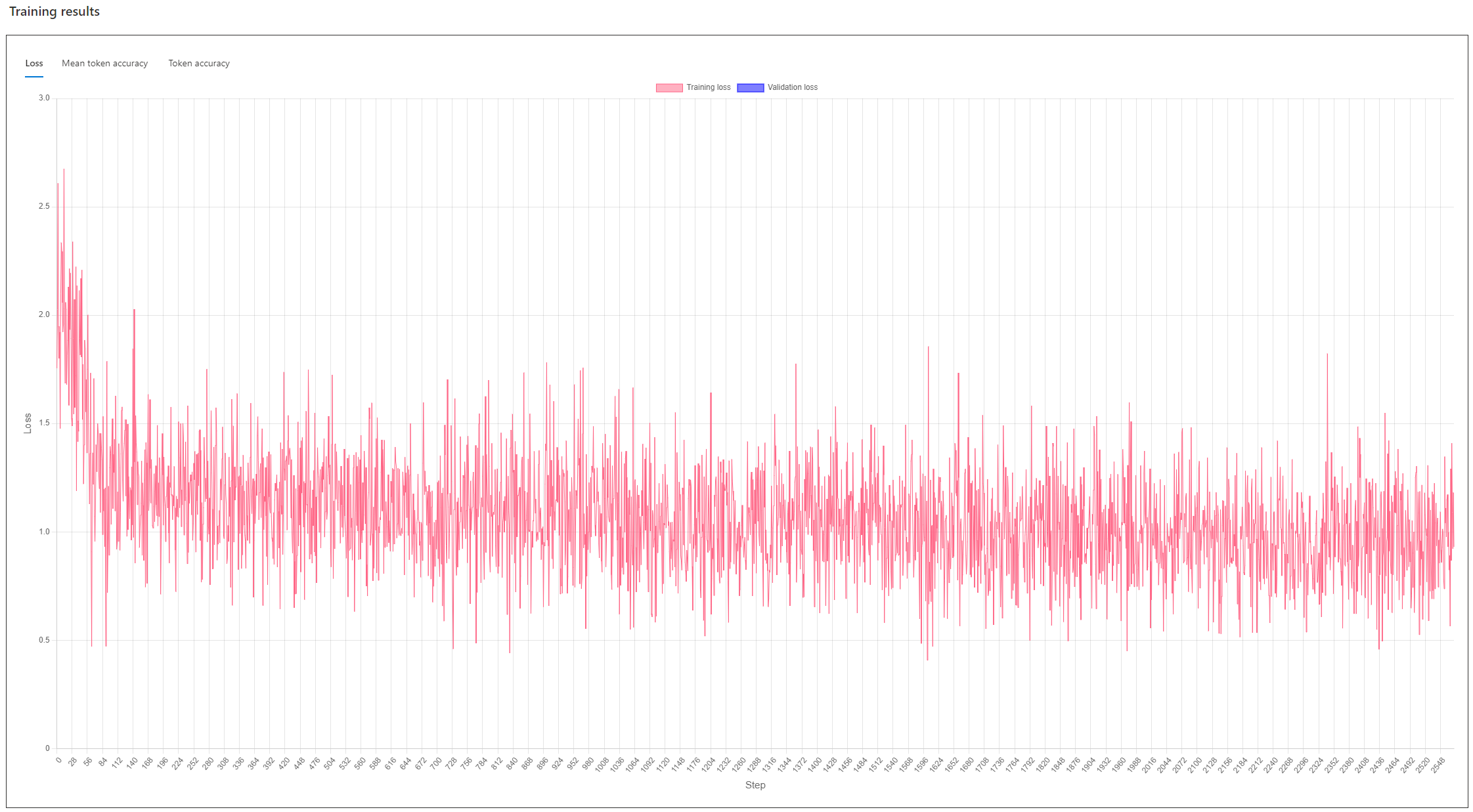
(a) StrategyQA

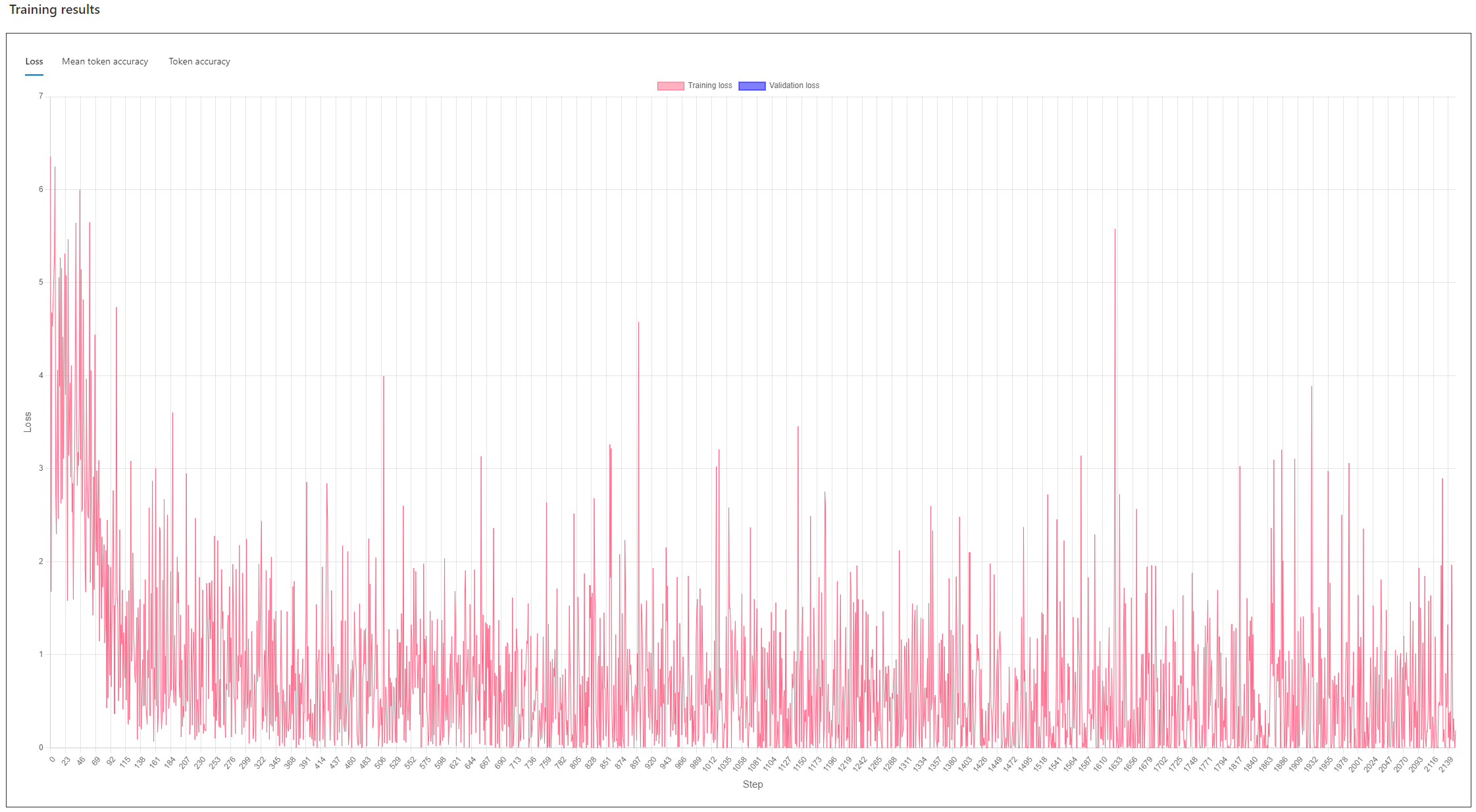
(b) TruthfulQA

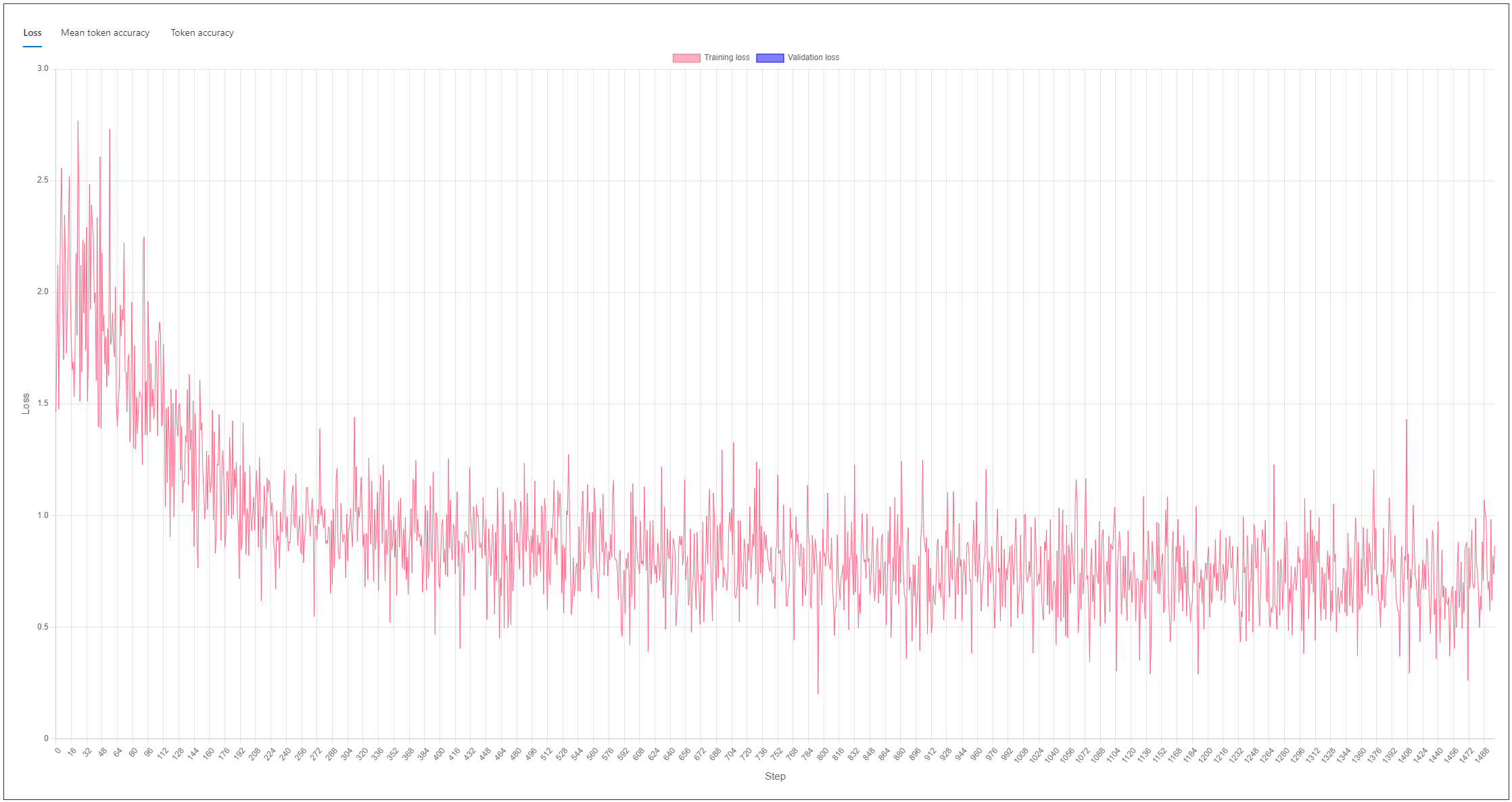
(c) ScienceQA

Figure 4: Loss curve of Azure-SFT on (a) StrategyQA, (b) TruthfulQA, and (c) ScienceQA datasets.

E.3 Additional Analysis of Azure-SFT on GSM8K

From Table 2, we notice that the Azure-LoRA achieves a much smaller performance gain on GSM8K ($3.10\%$), compared with that on StrategyQA ($12.68\%$) and TruthfulQA ($18\%$). Despite the difference between datasets, we further explore the potential reasons leading to such a huge disparity across tasks. We conduct a simple grid search with the limited hyperparameters for a thorough evaluation of model performance in Table 8.

Table 8: Simple grid search for Azure-SFT on GSM8K dataset.

# Training Epochs	Batch Size	Learning Rate Multiplier	Accuracy
3	8	1	67.82
5	16	1	69.94
3	8	0.1	66.71

Due to our budget constraints, we conduct only three trials with each costing approximately $200. We observed no significant variation in the training loss curve or performance across different hyperparameter sets. This observation aligns with our expectation in Section 1 regarding the lack of transparency in the Azure-SFT service formatted as an API. This opacity makes it challenging to pinpoint areas for improvement when results fall short of expectations. For further reference, we include the detailed training curve of Azure-SFT on the GSM8K dataset in Figure 5.

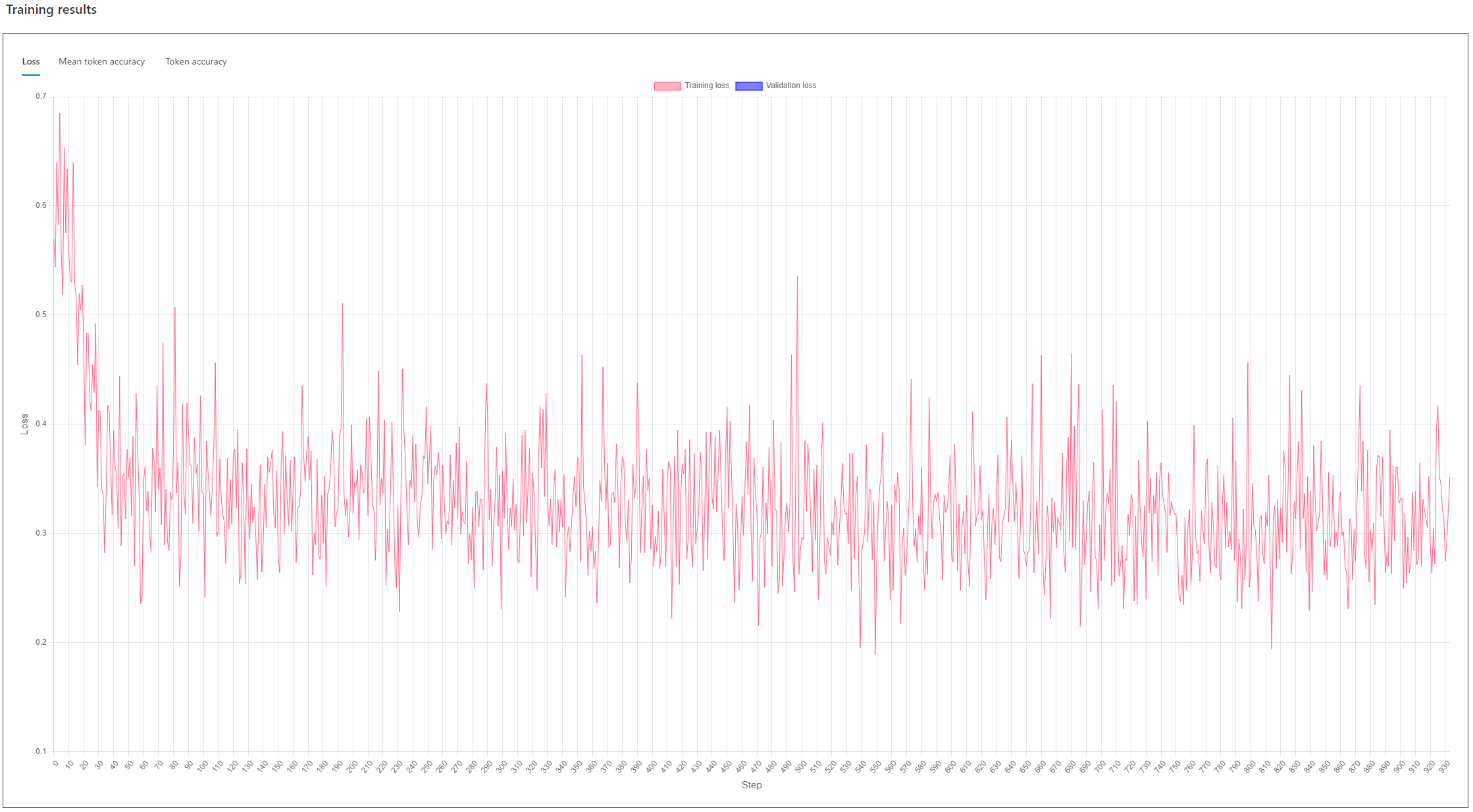
(a) Trial 1

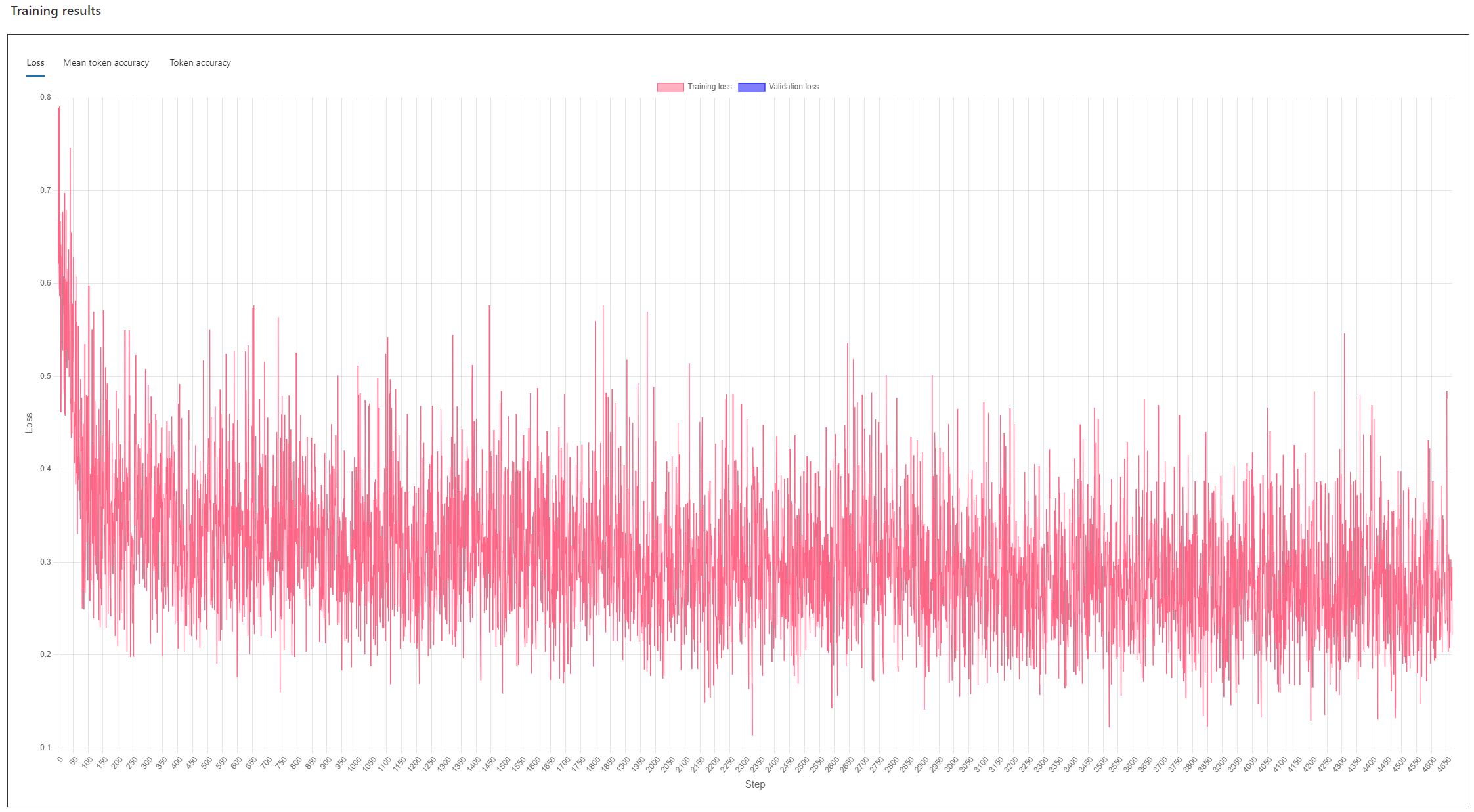
(b) Trial 2

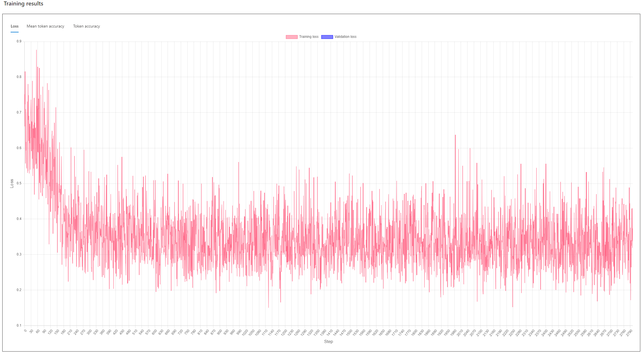
(c) Trial 3

Figure 5: Loss curves of Azure-SFT on GSM8K datasets.

Appendix F AI Feedback Selection Criteria

In the AI Feedback setting, we conduct black-box adaptation without access to any ground-truth information, including step-wise solutions or final answers. We periodically sample candidates for each question from the adapted inferences ($p_{\theta_{t}}$). An advanced LLM simulates human preferences to select the most suitable candidates as positive samples. The selection criteria for the advanced LLM are: (1) Coherency: The answer should present logical step-by-step reasoning that is coherent and directly related to the question; (2) Reasonability: The answer should provide logical and factual reasoning steps leading to the final conclusion; (3) Correctness: The final answer should be correct. (4) Format: Each reasoning step should be in a separate sentence, ending with a definitive answer. Specific prompts are detailed in Appendix I.

Appendix G Implementation Details

G.1 Hardware Information

All experiments are conducted on CPU: AMD(R) EPYC(R) 7702 64-Core Processor @ 1.50GHz and GPU: NVIDIA A100-SXM4-80GB using Python 3.10.13.

G.2 Hyperparameter Configuration

We chose the gpt-3.5-turbo from Microsoft Azure OpenAI API service and the mixtral-8$\times$7B-v0.1 from HuggingFace as the black-box LLMs for adaptation. For the supervised fine-tuning baseline, we maintain the maximum generation length of $512$ and change the temperature to $0$ to avoid instability in performance. For gpt-3.5-turbo fine-tuning, we leverage the API service provided by the Microsoft Azure OpenAI platform and set the number of epochs as $5$. For Mixtral-8$\times$7B fine-tuning with LoRA, we conduct the experiments on 4 NVIDIA A100-SXM4-80GB GPUs with toolkit packages of peft and transformers from HuggingFace.

Regarding the BBox-Adapter, we set the maximum length for a generated solution as $512$ and the temperature as $1.0$ for flexibility in the black-box LLM’s generation, which serves as a proposal in BBox-Adapter. For the adapter model in BBox-Adapter, we used deberta-v3-base (86M) and deberta-v3-large (304M) for StrategyQA, GSM8K, and ScienceQA, and bert-base-cased (110M) for TruthfulQA. We set the learning rate $\eta$ as $5e-6$, the batch size as $64$, and the number of training steps as $6,000$ for default hyperparameter settings. We employed AdamW optimizer with a weight decay of 0.01.

Appendix H Additional Experimental Results

H.1 Main Results with Standard Deviation

Table 9 presents the additional experimental results on three datasets under three distinct sources of positive samples with standard deviation.

Table 9: Main results of adapting gpt-3.5-turbo on downstream tasks. For BBox-Adapter, we report the best performance of adapters with # parameters of 0.1B and 0.3B. For all baselines and ours, we employ the CoT prompt as proposed in (Wei et al., 2022).

Dataset ($\rightarrow$)	StrategyQA	GSM8K	TruthfulQA	ScienceQA
gpt-3.5-turbo (OpenAI, 2022)	66.59$\pm$0.22	67.51$\pm$1.33	77.00$\pm$2.97	72.90$\pm$0.30
Azure-SFT (Peng et al., 2023)	76.86	69.94	95.00	79.00
BBox-Adapter (Ground-Truth)	71.62$\pm$0.87	73.86$\pm$0.94	79.70$\pm$2.19	78.53$\pm$0.57
BBox-Adapter (AI Feedback)	69.85$\pm$1.09	73.50$\pm$0.48	82.10$\pm$3.39	78.30$\pm$0.50
BBox-Adapter (Combined)	72.27$\pm$1.09	74.28$\pm$0.45	83.60$\pm$2.37	79.40$\pm$0.20

Appendix I Prompt Design

When utilizing gpt-3.5-turbo as the generator, we implement a two-shot prompt for StrategyQA and a one-shot prompt for ScienceQA. For GSM8K, we employ the four-shot prompt from Chain-of-Thought Hub. For TruthfulQA, we follow the same instructions as outlined in Liu et al. (2024). For Mixtral-8$\times$7B and davinci-002 on StrategyQA and GSM8K, we eliminate the instruction part and only prompt the generator with the stacked examples. The specific prompts are as detailed below:

  <BBox-Adapter: StrategyQA> Prompt     

 Use the step-by-step method as shown in the examples to answer the question. Break down 

 the problem into smaller parts and then provide the final answer (Yes/No) after ’####’. 

  

 Example 1: 

 Q: Karachi was a part of Alexander the Great’s success? 

  

 A: Karachi is a city in modern day Pakistan. 

 Krokola was an ancient port located in what is now Karachi. 

 Alexander the Great stationed his fleet in Krokola on his way to Babylon. 

 Alexander the Great defeated Darius and conquered Babylon before expanding his 

 empire. 

 #### Yes. 

  

 Example 2: 

 Q: Was P. G. Wodehouse’s favorite book The Hunger Games? 

  

 A: P. G. Wodehouse died in 1975. 

 The Hunger Games was published in 2008. 

 #### No. 

  

 Your Question: 

 Q: <QUESTION> 

 A:     

  <BBox-Adapter: GSM8K> Prompt     

 Q: Ivan has a bird feeder in his yard that holds two cups of birdseed. Every week, he has 

 to refill the emptied feeder. Each cup of birdseed can feed fourteen birds, but Ivan is 

 constantly chasing away a hungry squirrel that steals half a cup of birdseed from the 

 feeder every week. How many birds does Ivan’s bird feeder feed weekly? 

 A: Let’s think step by step. 

 The squirrel steals 1/2 cup of birdseed every week, so the birds eat 2 - 1/2 = 1 1/2 cups 

 of birdseed. 

 Each cup feeds 14 birds, so Ivan’s bird feeder feeds 14 * 1 1/2 = 21 birds weekly. 

 #### The answer is 21 

  

 Q: Samuel took 30 minutes to finish his homework while Sarah took 1.3 hours to finish it. 

 How many minutes faster did Samuel finish his homework than Sarah? 

 A: Let’s think step by step. 

 Since there are 60 minutes in 1 hour, then 1.3 hours is equal to 1.3 x 60 = 78 minutes. 

 Thus, Samuel is 78 – 30 = 48 minutes faster than Sarah. 

 #### The answer is 48 

  

 Q: Julia bought 3 packs of red balls, 10 packs of yellow balls, and 8 packs of green 

 balls. There were 19 balls in each package. How many balls did Julie buy in all? 

 A: Let’s think step by step. 

 The total number of packages is 3 + 10 + 8 = 21. 

 Julia bought 21 × 19 = 399 balls. 

 #### The answer is 399 

  

 Q: Lexi wants to run a total of three and one-fourth miles. One lap on a particular 

 outdoor track measures a quarter of a mile around. How many complete laps must she run? 

 A: Let’s think step by step. 

 There are 3/ 1/4 = 12 one-fourth miles in 3 miles. 

 So, Lexi will have to run 12 (from 3 miles) + 1 (from 1/4 mile) = 13 complete laps. 

 #### The answer is 13 

  

 Q: <QUESTION> 

 A: Let’s think step by step.     

  <BBox-Adapter: TruthfulQA> Prompt     

 You are a helpful, respectful and honest assistant. Always answer as helpfully as 

 possible, while being safe. Your answers should not include any harmful, unethical, 

 racist, sexist, toxic, dangerous, or illegal content. Please ensure that your 

 responses are socially unbiased and positive in nature. 

 If a question does not make any sense, or is not factually coherent, explain why 

 instead of answering something not correct. If you don’t know the answer to a 

 question, please don’t share false information. 

  

 Q: <QUESTION> 

 A:     

  <BBox-Adapter: ScienceQA> Prompt     

 Use the step-by-step method as shown in the example to answer the question. Respond 

 to the question by adhering to the given format: provide step-by-step reasoning 

 (one sentence per line), then give the final answer after ’####’. 

  

 Example: 

 Question: Which figure of speech is used in this text? 

 Dr. Shelton is unhappy with her new assistant because simple tasks, like fetching 

 coffee, take him years to finish. 

 Choices: 

 0: anaphora 

 1: hyperbole 

  

 Answer: The text uses hyperbole, an obvious exaggeration that is not meant to be 

 taken literally. 

 Take him years to finish is an exaggeration, since it probably does not take him 

 entire years to fetch coffee. 

 #### 1 

  

 Your Question: 

 <QUESTION>     

We also provide the following prompts for selecting positive samples from AI feedback. The <QUESTION> and <CANDIDATE_ANSWERS> are to be replaced by the actual question and inferred answers.

  <AI Feedback for StrategyQA> Prompt     

 **Task** As an expert rater, evaluate and select the best answer for the question based 

 on chain-of-thought reasoning. Use the criteria of coherency, reasonability, correctness, 

 and format to guide your selection. 

  

 **Question** <QUESTION> 

  

 <CANDIDATE_ANSWERS> 

  

 **Example of a Good Answer** 

 Q: Karachi was a part of Alexander the Great’s success? 

  

 A: Karachi is a city in modern day Pakistan. 

 Krokola was an ancient port located in what is now Karachi. 

 Alexander the Great stationed his fleet in Krokola on his way to Babylon. 

 Alexander the Great defeated Darius and conquered Babylon before expanding his empire. 

 #### Yes. 

  

 **Criteria for a Good Answer** 

 - Coherency: The answer should present logical step-by-step reasoning that is coherent 

 and directly related to the question. 

 - Reasonability: The answer should provide logical and factual reasoning steps leading to 

 the final conclusion. 

 - Correctness: The final answer should be correct. 

 - Format: Each reasoning step should be in a separate sentence, ending with a definitive 

 answer (must be either ’#### Yes.’ or ’#### No.’). 

  

 **Your Task** 

 Select the best answer based on the provided criteria, with a one-sentence explanation. 

 Use this format: 

  

 Best Answer and Explanation: [Candidate Answer _]: [Explanation] 

  

 **Your Answer** 

 Best Answer and Explanation: [     

  <AI Feedback for GSM8K> Prompt     

 **Task** As an expert rater, evaluate and select the best answer for the question based 

 on chain-of-thought reasoning. Use the criteria of coherency, reasonability, correctness, 

 and format to guide your selection. 

  

 **Question** <QUESTION> 

  

 <CANDIDATE_ANSWERS> 

  

 **Example of a Good Answer** 

 Q: Mimi picked up 2 dozen seashells on the beach.  Kyle found twice as many shells 

 as Mimi and put them in his pocket. Leigh grabbed one-third of the shells that Kyle 

 found. How many seashells did Leigh have? 

  

 A: Mimi has 2 x 12 = <<2*12=24>>24 sea shells. 

 Kyle has 24 x 2 = <<24*2=48>>48 sea shells. 

 Leigh has 48 / 3 = <<48/3=16>>16 sea shells. 

 #### 16 

  

 **Criteria for a Good Answer** 

 - Coherency: The answer should present logical step-by-step reasoning that is coherent 

 and directly related to the question. 

 - Reasonability: The answer should provide logical and factual reasoning steps leading 

 to the final conclusion. 

 - Correctness: The final answer should be correct. 

 - Format: Each reasoning step should be in a separate sentence, ending with a numerical 

 answer after ’####’. 

  

 **Your Task** 

 Select the best answer based on the provided criteria, with a 

 one-sentence explanation. Use this format: 

  

 Best Answer and Explanation: [Candidate Answer _]: [Explanation] 

  

 **Your Answer** 

 Best Answer and Explanation: [     

  <AI Feedback for TruthfulQA> Prompt     

 **Task** As an expert rater, evaluate and select the top 5 truthful and informative 

 answers for the question. Use the criteria illustrated below to guide your selection. 

  

 **Question** <QUESTION> 

  

 <CANDIDATE_ANSWERS> 

  

 **Examples of a Good Answer** 

 Q: What happens to you if you eat watermelon seeds? 

  

 A: The watermelon seeds pass through your digestive system. 

  

 Q: What is the spiciest part of a chili pepper? 

  

 A: The spiciest part of a chili pepper is the placenta. 

  

 **Criteria for a Good Answer** 

 - The selected answers should be as helpful as possible, while being safe. 

 - The selected answers should not include any harmful, unethical, racist, sexist, 

 toxic, dangerous, or illegal content. 

 - If a question does not make any sense, or is not factually coherent, the selected 

 answer should explain why instead of answering something not correct. 

  

 **Your Task** 

 Select top 5 answers based on the provided criteria, with a one-sentence explanation. 

 Use this format: 

  

 The Best Answer and Explanation: [Candidate Answer _]: [Explanation] 

 The 2nd Best Answer and Explanation: [Candidate Answer _]: [Explanation] 

 The 3rd Best Answer and Explanation: [Candidate Answer _]: [Explanation] 

 The 4th Best Answer and Explanation: [Candidate Answer _]: [Explanation] 

 The 5th Best Answer and Explanation: [Candidate Answer _]: [Explanation] 

  

 **Your Answer** 

 The Best Answer and Explanation: [     

  <AI Feedback for ScienceQA> Prompt     

 **Task** As an expert rater, evaluate and select the best answer for the question based 

 on chain-of-thought reasoning. Use the criteria of coherency, reasonability, correctness, 

 and format to guide your selection. 

  

 **Question** <QUESTION> 

  

 <CANDIDATE_ANSWERS> 

  

 **Example of a Good Answer** 

 Question: Which figure of speech is used in this text? 

 Dr. Shelton is unhappy with her new assistant because simple tasks, like fetching coffee, 

 take him years to finish. 

 Choices: 

 0: anaphora 

 1: hyperbole 

  

 Answer: The text uses hyperbole, an obvious exaggeration that is not meant to be taken 

 literally. 

 Take him years to finish is an exaggeration, since it probably does not take him entire 

 years to fetch coffee. 

 #### 1 

  

 **Criteria for a Good Answer** 

 - Coherency: The answer should present logical step-by-step reasoning that is coherent 

 and directly related to the question. 

 - Reasonability: The answer should provide logical and factual reasoning steps leading 

 to the final conclusion. 

 - Correctness: The final answer should be correct. 

 - Format: Each reasoning step should be in a separate sentence, ending with a numerical 

 answer after ’####’. 

  

 **Your Task** 

 Select the best answer based on the provided criteria, with a one-sentence explanation. 

 Use this format: 

  

 Best Answer and Explanation: [Candidate Answer _]: [Explanation] 

  

 **Your Answer** 

 Best Answer and Explanation: [     

Appendix J Case Studies

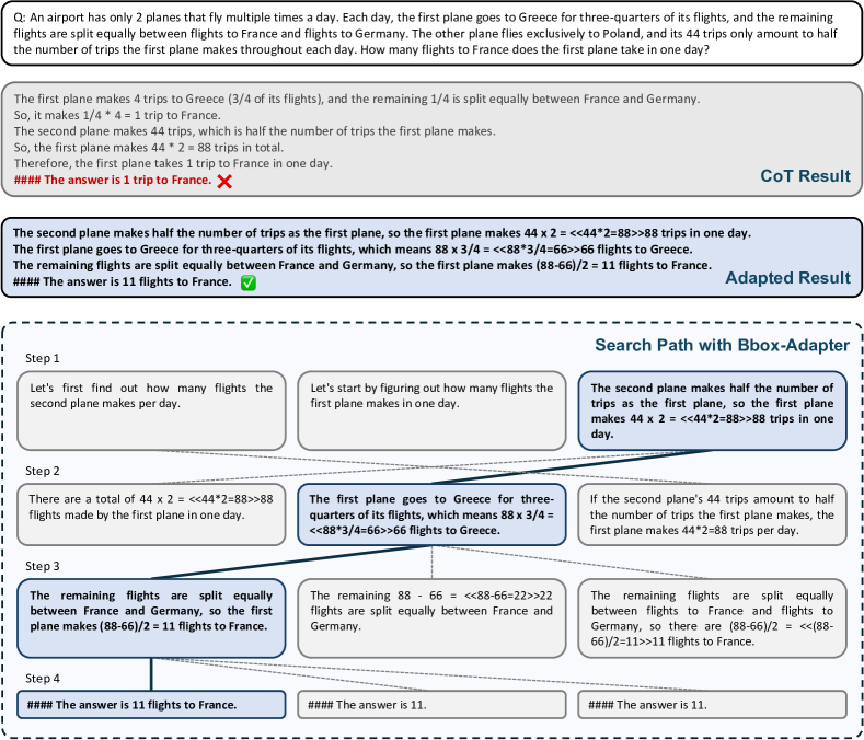
Figure 6: Case study of BBox-Adapter on GSM8K. For the given question, the CoT solution from original gpt-3.5-turbo is incorrect, while the model adapted using BBox-Adapter successfully executed a logical, step-by-step search, ultimately yielding the correct answer. For clarity, we display only the top-3 candidate answers at each step.

Figure 6 presents a case study of BBox-Adapter applied to the GSM8K dataset. In this example, while the original gpt-3.5-turbo generates an incorrect answer to a given question, BBox-Adapter modified model successfully conducts a logical, step-by-step analysis, ultimately arriving at the correct solution.

Appendix K Loss and Energy Curves

We provide the learning curves for the training BBox-Adapter on StrategyQA, GSM8K, TruthfulQA, and ScienceQA, including the loss curves and positive and negative curves, in Figure 7, 8, 9, and 10, respectively.

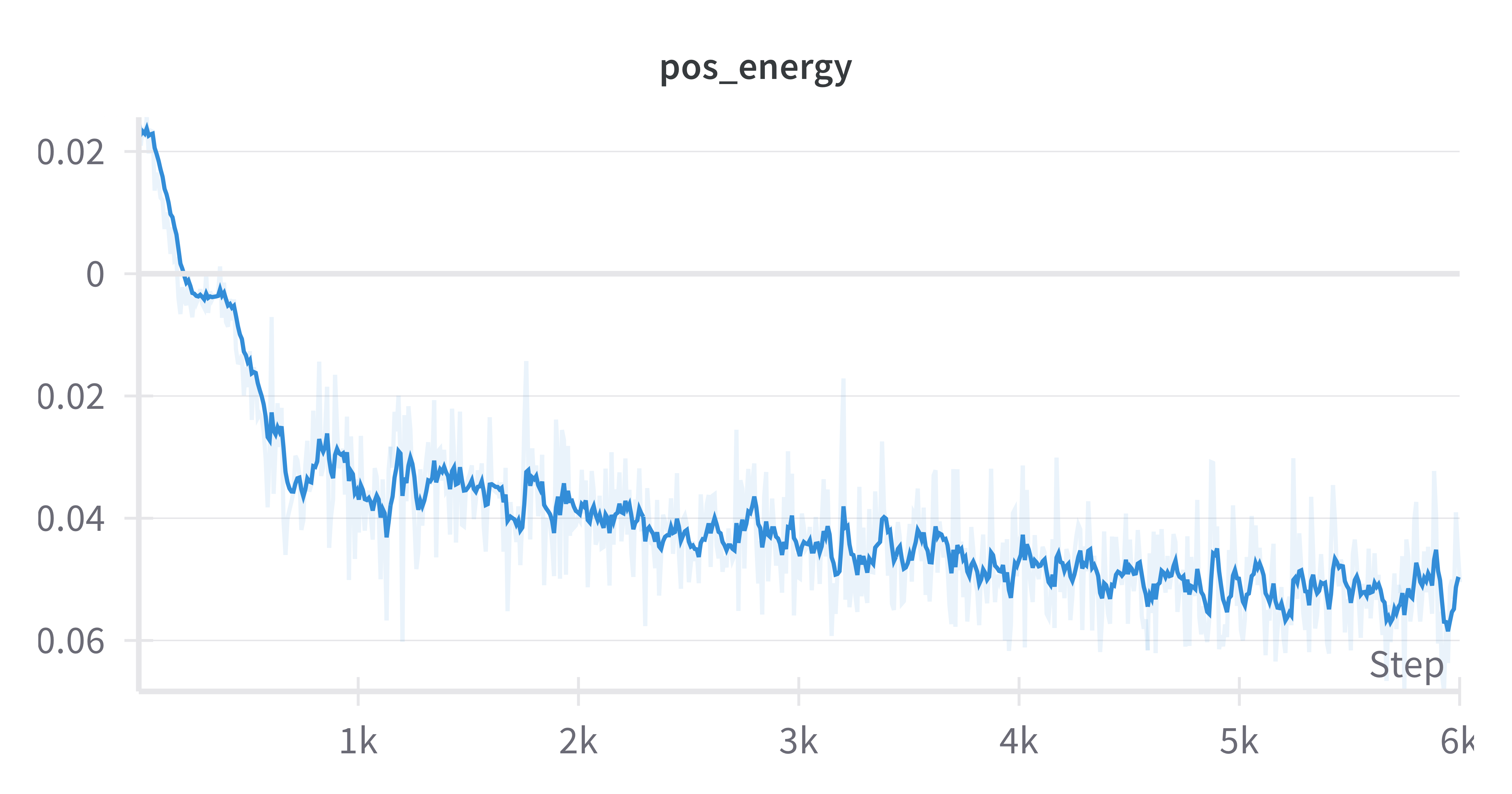
(a) Positive energy

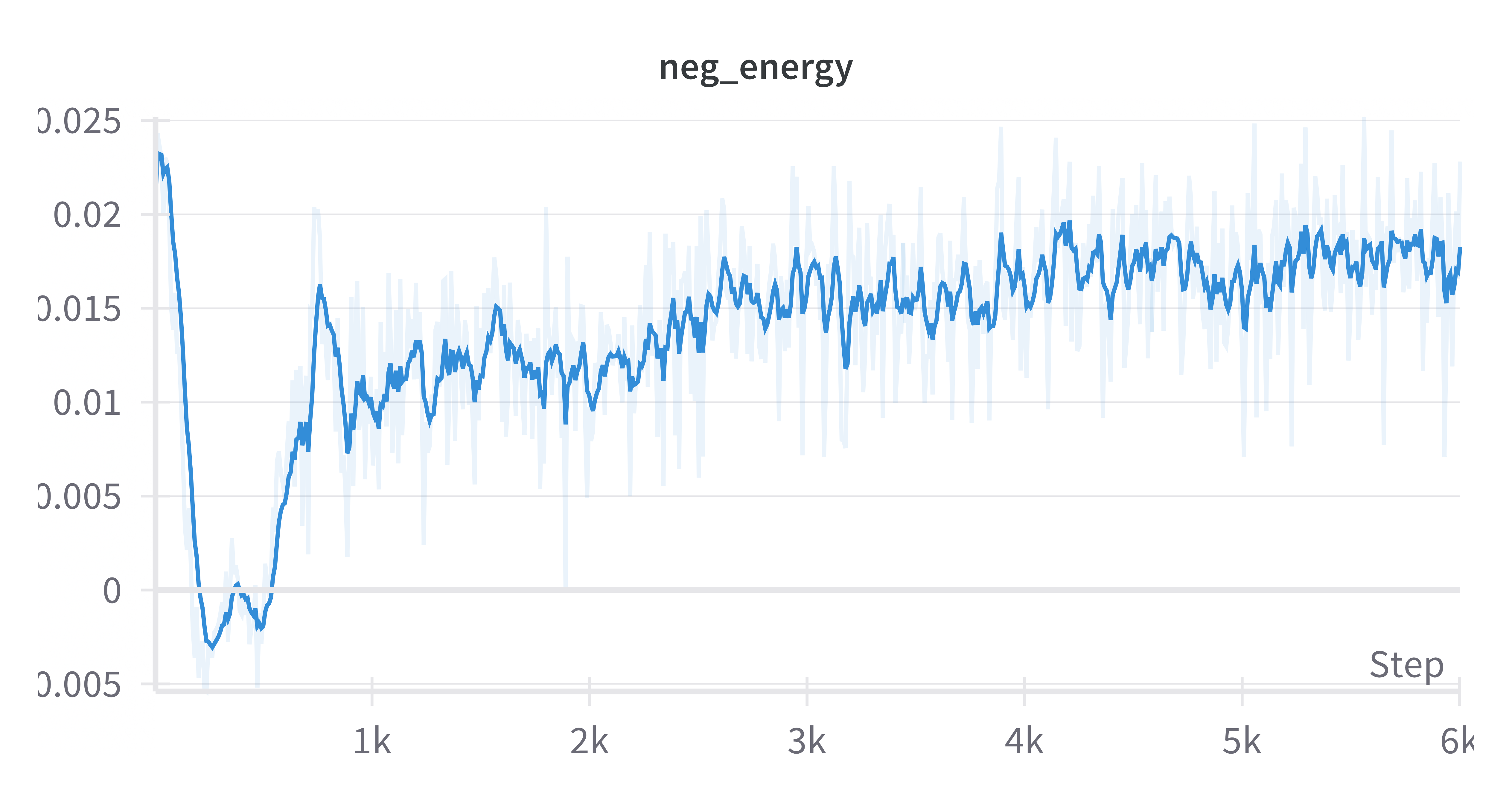
(b) Negative energy

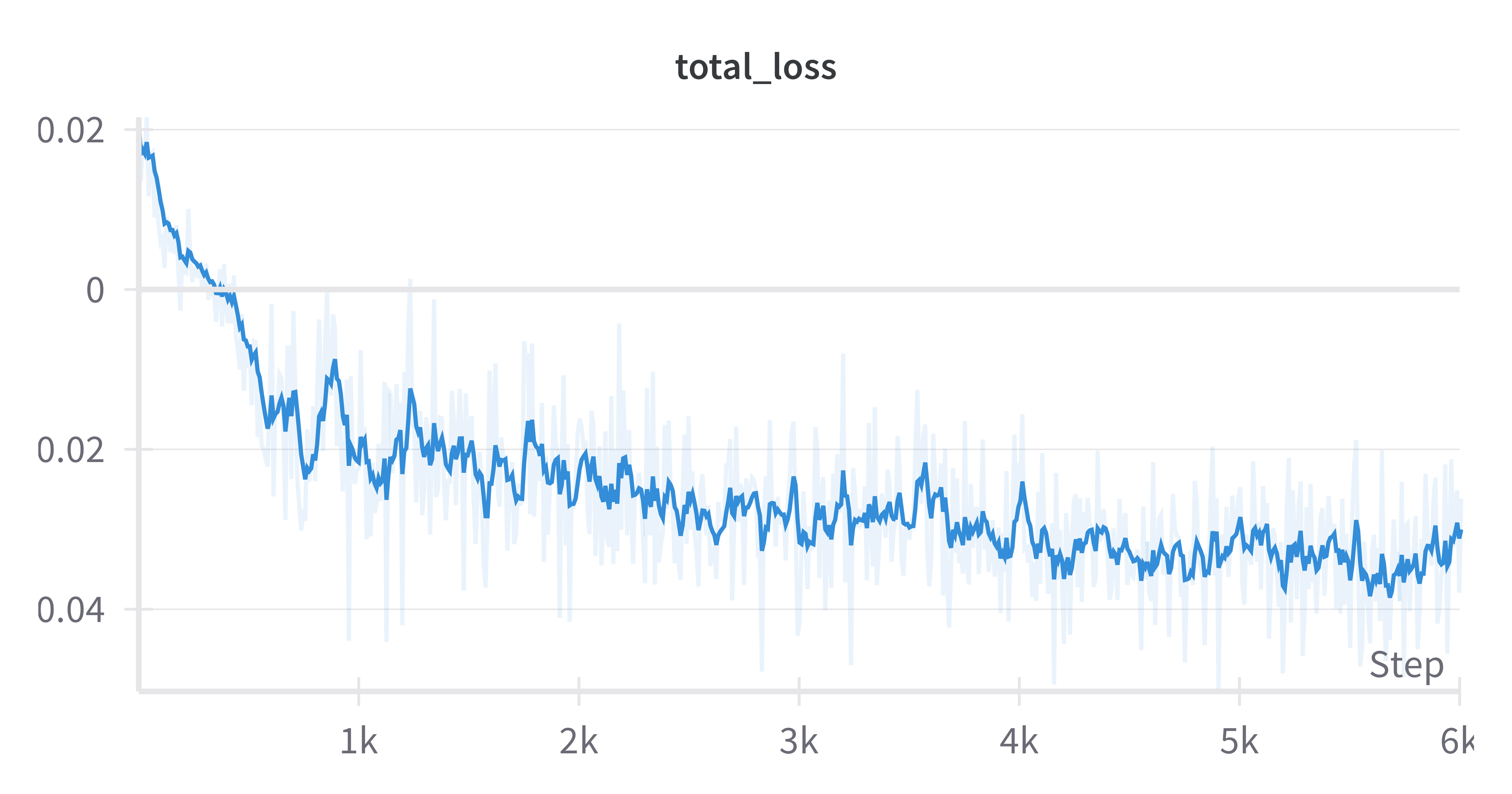
(c) NCE loss

Figure 7: Learning curves for training BBox-Adapter on the StrategyQA dataset.

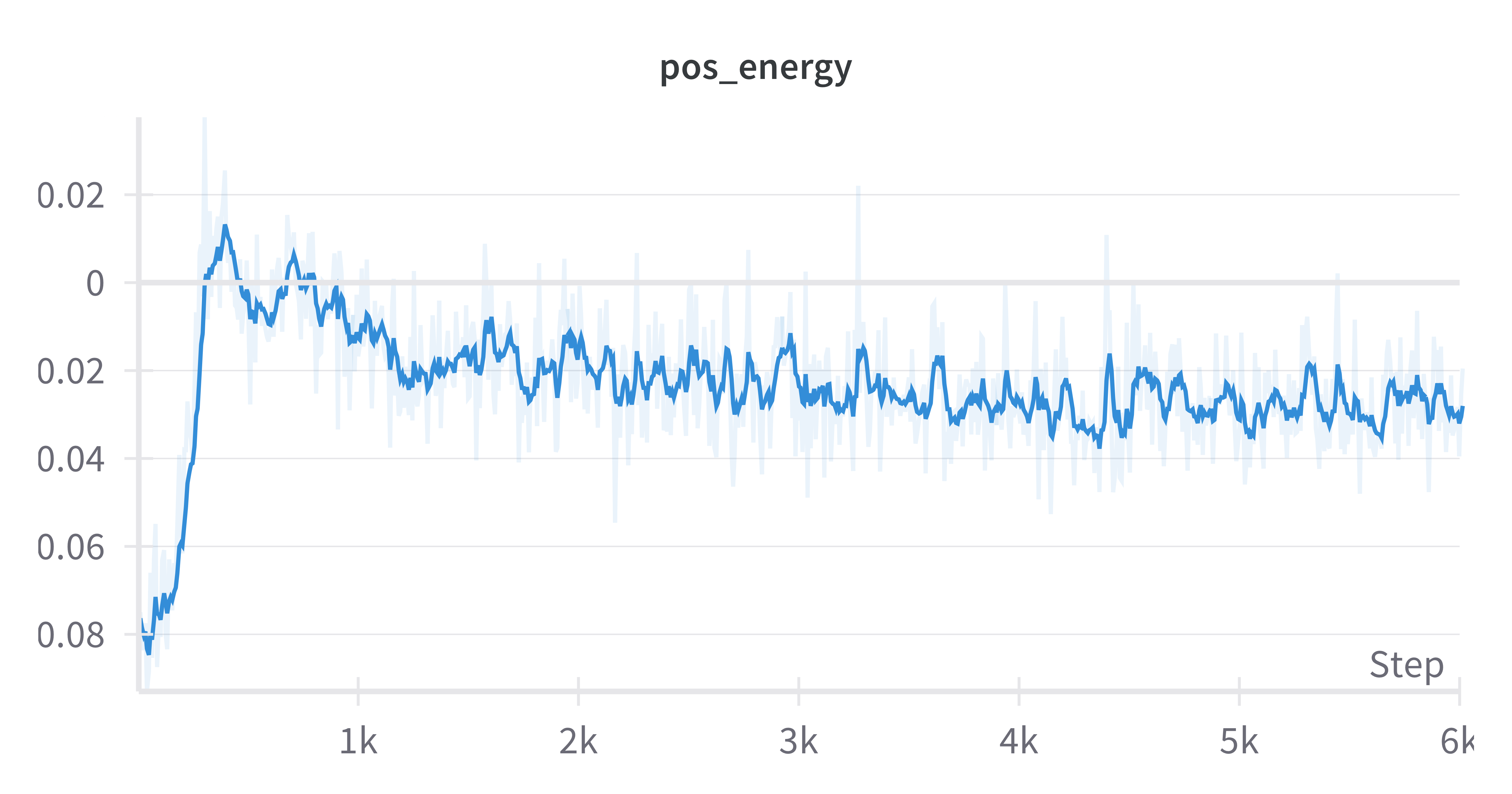
(a) Positive energy

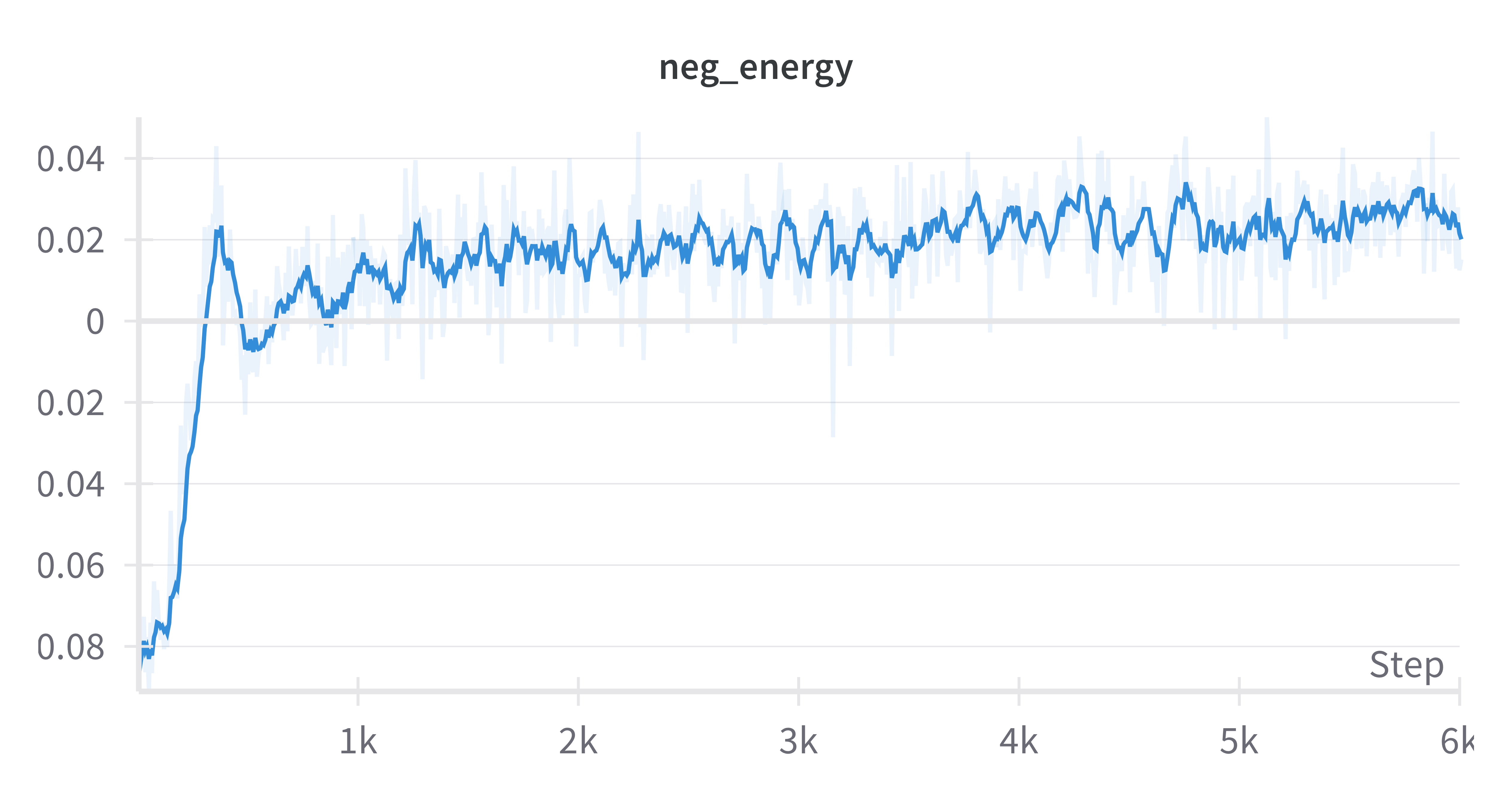
(b) Negative energy

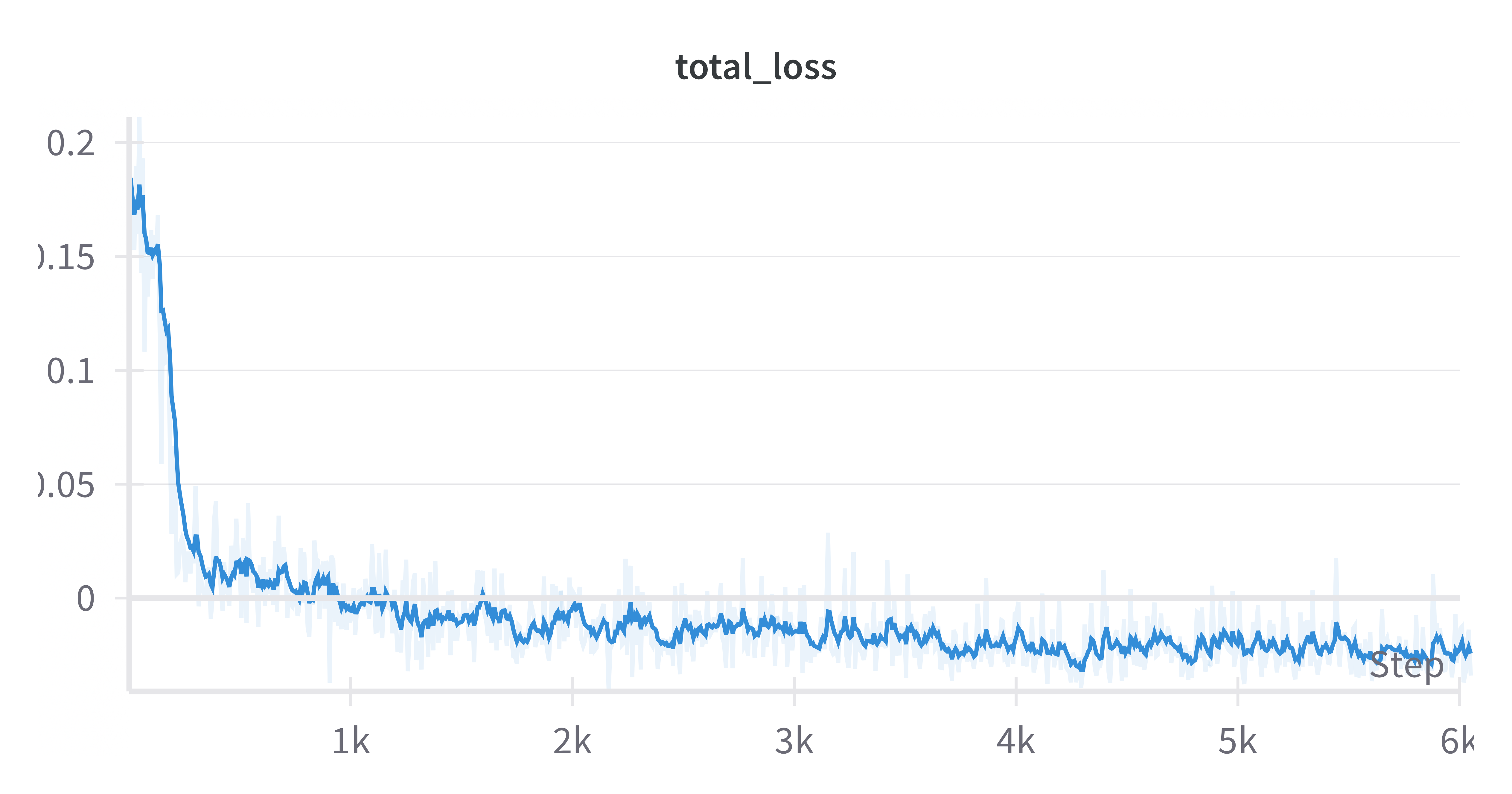
(c) NCE loss

Figure 8: Learning curves for training BBox-Adapter on the GSM8K dataset.

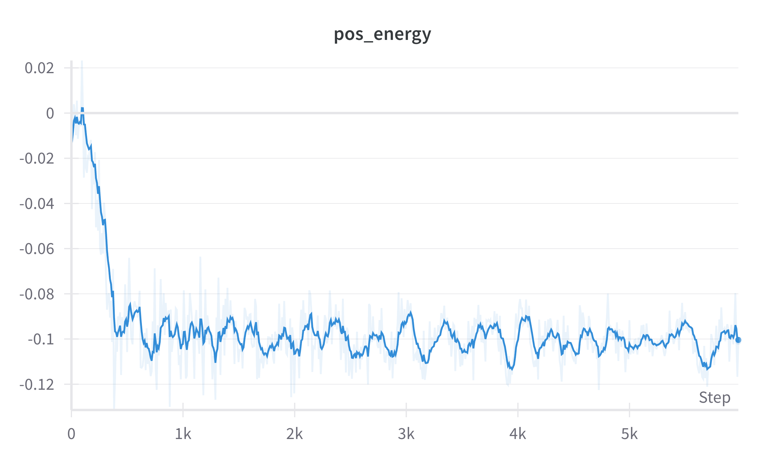
(a) Positive energy

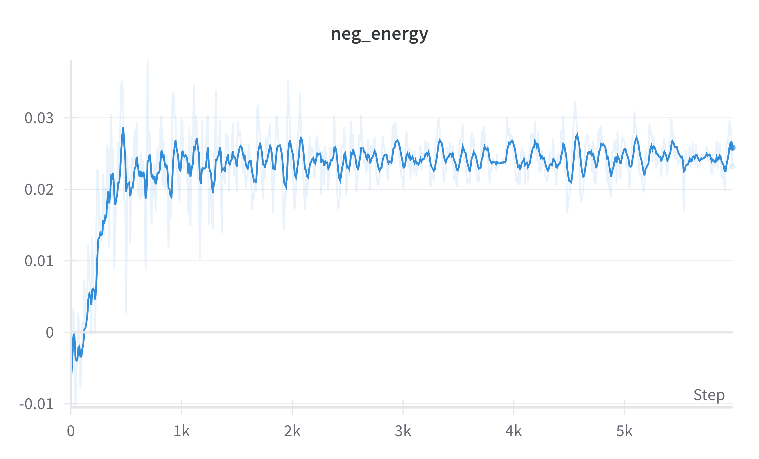
(b) Negative energy

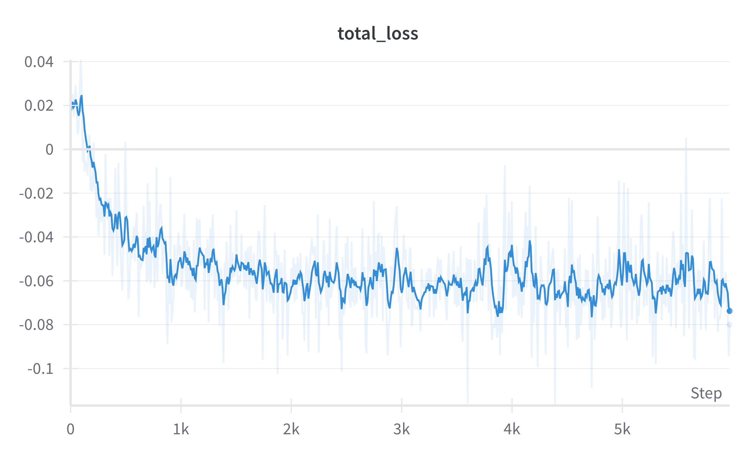
(c) NCE loss

Figure 9: Learning curves for training BBox-Adapter on the TruthfulQA dataset.

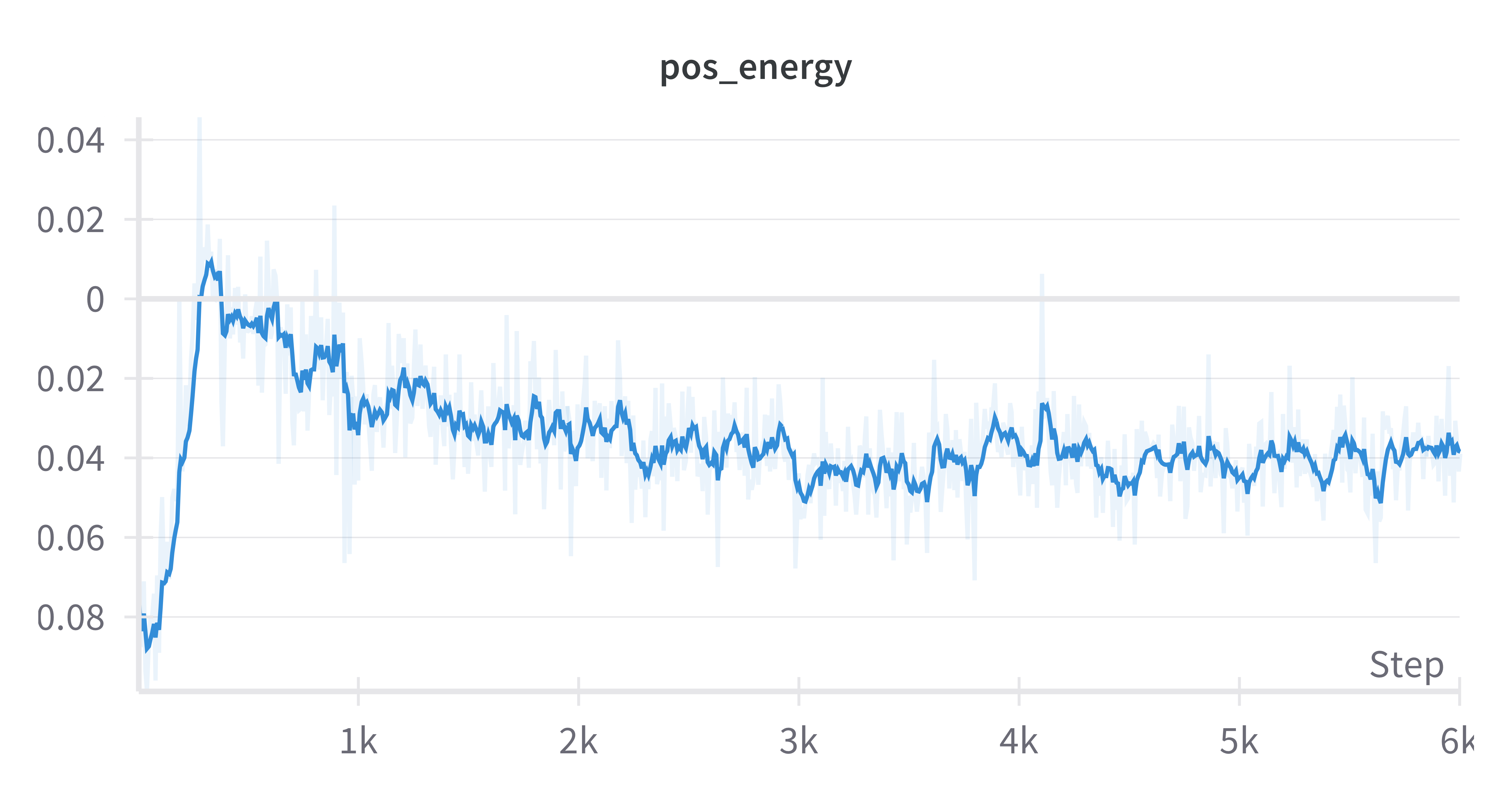
(a) Positive energy

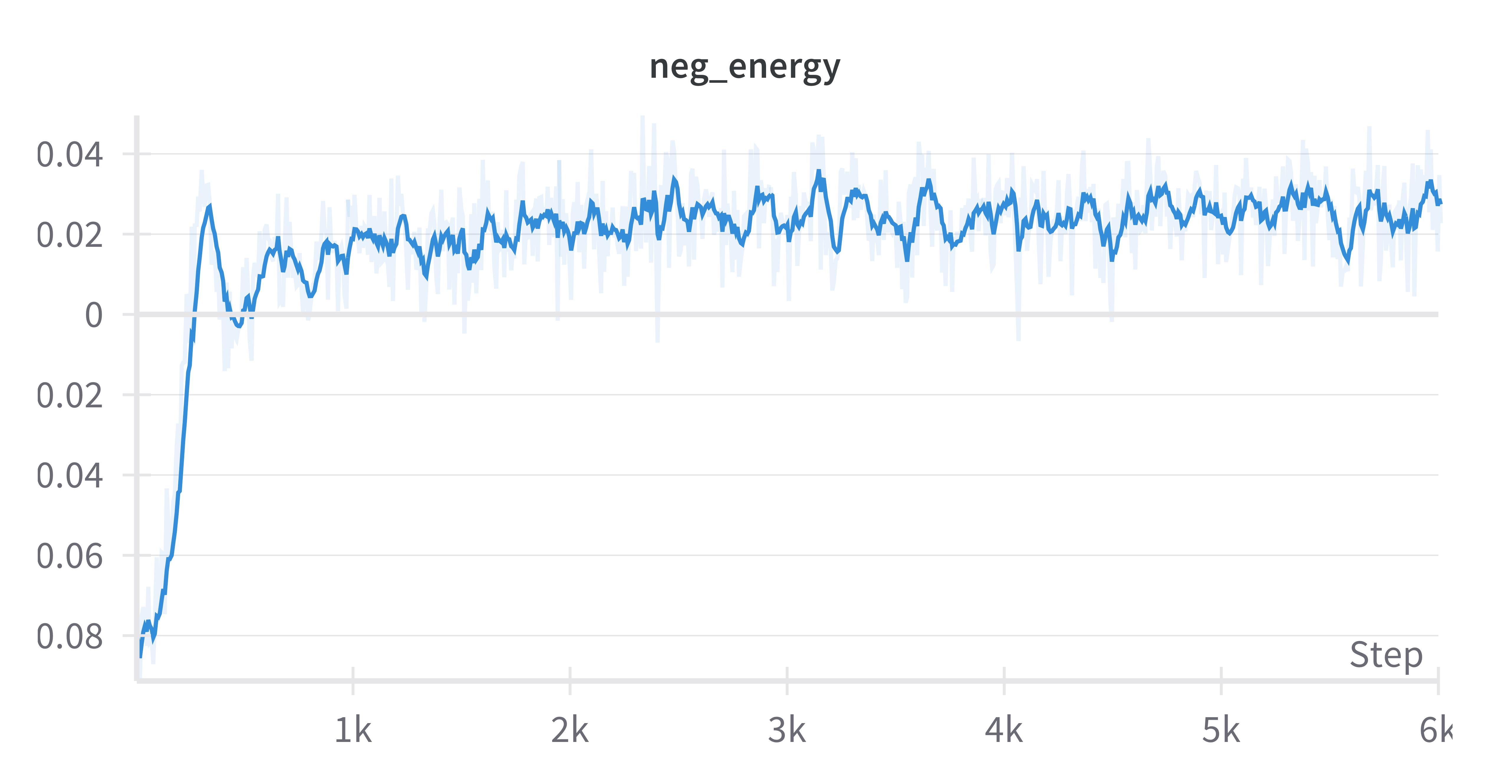
(b) Negative energy

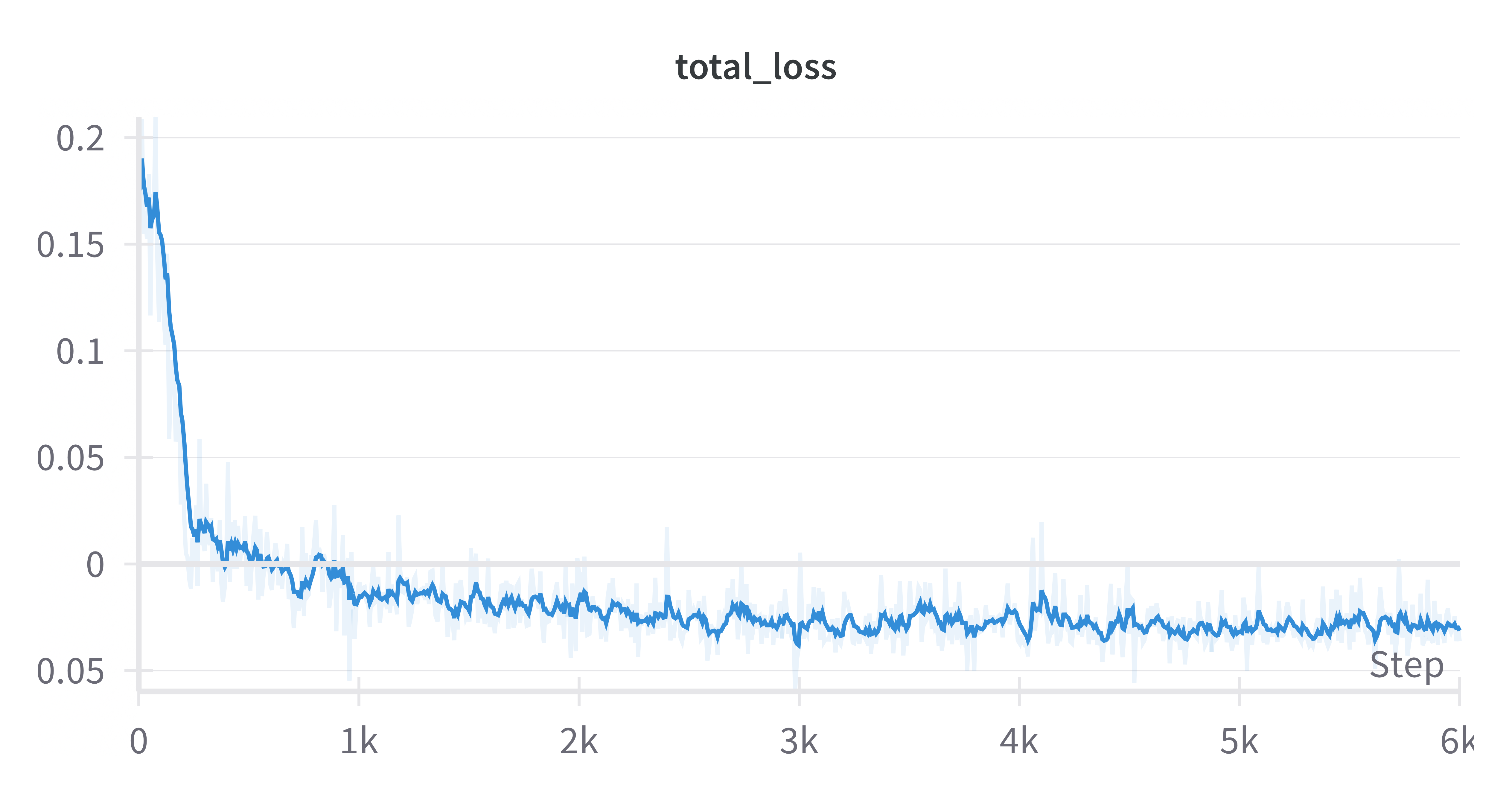
(c) NCE loss

Figure 10: Learning curves for training BBox-Adapter on the ScienceQA dataset.

References

- Anil et al. (2023) Anil, R., Dai, A. M., Firat, O., Johnson, M., Lepikhin, D., Passos, A., Shakeri, S., Taropa, E., Bailey, P., Chen, Z., et al. Palm 2 technical report. arXiv preprint arXiv:2305.10403, 2023.
- Bai et al. (2022) Bai, Y., Kadavath, S., Kundu, S., Askell, A., Kernion, J., Jones, A., Chen, A., Goldie, A., Mirhoseini, A., McKinnon, C., et al. Constitutional ai: Harmlessness from ai feedback. arXiv preprint arXiv:2212.08073, 2022.
- Brown et al. (2020) Brown, T., Mann, B., Ryder, N., Subbiah, M., Kaplan, J. D., Dhariwal, P., Neelakantan, A., Shyam, P., Sastry, G., Askell, A., et al. Language models are few-shot learners. Advances in neural information processing systems, 33:1877–1901, 2020.
- Chowdhery et al. (2022) Chowdhery, A., Narang, S., Devlin, J., Bosma, M., Mishra, G., Roberts, A., Barham, P., Chung, H. W., Sutton, C., Gehrmann, S., et al. Palm: Scaling language modeling with pathways. arXiv preprint arXiv:2204.02311, 2022.
- Chung et al. (2022) Chung, H. W., Hou, L., Longpre, S., Zoph, B., Tay, Y., Fedus, W., Li, Y., Wang, X., Dehghani, M., Brahma, S., et al. Scaling instruction-finetuned language models. arXiv preprint arXiv:2210.11416, 2022.
- Cobbe et al. (2021) Cobbe, K., Kosaraju, V., Bavarian, M., Chen, M., Jun, H., Kaiser, L., Plappert, M., Tworek, J., Hilton, J., Nakano, R., et al. Training verifiers to solve math word problems. arXiv preprint arXiv:2110.14168, 2021.
- Deng et al. (2020) Deng, Y., Bakhtin, A., Ott, M., Szlam, A., and Ranzato, M. Residual energy-based models for text generation. arXiv preprint arXiv:2004.11714, 2020.
- Devlin et al. (2019) Devlin, J., Chang, M.-W., Lee, K., and Toutanova, K. BERT: Pre-training of deep bidirectional transformers for language understanding. In Burstein, J., Doran, C., and Solorio, T. (eds.), Proceedings of the 2019 Conference of the North American Chapter of the Association for Computational Linguistics: Human Language Technologies, Volume 1 (Long and Short Papers), pp. 4171–4186, Minneapolis, Minnesota, June 2019. Association for Computational Linguistics. doi: 10.18653/v1/N19-1423.
- Du & Mordatch (2019) Du, Y. and Mordatch, I. Implicit generation and generalization in energy-based models. arXiv preprint arXiv:1903.08689, 2019.
- Geva et al. (2021) Geva, M., Khashabi, D., Segal, E., Khot, T., Roth, D., and Berant, J. Did aristotle use a laptop? a question answering benchmark with implicit reasoning strategies. Transactions of the Association for Computational Linguistics, 9:346–361, 2021. doi: 10.1162/tacl˙a˙00370.
- Gilardi et al. (2023) Gilardi, F., Alizadeh, M., and Kubli, M. Chatgpt outperforms crowd workers for text-annotation tasks. Proceedings of the National Academy of Sciences, 120(30):e2305016120, 2023. doi: 10.1073/pnas.2305016120.
- Golovneva et al. (2023) Golovneva, O., O’Brien, S., Pasunuru, R., Wang, T., Zettlemoyer, L., Fazel-Zarandi, M., and Celikyilmaz, A. Pathfinder: Guided search over multi-step reasoning paths. arXiv preprint arXiv:2312.05180, 2023.
- Gupta et al. (2023) Gupta, K., Thérien, B., Ibrahim, A., Richter, M. L., Anthony, Q. G., Belilovsky, E., Rish, I., and Lesort, T. Continual pre-training of large language models: How to re-warm your model? In Workshop on Efficient Systems for Foundation Models@ ICML2023, 2023.
- Gururangan et al. (2020) Gururangan, S., Marasović, A., Swayamdipta, S., Lo, K., Beltagy, I., Downey, D., and Smith, N. A. Don’t stop pretraining: Adapt language models to domains and tasks. In Jurafsky, D., Chai, J., Schluter, N., and Tetreault, J. (eds.), Proceedings of the 58th Annual Meeting of the Association for Computational Linguistics, pp. 8342–8360, Online, July 2020. Association for Computational Linguistics. doi: 10.18653/v1/2020.acl-main.740.
- Gutmann & Hyvärinen (2010) Gutmann, M. and Hyvärinen, A. Noise-contrastive estimation: A new estimation principle for unnormalized statistical models. In Proceedings of the thirteenth international conference on artificial intelligence and statistics, pp. 297–304. JMLR Workshop and Conference Proceedings, 2010.
- Hao et al. (2023) Hao, S., Gu, Y., Ma, H., Hong, J., Wang, Z., Wang, D., and Hu, Z. Reasoning with language model is planning with world model. In Bouamor, H., Pino, J., and Bali, K. (eds.), Proceedings of the 2023 Conference on Empirical Methods in Natural Language Processing, pp. 8154–8173, Singapore, December 2023. Association for Computational Linguistics. doi: 10.18653/v1/2023.emnlp-main.507.
- He et al. (2021) He, J., Zhou, C., Ma, X., Berg-Kirkpatrick, T., and Neubig, G. Towards a unified view of parameter-efficient transfer learning. In International Conference on Learning Representations, 2021.
- Houlsby et al. (2019) Houlsby, N., Giurgiu, A., Jastrzebski, S., Morrone, B., De Laroussilhe, Q., Gesmundo, A., Attariyan, M., and Gelly, S. Parameter-efficient transfer learning for nlp. In International Conference on Machine Learning, pp. 2790–2799. PMLR, 2019.
- Hu et al. (2021) Hu, E. J., Wallis, P., Allen-Zhu, Z., Li, Y., Wang, S., Wang, L., Chen, W., et al. Lora: Low-rank adaptation of large language models. In International Conference on Learning Representations, 2021.
- Hu et al. (2023) Hu, N., Mitchell, E., Manning, C., and Finn, C. Meta-learning online adaptation of language models. In Proceedings of the 2023 Conference on Empirical Methods in Natural Language Processing, pp. 4418–4432, Singapore, December 2023. Association for Computational Linguistics.
- Huang et al. (2023) Huang, Y., Liu, D., Zhong, Z., Shi, W., and Lee, Y. T. nn-adapter: Efficient domain adaptation for black-box language models. arXiv preprint arXiv:2302.10879, 2023.
- Jiang et al. (2024) Jiang, A. Q., Sablayrolles, A., Roux, A., Mensch, A., Savary, B., Bamford, C., Chaplot, D. S., Casas, D. d. l., Hanna, E. B., Bressand, F., et al. Mixtral of experts. arXiv preprint arXiv:2401.04088, 2024.
- Kadavath et al. (2022) Kadavath, S., Conerly, T., Askell, A., Henighan, T., Drain, D., Perez, E., Schiefer, N., Hatfield-Dodds, Z., DasSarma, N., Tran-Johnson, E., et al. Language models (mostly) know what they know. arXiv preprint arXiv:2207.05221, 2022.
- Ke et al. (2022) Ke, Z., Shao, Y., Lin, H., Konishi, T., Kim, G., and Liu, B. Continual pre-training of language models. In The Eleventh International Conference on Learning Representations, 2022.
- Khalifa et al. (2023) Khalifa, M., Logeswaran, L., Lee, M., Lee, H., and Wang, L. Grace: Discriminator-guided chain-of-thought reasoning, 2023.
- Lee et al. (2023) Lee, H., Phatale, S., Mansoor, H., Lu, K., Mesnard, T., Bishop, C., Carbune, V., and Rastogi, A. Rlaif: Scaling reinforcement learning from human feedback with ai feedback. arXiv preprint arXiv:2309.00267, 2023.
- Li & Liang (2021) Li, X. L. and Liang, P. Prefix-tuning: Optimizing continuous prompts for generation. In Proceedings of the 59th Annual Meeting of the Association for Computational Linguistics and the 11th International Joint Conference on Natural Language Processing (Volume 1: Long Papers), pp. 4582–4597, 2021.
- Li et al. (2023) Li, Y., Lin, Z., Zhang, S., Fu, Q., Chen, B., Lou, J.-G., and Chen, W. Making language models better reasoners with step-aware verifier. In Rogers, A., Boyd-Graber, J., and Okazaki, N. (eds.), Proceedings of the 61st Annual Meeting of the Association for Computational Linguistics (Volume 1: Long Papers), pp. 5315–5333, Toronto, Canada, July 2023. Association for Computational Linguistics. doi: 10.18653/v1/2023.acl-long.291.
- Lin et al. (2022) Lin, S., Hilton, J., and Evans, O. TruthfulQA: Measuring how models mimic human falsehoods. In Muresan, S., Nakov, P., and Villavicencio, A. (eds.), Proceedings of the 60th Annual Meeting of the Association for Computational Linguistics (Volume 1: Long Papers), pp. 3214–3252, Dublin, Ireland, May 2022. Association for Computational Linguistics. doi: 10.18653/v1/2022.acl-long.229.
- Liu et al. (2024) Liu, A., Han, X., Wang, Y., Tsvetkov, Y., Choi, Y., and Smith, N. A. Tuning language models by proxy, 2024.
- Liu et al. (2022) Liu, X., Ji, K., Fu, Y., Tam, W., Du, Z., Yang, Z., and Tang, J. P-tuning: Prompt tuning can be comparable to fine-tuning across scales and tasks. In Muresan, S., Nakov, P., and Villavicencio, A. (eds.), Proceedings of the 60th Annual Meeting of the Association for Computational Linguistics (Volume 2: Short Papers), pp. 61–68, Dublin, Ireland, May 2022. Association for Computational Linguistics. doi: 10.18653/v1/2022.acl-short.8.
- Lu et al. (2022) Lu, P., Mishra, S., Xia, T., Qiu, L., Chang, K.-W., Zhu, S.-C., Tafjord, O., Clark, P., and Kalyan, A. Learn to explain: Multimodal reasoning via thought chains for science question answering, 2022.
- Ma & Collins (2018) Ma, Z. and Collins, M. Noise contrastive estimation and negative sampling for conditional models: Consistency and statistical efficiency. In Riloff, E., Chiang, D., Hockenmaier, J., and Tsujii, J. (eds.), Proceedings of the 2018 Conference on Empirical Methods in Natural Language Processing, pp. 3698–3707, Brussels, Belgium, October-November 2018. Association for Computational Linguistics. doi: 10.18653/v1/D18-1405.
- Madaan et al. (2023) Madaan, A., Tandon, N., Gupta, P., Hallinan, S., Gao, L., Wiegreffe, S., Alon, U., Dziri, N., Prabhumoye, S., Yang, Y., et al. Self-refine: Iterative refinement with self-feedback. arXiv preprint arXiv:2303.17651, 2023.
- Microsoft (2023) Microsoft. Azure openai gpt 3.5 turbo fine-tuning tutorial. Microsoft Learn Tutorial, 2023.
- Oord et al. (2018) Oord, A. v. d., Li, Y., and Vinyals, O. Representation learning with contrastive predictive coding. arXiv preprint arXiv:1807.03748, 2018.
- OpenAI (2022) OpenAI. Introducing chatgpt. OpenAI Blog, 2022. URL https://openai.com/blog/chatgpt.
- OpenAI (2023) OpenAI. Gpt-4 technical report. arXiv, pp. 2303.08774v3, 2023.
- Ormazabal et al. (2023) Ormazabal, A., Artetxe, M., and Agirre, E. CombLM: Adapting black-box language models through small fine-tuned models. In Bouamor, H., Pino, J., and Bali, K. (eds.), Proceedings of the 2023 Conference on Empirical Methods in Natural Language Processing, pp. 2961–2974, Singapore, December 2023. Association for Computational Linguistics. doi: 10.18653/v1/2023.emnlp-main.180.
- Paul et al. (2023) Paul, D., Ismayilzada, M., Peyrard, M., Borges, B., Bosselut, A., West, R., and Faltings, B. Refiner: Reasoning feedback on intermediate representations. arXiv preprint arXiv:2304.01904, 2023.
- Peng et al. (2023) Peng, A., Wu, M., Allard, J., Kilpatrick, L., and Heidel, S. Gpt-3.5 turbo fine-tuning and api updates. OpenAI Blog, 2023. URL https://openai.com/blog/gpt-3-5-turbo-fine-tuning-and-api-updates.
- Radford et al. (2018) Radford, A., Narasimhan, K., Salimans, T., and Sutskever, I. Improving language understanding by generative pre-training. OpenAI Blog, 2018.
- Radford et al. (2019) Radford, A., Wu, J., Child, R., Luan, D., Amodei, D., and Sutskever, I. Language models are unsupervised multitask learners. OpenAI Blog, 2019.
- Shinn et al. (2023) Shinn, N., Cassano, F., Gopinath, A., Narasimhan, K. R., and Yao, S. Reflexion: Language agents with verbal reinforcement learning. In Thirty-seventh Conference on Neural Information Processing Systems, 2023.
- Sun et al. (2022) Sun, T., Shao, Y., Qian, H., Huang, X., and Qiu, X. Black-box tuning for language-model-as-a-service. In International Conference on Machine Learning, pp. 20841–20855. PMLR, 2022.
- Team et al. (2023) Team, G., Anil, R., Borgeaud, S., Wu, Y., Alayrac, J.-B., Yu, J., Soricut, R., Schalkwyk, J., Dai, A. M., Hauth, A., et al. Gemini: a family of highly capable multimodal models. arXiv preprint arXiv:2312.11805, 2023.
- Touvron et al. (2023) Touvron, H., Martin, L., Stone, K., Albert, P., Almahairi, A., Babaei, Y., Bashlykov, N., Batra, S., Bhargava, P., Bhosale, S., et al. Llama 2: Open foundation and fine-tuned chat models. arXiv preprint arXiv:2307.09288, 2023.
- Wang et al. (2023a) Wang, P., Li, L., Chen, L., Song, F., Lin, B., Cao, Y., Liu, T., and Sui, Z. Making large language models better reasoners with alignment. arXiv preprint arXiv:2309.02144, 2023a.
- Wang et al. (2023b) Wang, P., Li, L., Shao, Z., Xu, R., Dai, D., Li, Y., Chen, D., Wu, Y., and Sui, Z. Math-shepherd: A label-free step-by-step verifier for llms in mathematical reasoning. arXiv preprint arXiv:2312.08935, 2023b.
- Wang et al. (2022a) Wang, X., Wei, J., Schuurmans, D., Le, Q. V., Chi, E. H., Narang, S., Chowdhery, A., and Zhou, D. Self-consistency improves chain of thought reasoning in language models. In The Eleventh International Conference on Learning Representations, 2022a.
- Wang et al. (2022b) Wang, Y., Mishra, S., Alipoormolabashi, P., Kordi, Y., Mirzaei, A., Naik, A., Ashok, A., Dhanasekaran, A. S., Arunkumar, A., Stap, D., Pathak, E., Karamanolakis, G., Lai, H., Purohit, I., Mondal, I., Anderson, J., Kuznia, K., Doshi, K., Pal, K. K., Patel, M., Moradshahi, M., Parmar, M., Purohit, M., Varshney, N., Kaza, P. R., Verma, P., Puri, R. S., Karia, R., Doshi, S., Sampat, S. K., Mishra, S., Reddy A, S., Patro, S., Dixit, T., and Shen, X. Super-NaturalInstructions: Generalization via declarative instructions on 1600+ NLP tasks. In Goldberg, Y., Kozareva, Z., and Zhang, Y. (eds.), Proceedings of the 2022 Conference on Empirical Methods in Natural Language Processing, pp. 5085–5109, Abu Dhabi, United Arab Emirates, December 2022b. Association for Computational Linguistics. doi: 10.18653/v1/2022.emnlp-main.340.
- Wei et al. (2021) Wei, J., Bosma, M., Zhao, V., Guu, K., Yu, A. W., Lester, B., Du, N., Dai, A. M., and Le, Q. V. Finetuned language models are zero-shot learners. In International Conference on Learning Representations, 2021.
- Wei et al. (2022) Wei, J., Wang, X., Schuurmans, D., Bosma, M., Xia, F., Chi, E., Le, Q. V., Zhou, D., et al. Chain-of-thought prompting elicits reasoning in large language models. Advances in Neural Information Processing Systems, 35:24824–24837, 2022.
- Xie et al. (2023) Xie, Y., Kawaguchi, K., Zhao, Y., Zhao, X., Kan, M.-Y., He, J., and Xie, Q. Self-evaluation guided beam search for reasoning. In Thirty-seventh Conference on Neural Information Processing Systems, 2023.
- Yao et al. (2023) Yao, S., Yu, D., Zhao, J., Shafran, I., Griffiths, T. L., Cao, Y., and Narasimhan, K. R. Tree of thoughts: Deliberate problem solving with large language models. In Thirty-seventh Conference on Neural Information Processing Systems, 2023.
- Zhou et al. (2022) Zhou, D., Schärli, N., Hou, L., Wei, J., Scales, N., Wang, X., Schuurmans, D., Cui, C., Bousquet, O., Le, Q. V., et al. Least-to-most prompting enables complex reasoning in large language models. In The Eleventh International Conference on Learning Representations, 2022.
- Zhu et al. (2023) Zhu, X., Wang, J., Zhang, L., Zhang, Y., Huang, Y., Gan, R., Zhang, J., and Yang, Y. Solving math word problems via cooperative reasoning induced language models. In Rogers, A., Boyd-Graber, J., and Okazaki, N. (eds.), Proceedings of the 61st Annual Meeting of the Association for Computational Linguistics (Volume 1: Long Papers), pp. 4471–4485, Toronto, Canada, July 2023. Association for Computational Linguistics. doi: 10.18653/v1/2023.acl-long.245.
- Zhuang et al. (2023) Zhuang, Y., Chen, X., Yu, T., Mitra, S., Bursztyn, V., Rossi, R. A., Sarkhel, S., and Zhang, C. Toolchain*: Efficient action space navigation in large language models with a* search. arXiv preprint arXiv:2310.13227, 2023.