Integrable Approximations of Dispersive Shock Waves of the Granular Chain

Abstract

In the present work we revisit the shock wave dynamics in a granular chain with precompression. By approximating the model by an $\alpha$-Fermi-Pasta-Ulam-Tsingou chain, we leverage the connection of the latter in the strain variable formulation to two separate integrable models, one continuum, namely the KdV equation, and one discrete, namely the Toda lattice. We bring to bear the Whitham modulation theory analysis of such integrable systems and the analytical approximation of their dispersive shock waves in order to provide, through the lens of the reductive connection to the granular crystal, an approximation to the shock wave of the granular problem. A detailed numerical comparison of the original granular chain and its approximate integrable-system based dispersive shocks proves very favorable in a wide parametric range. The gradual deviations between (approximate) theory and numerical computation, as amplitude parameters of the solution increase are quantified and discussed.

I Introduction

Granular chains consist of closely packed arrays of particles that interact elastically upon compression. They have received much recent attention due to their potential in applications (such as shock absorption, frequency conversion, and energy harvesting), recent advances in experimental platforms (including heterogeneous and random ones, ones involving mass-in-mass, mass-with-mass, branching, and intruder-based ones) and the mathematical richness of the underlying equations. See  Nester2001 ; granularBook ; yuli_book ; gc_review ; sen08 for comprehensive reviews on granular chains. From a fundamental perspective, there are three structures of granular chains of central importance: The solitary wave, the breather, and the dispersive shock wave. While the solitary wave and breather have been studied extensively in the context of such nonlinear lattices, its dispersive shock waves (DSWs) are far less understood.

A DSW connects states of different amplitude via an expanding modulated wave train. The study of DSWs in spatially continuous media has been an active area of research since Whitham’s seminal work Whitham74 over 50 years ago. There has been, however, a renewed excitement concerning DSWs. This has largely been inspired by groundbreaking experiments observing DSWs in ultracold gases, optics, superfluids, electron beams, and plasmas dsw ; Hoefer2016 ; Trillo2018 . The new body of mathematical work is summarized in recent review articles on the subject scholar ; Mark2016 ; dsw . Dispersive shock waves in one-dimensional (1D) nonlinear lattices (to be called lattice DSWs) have been explored numerically, and even experimentally in several works first_DSW ; Nester2001 ; Hascoet2000 ; Herbold07 ; Molinari2009 ; shock_trans_granular ; HEC_DSW . Although much of the above motivation stems from the granular chains, it is of broad physical interest, as similar structures have been experimentally observed, e.g., in nonlinear optics of waveguide arrays fleischer2 . It is important to also highlight in this context another setup that has recently emerged, namely tunable magnetic lattices talcohen . Here, ultraslow shock waves can arise and have been experimentally imaged.

The primary tool to analytically describe DSWs is the so-called Whitham modulation theory Whitham74 ; GP73 ; Karpman . In this framework, one derives equations describing slow modulations of the underlying parameters of a periodic wave by, for example, averaging the Lagragian action integral over a family of periodic wave trains dsw ; Mark2016 . The existence of periodic waves has been proved Iooss2000 ; Pankov05 ; Herrmann10b and corresponding modulation equations have been derived Venakides99 ; DHM06 . Explicit forms of the periodic waves may, however, not be available, resulting in modulation equations that are difficult to work with. Thus, in order to get a better understanding of DSWs beyond numerical computations, it is useful to explore additional avenues beyond direct use of the modulation equations. For instance, in marchant2012 analytical techniques to estimate the leading and trailing amplitudes are described. Recently in CHONG2022133533 a discrete conservation law was studied via a reduction to planar ODE dynamics.

In this work, we will revisit the central and experimentally tractable problem of DSW formation in the prototypical setting of granular crystals first_DSW ; Nester2001 ; Hascoet2000 ; Herbold07 ; Molinari2009 ; shock_trans_granular ; HEC_DSW . In the past, and for different structures of this system, such as the traveling waves, resorting to continuum (such as the Korteweg-de Vries (KdV) equation) or discrete (such as the Toda lattice) integrable and hence analytically tractable limits has proven to be of considerable value Shen . It is indeed that route that we will examine herein for the realm of dispersive shock waves. We will explore, in particular, how to exploit existing knowledge on DSWs in those systems to better understand DSWs of the granular chain, but also to explore the extent of the validity of those approximations. Their validity should not be taken for granted, since, e.g., in the case of the KdV equation, the long wavelength assumption needed for its derivation is violated in the case of step initial data in which DSWs arise.

Our presentation will be structured as follows. In section II we will briefly describe the underlying discrete granular problem. Then, in section III, we will delve into the DSW description for the KdV model and its connection/comparison with the granular one. In section IV, we will perform the corresponding analysis and comparison in the case of the Toda lattice. Finally, in section V, we will summarize our findings and present our conclusions and some possible directions for future studies.

II Model Equations for the Granular Chain

An idealized model of the monomer granular chain is given by Nester2001 ; granularBook ; yuli_book ; gc_review ; sen08

$$M\ddot{u}_{n}=\gamma[d_{0}+u_{n-1}-u_{n}]_{+}^{p}-\gamma[d_{0}+u_{n}-u_{n+1}]_{+}^{p},$$ (1)

where $M$ is the effective mass of each node and $u_{n}=u_{n}(t)\in{\mathbb{R}}$ represents the displacement of node $n$ from its equilibrium position at time $t\in{\mathbb{R}}$. In the case of spherical particles the nonlinear exponent is $p=3/2$ (other exponents are also possible depending on the geometry, contact angle, and even material type nesterenko07 ). The parameter $d_{0}$ represents a static displacement (the so-called precompression) that allows additional tunability in the degree of nonlinearity (where $d_{0}=0$ represents a purely nonlinear force and $|d_{0}/x|\gg 1$ represents a nearly linear force). The brackets account for the fact that there is no force in the absence of contact, i.e. $[x]_{+}=\max(0,x)$. While Eq. (1) ignores effects such as dissipation, it has proven to be a reliable model when compared against experiments Nester2001 ; HEC_DSW ; origami2 ; moleron .

In the case of nonzero precompression ($d_{0}\neq 0$), a Taylor approximation of the inter-particle force $\gamma(d_{0}-x)^{p}$ can be used, which, when neglecting all terms beyond cubic powers, reduces the granular chain model to the Fermi-Pasta-Ulam-Tsingou model FPU55 of the form:

$$\ddot{u}_{n}=K_{2}(u_{n-1}-2u_{n}+u_{n+1})+K_{3}\left[(u_{n+1}-u_{n})^{2}-(u_{n}-u_{n-1})^{2}\right]+K_{4}\left[(u_{n+1}-u_{n})^{3}-(u_{n}-u_{n-1})^{3}\right]$$ (2)

where

$$K_{2}=\frac{p\gamma d_{0}^{p-1}}{M},\,K_{3}=-\frac{p(p-1)}{2M}\gamma d_{0}^{p-2},\,K_{4}=\frac{p(p-1)(p-2)}{6M}\gamma d_{0}^{p-3}.$$

This approximation assumes that the strain $y_{n}=u_{n}-u_{n+1}$ is small relative to the precompression, i.e. $|y_{n}|\ll d_{0}$ for all $n$. Thus, oscillations should not exceed the overlap caused by the precompression, suggesting the particles will remain in contact, hence the dropping of the bracket notation. For the graphs in this paper, we will plot the strain $y_{n}$, since the size of $y_{n}$ will tell us how close we are to the assumption $|y_{n}|\ll d_{0}$. With this definition of the strain, waves with $y_{n}>0$ imply the beads are squeezed beyond the precompression amount, and are in this sense compression waves. On the other hand, waves with $y_{n}<0$ imply the beads are squeezed less than the precompression amount. While the beads may still be physically compressed, waves with $y_{n}<0$ can be thought of as a type of tensile wave since they are “stretched” relative to the precompression amount. If $y_{n}<-d_{0}$ then the beads at the lattice sites $n$ and $n+1$ lose contact, and the nonlinearity induced by the bracket $[x]_{+}$ is required. The strongly nonlinear cases of $y_{n}\gg d_{0}$ and $y_{n}<-d_{0}$ will not be covered by the analysis in this paper, which deals with the weakly nonlinear limit. Since the granular chain will necessarily have $K_{3}<0$, we can already expect the appearance of compression type waves. Other types of lattices, such as strain-softening ones RarefactionNester , will have $K_{3}>0$, and will thus generate tensile waves. The analysis in this paper could be applied to other strain-hardening lattices (where the relevant Taylor expansion has $K_{3}<0$), such as magnetic lattices magBreathers , but not strain-softening ones (where the relevant Taylor expansion has $K_{3}>0$). For all simulations we use the parameter values $\gamma=2^{3/2}/3$, $M=1$, and $d_{0}=1/2$. In this case, the Taylor coefficients are $K_{2}=1$ and $K_{3}=-1/2$. The reason for the choice is convenience when comparing the granular lattice to the Toda chain. Before discussing the Toda approximation, we consider the KdV description, which is simpler.

III KdV Description of the Granular Chain

The connection between the FPUT lattice and the KdV equation dates back to the seminal work of Zabusky and Kruskal Zabusky , and is one of the earliest in the study of nonlinear waves. While many aspects of the FPUT lattice have been explored through the KdV lens FPUreview ; VAINCHTEIN2022 (see also Shen in the context of traveling waves in granular crystals), its DSWs have gained less attention. One notable work in this light is Paleari2006 , which explores the connection of metastability and DSWs using the KdV equation. The KdV equation is derived using a small-amplitude and long wavelength assumption. While the small-amplitude aspect will allow us to move from the granular chain model Eq. (1) to the FPUT model of Eq. (2), the long wavelength assumption is more troubling in the context of DSWs. Riemann initial data clearly violate the long wavelength assumption, and so it is not to clear to what extent, if at all, the KdV description of the granular DSWs will be valid. We explore exactly this question in this section. Since we are reporting results in terms of the strain, it is natural to express Eq. (2) in terms of the strain variable $y_{n}=u_{n}-u_{n+1}$,

$$\ddot{y}_{n}=K_{2}(y_{n-1}-y_{n}+y_{n+1})-K_{3}(y_{n-1}^{2}-2y_{n}^{2}+y_{n+1}^{2})$$ (3)

We leave out the cubic (and other higher order) terms since they will not play a role in the analysis. Upon substitution of the ansatz

$$y_{n}=\varepsilon^{2}Y(X,T),\qquad X=\varepsilon(n-\sigma t),\quad{T}=\varepsilon^{3}t$$ (4)

into Eq. (3) and Taylor expanding the $Y(X\pm\varepsilon,T)$ terms, one finds that the terms up to $\mathcal{O}(\varepsilon^{6})$ in the residual will be eliminated if $Y$ satisfies the following KdV equation,

$$\partial_{T}Y+\frac{\sigma}{24}\partial_{X}^{3}Y-\frac{K_{3}}{\sigma}Y\partial_{X}Y=0,$$ (5)

where the sound speed $\sigma$ is defined through $\sigma^{2}=K_{2}$. Note that, since $K_{3}<0$, the solitary waves of the above KdV equation will have $Y>0$, i.e., the solitary waves of the granular chain are compression waves, as expected. See Shen2014 for a detailed discussion of the KdV (and Toda) description of the granular chain solitary waves. Through the scaling $\tau=\sigma T/24$ and $Z=-\frac{24K_{3}}{\sigma^{2}}Y$ we can cast all KdV coefficients to unity,

$$\partial_{\tau}Z+\partial_{X}^{3}Z+Z\partial_{X}Z=0.$$ (6)

Solutions of this KdV equation that are of critical importance for our purposes are the periodic traveling waves,

$$Z(X,\tau)=r_{1}+r_{2}-r_{3}+2(r_{3}-r_{1})\mathrm{dn}^{2}\left(\sqrt{\frac{r_{3}-r_{1}}{6}}(X-V\tau);m\right),\quad V=\frac{r_{1}+r_{2}+r_{3}}{3},\quad m=\frac{r_{2}-r_{1}}{r_{3}-r_{1}}$$ (7)

which are parameterized by $r_{1},r_{2},r_{3}$, and dn is one of the Jacobi elliptic functions with elliptic parameter $0\leq m\leq 1$ NIST2010 . Notice that the limit of these waves as $m\rightarrow 1$ are the solitary waves of the model.

III.1 DSWs of the KdV equation

The DSWs of the KdV equation (6) are well studied, and represent a textbook example of DSWs. In the seminal paper GP73 , the following initial conditions for Eq. (6) were considered in the KdV case:

$$Z(X,0)=\left\{\begin{split}1,\quad&X<0\\ 0,\quad&X>0\end{split}\right.$$ (8)

Assuming the parameters of the periodic wave (e.g., the $r_{j}$) as varying slowly with respect to $X,\tau$ and averaging three of the conserved quantities of the KdV equation over a period yields a set of three Whitham modulation equations Whitham74 . In the case of self-similar solutions, $r_{j}=r_{j}(X/\tau)$, these equations have the form $(S_{j}-X/\tau)r^{\prime}(X/\tau)=0$, where the characteristic speeds $S_{j}$ are nonlinear functions of $r_{1},r_{2}$ and $r_{3}$. Thus, in this self-similar framework, that $r_{j}$ is either constant, or $X/\tau$ is equivalent to the characteristic speed $S_{j}$. Assuming step initial data of the form of Eq. (8) one finds GP73 ,

$$r_{1}=0,\qquad r_{2}=m,\qquad r_{3}=1.$$

Substituting these expressions into Eq. (7), one obtains the following formula for the KdV DSW,

$$Z(X,\tau)=2\mathrm{dn}^{2}\left(\sqrt{\frac{1}{6}}\bigg{(}X-\frac{1+m}{3}\tau\bigg{)};m\right)-(1-m)$$ (9)

where $X,\tau$ are parameterized by $m$ through the expression

$$X/\tau=S(m)\,,$$ (10)

with $S(m)$ the second characteristic velocity of the Whitham equations (where the subscript 2 was ignored for simplicity), namely

$$S(m)=\frac{1+m}{3}-\frac{2}{3}\frac{m(1-m)K(m)}{E(m)-(1-m)K(m)},$$ (11)

and $K(m)$ and $E(m)$ are complete elliptic integrals of the first and second kind, respectively. Details for the derivation of this expression can be found in Gurevich1987 ; Kamchatnov ; Mark2016 . In Eq. (9), the limit $m\rightarrow 0$ corresponds to the trailing, harmonic wave edge, while the limit $m\rightarrow 1$ corresponds to the leading, solitary wave edge. The trailing edge speed ($S_{-}$) and leading edge speed ($S_{+}$) are obtained as limiting values in Eq. (11). In particular

$$\lim_{m\rightarrow 0}S(m)=S_{-}=-1,\qquad\lim_{m\rightarrow 1}S(m)=S_{+}=2/3$$ (12)

Translating back to the granular chain variables, $y_{n}(t)$, we obtain the following approximation for the core of the granular chain DSW:

$$y_{n}(t)=-c\frac{\sigma^{2}}{K_{3}}\left(2\mathrm{dn}^{2}\left(\sqrt{4c}\left(n-\left(1+\frac{m+1}{3}c\right)\sigma t+\theta_{0}(n,t)\right);m\right)-(1-m)\right)$$ (13)

where $c=\varepsilon^{2}/24$ is a small parameter, and the variables $n,t$ are parameterized by $m$ through the expression

$$\frac{(n-\sigma t)}{\sigma ct}=S(m)\,,$$ (14)

with $S(m)$ still given by Eq. (11). Note Eq. (13) contains a slowly modulated phase shift $\theta_{0}(n,t)$ that is not accounted for by the leading order Whitham theory SIAP59p2162 . We have included it here, as it will be treated as a fitting parameter to account for a phase mismatch between theory and simulation.

From the above expression we can write the trailing edge speed ($n/t=s_{-}^{\rm KdV}$) and leading edge speed $(n/t=s_{+}^{\rm KdV})$ in terms of the original granular chain variables,

$$s_{-}^{\rm KdV} = \sigma+\sigma cS_{-}=\sigma\left(1-c\right)$$ (15a)

$$s_{+}^{\rm KdV} = \sigma+\sigma cS_{+}=\sigma\left(1+\frac{2}{3}c\right).$$ (15b)

Thus the leading edge speed is supersonic, as it necessarily features larger than the sound speed $\sigma$, whereas the trailing edge speed is subsonic. Since the parameter $\varepsilon$ is assumed to be small (and hence also so is $c$), the leading edge is traveling just above the sound speed, and the trailing edge is slightly below. Using the parameter values $K_{2}=1$ and $K_{3}=-\frac{1}{2}$, we have the following estimates for the trailing edge speed, and mean $\bar{y}_{-}^{\rm KdV}$ and the leading edge speed and amplitude $(a_{+}^{\rm KdV})$,

$$s_{-}^{\rm KdV}=1-c,\qquad\bar{y}_{-}^{\rm KdV}=2c,\qquad s_{+}^{\rm KdV}=1+\frac{2}{3}c,\qquad a_{+}^{\rm KdV}=4c.$$ (16)

We write the leading and trailing edge characteristics explicitly with this choice of parameters due to their intimate connection with the Toda predictions. This is also why in Eq. (15) and (16) we used the KdV superscript to distinguish between these approximations and the ones using the Toda lattice, described in section IV.

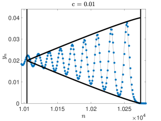
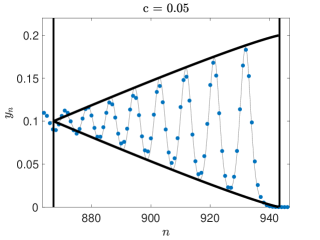
  (a)   (b)   (c)

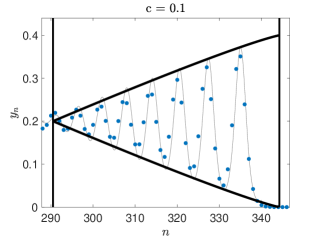
Figure 1: Comparison of the KdV prediction and granular chain simulations in the strain variable, $y_{n}$, for various values of $c$. The KdV predictions, given by Eq. (13), are shown as solid lines, while granular chain simulations with initial data given by Eq. (18), are shown as markers. In all panels, the variables in the KdV scaling are fixed to $T=1200$ and $X\in[-50,30]$. The vertical lines are the predictions of the trailing edge ($n=s_{-}^{\rm KdV}t$) and leading edge ($n=s_{+}t$). The sloped lines are the prediction of the envelopes. (a) The small parameter is $c=0.01$ ($\varepsilon\approx 0.49$) and the time in the original granular chain scaling is $t\approx 10,206$. The best-fit phase shift is the linear interpolation between $\theta_{\ell}=5$ and $\theta_{r}=7$. (b) $c=0.05$ ($\varepsilon\approx 1.1$), $t\approx 912$, $\theta_{\ell}=0$ and $\theta_{r}=1$. (c) $c=0.1$ ($\varepsilon\approx 1.55$), $t\approx 322$, $\theta_{\ell}=-2$ and $\theta_{r}=0.5$.

III.2 Comparison of KdV and granular DSWs

To write down the initial values for the simulation of Eq. (1) that correspond to Eq. (4), we will need the velocity

$$\dot{y}_{n}(t) = \frac{d}{dt}\varepsilon^{2}Y(X,T)$$

$$= -\varepsilon^{3}\sigma\partial_{X}Y+\varepsilon^{5}\left(\frac{K_{3}}{\sigma}Y\partial_{X}Y-\frac{\sigma}{24}\partial_{X}^{3}Y\right)$$

where we used the fact that $Y$ is assumed to solve the KdV equation, Eq. (5). If we substitute $Y(X,0)=-\frac{\sigma^{2}}{24K_{3}}Z(X,0)$ into the above with $Z(X,0)$ defined in Eq. (8), the spatial derivatives will be undefined at $X=0$. Thus, we replace Eq. (8) with a smooth approximation of the unit step, namely,

$$Z(X,0)=\frac{1-\tanh(wX)}{2}=:f(X)$$ (17)

in which case all quantities in the initial value are well-defined. Thus, the initial strain and velocity become,

$$y_{n}(0)=-\frac{\varepsilon^{2}c_{2}^{2}}{24K_{3}}f(\varepsilon n)$$ (18a)

$$\dot{y}_{n}(0)=\frac{\varepsilon^{3}\sigma^{3}}{24K_{3}}f^{\prime}(\varepsilon n)+\frac{\varepsilon^{5}\sigma^{3}}{24^{2}K_{3}}\left(f(\varepsilon n)f^{\prime}(\varepsilon n)+f^{\prime\prime\prime}(\varepsilon n)\right)$$ (18b)

For our first set of simulations, we initialize Eq. (1) with Eqs. (18) with $w=1/2$ and for various values of the parameter $c$, see Fig. 1. In this figure, we select fixed values of the KdV variables $X\in[-50,30]$ and $T_{f}=1200\,(\tau=50)$. For these values of the macroscopic parameters the KdV DSW (see Eq. (9)) is developed, and features about 8 oscillations within its core. To see the DSW in the granular chain develop to the same extent, we must simulate until $t_{f}=\varepsilon^{-3}T_{f}$. Since the leading edge is traveling at the speed $s_{+}$ the lattice must extend at least until $n=s_{+}^{\rm KdV}t_{f}$. For small values of $\varepsilon$ (and hence $c$) this leads to long simulation times with lattices that are quite large, see Fig. 1(a). In this panel, we have $c=0.01$ ($\varepsilon\approx 0.49$), which implies that $t_{f}=10,206$ and that the largest lattice index should exceed $n=10,275$. The maximum strain is approximately $4c=0.04$, which is 8% of the precompression amount $d_{0}=0.5$. This is a fairly weak nonlinear response, and one would hope the KdV approximation to be accurate. Indeed, by comparing the solid lines (KdV approximation) and markers (granular chain simulation) of Fig. 1(a), one sees good agreement. The sloped lines are the prediction of the envelope of the DSW, which is also quite accurate. The vertical lines are the predictions of the trailing edge ($n=s_{-}^{\rm KdV}t$) and leading edge ($n=s_{+}^{\rm KdV}t$). In the figure, one can see linear waves at the trailing edge that do no vanish, while the KdV prediction has vanishing oscillations at the trailing edge. The existence of linear waves at the trailing edge is well known in FPUT lattices. While these linear waves will always be present, their amplitude decays like $\sim t^{-1/3}$ MielkePatz2017 (and they are not expected to be captured through Whitham theory). The leading edge of the actual DSW is lagging behind the predicted location (given by $s_{+}^{\rm KdV}t$). This discprency becomes larger as $c$ is increased (compare panels (a)-(c)). In general, there will be a phase mismatch between the theoretical prediction and the actual granular DSW. To account for this, a phase shift $\theta_{0}(n)$ is applied to the theoretical prediction by finding the best-fit phase shift at the trailing edge of the DSW (to obtain a phase shift $\theta_{\ell}$) and at the leading edge (to obtain a phase shift $\theta_{r}$). Then $\theta_{0}(n)$ is defined as the linear interpolation between these two shifts, namely $\theta_{0}(n)=\frac{\theta_{\ell}-\theta_{r}}{n_{\ell}-n_{r}}(n-n_{r})+\theta_{r}$ where $n_{\ell}$ and $n_{r}$ are lattice indices close to the trailing and leading edge, respectively. We practically used $n_{\ell}=s_{-}^{\rm KdV}t_{f}+5$ and $n_{r}=s_{+}^{\rm KdV}t_{f}-5$. Accounting for the phase in this way results in good agreement between the KdV prediction and actual full profile of the DSW. Note, for reference purposes, that we do not shift the trailing and leading edge, nor the envelope predictions (thus the solid black lines are the “original” prediction without an empirically determined phase shift). There is a number of causes for the phase mismatch between theory and actual DSW. The first is that the initial condition does not lead to the immediate formation of a DSW, since the smooth monotone decreasing initial data first needs to develop a gradient catastrophe. Thus, one would expect the leading solitary wave to lag behind the prediction, due to the later “start” in the simulation. The catastrophe time in the derived KdV equation can be approximated by computing when two arbitrary characteristics lines of the underlying Hopf equation $Z_{\tau}+ZZ_{X}$ intersect, leading to the prediction $\tau_{\rm catastrophe}=-1/\min_{\mathbb{R}}f^{\prime}(X)$ where $f(X)$ is the initial datum defined in Eq. (17). This could be used as a concrete correction for the phase shift. However, it is less obvious how to correct for the other two sources of the phase mismatch. One is the missing phase description from the first order Whitham theory. While such a prediction is possible in principle, the underlying complexity of the correction would undermine the elegant simplicity of the approximation given in Eq. (13). Finally, another source of mismatch will be in the inherent approximate nature of Eq. (4). While bounds for the error of the KdV approximation exist (assuming smoothness of the underlying KdV solutions pegogf1 ; SW00 ), they cannot be used to correct the phase mismatch. Thus, we capture all the possible sources of error in the phase by empirically determining the phase $\theta_{0}(n)$. Even without this empirical correction, the leading and trailing edge, and the envelopes, are well described by the KdV equation. Panels (b) and (c) of Fig. 1 are similar to panel (a), but consider larger values of the parameter $c$, in order to test the practical limits of the approximation. In panel (b) we have $c=0.05$ ($\varepsilon\approx 1.1$), which leads to a maximum strain of about $4c=0.2$, which is 40% of the initial precompression. This is a fairly nonlinear response, and indeed, the parameter $\varepsilon\approx 1.1$ actually exceeds unity, which is in clear violation of the smallness assumption. Nonetheless, the KdV approximation is still quite reasonable. In panel (c) we have $c=0.10$ ($\varepsilon\approx 1.55$), which leads to a maximum strain of about $4c=0.4$, which is 80% of the initial precompression. For such large values of the strain, one can start to see discrepancies between the KdV prediction and granular chain dynamics, even after accounting for the phase mismatch. From a qualitative perspective, however, the agreement remains reasonable considering how large the strain is.

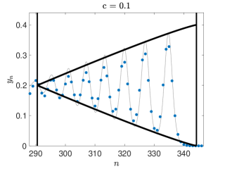
  (a)   (b)   (c)

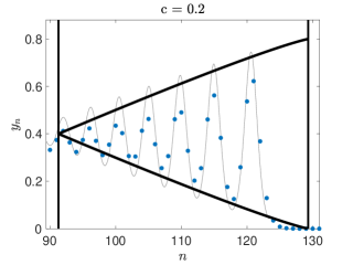
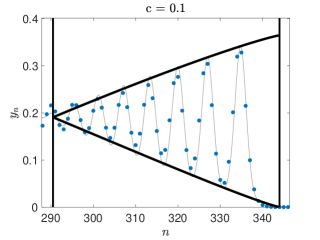
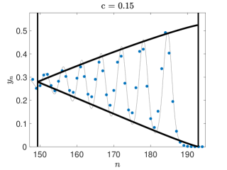
  (d)   (e)   (f)

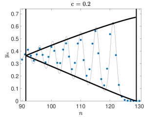
Figure 2: Granular chain simulations with an initial velocity shock, Eq. (19), compared to the KdV prediction (top row) and Toda prediction (bottom row). Theoretical predictions are shown as solid lines and granular chain simulations are shown as markers. In all panels, the variables in the KdV scaling are fixed to $T=1200$ and $X\in[-50,30]$. The vertical lines are the predictions of the trailing and leading edge. The sloped lines are the prediction of the envelopes. (a) The small parameter is $c=0.1$ ($\varepsilon\approx 1.55$) and the time in the original granular chain scaling is $t\approx 322$. The best-fit phase shift is the linear interpolation between $\theta_{\ell}=-4.5$ and $\theta_{r}=0.5$. (b) $c=0.15$ ($\varepsilon\approx 1.9$), $t\approx 175$, $\theta_{\ell}=-5.5$ and $\theta_{r}=-0.5$. (c) $c=0.2$ ($\varepsilon\approx 2.2$), $t\approx 115$, $\theta_{\ell}=-6$ and $\theta_{r}=-1.5$. (d) $c=0.1$ ($\varepsilon\approx 1.55$), $\theta_{\ell}=-3$ and $\theta_{r}=0.2$. (e) $c=0.15$ ($\varepsilon\approx 1.9$), $t\approx 175$, $\theta_{\ell}=-4$ and $\theta_{r}=-0.5$. (f) $c=0.2$ ($\varepsilon\approx 2.2$), $t\approx 115$, $\theta_{\ell}=-4.5$ and $\theta_{r}=-1$.

Figure 1 demonstrates that the KdV approximation of the granular chain DSW is quite good, as long as the parameter $c$ is small. Thinking of the relevance of the description for an experimental setting, a smaller lattice size would be more practically accessible, and thus the speed $c$ should be larger, such that the DSW can form before the end of the chain is reached. Thus, we will next explore going beyond the smallness assumption of $c$ in hopes of getting to lattices of reasonable size (some experiments have chains on the order of 100 beads Boechler2010 and, indeed, khatriprl reports experiments with up to 188 beads). Furthermore, the initial conditions used for Fig. 1 imply the entire strain and velocity profile must be specified, which is generally hard to achieve in granular chain experiments. The more relevant initial condition for the granular chain, and other similar lattices, is a collision at one side of the chain. In Molinari2009 it was shown that such a collision is well approximated by a continuous velocity applied to the end of a semi-infinite chain (this is the so-called piston problem piston ). By an appropriate change of variables, the piston-problem initial conditions are equivalent to an infinite chain with a velocity shock Venakides99 , namely,

$$u_{n}(0)=0$$ (19a)

$$\dot{u}_{n}(0)=-2c\,{\mathrm{sign}}(n)$$ (19b)

where ${\mathrm{sign}}(0)=0$. Notice that this initial condition is given in terms of the displacement variable $u_{n}$. Nonetheless, we continue to report results in terms of the strain $y_{n}=u_{n}-u_{n+1}$ for consistency. With such an initial condition, it is reasonable to suppose, based on the linear theory MielkePatz2017 , that the trailing edge (in the strain) will have a mean close to $2c$.This suggests that the $c$ defined assuming the initial data Eq. (8) is the same as the $c$ defined in Eq. (19). Indeed, this was the motivation for defining $c=\varepsilon^{2}/24$ previously. This means we can apply the prediction Eq. (13), even when the initial condition is given by a velocity shock. The top row of Fig. 2 shows a comparison of a DSW formed given a velocity shock (markers) and the KdV prediction for various values of $c$. Once again, the microscopic time $t$ is chosen such that macroscopic time $T_{f}=1200$ is fixed. This implies that Fig. 1(c) and Fig. 2(a) show the same KdV approximation, but the former granular chain data comes from a smooth shock in the strain, while the latter has a (displacement) velocity shock. By comparing those two figure panels, one can see that the overall structure of the two DSWs is qualitatively similar. Figure 2(b,c) show examples for larger values of $c$, and the discrepancies are becoming more evident. Nonetheless the qualitative agreement is still reasonable. Notice that for $c=0.2$, which corresponds to Figure 2(c), a chain extending to $n=130$ will capture the DSW, which is within the realm of current experimental capabilities, as per our discussion of khatriprl above. The top row of Fig. 3 shows the same simulation data, but now with windowing such that the microscopic variables ($n,t$) are fixed. In particular, intensity plots of the strain are shown. The prediction of the leading and trailing speed from the KdV equation are shown as solid black lines.

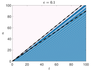
  (a)   (b)   (c)

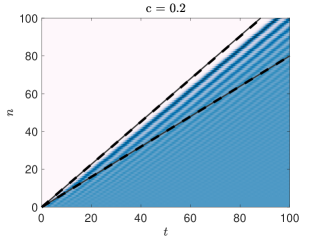
Figure 3: Intensity plots of the granular chain simulations with an initial velocity shock, Eq. (19). The solid lines are the estimates of the leading and trailing edge from the KdV description, and the dashed lines are from the Toda description. (a) $c=0.1$, (b) $c=0.15$ (c) $c=0.2$.

We now investigate how well the estimates of the trailing and leading edge characteristics in Eq. (16) compare to the granular DSWs for a larger range of the parameter $c$. Figure 4(a) shows a numerical estimate of the leading edge amplitude (blue dots). The amplitude is simply the maximum strain observed at the final time of the simulation, which we fixed to $t_{f}=900$ for all simulations shown in the figure. The KdV approximation of the leading edge amplitude, $a_{+}^{\rm KdV}$, is shown as the blue solid line. As expected, the agreement is good for small $c$, but gradually gets worse as $c$ increases. The trailing edge mean of the simulated DSW is shown as the red squares in Figure4(a). It is estimated as the mean of the first node, namely $\frac{1}{T}\int_{I_{T}}y_{1}(t)dt$ where $T$ is the peak to peak time of the final oscillation in the simulation and $I_{T}$ is the corresponding interval of time. The KdV approximation, $\bar{y}_{-}^{\rm KdV}$, is shown as the solid red line. The leading edge (blue dots) and trailing edge (red squares) speeds are shown in Fig. 4(b). The leading speed is estimated by computing the difference in the times the maximum is obtained between two consecutive sites and simply inverting that time difference to obtain the speed estimate. We used the sites $n=700$ and $n=701$. To estimate the trailing edge speed, we select a small amplitude threshold and define the trailing edge to be the first node that achieves a strain higher than or equal to the threshold after having fixed the time to $t=t_{f}$. The estimate for the speed is then simply this critical lattice site divided by $t_{f}$. One must define such a threshold since there will always be the presence of small amplitude linear waves at the trailing edge of the DSW. The threshold we used was the mean of the tail (just described) plus 2.5% of the maximum strain of the DSW. This particular choice of threshold yields good agreement when numerically comparing the trailing speed of the Toda lattice DSW to the analytical prediction (detailed in the next section). The KdV prediction of the edge speeds are shown as the solid lines for the trailing edge, $s_{-}^{\rm KdV}$ (red), and leading edge, $s_{+}^{\rm KdV}$ (blue). From Fig. 4 we see that the KdV prediction overestimates the leading edge amplitude and trailing edge mean, and overestimates (by quite a large margin for large $c$) the DSW core length, given by $(s_{+}^{\rm KdV}-s_{-}^{\rm KdV})t$.

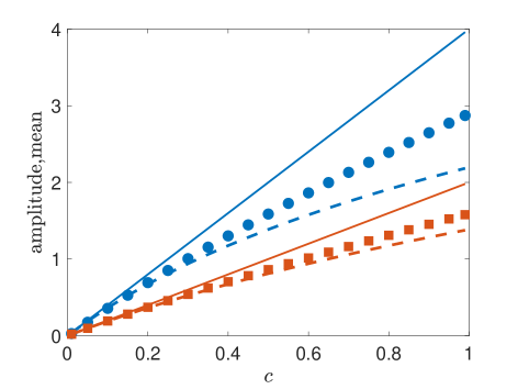
  (a)   (b)

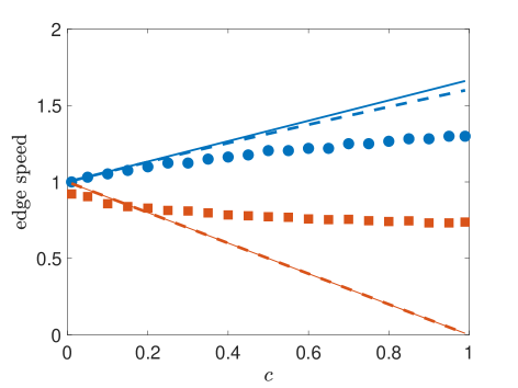
Figure 4: (a) Numerical estimates of the leading edge amplitude (blue dots) and trailing edge mean (red squares) of the granular DSW versus the initial velocity parameter $c$. The corresponding KdV approximation (solid lines) and Toda approximation (dashed lines) are also shown. (b) Numerical estimates of the leading edge speed (blue dots) and trailing edge speed (red squares) of the granular DSW versus the initial velocity parameter $c$. The corresponding KdV approximation (solid lines) and Toda approximation (dashed lines) are also shown.

IV Toda Description of the Granular Chain

We now turn our attention to a different analytical approximation of the granular chain DSW. The latter will be based on the Toda lattice, which is one of the few nonlinear lattices that is integrable (another example is the Kac-van Moerbeke lattice, which is closely related to Toda via a Miura type transformation Moser ). The Toda lattice has a rich history Toda . The equation in its canonical form is

$$\ddot{u}_{n}=e^{u_{n-1}-u_{n}}-e^{u_{n}-u_{n+1}}\,.$$ (20)

If one Taylor expands the relevant ODEs, the following FPUT lattice is obtained,

$$\ddot{u}_{n}=(u_{n-1}-2u_{n}+u_{n+1})-\frac{1}{2}\left[(u_{n+1}-u_{n-1})^{2}-(u_{n}-u_{n-1})^{2}\right]+\frac{1}{6}\left[(u_{n+1}-u_{n-1})^{3}-(u_{n}-u_{n-1})^{3}\right]$$ (21)

Through the rescaling $u_{n}(t)\rightarrow K_{2}/K_{3}u_{n}(t\sqrt{K_{2}})$, we can match the linear and quadratic terms of the Taylor-expanded granular chain (see Eq. (2)) and the Taylor-expanded Toda chain (see Eq. (21)) for an arbitrary choice of the granular chain parameters $d_{0},\gamma,M$ (recall $p=3/2$). Since we can only rescale time and amplitude, we cannot match the cubic coefficients. Notice that a similar matching was leveraged in the work of Shen in order to study traveling waves in granular chains: indeed, in that connection the Toda lattice could afford the possibility of bi-directional waves and their collisions, a feature that is absent from the (unidirectional) KdV approximation. Recall that for convenience we selected $\gamma=2^{3/2}/3$, $M=1$, $d_{0}=1/2$ for the numerical computations, which led to Taylor coefficients $K_{2}=1$ and $K_{3}=-1/2$, which match the first two Toda Taylor coefficients. This was the reason for the choice of parameters used in the previous section, so that we may better compare the KdV and Toda predictions. Recall that the sound speed is $\sigma=1$.

There is a four parameter family of traveling periodic waves of the Toda lattice, parameterized by $E_{1},E_{2},E_{3},E_{4}$. In terms of the strain, the formula is,

$$y_{n}(t)=\log\left(2\hat{R}_{n}(t)+\frac{1}{2}(E_{1}^{2}+E_{2}^{2}+E_{3}^{2}+E_{4}^{2})-\mu_{n}^{2}(t)-b_{n}^{2}(t)\right)$$ (22)

where

$$b_{n}(t)=E_{1}+E_{2}+E_{3}+E_{4}-2\mu_{n}(t)$$ (23)

and

$$\mu_{n}(t)=E_{2}\frac{\displaystyle 1-(E_{1}/E_{2})\,B\,\mathop{\rm sn}\nolimits^{2}(Z_{n}(t),m)}{1-B\,\mathop{\rm sn}\nolimits^{2}(Z_{n}(t),m)}\,,$$ (24a)

$$Z_{n}(t)=2nF(\Delta,m)+\omega t\ +Z_{0},$$ (24b)

$$m=\frac{(E_{3}-E_{2})(E_{4}-E_{1})}{(E_{4}-E_{2})(E_{3}-E_{1})}\,,$$ (24c)

$$\hat{R}_{n}(t)=-\sigma_{n}(t)\,\sqrt{P(\mu_{n}(t))}\,,\qquad P(z)=(z-E_{1})(z-E_{2})(z-E_{3})(z-E_{4})\,,$$ (24d)

$$\omega=\sqrt{(E_{4}-E_{2})(E_{3}-E_{1})}\,,\qquad\Delta=\sqrt{\frac{E_{4}-E_{2}}{E_{4}-E_{1}}}\,,\qquad B=\frac{E_{3}-E_{2}}{E_{3}-E_{1}}\,.$$ (24e)

In the above equations, $\mathop{\rm sn}\nolimits(z,m)$ is the Jacobi elliptic sine, $F(z,m)$ is the inverse of $\mathop{\rm sn}\nolimits(z,m)$, $Z_{0}$ is an arbitrary translation parameter (phase), $\mu_{n}(t)$ is the Dirichlet eigenvalue of the scattering problem for the Toda lattice and $\sigma_{n}(t)=\pm 1$ is the sign associated with $\mu_{n}(t)$, and determines whether $\mu_{n}(t)$ is increasing or decreasing as a function of $n$ and $t$. For numerical computations, we used $\sigma_{n}(t)=-{\mathrm{sign}}(\mod(Z_{n}(t)/K_{m})-1/2)$. Notice how the Toda traveling wave solution is more complicated than its KdV counterpart in Eq. (7). So while we may anticipate a better approximation (since no long-wavelength assumption is made), the cost is a formula that will be more cumbersome.

IV.1 DSWs of the Toda lattice

The Toda shock problem PRB1981v24p2595 ; VDO is the IVP for Eq. (20) with an initial velocity shock, see Eq. (19). Both the shock problem and the rarefaction problem were studied in blochkodama within the framework of Whitham modulation theory. Like in the KdV case, one can derive a system of modulation equations (4 in the Toda case) that can be written in diagonalized form, and solved in the self-similar frame $E_{j}=E_{j}(n/t)$ assuming an initial velocity shock. Three of the parameters are constant in the self-similar frame, and one depends on the parameter $m$ blochkodama ; Gino2023 . In particular,

$$E_{1}=-(1+c),\quad E_{2}=-(c-1),\quad E_{3}(m)=(c+1)\frac{1-c(1-m)}{1+c(1-m)},\quad E_{4}=(c+1).$$ (25)

Assuming $0<c<1$, the core of the DSW is described by Eq. (22) with parameters given via Eq. (25) where $n,t$ are parameterized by $m$ through the expression

$$\frac{c(c+1)}{1+c(1-m)}\frac{(1+c(1-m))E(m)-(c+1)(1-m)K(m)}{(c+1)K(m)-(1+c(1-m))\Pi\left(\left.\frac{cm}{c+1}\right|m\right)}=:s^{\rm Toda}(m)=\frac{n}{t}$$ (26)

where $K(m)$, $E(m)$ and $\Pi(n|m)$ are complete elliptic integrals of the first, second, and third kind respectively, and $s^{\rm Toda}(m)$ is the third charecteristic velocity of the Whitham equations for the Toda system. As before, $m\rightarrow 0$ corresponds to the trailing, harmonic wave edge (recall $0<c<1$) and $m\rightarrow 1$ corresponding to the leading, solitary wave edge. The trailing edge speed ($s_{-}^{\rm Toda}$) and leading edge speed ($s_{+}^{\rm Toda}$) are obtained as limiting values in Eq. (26), in particular

$$\lim_{m\rightarrow 0}s^{\rm Toda}(m)=s_{-}^{\rm Toda}=1-c,\qquad\lim_{m\rightarrow 1}s^{\rm Toda}(m)=s_{+}^{\rm Toda}=\frac{\sqrt{c(c+1)}}{\log(\sqrt{c}+\sqrt{c+1})}$$ (27)

Once again, we have that the leading edge speed is supersonic whereas the trailing edge speed is subsonic. We can also compute the trailing edge mean and leading edge amplitude from Eq. (22),

$$\bar{y}_{-}^{\rm Toda}=2\log(1+c),\qquad a_{+}^{\rm Toda}=2\log(1+2c)$$ (28)

Notice that trailing edge speed predictions from Toda and KdV are identical, namely $s_{-}^{\rm Toda}=s_{-}^{\rm KdV}$. Indeed, the remaining three edge characteristics are also related. By Taylor expanding the remaining formulas in Eqs. (27) and (28) about $c=0$ shows that the leading order behavior is identical to the KdV approximation, shown in Eq. (16). Namely, for small $c$ we have that

$$s_{+}^{\rm Toda}\approx 1+\frac{2}{3}c=s_{+}^{\rm KdV},\qquad\bar{y}_{-}^{\rm Toda}\approx 2c=\bar{y}_{-}^{\rm KdV},\qquad a_{+}^{\rm Toda}\approx 4c=a_{+}^{\rm KdV}$$ (29)

IV.2 Comparison of Toda and granular DSWs

We now compare the Toda predictions of the granular DSW via Eq. (22) (with parameters defined in Eq. (25)) with direct simulations of the granular chain with the velocity shock initial data, defined in Eq. (19). The bottom row of Fig. 2 shows the simulation (markers) and the Toda prediction (lines) for various values of $c$. In order to make concrete comparisons with the KdV predictions (shown in the top panels of this figure), the time is chosen such that $T_{f}=1200$ is fixed. This implies that the top panels can be directly compared with the panel beneath it. Note that the granular chain simulation data is identical in both cases (the markers) and only the analytical predictions differ. Qualitatively, the KdV predictions are quite similar to the Toda ones. From a quantitative perspective, one can clearly see that Toda performs better as $c$ gets larger (compare Fig. 2(b,c) to panels (e,f)). Figure 3 shows the same simulation data, but now with windowing such that the microscopic variables ($n,t$) are fixed. In particular, intensity plots of the strain are shown. The prediction of the leading and trailing speed from the Toda equation are shown as dashed black lines. Trailing edge speeds from each prediction overlap perfectly, since the approximations are identical, and one can see that the leading edge speed is slightly smaller in the Toda case.

The estimates of the trailing and leading edge characteristics in Eq. (27) and Eq. (28) are shown as the dashed lines in Fig. 4. In particular, in panel (a), the blue dashed line is the leading edge amplitude $a_{+}^{\rm Toda}$ and the red dashed line is trailing edge mean $\bar{y}_{-}^{\rm Toda}$. Note that in each case, the Toda prediction underestimates the relevant quantities, whereas the KdV prediction overestimates them. As expected from Eq. (29), both the KdV and Toda predictions become closer as $c\rightarrow 0$, and that both get closer to the actual granular DSW dynamics. The blue dashed line in panel (b) is the Toda prediction of the leading edge speed $s_{+}^{\rm Toda}$. Here, the Toda prediction is once again smaller than the KdV prediction, however both in this case are overestimates of the actual granular DSW leading edge speed. Both estimates become more accurate as $c$ become smaller. The trailing edge speed predictions are identical in the KdV and Toda case, which underestimate the actual trailing edge speed. The asymptotic prediction for $c\rightarrow 0$ is not captured, but this is likely due to the error involved in numerically estimating the trailing edge speed due to the presence of small amplitude linear waves present in the simulations. These tails only vanish for $t\rightarrow\infty$.

Finally, we remark that we have only considered values of $0<c<1$, which correspond to the Genus-2 region of the Whitham equations for the Toda lattice. In this subcrtical case, the parameter $m$ has a minimum value of $m=0$ and the tail of the solution thus approaches a zero amplitude constant. In the supercritical case of $c>1$, the corresponding Whitham equations are in the Genus-1 region, and the minimum value of $m$ is $m=1-\frac{1}{c^{2}}$. In this case the inner part of the DSW (outside of the core of the DSW) is a binary oscillation blochkodama . This is because the wavelength has reached, at this critical value of $m$, an integer value such that the oscillations, in the lattice, are binary. In the subcritical case, the wavelength does not reach unity before the end of the core is met (when traversing the DSW from the leading edge to trailing edge). While the KdV and Toda predictions are clearly outside their range of validity for $c>1$, it is worth noting that we did not observe any bifurcation of the tail behavior transitioning from a zero amplitude constant to a binary oscillation (we tested up to $c=100$). In other words, the wavelengths of oscillation near the tail were always less than unity for the values of $c$ we tested. This observation is especially interesting given that the Taylor expanded approximation of Toda (or the granular chain), i.e., the FPUT chain, does indeed undergo such a bifurcation Venakides99 . The lack thereof seems to be a feature of the nonlinearity of the granular chain. This observation is a key difference between the granular chain DSWs and their weakly nonlinear approximations and it underscores the importance of investigations in the strongly nonlinear regime. Such studies will be reported on in future publications.

V Conclusions and future challenges

In the present work we have revisited the shock wave problem of a system of wide relevance to material science applications, namely the granular chain. Such nonlinear dynamical lattices in both their monomer, and even in their heterogeneous (e.g., dimer) installments have been explored not only theoretically but also in physical experiments over the last two decades. Recently, additional related settings such as tunable magnetic lattices, have also become experimentally accessible talcohen . Importantly, in all of these settings the advances of experimental monitoring technology enables the real-time visualization of structures including traveling granularBook and dispersive shock waves talcohen . While traveling waves have been the quintessential workhorse of such lattices and of their applications, recent analytical, numerical and experimental developments have motivated the systematic consideration of DSW structures.

Herein, we have leveraged the approximation of the granular chain by a Fermi-Pasta-Ulam-Tsingou lattice, and at a second layer of approximation of the latter by an integrable continuum (the KdV) or discrete (the Toda lattice) system. The fundamental advantage of these integrable settings here is not their analytical solvability via the inverse scattering transform, although certainly that might be desirable. Rather, it is instead their accessibility, through seminal works such as GP73 (for the KdV) and blochkodama (for the Toda case) of the analysis through Whitham modulation theory of the DSW patterns. The explicit form of the periodic solutions of these models lends itself to the slow modulation of their (amplitude, width, wavenumber, frequency, etc.) characteristics which Whitham modulation theory is eminently suited to describe. Naturally, there are still empirical selections (such as the phase one made herein), but nevertheless, we have found that in the appropriate small amplitude regime, these approximations provide an excellent analytical handle on the form of the DSWs of the granular chain. Indeed, at some level, given the layers of approximation (granular to FPUT, then FPUT to KdV or Toda), this may seem somewhat surprising, however this turns out to be a useful description of precompressed granular chains, as it did earlier also for the respective traveling waves Shen . Naturally, as the amplitude of the wave grows, the quality of the approximation decreases. Among the two approximations the elegant KdV one is simpler, but typically overestimates more the quantities of the granular chain, while the more cumbersome Toda one avoids the long wavelength (extra layer of) approximation and performs better in larger amplitude settings.

Naturally, such studies pave the way for further/deeper exploration of DSWs in discrete systems, an intriguing and quite active area of investigation wilma ; talcohen ; CHONG2022133533 ; Gino2023 . For instance, one can envision developing quasi-continuum (possibly regularized) approximations of the original granular chain and developing a Whitham modulation theory for the resulting continuum model. One could also imagine developing a modulation theory at the level of the original discrete problem (alone lines of thought similar to those, e.g., of CHONG2022133533 ). Finally, while most of these studies have been focused on one-dimensional lattices, both optical applications fleischer2 and magnetic ones Chong_2021 suggest the relevance of corresponding explorations in higher (e.g., two-) dimensional discrete systems.

References

- [1] V.F. Nesterenko. Dynamics of Heterogeneous Materials. Springer-Verlag, New York, 2001.
- [2] Christopher Chong and Panayotis G. Kevrekidis. Coherent Structures in Granular Crystals: From Experiment and Modelling to Computation and Mathematical Analysis. Springer, New York, 2018.
- [3] Yu. Starosvetsky, K.R. Jayaprakash, M. Arif Hasan, and A.F. Vakakis. Dynamics and Acoustics of Ordered Granular Media. World Scientific, Singapore, 2017.
- [4] C. Chong, Mason A. Porter, P. G. Kevrekidis, and C. Daraio. Nonlinear coherent structures in granular crystals. J. Phys.: Condens. Matter, 29:413003, 2017.
- [5] S. Sen, J. Hong, J. Bang, E. Avalos, and R. Doney. Solitary waves in the granular chain. Phys. Rep., 462:21, 2008.
- [6] G.B. Whitham. Linear and Nonlinear Waves. Wiley, New York, 1974.
- [7] G.A. El, M.A. Hoefer, and M. Shearer. Dispersive and diffusive-dispersive shock waves for nonconvex conservation laws. SIAM Review, 59(1):3, 2017.
- [8] Michelle D. Maiden, Nicholas K. Lowman, Dalton V. Anderson, Marika E. Schubert, and Mark A. Hoefer. Observation of dispersive shock waves, solitons, and their interactions in viscous fluid conduits. Phys. Rev. Lett., 116:174501, 2016.
- [9] Gang Xu, Matteo Conforti, Alexandre Kudlinski, Arnaud Mussot, and Stefano Trillo. Dispersive dam-break flow of a photon fluid. Phys. Rev. Lett., 118:254101, 2017.
- [10] M. J. Ablowitz and M. Hoefer. Dispersive shock waves. Scholarpedia, 4(11):5562, 2009.
- [11] G.A. El and M.A. Hoefer. Dispersive shock waves and modulation theory. Physica D: Nonlinear Phenomena, 333:11, 2016.
- [12] D. H. Tsai and C. W. Beckett. Shock wave propagation in cubic lattices. J. of Geophys. Res., 71(10):2601, 1966.
- [13] E. Hascoet and H. J. Herrmann. Shocks in non-loaded bead chains with impurities. Eur. Phys. J. B, 14:183, 2000.
- [14] E. B. Herbold and V. F. Nesterenko. Solitary and shock waves in discrete strongly nonlinear double power-law materials. Appl. Phys. Lett., 90(26):261902, 2007.
- [15] A. Molinari and C. Daraio. Stationary shocks in periodic highly nonlinear granular chains. Phys. Rev. E, 80:056602, 2009.
- [16] E. B. Herbold and V. F. Nesterenko. Shock wave structure in a strongly nonlinear lattice with viscous dissipation. Phys. Rev. E, 75:021304, 2007.
- [17] H. Kim, E. Kim, C. Chong, P. G. Kevrekidis, and J. Yang. Demonstration of dispersive rarefaction shocks in hollow elliptical cylinder chains. Phys. Rev. Lett., 120:194101, 2018.
- [18] Shu Jia, Wenjie Wan, and Jason W. Fleischer. Dispersive shock waves in nonlinear arrays. Phys. Rev. Lett., 99:223901, Nov 2007.
- [19] Jian Li, S Chockalingam, and Tal Cohen. Observation of ultraslow shock waves in a tunable magnetic lattice. Phys. Rev. Lett., 127:014302, Jun 2021.
- [20] A. V. Gurevich and L. P. Pitaevskii. Nonstationary structure of a collisionless shock wave. Zhurnal Eksperimentalnoi i Teoreticheskoi Fiziki, 65:590–604, 1973.
- [21] V. Karpman. Nonlinear Waves in Dispersive Media. Pergamon Press, New York, 1975.
- [22] G. Iooss. Travelling waves in the Fermi-Pasta-Ulam lattice. Nonlinearity, 13(3):849, 2000.
- [23] A. Pankov. Travelling waves and periodic oscillations in Fermi-Pasta-Ulam lattices. Imperial College Press, London, 2005.
- [24] M. Herrmann. Unimodal wavetrains and solitons in convex Fermi-Pasta-Ulam chains. Proceedings of the Royal Society of Edinburgh: Section A Mathematics, 140(4):753, 2010.
- [25] A. M. Filip and S. Venakides. Existence and modulation of traveling waves in particles chains. Comm. Pure and Appl. Math., 52(6):693, 1999.
- [26] W. Dreyer, M. Herrmann, and A. Mielke. Micro-macro transition in the atomic chain via Whitham’s modulation equation. Nonlinearity, 19(2):471, 2005.
- [27] T. R. Marchant and Noel F. Smyth. Approximate techniques for dispersive shock waves in nonlinear media. Journal of Nonlinear Optical Physics and Materials, 21(03):1250035, 2012.
- [28] Christopher Chong, Michael Herrmann, and P.G. Kevrekidis. Dispersive shock waves in lattices: A dimension reduction approach. Physica D: Nonlinear Phenomena, 442:133533, 2022.
- [29] Y. Shen, P. G. Kevrekidis, S. Sen, and A. Hoffman. Characterizing traveling-wave collisions in granular chains starting from integrable limits: The case of the Korteweg–de Vries equation and the Toda lattice. Phys. Rev. E, 90:022905, 2014.
- [30] Alexandre Rosas, Aldo H. Romero, Vitali F. Nesterenko, and Katja Lindenberg. Observation of two-wave structure in strongly nonlinear dissipative granular chains. Phys. Rev. Lett., 98:164301, 2007.
- [31] Hiromi Yasuda, Yasuhiro Miyazawa, Efstathios G. Charalampidis, Christopher Chong, Panayotis G. Kevrekidis, and Jinkyu Yang. Origami-based impact mitigation via rarefaction solitary wave creation. Science Advances, 5:eaau2835, 2019.
- [32] Miguel Molerón, Andrea Leonard, and Chiara Daraio. Solitary waves in a chain of repelling magnets. Journal of Applied Physics, 115(18):184901, 2014.
- [33] E. Fermi, J. Pasta, and S. Ulam. Studies of Nonlinear Problems. I. Tech. Rep., (Los Alamos National Laboratory, Los Alamos, NM, USA):LA–1940, 1955.
- [34] E. B. Herbold and V. F. Nesterenko. Propagation of rarefaction pulses in discrete materials with strain-softening behavior. Phys. Rev. Lett., 110:144101, 2013.
- [35] Miguel Molerón, C. Chong, Alejandro J. Martínez, Mason A. Porter, P. G. Kevrekidis, and Chiara Daraio. Nonlinear excitations in magnetic lattices with long-range interactions. New Journal of Physics, 21:063032, 2019.
- [36] N. J. Zabusky and M. D. Kruskal. Interactions of solitons in a collisionless plasma and the recurrence of initial states. Phys. Rev. Lett., 15:240–243, 1965.
- [37] G. Gallavotti. The Fermi–Pasta–Ulam Problem: A Status Report. Springer-Verlag, Berlin, Germany, 2008.
- [38] Anna Vainchtein. Solitary waves in fpu-type lattices. Physica D: Nonlinear Phenomena, 434:133252, 2022.
- [39] Paolo Lorenzoni and Simone Paleari. Metastability and dispersive shock waves in the fermi–pasta–ulam system. Physica D: Nonlinear Phenomena, 221(2):110–117, 2006.
- [40] Y. Shen, P. G. Kevrekidis, S. Sen, and A. Hoffman. Characterizing traveling-wave collisions in granular chains starting from integrable limits: The case of the korteweg–de vries equation and the toda lattice. Phys. Rev. E, 90:022905, Aug 2014.
- [41] F.W. Olver, D.W. Lozier, R.F. Boisvert, and C.W. Clark. NIST Handbook of Mathematical Functions. Cambridge University Press, 2010.
- [42] A.V. Gurevich and A.L. Krylov. Dissipationless shock waves in media with positive dispersion. J. Exp. Theor. Phys., 65:944–943, 1987.
- [43] A M Kamchatnov. Nonlinear Periodic Waves and Their Modulations. World Scientific, 2000.
- [44] Yuji Kodama. The whitham equations for optical communications: Mathematical theory of nrz. SIAM Journal on Applied Mathematics, 59(6):2162–2192, 1999.
- [45] Mielke Alexander and Patz Carsten. Uniform asymptotic expansions for the fundamental solution of infinite harmonic chains. Z. Anal. Anwend., 36:437–475, 2017.
- [46] G. Friesecke and R. L. Pego. Solitary waves on Fermi–Pasta–Ulam lattices: II. Qualitative properites, renormalization and continuum limit. Nonlinearity, 12:1601, 1999.
- [47] G. Schneider and C. E. Wayne. Counter-propagating waves on fluid surfaces and the continuum limit of the Fermi–Pasta–Ulam model. In Proceedings of Equadiff ’99, Vol. 1, page 390. World Scientific Publishing Company, Singapore, 2000.
- [48] N. Boechler, G. Theocharis, S. Job, P. G. Kevrekidis, M. A. Porter, and C. Daraio. Discrete breathers in one-dimensional diatomic granular crystals. Phys. Rev. Lett., 104:244302, 2010.
- [49] R. Carretero-González, D. Khatri, M. A. Porter, P. G. Kevrekidis, and C. Daraio. Dissipative solitary waves in granular crystals. Phys. Rev. Lett., 102:024102, 2009.
- [50] R. Courant and K. O. Friedrichs. Supersonic Flow and Shock Waves. Springer-Verlag, Berlin, 1948.
- [51] J. MOSER. Three integrable hamiltonian systems connected with isospectral deformations**this work was partially supported by the national science foundation, grant no. nsf-gp-42298x. In N. METROPOLIS, S. ORSZAG, and G.-C. ROTA, editors, Surveys in Applied Mathematics, pages 235–258. Academic Press, 1976.
- [52] M. Toda. Theory of nonlinear lattices. Springer-Verlag, Berlin, 1989.
- [53] Brad Lee Holian, Hermann Flaschka, and David W. McLaughlin. Shock waves in the toda lattice: Analysis. Phys. Rev. A, 24:2595–2623, Nov 1981.
- [54] Stephanos Venakides, Percy Deift, and Roger Oba. The toda shock problem. Communications on Pure and Applied Mathematics, 44(8-9):1171–1242, 1991.
- [55] A. M. Bloch and Y. Kodama. Dispersive regularization of the whitham equation for the toda lattice. SIAM Journal on Applied Mathematics, 52(4):909–928, 1992.
- [56] Gino Biondini, Christopher Chong, and Panayotis Kevrekidis. On the whitham modulation equations for the toda lattice and the quantitative characterization of its dispersive shocks. ArXiv:2312.10755, 2023.
- [57] C. V. Turner and R. R. Rosales. The small dispersion limit for a nonlinear semidiscrete system of equations. Stud. Appl. Math., 99:205, 1997.
- [58] Christopher Chong, Yifan Wang, Donovan Maréchal, Efstathios G Charalampidis, Miguel Molerón, Alejandro J Martínez, Mason A Porter, Panayotis G Kevrekidis, and Chiara Daraio. Nonlinear localized modes in two-dimensional hexagonally-packed magnetic lattices. New Journal of Physics, 23(4):043008, apr 2021.