A new census of dust and PAHs at $z=0.7-2$ with JWST MIRI

Abstract

Aims. This paper utilizes the James Webb Space Telescope (JWST) Mid-Infrared Instrument (MIRI) to extend the observational studies of dust and Polycyclic Aromatic Hydrocarbon (PAH) emission to a new mass and star formation rate (SFR) parameter space beyond our local universe. The combination of fully sampled SEDs with multiple mid-IR bands and the unprecedented sensitivity of MIRI allows us to investigate dust obscuration and PAH behavior from $z=0.7$ up to $z=2$ in typical main-sequence galaxies. Our focus is on constraining the evolution of PAH strength and dust-obscured luminosity fraction before and during cosmic noon, the epoch of peak star formation activity in the universe.

Methods. In this study, we utilize MIRI multi-band imaging data from the SMILES survey (5 to 25  $\mu$m), complemented with NIRCam photometry from the JADES survey (1 to 5  $\mu$m), available HST photometry (0.4 to 0.9  $\mu$m), and spectroscopic redshifts from the FRESCO and JADES surveys in GOODS-S for 443 star-forming (non-AGN) galaxies at $z=0.7-2.0$. This redshift range is chosen to ensure that the MIRI data cover mid-IR dust emission. Our methodology involves employing UV-to-IR energy balance SED fitting to robustly constrain the fraction of dust mass in PAHs and dust obscured luminosity. Additionally, we infer dust sizes from MIRI 15  $\mu$m imaging data, enhancing our understanding of the physical characteristics of dust within these galaxies.

Results. We find a strong correlation between the fraction of dust in PAHs (PAH fraction, q_PAH) with stellar mass. Moreover, the PAH fraction behaviour as a function of gas-phase metallicity is similar to that at $z\sim 0$ from previous studies, suggesting a universal relation: q_PAH is constant ($\sim 3.4$%) above a metallicity of $Z\sim 0.5\,Z_{\odot}$ and decreases to $<1$% at metallicities $\lesssim 0.3\,Z_{\odot}$. This indicates that metallicity is a good indicator of the ISM properties that affect the balance between the formation and destruction of PAHs. The lack of a redshift evolution from $z\sim 0-2$ also implies that above $Z\sim 0.5\,Z_{\odot}$, the PAH emission effectively traces obscured luminosity and the previous locally-calibrated PAH-SFR calibrations remain applicable in this metallicity regime. We observe a strong correlation between obscured UV luminosity fraction (ratio of obscured to total luminosity) and stellar mass. Above the stellar mass of $M_{*}>5\times 10^{9}$  $M_{\odot}$, on average, more than half of the emitted luminosity is obscured, while there exists a non-negligible population of lower mass galaxies with $>50\%$ obscured fractions. At a fixed mass, the obscured fraction correlates with SFR surface density. This is a result of higher dust covering fractions in galaxies with more compact star forming regions. Similarly, galaxies with high IRX (IR to UV luminosity) at a given mass or UV continuum slope ($\beta$) tend to have higher $\Sigma_{\rm SFR}$ and shallower attenuation curves, owing to their higher effective dust optical depths and more compact star forming regions.

Conclusions.

1 Introduction

Dust stands out as one of the most intriguing baryonic components in galaxies. While it constitutes only $\sim 0.001-0.01\%$ of the baryonic matter by mass, its emission contributes to about half of the electromagnetic content of our universe that comes from galaxy formation and evolution processes (Dole et al., 2006). Dust is essential to the chemistry and physics of the interstellar medium (ISM), and, as traditionally recognized, its attenuation effects are significant in the UV and optical wavelengths (Cardelli et al., 1989; Gordon et al., 1997; Weingartner & Draine, 2001a; Calzetti et al., 2000; Salim & Narayanan, 2020, among many more).

Among different components of interstellar dust, Polycyclic Aromatic Hydrocarbons (PAHs) stand out, as not only are they abundant throughout the universe, they influence the chemistry and thermal budget of the ISM by controlling the ionization balance, dominating the heating process in neutral gas through photoelectric heating (Bakes & Tielens, 1994; Wolfire et al., 1995; Helou et al., 2001), and acting as catalysts for formation of H₂ molecules (Thrower et al., 2012; Boschman et al., 2015; Barrera et al., 2023). PAHs undergo transient heating by absorbing single UV photons and emit light in the mid-IR range from $\sim 3-20$ $\mu$m, with the strongest emission at 7.7  $\mu$m. Their broad emission features are widely observed in the spectra of star-forming galaxies, contributing to up to 20% of the total IR emission (Lagache et al., 2004; Smith et al., 2007; Tielens, 2008; Li, 2020).

PAHs have been studied extensively in the local universe. Their mass or luminosity fraction relative to that of the total dust is observed to decrease below a certain gas-phase metallicity of $12+\log{\rm{(O/H)}}$$\sim 8.1-8.3$, depending on different calibrations (Engelbracht et al., 2005; Madden et al., 2006; Draine et al., 2007; Marble et al., 2010; Rémy-Ruyer et al., 2015; Aniano et al., 2020). The underlying physical cause of this behavior is generally attributed to either a lack of production or preferential destruction at low metallicities. The reduced PAH abundance at low metallicities may be due to lower abundance of carbon in gas phase preventing the PAH formation in the ISM (Draine et al., 2007) or deficiency of stars that produce PAHs (such as AGB stars; Galliano et al. 2008). It may also be due to a rapid destruction of PAHs by the more intense and harder UV radiation in the low metallicity ISM systems where dust shielding is reduced (Madden et al., 2006; Hunt et al., 2010; Xie & Ho, 2019) or by thermal sputtering in shock-heated gas with lower cooling rate because of low metallicity (Li, 2020). The increased abundance of PAHs at higher metallicities is also attributed to an accelerated production path through shattering, which becomes more efficient above a certain metallicity (Seok et al., 2014).

Owing to its prevalence and being accessible by various IR telescopes, the $\sim 7-8$  $\mu$m mid-IR emission is calibrated as a practical and useful indicator of obscured luminosity and SFR in the metal-rich star forming galaxies regime (Peeters et al., 2004; Calzetti et al., 2007; Kennicutt et al., 2009; Rujopakarn et al., 2013; Shipley et al., 2016). This calibration is often combined with unobscured tracers, such as UV and optical emission lines, to provide total SFR estimation (Kennicutt & Evans, 2012). At $z\sim 1-3$, known as cosmic noon, the 7.7  $\mu$m PAH emission was captured by Spitzer/MIPS 24  $\mu$m (Rieke et al., 2004), making it a widely-used tracer of obscured luminosity and SFR to advance our knowledge about SFR evolution and the star-forming main sequence (Reddy et al., 2008; Elbaz et al., 2011; Rujopakarn et al., 2013; Whitaker et al., 2012b; Shivaei et al., 2015a, 2017), obscured fraction (Reddy et al., 2010; Whitaker et al., 2017), and IR luminosity function (Pérez-González et al., 2005; Le Floc’h et al., 2005; Magnelli et al., 2011), as well as to study PAH characteristics themselves (Shivaei et al., 2017). However, MIPS confusion noise (Dole et al., 2004) inevitably constrained these studies to more IR-bright, dusty, and massive galaxies at cosmic noon. While some studies employ sophisticated stacking techniques to extend the dynamic range to lower-mass galaxies, this approach, by definition, sacrifices information about the properties of individual galaxies.

The perspective on mid-IR dust emission in galaxies beyond the local universe has undergone a significant shift with the advent of the Mid-Infrared Instrument (MIRI; Rieke et al. 2015; Wright et al. 2023) on the James Webb Space Telescope (JWST; Gardner et al. 2023). This instrument offers an order of magnitude improvement in spatial resolution without the confusion noise limitation at comparable wavelengths to MIPS. Moreover, its continuous wavelength coverage from 5 to 25 $\mu$m with nine intermediate-width photometric bands provides a leap forward in characterizing sources compared to its predecessors. This allows for novel studies of dust, both in the local universe (Álvarez-Márquez et al., 2023; Sandstrom et al., 2023; Chastenet et al., 2023; Armus et al., 2023), and beyond (Kirkpatrick et al., 2023; Lyu et al., 2023; Lin et al., 2024; Pérez-González et al., 2024). Importantly, the high angular resolution enables not only the detection of dust emission from individual typical galaxies at $z>0.5$, but also, in many cases, the measurement of the spatial extent and morphology of the dust within the galaxies (Shen et al., 2023; Magnelli et al., 2023) – providing new opportunities for exploring the dust content of galaxies all the way to cosmic noon.

Here, we present the first paper of the Systematic Mid-infrared Instrument Legacy Extragalactic Survey (SMILES; GTO 1207) on the PAH and dust emission of star-forming galaxies at $z=0.7-2.0$. SMILES is the widest MIRI survey in Cycles 1 and 2 of JWST observations that covers the full MIRI photometric range of 5.6 to 25.5 $\mu$m. The comprehensive multi-wavelength coverage facilitates a robust investigation of PAHs and dust emission in one of the richest extragalactic deep fields, the Great Observatories Origins Deep Survey South (GOODS-S; Dickinson et al. 2003). The structure of the paper is as follows. In Section 2, we detail the dataset used and the methodologies employed to estimate various physical properties of galaxies, including the SED fitting. Section 3 presents the results on the evolution of PAH mass and luminosity fraction from $z\sim 0$ to 2. In Section 4 we investigate the obscured UV luminosity fraction of galaxies as a function of mass and SFR surface density. The findings are summarized in Section 5. Throughout this paper, we assume a $\Lambda$CDM flat cosmology with $H_{0}=70$ km s^-1 Mpc^-1 and $\Omega_{\Lambda}=0.7$, and a Chabrier (2003) initial mass function (IMF).

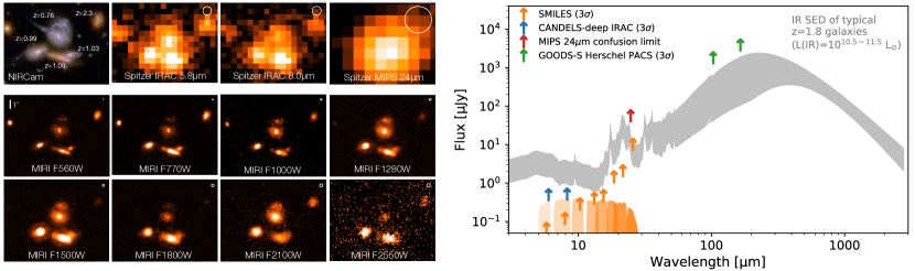
Figure 1: Power of SMILES in studying the mid-IR dust properties of galaxies at cosmic noon. Left: The top-left image shows a group of galaxies at $z\sim 0.7-2.3$ (matching the redshift range in this paper) in F444W/F200W/F090W NIRCam colors (JADES). The pre-JWST mid-IR view of these galaxies is shown in the top row from Spitzer IRAC and MIPS (GOODS survey; Dickinson & FIDEL Team 2007; Ashby et al. 2015). The bottom two rows show the mid-IR images with JWST MIRI at 5.6, 7.7, 10, 12.8, 15, 18, 21, and 25.5  $\mu$m (SMILES). The PSF sizes are shown with white circles in the corners (diameter of the circle is the FWHM). The unprecedented improvement of MIRI in spatial resolution (0.19 to 0.86^′′ from 5.6 to 25.5  $\mu$m) compared to that of IRAC (1.72 and 1.88^′′ at 5.8 and 8  $\mu$m) and MIPS 24  $\mu$m (6^′′) makes it possible to observe the mid-IR emission of individual typical galaxies at these redshifts. Right: The IR dust SEDs of typical galaxies at $z=1.8$ with IR luminosities of $10^{10.5}-10^{11.5}\,L_{\odot}$ (Rieke et al. 2009; corresponding to obscured SFRs of $\sim 5-50$  $M_{\odot}$/yr assuming the Kennicutt & Evans 2012 calibration) in grey shaded region, along with 3$\sigma$ sensitivity limits of the GOODS-S Herschel/PACS (green; Magnelli et al., 2013), Spitzer MIPS 24  $\mu$m confusion limit (red; 56 $\mu$Jy, Dole et al. 2004), Spitzer IRAC Channels 3 and 4 (blue; Guo et al., 2013), and the MIRI sensitivities of SMILES in $\sim 10-30$ min exposures (orange; Section 2.1). MIRI filter transmission curves are shown with orange shaded regions. The high sensitivity and multi-band capability of MIRI enables measurements and characterizations of IR emission of typical galaxies at cosmic noon.

2 Methods and Observations

2.1 SMILES survey (MIRI data)

This paper is based on the MIRI imaging survey of Systematic Mid-infrared Instrument Legacy Extragalactic Survey (SMILES). SMILES is a MIRI US-GTO program (PID 1207, PI: George Rieke) that surveys 34 arcmin² (using 15 MIRI pointings in a 3$\times$ 5 mosaic) centered in the Hubble Ultra Deep Field (HUDF; Beckwith et al. 2006). The survey is centered at 03h32m34.80s -27d48m32.60s and includes the eight broad bands of the MIRI Imager from 5.6 to 25.5 $\mu$m. A standard MIRI 4-point dither pattern was adopted to improve the PSF sampling and mitigate detector artifacts and cosmic-ray events. We used a FASTR1 readout pattern. Each pointing had a total science exposure time of 2.17 hours, divided over 8 bands. The exposure times per band were designed to optimize the detection of typical AGN and star-forming galaxies down to SFR$\sim 10$ $M_{\odot}$yr^-1 (see also Lyu et al., 2023). The observations were carried out in December 2022 and January 2023, which achieved 5$\sigma$ point source sensitivity of 0.11 $\mu$Jy (AB mag $=$ 26.3), 0.20 $\mu$Jy (25.6), 0.48 (24.7), 0.67 (24.3), 0.79 (24.2), 2.42 (22.9), 3.47 (22.6), and 16.91 (20.8) in F560W (754 s exposure time), F770W (866 s), F1000W (644 s), F1280W (755 s), F1500W (1121 s), F1800W (755 s), F2100W (2186 s), and F2550W (832 s). The achieved sensitivities are an order of magnitude deeper than the confusion limit of Spitzer/MIPS 24  $\mu$m (56 $\mu$Jy; Dole et al. 2004) at similar wavelengths. The optimal combination of depth, spatial resolution, coverage area, and multi-wavelength capabilities, makes SMILES well suited for investigating mid-IR dust emissions in galaxies during the cosmic noon epoch. In Figure 1, we show the advancement of this dataset compared to the existing IR data to study cosmic noon galaxies.

Data reduction

Data reduction of MIRI images was performed using the nominal JWST Pipeline released by the Space Telescope Science Institute (JWST Calibration Pipeline v1.10.0; Bushouse et al. 2023), using JWST Calibration Reference System (CRDS) jwst 1084.pmap, with two custom modifications on the background subtraction and astrometry, and a post-processing flux calibration correction on F560W and F770W (see below). After the astrometric and background corrections, the final MIRI mosaic is made through the Pipeline stage 3 with a pixel scale of 0.06”.

Background correction

MIRI photometry relies on background-limited sensitivity across all bands, but particularly at longer wavelengths where the thermal emission from the telescope is significant (Glasse et al., 2015; Rigby et al., 2023). The background imprints a large spatial gradient on the image (Dicken et al., in prep). In addition, in some cases there are tree-ring shaped features and striping along the detector columns and rows (Morrison et al., 2023) that can also be corrected for during the background subtraction step. Therefore, proper correction is crucial to reach maximum sensitivity. We adopt a custom background subtraction methodology that is explained in detail in Pérez-González et al. (2024). In brief, this routine is performed on the products of the calwebb image2 (cal files) step of the Pipeline. It combines the cal images taken in the same band from different pointings to create a “super-background”, departing from the routine in the JWST pipeline, which utilizes only the four dithers for each pointing. Through an iterative process, for each cal file, we mask out sources, large gradients, and striping using median filtering. This way, the “super-background” is constructed for each uncleaned cal file. Finally, a median subtraction is applied to remove any remaining background variation, usually caused by cosmic ray showers.

Astrometry correction

This step is done on the background-subtracted cal files, the output from the previous paragraph. The tweakreg step in the Pipeline (in stage 3) is designed to calculate the astrometry correction of the image. However, in the earlier versions it was designed for automated processing without a user input reference catalog. As the MIRI images do not cover an area of the sky large enough to contain a sufficient number of GAIA point sources, it is necessary to supply an external reference catalog made from the HST or NIRCam images in the field was necessary. We adopted the tweakwcs package with a custom routine outside of the Pipeline. We use the NIRCam F444W mosaic (JADES survey; registered to GAIA DR3) to correct the F560W image by creating matched catalogs of high S/N F444W and F560W sources. We use the registered F560W to correct F770W, and so on, up to F1500W. The F1500W is used to correct F1800W, F2100W, and F2550W images as their number of high S/N sources in each band are insufficient for independent corrections. The achieved astrometric accuracy is $0.01-0.02$” (1$\sigma$) in all filters except F2550W, which has a low number of high S/N sources and an astrometric accuracy of $\sim 0.04$”.

Flux calibration correction

After data reduction and photometry (see below), we realized the F560W and F770W flux measurements are systematically overestimated. This became apparent when the predicted F560W fluxes from full SED fitting to HST, NIRCam, and MIRI data (excluding F560W) of sources with spectroscopic redshifts were consistently lower than the observed F560W photometry. Moreover, we compared the photometry with Spitzer IRAC and found a similar systematic overestimation in MIRI photometry. Based on simulations of the PSF, we concluded that this is likely due to an underestimation of the cruciform spikes of the MIRI PSF (Gáspár et al., 2021) in the flux calibration step of the Pipeline (this is now updated in the Pipeline, see below). Therefore, we calculate correction factors by comparing the observed F560W and F770W fluxes with the predicted fluxes from best-fit SEDs of 25 isolated stars using ASTRODEEP photometry up to IRAC2 (Lyu et al., 2023). The correction factors of 1.26 and 1.04 are applied to the F560W and F770W Kron fluxes, respectively (see below for photometry). The absolute flux calibration was updated in the JWST Calibration Reference Data System (CRDS) after the current reductions on December 14, 2023, to better account for the cruciform effect and the time dependence of MIRI sensitivity (Gordon et al., in prep). The correction factors relevant for SMILES are 1.27 and 1.18 in F560W and F770W. While the F560W correction is in agreement with our calculations, the official new calibrations for F770W are higher than ours. However, since the presented work is not highly dependent on the F770W flux (rest-frame of $\sim 2.5-4.5$  $\mu$m), our results will be unchanged with either correction factor.

Photometry

MIRI source detection and photometric extraction were performed using a modified version of the JADES photometric pipeline (jades-pipeline, for the pipeline see Rieke et al. 2023; Robertson et al. 2023; for MIRI photometry see also Lyu et al. 2023). We briefly summarize the main points here: a detection and S/N map were constructed by stacking the F560W and F770W mosaics, which were then used to define an initial blended segmentation map down to a low threshold in source S/N. This segmentation map was then processed to optimally deblend sources and remove spurious noise spikes. The final segmentation map and detection image are then used to define source centroids and photometry is measured in all filters at these centroids. In this work, we adopt 2.5x scaled Kron photometry. As noted above, correction factors are applied to the flux calibration at F560W and F770W. Aperture corrections are determined as the fraction of flux outside a given Kron aperture based on empirical PSFs for F560W and F770W (using comissioning data PID 1028, Dicken et al. in prep, A. Gáspar, private communication) and model PSFs generated from WebbPSF (Perrin et al., 2014) for the other bands. Photometric uncertainties are derived by placing apertures at random positions on a masked mosaic, which accounts for correlated pixel noise. A more detailed description of the construction of the SMILES photometric catalog will be presented in the survey paper (Alberts et al., in prep).

2.1.1 JADES, JEMS, and HST data

We use deep NIRCam imaging data in multiple filters spanning 1-5  $\mu$m from the JWST Advanced Deep Extragalactic Survey (JADES) in GOODS-S (PID 1180 , PI: D. Eisenstein) and the medium bands of the JWST Extragalactic Medium-band Survey (JEMS, PID 1963, Williams et al. 2023). We refer to the JADES survey data release papers for further details on the observations and data reduction (Rieke et al., 2023; Eisenstein et al., 2023). In brief, JADES GOODS-S covers a total of 67 square-arcminutes. The survey has two tiers: i) Deep with 27 square-arcminutes in NIRCam F090W, F115W, F150W, F200W, F277W, F335M, F356W, F410M, and F444W bands, and ii) Medium with 40 square-arcminutes with the same filters, but without F335M. We also include NIRCam medium bands F210M, F430M, F460M, and F480M from the JEMS survey, where available.

We use Kron photometry from the custom-developed jades-pipeline (discussed in Section 2.1; Robertson et al., 2023; Rieke et al., 2023). Furthermore, we use the spectroscopic redshifts from JADES NIRSpec (Bunker et al., 2023), where available (Section 2.3.3). To cover the shorter wavelengths, we also include existing HST/ACS F435W, F606W, F775W, F814W, and F850LP data from the Hubble Legacy Fields (HLF) v2.0 (Illingworth et al., 2013), applying the same photometry jades-pipeline as for the NIRCam data.

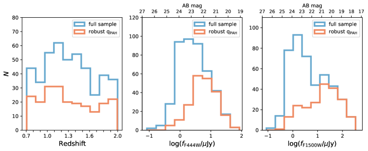
Figure 2: Distributions of redshift (left), F444W flux density (middle), and F1500W flux density (right) for the “full” sample ($N=443$) and the subsample with robust PAH mass fractions ($N=216$) defined as those with q_PAH error $<0.5\%$ or q_PAH parameter constrained by $>3\sigma$ from the SED fitting (Section 2.2). The sample is purely star-forming with AGN and quiescent galaxies removed (Section 2.2).

2.1.2 FRESCO data and redshifts

The field of SMILES is fully covered by the FRESCO-GOODS-S F444W grism survey (PID 1895, Oesch et al. 2023), which results in detection of Pa$\alpha$ at $z\sim 1.0-1.7$ and Pa$\beta$ at $z\sim 2.0-2.9$.

The details of the grism data reduction and extractions are in (Oesch et al., 2023). We extract the grism spectra for 1,296 MIRI-selected galaxies ($3\sigma$ detected in F560W or F770W) at $z=0.5-3.5$ based on existing spectroscopic redshifts from the literature and photometric redshifts based on HST/ACS$+$JADES/NIRCam. The extractions follow the standard continuum$+$contamination removal procedure explained in Oesch et al. (2023) and Kashino et al. (2023). The spectra are fit within $\Delta(z)=\pm 0.02(1+z_{\rm spec})$ for the objects with existing spec-$z$, otherwise within the lower and upper 68% quantiles of their photo-$z$. The redshift probability distributions are then calculated mainly based on the detections of Pa$\alpha$ at $z=1.07-1.66$, Pa$\beta$ at $z=2.03-2.88$, and/or Hei$\lambda 1083$, [Siii], [Sii], and higher order Paschen lines. We visually inspect all the 1D extractions, the line fits, and accordingly evaluate the quality of the redshift estimations. The final sample statistics are: 30% (386) have robust fits and redshifts, out of which 56% had prior spectroscopic redshifts; 50% (653) of the fits are unreliable (e.g., no line, incomplete spectral coverage, contamination from other sources, etc.); and 20% (257) are flagged as undetermined quality (noisy spectra, weak line or multiple lines that give different solutions). In total, 57% of the MIRI-selected sample (743 galaxies) have either a FRESCO redshift or other spectroscopic redshift (3DHST and other literature).

2.2 Final Sample

We start from the MIRI-selected sample (3$\sigma$ detected in F560W or F770W) and use the following criteria to define our final sample:

1. $z=0.7-2.0$ to ensure adequate PAH coverage by MIRI data

2. $3\sigma$ detection in at least one MIRI band longwards of 15 $\mu$m.

3. removal of quiescent galaxies based on their rest-frame $U-V$ and $V-J$ colors (following Equation 3 in Schreiber et al. 2015). For a cleaner selection, we also remove galaxies with specific SFR (sSFR, SFR/$M_{*}$ from SED modeling, see Section 2.3) $<10^{-10}$ yr^-1.

4. removal of objects with unusual/incorrect photometry from visual inspections of the SED fits.

This selection results in 443 galaxies. The stellar mass and SFR distribution is shown in Figure 6. Specifically for the PAH analysis in this work, we further limit the sample to those with “robust” PAH mass fraction (q_PAH, see Section 2.3.1). This category is defined as galaxies with either $>3\sigma$ q_PAH values or q_PAH error of less than 0.5%. The second condition allows the inclusion of near-zero PAH fractions that are still relatively robust. The rest of the sample is denoted as “low-confidence” q_PAH throughout the paper. The robust q_PAH sample has 216 objects. Figure 2 shows the distributions of redshift, F444W (tracing emission from old stellar populations) and F1500W (tracing dust/PAH emission) of the robust and full samples. The robust q_PAH sample is skewed towards brighter galaxies (and relatively more massive and dusty), by definition. Even though this subsample is biased, the separation is necessary to have a sample with reliable PAH fraction estimates. However, we show the results and trends for the low-confidence sample as well as the robust sample in the paper.

2.3 SED Fitting

We adopt the PROSPECTOR SED fitting code (Johnson et al., 2021) to fit the UV to mid-IR photometry. PROSPECTOR is a highly flexible SED fitting code that is based on Bayesian forward modeling and Monte Carlo sampling of the parameter space using FSPS stellar populations (Conroy, 2013). We adopt the “current” or “surviving” stellar mass throughout this paper, which takes into account losses throughout the evolution of stars in the galaxy via AGB winds, supernovae, etc. This is different from the mass of stars that are formed in the lifetime of the galaxy. In our sample, the ratio of the surviving to the formed stellar mass is on average 0.69 with a scatter of 0.04 (for a Chabrier IMF). Below, we first discuss the assumptions on modeling the dust emission (Section 2.3.1), then discuss the validity of the derived PAH fractions (Section 2.3.2). Finally, in Section 2.3.3, we discuss the remaining assumptions in the SED fitting.

2.3.1 Dust emission assumptions

The dust emission models in PROSPECTOR are based on the models of Draine & Li (2007). These models assume a mixture of amorphous silicate grains and carbonaceous grains with a distribution of grain sizes chosen to reproduce the wavelength dependence of the Milky Way (MW) extinction curve, while the silicate and carbonaceous content was constrained by the ISM gas phase depletion observations. The radiation field heating the dust is assumed to have a fixed shape (spectrum) of the local interstellar radiation field (Mathis et al., 1983), scaled by a dimensionless factor $U$. Three parameters of these models are free in the PROSPECTOR framework: q_PAH, fraction of the grain mass contributed by PAHs containing fewer than $10^{3}$ carbon atoms, U_min, the intensity of the diffuse ISM radiation field heating the dust, and $\gamma$, the fraction of dust mass exposed to the power-law distribution of starlight radiation intensities between U_min and U_max (($1-\gamma$) is the fraction of dust mass exposed to U_min).

In the absence of far-IR constraints, the IR parameters are constrained based on the energy balance assumption between the UV-near-IR dust attenuated luminosity and the re-emitted IR luminosity. Leja et al. (2017) experimented with the output with and without far-IR data on a large sample of local galaxies. They concluded that in the absence of far-IR constraints, it is critical to have tight priors on the shape of the far-IR emission to avoid unrealistically large uncertainties and potential systematic biases in SFR, $L_{\rm IR}$, and dust attenuation. Following their recommendation, we adopt a flat prior of $0.1<U_{\rm min}<15$ and $0.0<\gamma<0.15$. For the q_PAH parameter we adopt a flat prior of $0.4<{\rm q_{PAH}}<4.6$, as this is the range of q_PAH that the Draine & Li (2007) models are specifically constrained for. We derived q_PAH for a subsample of the galaxies with ALMA 1.1 and 3 mm observations and find no systematic offset between the derived values including and excluding the ALMA data, as explained in Section 2.3.2.

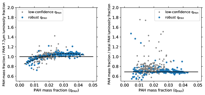
Figure 3: The ratio of the PAH-to-dust mass fraction to the PAH-to-total IR luminosity fraction versus the PAH mass fraction in our sample. Both quantities are derived from the Draine & Li (2007) models (Section 2.3). Robust q_PAH sample shows galaxies with q_PAH with $>3\sigma$ significance or less than 0.5% error (Section 2.2). Left: PAH luminosity fraction is defined as the ratio of the PAH 7.7  $\mu$m feature luminosity to total IR luminosity. Horizontal line is the unity line. The robust sample is fit with a polynomial function shown with a dashed curve (Equation 1). Right: PAH luminosity is the sum of the 3.3, 6.2, 7.7, 11.2, and 17  $\mu$m PAH features luminosities (Section 2.3.1). Horizontal line shows the median of the robust sample (0.68). Note that q_PAH is not in percentage units, unlike the other figures in this paper.

We note that the fraction of dust mass in PAHs used in this work, denoted as q_PAH, should be distinguished from the fraction of total IR luminosity in PAH bands. The two quantities are related to each other but not with a constant value as the light-to-mass ratio of dust is not a fixed value in the Draine & Li (2007) models (it is a function of radiation field intensity for the dust that produces the IR continuum and for PAHs, it depends on the stochastic heating). In Figure 3, we compare the two quantities for our sample. The PAH mass fraction is compared to the PAH luminosity fraction defined as either the ratio of PAH 7.7  $\mu$m feature ($F_{7.7}$, left panel) or total PAH luminosity (right panel) to total IR luminosity (integrated luminosity from 3 to 1100  $\mu$m). $F_{7.7}$ is calculated as the integrated PAH flux ($\int(F_{\lambda}-F^{\rm{continuum}}_{\lambda})\leavevmode\nobreak\ {\rm d}\lambda$) between 6.9 and 9.7 $\mu$m and is corrected for the continuum emission by assuming zero feature strength on either side of the feature at 6.9 and 9.7 $\mu$m, following the recipe of Draine et al. (2021). The total PAH luminosity is the sum of the luminosity of the 3.3, 6.2, 7.7, 11.2, and 17  $\mu$m features, measured in the same way as the 7.7  $\mu$m luminosity within the windows defined by Draine et al. (2021). As shown in the figure, the PAH mass fraction can be converted to the total PAH luminosity fraction by a factor of 0.68 (the median value of q_PAH to total PAH luminosity fraction), however there is a large scatter around this median value. The q_PAH to PAH 7.7  $\mu$m luminosity fraction is tighter, but the relation with q_PAH is not linear. We fit the relationship with a polynomial function:

$$\frac{{\rm q_{PAH}}}{F_{7.7}/F_{\rm TIR}}=-0.024\times{\rm q_{PAH}}^{2}+0.158\times{\rm q_{PAH}}+0.805,$$ (1)

where $F_{7.7}/F_{\rm TIR}$ is the PAH 7.7  $\mu$m to total IR luminosity fraction, and q_PAH is the fraction of PAH to dust mass. The q_PAH values presented in this work can be converted to the PAH 7.7  $\mu$m luminosity fraction using this equation, if needed.

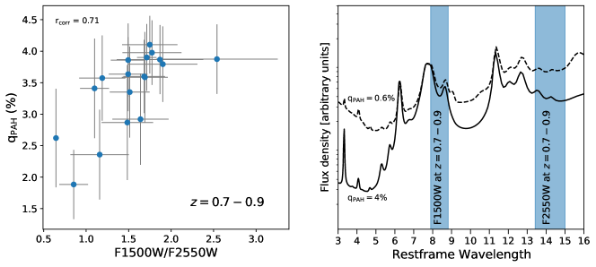
Figure 4: Left: PAH-to-dust mass fraction (q_PAH) versus 15 $\mu$m (F1500W) to 25.5 $\mu$m (F2550W) flux ratios for a sample of $z=0.7-0.9$ galaxies with significant ($>3\sigma$) detections in F1500W and F2550W. q_PAH is derived from PROSPECTOR (the Draine & Li 2007 models), while the flux ratio is an empirical tracer of PAH to warm dust emission, as shown in the right panel. The significant linear correlation of the two quantities (Pearson correlation coefficient of 0.71 with p-value = 0.001) indicates the validity of the estimated q_PAH values. Right: Two mid-IR spectra with a high PAH fraction (solid) and low PAH fraction (dashed), overlaid with the wavelength coverage of the F1500W and F2550W filters at $z=0.7-0.9$. In this redshift range, F1500W and F2550W filters trace the PAH dominated and non-PAH-dominated dust emission in star-forming galaxies, respectively. Therefore, their ratio is expected to correlate with PAH fraction.

2.3.2 How well is q_PAH constrained?

The majority of our sample does not have IR detections beyond MIRI. Therefore, the PAH mass fractions are inferred solely based on UV to mid-IR (MIRI) data. As a validity check for the derived q_PAH parameters, we perform two tests, as follows.

We compare the q_PAH values for a sample of 18 galaxies at $z=0.7-0.9$ that have significant ($>3\sigma$) detections at 15 and 25.5 $\mu$m. As shown in the right panel of Figure 4, $z=0.9$ is the highest redshift that our longest-wavelength band (F2550W) traces the part of the SED that is dominated by the continuum dust emission, and not that of PAHs. At $z=0.7-0.9$, the F1500W filter traces the $7-8$ $\mu$m PAH complex. Therefore, the ratio of F1500W to F2550W fluxes traces the PAH to warm dust emission, which, in theory, is expected to scale with the PAH-to-dust mass fraction (i.e., q_PAH). As shown in the left panel of Figure 4, the derived q_PAH values from the SED fits are highly correlated with the F1500W to F2550W flux ratio, with a Pearson correlation coefficient of 0.71 (p-value $\ll 1$).

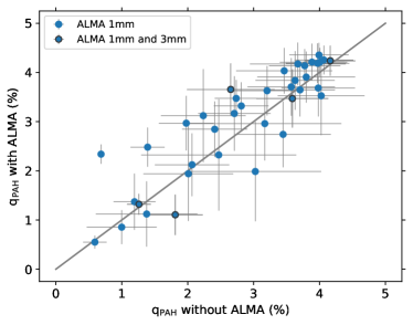
Figure 5: PAH to total dust mass fraction for the 38 galaxies with ALMA 1.1 mm detection (from the ASPECS survey; Walter et al., 2016). Five of them also have 3 mm detections. The axes show the derived q_PAH including and excluding the ALMA data points. Median of the q_PAH values without ALMA to those with ALMA data is 0.95, completely within the q_PAH uncertainty, indicating the q_PAH values inferred based on UV-to-MIRI data alone are robust.

As q_PAH depends on both the PAH mass and the mass of the other dust grains, the parameter may be uncertain in the absence of far-IR data. There are 38 SMILES galaxies with ALMA 1.1 mm (band 6) detection from one of the deepest ALMA extragalactic surveys, ASPECS (Walter et al., 2016). Five of these also have 3 mm detections (band 3). We compare the derived q_PAH of this sample including and excluding ALMA data in Figure 5. There is no systematic difference in q_PAH within the uncertainties. Given the luminosity range of these galaxies, this is in agreement with previous studies that showed PAHs as good tracers of IR luminosity in relatively bright (and non-ULIRG) galaxies (Reddy et al., 2012; Shipley et al., 2016). Therefore, we conclude that our derived q_PAH values are robust even without far-IR data under our fitting assumptions.

2.3.3 Other SED assumptions

We assume a delayed-$\tau$ star formation history with a flat age prior between 1 Myr to the age of the universe at the redshift of the galaxy. Stellar metallicity is free with a flat prior between $\log(Z/Z_{\odot})=-2.5-0.19$. For dust attenuation, we adopt a flexible attenuation curve that has its UV slope as a free parameter as parameterized in Kriek & Conroy (2013), with a flat prior between $-0.6$ to 0.3 for the multiplicative coefficient of the slope of the Calzetti et al. (2000) curve. We include AGN emission, even though the AGN fraction of our sample is very low, by definition of the sample (median of 0.05% AGN-to-bolometric stellar luminosity fraction). We assume a nebular emission model with flat priors in logarithmic space of gas-phase metallicity at $-2.0$ to 0.5 (relative to solar metallicity) and ionization parameter at $-4$ to $-1$. We include IGM absorption (Madau, 1995) with the optical depth scaling factor as a free parameter with a Gaussian prior centered at 1.0 and $\sigma=0.3$.

Redshift is fixed if the spectroscopic redshift is available from various non-JWST spectroscopic campaigns (compilations of Kodra et al. 2023, Bacon et al. 2023) or JWST JADES NIRSpec (Bunker et al., 2023) and FRESCO NIRCam grism (Oesch et al., 2023) surveys. In the absence of spec-$z$, the redshift parameter is left free with a a clipped-normal prior distribution centered at the photometric redshift and limits of the photo-$z$ uncertainty. The photo-$z$ is taken from the JADES photometric redshift catalog (Hainline et al., 2023), with typical uncertainties of $\Delta(z)/z=0.04-0.1$ (median of 0.06).

2.4 MIRI sizes

Dust sizes and surface areas are estimated from MIRI data as a proxy for where the bulk of stars are forming in galaxies. These measurements are later used to calculate SFR surface densities. We calculate dust sizes from MIRI F1500W images with 0.5” resolution, tracing rest-frame $5-9$  $\mu$m. The choice for F1500W filter to measure dust sizes is done as this filter provides a good compromise between wavelength and spatial resolution.

We use WebbPSF (Perrin et al., 2014) to model the F1500W PSF. We adopt a point-source model and a single-Sérsic model to fit the spatial profiles and estimate sizes. For a complete morphological analysis, more complicated models are required but for our current purposes these simple models provide reasonable sizes for the majority of the sample. Galaxies that are fit better (smaller reduced $\chi^{2}$) with a Sérsic model than the point-source model are considered spatially resolved. Sources that are best fit with the point source model or with a Sérsic profile but their half-light radius is smaller than the 50% encircled energy radius for the appropriate filter are considered unresolved. For the unresolved sources, we use the 50% encircled energy size of the PSF as an upper limit on their effective radius. We visually inspect all fits and remove the bad fits (e.g., if the source has signs of merger or nearby bright companions). This results in 105 F1500W good fits for extended objects in our sample.

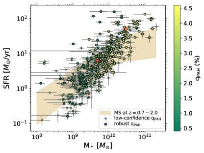
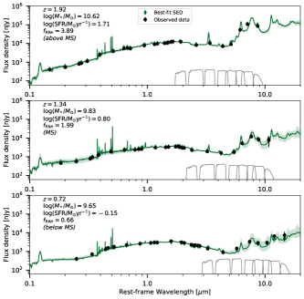
Figure 6: Left: SFR versus stellar mass of the sample. The sample is divided into those with robust and low-confidence PAH mass fractions (same as in Figure 2). The shaded region indicates star-forming main sequence at the redshift range of our galaxies, $z=0.7-2.0$, derived from the PROSPECTOR-inferred SFR and mass of Leja et al. (2022), same as the SFR and stellar masses inferred in this work. Three SED examples of the symbols with red edges are shown on the right. Right: Examples of the SEDs of three galaxies that are above, on, and below the main sequence, shown with the red edges in the left plot. The MIRI filter transmission curves are also shown. The wealth of data from HST, NIRCam, and MIRI provides robust SED fits for this sample at $z=0.7$ to 2.0.

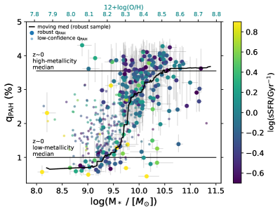
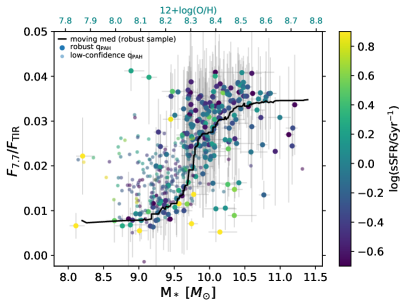
Figure 7: PAH mass fraction (left) and luminosity fraction (right) as a function of stellar mass. Moving median (black curve) is shown for the robust q_PAH sample (see Section 2.2 for the definition of samples), and all galaxies are color-coded by sSFR. In the left panel, vertical lines show the median PAH mass fractions of $z\sim 0$ galaxies with $12+\log{\rm{(O/H)}}$$<8.1$ and $>8.1$ from Draine et al. (2007). On the top x-axes, we also show the estimated metallicities from the O3N2-based mass-metallicity relation (MZR) of Topping et al. (2021) at $z\sim 1.5$, and assuming the Pettini & Pagel (2004) calibration. The $z\sim 0.7-2$ sample has a very similar q_PAH-metallicity behaviour to that inferred at $z\sim 0$.

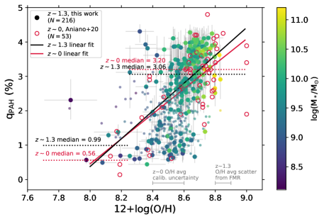
Figure 8: PAH mass fraction versus metallicity. Metallicity is derived from the fundamental metallicity relation (FMR) of Sanders et al. (2021). The robust and low-confidence q_PAH samples (Section 2.2) are shown with larger and smaller circles, respectively. The $z\sim 0$ data from Aniano et al. (2020) are shown in red. Following the analysis of Aniano et al. (2020), we fit both samples with a linear function, shown with solid lines (slopes of $3.63\pm 0.71$ and $4.04\pm 0.51$ and intercepts of $-28.60\pm 6.14$ and $-31.94\pm 4.38$ for the $z\sim 0$ and 1.3 sample, respectively). The medians of the two samples below and above $12+\log{\rm{(O/H)}}$$=8.25$ (dotted lines) are also shown. The two samples follow very similar trends. The average scatter in $12+\log{\rm{(O/H)}}$ from FMR (0.05 dex, see text) and the strong-line metallicity calibration uncertainty for the $z\sim 0$ sample (0.2 dex; Aniano et al. 2020) are shown in the bottom right. The error bars on the $z\sim 1.3$ data are the metallicity measurement uncertainties from the SFR and mass uncertainties. The linear fits (solid lines) have slopes of 3.6 and 3.4 for the $z\sim 0$ and 1.3 samples, respectively.

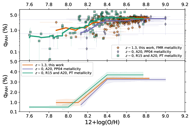
Figure 9: PAH mass fraction as a function of metallicity at $z\sim 1.3$ (this work) and $z\sim 0$ (Aniano et al., 2020; Rémy-Ruyer et al., 2015). Here, we only include the robust q_PAH sample at $z\sim 0.7-2.0$. Top: The $z\sim 1.3$ data presented in this work is shown with orange circles. The orange line shows the moving median. Metallicity of the $z\sim 1.3$ sample is estimated using the FMR relation of Sanders et al. (2021). The $z\sim 0$ data is shown for the PP04 metallicity calibrations of Aniano et al. (2020) (purple diamonds, and purple line for the moving median) and the PT metallicity calibrations of Aniano et al. (2020) and Rémy-Ruyer et al. (2015) (green squares, and the green line for the moving median). The Rémy-Ruyer et al. (2015) data extend the $z\sim 0$ sample to much lower metallicities. The two metallicity calibrations are systematically different (on average $\sim 0.2$ dex but can be up to 0.4 dex), therefore we show both for completeness. Bottom: Three-step fits (constant$+$linear$+$constant) to the moving median trends in the top panel. The shaded regions show the error in the mean in each consecutive bin of the moving median. Despite the uncertainties in metallicities, the overall q_PAH-metallicity behavior of the $z\sim 0$ and $z\sim 1.3$ samples are similar within the scatter.

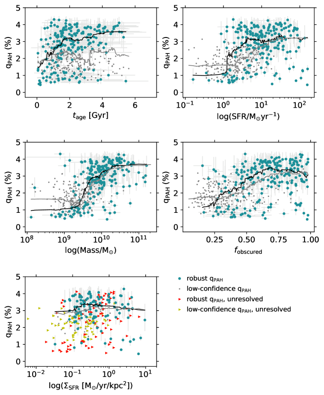
Figure 10: PAH mass fraction as a function of galaxy parameters. From top-left to bottom-right: age of the galaxy, SFR, stellar mass, obscured luminosity fraction, SFR surface density (using F1500W sizes). The robust sample is shown with teal color and the low-confidence sample with smaller grey symbols (see Section 2.2 for sample definitions). The moving medians of the full (robust$+$low-confidence) and robust samples are shown as grey and black curves, respectively. In the bottom row, the unresolved sources in F1500W images are shown with triangles as lower limits on SFR surface density. Among the parameters show, q_PAH has the strongest correlations with mass, age, and obscured luminosity fraction.

3 Evolution of PAH fraction

Figure 6 shows the full and the robust (q_PAH determined at $>3\sigma$) samples in the SFR-$M_{*}$ (star-forming main-sequence) diagram. The colors indicate the inferred q_PAH for the robust sample, which ranges from $\sim 0.5-4.5$%. The galaxies are representative of “main sequence” galaxies at these redshifts (Leja et al., 2022) and span a wide range in sSFR. Examples of the SED fits for three objects that are above, on, and below the main-sequence are shown in the right panels. In the following sections, we investigate the relationship between PAH fractions and galaxy parameters, and its evolution from $z\sim 2$ to $z\sim 0$.

3.1 PAH fraction versus stellar mass

In Figure 7, we show the relationship between stellar mass and q_PAH (left panel) and the 7.7  $\mu$m PAH luminosity fraction relative to total IR luminosity emission ($F_{7.7}/F_{\rm{TIR}}$; right panel). $F_{7.7}$ is the integrated PAH flux ($\int(F_{\lambda}-F^{\rm{continuum}}_{\lambda})\leavevmode\nobreak\ {\rm d}\lambda$) between 6.9 and 9.7 $\mu$m and is corrected for the continuum emission, following the recipe of Draine et al. (2021), and the total IR (TIR) power is the integrated emission ($\int F_{\lambda}\leavevmode\nobreak\ d\lambda$) from 3 to 1100 $\mu$m of the best-fit SED model.

The PAH “strength”, defined as either the PAH mass or emission fraction, is positively correlated with stellar mass with a correlation coefficient of $\rho_{\rm Pearson}=0.5$ for the robust q_PAH sample and 0.6 for the full sample (with p-values of $\ll 1$). We also estimate the gas-phase metallicity ($12+\log{\rm{(O/H)}}$) based on stellar masses and the $z\sim 1.5$ O3N2-based mass-metallicity relation (MZR) of Topping et al. (2021) and the Pettini & Pagel (2004) calibration, shown on the top axis of Figure 7. The median trend of q_PAH with the MZR-estimated metallicities closely resembles the local galaxies trend from Draine et al. (2007) (the horizontal lines in Figure 7-left). The two q_PAH median values of the local galaxies were reported at metallicities below and above $12+\log{\rm{(O/H)}}$$=8.1$. The rapid change of q_PAH happens at $\sim 0.1-0.2$ dex higher oxygen abundances in our $z\sim 1.3$ sample compared to that at $z\sim 0$. However, given the uncertainties in metallicity calibrations (see also the next section), we conclude that the behaviour of the $z\sim 1.3$ sample is consistent with that at $z\sim 0$.

There is a large scatter in q_PAH at intermediate masses, such that in the mass range of $\log(M_{*}/M_{\odot})\sim 9.5-10.5$, there are galaxies with q_PAH of $<0.5\%$ to $>4\%$. The majority of these galaxies seem to have young ages and high specific SFRs (sSFR). To better understand the physical process driving the scatter, we also calculate partial correlation coefficients between q_PAH, $M_{*}$, and a third galaxy parameter, including sSFR, SFR, age, optical depth, obscured SFR fraction, and SFR surface density. However, we do not find a significant secondary dependence on any of these parameters in the q_PAH-$M_{*}$ correlation of the robust sample. If we limit the sample to only q_PAH values with $>3\sigma$ significance, the specific SFR (sSFR) and age reduce the q_PAH-$M_{*}$ correlation coefficient of 0.4 to a partial coefficient of 0.25, indicating a potential secondary influence on the q_PAH-$M_{*}$ correlation, such that at a given stellar mass, galaxies with higher sSFR and younger ages have lower PAH strengths.

3.2 PAH fraction versus metallicity from $z\sim 0$ to 2

The relation between the PAH fraction and metallicity has been extensively studied in the local universe (Marble et al., 2010; Engelbracht et al., 2005; Madden et al., 2006; Smith et al., 2007; Galliano et al., 2008; Draine et al., 2007; Rémy-Ruyer et al., 2015; Aniano et al., 2020; Li, 2020; Chastenet et al., 2023) and also at cosmic noon (Shivaei et al., 2017, using Spitzer data). To investigate this relation with the deeper MIRI data at $z>0$, we estimate metallicities from the fundamental metallicity relation (FMR) between stellar mass, SFR, and metallicity. The FMR is shown to be established and invariant up to $z\sim 3$ (Cresci et al., 2019; Sanders et al., 2021). Sanders et al. (2021) estimated the scatter in $12+\log{\rm{(O/H)}}$ from FMR to be 0.06 dex at $z\sim 2.3$, and 0.04 dex at $z\sim 0$. This is typically smaller (or at most comparable) to the systematic uncertainty in strong-line metallicity calibrations (e.g., $\sim 0.2$ dex average systematic uncertainty between the Pettini & Pagel (2004) and the Pilyugin & Thuan (2005) calibrations in Aniano et al. (2020), see their Figure 1). We adopt the FMR presented in Sanders et al. (2021) to estimate metallicities from our mass and SFR values. The adopted FMR is in agreement with those derived from direct-method metallicities (Andrews & Martini, 2013) and also with the best-fit for local galaxies in Curti et al. (2020). The average measurement uncertainty of the inferred $12+\log{\rm{(O/H)}}$, propagated from the SFR and mass uncertainties, is 0.03 dex, comparable to the FMR scatter in $12+\log{\rm{(O/H)}}$.

We limit the $z\sim 0$ comparison samples to two studies that adopted, similar to this study, the Draine & Li (2007) models to derive q_PAH and have homogeneous metallicity calculations: Aniano et al. (2020) (hereafter, A20) and Rémy-Ruyer et al. (2015) (hereafter, R15). A20 used two strong-line metallicity calibrations for the KINGFISH sample: 1) the “PT” or Pilyugin & Thuan (2005) method, adopted from Moustakas et al. (2010), and 2) the “PP04” or Pettini & Pagel (2004) based on [Nii]/H$\alpha$. They showed that the two metallicities can differ by as much as 0.4 dex (on average $\sim 0.2$ dex), reflecting the large uncertainty in the calibrations. R15 incorporated the Dwarf Galaxy Survey (DGS; Madden et al. 2013) into the KINGFISH which extended the sample to lower metallicities. They adopted the PT metallicity calibration.

Figure 8 shows the q_PAH trend with metallicity. There is a positive correlation (Pearson $\rho=0.55$ with p-value $\ll 1$) with a large scatter at high metallicities. The trend is very similar to the $z\sim 0$ trend from A20 (assuming their preferred PP04 metallicity). A20 approximated the q_PAH-metallicity behaviour by both a linear function and a step function. The median values below and above their threshold metallicity, $12+\log{\rm{(O/H)}}$$\sim 8.25$, and the slopes of the linear fits ($3.6\pm 0.7$ and $4.0\pm 0.5$ at $z\sim 0$ and 1.3, respectively) for the two samples suggest a non-evolving PAH fraction-metallicity relation from $z\sim 0-2$.

In Figure 9 (top panel), we compare our results with the $z\sim 0$ data over a wider range of metallicities by combining both the A20 and R15 data (using the PT metallicity). The q_PAH values of R15 extend to larger values compared to A20 and ours, because they set a higher upper limit for the q_PAH prior in their fittings. We also include A20 data for the PP04 metallicity, for completeness. To interpret and compare the datasets, we adopt a moving (running) median to smooth the data without assuming a parametric functional form a priori. All three trends show a constant low ($\lesssim 1\%$) q_PAH at low metallicities ($12+\log{\rm{(O/H)}}$$\lesssim 8.1-8.2$ or $\sim 0.3\,Z_{\odot}$ assuming $12+\log{\rm{(O/H)}}$$=8.69$ for Solar metallicity; Asplund et al. 2009), then a linear increase of q_PAH with metallicity that ends with a plateau (q_PAH $\sim 3.4\%$) at $12+\log{\rm{(O/H)}}$$\gtrsim 8.4$ ($\gtrsim 0.5\,Z_{\odot}$). We show the fits to the moving medians in the lower panel of Figure 9. The constant q_PAH at high metallicities confirms the successful usage of PAH strengths as IR luminosity and obscured SFR indicators for moderately massive and metal-rich galaxies based on local calibrations (e.g., Calzetti et al., 2007; Shipley et al., 2016). Our findings are also in general agreement with Marble et al. (2010) based on the $z\sim 0$ SINGS data, who found a linear relation between PAH luminosity fraction and metallicity. These observations show that, at least up to $z\sim 2$, metallicity is a good indicator of the ISM properties that affect the balance between the formation and destruction of PAHs in star-forming galaxies, and the responsible processes maintain a constant PAH abundances of $\sim 3.4$% above a metallicity of $\sim 0.5\,Z_{\odot}$.

Below $\sim 0.5\,Z_{\odot}$, we see that there is a linear decrease of the PAH fraction, which has a similar slope between the $z\sim 0$ and 1.3 samples. This universal PAH fraction-metallicity relation can potentially be calibrated to estimate the metallicities of metal-poor galaxies at high redshifts using IR imaging surveys alone. The source of the decreasing PAH fraction with decreasing metallicity can be explained by the destruction of PAHs at low metallicities, either through radiative destruction in less shielded low-metallicity environments (Madden et al., 2006; Hunt et al., 2010; Narayanan et al., 2023), or supernova shocks (Seok et al., 2014). Some studies also explain it by insufficient production of PAHs due to a delayed injection into the ISM by AGB stars (Galliano et al., 2008) or more efficient production at high metallicities through shattering of large grains (Seok et al., 2014). Future cosmological simulations with on-the-fly dust evolution simulations can shed light on the complex interplay of the formation and destruction processes of these grains in the ISM.

3.3 PAH fraction and other galaxy parameters

In Figure 10 we show q_PAH as a function of other galaxy parameters: age, SFR, stellar mass, obscured luminosity fraction ($f_{\rm obscured}$), and SFR surface density ($\Sigma_{\rm SFR}$). Obscured luminosity fraction is calculated as the ratio of the dust-obscured UV (1550Å) luminosity to the intrinsic UV luminosity (see Section 4). Sizes are calculated in the F1500W filter, tracing rest-frame 5 to 9  $\mu$m dust emission, for galaxies with spatially resolved profiles (see Section 2.4). In the literature, $\Sigma_{\rm SFR}$ is often calculated based on the area derived from a shorter-wavelength size measurement that is not a good proxy for where the bulk of the stars are forming. Here, surface area is based on dust sizes (from F1500W) that closely reflects the star forming region, and hence, the resulting SFR surface densities are more reliable.

We show the moving medians for the robust (black curve) and the full sample (grey curve), which includes the robust sample, in Figure 10. In the robust sample, q_PAH correlates with age, stellar mass, and obscured fraction. The q_PAH-mass correlation is the strongest among these, and is likely a byproduct of the mass-metallicity relation (as discussed in the previous sections). The correlation with age can be expected as a stellar evolutionary effect if the AGB stars are the primary production channel of PAHs (Galliano et al., 2008; Li, 2020) and, in fact, it is also seen at $z\sim 2$ from MIPS data (Shivaei et al., 2017). However, this correlation disappears when the full sample is considered. The correlation with obscured fraction is interesting as it may suggest PAH destruction due to reduced shielding by dust grains in systems with low obscured fractions. We also note the lack of a significant correlation with SFR surface densities for the spatially resolved galaxies, which may suggest that the fraction of PAH-to-total dust mass is insensitive to the star formation intensity. Even including lower limits on SFR surface density for the unresolved sources (triangles in Figure 10) does not suggest a correlation with SFR surface density. Further analysis of this trend using size measurements from other filters that have higher resolution but still trace the dust emission will be done in a future work.

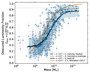
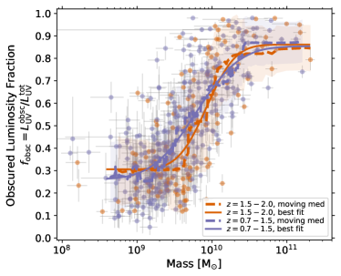
Figure 11: Obscured luminosity fraction as a function of stellar mass for the full sample (left) and separated by redshift (right). Obscured fraction is defined as the obscured UV to total (intrinsic) UV luminosity at 1550 Å, inferred from the best-fit UV-to-IR SEDs. We show the moving median (dashed thick lines), moving weighted-average (dotted line) and best-fit curve (solid lines) to the samples at $M_{*}>4\times 10^{8}$ $M_{\odot}$, where the data is mass-complete. In the left panel, we also show the Whitaker et al. (2017) fit to $z=0.5-2.5$ with an orange curve. The Whitaker et al. (2017) study was based on Spitzer/MIPS data with a wider area but biased to more obscured systems. Our weighted-average trend is also dominated by the heavily obscured systems, and therefore similar to the (Whitaker et al., 2017) curve. However, the median trend that is more representative of the full population captured by the deeper MIRI data (relative to the MIPS data) is systematically lower. Furthermore, as shown in the right panel, there is no redshift evolution in this relation in our sample.

4 Dust obscured luminosity fraction

The largest uncertainty in measuring SFR is the fraction of dust-obscured star formation. The most reliable and direct method of accounting for the dust-obscured fraction is observing the dust thermal emission in IR. With Spitzer and Herschel, both sensitivity and confusion noise limitations have impeded our ability to calculate the obscured SFR in typical and low-mass galaxies at $z\sim 1$ and above without relying on stacking many galaxies. MIRI directly traces mid-IR PAH emission up to $z\sim 3$ ($z\sim 2$ with the more sensitive shorter-wavelength bands). Even though converting mid-IR emission to total IR luminosity is model-dependent, its uncertainty is typically lower than that affecting the UV slope methods for moderately and highly obscured galaxies (e.g., Shivaei et al., 2020). In this section, we estimate the obscured luminosity fraction from our UV-to-mid-IR SED fits and study its variation as a function of stellar mass and SFR surface density.

In the previous section, we showed that the PAH fraction reaches a constant average value at metallicities above $\sim 0.5Z_{\odot}$, and hence using PAH luminosity to estimate total IR luminosity and obscured SFR is robust in this regime. However, as the PAH fraction changes at lower metallicities, instead of a simple PAH-to-IR luminosity conversion, we adopt the full UV-to-mid-IR energy-balanced SED fits to derive the obscured fraction as the ratio of obscured to intrinsic (total) UV luminosity at 1550 Å: $f_{\rm obsc}=L^{\rm obscured}_{\rm UV}/L^{\rm intrinsic}_{\rm UV}=1-(L^{\rm unattenuated}_{\rm UV}/L^{\rm intrinsic}_{\rm UV})$, where the unattenuated UV luminosity is directly constrained by the observed photometry at rest-frame UV and the intrinsic UV luminosity is estimated from the dust-free (intrinsic) best-fit SED model. Our choice of using the UV luminosity to estimate the obscured fraction is because of its multiple implications for high-redshift studies that often only have UV data, but we note that the fractions are in very close agreement with total IR to unattenuated UV luminosity (as expected). Converting the luminosity fractions to SFR fractions require additional conversions of the luminosities to SFRs, which we decide to avoid in the current paper to mitigate uncertainties.

4.1 Relationship between obscured fraction and mass

As most of the metals in the ISM are depleted onto dust grains that attenuate starlight, it is expected that obscured luminosity fraction (ratio of attenuated to intrinsic luminosity) correlates with metallicity, and hence stellar mass (e.g., Reddy et al., 2010; Whitaker et al., 2017).

In Figure 11, the obscured fraction is shown as a function of stellar mass. We investigate the average shape and scatter of the relationship at $M_{*}>4\times 10^{8}$ $M_{\odot}$, where the sample is complete. The mass completeness is estimated based on the detection limits of 5.6  $\mu$m and 15  $\mu$m data and assuming a mass-to-light ratio of 0.6 at 2.2 $\mu$m (McGaugh & Schombert, 2014). To study the average trend, we fit the data in three ways: a moving median function, the functional form of $f_{\rm obsc}$-$M_{*}$ suggested by Whitaker et al. (2017),

$$f_{\rm obscured}=\frac{1}{1+a\leavevmode\nobreak\ e^{b\log(M_{*}/M_{\odot})}},$$ (2)

where $f_{\rm obscured}$ is the obscured fraction, and $a$ and $b$ are the fit parameters, and the following function that best matches the moving median trend:

$$f_{\rm obsc}=\dfrac{(f_{\rm max}-f_{\rm min})}{2}\times\left({\rm erf}\left(\dfrac{\log(M_{*}/M_{\odot})-\mu}{\sqrt{2}\leavevmode\nobreak\ \sigma}\right)+1\right)+f_{\rm min},$$ (3)

where erf is the error function, and $f_{\rm max}$, $f_{\rm min}$, $\mu$, and $\sigma$ are the fitting parameters. Using an Orthogonal Distance Regression (ODR) fitting procedure (python scipy.odr), considering the uncertainties on both the obscured fraction and mass, the fit using Equation 2 matches the Whitaker et al. (2017) curve closely. However, our fit is highly biased by the few highly obscured galaxies with very small uncertainties. The moving (running) weighted-average curve, where the weight is the inverse square of uncertainty in $f_{\rm obsc}$, also shows how this small population of highly obscured galaxies bias the fit (dotted curve in Figure 11). The running median (dashed curve) and the Equation 3 fit (black line) better represent the behaviour of $f_{\rm obsc}$ as a function of mass. The best fit parameters are listed in Table 1.

Table 1: Best-fit parameters of $f_{\rm obscured}-M_{*}$ for the full sample in Equation 3

$f_{\rm max}$	$f_{\rm min}$	$\sigma$	$\mu$
$0.873\pm 0.015$	$0.273\pm 0.015$	$0.441\pm 0.043$	$9.856\pm 0.026$

We do not see any significant redshift evolution in this relation, as shown in the right panel of Figure 11, in agreement with the findings of Whitaker et al. (2017) that at a fixed mass the obscured fraction is constant from $z\sim 0.5$ to 2.5. Based on our best-fit curve (Eq. 3) that matches the moving median, on average, the UV luminosity is dominantly obscured ($f_{\rm obsc}$$>50\%$) above the stellar mass of $\sim 5\times 10^{9}$  $M_{\odot}$. Interestingly, owing to the large scatter in $f_{\rm obsc}$ at any mass, there are galaxies with dominantly obscured emission even down to $M_{*}\sim 5\times 10^{8}$  $M_{\odot}$. We investigate the scatter in $f_{\rm obsc}$ at fixed mass in the next section. Above the stellar mass of $2\times 10^{10}$  $M_{\odot}$, more than 80% of the emission is obscured. However, the SMILES survey is likely not representative of the population of heavily obscured (and rare) galaxies owing to its relatively small area.

Whitaker et al. (2017) studied the Spitzer/MIPS samples and found that the $f_{\rm obscured}$-$M_{*}$ relation does not change from $z=0$ to $2.5$. They fit the UV-near-IR photometry with Bruzual & Charlot (2003) models and used the Dale & Helou (2002) template to convert 24 $\mu$m flux densities to total IR luminosities. Then assuming the Kennicutt (1998) and Bell et al. (2005) calibrations, they converted UV and IR luminosities to SFRs to estimate $f_{\rm obsc}=\frac{\rm SFR_{IR}}{\rm SFR_{IR}+SFR_{UV}}$. While the two relationships are in relatively good agreement within the scatter of the relation in Figure 11, there are a few differences between the Whitaker et al. (2017) study and this work that contribute to the mild disagreement between the two relationships. Whitaker et al. (2017) used a single log-averaged IR template to convert PAH luminosity to total IR luminosity across their sample at $z\sim 0.5-2.5$. While this assumption works for galaxies at high metallicities (and high masses), as we showed in the previous section, below $\sim 0.5Z_{\odot}$ the PAH fraction decreases uniformly from $z\sim 0-2$. Therefore, using the high-metallicity end calibrations would overestimate the IR luminosities at lower metallicities (and masses). Additionally, the different area and sensitivity of SMILES compared to the MIPS/Spitzer surveys can play a role in the observed discrepancy between this study and the Whitaker et al. (2017) study. SMILES is more sensitive to less obscured galaxies at a fixed mass relative to the MIPS samples. In fact, the fit to our data using the Whitaker et al. (2017) formalism and an ODR fitting procedure (i.e., taking into account the uncertainties on $f_{\rm obsc}$) closely follows the Whitaker et al. (2017) curve. This is because a few highly obscured galaxies with very low $f_{\rm obsc}$ uncertainties dominate the fit – a similar bias that a MIPS-based sample would have. Furthermore, SMILES has a smaller area compared to the Spitzer MIPS surveys, and hence, is likely missing a (more rare) population of massive and highly attenuated galaxies.

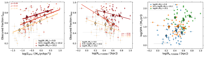
Figure 12: Obscured luminosity fraction as a function of $\Sigma_{\rm SFR}$ (using F1500W sizes) and F1500W effective radius (middle) for the F1500W spatially resolved sample (the filter FWHM is 0.5 arcsec). At a given mass, $f_{\rm obsc}$ increases with $\Sigma_{\rm SFR}$ and decreases with rest-frame mid-IR (dust) radii. Right panel shows SFR versus F1500W size for the same sample. The near constant SFR with ${\rm R_{e,F1500W}}$ in each mass bin indicates that the relationship between $f_{\rm obsc}$ and size is independent of SFR. Individual measurements are shown with small symbols and color-coded in three stellar mass bins with the same number of galaxies, shown in the legend. In each mass bin, average values in bins of the parameter on the x-axis are shown with larger symbols with the corresponding shape and color of the mass bin. Pearson correlation coefficients ($\rho$) are shown in the corners of the plots with corresponding colors of each mass bin. Linear fits to the average values of $f_{\rm obsc}$ versus $\log$($\Sigma_{\rm SFR}$) are shown in the left panel. The fit parameters are in Table 2.

4.2 Scatter in $f_{\rm obsc}$-$M_{*}$ and relationship with $\Sigma_{\rm SFR}$

As mentioned in the previous section, there is a large scatter in $f_{\rm obsc}$ at a given mass, such that there are galaxies with significant obscured UV emission down to stellar masses of $\sim 5\times 10^{8}$  $M_{\odot}$. The scatter in the obscured fraction at a given mass increases from 0.1 dex at $M_{*}\sim 10^{11}$  $M_{\odot}$ to $\sim 0.5$ dex at $M_{*}\sim 10^{9}$  $M_{\odot}$. We calculate secondary correlations in the $f_{\rm obsc}-M_{*}$ relation with sSFR, age, and SFR surface density using partial correlation coefficients. The surface density is measured using dust sizes from F1500W data (Section 2.4). In those calculations the sample is limited to galaxies with spatially resolved disks in F1500W. The spatially-resolved sample is limited to galaxies with $M_{*}>10^{9.5}$  $M_{\odot}$, and inevitably biased against the extremely compact star forming galaxies. The stellar mass distribution of the spatially-resolved sample above $M_{*}>10^{9.5}$  $M_{\odot}$ is very similar to that of the parent sample with 50% of the spatially resolved sample at $M_{*}<10^{10.2}$  $M_{\odot}$. Among the sSFR, age, and SFR surface density parameters, we find a relatively strong correlation between the obscured fraction and SFR surface density at a fixed stellar mass, but no significant correlations with age and SFR at constant mass.

Figure 12 shows the obscured fraction versus SFR surface density ($\Sigma_{\rm SFR}$, left) and F1500W effective radii (middle). $\Sigma_{\rm SFR}$ is calculated using dust surface area (at rest-frame $8-9$  $\mu$m) that closely traces the active star forming region. We divide the sample in three stellar mass bins to investigate the trend at a fixed mass. The average values are shown with large symbols in the figure.

There is a clear correlation between $f_{\rm obsc}$ and $\Sigma_{\rm SFR}$ at all masses with Pearson correlation coefficient of $\sim 0.5$ (p-value $\ll 1$). We fit the average trends in each mass bin with a linear function. As expected, the overall normalization increases with increasing mass – i.e., as shown in the previous figures, $f_{\rm obsc}$ increases with increasing mass. However, not only does $f_{\rm obsc}$ clearly increase with $\Sigma_{\rm SFR}$ (and decreases with size) at a given mass, but the rate at which $f_{\rm obsc}$ increases with $\Sigma_{\rm SFR}$ (i.e., the slope) appears to be similar across the mass range of the sample. The fit parameters are presented in Table 2. We discuss the possible explanation of this behaviour in the next Section. While the overall trend with size (effective radius) is consistent, the slope of the $f_{\rm obsc}$-size relation varies among the three mass bins and the evolutionary behaviour is not as clear as with $\Sigma_{\rm SFR}$. We also note that the width of the $f_{\rm obsc}$ distribution decreases as the mass increases, as shown with the errorbars on the average values in Figure 12. The standard deviation of $f_{\rm obsc}$ in the highest $\Sigma_{\rm SFR}$ bin from low to high mass is 0.20, 0.15, 0.07, respectively.

The right panel of Figure 12 confirms that the $f_{\rm obsc}$ increasing trend with $\Sigma_{\rm SFR}$ is not a byproduct of increasing SFR. While there is a general correlation between SFR and size for the full sample, the average SFR does not vary with size in the fixed mass ranges. Therefore, the underlying cause of $f_{\rm obsc}$ dependence on $\Sigma_{\rm SFR}$ at a given mass is the compactness of the star forming region, and not only an increase in the rate of star formation.

Table 2: Fit parameters of the linear fits in Figure 12.

$N$	Mass range [$\log(M_{*}/M_{\odot})$]	$f_{\rm obscured}$-$\log(\Sigma_{\rm SFR}/M_{\odot}{\rm yr^{-1}kpc^{-2}})$		$f_{\rm obscured}$-$\log({\rm R_{e,F1500W}/kpc})$
		slope	intercept	slope	intercept
50	$<9.9$	0.15$\pm 0.03$	0.647$\pm 0.017$	$-0.29\pm 0.08$	$0.668\pm 0.034$
43	$9.9-10.2$	0.14$\pm 0.02$	0.722$\pm 0.011$	$-0.52\pm 0.08$	$0.899\pm 0.036$
38	$>10.2$	0.12$\pm 0.02$	0.791$\pm 0.006$	$-0.23\pm 0.04$	$0.904\pm 0.023$

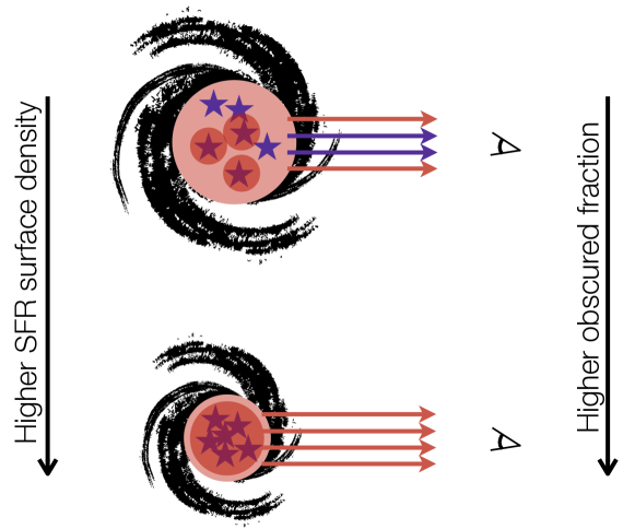
Figure 13: A cartoon illustrating a physical explanation of the correlation between $f_{\rm obsc}$ and star forming compactness. Stars are shown in blue. Diffuse ISM dust is shown with light red and the “birth cloud” dust with higher column density is shown with darker red color. Schematically, less and more dust-obscured light (i.e., obscured by the low and high column density dust, respectively) are shown with blue and red arrows, respectively, reaching to the observer on the right. Extended galaxies have a range of dust-star geometries, while compact galaxies contain most of their stellar population in the core with high dust covering fraction, resulting in most of the emitted starlight being obscured by dust.

4.3 Morphological evolution and obscured fraction

Using submm/mm data for samples with generally much higher stellar masses and SFRs than presented here, studies have shown that star formation occurs in more compact regions compared to the stellar mass sizes (e.g., Murphy et al., 2017; Jiménez-Andrade et al., 2021; Hodge et al., 2016; Elbaz et al., 2018; Fujimoto et al., 2017; Rujopakarn et al., 2019). Additionally, it has been argued that starburst galaxies on the main-sequence with particularly short depletion timescales exhibit higher SFR surface densities with more compact mm dust emission (Elbaz et al., 2018; Gómez-Guijarro et al., 2022) and radio emission (Jiménez-Andrade et al., 2019), and hotter dust (Gómez-Guijarro et al., 2022) compared to other main-sequence galaxies at the same mass and redshift. In the regime of lower SFR surface density ($\log(\Sigma_{\rm SFR}/M_{\odot}{\rm yr^{-1}}\leavevmode\nobreak\ {\rm kpc^{-2}})\sim-1$ to 1 ) and mass ($\log(M_{*}/M_{\odot})\sim 9.5$ to 11), we observe the same relation for purely star-forming galaxies (no AGN contamination) that PAH dust sizes are more compact with higher SFR surface densities at a fixed mass (right panel of Figure 12).

We also see that the obscured emission is more dominant in compact galaxies with higher $\Sigma_{\rm SFR}$. This observed trend is illustrated by a simple cartoon in Figure 13. For an extended star forming galaxy the dust-star geometry is more complex: some population of stars are only affected by the diffuse ISM dust, while others can be trapped in their birthcloud dust and highly attenuated. If the star forming region is compressed into a small area, the galaxy will have a more homogeneous dust distribution with higher covering fraction that attenuates most of the light emitted from the stars. Hence, the obscured fraction of the emitted light is higher in galaxies with compact star forming regions. This explanation works for closed-box systems. However, strong outflows and feedback may clear pathways through the ISM of the compact star forming regions and expose the starlight without attenuation. This may explain the larger variation of $f_{\rm obsc}$ in the low mass bins at any $\Sigma_{\rm SFR}$: low-mass galaxies have highly stochastic star formation histories (Hopkins et al., 2014), and massive stars produced in the vigorous starbursts can destroy their birth clouds via feedback (e.g. winds, supernovae; Naidu et al. 2022) to make sightlines clear of dust. This will generate a diversity of $f_{\rm obsc}$ from galaxy to galaxy at low masses, while in massive galaxies dust stays in the compact core with high covering fraction. In our data, the scatter (standard deviation) of $f_{\rm obsc}$ in the lowest mass bin is $15-20$% at a fixed $\Sigma_{\rm SFR}$ and decreases to $8-12$% in the highest mass bin.

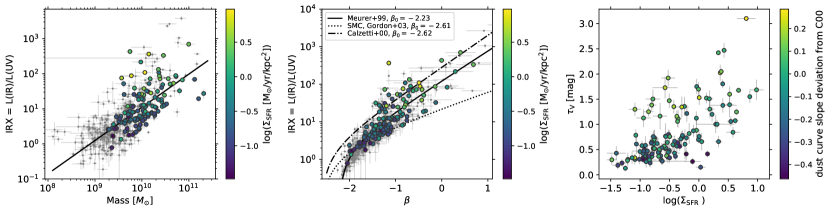
Figure 14: Left and Middle: IRX (ratio of IR to UV 1550 Å luminosity) as a function of stellar mass (left) and UV stellar continuum slope (middle). Galaxies with spatially resolved morphology in F1500W are color coded by their $\Sigma_{\rm SFR}$. A linear fit to $\log({\rm IRX})-\log(M_{*}/M_{\odot})$ is shown in the left panel (slope of $0.96\pm 0.06$ and intercept of $-8.47\pm 0.61$). In the middle panel, we show three IRX-$\beta$ relations in the literature adopted from Reddy et al. (2018) assuming a constant star formation history and an age of 100 Myr for stellar populations: the original Meurer et al. (1999) relation, the starburst curve of Calzetti et al. (2000) and the SMC curve of Gordon et al. (2003) assuming 0.14 Solar metallicity. A higher metallicity system will result in a redder intrinsic UV slope ($\beta_{0}$), shifting the curves to the right of the diagram (e.g., the Calzetti curve for a 1.4 $Z_{\odot}$ population and $\beta_{0}=-2.4$ resembles the Meurer et al. 1999 curve). Galaxies with higher $\Sigma_{\rm SFR}$ at a given mass or $\beta$ have higher IRX and a shallower attenuation curve. Right: $V$-band dust optical depth versus $\Sigma_{\rm SFR}$, color coded with the attenuation curve slope defined as the deviation from the Calzetti et al. (2000) (the formalism of Kriek & Conroy 2013), where zero is the Calzetti curve slope. The two parameters are highly correlated with $\rho=0.65$ (p-value $\ll 1$). The shallower attenuation curve of galaxies with high IRX at a given mass/$\beta$ can be explained by the radiative transfer effects that are a result of their high $\Sigma_{\rm SFR}$: higher optical depths and lower fractions of unobscured evolved stars.

The relationship of obscured fraction with compactness of star forming region can also explain the spread in the locus of galaxies in the IRX-$\beta$ diagram. The IRX-$\beta$ relation is an empirical calibration of UV stellar continuum slope ($\beta$) based on the ratio of IR to unobscured UV luminosity (IRX; Meurer et al. 1999). The location of galaxies in this diagram depends on the slope of the attenuation curve in the UV and the intrinsic UV slope (e.g., Reddy et al., 2018; Shivaei et al., 2020; Salim & Narayanan, 2020; Hamed et al., 2023). Figure 14 shows the distribution of our sample in the IRX-mass and IRX-$\beta$ diagrams. Galaxies with higher $\Sigma_{\rm SFR}$ at a given mass or $\beta$ have higher IRX, and preferentially shallower attenuation curves similar to that of the Calzetti et al. (2000) curve (middle panel; similar trends are also seen at $z\sim 0$, Johnson et al. 2007). The preference for shallower curves is potentially due to both a higher average optical depth and a lower fraction of unobscured evolved stars. Radiative transfer models have shown that a high dust optical depth flattens the dust attenuation curve (Chevallard et al., 2013) and the right panel of Figure 14 shows that $\Sigma_{\rm SFR}$ in our sample is correlated with the dust optical depth (Pearson $\rho=0.65$ with p-value $\ll 1$). Additionally, as shown in the schematic Figure 13, galaxies with more concentrated star forming regions (higher $\Sigma_{\rm SFR}$) have lower fraction of evolved stars unobscured by dust, as these stars would not have sufficient time to migrate away from their dusty birth clouds. This dust-star geometrical effect also tends to flatten the dust attenuation curve of galaxies in which the evolved stars dominate the optical luminosity (Narayanan et al., 2018). The inclination (axis ratio) of galaxies can also play a role in the observed trends, which will be investigated in future studies.

5 Conclusions

In this study, we use SMILES, the largest 5-25  $\mu$m MIRI survey in the first two observing cycles of JWST, to study the dust obscured and PAH grain properties of 443 galaxies at $z=0.7-2.0$ (with a median redshift of $z\sim 1.3$). The exceptional sensitivity, angular resolution, and mid-IR wavelength coverage offered by SMILES enables unambiguous detection of dust emission from star-forming regions in galaxies, reaching an order of magnitude lower mass and SFR than was achievable with JWST’s predecessor, Spitzer. Augmented by the deep NIRCam (JADES) and HST (CANDELS) data in GOODS-S, we perform SED fitting on the extremely well covered photometry spanning from rest-frame UV to mid-IR. We study the PAH to dust mass fractions (q_PAH) and dust-obscured fraction of UV luminosity ($f_{\rm obsc}$) in relation to galaxy parameters such as stellar mass, metallicity, and SFR surface density. The sample contains main-sequence galaxies spanning a range from $\sim 10^{8.4}-10^{11.3}$  $M_{\odot}$. Our key findings are summarized below.

• We find a strong correlation between the mass fraction of dust in PAHs (i.e., PAH mass fraction or q_PAH) and stellar mass. Similar correlation is seen between the PAH luminosity fraction relative to the total IR luminosity and mass. This correlation positions the q_PAH value of the majority of galaxies at $z\sim 1.3$ between the median values of low- and high-metallicity galaxies at $z\sim 0$ (Draine et al., 2007).

• Using the fundamental metallicity relation (FMR), we estimate the gas metallicity of the sample and compare the q_PAH-metallicity relation at $z\sim 1.3$ with that at $z\sim 0$. Despite the uncertainties in the $z\sim 0$ metallicities due to strong-line calibrations ($\sim 0.2$ dex, Aniano et al. 2020), compared to the $\sim 0.05$ dex metallicity scatter from FMR), we observe a strong agreement in the q_PAH-metallicity trends from $z\sim 0$ to 2. In this relationship, q_PAH remains relatively constant at $\sim 3.4$% above $\sim 0.5\,Z_{\odot}$, confirming the reliability of PAH luminosity as a robust calibrator for estimating total IR luminosity (and similarly, PAH mass to dust mass) in metal-rich galaxies. Below $0.5\,Z_{\odot}$, the PAH fraction declines sharply, reaching a very low value of $<1$% at metallicities below $0.3\,Z_{\odot}$. This redshift-invariant nature of the q_PAH-metallicity relation below $\sim 0.5\,Z_{\odot}$ could potentially serve as a basis for calibrating the PAH luminosity fraction as a metallicity indicator in this range. This would be an efficient way of estimating metallicities from relatively cost-effective imaging surveys, with MIRI applicable up to $z\sim 2$ and potential future far-IR probes such as SPICE (Urry et al. 2023, Bonato et al., in prep) or PRIMA (Moullet et al., 2023) extending capabilities to $z\sim 7$.

• We observe a strong correlation between the fraction of obscured UV emission (ratio of obscured to total UV luminosity) and stellar mass that does not change with redshift. Galaxies with stellar masses above $10^{9.6}$  $M_{\odot}$ have, on average, more than half of their light obscured by dust. In the stellar mass range of $\sim 10^{8.5}$ to $10^{11}$  $M_{\odot}$, the obscured fraction increases from $\sim 15\%$ to more than $90\%$.

• We determine dust sizes using F1500W images, which capture the $\sim 5-8.8$  $\mu$m dust and PAH emission within the redshift range of $z=0.7-2$. The spatial resolution of MIRI allows us to obtain sizes of galaxies at stellar masses $\sim 10^{9-11}$  $M_{\odot}$ (the median mass within the spatially resolved sample is $10^{10}$  $M_{\odot}$). Our findings indicate that, at a given mass, galaxies with compact dust regions (indicative of active star formation) exhibit higher SFR surface densities ($\Sigma_{\rm SFR}$). This suggests shorter depletion timescales in compact galaxies. Additionally, at the same mass, galaxies with higher $\Sigma_{\rm SFR}$ also exhibit higher obscured luminosity fractions. However, among lower mass galaxies, there is a broader range of $f_{\rm obsc}$ at a fixed $\Sigma_{\rm SFR}$.

• We explain the observed correlation between $f_{\rm obsc}$ and $\Sigma_{\rm SFR}$ at a constant mass by attributing it to the increase in dust covering fraction as the star-forming region becomes more compact. Simultaneously, the observed increase in the scatter of $f_{\rm obsc}$ at low masses compared to that in more massive bins can be attributed to the more bursty nature of star formation in lower mass galaxies. Feedback mechanisms may contribute to the wider range of dust covering fractions at low masses for a given $\Sigma_{\rm SFR}$.

• Similarly, we find that for a given mass or UV continuum slope ($\beta$), galaxies with higher attenuation quantified by the IRX (IR to unobscured UV luminosity) parameter tend to possess higher $\Sigma_{\rm SFR}$, positioning them within the region of the IRX-$\beta$ diagram that aligns with shallower attenuation curves. Such shallow attenuation curves may arise from both elevated average dust optical depths and a compact dust-star geometry (with reduced fraction of unobscured evolved stars) at high SFR surface densities.

We are just at the beginning of an exciting journey with MIRI to unveil the properties of dust beyond the local universe, at an unexplored SFR-mass regime. In the future, larger samples can help to solidify the trends presented here. Additionally, more sophisticated spatial analysis of the mid-IR data, as unbiased probes of intense star formation, will be invaluable in shedding light on the morphological evolution of galaxies.

References

- Álvarez-Márquez et al. (2023) Álvarez-Márquez, J., Labiano, A., Guillard, P., et al. 2023, A&A, 672, A108
- Andrews & Martini (2013) Andrews, B. H. & Martini, P. 2013, ApJ, 765, 140
- Aniano et al. (2020) Aniano, G., Draine, B. T., Hunt, L. K., et al. 2020, ApJ, 889, 150
- Armus et al. (2023) Armus, L., Lai, T., U, V., et al. 2023, ApJ, 942, L37
- Ashby et al. (2015) Ashby, M. L. N., Willner, S. P., Fazio, G. G., et al. 2015, ApJS, 218, 33
- Asplund et al. (2009) Asplund, M., Grevesse, N., Sauval, A. J., & Scott, P. 2009, Annual Review of Astronomy and Astrophysics, 47, 481
- Bacon et al. (2023) Bacon, R., Brinchmann, J., Conseil, S., et al. 2023, A&A, 670, A4
- Bakes & Tielens (1994) Bakes, E. L. O. & Tielens, A. G. G. M. 1994, ApJ, 427, 822
- Barrera et al. (2023) Barrera, N. F., Fuentealba, P., Muñoz, F., Gómez, T., & Cárdenas, C. 2023, MNRAS, 524, 3741
- Beckwith et al. (2006) Beckwith, S. V. W., Stiavelli, M., Koekemoer, A. M., et al. 2006, AJ, 132, 1729
- Bell et al. (2005) Bell, E. F., Papovich, C., Wolf, C., et al. 2005, ApJ, 625, 23
- Boschman et al. (2015) Boschman, L., Cazaux, S., Spaans, M., Hoekstra, R., & Schlathölter, T. 2015, A&A, 579, A72
- Bruzual & Charlot (2003) Bruzual, G. & Charlot, S. 2003, MNRAS, 344, 1000
- Bunker et al. (2023) Bunker, A. J., Cameron, A. J., Curtis-Lake, E., et al. 2023, arXiv e-prints, arXiv:2306.02467
- Bushouse et al. (2023) Bushouse, H., Eisenhamer, J., Dencheva, N., et al. 2023, JWST Calibration Pipeline
- Calzetti et al. (2000) Calzetti, D., Armus, L., Bohlin, R. C., et al. 2000, ApJ, 533, 682
- Calzetti et al. (2007) Calzetti, D., Kennicutt, R. C., Engelbracht, C. W., et al. 2007, ApJ, 666, 870
- Cardelli et al. (1989) Cardelli, J. A., Clayton, G. C., & Mathis, J. S. 1989, ApJ, 345, 245
- Chabrier (2003) Chabrier, G. 2003, PASP, 115, 763
- Chastenet et al. (2023) Chastenet, J., Sutter, J., Sandstrom, K., et al. 2023, ApJ, 944, L11
- Chevallard et al. (2013) Chevallard, J., Charlot, S., Wandelt, B., & Wild, V. 2013, MNRAS, 432, 2061
- Conroy (2013) Conroy, C. 2013, Annual Review of Astronomy and Astrophysics, 51, 393
- Cresci et al. (2019) Cresci, G., Mannucci, F., & Curti, M. 2019, A&A, 627, A42
- Curti et al. (2020) Curti, M., Mannucci, F., Cresci, G., & Maiolino, R. 2020, MNRAS, 491, 944
- Dale & Helou (2002) Dale, D. A. & Helou, G. 2002, ApJ, 576, 159
- Dickinson & FIDEL Team (2007) Dickinson, M. & FIDEL Team. 2007, in Bulletin of the American Astronomical Society, Vol. 39, American Astronomical Society Meeting Abstracts, 822
- Dickinson et al. (2003) Dickinson, M., Giavalisco, M., & GOODS Team. 2003, in The Mass of Galaxies at Low and High Redshift, ed. R. Bender & A. Renzini, 324
- Dole et al. (2006) Dole, H., Lagache, G., Puget, J. L., et al. 2006, A&A, 451, 417
- Dole et al. (2004) Dole, H., Rieke, G. H., Lagache, G., et al. 2004, ApJS, 154, 93
- Draine et al. (2007) Draine, B. T., Dale, D. A., Bendo, G., et al. 2007, ApJ, 663, 866
- Draine & Li (2007) Draine, B. T. & Li, A. 2007, ApJ, 657, 810
- Draine et al. (2021) Draine, B. T., Li, A., Hensley, B. S., et al. 2021, ApJ, 917, 3
- Eisenstein et al. (2023) Eisenstein, D. J., Johnson, B. D., Robertson, B., et al. 2023, arXiv e-prints, arXiv:2310.12340
- Elbaz et al. (2011) Elbaz, D., Dickinson, M., Hwang, H. S., et al. 2011, A&A, 533, A119
- Elbaz et al. (2018) Elbaz, D., Leiton, R., Nagar, N., et al. 2018, A&A, 616, A110
- Engelbracht et al. (2005) Engelbracht, C. W., Gordon, K. D., Rieke, G. H., et al. 2005, ApJL, 628, L29
- Fujimoto et al. (2017) Fujimoto, S., Ouchi, M., Shibuya, T., & Nagai, H. 2017, ApJ, 850, 83
- Galliano et al. (2008) Galliano, F., Dwek, E., & Chanial, P. 2008, ApJ, 672, 214
- Gardner et al. (2023) Gardner, J. P., Mather, J. C., Abbott, R., et al. 2023, PASP, 135, 068001
- Gáspár et al. (2021) Gáspár, A., Rieke, G. H., Guillard, P., et al. 2021, PASP, 133, 014504
- Glasse et al. (2015) Glasse, A., Rieke, G. H., Bauwens, E., et al. 2015, PASP, 127, 686
- Gómez-Guijarro et al. (2022) Gómez-Guijarro, C., Elbaz, D., Xiao, M., et al. 2022, A&A, 659, A196
- Gordon et al. (1997) Gordon, K. D., Calzetti, D., & Witt, A. N. 1997, ApJ, 487, 625
- Gordon et al. (2003) Gordon, K. D., Clayton, G. C., Misselt, K. A., Landolt, A. U., & Wolff, M. J. 2003, ApJ, 594, 279
- Guo et al. (2013) Guo, Y., Ferguson, H. C., Giavalisco, M., et al. 2013, ApJS, 207, 24
- Hainline et al. (2023) Hainline, K. N., Johnson, B. D., Robertson, B., et al. 2023, arXiv e-prints, arXiv:2306.02468
- Hamed et al. (2023) Hamed, M., Pistis, F., Figueira, M., et al. 2023, A&A, 679, A26
- Helou et al. (2001) Helou, G., Malhotra, S., Hollenbach, D. J., Dale, D. A., & Contursi, A. 2001, ApJL, 548, L73
- Hodge et al. (2016) Hodge, J. A., Swinbank, A. M., Simpson, J. M., et al. 2016, ApJ, 833, 103
- Hopkins et al. (2014) Hopkins, P. F., Keres, D., Oñorbe, J., et al. 2014, MNRAS, 445, 581
- Hunt et al. (2016) Hunt, L., Dayal, P., Magrini, L., & Ferrara, A. 2016, MNRAS, 463, 2002
- Hunt et al. (2010) Hunt, L. K., Thuan, T. X., Izotov, Y. I., & Sauvage, M. 2010, ApJ, 712, 164
- Illingworth et al. (2013) Illingworth, G. D., Magee, D., Oesch, P. A., et al. 2013, APJS, 209, 6
- Jiménez-Andrade et al. (2019) Jiménez-Andrade, E. F., Magnelli, B., Karim, A., et al. 2019, A&A, 625, A114
- Jiménez-Andrade et al. (2021) Jiménez-Andrade, E. F., Murphy, E. J., Heywood, I., et al. 2021, ApJ, 910, 106
- Johnson et al. (2021) Johnson, B. D., Leja, J., Conroy, C., & Speagle, J. S. 2021, ApJS, 254, 22
- Johnson et al. (2007) Johnson, B. D., Schiminovich, D., Seibert, M., et al. 2007, ApJS, 173, 392
- Kashino et al. (2023) Kashino, D., Lilly, S. J., Matthee, J., et al. 2023, ApJ, 950, 66
- Kennicutt (1998) Kennicutt, R. C. 1998, Annual Review of Astronomy and Astrophysics, 36, 189
- Kennicutt & Evans (2012) Kennicutt, R. C. & Evans, N. J. 2012, Annual Review of Astronomy and Astrophysics, 50, 531
- Kennicutt et al. (2009) Kennicutt, Jr., R. C., Hao, C.-N., Calzetti, D., et al. 2009, ApJ, 703, 1672
- Kirkpatrick et al. (2023) Kirkpatrick, A., Yang, G., Le Bail, A., et al. 2023, ApJ, 959, L7
- Kodra et al. (2023) Kodra, D., Andrews, B. H., Newman, J. A., et al. 2023, ApJ, 942, 36
- Kriek & Conroy (2013) Kriek, M. & Conroy, C. 2013, ApJL, 775, L16
- Lagache et al. (2004) Lagache, G., Dole, H., Puget, J. L., et al. 2004, ApJS, 154, 112
- Le Floc’h et al. (2005) Le Floc’h, E., Papovich, C., Dole, H., et al. 2005, ApJ, 632, 169
- Leja et al. (2017) Leja, J., Johnson, B. D., Conroy, C., van Dokkum, P. G., & Byler, N. 2017, ApJ, 837, 170
- Leja et al. (2022) Leja, J., Speagle, J. S., Ting, Y.-S., et al. 2022, ApJ, 936, 165
- Li (2020) Li, A. 2020, Nature Astronomy, 4, 339
- Lin et al. (2024) Lin, Y.-W., Wu, C. K. W., Ling, C.-T., et al. 2024, MNRAS, 527, 11882
- Lyu et al. (2023) Lyu, J., Alberts, S., Rieke, G. H., et al. 2023, arXiv e-prints, arXiv:2310.12330
- Madau (1995) Madau, P. 1995, ApJ, 441, 18
- Madden et al. (2006) Madden, S. C., Galliano, F., Jones, A. P., & Sauvage, M. 2006, A&A, 446, 877
- Madden et al. (2013) Madden, S. C., Rémy-Ruyer, A., Galametz, M., et al. 2013, PASP, 125, 600
- Magnelli et al. (2011) Magnelli, B., Elbaz, D., Chary, R. R., et al. 2011, A&A, 528, A35
- Magnelli et al. (2023) Magnelli, B., Gómez-Guijarro, C., Elbaz, D., et al. 2023, A&A, 678, A83
- Magnelli et al. (2013) Magnelli, B., Popesso, P., Berta, S., et al. 2013, A&A, 553, A132
- Marble et al. (2010) Marble, A. R., Engelbracht, C. W., van Zee, L., et al. 2010, The Astrophysical Journal, 715, 506
- Mathis et al. (1983) Mathis, J. S., Mezger, P. G., & Panagia, N. 1983, A&A, 128, 212
- McGaugh & Schombert (2014) McGaugh, S. S. & Schombert, J. M. 2014, AJ, 148, 77
- Meurer et al. (1999) Meurer, G. R., Heckman, T. M., & Calzetti, D. 1999, ApJ, 521, 64
- Morrison et al. (2023) Morrison, J. E., Dicken, D., Argyriou, I., et al. 2023, PASP, 135, 075004
- Moullet et al. (2023) Moullet, A., Kataria, T., Lis, D., et al. 2023, arXiv e-prints, arXiv:2310.20572
- Moustakas et al. (2010) Moustakas, J., Kennicutt, Robert C., J., Tremonti, C. A., et al. 2010, ApJS, 190, 233
- Murphy et al. (2017) Murphy, E. J., Momjian, E., Condon, J. J., et al. 2017, ApJ, 839, 35
- Naidu et al. (2022) Naidu, R. P., Matthee, J., Oesch, P. A., et al. 2022, MNRAS, 510, 4582
- Narayanan et al. (2018) Narayanan, D., Conroy, C., Davé, R., Johnson, B. D., & Popping, G. 2018, ApJ, 869, 70
- Narayanan et al. (2023) Narayanan, D., Smith, J. D. T., Hensley, B. S., et al. 2023, ApJ, 951, 100
- Oesch et al. (2023) Oesch, P. A., Brammer, G., Naidu, R. P., et al. 2023, MNRAS, 525, 2864
- Peeters et al. (2004) Peeters, E., Spoon, H. W. W., & Tielens, A. G. G. M. 2004, ApJ, 613, 986
- Pérez-González et al. (2024) Pérez-González, P. G., Barro, G., Rieke, G. H., et al. 2024, arXiv e-prints, arXiv:2401.08782
- Pérez-González et al. (2005) Pérez-González, P. G., Rieke, G. H., Egami, E., et al. 2005, ApJ, 630, 82
- Perrin et al. (2014) Perrin, M. D., Soummer, R., Choquet, É., et al. 2014, in Society of Photo-Optical Instrumentation Engineers (SPIE) Conference Series, Vol. 9143, Space Telescopes and Instrumentation 2014: Optical, Infrared, and Millimeter Wave, ed. J. Oschmann, Jacobus M., M. Clampin, G. G. Fazio, & H. A. MacEwen, 914309
- Pettini & Pagel (2004) Pettini, M. & Pagel, B. E. J. 2004, MNRAS, 348, L59
- Pilyugin & Thuan (2005) Pilyugin, L. S. & Thuan, T. X. 2005, ApJ, 631, 231
- Reddy et al. (2012) Reddy, N., Dickinson, M., Elbaz, D., et al. 2012, ApJ, 744, 154
- Reddy et al. (2010) Reddy, N. A., Erb, D. K., Pettini, M., Steidel, C. C., & Shapley, A. E. 2010, ApJ, 712, 1070
- Reddy et al. (2018) Reddy, N. A., Oesch, P. A., Bouwens, R. J., et al. 2018, ApJ, 853, 56
- Reddy et al. (2008) Reddy, N. A., Steidel, C. C., Pettini, M., et al. 2008, ApJS, 175, 48
- Rémy-Ruyer et al. (2015) Rémy-Ruyer, A., Madden, S. C., Galliano, F., et al. 2015, A&A, 582, A121
- Rieke et al. (2009) Rieke, G. H., Alonso-Herrero, A., Weiner, B. J., et al. 2009, ApJ, 692, 556
- Rieke et al. (2015) Rieke, G. H., Wright, G. S., Böker, T., et al. 2015, PASP, 127, 584
- Rieke et al. (2004) Rieke, G. H., Young, E. T., Engelbracht, C. W., et al. 2004, ApJS, 154, 25
- Rieke et al. (2023) Rieke, M. J., Robertson, B., Tacchella, S., et al. 2023, ApJS, 269, 16
- Rigby et al. (2023) Rigby, J. R., Lightsey, P. A., García Marín, M., et al. 2023, PASP, 135, 048002
- Robertson et al. (2023) Robertson, B., Johnson, B. D., Tacchella, S., et al. 2023, arXiv e-prints, arXiv:2312.10033
- Rujopakarn et al. (2019) Rujopakarn, W., Daddi, E., Rieke, G. H., et al. 2019, ApJ, 882, 107
- Rujopakarn et al. (2013) Rujopakarn, W., Rieke, G. H., Weiner, B. J., et al. 2013, ApJ, 767, 73
- Salim & Narayanan (2020) Salim, S. & Narayanan, D. 2020, arXiv e-prints, arXiv:2001.03181
- Sanders et al. (2021) Sanders, R. L., Shapley, A. E., Jones, T., et al. 2021, ApJ, 914, 19
- Sandstrom et al. (2023) Sandstrom, K. M., Koch, E. W., Leroy, A. K., et al. 2023, ApJ, 944, L8
- Schreiber et al. (2015) Schreiber, C., Pannella, M., Elbaz, D., et al. 2015, A&A, 575, A74
- Seok et al. (2014) Seok, J. Y., Hirashita, H., & Asano, R. S. 2014, Monthly Notices of the Royal Astronomical Society, 439, 2186
- Shen et al. (2023) Shen, L., Papovich, C., Yang, G., et al. 2023, ApJ, 950, 7
- Shipley et al. (2016) Shipley, H. V., Papovich, C., Rieke, G. H., Brown, M. J. I., & Moustakas, J. 2016, ApJ, 818, 60
- Shivaei et al. (2020) Shivaei, I., Darvish, B., Sattari, Z., et al. 2020, ApJ, 903, L28
- Shivaei et al. (2017) Shivaei, I., Reddy, N. A., Shapley, A. E., et al. 2017, ApJ, 837, 157
- Shivaei et al. (2015a) Shivaei, I., Reddy, N. A., Steidel, C. C., & Shapley, A. E. 2015a, ApJ, 804, 149
- Smith et al. (2007) Smith, J. D. T., Draine, B. T., Dale, D. A., et al. 2007, ApJ, 656, 770
- Thrower et al. (2012) Thrower, J. D., Jørgensen, B., Friis, E. E., et al. 2012, ApJ, 752, 3
- Tielens (2008) Tielens, A. G. G. M. 2008, ARA&A, 46, 289
- Topping et al. (2021) Topping, M. W., Shapley, A. E., Sanders, R. L., et al. 2021, MNRAS, 506, 1237
- Urry et al. (2023) Urry, C. M., Bonato, M., Leisawitz, D., et al. 2023, in AAS/High Energy Astrophysics Division, Vol. 55, AAS/High Energy Astrophysics Division, 103.78
- Walter et al. (2016) Walter, F., Decarli, R., Aravena, M., et al. 2016, ApJ, 833, 67
- Weingartner & Draine (2001a) Weingartner, J. C. & Draine, B. T. 2001a, ApJ, 548, 296
- Whitaker et al. (2017) Whitaker, K. E., Pope, A., Cybulski, R., et al. 2017, ApJ, 850, 208
- Whitaker et al. (2012b) Whitaker, K. E., van Dokkum, P. G., Brammer, G., & Franx, M. 2012b, ApJL, 754, L29
- Williams et al. (2023) Williams, C. C., Tacchella, S., Maseda, M. V., et al. 2023, ApJS, 268, 64
- Wolfire et al. (1995) Wolfire, M. G., Hollenbach, D., McKee, C. F., Tielens, A. G. G. M., & Bakes, E. L. O. 1995, ApJ, 443, 152
- Wright et al. (2023) Wright, G. S., Rieke, G. H., Glasse, A., et al. 2023, PASP, 135, 048003
- Xie & Ho (2019) Xie, Y. & Ho, L. C. 2019, ApJ, 884, 136