Frobenius light cone and the shift unitary

Abstract

We bound the time necessary to implement the shift unitary on a one-dimensional ring, both using local Hamiltonians and those with power-law interactions. This time is constrained by the Frobenius light cone; hence we prove that shift unitaries are parametrically harder to implement than preparing long-range Bell pairs for sufficiently small power-law exponent. We note an intriguing similarity between the proof of our results, and the hardness of preparing symmetry-protected topological states with symmetry-preserving Hamiltonians.

1 Introduction

The past decade has seen an enormous advance in our understanding of the limitations of spatial locality in many-body physics Lieb and Robinson (1972); Hastings and Koma (2006); Nachtergaele and Sims (2006); Wang and Hazzard (2020); Friedman et al. (2022), including in systems with power-law interactions Foss-Feig et al. (2015); Gong et al. (2017); Tran et al. (2019); Else et al. (2020); Guo et al. (2020); Chen and Lucas (2019); Kuwahara and Saito (2020); Tran et al. (2020); Kuwahara and Saito (2021a); Chen and Lucas (2021); Tran et al. (2021a) and bosons Jünemann et al. (2013); Kuwahara and Saito (2021b); Yin and Lucas (2022); Kuwahara et al. (2022); Faupin et al. (2022a, b); Lemm et al. (2023): see Chen et al. (2023a) for a recent review. These works often generalize the Lieb-Robinson Theorem Lieb and Robinson (1972), which constrains commutators between space-time distant local operators:

$$\lVert[A_{x}(t),B_{0}]\rVert\leq C(x,t).$$ (1)

By getting tight bounds on $C(x,t)$, we can show that e.g. the time it takes to perform state transfer between sites $x$ and 0 is at least as large as the smallest time $\tau$ for which $C(x,\tau)=2$ Bravyi et al. (2006). For many of the Lieb-Robinson bounds recently discovered, optimal protocols exist which demonstrate their tightness Eldredge et al. (2017); Tran et al. (2021b); Hong and Lucas (2021); Kuwahara et al. (2022).

It is also known that Lieb-Robinson bounds can be parametrically weak at bounding certain tasks. In theories with power-law interactions with a certain range of exponents, this was first emphasized in Tran et al. (2020), where it was noted that being able to implement a “background-independent state transfer” that transfers Pauli operators:

$$X_{0}(t)=X_{r},$$ (2)

is parametrically harder than performing state transfer between sites 0 and $r$. Note that these two tasks are not equivalent: fast state transfer protocols indeed rely on knowing the state of other qubits, whereas any protocol obeying (2) does not care about the state of any particular qubit. The authors of Tran et al. (2020) thus said that there was a “hierarchy of light cones”, with differing “light cones” (i.e. bounds on the time needed by an optimal protocol) for different tasks. The state transfer protocol of (2) is constrained by the “Frobenius light cone”, which is parametrically slower than the Lieb-Robinson one in power-law interacting systems Chen and Lucas (2021).

1.1 The shift unitary

This paper is about another task which we will prove is parametrically harder to perform in systems with power-law interactions: implementing the shift unitary on a one-dimensional ring of $R$ sites. We define the shift unitary $U_{\mathrm{sh}}$ as:

$$U_{\mathrm{sh}}^{\dagger}A_{x}U_{\mathrm{sh}}=A_{x+1}$$ (3)

for any single-qubit operator $A$. Here and below, site indices $x$ are integers modulo $R$. Our goal is to constrain the time necessary to implement $U_{\mathrm{sh}}$ using a local Hamiltonian protocol. Defining

$$U=\mathcal{T}\mathrm{e}^{-\mathrm{i}\int\mathrm{d}tH(t)},$$ (4)

subject to locality and boundedness constraints on $H(t)$, we will see that it can take a parametrically long time in system size to obtain $U=U_{\mathrm{sh}}$.

The shift unitary is an example of a quantum cellular automaton (QCA), which refers to any unitary operator with a strict light cone, meaning that $C(x,t)=0$ for large enough values of $x$ Farrelly (2020). In Gross et al. (2012), the authors (GNVW) showed that all QCA can be written as a composition of a finite-depth quantum circuit and a translation operator. The net flow of information of generated by the translation is a discrete invariant captured by the GNVW index of a QCA. This index is formally defined in terms of operator algebras on an infinite lattice, but it can also be understood in finite systems using tensor network methods Cirac et al. (2017) or entropic measures Duschatko et al. (2018); Gong et al. (2021). The index theory shows that any QCA with a non-zero index cannot be implemented as a finite-depth quantum circuit Gross et al. (2012). Indeed, the simplest implementation of the shift unitary requires a circuit of SWAP gates whose depth grows linearly in system size.

It is not a priori clear whether the index theory of QCA carries over to the case where interactions are only approximately locality-preserving, corresponding to light cones with decaying tails. This case is important since it is true for generic time evolutions generated by quasi-local Hamiltonians. In Ranard et al. (2022), the authors showed that the index theory is indeed well-defined even for approximately locality-preserving unitaries, such that QCA of non-zero index like $U_{\mathrm{sh}}$ cannot be implemented in finite time even with Hamiltonians having power-law decaying interactions (for large enough powers). However, the authors of Ranard et al. (2022) note that their technique is only applicable to strictly infinite-sized systems. One of the goals of this paper is to explain a few simple ways to prove the impossibility of easily implementing the shift on a finite ring.

1.2 Main result

The set-up of this paper is as follows. We consider a one-dimensional ring graph, where vertices are labeled by $\mathbb{Z}_{N}$. We place a qubit on every site of the ring graph, such that the quantum mechanical Hilbert space $\mathcal{H}=(\mathbb{C}^{2})^{\otimes N}$. The distance between vertices $x,y\in\mathbb{Z}_{N}$ is

$$\mathsf{d}(x,y)=\min(|y-x|,N-|y-x|).$$ (5)

For technical ease later, we focus on the case $N=4L$, but as our results are interesting in the large $N$ limit, this restriction could be easily relaxed. The induced distance between two sets $S,S^{\prime}$ is

$$\mathsf{d}(S,S^{\prime}):=\min_{x\in S,y\in S^{\prime}}\mathsf{d}(x,y).$$ (6)

The complement of a set $S$ is denoted by $S^{\rm c}$. For operator $A\in\mathrm{End}(\mathcal{H})$, $\mathrm{supp}(A)\subseteq\mathbb{Z}_{N}$ denotes the sites on which it acts non-trivially.

The main result of this paper is the following theorem:

Theorem 1.1.

Let $H(t)$ be a 2-local Hamiltonian on the ring:

$$H(t)=\sum_{\{x,y\}\subset\mathbb{Z}_{N}}H_{xy}(t),$$ (7)

where $H_{xy}(t)$ acts non-trivially only on sites $x$ and $y$ (and identity elsewhere), and for some $0<K<\infty$:

$$\lVert H_{xy}(t)\rVert\leq K\mathsf{d}(x,y)^{-\alpha}.$$ (8)

We say that this Hamiltonian has power-law decaying interactions of exponent $\alpha$. Then the two unitaries in (3) and (4) are far apart:

$$\left\lVert U-U_{\mathrm{sh}}\right\rVert\geq 1/8,$$ (9)

so long as

$$T\leq\left\{\begin{array}[]{ll}C^{\prime}L-C&\ \alpha\geq 4\\ C^{\prime}L^{(\alpha-1)/3}-C&\ 3<\alpha<4\\ C^{\prime}L^{(\alpha-2)(\alpha-1)/(2\alpha-3)-\epsilon}&\ 2+1/\sqrt{2}<\alpha\leq 3\\ C^{\prime}L^{1/2-\epsilon}-C&\ 2\leq\alpha<2+1/\sqrt{2}\\ C^{\prime}L^{(\alpha-1)/2}-C&\ 1<\alpha<2\end{array}\right..$$ (10)

for arbitrarily small $\epsilon>0$, and for constants $0<C,C^{\prime}<\infty$ which do not depend on $L$, but may depend on $\epsilon$.

The proof of Theorem 1.1 is provided in the proofs of Theorem 2.7 and Theorem 3.2 in the body of the paper. The proof of this main result has a bit of a distinct flavor from a standard Lieb-Robinson bound, where one worries about the time it takes to saturate (1). In a subtle contrast, to bound the time needed to implement $U_{\mathrm{sh}}$, it makes more sense to find the state that is hard to prepare via shift. Locality bounds then are used to constrain the time needed to prepare the shift on that particular state. The zoo of different bounds in (10) is a consequence of the fact that we have to use somewhat different methods for differing $\alpha$: for $\alpha>2+1/\sqrt{2}$ we use Lieb-Robinson bounds, while for smaller $\alpha$ we use Frobenius bounds. We conjecture, however, that the Frobenius light cone Chen and Lucas (2021) always bounds the hardness of implementing shift, suggesting that:

Conjecture 1.2.

(10) can be replaced by

$$T\leq\left\{\begin{array}[]{ll}C^{\prime}L-C&\ \alpha\geq 2\\ C^{\prime}L^{\alpha-1}-C&\ 1<\alpha<2\end{array}\right..$$ (11)

Lastly, we emphasize an intriguing analogy that we found somewhat non-trivial. One way to understand that the shift operator is hard to implement is that it must move a generic operator on sites $1,2,\ldots,N/2$ to sites $2,3,\ldots,N/2+1$. This average operator motion can occur only near sites 1 and $N/2$. As a consequence, the shift operator is hard to implement because its implementation requires “signaling” between the two boundaries of this operator. An analogous idea underlies the proof that symmetry-protected topological (SPT) states are hard to prepare using symmetry-preserving Hamiltonian protocols Huang and Chen (2015). The “Super2” formalism that we describe (which makes the above analogy more precise) can thus help to give a more physics-based intuition into the hardness of quantum computational tasks.

2 Lieb-Robinson perspective

We now turn to our proof of the main result of this paper, which will proceed in bits and pieces. In this section, we first prove bounds on the hardness of implementing the shift operator by using Lieb-Robinson bounds.

2.1 Local interactions

For pedagogical purposes, we begin our discussion by relaxing the power-law decay assumption of (8). Suppose that the Hamiltonian

$$H(t)=\sum_{x\in\mathbb{Z}_{N}}H_{x,x+1}(t)$$ (12)

with

$$\max_{x}\left\lVert H_{x,x+1}(t)\right\rVert\leq 1.$$ (13)

The discussion easily generalizes to any finite-range interaction. For such systems, the following Lieb-Robinson bound holds:

Theorem 2.1.

Lieb and Robinson (1972); Chen et al. (2023a) There exist constants $c_{\rm LR},\mu,v>0$, such that for any pairs of local operators $A,B$ with distance $r=\mathsf{d}(\mathrm{supp}A,\mathrm{supp}B)$, if $A(t)$ denotes Heisenberg evolution under $H(t)$ given in (12),

$$\left\lVert[A(t),B]\right\rVert\leq c_{\rm LR}\left\lVert A\right\rVert\left\lVert B\right\rVert\mathrm{e}^{\mu(vt-r)}.$$ (14)

Our goal is then to prove:

Theorem 2.2.

Suppose (14) holds. If the evolution time $T$ satisfies

$$vT\leq L-C,$$ (15)

for some constant $C$ (see (18) below), then (9) holds.

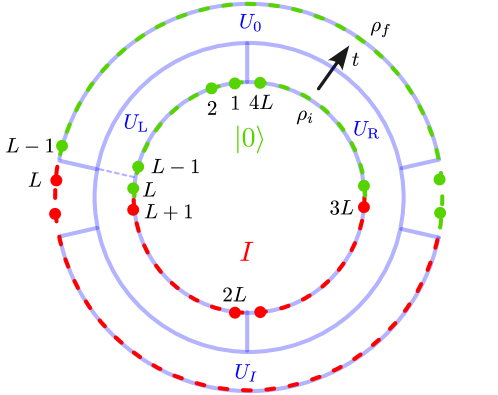
Figure 1: Sketch of the quantum circuit $\widetilde{U}=\left(U_{I}\otimes U_{0}\right)\cdot\left(U_{\rm L}\otimes U_{\rm R}\right)$ that cannot achieve the shift operator. In the initial state (24), the top half of the figure is $|0\rangle\langle 0|$ while the bottom half is $I$ on each site.

Proof.

To show (9), it suffices to find an approximation $\widetilde{U}$ of $U$ such that

$$\left\lVert U-\widetilde{U}\right\rVert \leq\frac{1}{8},$$ (16a)

$$\left\lVert\widetilde{U}-U_{\rm sh}\right\rVert \geq\frac{1}{4},$$ (16b)

because from the triangle inequality,

$$\left\lVert U-U_{\rm sh}\right\rVert\geq\left\lVert\widetilde{U}-U_{\rm sh}\right\rVert-\left\lVert U-\widetilde{U}\right\rVert\geq\frac{1}{4}-\frac{1}{8}=\frac{1}{8}.$$ (17)

We will choose $\widetilde{U}$ as a quantum circuit (of very large gate size!) that approximations the Hamiltonian evolution, using ideas from Osborne (2006); Haah et al. (2020). To this end, we first invoke the following Lemma to cut the coupling between site $0$ and $1$:

Lemma 2.3.

If (15) holds for constant

$$C=1+\log\frac{16c_{\rm LR}}{\mu v},$$ (18)

there exists a unitary $U_{0}$ acting on region $\{2-L,3-L,\cdots,L-1\}$, such that

$$\left\lVert U-U_{0}\cdot U_{\rm op}\right\rVert\leq\frac{1}{16},$$ (19)

where

$$U_{\rm op}=\mathcal{T}\mathrm{e}^{-\mathrm{i}\int^{T}_{0}\mathrm{d}t\left[H(t)-H_{01}(t)\right]},$$ (20)

is generated by $H$ with open boundary.

We will prove this Lemma in Section 2.2. We then similarly cut $U_{\rm op}$ between sites $2L,2L+1$:

$$\left\lVert U_{\rm op}-U_{I}\cdot(U_{\rm L}\otimes U_{\rm R})\right\rVert\leq\frac{1}{16},$$ (21)

where $U_{\rm L}$ ($U_{\rm R}$) is supported on the left (right) half chain $x=1,\cdots,2L$ ($x=2L+1,\cdots,4L$), and generated by the Hamiltonian terms inside the half chain. Analogous to $U_{0}$, $U_{I}$ is supported on sites $x=L+2,\cdots,3L-1$, where the meaning of subscripts $0,I$ will become clear later. To summarize, we choose

$$\widetilde{U}=\left(U_{I}\otimes U_{0}\right)\cdot\left(U_{\rm L}\otimes U_{\rm R}\right),$$ (22)

as shown by the four blue blocks in Fig. 1, and the following corollary holds by the triangle inequality from Lemma 2.3 and the analogous (21):

Corollary 2.4.

(18) leads to (16a).

To conclude the proof, it remains to show (16b). We focus on a particular initial state $\rho_{i}$, and show it is hard to prepare the target final state

$$\rho_{f}:=U_{\mathrm{sh}}\rho_{i}U_{\mathrm{sh}}^{\dagger},$$ (23)

using $\widetilde{U}$. The state $\rho_{i}$ is defined as follows. We choose identities on spin $L+1,\cdots,3L$, and $\ket{0}$ otherwise:

$$\rho_{i}=\bigotimes_{x=1-L}^{L}\ket{0}_{x}\bra{0}\otimes\bigotimes_{x=L+1}^{3L}\frac{I_{x}}{2},$$ (24)

so that

$$\rho_{f}=\bigotimes_{x=-L}^{L-1}\ket{0}_{x}\bra{0}\otimes\bigotimes_{x=L}^{3L-1}\frac{I_{x}}{2}.$$ (25)

As a result, $U_{I}$ acts inside the identity region, for either $\rho_{i}$ or $\rho_{f}$; similar for $U_{0}$, which justifies the subscripts. For these states, we prove the following Lemma in Section 2.3:

Lemma 2.5.

$\widetilde{U}$ does not efficiently implement shift:

$$\left\lVert\widetilde{U}\rho_{i}\widetilde{U}^{\dagger}-\rho_{f}\right\rVert_{1}\geq 1/2.$$ (26)

With these two lemmas in hand, (26) then leads to (16b) because

$$\left\lVert\widetilde{U}\rho_{i}\widetilde{U}^{\dagger}-U_{\mathrm{sh}}\rho_{i}U_{\mathrm{sh}}^{\dagger}\right\rVert_{1} =\left\lVert\left(\widetilde{U}-U_{\mathrm{sh}}\right)\rho_{i}\widetilde{U}^{\dagger}+U_{\mathrm{sh}}\rho_{i}\left(\widetilde{U}-U_{\mathrm{sh}}\right)^{\dagger}\right\rVert_{1}\leq\left\lVert\left(\widetilde{U}-U_{\mathrm{sh}}\right)\rho_{i}\widetilde{U}^{\dagger}\right\rVert_{1}+\left\lVert U_{\mathrm{sh}}\rho_{i}\left(\widetilde{U}-U_{\mathrm{sh}}\right)^{\dagger}\right\rVert_{1}$$

$$\leq\left\lVert\widetilde{U}-U_{\mathrm{sh}}\right\rVert+\left\lVert\widetilde{U}-U_{\mathrm{sh}}^{\dagger}\right\rVert=2\left\lVert\widetilde{U}-U_{\mathrm{sh}}\right\rVert.$$ (27)

We used triangle inequality in the first line, and Hölder’s inequality $\left\lVert AB\right\rVert_{1}\leq\left\lVert A\right\rVert\left\lVert B\right\rVert_{1}$ with $\left\lVert\rho_{i}\right\rVert_{1}=\left\lVert U\right\rVert=1$ in the second line. This concludes the proof: we have shown (16a), and how (9) follows from (16a) and (16b). ∎

2.2 Circuit approximation of Hamiltonian evolution

Proof of Lemma 2.3.

For notational simplicity we assume $H$ is time-independent in this proof, because the time-dependent case generalizes immediately. In the interaction picture,

$$UU_{\rm op}^{\dagger}=\mathrm{e}^{-\mathrm{i}TH}\mathrm{e}^{\mathrm{i}T(H-H_{01})}=\tilde{\mathcal{T}}\mathrm{e}^{-\mathrm{i}\int^{T}_{0}H_{01}(t)\mathrm{d}t},\quad\mathrm{where}\quad H_{01}(t):=\mathrm{e}^{-\mathrm{i}t(H-H_{01})}H_{01}\mathrm{e}^{\mathrm{i}t(H-H_{01})},$$ (28)

and $\tilde{\mathcal{T}}$ is anti-time ordering. This can be verified by taking time derivative.

$H_{01}(t)$ obeys Lieb-Robinson bound (14), so it is largely supported inside the region $S_{r}:=\{x:\mathsf{d}(x,\{0,1\})\leq r\}=\{2-L,\cdots,L-1\}$ with $r=L-2$ (namely, $S_{r}$ is the initial support $\{0,1\}$ expanded by distance $r$). More precisely, Theorem 2.1 implies (see e.g. Proposition 4.1 in Chen et al. (2023a)):

$$\left\lVert H_{01}(t)-\mathbb{P}_{r}H_{01}(t)\right\rVert\leq c_{\rm LR}\mathrm{e}^{\mu(vt-L+1)},$$ (29)

where we have used $\left\lVert H_{01}\right\rVert\leq 1$ from (13), and

$$\mathbb{P}_{r}H_{01}(t):=\int_{S_{r}^{\rm c}}\mathrm{d}VV^{\dagger}H_{01}(t)V$$ (30)

with $V$ being a Haar random unitary acting on the complement $S_{r}^{\rm c}$. $\mathbb{P}_{r}$ is a superoperator (linear transformation on the vector space of operators) that selects the part $\mathbb{P}_{r}H_{01}(t)$ whose support is contained inside $S_{r}$. Define

$$U_{0}:=\tilde{\mathcal{T}}\mathrm{e}^{-\mathrm{i}\int^{T}_{0}\mathrm{d}t\,\mathbb{P}_{r}H_{01}(t)},$$ (31)

supported in $S$. By the Duhamel identity,

$$\left\lVert UU_{\rm op}^{\dagger}-U_{0}\right\rVert =\left\lVert-\mathrm{i}\int^{T}_{0}\mathrm{d}t\tilde{\mathcal{T}}\mathrm{e}^{-\mathrm{i}\int^{t}_{0}H_{01}(t_{1})\mathrm{d}t_{1}}\left[H_{01}(t)-\mathbb{P}_{r}H_{01}(t)\right]\mathrm{e}^{-\mathrm{i}\int^{T}_{t}\mathbb{P}_{r}H_{01}(t_{2})\mathrm{d}t_{2}}\right\rVert$$

$$\leq\int^{T}_{0}\mathrm{d}t\left\lVert H_{01}(t)-\mathbb{P}_{r}H_{01}(t)\right\rVert\leq\frac{c_{\rm LR}}{\mu v}\mathrm{e}^{\mu(vT-L+1)},$$ (32)

where we have used (29). Because $\left\lVert U-U_{0}U_{\rm op}^{\dagger}\right\rVert=\left\lVert UU_{\rm op}^{\dagger}-U_{0}\right\rVert$, (19) holds by setting

$$\frac{c_{\rm LR}}{\mu v}\mathrm{e}^{\mu(vT-L+1)}\leq\frac{1}{16},$$ (33)

which is equivalent to (18). This lemma is, therefore, reminiscent of the HHKL algorithm Haah et al. (2020). ∎

2.3 The quantum circuit approximation does not shift the particular state

Proof of Lemma 2.5.

We manipulate the goal (26) as follows:

$$\frac{1}{2} \leq\left\lVert\widetilde{U}\rho_{i}\widetilde{U}^{\dagger}-\rho_{f}\right\rVert_{1}$$

$$=\left\lVert\left(U_{\rm L}\otimes U_{\rm R}\right)\rho_{i}\left(U_{\rm L}\otimes U_{\rm R}\right)^{\dagger}-\left(U_{\rm I}\otimes U_{\rm 0}\right)^{\dagger}\rho_{f}\left(U_{\rm I}\otimes U_{\rm 0}\right)\right\rVert_{1}$$

$$=\left\lVert\left(U_{\rm L}\otimes U_{\rm R}\right)\rho_{i}\left(U_{\rm L}\otimes U_{\rm R}\right)^{\dagger}-U_{\rm 0}^{\dagger}\rho_{f}U_{\rm 0}\right\rVert_{1}.$$ (34)

In the second line we have used $\left\lVert VOV^{\dagger}\right\rVert_{1}=\left\lVert O\right\rVert_{1}$ for any unitary $V$. In the last line we used the fact that $U_{I}$ acts trivially on the identity region in $\rho_{f}$. Taking partial trace in the last line of (34) and using monotonicity of trace distance: $\left\lVert\mathrm{tr}_{\rm R}(\rho-\rho^{\prime})\right\rVert_{1}\leq\left\lVert\rho-\rho^{\prime}\right\rVert_{1}$, it then suffices to show

$$\frac{1}{2}\leq\left\lVert U_{\rm L}\rho_{i,\rm L}U_{\rm L}^{\dagger}-\mathrm{tr}_{\rm R}\left(U_{\rm 0}^{\dagger}\rho_{f}U_{\rm 0}\right)\right\rVert_{1}.$$ (35)

$\rho_{i,\rm L}$ is the restriction of $\rho_{i}$ in the left half chain that contains $L$ identities, so the density matrix has $2^{L}$ nonzero eigenvalues (Schmidt values) that are all equal to $2^{-L}$. In other word, there is a basis $\{\ket{j}:j=1,\cdots,2^{2L}\}$ such that

$$U_{\rm L}\rho_{i,\rm L}U_{\rm L}^{\dagger}=2^{-L}\begin{pmatrix}I&0\\ 0&0\end{pmatrix},$$ (36)

where each block is $2^{L}\times 2^{L}$. On the other hand, $\rho_{f}$ has $L+1$ identities in the left half chain, and $U_{0}$ acts on an all-zero region of $\rho_{f}$ (across the left and right half chain). As a result

$$\left\lVert\mathrm{tr}_{\rm R}\left(U_{\rm 0}^{\dagger}\rho_{f}U_{\rm 0}\right)\right\rVert=2^{-L-1}\left\lVert I\otimes\mathrm{tr}_{\rm R}\left(U_{\rm 0}^{\dagger}\ket{0}\bra{0}U_{\rm 0}\right)\right\rVert\leq 2^{-L-1},$$ (37)

because the operator inside the norm is a density matrix $\rho$ with $\left\lVert\rho\right\rVert\leq 1$. In words, this holds because in region R $\rho_{f}$ already is a mixed state with $L+1$ bits, and the unitary $U_{0}$ can only further increase the entanglement between R and L as it acts only on the sites where $\rho_{f}$ is pure.

Such spectral difference leads to large $1$-norm of operator $O:=U_{\rm L}\rho_{i,\rm L}U_{\rm L}^{\dagger}-\mathrm{tr}_{\rm R}\left(U_{\rm 0}^{\dagger}\rho_{f}U_{\rm 0}\right)$, because

$$\left\lVert O\right\rVert_{1} =\max_{V}\left|\mathrm{tr}OV\right|\geq\sum_{j}\left|O_{jj}\right|\geq\sum_{j\leq 2^{L}}O_{jj}$$

$$=\sum_{j\leq 2^{L}}2^{-L}-\left[\mathrm{tr}_{\rm R}\left(U_{\rm 0}^{\dagger}\rho_{f}U_{\rm 0}\right)\right]_{jj}$$

$$\geq\sum_{j\leq 2^{L}}(2^{-L}-2^{-L-1})=\frac{1}{2}.$$ (38)

Here in the first inequality, we have chosen the particular unitary $V$ that is diagonal in the basis (36), with the $j$-th diagonal element $V_{jj}=\mathrm{sign}(O_{jj})$. In the second line, we have used (36) in this basis. The last line comes from $\left[\mathrm{tr}_{\rm R}\left(U_{\rm 0}^{\dagger}\rho_{f}U_{\rm 0}\right)\right]_{jj}\leq\left\lVert\mathrm{tr}_{\rm R}\left(U_{\rm 0}^{\dagger}\rho_{f}U_{\rm 0}\right)\right\rVert$ and (37). This proves (35), which then leads to (26). ∎

2.4 Long-range interactions

Having gained the key intuition for why the shift is hard to implement using local interactions, we now turn to our main goal, namely the study of implementing shift using power-law interactions. In what follows, we assume (8) and fix units of time by setting $K=1$.

To proceed, we will need the following Lieb-Robinson bound:

Theorem 2.6.

Kuwahara and Saito (2020); Tran et al. (2021a); Chen et al. (2023a) Assuming (8), there exists constants $c_{\rm LR},v,\epsilon>0$ where $\epsilon$ can be arbitrarily small, such that for any local operator $A$,

$$\left\lVert A(t)-\mathbb{P}_{r}A(t)\right\rVert\leq\left\lVert A\right\rVert g_{\alpha}(t,r)$$ (39)

where

$$g_{\alpha}(t,r):=c_{\rm LR}\cdot\left\{\begin{array}[]{ccc}t^{2}(r-vt)^{1-\alpha}&(t\leq r/v),&\alpha>3\\ \left(\frac{t}{r^{\alpha-2-\epsilon}}\right)^{\frac{\alpha-1}{\alpha-2}-\frac{\epsilon}{2}}&(t\leq r^{\alpha-2-\epsilon}/v),&2<\alpha\leq 3\end{array}\right..$$ (40)

Here $\mathbb{P}_{r}A(t)$ is supported only on sites of distance $\leq r$ to the initial local operator $A$.

Proof.

(39) is contained in the literature except for the point $\alpha=3$, which we focus on here. For any $\epsilon\in(0,1)$, a system with $\alpha=3$ also satisfies (8) with exponent $\alpha^{\prime}:=3-\epsilon/2\in(2,3)$. Then one can use (39) with $\alpha$ set to $\alpha^{\prime}$ and $\epsilon$ set to $\epsilon^{\prime}:=\epsilon/2$, so that

$$\left\lVert A(t)-\mathbb{P}_{r}A(t)\right\rVert \leq c_{\rm LR}\left\lVert A\right\rVert\left(\frac{t}{r^{\alpha^{\prime}-2-\epsilon^{\prime}}}\right)^{\frac{\alpha^{\prime}-1}{\alpha^{\prime}-2}-\frac{\epsilon^{\prime}}{2}}=c_{\rm LR}\left\lVert A\right\rVert\left(\frac{t}{r^{\alpha-2-\epsilon}}\right)^{\frac{\alpha^{\prime}-1}{\alpha^{\prime}-2}-\frac{\epsilon^{\prime}}{2}}=c_{\rm LR}^{\prime}\left\lVert A\right\rVert\left(\frac{vt}{r^{\alpha-2-\epsilon}}\right)^{\frac{\alpha^{\prime}-1}{\alpha^{\prime}-2}-\frac{\epsilon^{\prime}}{2}}$$

$$\leq c_{\rm LR}^{\prime}\left\lVert A\right\rVert\left(\frac{vt}{r^{\alpha-2-\epsilon}}\right)^{\frac{\alpha-1}{\alpha-2}-\frac{\epsilon}{2}},\quad\mathrm{for}\quad t\leq r^{\alpha^{\prime}-2-\epsilon^{\prime}}/v=r^{\alpha-2-\epsilon}/v.$$ (41)

Here $c_{\rm LR}^{\prime}=c_{\rm LR}v^{-\frac{\alpha^{\prime}-1}{\alpha^{\prime}-2}+\frac{\epsilon^{\prime}}{2}}$ in the first line, and we have used the base $vt/r^{\alpha-2-\epsilon}\leq 1$ and $\frac{\alpha^{\prime}-1}{\alpha^{\prime}-2}\geq\frac{\alpha-1}{\alpha-2}$ in the second line. (2.4) then becomes (39) at $\alpha=3$ by redefining the constant $c^{\prime}_{\rm LR}v^{\frac{\alpha-1}{\alpha-2}-\frac{\epsilon}{2}}\rightarrow c_{\rm LR}$. ∎

Theorem 2.2 can now be generalized to power law interactions:

Theorem 2.7.

For power-law interaction (8), if $L\geq L_{0}$ for some constant $L_{0}$, and the evolution time $T$ satisfies

$$vT\leq\left\{\begin{array}[]{cc}L-C,&\alpha\geq 4\\ CL^{\frac{\alpha-1}{3}},&3<\alpha<4\\ CL^{\frac{[\alpha-1-\epsilon(\alpha/2-1)](\alpha-2-\epsilon)}{2\alpha-3-\epsilon(\alpha/2-1)}},&2<\alpha\leq 3\end{array}\right.$$ (42)

for any $\epsilon>0$, and constant $0<C<\infty$ that may depend on $\epsilon$, then (9) holds: namely, $U$ is far from $U_{\mathrm{sh}}$.

Proof.

Following the proof of Theorem 2.2, we construct a circuit approximation $\widetilde{U}$ still of the form (22), as shown by the four blue blocks in Fig. 1. (16b) continues to hold because it only depends on the geometry of the circuit $\widetilde{U}$. Therefore, due to (17), we only need to prove $\widetilde{U}$ is a good approximation for $U$, i.e. (16a), in time window (42).

We follow Tran et al. (2019), which generalizes Haah et al. (2020) to “circuitize” power-law Hamiltonian dynamics. The complication is that when cutting the chain open between site $0$ and $1$, there are many couplings $H_{xy}$ to deal with instead of just one $H_{01}$ in the local case. We separate the couplings into two groups.

The first group of couplings are highly long-range ones that we can ignore directly. More precisely, we ignore Hamiltonian terms

$$H_{\rm far}=\sum_{\begin{subarray}{c}1\leq x\leq 2L,2L<y\leq N:\\ \mathsf{d}(x,y)\geq\ell\end{subarray}}H_{xy},$$ (43)

that couple the left and right half-chain and act on spins of distance $\geq\ell$. The remaining Hamiltonian terms generate $U_{-\rm far}:=\tilde{\mathcal{T}}\mathrm{e}^{-\mathrm{i}\int^{T}_{0}\mathrm{d}t\left[H(t)-H_{\rm far}(t)\right]}$. To choose $\ell$, we bound the error in a similar way as (2.2):

$$\left\lVert U-U_{-\rm far}\right\rVert \leq T\left\lVert H_{\rm far}\right\rVert\leq T\sum_{\begin{subarray}{c}1\leq x\leq 2L,2L<y\leq N:\\ \mathsf{d}(x,y)\geq\ell\end{subarray}}\left\lVert H_{xy}\right\rVert$$

$$\leq 2T\sum_{x>0,y<0:x-y\geq\ell}(x-y)^{-\alpha}=2T\sum_{r\geq\ell}r\cdot r^{-\alpha}\leq c_{\alpha}T\ell^{2-\alpha},$$ (44)

for a constant $c_{\alpha}$ if $\alpha>2$. To get the second line, we have used (8) and relaxed the sum to $2$ cuts each for an infinite chain. We therefore choose

$$\ell:=(16c_{\alpha}T)^{1/(\alpha-2)},$$ (45)

such that

$$\left\lVert U-U_{-\rm far}\right\rVert\leq\frac{1}{16}.$$ (46)

Moreover, assuming (42), one can verify that $\ell\lesssim L^{\beta}$ for some $\beta<1$, for all $\alpha$ regimes considered. Therefore, at sufficiently large $L\geq L_{0}$, (42) implies

$$\ell\leq 0.1L.$$ (47)

In other words, one can always ignore the longest-scale $\sim L$ couplings.

Due to (46) and triangle inequality, it remains to prove

$$\left\lVert U_{-\rm far}-\widetilde{U}\right\rVert\leq\frac{1}{16}.$$ (48)

Since there are two cuts between left and right, we focus on one cut to show

$$\left\lVert U_{-\rm far}-U_{0}U_{\rm op}\right\rVert\leq\frac{1}{32},$$ (49)

where $U_{\rm op}$ is generated by open-boundary Hamiltonian $H-H_{\rm far}-H_{\rm cut}$ with

$$H_{\rm cut}:=\sum_{\begin{subarray}{c}x<0,y>0:\\ y-x<\ell\end{subarray}}H_{xy}.$$ (50)

Following the proof of Lemma 2.3 where $H$ is assumed time-independent for simplicity,

$$\left\lVert U_{-\rm far}-U_{0}U_{\rm op}\right\rVert \leq T\max_{t}\left\lVert H_{\rm cut}(t)-\mathbb{P}_{S}H_{\rm cut}(t)\right\rVert\leq T\max_{t}\sum_{\begin{subarray}{c}x<0,y>0:\\ y-x<\ell\end{subarray}}\left\lVert H_{xy}(t)-\mathbb{P}_{S}H_{xy}(t)\right\rVert$$

$$\leq T\sum_{\begin{subarray}{c}x<0,y>0:\\ y-x<\ell\end{subarray}}(y-x)^{-\alpha}g(T,0.9L)\leq c_{\alpha}^{\prime}Tg(T,0.9L),$$ (51)

for some constant $c_{\alpha}^{\prime}$ because the sum over $x,y$ converges for $\alpha>2$. Here in the first line, $\mathbb{P}_{S}H_{\rm cut}(t)$ is the part of $H_{\rm cut}(t)$ acting inside $S=\{2-L,\cdots,L-1\}$. The second line comes from (39), (8) and that the distance from any $H_{xy}$ included to the outside of $S$ is larger than $L-\ell\geq 0.9L$ from (47). We then demand $c^{\prime}_{\alpha}Tg_{\alpha}(T,0.9L)\leq 1/32$, which for $\alpha\in(2,3]$ becomes

$$T^{1+\frac{1}{\frac{\alpha-1}{\alpha-2}-\frac{\epsilon}{2}}}\leq C^{\prime}L^{\alpha-2-\epsilon},$$ (52)

for some constant $C^{\prime}$, which reduces to the third line of (42) for some constant $C$. The first two lines work similarly, because for $3<\alpha$, the error is large so long as $T^{3}/(L-vT)^{\alpha-1}$ is small.

To summarize, (42) guarantees (49), which implies (48) by treating the other cut similarly, and further (16a) by combining (46). Finally, this yields (9) following the proof of Lemma 2.3. ∎

The bound (42) is probably not qualitatively tight for realizing the shift unitary at $\alpha<4$, since we only compared the unitary action on a particular state $\rho_{i}$. In the next section, we will present tighter bounds than (42) at sufficiently small $\alpha$. Conceptually, the previous proof argues that entanglement (or, purity) stored in identities cannot be transported easily, and it is conjectured in Chen and Lucas (2021) that entanglement is governed by Frobenius light cone for power law interactions, which cares about all states; this conjecture is compatible with Gong et al. (2017).

For the specific task of mapping $\rho_{i}$ to $\rho_{f}$, i.e. transferring an identity local density matrix, it can be achieved by state-transfer protocols $U$:

$$U(\alpha\ket{0}_{x}+\beta\ket{1}_{x})\otimes\ket{\bm{0}}_{x+1,\cdots,y}=\ket{\bm{0}}_{x,\cdots,y-1}\otimes(\alpha\ket{0}_{y}+\beta\ket{1}_{y}),$$ (53)

that transfers a qubit information from $x=-L$ to $y=L$ in a background of $0$s. Such protocols have been constructed Tran et al. (2021b) that asymptotically matches the Lieb-Robinson bound (39); however, these protocols do not saturate (42) because of the extra $T$ factor in (2.4). As stated in the introduction, we conjecture that our bounds are not optimal.

3 Frobenius perspective

As we now show, Theorem 2.7 is not optimal at small $\alpha$. To show this result, we will need to take a rather different perspective, based on the Frobenius light cone Chen and Lucas (2021). Intuitively, Frobenius bounds study the Frobenius norm, which we define as

$$\lVert A\rVert_{\mathrm{F}}=\sqrt{\frac{\mathrm{tr}(A^{\dagger}A)}{\mathrm{tr}(1)}}.$$ (54)

This object may be interpreted more physically as bounding the size of typical matrix elements of $A$, rather than the largest matrix element of $A$ possible (the latter is the definition of the operator norm $\lVert A\rVert$). If we can successfully implement $U_{\mathrm{sh}}$, we must implement it in a typical state, so it is natural to expect that the time needed to implement a shift operator can be bounded by studying Frobenius light cones.

3.1 Operator growth formalism

We now introduce a useful notation for developing these Frobenius bounds. The key is to view operator growth as a quantum walk in the Hilbert space of operators. An operator basis for the operator space is Pauli strings, with local basis on each site being the four Pauli matrices denoted by $\{\left|I\right),\left|X\right),\left|Y\right),\left|Z\right)\}$. Inner product between operators and the induced Frobenius norm are defined by

$$\left(O|O^{\prime}\right):=2^{-N}\mathrm{tr}(O^{\dagger}O^{\prime}),$$ (55)

where the normalization ensures that each Pauli string has norm $1$. Notice that $\left\lVert O\right\rVert_{\rm F}=\sqrt{\left(O|O\right)}$. For comparison, in this section we denote the usual operator norm as $\left\lVert O\right\rVert_{\infty}\geq\left\lVert O\right\rVert_{\rm F}$.

Superoperators are defined as linear maps acting within this operator Hilbert space. We have already encountered the superprojector $\mathbb{P}$ in (30). In addition, we will use the super-identity on a site

$$\mathcal{I}=\left|I\right)\left(I\right|+\left|X\right)\left(X\right|+\left|Y\right)\left(Y\right|+\left|Z\right)\left(Z\right|,$$ (56)

which makes $\mathcal{I}/4$ into a super-density-matrix. The evolution superoperators

$$\mathcal{U}\left|O\right)=\left|U^{\dagger}OU\right),\quad\mathcal{U}_{\rm sh}\left|O\right)=\left|U_{\rm sh}^{\dagger}OU_{\rm sh}\right),$$ (57)

are still unitary because $\left(O\right|\mathcal{U}^{\dagger}\mathcal{U}\left|O\right)=2^{-N}\mathrm{tr}\left[(U^{\dagger}OU)^{\dagger}U^{\dagger}OU\right]=\left(O|O\right)$. The distance between two superunitaries $\mathcal{U},\mathcal{V}$ can be quantified by e.g. $\infty$-norm induced by the operator Frobenius norm:

$$\left\lVert\mathcal{U}-\mathcal{V}\right\rVert_{\infty,\mathrm{F}}:=\max_{O:\left\lVert O\right\rVert_{\rm F}=1}\left\lVert(\mathcal{U}-\mathcal{V})\left|O\right)\right\rVert_{\rm F}.$$ (58)

As its dual, the trace distance between two super-density-matrices $\mathcal{R},\mathcal{R}^{\prime}$ is

$$\left\lVert\mathcal{R}-\mathcal{R}^{\prime}\right\rVert_{1,\mathrm{F}}:=\max_{\mathcal{O}:\left\lVert\mathcal{O}\right\rVert_{\infty,\mathrm{F}}=1}\mathrm{Tr}[\mathcal{O}(\mathcal{R}-\mathcal{R}^{\prime})],$$ (59)

where $\mathrm{Tr}$ is the super-trace in operator space.

The evolution

$$\mathcal{U}=\mathrm{e}^{\int^{T}_{0}\mathrm{d}t\,\mathcal{L}(t)}$$ (60)

is generated by Liouvillian $\mathcal{L}(t)=\sum_{a}\mathcal{L}_{a}(t)$ where

$$\mathcal{L}_{a}(t)\left|O\right):=\mathrm{i}\left|[H_{a}(t),O]\right),$$ (61)

with $H_{a}$ being the local terms of $H$.

3.2 Frobenius bound on realizing shift with long-range interactions

For power-law interaction (8), now we further assume $K=1$ and

$$\mathrm{tr}[H_{xy}(t)]=0,$$ (62)

which is satisfied easily by subtracting an identity operator for each term. There is a Frobenius light cone that can be asymptotically slower than Lieb-Robinson (i.e. the light cone for $\infty$-norm bound):

Theorem 3.1.

Chen and Lucas (2021) Given (8), there exists constants $c_{\rm FB}$ determined by $\alpha$, such that for any local operator $A$,

$$\left\lVert A(t)-\mathbb{P}_{r}A(t)\right\rVert_{\rm F}\leq\left\lVert A\right\rVert_{F}f_{\alpha}(t,r)$$ (63)

where

$$f_{\alpha}(t,r):=c_{\rm FB}\,t\cdot\left\{\begin{array}[]{cc}\log(r)/r,&\alpha>2\\ \log^{2}(r)/r,&\alpha=2\\ r^{1-\alpha},&1<\alpha<2\end{array}\right.$$ (64)

Using this result, we can improve Theorem 2.7 to:

Theorem 3.2.

For power-law interaction (8), if $L\geq L_{0}$ for some constant $L_{0}$, and the evolution time $T$ satisfies

$$T\leq C_{\rm FB}\cdot\left\{\begin{array}[]{cc}\sqrt{L/\log L},&\alpha>2\\ \sqrt{L/\log^{2}L},&\alpha=2\\ L^{(\alpha-1)/2},&1<\alpha<2\end{array}\right.$$ (65)

for some constant $C_{\rm FB}$, then

$$\left\lVert U-U_{\rm sh}\right\rVert_{\rm F}\geq 1/8,$$ (66)

so that $U$ does not realize shift operation.

Before the proof, let us compare Theorems 3.2 and 2.7. The distance metric is stronger here because $\left\lVert U-U_{\rm sh}\right\rVert_{\rm F}\leq\left\lVert U-U_{\rm sh}\right\rVert$; namely, in the time window (65), $U$ does not perform shift for a typical state. Comparing the time window, the previous upper bound (42) is parametrically larger (stronger) for sufficiently large $\alpha$, and vice versa for small $\alpha$. In particular, there is an exponential separation at $\alpha\in(0,1)$, where $T$ is algebraic with $L$ in (65), while (42) would become $T=\mathrm{O}(\mathrm{polylog}(L))$ if using the Lieb-Robinson bound $g_{\alpha}(t,r)\sim\mathrm{e}^{\mu t}r^{-\alpha}$ Hastings and Koma (2006) in this $\alpha$ regime. The critical $\alpha_{\rm c}\in(2,3)$ where (65) and (42) coincide is

$$\frac{[\alpha-1-\epsilon(\alpha/2-1)](\alpha-2-\epsilon)}{2\alpha-3-\epsilon(\alpha/2-1)}=\frac{1}{2}-\epsilon^{\prime},\quad\Rightarrow\quad\alpha\approx\alpha_{\rm c}=2+1/\sqrt{2},$$ (67)

where we have set $\epsilon,\epsilon^{\prime}\rightarrow 0$. The Frobenius bound Theorem 3.2 is then stronger for $\alpha<\alpha_{\rm c}$; for $\alpha>\alpha_{\rm c}$, the two Theorems are in general not comparable because the metric is different.

Proof.

The proof mimics that of Theorem 2.2 and 2.7, where we basically replace all $\left\lVert V-V^{\prime}\right\rVert$ with Frobenius norm $\left\lVert V-V^{\prime}\right\rVert_{\rm F}$. This is valid because one still has triangle inequality for Frobenius norm

$$\left\lVert A-B\right\rVert_{\rm F}\leq\left\lVert A\right\rVert_{\rm F}+\left\lVert B\right\rVert_{\rm F}.$$ (68)

As one can verify, we only need to prove the following three inequalities.

$$\left\lVert U-U_{-\rm far}\right\rVert_{\rm F} \leq 1/16,$$ (69a)

$$\left\lVert U_{-\rm far}-\widetilde{U}\right\rVert_{\rm F} \leq 1/16,$$ (69b)

$$\left\lVert\widetilde{U}-U_{\rm sh}\right\rVert_{\rm F} \geq 1/4.$$ (69c)

Here $U_{-\rm far}$ is generated by $H-H_{\rm far}$ with $H_{\rm far}$ defined in (43) where the parameter $\ell$ is determined shortly.

We proceed one by one. For (69a), similar to (2.4) we have

$$\left\lVert U-U_{-\rm far}\right\rVert_{\rm F} \leq T\left\lVert H_{\rm far}\right\rVert_{\rm F}$$

$$\leq T\sqrt{\sum_{\begin{subarray}{c}1\leq x\leq 2L,2L<y\leq N:\\ \mathsf{d}(x,y)\geq\ell\end{subarray}}\left\lVert H_{xy}\right\rVert_{\rm F}^{2}}$$

$$\leq 2T\sqrt{\sum_{x>0,y<0:x-y\geq\ell}(x-y)^{-2\alpha}}=2T\sqrt{\sum_{r\geq\ell}r\cdot r^{-2\alpha}}\leq\tilde{c}_{\alpha}T\ell^{1-\alpha},$$ (70)

for some constant $\tilde{c}_{\alpha}$ if $\alpha>1$. Here the second line comes from orthogonality $\left(H_{xy}|H_{x^{\prime}y^{\prime}}\right)=0$ if $(x,y)\neq(x^{\prime},y^{\prime})$ due to (62). To get the third line, we used $\left\lVert H_{xy}\right\rVert_{\rm F}\leq\left\lVert H_{xy}\right\rVert$. We therefore choose

$$\ell:=(16c_{\alpha}T)^{1/(\alpha-1)},$$ (71)

such that (69a) holds. Moreover, one can verify that (65) implies $\ell\leq 0.1L$ (47) for sufficiently large $L\geq L_{0}$.

(69b) just comes from (2.4) with $\infty$-norms changed to Frobenius norm, $g_{\alpha}(t,r)$ substituted by $f_{\alpha}(t,r)$, and direct computation of $Tf_{\alpha}(T,0.9L)=\mathrm{O}(1)$.

For (69c), observe that in the proof of Lemma 2.5, we only demand the $S:=\{1-L,\cdots,L\}$ subsystem in $\rho_{i}$ to be a pure direct product state (see arguments around (36) and (37)). Therefore Lemma 2.5 actually proves that

$$\left\lVert\widetilde{U}\rho_{i}(z)\widetilde{U}^{\dagger}-\rho_{f}(z)\right\rVert_{1}\geq\frac{1}{2},$$ (72)

for any string $z\in\{0,1\}^{2L}$, where

$$\rho_{i}(z):=\bigotimes_{x=1-L}^{L}\ket{z_{x}}_{x}\bra{z_{x}}\otimes\bigotimes_{x=L+1}^{3L}\frac{I_{x}}{2},$$ (73)

(so that the previous $\rho_{i}=\rho_{i}(0\cdots 0)$), and $\rho_{f}(z):=U_{\rm sh}\rho_{i}(z)U_{\rm sh}^{\dagger}$. We need to relate (72) to (69c).

For each $z$ string, one can purify the system by a $2^{2L}$-dimensional ancilla (labeled by $\rm A$) so that

$$\rho_{i}(z)=\mathrm{tr}_{\rm A}\ket{\Psi_{i}(z)}\bra{\Psi_{i}(z)}.$$ (74)

(72) then bounds the fidelity between pure states $\widetilde{U}\ket{\Psi_{i}(z)}$ and $\ket{\Psi_{f}(z)}:=U_{\rm sh}\ket{\Psi_{i}(z)}$ (here $\widetilde{U}$, for example, is shorthand notation for $\widetilde{U}\otimes I_{\rm A}$ acting on the enlarged Hilbert space)

$$2\left(1-\left|\bra{\Psi_{i}(z)}U_{\rm sh}^{\dagger}\widetilde{U}\ket{\Psi_{i}(z)}\right|\right) \geq 1-\left|\bra{\Psi_{i}(z)}U_{\rm sh}^{\dagger}\widetilde{U}\ket{\Psi_{i}(z)}\right|^{2}$$

$$=\frac{1}{4}\left\lVert\widetilde{U}\ket{\Psi_{i}(z)}\bra{\Psi_{i}(z)}\widetilde{U}^{\dagger}-U_{\rm sh}\ket{\Psi_{i}(z)}\bra{\Psi_{i}(z)}U_{\rm sh}^{\dagger}\right\rVert_{1}^{2}$$

$$\geq\frac{1}{4}\left\lVert\widetilde{U}\rho_{i}(z)\widetilde{U}^{\dagger}-\rho_{f}(z)\right\rVert_{1}^{2}\geq\frac{1}{16}.$$ (75)

Here the first line comes from $1+\left|\bra{\Psi_{i}(z)}U_{\rm sh}^{\dagger}\widetilde{U}\ket{\Psi_{i}(z)}\right|\leq 2$, the second line comes from the relation between fidelity and trace-norm for pure states, and the last line comes from monotonicity under partial trace over ancilla, together with (72).

On the other hand, the target

$$\left\lVert\widetilde{U}-U_{\rm sh}\right\rVert_{\rm F}^{2} =\left\lVert\widetilde{U}\right\rVert_{\rm F}^{2}+\left\lVert U_{\rm sh}\right\rVert_{\rm F}^{2}-\left[(U_{\rm sh}|\widetilde{U})+{\rm c.c.}\right]=2-2^{-4L}\left[\mathrm{tr}\left(U_{\rm sh}^{\dagger}\widetilde{U}\right)+{\rm c.c.}\right]$$

$$=2-2^{-4L}\left[\sum_{z}\mathrm{tr}\left((I_{S^{\rm c}}\otimes\ket{z}_{S}\bra{z})U_{\rm sh}^{\dagger}\widetilde{U}\right)+{\rm c.c.}\right]$$

$$\geq 2\cdot 2^{-2L}\sum_{z}1-\left|2^{-2L}\mathrm{tr}\left((I_{S^{\rm c}}\otimes\ket{z}_{S}\bra{z})U_{\rm sh}^{\dagger}\widetilde{U}\right)\right|$$

$$=2\cdot 2^{-2L}\sum_{z}1-\left|\bra{\Psi_{i}(z)}U_{\rm sh}^{\dagger}\widetilde{U}\ket{\Psi_{i}(z)}\right|\geq 2\cdot\frac{1}{32}=\frac{1}{16}.$$ (76)

Here all traces work in the physical system without the ancilla. We have used $\left\lVert V\right\rVert_{\rm F}=1$ for any unitary $V$ in the first line of (3.2), and inserted $I=I_{S^{\rm c}}\otimes\sum_{z}\ket{z}_{S}\bra{z}$ in the second line, where $S^{\rm c}=\{L+1,\cdots,3L\}$ is the complement of $S$. To get the last line, observe that when computing the fidelity in the enlarged Hilbert space, one can first trace over ancilla because $U_{\rm sh}^{\dagger}\widetilde{U}$ does not act on it, which leaves density matrix $2^{-2L}I_{S^{\rm c}}$ in $S^{\rm c}$ that exactly matches the third line. (3.2) is just (69c) by taking square root; the inequality is simply (75).

To summarize, we have proven all inequalities in (69), and plugging them into the proof of Theorem 2.7 establishes (66) by considering Frobenius norms throughout. ∎

3.3 The Super2 formalism: an alternate proof

Here we present an alternative proof that shift cannot be realized in time (42). The idea is to more seriously promote from the state Hilbert space to the operator space, as described in Section 3.1. Note that similar ideas also appear in bounding Frobenius light cones Chen and Lucas (2021), and quantifying information scrambling Zanardi (2022, 2023). For example, the super-density-matrices defined later in (82) correspond to subalgebras to be scrambled in Zanardi (2022).

Theorem 3.3.

Given the same conditions in Theorem 3.2, the superunitaries are far: There exists an operator $O$ with

$$\left\lVert O\right\rVert_{\infty}=1,$$ (77)

such that

$$\left\lVert\left(\mathcal{U}-\mathcal{U}_{\rm sh}\right)\left|O\right)\right\rVert_{{\rm F}}\geq\frac{1}{8}.$$ (78)

Therefore, $U$ does not realize the shift operation.

Theorem 3.3 implies 3.2 with a weaker constant $1/8\rightarrow 1/16$ in (66), because

$$\left\lVert\left(\mathcal{U}-\mathcal{U}_{\rm sh}\right)\left|O\right)\right\rVert_{{\rm F}} =\left\lVert U^{\dagger}OU-U_{\rm sh}^{\dagger}OU_{\rm sh}\right\rVert_{\rm F}\leq\left\lVert U^{\dagger}O\left(U-U_{\rm sh}\right)\right\rVert_{\rm F}+\left\lVert\left(U^{\dagger}-U_{\rm sh}^{\dagger}\right)OU_{\rm sh}\right\rVert_{\rm F}$$

$$\leq\left\lVert U^{\dagger}\right\rVert_{\infty}\left\lVert O\right\rVert_{\infty}\left\lVert U-U_{\rm sh}\right\rVert_{\rm F}+\left\lVert U^{\dagger}-U_{\rm sh}^{\dagger}\right\rVert_{\rm F}\left\lVert O\right\rVert_{\infty}\left\lVert U_{\rm sh}\right\rVert_{\infty}=2\left\lVert U-U_{\rm sh}\right\rVert_{\rm F},$$ (79)

where we have used triangle inequality in the first line, and Hölder’s inequality $\left\lVert AB\right\rVert_{\rm F}\leq\left\lVert A\right\rVert_{\infty}\left\lVert B\right\rVert_{\rm F}$ in the second line. (78) also implies the more compact version $\left\lVert\mathcal{U}-\mathcal{U}_{\rm sh}\right\rVert_{\infty,{\rm F}}\geq 1/8$ from $\left\lVert O\right\rVert_{\rm F}\leq\left\lVert O\right\rVert_{\infty}$ and the definition (58).

Proof.

The idea is to promote the proof of Theorem 2.2 from state (density matrix) space to operator (super-density-matrix) space, since the shift $U_{\rm sh}$ is also the super-shift $\mathcal{U}_{\rm sh}$. We call this approach the Super2 picture. The benefit is that some steps in the proof of Theorem 2.2 (e.g. Lemma 2.5) generalizes trivially after promotion, while now we can use the slower Frobenius light cone (63) as in Theorem 3.2.

Since triangle inequality still holds for the function $\left\lVert\cdot\left|O\right)\right\rVert_{\mathrm{F}}$ of superoperators, to prove (78) it suffices to show the analog of (69):

$$\left\lVert\left(\mathcal{U}-\mathcal{U}_{-\rm far}\right)\left|O\right)\right\rVert_{\rm F} \leq 1/16,$$ (80a)

$$\left\lVert\left(\mathcal{U}_{-\rm far}-\widetilde{\mathcal{U}}\right)\left|O\right)\right\rVert_{\rm F} \leq 1/16,$$ (80b)

$$\left\lVert\left(\widetilde{\mathcal{U}}-\mathcal{U}_{\rm sh}\right)\left|O\right)\right\rVert_{\rm F} \geq 1/4,$$ (80c)

for the to-be-determined operator $O$. Here $\mathcal{U}_{-\rm far},\widetilde{\mathcal{U}}$ are the superoperator versions of $U_{-\rm far},\widetilde{U}$ constructed in the proof of Theorem 3.2. In particular, $\widetilde{\mathcal{U}}$ has the circuit geometry in Fig. 1.

We first prove (80a) and (80b) for any $O$ normalized by (77). Similar to (3.3), we have

$$\left\lVert\left(\mathcal{U}-\mathcal{U}_{-\rm far}\right)\left|O\right)\right\rVert_{\rm F}\leq 2\left\lVert U-U_{-\rm far}\right\rVert_{\rm F}.$$ (81)

Following the proof of (69a), one has $\left\lVert U-U_{-\rm far}\right\rVert_{\rm F}\leq 1/32$ with a slightly different constant $1/16\rightarrow 1/32$ in (71), thus (81) implies (80a). (80b) follows similarly from adjusting the constant $1/16\rightarrow 1/32$ in (69b).

It remains to find an operator $O$ with (77) that satisfies (80c). Analogous to (24) and (25), we introduce super-density-matrices

$$\mathcal{R}_{i}:=\bigotimes_{x=1-L}^{L}\left|I\right)_{x}\left(I\right|\otimes\bigotimes_{x=L+1}^{3L}\frac{\mathcal{I}_{x}}{4},$$ (82)

so that

$$\mathcal{R}_{f}:=\mathcal{U}_{\rm sh}\mathcal{R}_{i}\mathcal{U}_{\rm sh}^{\dagger}=\bigotimes_{x=-L}^{L-1}\left|I\right)_{x}\left(I\right|\otimes\bigotimes_{x=L}^{3L-1}\frac{\mathcal{I}_{x}}{4}.$$ (83)

The super-identity region is frozen in dynamics, as we used previously; now the other $\left|I\right)$ region is also frozen from (88). Nevertheless, we do not need this extra observation: Lemma 2.5 generalizes verbatim to

$$\left\lVert\widetilde{\mathcal{U}}\mathcal{R}_{i}\widetilde{\mathcal{U}}^{\dagger}-\mathcal{R}_{f}\right\rVert_{1,\rm F}\geq 1/2,$$ (84)

since the operator space is just isomorphic to the state space of qudits.

Moreover, the super-density-matrix has a nice property $\mathcal{R}_{i}=4^{-2L}\sum_{P}\left|P\right)\left(P\right|$ expanded as $4^{2L}$ Pauli strings $P$, so that (84) becomes

$$1/2 \leq 4^{-2L}\left\lVert\sum_{P}\widetilde{\mathcal{U}}\left|P\right)\left(P\right|\widetilde{\mathcal{U}}^{\dagger}-\mathcal{U}_{\rm sh}\left|P\right)\left(P\right|\mathcal{U}_{\rm sh}^{\dagger}\right\rVert_{1,\rm F}\leq 4^{-2L}\sum_{P}\left\lVert\widetilde{\mathcal{U}}\left|P\right)\left(P\right|\widetilde{\mathcal{U}}^{\dagger}-\mathcal{U}_{\rm sh}\left|P\right)\left(P\right|\mathcal{U}_{\rm sh}^{\dagger}\right\rVert_{1,\rm F}$$

$$\leq 4^{-2L}\sum_{P}2\left\lVert(\widetilde{\mathcal{U}}-\mathcal{U}_{\rm sh})\left|P\right)\right\rVert_{\rm F}\leq 2\max_{P}\left\lVert(\widetilde{\mathcal{U}}-\mathcal{U}_{\rm sh})\left|P\right)\right\rVert_{\rm F}$$

$$:=2\left\lVert(\widetilde{\mathcal{U}}-\mathcal{U}_{\rm sh})\left|O\right)\right\rVert_{\rm F}.$$ (85)

Here the first line follows from triangle inequality. To get the second line of (3.3), we have used

$$\left\lVert\left|O_{1}\right)\left(O_{1}\right|-\left|O_{2}\right)\left(O_{2}\right|\right\rVert_{1,\mathrm{F}} \leq\left\lVert\left[\left|O_{1}\right)-\left|O_{2}\right)\right]\left(O_{1}\right|\right\rVert_{1,\mathrm{F}}+\left\lVert\left|O_{2}\right)\left[\left(O_{1}\right|-\left(O_{2}\right|\right]\right\rVert_{1,\mathrm{F}}$$

$$=\left\lVert\left|O_{1}\right)-\left|O_{2}\right)\right\rVert_{\rm F}\left\lVert O_{1}\right\rVert_{\mathrm{F}}+\left\lVert O_{2}\right\rVert_{\mathrm{F}}\left\lVert\left|O_{1}\right)-\left|O_{2}\right)\right\rVert_{\rm F}\leq 2\left\lVert\left|O_{1}\right)-\left|O_{2}\right)\right\rVert_{\rm F},$$ (86)

where $\left|O_{1}\right)=\widetilde{\mathcal{U}}\left|P\right)$, $\left|O_{2}\right)=\mathcal{U}_{\rm sh}\left|P\right)$, the first line uses triangle inequality, and the second line uses the Super2 analog of $\left\lVert\ket{\psi}\bra{\psi^{\prime}}\right\rVert_{1}=\left\lVert\ket{\psi}\right\rVert\left\lVert\ket{\psi^{\prime}}\right\rVert$ together with $\left\lVert O_{1}\right\rVert_{\rm F}=\left\lVert P\right\rVert_{\rm F}=1$. Therefore, in the last line of (3.3), the desired $O$ is chosen as the maximum Pauli string $P$ achieving the second line, which satisfies (77) and (80c).

This finishes the proof because we have established (80). Note that the difference to the proof of Theorem 3.2, in addition to adjusting constants, is merely in showing (69c) versus (80c). ∎

3.4 Analogy to SPT physics

Lastly, let us comment on an interesting analogy that follows from the previous subsection. Returning to our general operator growth formalism, observe that $\mathcal{L}$ cannot be a general super-Hamiltonian. Not only is it a sum over local super-Hamiltonians that act non-trivially only on certain subsets: $\mathcal{L}=\sum_{S}\mathcal{L}_{S}$ where

$$\mathcal{L}_{S}|A_{S}\otimes B_{S^{c}})=\mathrm{i}|[H_{S},A_{S}]\otimes B_{S^{c}}),$$ (87)

but moreover for any $\mathcal{L}_{S}$ acting on set $S$,

$$\mathcal{L}_{S}\left|I_{S}\otimes A_{S^{c}}\right)=0.$$ (88)

$\mathcal{L}$ is moreover real for Hermitian elements $O,O^{\prime}$:

$$\left(O\right|\mathcal{L}\left|O^{\prime}\right)^{*}=2^{-N}\left[\mathrm{tr}\left(O\mathrm{i}[H,O^{\prime}]\right)\right]^{*}=2^{-N}\mathrm{tr}\left(\mathrm{i}[H,O^{\prime}]O\right)=2^{-N}\mathrm{tr}\left(O\mathrm{i}[H,O^{\prime}]\right)=\left(O\right|\mathcal{L}\left|O^{\prime}\right).$$ (89)

In the crudest sense, these requirements can be understood as the imposition of symmetries on the dynamics in the operator Hilbert space. Indeed, our proof of Theorem 3.3 closely resembles the proof that symmetry-preserving Hamiltonians cannot prepare states belonging to non-trivial symmetry-protected topological in finite time Huang and Chen (2015). Therein, one considers the evolution of string order parameters under a time-evolution that potentially generates the SPT phase. Exactly as in our proof of Theorem 3.3, only the endpoints of the string order parameter evolve under symmetry-preserving dynamics, which implies that the evolution cannot be done in finite time.

Despite these similarities, the analogy to SPT physics is not completely satisfying. For example, the operator $\mathcal{R}_{i}$, which plays the role of the string operator in our proof, is not obviously related to any unitary symmetry. Furthermore, in the SPT case, the time-evolution is easy to implement when the symmetries are not preserved, but this is not straightforwardly true in our proof. The rest of this section is meant to give an alternative proof which more closely mirrors the proof that SPT states are hard to create.

To start, we consider two copies of the 1D many-body Hilbert space, labelling sites on the first (second) copy as $[x]_{A}$ ($[x]_{B}$) with $x\in[1,4L]$. The operator which we will want to implement is $U_{\mathrm{sh}}\otimes U_{\mathrm{sh}}^{-1}$, i.e. we shift one copy to the left and the second copy to the right. The symmetries we impose are the following. First, we impose a kind of inversion symmetry $R$ which interchanges the two copies and then implements bond-centered inversion of the periodic 1D system, such that

$$R:\begin{cases}[x]_{A}\mapsto[4L+1-x]_{B}\\ [x]_{B}\mapsto[4L+1-x]_{A}.\end{cases}$$ (90)

Clearly $U_{\mathrm{sh}}\otimes U_{\mathrm{sh}}^{-1}$ respects this symmetry. The second symmetry is less conventional: we only allow “seperable” interactions which do not couple the two chains. This is not a traditional symmetry in the sense that it does not correspond to dynamics that commute with some unitary operator. Nevertheless, it is a well-defined restriction we can place on the dynamics. This unconventional symmetry is the one place where the analogy to SPT physics is not as direct.

It is straightforward to see that implementing $U_{\mathrm{sh}}\otimes U_{\mathrm{sh}}^{-1}$ subject to these symmetries is equally as difficult as implementing $U_{\mathrm{sh}}$ without symmetry constraints since one protocol can be easily used to construct the other. However, the former has a clearer interpretation in terms of SPT physics. First, we observe that $U_{\mathrm{sh}}\otimes U_{\mathrm{sh}}^{-1}$ is easy to implement in the absence of symmetries using a depth-2 circuit of SWAP operations Farrelly (2020). These SWAPs exchange sites between the two copies, and therefore violate the separability constraint of the dynamics (they do, however, respect the inversion symmetry).

Second, we can reformulate the proof of Theorem 3.3 in a way that is more closely connected to symmetry. The operator whose evolution we consider, generalizing Eq. 82, is

$$\mathcal{S}_{i}=\bigotimes_{x=1-L}^{L}\frac{I_{[x]_{A}}}{2}\frac{I_{[x]_{B}}}{2}\otimes\bigotimes_{x=L+1}^{3L}\mathrm{SWAP}_{[x]_{A},[4L+1-x]_{B}}$$ (91)

where $SWAP_{i,j}$ exchanges the two Hilbert spaces at sites $i$ and $j$. Evolving this under $U_{\mathrm{sh}}\otimes U_{\mathrm{sh}}^{-1}$ gives

$$\mathcal{S}_{f}=\bigotimes_{x=1-L}^{L}\frac{I_{[x-1]_{A}}}{2}\frac{I_{[x+1]_{B}}}{2}\otimes\bigotimes_{x=L+1}^{3L}\mathrm{SWAP}_{[x-1]_{A},[4L+1-(x+1)]_{B}}$$ (92)

This has a clear interpretation in terms of symmetry, since $\mathcal{S}_{i}$ corresponds to applying the reflection symmetry $R$ to the region $x\in[L+1,3L]$, similar to a string order parameter. This is in fact the order parameter that is used to detect SPT phases with inversion symmetry Pollmann and Turner (2012). As required, only the boundaries between the identity region and inversion region in $\mathcal{S}_{i}$ will evolve under inversion-symmetric and separable dynamics. Using this, one can straightforwardly generalize the proof of Theorem 3.3 using $\mathcal{S}_{i}$ and $\mathcal{S}_{f}$ in place of $\mathcal{R}_{i}$ and $\mathcal{R}_{f}$ and considering symmetry-preserving dynamics.

As a final remark on the connection between the shift operation and SPT phases, we note that the shift is in fact an SPT entangler, meaning that acting with shift on a state belonging to a trivial phase can result in a state belonging to a non-trivial SPT phase Huang and Chen (2015); Chen et al. (2023b). Using known results on the hardness of preparing SPT states, this implies that the shift is hard to implement when certain symmetries are enforced. However, as we have demonstrated, the shift is hard to implement even without enforcing symmetries, and this does not follow immediately from its status as an SPT entangler. In a sense, the discussion in this section is meant to interpret this unconditional hardness of implementing the shift in terms of SPT physics. Going forward, we believe that there are more connections to be made between quantum cellular automata and SPT phases.

4 Outlook

In this paper, we have proved that the shift unitary $U_{\mathrm{sh}}$ cannot be implemented in a system-size-independent time in one dimension, with power-law interactions that decay faster than $1/r$. This result is not surprising, based on the earlier work Ranard et al. (2022) that proved this result for infinite one-dimensional lattices. Our work fills in a missing piece of the story by showing that their result holds, as expected, for finite lattices. Due to finiteness, our proof relied on somewhat different techniques.

Our work also provides another practical application of the Frobenius light cone Tran et al. (2020); Chen and Lucas (2021) in constraining the time necessary to implement a particular quantum unitary on all states (as opposed to just one state). It would be interesting to understand if a similar approach applies to e.g. more general tasks of quantum routing Bapat et al. (2023); Friedman et al. (2022), and if the Frobenius light cone is still too weak of a bound on the implementation time of certain unitaries. Such a result may require a qualitatively new approach to proving the hardness of implementing particular unitaries, which we leave to future work. It would also be interesting to construct explicit protocols for implementing shift using power-law Hamiltonians, as has been done for state-transfer.

References

- Lieb and Robinson (1972) Elliott H. Lieb and Derek W. Robinson, “The finite group velocity of quantum spin systems,” Commun. Math. Phys. 28, 251–257 (1972).
- Hastings and Koma (2006) Matthew B. Hastings and Tohru Koma, “Spectral gap and exponential decay of correlations,” Communications in Mathematical Physics 265, 781–804 (2006).
- Nachtergaele and Sims (2006) Bruno Nachtergaele and Robert Sims, “Lieb-robinson bounds and the exponential clustering theorem,” Communications in Mathematical Physics 265, 119–130 (2006).
- Wang and Hazzard (2020) Zhiyuan Wang and Kaden R. A. Hazzard, “Tightening the Lieb-Robinson Bound in Locally Interacting Systems,” PRX Quantum 1, 010303 (2020), arXiv:1908.03997 [quant-ph] .
- Friedman et al. (2022) Aaron J. Friedman, Chao Yin, Yifan Hong, and Andrew Lucas, “Locality and error correction in quantum dynamics with measurement,” (2022), arXiv:2206.09929 [quant-ph] .
- Foss-Feig et al. (2015) Michael Foss-Feig, Zhe-Xuan Gong, Charles W. Clark, and Alexey V. Gorshkov, “Nearly linear light cones in long-range interacting quantum systems,” Phys. Rev. Lett. 114, 157201 (2015).
- Gong et al. (2017) Zhe-Xuan Gong, Michael Foss-Feig, Fernando G. S. L. Brandão, and Alexey V. Gorshkov, “Entanglement area laws for long-range interacting systems,” Phys. Rev. Lett. 119, 050501 (2017).
- Tran et al. (2019) Minh C. Tran, Andrew Y. Guo, Yuan Su, James R. Garrison, Zachary Eldredge, Michael Foss-Feig, Andrew M. Childs, and Alexey V. Gorshkov, “Locality and digital quantum simulation of power-law interactions,” Physical Review X 9 (2019).
- Else et al. (2020) Dominic V. Else, Francisco Machado, Chetan Nayak, and Norman Y. Yao, “Improved lieb-robinson bound for many-body hamiltonians with power-law interactions,” Phys. Rev. A 101, 022333 (2020).
- Guo et al. (2020) Andrew Y. Guo, Minh C. Tran, Andrew M. Childs, Alexey V. Gorshkov, and Zhe-Xuan Gong, “Signaling and scrambling with strongly long-range interactions,” Phys. Rev. A 102, 010401 (2020).
- Chen and Lucas (2019) Chi-Fang Chen and Andrew Lucas, “Finite speed of quantum scrambling with long range interactions,” Phys. Rev. Lett. 123, 250605 (2019).