Consistent eccentricities for gravitational wave astronomy: Resolving discrepancies between astrophysical simulations and waveform models

Abstract

Detecting imprints of orbital eccentricity in gravitational wave (GW) signals promises to shed light on the formation mechanisms of binary black holes. To constrain formation mechanisms, distributions of eccentricity derived from numerical simulations of astrophysical formation channels are compared to the estimates of eccentricity inferred from GW signals. We report that the definition of eccentricity typically used in astrophysical simulations is inconsistent with the one used while modeling GW signals, with the differences mainly arising due to the choice of reference frequency used in both cases. We also posit a prescription for calculating eccentricity from astrophysical simulations by evolving ordinary differential equations obtained from post-Newtonian theory, and using the dominant ($\ell=m=2$) mode’s frequency as the reference frequency; this ensures consistency in the definitions. On comparing the existing eccentricities of binaries present in the Cluster Monte Carlo catalog of globular cluster simulations with the eccentricities calculated using the prescription presented here, we find a significant discrepancy at $e\gtrsim 0.2$; this discrepancy becomes worse with increasing eccentricity. We note the implications this discrepancy has for existing studies, and recommend that care be taken when comparing data-driven constraints on eccentricity to expectations from astrophysical formation channels.

I Introduction

Definitive measurement of orbital eccentricity in a compact binary coalescence (CBC) signal is one of the most exciting prospects of gravitational wave (GW) astrophysics. Despite $\mathcal{O}(100)$ binary black hole (BBH) signals being detected by the LIGO–Virgo–KAGRA (LVK) network LIGO Scientific Collaboration et al. (2015); Acernese et al. (2015); Aso et al. (2013); Akutsu et al. (2021); Abbott et al. (2018) to date Abbott et al. (2023a), the distinct pathways that led to the formation and merger of these BBH signals remains a mystery. Measurements of masses, spins, and redshift evolution have helped to identify broad constraints on the underlying physical processes that lead to BBH formation Abbott et al. (2023b), although measurement uncertainties paired with the inherent uncertainties embedded within formation channel modeling make it difficult to use these measurables to robustly pin down the formation pathway for a single BBH or the relative fraction of BBHs that results from one formation channel compared to another (see e.g. Zevin et al. (2021a); Cheng et al. (2023)).

Measurable orbital eccentricity in stellar-mass BBH mergers, on the other hand, has been shown to be a robust indicator that a particular BBH signal resulted from a small subset of viable channels O’Leary et al. (2009); Kocsis and Levin (2012); Samsing et al. (2014); Antonini et al. (2017); Samsing and Ramirez-Ruiz (2017); Silsbee and Tremaine (2017); Rodriguez et al. (2018a); Rodriguez and Antonini (2018); Samsing (2018); Samsing et al. (2018a, b); Fragione and Kocsis (2019); Fragione and Bromberg (2019); Liu et al. (2019); Liu and Lai (2019); Zevin et al. (2019); Michaely and Perets (2020); Gondán and Kocsis (2021); Tagawa et al. (2021); Mapelli et al. (2021); Zevin et al. (2021b); Zhang et al. (2021); Samsing et al. (2022); Trani et al. (2022); Dall’Amico et al. (2023); Romero-Shaw et al. (2023a). Eccentricity is efficiently damped as a compact binary system inspirals and loses energy and angular momentum through GW emission Peters (1964). To retain any measurable semblance of orbital eccentricities at frequencies accessible to current ground-based GW detectors, a BBH system therefore must be able to form at a high eccentricity ($\gtrsim 0.9$) and merge on an extremely rapid timescale ($\lesssim 1\leavevmode\nobreak\ \text{yr}$, see Ref. Zevin et al. (2019)) or have some mechanism that continually pumps eccentricity into an inspiraling system (e.g., the von Zeipel-Lidov-Kozai mechanism, von Zeipel (1910); Lidov (1962); Kozai (1962)).

The former of these possibilities is something that can only be attained through strong dynamical encounters within dense stellar environments, such as globular clusters, nuclear clusters, and the disks of active galactic nuclei. The synthesis of eccentric BBHs mergers in globular clusters is a robust and unavoidable result of simple physical processes such as two-body relaxation and (chaotic) gravitational encounters between three or more black holes within the cluster core (see e.g. Rodriguez et al. (2018a)). Since the relative fraction of systems that proceed through this eccentric subchannel is relatively robust to uncertainties in cluster environments, the detection and measurement of even a small number of eccentric BBH mergers can lead to stringent constraints on the relative fraction of merging BBH systems that result from dynamical environments entirely Zevin et al. (2021b).

Although eccentricity is a powerful constraint on formation pathways in theory, in practice the measurement and interpretation of an eccentric GW signal is much more muddled. Current matched-filter CBC searches applied to GW data Abbott et al. (2023b) only use aligned-spin and quasi-circular templates Sachdev et al. (2019); Davies et al. (2020); Aubin et al. (2021), and thus a selection effect exists against detecting eccentric GW signals. The selection function for eccentric systems due to this method for searching the data has yet to be adequately characterized (see discussion in Ref. Zevin et al. (2021b)). Waveform-independent searches for eccentric mergers have also been carried out Abbott et al. (2019); Abac et al. (2023) with no significant triggers; this is unsurprising, since these searches are typically only sensitive to short duration (i.e. high mass) systems. A number of eccentric waveform approximants have been built (e.g. Tanay et al. (2016); Huerta et al. (2018); Nagar et al. (2021); Ramos-Buades et al. (2022); Liu et al. (2022)), although much more work needs to be done to make them accurate over a large range of eccentricities. In particular, simultaneously modeling eccentricity and spin precession has proved to be challenging (see Ref. Liu et al. (2023) for a recent attempt), and these properties have degenerate effects on the GW waveform making it difficult to distinguish between precessing and eccentric hypotheses especially for massive signals Romero-Shaw et al. (2023b); Xu and Hamilton (2023); Romero-Shaw et al. (2020). Lastly, the definition of eccentricity differs between GW waveform models. Eccentricity evolves during the inspiral of a binary, and hence can only be defined with reference to an epoch in the orbit of that binary. However, the definition of this reference epoch and of eccentricity itself is inconsistent across different state-of-the-art eccentric waveform approximants. There have been attempts towards bringing all these definitions on an equal footing Knee et al. (2022); Ramos-Buades et al. (2022); Bonino et al. (2023); Shaikh et al. (2023), allowing consistent comparison of eccentricities derived from diverse waveform approximants.

A robust and consistent definition for eccentricity that is shared across waveform models and astrophysical models is imperative to yield any astrophysical conclusions in the event of an eccentric BBH detection. In this paper, we show that the definition of eccentricity currently employed in astrophysical models is different from the definition used in waveform models. We also paint a clearer picture as to where these discrepancies in the definition of eccentricity lie, and present a framework for determining a robust definition of eccentricity that can be utilized for self-consistent comparisons between predictions from the astrophysical modeling community and the GW waveform community.

Our paper is structured as follows. In Section II, we review current methods that are used for defining eccentricity, both in astrophysical simulations and waveform modeling. Section III presents a standardized definition of eccentricity and a scheme for extracting this definition of eccentricity from astrophysical simulations for a direct comparison to GW waveforms. We also show how quoted eccentricity values significantly differ when a self-consistent definition of eccentricity is not used, investigate the robustness of our improved definition to higher-order post-Newtonian (PN) effects and spin, and discuss how our self-consistent picture of eccentricity affects the inferred fraction of measurably eccentric sources from astrophysical models. Finally, we provide a summary and concluding remarks in Section IV. Example python scripts are available at https://github.com/adivijaykumar/standard-eccentricity-scripts, and data products are available on Zenodo Vijaykumar et al. (2024).

I.1 Definitions of eccentricity used in this work

This work refers to eccentricity in many different contexts. For ease of reading, we provide a list of these below.

1. $e_{\rm W03}$: Eccentricities calculated from the prescription outlined in Wen (2003). This prescription has been commonly used to extract eccentricities from astrophysical simulations of binary formation (e.g. Samsing and Ramirez-Ruiz (2017); Samsing (2018); Rodriguez et al. (2018a); Zevin et al. (2019, 2021b); Kritos et al. (2022); Chattopadhyay et al. (2023)). As we shall see in Section II.2, this prescription uses the GW peak frequency as the reference frequency.

2. $e_{t}^{k{\rm PN}}$: The eccentricity computed by evolving PN equations accurate to the $k$-th order (see e.g. Tanay et al. (2016); Klein et al. (2018)). This uses 22 mode GW frequency as the reference frequency.

3. $e_{\rm W03}^{f_{22}}$: Eccentricities calculated using the W03 prescription, but extracted at fixed 22 mode frequency.

4. $e_{\rm gw}^{\rm wf}$: Eccentricity definition proposed in Shaikh et al. (2023), computed from a gravitational waveform using the gw_eccentricity package (see also Ref. Ramos-Buades et al. (2022)).

5. $e_{0}$: Eccentricity at a given reference point from astrophysical simulations, which is used as an initial condition (along with initial separation $a_{0}$) to evolve the system to a reference point suitable for GW detectors.

II Background

II.1 Peak harmonic of a GW signal in presence of eccentricity

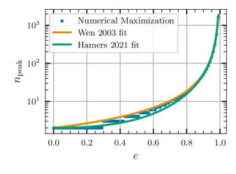
Figure 1: Numerical solution of Eq. (1) for the peak harmonic plotted along with the analytical fits from Ref. Wen (2003) and Ref. Hamers (2021). We see that the peak harmonic increases with eccentricity, and reaches values $>100$ for $e>0.9$. We also see that the fit in Ref. Hamers (2021) fits the numerical solution better, especially at lower values of eccentricity.

At least in the inspiral phase of the binary, i.e. when the dynamics is well-described by PN expansion, a binary emits GWs at harmonics of its orbital frequency $f_{\mathrm{orb}}$,

$$f_{\mathrm{GW},n}=nf_{\mathrm{orb}}\mbox{\quad;\quad}n\geq 2\mbox{\quad.\quad}$$

Note that the harmonic index $n$ is different from the $(\ell,m)$ basis used to parametrize GW polarizations. At leading order, power emitted by the $n$-th harmonic is given by Peters and Mathews (1963),

$$P_{n}=\frac{32}{5}\frac{G^{4}}{c^{5}}\frac{m_{1}^{2}m_{2}^{2}M}{a^{5}}g(n,e),$$ (1)

where the function $g(n,e)$ quantifies the enhancement in the power emitted in the $n^{\mathrm{th}}$ harmonic compared to a circular orbit (where there is no emission at $n>2$), and is given by

$$g(n,e)=\frac{n^{4}}{32}\biggl{\{}\biggl{[}J_{n-2}(ne)-2eJ_{n-1}(ne)+\frac{2}{n}J_{n}(ne)$$

$$\quad+2eJ_{n+1}(ne)-J_{n+2}(ne)\biggl{]}^{2}+\left(1-e^{2}\right)\biggl{[}J_{n-2}(ne)$$

$$\quad-2J_{n}(ne)+J_{n+2}(ne)\biggl{]}^{2}+\frac{4}{3n^{2}}J_{n}(ne)^{2}\biggl{\}}.$$ (2)

Here, $J_{k}(x)$ refers to Bessel functions of the first kind. For a given eccentricity, the peak power is emitted at a harmonic where $g(n,e)$ has the maximum value. For ease of calculation, Ref. Wen (2003) provided a fit to the peak harmonic as a function of eccentricity,

$$n^{\mathrm{Wen}}_{\mathrm{peak}}(e)=2\dfrac{(1+e)^{1.1954}}{(1-e^{2})^{3/2}}\mbox{\quad.\quad}$$ (3)

Ref. Hamers (2021) noted that the above fit does not work well at low eccentricities, and provided an alternative fit to the peak harmonic,

$$n^{\mathrm{Hamers}}_{\mathrm{peak}}(e)=2\quantity(1+\sum_{k=1}^{4}c_{k}e^{k}){(1-e^{2})^{-3/2}}\mbox{\quad.\quad}$$ (4)

Here, $c_{1}=-1.01678$, $c_{2}=5.57372$, $c_{3}=-4.9271$, and $c_{4}=1.68506$. Both these estimates are plotted in Figure 1 along with the peak harmonic calculated numerically.

II.2 Eccentricity extraction prescription of Ref. Wen (2003)

Since the value of eccentricity changes during the course of the inspiral, the value of eccentricity is often quoted at a specific reference frequency (or reference time). Ref. Wen (2003) (henceforth referred to as W03) uses the peak harmonic’s frequency as a reference for defining eccentricity, and this definition has been employed by many other studies (e.g. Samsing and Ramirez-Ruiz (2017); Samsing (2018); Rodriguez et al. (2018a); Zevin et al. (2019, 2021b); Kritos et al. (2022); Chattopadhyay et al. (2023)). Given semimajor axis $a$ and total mass $M$, the average orbital frequency $f_{\mathrm{orb}}$ is

$$f_{\mathrm{orb}}=\dfrac{1}{2\pi}\sqrt{\dfrac{GM}{a^{3}}}\mbox{\quad.\quad}$$ (5)

This means that the peak GW frequency is,

$$f_{\mathrm{peak,GW}}=\dfrac{(1+e)^{1.1954}}{\pi(1-e^{2})^{3/2}}\sqrt{\dfrac{GM}{a^{3}}}\mbox{\quad.\quad}$$ (6)

In astrophysical simulations, we are generally interested in obtaining eccentricity at a specified reference frequency, given an initial value of semi-major axis $a_{0}$ and eccentricity $e_{0}$. These initial values can be thought of as arising either from some fiducial distribution of eccentricities and separations, or from stopping conditions in dynamical simulations. W03 uses the leading (Newtonian) order evolution Peters (1964) of the semi-major axis and eccentricity to relate $(a_{0},e_{0})$ to $(a,e)$ at a different time,

$$\dfrac{a(1-e^{2})}{e^{12/19}}\quantity(1+\dfrac{121}{304}e^{2})^{-870/2299}=\dfrac{a_{0}(1-e_{0}^{2})}{e_{0}^{12/19}}\quantity(1+\dfrac{121}{304}e_{0}^{2})^{-870/2299}\mbox{\quad.\quad}$$ (7)

For a given value of the reference frequency $f_{\rm peak,GW}$, the eccentricity can be obtained by solving Eq. (6) and Eq. (7) simultaneously.

II.3 Possible issues with the W03 prescription

While the W03 procedure has been used in deriving eccentricities at a particular GW frequency in many simulations, it has a couple of drawbacks:

1. The reference frequency is taken to be the peak frequency of the orbit. This is inconsistent with recommendations in the literature attempting to standardize the definition of eccentricity in waveforms Ramos-Buades et al. (2022); Shaikh et al. (2023). Specfically, these works motivate using the orbit-averaged 22 (i.e. $\ell=2$, $m=2$) mode frequency as a consistent reference point, on account of its smooth and monotonic evolution over the course of the inspiral.

2. Since all equations are based on Ref. Peters (1964), they are restricted to Newtonian (i.e. leading) order. This is not a good approximation of the evolution of the orbit, especially for systems close to merger. Specifically, the ordinary differential equations describing the evolution of eccentricities and the 22 mode frequencies have been calculated to several PN orders beyond the Newtonian order, also with the inclusion of spins. Furthermore, this equation breaks down at very high eccentricity.

In the rest of our paper, we shall formulate a procedure that can be applied to any set of scattering experiments to extract eccentricities, and conduct sanity checks of our procedure. In order to accomplish this, we shall solve the problems listed above.

III A consistent prescription for calculating eccentricity

As shown in Figure 1, the peak harmonic of an eccentric inspiral takes higher values for higher eccentricities. For low values of eccentricity ($e\lesssim 0.3$), the peak harmonic is $n_{\rm peak}=2$, and hence the 22-mode frequency is the same as frequency of the peak harmonic. However, the difference between the peak harmonic frequency and the 22-mode frequency increases very quickly, with $f_{\rm peak}=10f_{\rm orb}=5f_{22}$ at $e\approx 0.7$. This discrepancy means that the eccentricities derived from astrophysical simulations of different binary formation channels is defined at a different reference frequency as compared to the definition of reference frequency built into waveforms as per recommendations of Ref. Shaikh et al. (2023). As is also evident, this discrepancy is worse for higher eccentricities, which are arguably more interesting from an astrophysical standpoint.

To remedy this discrepancy, the definitions of eccentricity from the simulations and waveforms need to be placed on the same footing. Hence, instead of defining eccentricity at the frequency of the peak harmonic, we define eccentricity at the orbit-averaged 22 mode frequency. Let $M=m_{1}+m_{2}$ be the total mass of the binary and $\eta=(m_{1}m_{2})/M^{2}$ be the symmetric mass ratio, where $m_{1}$ and $m_{2}$ are the component binary masses. Given an initial value of semimajor axis $a_{0}$ and eccentricity $e_{0}$ for a particular binary from a simulation, we evolve differential equations in $e$ and $v$ given by PN formulae,

$$\derivative{e}{t} =-\frac{e(121e^{2}+304)\eta v^{8}}{15M\epsilon^{5}}\quantity[1+\alpha_{2}v^{2}+\alpha_{3}v^{3}+\alpha_{4}v^{4}+\order{v^{5}}]$$ (8)

$$\derivative{v}{t} =\frac{\left(37e^{4}+292e^{2}+96\right)\eta v^{9}}{15M\epsilon^{7}}\quantity[1+\beta_{2}v^{2}+\beta_{3}v^{3}+\beta_{4}v^{4}+\order{v^{5}}]$$ (9)

$$f_{22} =\dfrac{v^{3}}{\pi M}$$ (10)

where $\epsilon=\sqrt{1-e^{2}}$, and $\alpha_{i}$, $\beta_{i}$ are PN coefficients that depend on $e$ and $\eta$ Peters (1964); Junker and Schaefer (1992); Rieth and Schäfer (1997); Gopakumar and Iyer (1997); Arun et al. (2009). For the purposes of this work, we will use equations accurate up to 2PN order (i.e. terms up to $\order{v^{4}}$), and will neglect the effect of spin. We note that the full expressions are known up to 3PN order Arun et al. (2009) including the effect of spin Henry and Khalil (2023), but we find that restricting to 2PN gives results accurate enough for our purposes. Evolving the above equations in time starting from the initial conditions, we extract eccentricities at an appropriate reference frequency. This way of defining eccentricity makes it consistent with the one defined in waveforms, modulo systematics in modeling the GW emission itself. In the next section, we compare estimates derived from the prescription mentioned above (which we denote by $e_{t}^{\rm 2PN}$) to the those derived from the W03 prescription (denoted as $e_{\rm W03}$) as used in the astrophysical simulations literature, and also investigate potential biases due to incomplete physics.

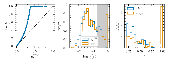
Figure 2: Comparison of orbital eccentricities in CMC simulations derived using the W03 prescription ($e_{\rm W03}$), to ones derived using the prescription in this work ($e_{t}^{\rm 2PN}$). The left panel shows a scatter plot of the two quantities. We see that there is considerable disagreement on the derived values of eccentricity, especially at $e\gtrsim 0.2$. This can be understood as the effect of the peak frequencies being shifted to higher $n_{\mathrm{peak}}$. The middle panel shows the histogram of (log) eccentricities for GW captures in globular clusters that occur during strong, few-body resonating interactions, derived using the W03 prescription and the prescription described in this work. The histograms do not deviate significantly from each other at low values of eccentricity, but are significantly different at $e\gtrsim 0.2$ (shaded region). The right panel shows the histogram of eccentricities in this $e\gtrsim 0.2$ region, where the discrepancies are more evident. Notably, the peak at $e\approx 1$ is no longer present in the histogram; this peak is an artifact of the procedure used to extract eccentricity in astrophysical simulations.

III.1 Comparison with the W03 prescription

As an illustration of our prescription, we consider binary mergers simulated with the Cluster Monte Carlo (CMC) code Rodriguez et al. (2022). CMC performs long-term evolution of a globular cluster using a Hénon type Monte Carlo algorithm Hénon (1971a, b); Joshi et al. (2000, 2001); Fregeau et al. (2003); Fregeau and Rasio (2007); Chatterjee et al. (2010, 2013); Pattabiraman et al. (2013); Rodriguez et al. (2015) given a set of initial conditions for the cluster. While we will only consider the CMC simulations as an example in this section, we again note that the W03 prescription has been in many other works (see e.g. Samsing and Ramirez-Ruiz (2017); Samsing (2018); Rodriguez et al. (2018a); Zevin et al. (2019); Kritos et al. (2022); Chattopadhyay et al. (2023)).

A catalog of CMC simulations on a grid of initial cluster masses, metallicity, radii, and galactocentric distances is publicly available Kremer et al. (2020, 2020). This catalog also includes information about compact object mergers that take place in these clusters. Merging compact binaries are extracted from these simulations using the following procedure:

1. During strong GW encounters, the approximated $N$-body dynamics (including leading-order PN corrections that account for orbital energy dissipation from GW emission Rodriguez et al. (2018b)) is evolved until two of the compact objects are in a bound state and reach a critical separation (typically $100M$), at which point the binary is assumed to definitively lead to a GW-driven merger and the properties of the binary are recorded.

2. With this pair of eccentricity and semimajor axis, the eccentricity at a given reference frequency is extracted using the prescription of W03.

Instead of relying on the W03 definition of eccentricity, we apply the procedure outlined in Section III to each binary extracted from the simulations. We then calculate eccentricities at a fixed 22-mode reference frequency of 10 Hz. In the upper panel of Figure 2, we show a scatter plot of eccentricities derived from the two different definitions. Here, $e_{\rm W03}$ corresponds to the eccentricity as calculated by the W03 prescription, whereas $e_{t}^{\rm 2PN}$ corresponds to the one calculated using the prescription presented in this work. At low eccentricities, the two definitions agree with each other. However, as one increases the eccentricity, the disagreement between the two increases quite rapidly. This is a direct result of the peak frequency getting shifted to higher harmonics as one increases eccentricity; for higher eccentricity, a given peak frequency $f_{\rm peak,GW}$ will correspond to a lower $f_{22}$ (since $\frac{1}{2}n_{\rm peak}f_{22}=f_{\rm peak,GW}$), hence describing the $e_{t}^{\rm 2PN}$ at a much lower reference frequency. This also means that the binary will lose more of its eccentricity by the time it reaches $f_{\rm 22}=10\,{\rm Hz}$. As a consequence, $e_{t}^{\rm 2PN}$ is always less than $e_{\rm W03}$.

Notably, all the points that have $e_{\rm W03}\approx 1$ have $e_{t}^{\rm 2PN}$ that range from $0.4-0.8$. We note that in many places in the literature, this $e\approx 1$ peak has been interpreted to be binaries that form “in-band” and merge quickly after getting captured; these are classically hyperbolic systems that are captured with a periapse frequency above the reference frequency considered (e.g., 10 Hz) via orbital energy loss through GW emission. While that interpretation still remains qualitatively correct, our analysis shows that the value of eccentricity that should be supplied to waveforms in comparison studies is not $e\approx 1$ but rather is shifted to much lower values.

The middle panel of Figure 2 shows histograms of $e_{\rm W03}$ and $e_{t}^{\rm 2PN}$ calculated from the CMC simulations, with appropriate weights applied to each sample based on cluster mass, metallicity, and detection probability. As would be expected from the preceding discussions, the histograms match for low values of eccentricity, and start deviating at $e\gtrsim 0.2$. Most strikingly, the peak at $e_{\rm W03}\approx 1$ in the $e_{\rm W03}$ histogram is not present in the $e_{t}^{\rm 2PN}$ histogram. These observations are more evident in the right panel of Figure 2, where we show the histograms of eccentricities for $e>0.2$. Since the waveform changes significantly as a function of eccentricity, one would expect these discrepancies to impact any analysis that assumes consistency between the definitions of eccentricities in waveforms and astrophysical simulations. We will comment on this briefly in Section III.4.

In the preceding discussion, we have assumed that the reference frequency is defined in the source-frame of the binary as opposed to the detector-frame. We make this choice since the original calculation of eccentricity using the W03 prescription with the CMC outputs made this choice. Strictly, this is incorrect and adds another significant level of inconsistency in the conventions for eccentricity. For completeness, we also show the eccentricity extracted at a reference frequency corresponding to a constant $f_{\rm 22}M=1000\,{\rm Hz}M_{\odot}$ in Figure 3, as $f_{\rm 22}M$ does not depend on redshift. At a $f_{\rm 22}$ corresponding to constant $f_{\rm 22}M$, all (black hole) binaries would be at the same epoch in their orbital evolution, i.e. they will all be at a fixed number of cycles before merger. This criterion is easy to implement while estimating parameters from BBH signals, and also allows for a more direct comparison of eccentricities for systems with different masses.

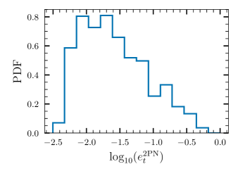
Figure 3: Histogram of eccentricities extracted at $Mf_{22}=1000\,M_{\odot}{\rm Hz}$. Defining the eccentricity at a fixed $Mf_{22}$ has a few advantages: (i) $Mf_{22}$ is independent of redshift, (ii) it defines eccentricity consistently at a fixed number of cycles before merger, and (iii) it is easy to implement while estimating source parameters from BBH signals. We recommend that all astrophysical simulations provide $e_{t}^{\rm 2PN}$ estimates extracted at a fixed $Mf_{22}$ for easy comparison with estimates of eccentricity derived using GW waveform models.

It is natural to ask whether the discrepancy is primarily driven by the mismatch in conventions for the reference frequency, or due to only accounting for the leading order PN term in the W03 prescription. The results in the preceding paragraphs would lead us to believe that it is the former. We test this in another way: since we know $n_{\rm peak}(e)$, we can also adjust the eccentricities calculated via W03 as a post-processing step by assuming that the $e_{\rm W03}$ is defined at a reference frequency $f_{\rm 22}=2\times f_{\rm peak}/n_{\rm peak}(e)$, and evolve to a fixed reference (22-mode) frequency using PN equations (Eqs. (8)-(10)) but only up to the leading order. Let the eccentricity calculated using this modified version of the W03 procedure be $e_{\rm W03}^{f_{22}}$. We find that $e_{\rm W03}^{f_{22}}\approx e_{t}^{\rm 2PN}$ for the binaries we consider, with a $\sim 5\%$ scatter that could be attributed to non-inclusion of higher-order PN terms (see also Section III.2). This further confirms that the discrepancy in the calculated eccentricities is primarily driven by the difference in conventions for the reference frequency.

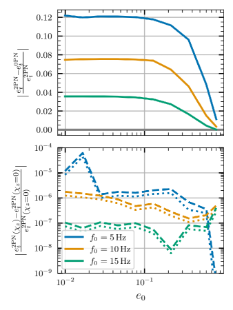
Figure 4: The top panel compares $e_{t}^{\rm 0PN}$ and $e_{t}^{\rm 2PN}$ computed at $f_{\mathrm{ref}}=20\,\rm Hz$ for three initial frequencies $f_{0}=5,10,15\,{\rm Hz}$ as a function of initial eccentricity $e_{0}$. The bottom panel makes a similar comparison between $e_{t}^{\rm 2PN}$ calculated assuming a value $\chi_{z}=\chi_{1,z}=\chi_{2,z}$, and $\chi_{z}=0$. We choose two representative values of $\chi_{z}$: $\chi_{z}=0.7$ (dotted lines), and $\chi_{z}=0.99$ (dashed lines).

III.2 Effects of ignoring higher order PN terms and spin effects

We now systematically investigate if there is a relative advantage in using the 2PN equations above just the leading order (0PN) evolution equations. For an equal mass binary of total mass $M=50\,M_{\odot}$, we consider three different starting frequencies $f_{0}=5,10,15\,{\rm Hz}$, and calculate $e_{t}^{\rm 2PN}$ and $e_{t}^{\rm 0PN}$ at a reference frequency of 20 Hz for a range of initial eccentricities $e_{0}$. The fractional differences between $e_{t}^{\rm 2PN}$ and $e_{t}^{\rm 0PN}$ estimates are plotted in the top panel of Figure 4, and show an increasing trend for lower values of $f_{0}$, with a discrepancy as high as $12\%$ for $f_{0}=5\,{\rm Hz}$. For a given $f_{0}$, the fractional differences are lower for higher $e_{0}$. In typical applications, one might want to calculate eccentricities at a given reference frequency for much lower values of $f_{0}$. While a $\sim 10\%$ difference might not be relevant while comparing eccentricity estimates from data to simulations, we recommend using $e_{t}^{\rm 2PN}$ estimates since the costs of evaluating $e_{t}^{\rm 0PN}$ and $e_{t}^{\rm 2PN}$ are similar (see Appendix C).

Our prescription in Section III does not include the effects of spin. To see if this is a valid choice, we use the same mass, $f_{0}$, $f_{\rm ref}$, and $e_{0}$ values as in the previous paragraph and calculate $e_{t}^{\rm 2PN}$ with and without including spin terms in the evolution for two representative dimensionless (aligned) spin values of $\chi_{1,z}=\chi_{2,z}=\chi_{z}=[0.7,\,0.99]$. For the spin terms in the evolution, we use 2PN accurate terms from Ref. Klein et al. (2018). The fractional differences between $e_{t}^{\rm 2PN}$ estimates with and without spin effects are shown in the lower panel of Figure 4. We see that the discrepancies are at worst $\sim 10^{-5}$, shifting to even lower values when considering smaller fiducial spins or higher $f_{0}$. We hence conclude that the non-spinning approximation is sufficient.

III.3 Comparison to estimates derived from gw_eccentricity package

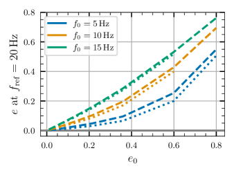
Figure 5: Comparison between the eccentricity definition given by Ref. Shaikh et al. (2023), calculated using the waveform approximant SEOBNRv4EHM ($e_{\rm gw}^{\rm SEOB}$; dotted lines), and $e_{t}^{\rm 2PN}$ (dashed lines), as a function of the initial eccentricity, $e_{0}$, for three initial frequencies, $f_{0}=5,10,15\,{\rm Hz}$. We assume an equal mass non-spinning binary with total mass $M=50\,M_{\odot}$ for this purpose.

As mentioned earlier, different GW waveform approximants have different conventions to define eccentricity. To solve this issue, Ref. Shaikh et al. (2023) proposed a standardized definition of eccentricity that can be applied to any waveform approximant, $e_{\rm gw}$, which is given by

$$e_{\rm gw}=\cos{\left(\Psi/3\right)}-\sqrt{3}\sin{\left(\Psi/3\right)}\;,$$ (11)

where

$$\Psi = \arctan{\left(\frac{1-e_{\omega_{22}}^{2}}{2e_{\omega_{22}}}\right)}\;,$$ (12)

$$e_{\omega_{22}}(t) = \frac{\sqrt{\omega_{22}^{\mathrm{p}}(t)}-\sqrt{\omega_{22}^{\mathrm{a}}(t)}}{\sqrt{\omega_{22}^{\mathrm{p}}(t)}+\sqrt{\omega_{22}^{\mathrm{a}}(t)}}\;,$$ (13)

and $\omega_{22}^{\rm p,a}(t)$ are the 22-mode frequencies through the pericenters and apocenters, respectively. This standardized definition is proposed in order to extract eccentricity directly from observables, in this case the gravitational waveform. More details on the motivations for this definition and the various methods of calculating $\omega_{22}^{\rm p,a}(t)$ can be found in Ref. Shaikh et al. (2023). We also briefly investigate the differences between $e_{\rm gw}$ derived from different waveform approximants in Appendix B.

While $e_{\rm gw}$ does asymptote to the PN definition of eccentricity, these two definitions may differ in general. For instance, waveforms could include more accurate dynamics at high eccentricity and closer to merger as compared to our 2PN prescription. Instead of the 2PN accurate equations, we could hence imagine replacing the prescription in Section III by generating waveforms at the specified initial epochs, and let gw_eccentricity calculate the eccentricities at the required reference frequency.

However, since calculating $e_{\rm gw}$ involves computing the waveform starting at a specified initial frequency/time, the calculation would be on the order of a hundred times slower (see Appendix C) than computing the PN eccentricity. The cost of generating waveforms also increases with decreasing starting frequency. Since astrophysical simulations require calculating eccentricites of a large number of binaries, calculating the Ref. Shaikh et al. (2023) definition of eccentricity would be computationally inefficient. Therefore, we now compare the differences between the two eccentricity definitions, $e_{\rm gw}$ and $e_{t}^{\rm 2PN}$, and quantify the reliability of $e_{t}^{\rm 2PN}$ eccentricity estimates from astrophysical simulations. For the investigations that follow, we will use the SEOBNRv4EHM Ramos-Buades et al. (2022) waveform approximant for the calculation of $e_{\rm gw}$. Using the same mass, $f_{0}$, and $e_{0}$ values as in Section III.2, we calculate $e_{t}^{\rm 2PN}$ and $e_{\rm gw}^{\rm SEOB}$ at a reference frequency of 20 Hz. Figure 5 illustrates the differences between these. While small (a few tens of a percent at worst), the differences do accumulate as the binary evolves for a longer period of time with $f_{0}$ values closer to the reference frequency giving more agreement. Since the cost of computing $e_{\rm gw}$ is a factor of $\sim 100$ greater as compared to calculating $e_{t}^{\rm 2PN}$ (see Appendix C), we conclude that $e_{t}^{\rm 2PN}$ is sufficient, especially in regimes where PN theory is valid.

III.4 Implications for existing work

A number of works have ascertained the detectability of eccentric mergers within the LVK band as well as in other detector bands, using data from astrophysical simulations such as CMC. As we have shown in the previous sections, the waveform eccentricities are not in agreement with the eccentricities given by simulations. Hence, we would expect these detectability estimates to change when defining eccentricity consistently in the simulations. For instance, Ref. Zevin et al. (2021b) found that $\approx$60% of potentially detectable eccentric sources with $e\gtrsim 0.2$ would be missed due to non-inclusion of eccentric templates in search pipelines. Using the same dataset as Ref. Zevin et al. (2021b) and changing the eccentricities from the $e_{\rm W03}$ definition to the $e_{t}^{\rm 2PN}$ definition, we find that only 30% of potentially detectable eccentric sources with $e\gtrsim 0.2$ are missed—a discrepancy by a factor of $\approx 2$. The decrease in the number of missed signals is due to the shifting of the histogram of eccentricities towards lower values, which are better approximated by non-eccentric templates and hence less likely to be selected against. As another illustration, we calculate limits on the cluster branching fraction $\beta_{c}$ i.e the fraction of events in the total population coming from clusters using the same method and dataset as used in Ref. Zevin et al. (2021a). We find that assuming $N_{\rm ecc}=0$ eccentric detections in GWTC-3, we would have inferred $\beta_{c}<86\%$ ($90\%$ credible level) using the $e_{\rm W03}$ estimates, and infer $\beta_{c}<63\%$ using the $e_{t}^{\rm 2PN}$ estimates. On the other hand, assuming $N_{\rm ecc}=1$ gives $\beta_{c}>10\%$ using the $e_{\rm W03}$ estimates and $\beta_{c}>8\%$ using the $e_{t}^{\rm 2PN}$ estimates.

Similarly, any study that uses the detected eccentricities (or lack thereof) to place constraints on the overall merger rate in eccentric systems in astrophysical environments will also be affected by these discrepancies. For instance, Ref. Abac et al. (2023) use the non-detection of orbital eccentricity from a waveform-independent search to place an upper limit of $0.34\,{\rm Gpc^{-3}\,{yr}^{-1}}$ on the merger rate of binaries in dense stellar clusters, assuming a population model from CMC simulations. This population model is taken from Ref. Zevin et al. (2021b) with eccentricities defined using the W03 prescription, with additional conditioning on the mass ($M>70$) and eccentricity ($e<0.3$) parameter ranges of their search. From Figure 2, we see that the relative number of mergers having $e<0.3$ increases when accounting for the prescription in this work. This means that an upper limit derived using the $e_{t}^{\rm 2PN}$ estimates from this work would be lower than the ones quoted in Ref. Abac et al. (2023).

We also note that Ref. Romero-Shaw et al. (2022), which uses signatures of non-zero eccentricity in four GW events to constrain the fraction of BBH mergers formed dynamically, does account for the disparate conventions for eccentricity while making their comparisons. They do so in an approximate fashion, similar to the calculation of $e_{\rm W03}^{f_{22}}$ described in Section III.1. We do not expect conclusions reported there to change significantly.

IV Conclusion

Orbital eccentricity in a compact binary is believed to be a telltale sign of its formation history. Consequently, there has been progress on building waveform models for eccentric sources as well as on simulating expectations from astrophysical formation channels. In this work, we note that the conventions used to define eccentricity in the GW waveform and astrophysical simulation communities differ from each other. The major difference in these conventions lies in the choice of the reference frequency at which eccentricity is defined—GW waveforms typically define eccentricity at a fixed orbit averaged 22-mode GW frequency, while astrophysical simulations define eccentricity at a fixed peak GW frequency following the W03 prescription (described in Section II.2). Further, we delineate an eccentricity calculation procedure that can be applied to data from astrophysical simulations to extract eccentricities consistent with conventions laid down by the GW waveform community. This procedure involves evolution of ordinary differential equations describing the time-evolution of eccentricity and frequency obtained from PN expansions, and extracting eccentricity consistently at the orbit-averaged 22 mode frequency.

Using compact binaries from the publicly-available CMC catalog as an illustration, we find that there is a discrepancy between eccentricity estimates derived using the W03 prescription and the one described in this work. The discrepancy is small for $e\lesssim 0.1$, but is large for higher values of eccentricity. Notably, all binaries with $e_{\rm W03}\approx 1$ (thought to be GW captures happening in the LVK band) have $e_{t}^{\rm 2PN}$ between $0.4$–$0.8$. We investigate the effect that adding 2PN corrections to the leading order evolution has on derived eccentricities, and also the effects of not including spins in our prescription. We also compare our $e_{t}^{\rm 2PN}$ estimates to $e_{\rm gw}$ estimates derived from the gw_eccentricity package using the SEOBNRv4EHM waveform. We find that the $e_{t}^{\rm 2PN}$ estimates should be sufficiently accurate in extracting eccentricities, and also computationally efficient to implement as a post-processing step in simulations. However, as outlined in Ref. Shaikh et al. (2023), gw_eccentricity is the most accurate way of extracting eccentricity and should be used when high-precision eccentricity estimates are necessary.

The different conventions for defining eccentricity currently employed in the literature mean that one should be careful in comparing eccentricity estimates/upper limits derived from real data to astrophysical simulations, creating mock populations of eccentric sources based on astrophysical expectations, and other investigations that pair predictions from astrophysical models with GW data analysis. As an illustration, we show that the detectability estimates of eccentric sources and branching fractions from Ref. Zevin et al. (2021b) will change when ensuring a consistent definition of eccentricity. We recommend that catalogs created from astrophysical simulations include $e_{t}^{\rm 2PN}$ estimates (extracted at a constant $Mf_{22}$) for clarity and ease of direct comparison to GW observations.

Appendix A PN formulae for eccentricity and velocity evolution

The PN formulae (accurate up to 2PN) for the evolution of eccentricity and velocity are given below

$$\derivative{e}{t} =-\frac{e(121e^{2}+304)\eta v^{8}}{15M\epsilon^{5}}\quantity[1+\alpha_{2}v^{2}+\alpha_{3}v^{3}+\alpha_{4}v^{4}+\order{v^{5}}]$$ (14)

$$\derivative{v}{t} =\frac{\left(37e^{4}+292e^{2}+96\right)\eta v^{9}}{15M\epsilon^{7}}\quantity[1+\beta_{2}v^{2}+\beta_{3}v^{3}+\beta_{4}v^{4}+\order{v^{5}}]$$ (15)

$$f_{22} =\dfrac{v^{3}}{\pi M}$$ (16)

where

$$\alpha_{2} =\frac{125361e^{4}+718008e^{2}-28\left(3328e^{4}+23259e^{2}+8168\right)\eta-67608}{168(121e+304)\epsilon^{2}}$$ (17)

$$\alpha_{3} =\frac{1970\pi v^{3}\epsilon^{5}}{121e+304}\phi_{e}^{\rm rad}$$ (18)

$$\alpha_{4} =\frac{1}{2016(121e+304)\epsilon^{4}}[3e^{6}\left(919520\eta^{2}-1448284\eta+1262181\right)$$

$$\mathrel{\phantom{=}}+e^{4}\left(42810096\eta^{2}-78343602\eta-569520(2\eta-5)\epsilon+46566110\right)$$

$$\mathrel{\phantom{=}}-12e^{2}(3495771\eta+584892(2\eta-5)\epsilon-945290)$$

$$\mathrel{\phantom{=}}-16\left(-284256\eta^{2}-801495\eta+168336(2\eta-5)\epsilon+952397\right)]$$ (19)

and

$$\beta_{2} =\dfrac{e^{6}(11717-8288\eta)+e^{4}(171038-141708\eta)-120e^{2}(1330\eta-731)+16(743-924\eta)}{56\left(37e^{4}+292e^{2}+96\right)\epsilon^{2}}$$ (20)

$$\beta_{3} =\frac{768\pi v^{3}\epsilon^{7}}{74e^{4}+584e^{2}+192}\phi_{e}$$ (21)

$$\beta_{4} =-\frac{1}{6048\left(37e^{4}+292e^{2}+96\right)\epsilon^{4}}[-3e^{8}\left(654752\eta^{2}-1086660\eta+1174371\right)$$

$$\mathrel{\phantom{=}}+6e^{6}\left(-10804808\eta^{2}+20518071\eta+88200(2\eta-5)\epsilon-13904067\right)$$

$$\mathrel{\phantom{=}}+12e^{4}\left(-13875505\eta^{2}+17267022\eta+1105272(2\eta-5)\epsilon-65314\right)$$

$$\mathrel{\phantom{=}}+16e^{2}\left(-3830127\eta^{2}-966546\eta+806652(2\eta-5)\epsilon+5802910\right)$$

$$\mathrel{\phantom{=}}+32\left(-59472\eta^{2}-141093\eta+9072(2\eta-5)\epsilon+11257\right)]\mbox{\quad.\quad}$$ (22)

Here, $\epsilon=\sqrt{1-e^{2}}$. Here, the “enhancement factors” $\phi_{e}$, $\tilde{\phi}_{e}$, and $\phi_{e}^{\rm rad}$ are given by

$$\phi_{e} =\frac{\frac{428340e^{12}}{9958749469}-\frac{5034498e^{10}}{7491716851}+\frac{9293260e^{8}}{3542508891}+\frac{48176523e^{6}}{177473701}+\frac{157473274e^{4}}{30734301}+\frac{18970894028e^{2}}{2649026657}+1}{\epsilon^{10}}$$ (23)

$$\tilde{\phi}_{e} =\frac{-\frac{328675e^{10}}{8674876481}-\frac{4679700e^{8}}{6316712563}-\frac{2640201e^{6}}{993226448}+\frac{37570495e^{4}}{98143337}+\frac{413137256e^{2}}{136292703}+1}{\epsilon^{9}}$$ (24)

$$\phi_{e}^{\rm rad} =\frac{192\epsilon(\epsilon\phi_{e}-\tilde{\phi}_{e})}{985e^{2}}\mbox{\quad.\quad}$$ (25)

Appendix B Variation in gw_eccentricity estimates calculated from different waveform approximants

The prescription of calculating eccentricity $e_{\rm gw}$, proposed by Shaikh et al. (2023) and implemented in the gw_eccentricity python package only uses the GW waveform as seen by the detector as input, as described in Section III.3. This definition is beneficial since eccentricity is now linked to a direct observable. However, different waveforms will, in general, yield different values of $e_{\rm gw}$ for the same binary. This could be due to a variety of reasons: differences in the modeling of the dynamics, different internal definitions of eccentricity in the model, or even choices made while implementing the approximant in some codebase such as LALSimulation LIGO Scientific Collaboration et al. (2018). Figure 6 illustrates this point by comparing $e_{\rm gw}$ derived from two waveforms, EccentricTD Tanay et al. (2016) and SEOBNRv4EHM Ramos-Buades et al. (2022). For this illustration, we assume an equal mass binary with a total mass of $M=50\,M_{\odot}$. We vary the initial eccentricity $e_{0}$ (defined at initial frequency $f_{0}=5\,{\rm Hz}$) supplied to the model between $10^{-2}$ and $0.8$, and extract $e_{\rm gw}$ from both EccentricTD $\quantity(e_{\rm gw}^{\rm EccTD})$ and SEOBNRv4EHM $\quantity(e_{\rm gw}^{\rm SEOB})$, at both the initial frequency $f_{0}$ and also at $f_{\rm ref}=20\,{\rm Hz}$. We see that $e_{\rm gw}^{\rm SEOB}(f_{0})$ matches all input values $e_{0}$, whereas $e_{\rm gw}^{\rm EccTD}(f_{0})$ differs from $e_{0}$ by a few percent. This is in agreement with investigations performed in Ref. Shaikh et al. (2023), where they found that the $e_{\rm gw}^{\rm SEOB}\quantity(f_{0})=e_{0}$ trend is maintained for all $e_{0}>10^{-5}$, whereas $e_{\rm gw}^{\rm EccTD}$ deviates from the $e_{\rm gw}^{\rm EccTD}\quantity(f_{0})=e_{0}$ trend. We also see that there is a large discrepancy (factor of a few) between $e_{\rm gw}^{\rm EccTD}(f_{\rm ref})$ and $e_{\rm gw}^{\rm SEOB}(f_{\rm ref})$, strengthening the evidence for differences in the ways each of these waveform approximants define eccentricity. We use the SEOBNRv4EHM approximant for our comparisons in Section III.3.

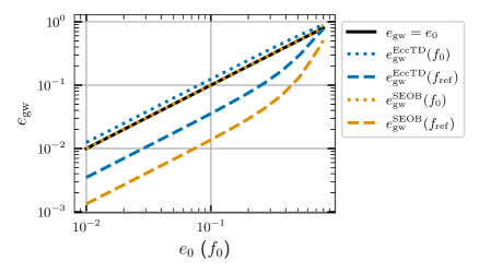
Figure 6: Comparison of internal definitions of eccentricity for different waveform models as a function of the initial input eccentricity, $e_{0}$ with a fiducial input frequency of 5 Hz. Initial eccentricities using the standardized definition, $e_{\rm gw}(f_{0})$ (dotted lines), should be consistent with the input eccentricity $e_{0}$ (black line). EccentricTD (blue) does not agree for any value of $e_{0}$, while SEOBNRv4EHM (yellow) does agree for all $e_{0}$ values considered. We also see that the final eccentricity reported for the given reference frequency $f_{\mathrm{ref}}$ between the two waveforms (blue and yellow dashed lines) do not agree.

Appendix C Computational cost of different eccentricity prescriptions

Astrophysical simulations keep track of many evolving binary systems, where it is often computationally infeasible to compute waveforms for all systems. In Figure 7, we demonstrate the speed-up in eccentricity calculation at the reference frequency, $f_{\rm ref}$, by computing the PN eccentricities, $e_{t}^{k{\rm PN}}$, as opposed to the standardized waveform definition of eccentricity, $e_{\rm gw}$. The top left of Figure 7 demonstrates the average time to compute the 2PN eccentricity at various initial eccentricities, $e_{0}$, and frequencies, $f_{0}$. The top right plot illustrates that computing the waveform eccentricity, $e_{\rm gw}$ using the SEOBNRv4EHM waveform model takes on the order of a hundred times longer on average. The bottom plots in Figure 7 demonstrate that using the 0PN eccentricity has a comparable cost to using the 2PN eccentricity, whereas including spin effects in the PN equations is $\sim$1.5 times slower.

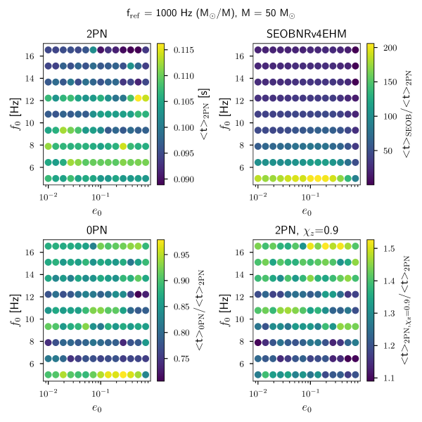
Figure 7: Average time to compute the 2PN eccentricity (top left) and the relative time to compute the eccentricities using the SEOBNRv4EHM waveform (top right), the 0PN eccentricity (bottom left), and the 2PN eccentricity for spinning binaries (bottom right). The grid covers various input eccentricity, $e_{0}$, and frequency, $f_{0}$, values. Calculating eccentricities using waveforms takes $\sim 100\times$ longer than calculating eccentricities using our PN approximation.

References

References

- LIGO Scientific Collaboration et al. (2015) LIGO Scientific Collaboration, J. Aasi, B. P. Abbott, R. Abbott, T. Abbott, M. R. Abernathy, K. Ackley, C. Adams, T. Adams, P. Addesso, et al., “Advanced LIGO,” Classical and Quantum Gravity 32, 074001 (2015), arXiv:1411.4547 [gr-qc] .
- Acernese et al. (2015) F. Acernese, M. Agathos, K. Agatsuma, D. Aisa, N. Allemandou, A. Allocca, J. Amarni, P. Astone, G. Balestri, G. Ballardin, et al., “Advanced Virgo: a second-generation interferometric gravitational wave detector,” Classical and Quantum Gravity 32, 024001 (2015), arXiv:1408.3978 [gr-qc] .
- Aso et al. (2013) Yoichi Aso, Yuta Michimura, Kentaro Somiya, Masaki Ando, Osamu Miyakawa, Takanori Sekiguchi, Daisuke Tatsumi, and Hiroaki Yamamoto, “Interferometer design of the KAGRA gravitational wave detector,” Phys. Rev. D 88, 043007 (2013), arXiv:1306.6747 [gr-qc] .
- Akutsu et al. (2021) T. Akutsu, M. Ando, K. Arai, Y. Arai, S. Araki, A. Araya, N. Aritomi, Y. Aso, S. Bae, Y. Bae, L. Baiotti, R. Bajpai, M. A. Barton, K. Cannon, E. Capocasa, M. Chan, C. Chen, K. Chen, Y. Chen, H. Chu, Y. K. Chu, S. Eguchi, Y. Enomoto, R. Flaminio, Y. Fujii, M. Fukunaga, M. Fukushima, G. Ge, A. Hagiwara, S. Haino, K. Hasegawa, H. Hayakawa, K. Hayama, Y. Himemoto, Y. Hiranuma, N. Hirata, E. Hirose, Z. Hong, B. H. Hsieh, C. Z. Huang, P. Huang, Y. Huang, B. Ikenoue, S. Imam, K. Inayoshi, Y. Inoue, K. Ioka, Y. Itoh, K. Izumi, K. Jung, P. Jung, T. Kajita, M. Kamiizumi, N. Kanda, G. Kang, K. Kawaguchi, N. Kawai, T. Kawasaki, C. Kim, J. C. Kim, W. S. Kim, Y. M. Kim, N. Kimura, N. Kita, H. Kitazawa, Y. Kojima, K. Kokeyama, K. Komori, A. K. H. Kong, K. Kotake, C. Kozakai, R. Kozu, R. Kumar, J. Kume, C. Kuo, H. S. Kuo, S. Kuroyanagi, K. Kusayanagi, K. Kwak, H. K. Lee, H. W. Lee, R. Lee, M. Leonardi, L. C. C. Lin, C. Y. Lin, F. L. Lin, G. C. Liu, L. W. Luo, M. Marchio, Y. Michimura, N. Mio, O. Miyakawa, A. Miyamoto, Y. Miyazaki, K. Miyo, S. Miyoki, S. Morisaki, Y. Moriwaki, K. Nagano, S. Nagano, K. Nakamura, H. Nakano, M. Nakano, R. Nakashima, T. Narikawa, R. Negishi, W. T. Ni, A. Nishizawa, Y. Obuchi, W. Ogaki, J. J. Oh, S. H. Oh, M. Ohashi, N. Ohishi, M. Ohkawa, K. Okutomi, K. Oohara, C. P. Ooi, S. Oshino, K. Pan, H. Pang, J. Park, F. E. Peña Arellano, I. Pinto, N. Sago, S. Saito, Y. Saito, K. Sakai, Y. Sakai, Y. Sakuno, S. Sato, T. Sato, T. Sawada, T. Sekiguchi, Y. Sekiguchi, S. Shibagaki, R. Shimizu, T. Shimoda, K. Shimode, H. Shinkai, T. Shishido, A. Shoda, K. Somiya, E. J. Son, H. Sotani, R. Sugimoto, T. Suzuki, T. Suzuki, H. Tagoshi, H. Takahashi, R. Takahashi, A. Takamori, S. Takano, H. Takeda, M. Takeda, H. Tanaka, K. Tanaka, K. Tanaka, T. Tanaka, T. Tanaka, S. Tanioka, E. N. Tapia San Martin, S. Telada, T. Tomaru, Y. Tomigami, T. Tomura, F. Travasso, L. Trozzo, T. Tsang, K. Tsubono, S. Tsuchida, T. Tsuzuki, D. Tuyenbayev, N. Uchikata, T. Uchiyama, A. Ueda, T. Uehara, K. Ueno, G. Ueshima, F. Uraguchi, T. Ushiba, M. H. P. M. van Putten, H. Vocca, J. Wang, C. Wu, H. Wu, S. Wu, W. R. Xu, T. Yamada, K. Yamamoto, K. Yamamoto, T. Yamamoto, K. Yokogawa, J. Yokoyama, T. Yokozawa, T. Yoshioka, H. Yuzurihara, S. Zeidler, Y. Zhao, and Z. H. Zhu, “Overview of KAGRA: Detector design and construction history,” Progress of Theoretical and Experimental Physics 2021, 05A101 (2021), arXiv:2005.05574 [physics.ins-det] .
- Abbott et al. (2018) B. P. Abbott, R. Abbott, T. D. Abbott, M. R. Abernathy, F. Acernese, K. Ackley, C. Adams, T. Adams, P. Addesso, R. X. Adhikari, et al., “Prospects for observing and localizing gravitational-wave transients with Advanced LIGO, Advanced Virgo and KAGRA,” Living Reviews in Relativity 21, 3 (2018), arXiv:1304.0670 [gr-qc] .
- Abbott et al. (2023a) R. Abbott, T. D. Abbott, F. Acernese, K. Ackley, C. Adams, N. Adhikari, R. X. Adhikari, V. B. Adya, C. Affeldt, D. Agarwal, et al., “GWTC-3: Compact Binary Coalescences Observed by LIGO and Virgo during the Second Part of the Third Observing Run,” Physical Review X 13, 041039 (2023a), arXiv:2111.03606 [gr-qc] .
- Abbott et al. (2023b) R. Abbott, T. D. Abbott, F. Acernese, K. Ackley, C. Adams, N. Adhikari, R. X. Adhikari, V. B. Adya, C. Affeldt, D. Agarwal, M. Agathos, K. Agatsuma, N. Aggarwal, O. D. Aguiar, L. Aiello, A. Ain, P. Ajith, T. Akutsu, P. F. de Alarcón, S. Akcay, S. Albanesi, A. Allocca, P. A. Altin, A. Amato, C. Anand, S. Anand, A. Ananyeva, S. B. Anderson, W. G. Anderson, M. Ando, T. Andrade, N. Andres, T. Andrić, S. V. Angelova, S. Ansoldi, J. M. Antelis, S. Antier, F. Antonini, S. Appert, Koji Arai, Koya Arai, Y. Arai, S. Araki, A. Araya, M. C. Araya, LIGO Scientific Collaboration, VIRGO Collaboration, and KAGRA Collaboration, “Population of Merging Compact Binaries Inferred Using Gravitational Waves through GWTC-3,” Physical Review X 13, 011048 (2023b), arXiv:2111.03634 [astro-ph.HE] .
- Zevin et al. (2021a) Michael Zevin, Simone S. Bavera, Christopher P. L. Berry, Vicky Kalogera, Tassos Fragos, Pablo Marchant, Carl L. Rodriguez, Fabio Antonini, Daniel E. Holz, and Chris Pankow, “One Channel to Rule Them All? Constraining the Origins of Binary Black Holes Using Multiple Formation Pathways,” ApJ 910, 152 (2021a), arXiv:2011.10057 [astro-ph.HE] .
- Cheng et al. (2023) April Qiu Cheng, Michael Zevin, and Salvatore Vitale, “What You Don’t Know Can Hurt You: Use and Abuse of Astrophysical Models in Gravitational-wave Population Analyses,” ApJ 955, 127 (2023), arXiv:2307.03129 [astro-ph.HE] .
- O’Leary et al. (2009) Ryan M. O’Leary, Bence Kocsis, and Abraham Loeb, “Gravitational waves from scattering of stellar-mass black holes in galactic nuclei,” MNRAS 395, 2127–2146 (2009), arXiv:0807.2638 [astro-ph] .
- Kocsis and Levin (2012) Bence Kocsis and Janna Levin, “Repeated bursts from relativistic scattering of compact objects in galactic nuclei,” Phys. Rev. D 85, 123005 (2012), arXiv:1109.4170 [astro-ph.CO] .
- Samsing et al. (2014) Johan Samsing, Morgan MacLeod, and Enrico Ramirez-Ruiz, “The Formation of Eccentric Compact Binary Inspirals and the Role of Gravitational Wave Emission in Binary-Single Stellar Encounters,” ApJ 784, 71 (2014), arXiv:1308.2964 [astro-ph.HE] .
- Antonini et al. (2017) Fabio Antonini, Silvia Toonen, and Adrian S. Hamers, “Binary Black Hole Mergers from Field Triples: Properties, Rates, and the Impact of Stellar Evolution,” ApJ 841, 77 (2017), arXiv:1703.06614 [astro-ph.GA] .
- Samsing and Ramirez-Ruiz (2017) Johan Samsing and Enrico Ramirez-Ruiz, “On the Assembly Rate of Highly Eccentric Binary Black Hole Mergers,” ApJ 840, L14 (2017), arXiv:1703.09703 [astro-ph.HE] .
- Silsbee and Tremaine (2017) Kedron Silsbee and Scott Tremaine, “Lidov-Kozai Cycles with Gravitational Radiation: Merging Black Holes in Isolated Triple Systems,” ApJ 836, 39 (2017), arXiv:1608.07642 [astro-ph.HE] .
- Rodriguez et al. (2018a) Carl L. Rodriguez, Pau Amaro-Seoane, Sourav Chatterjee, Kyle Kremer, Frederic A. Rasio, Johan Samsing, Claire S. Ye, and Michael Zevin, “Post-Newtonian dynamics in dense star clusters: Formation, masses, and merger rates of highly-eccentric black hole binaries,” Phys. Rev. D 98, 123005 (2018a), arXiv:1811.04926 [astro-ph.HE] .
- Rodriguez and Antonini (2018) Carl L. Rodriguez and Fabio Antonini, “A Triple Origin for the Heavy and Low-spin Binary Black Holes Detected by LIGO/VIRGO,” ApJ 863, 7 (2018), arXiv:1805.08212 [astro-ph.HE] .
- Samsing (2018) Johan Samsing, “Eccentric black hole mergers forming in globular clusters,” Phys. Rev. D 97, 103014 (2018), arXiv:1711.07452 [astro-ph.HE] .
- Samsing et al. (2018a) Johan Samsing, Abbas Askar, and Mirek Giersz, “MOCCA-SURVEY Database. I. Eccentric Black Hole Mergers during Binary-Single Interactions in Globular Clusters,” ApJ 855, 124 (2018a), arXiv:1712.06186 [astro-ph.HE] .
- Samsing et al. (2018b) Johan Samsing, Daniel J. D’Orazio, Abbas Askar, and Mirek Giersz, “Black Hole Mergers from Globular Clusters Observable by LISA and LIGO: Results from post-Newtonian Binary-Single Scatterings,” arXiv e-prints , arXiv:1802.08654 (2018b), arXiv:1802.08654 [astro-ph.HE] .
- Fragione and Kocsis (2019) Giacomo Fragione and Bence Kocsis, “Black hole mergers from quadruples,” MNRAS 486, 4781–4789 (2019), arXiv:1903.03112 [astro-ph.GA] .
- Fragione and Bromberg (2019) Giacomo Fragione and Omer Bromberg, “Eccentric binary black hole mergers in globular clusters hosting intermediate-mass black holes,” MNRAS 488, 4370–4377 (2019), arXiv:1903.09659 [astro-ph.GA] .
- Liu et al. (2019) Bin Liu, Dong Lai, and Yi-Han Wang, “Black Hole and Neutron Star Binary Mergers in Triple Systems. II. Merger Eccentricity and Spin-Orbit Misalignment,” ApJ 881, 41 (2019), arXiv:1905.00427 [astro-ph.HE] .
- Liu and Lai (2019) Bin Liu and Dong Lai, “Enhanced black hole mergers in binary-binary interactions,” MNRAS 483, 4060–4069 (2019), arXiv:1809.07767 [astro-ph.HE] .
- Zevin et al. (2019) Michael Zevin, Johan Samsing, Carl Rodriguez, Carl-Johan Haster, and Enrico Ramirez-Ruiz, “Eccentric Black Hole Mergers in Dense Star Clusters: The Role of Binary-Binary Encounters,” ApJ 871, 91 (2019), arXiv:1810.00901 [astro-ph.HE] .
- Michaely and Perets (2020) Erez Michaely and Hagai B. Perets, “High rate of gravitational waves mergers from flyby perturbations of wide black hole triples in the field,” MNRAS 498, 4924–4935 (2020), arXiv:2008.01094 [astro-ph.HE] .
- Gondán and Kocsis (2021) László Gondán and Bence Kocsis, “High eccentricities and high masses characterize gravitational-wave captures in galactic nuclei as seen by Earth-based detectors,” MNRAS 506, 1665–1696 (2021), arXiv:2011.02507 [astro-ph.HE] .
- Tagawa et al. (2021) Hiromichi Tagawa, Bence Kocsis, Zoltán Haiman, Imre Bartos, Kazuyuki Omukai, and Johan Samsing, “Eccentric Black Hole Mergers in Active Galactic Nuclei,” ApJ 907, L20 (2021), arXiv:2010.10526 [astro-ph.HE] .
- Mapelli et al. (2021) Michela Mapelli, Marco Dall’Amico, Yann Bouffanais, Nicola Giacobbo, Manuel Arca Sedda, M. Celeste Artale, Alessandro Ballone, Ugo N. Di Carlo, Giuliano Iorio, Filippo Santoliquido, and Stefano Torniamenti, “Hierarchical black hole mergers in young, globular and nuclear star clusters: the effect of metallicity, spin and cluster properties,” MNRAS 505, 339–358 (2021), arXiv:2103.05016 [astro-ph.HE] .
- Zevin et al. (2021b) Michael Zevin, Isobel M. Romero-Shaw, Kyle Kremer, Eric Thrane, and Paul D. Lasky, “Implications of Eccentric Observations on Binary Black Hole Formation Channels,” ApJ 921, L43 (2021b), arXiv:2106.09042 [astro-ph.HE] .
- Zhang et al. (2021) Fupeng Zhang, Xian Chen, Lijing Shao, and Kohei Inayoshi, “The Eccentric and Accelerating Stellar Binary Black Hole Mergers in Galactic Nuclei: Observing in Ground and Space Gravitational-wave Observatories,” ApJ 923, 139 (2021), arXiv:2109.14842 [astro-ph.HE] .
- Samsing et al. (2022) J. Samsing, I. Bartos, D. J. D’Orazio, Z. Haiman, B. Kocsis, N. W. C. Leigh, B. Liu, M. E. Pessah, and H. Tagawa, “AGN as potential factories for eccentric black hole mergers,” Nature 603, 237–240 (2022), arXiv:2010.09765 [astro-ph.HE] .
- Trani et al. (2022) Alessandro A. Trani, Sara Rastello, Ugo N. Di Carlo, Filippo Santoliquido, Ataru Tanikawa, and Michela Mapelli, “Compact object mergers in hierarchical triples from low-mass young star clusters,” MNRAS 511, 1362–1372 (2022), arXiv:2111.06388 [astro-ph.HE] .
- Dall’Amico et al. (2023) Marco Dall’Amico, Michela Mapelli, Stefano Torniamenti, and Manuel Arca Sedda, “Eccentric black hole mergers via three-body interactions in young, globular and nuclear star clusters,” arXiv e-prints , arXiv:2303.07421 (2023), arXiv:2303.07421 [astro-ph.HE] .
- Romero-Shaw et al. (2023a) Isobel Romero-Shaw, Nicholas Loutrel, and Michael Zevin, “Inferring interference: Identifying a perturbing tertiary with eccentric gravitational wave burst timing,” Phys. Rev. D 107, 122001 (2023a), arXiv:2211.07278 [gr-qc] .
- Peters (1964) P. C. Peters, “Gravitational Radiation and the Motion of Two Point Masses,” Physical Review 136, 1224–1232 (1964).
- von Zeipel (1910) H. von Zeipel, “Sur l’application des séries de M. Lindstedt à l’étude du mouvement des comètes périodiques,” Astronomische Nachrichten 183, 345 (1910).
- Lidov (1962) M.L. Lidov, “The evolution of orbits of artificial satellites of planets under the action of gravitational perturbations of external bodies,” Planetary and Space Science 9, 719–759 (1962).
- Kozai (1962) Yoshihide Kozai, “Secular perturbations of asteroids with high inclination and eccentricity,” AJ 67, 591–598 (1962).
- Sachdev et al. (2019) Surabhi Sachdev, Sarah Caudill, Heather Fong, Rico K. L. Lo, Cody Messick, Debnandini Mukherjee, Ryan Magee, Leo Tsukada, Kent Blackburn, Patrick Brady, Patrick Brockill, Kipp Cannon, Sydney J. Chamberlin, Deep Chatterjee, Jolien D. E. Creighton, Patrick Godwin, Anuradha Gupta, Chad Hanna, Shasvath Kapadia, Ryan N. Lang, Tjonnie G. F. Li, Duncan Meacher, Alexander Pace, Stephen Privitera, Laleh Sadeghian, Leslie Wade, Madeline Wade, Alan Weinstein, and Sophia Liting Xiao, “The GstLAL Search Analysis Methods for Compact Binary Mergers in Advanced LIGO’s Second and Advanced Virgo’s First Observing Runs,” arXiv e-prints , arXiv:1901.08580 (2019), arXiv:1901.08580 [gr-qc] .
- Davies et al. (2020) Gareth S. Davies, Thomas Dent, Márton Tápai, Ian Harry, Connor McIsaac, and Alexander H. Nitz, “Extending the PyCBC search for gravitational waves from compact binary mergers to a global network,” Phys. Rev. D 102, 022004 (2020), arXiv:2002.08291 [astro-ph.HE] .
- Aubin et al. (2021) F. Aubin, F. Brighenti, R. Chierici, D. Estevez, G. Greco, G. M. Guidi, V. Juste, F. Marion, B. Mours, E. Nitoglia, O. Sauter, and V. Sordini, “The MBTA pipeline for detecting compact binary coalescences in the third LIGO-Virgo observing run,” Classical and Quantum Gravity 38, 095004 (2021), arXiv:2012.11512 [gr-qc] .
- Abbott et al. (2019) B. P. Abbott, R. Abbott, T. D. Abbott, S. Abraham, F. Acernese, K. Ackley, A. Adams, C. Adams, R. X. Adhikari, V. B. Adya, and oithers, “Search for intermediate mass black hole binaries in the first and second observing runs of the Advanced LIGO and Virgo network,” Phys. Rev. D 100, 064064 (2019), arXiv:1907.09384 [astro-ph.HE] .
- Abac et al. (2023) A. G. Abac, R. Abbott, H. Abe, F. Acernese, K. Ackley, C. Adamcewicz, S. Adhicary, et al., “Search for Eccentric Black Hole Coalescences during the Third Observing Run of LIGO and Virgo,” arXiv e-prints , arXiv:2308.03822 (2023), arXiv:2308.03822 [astro-ph.HE] .
- Tanay et al. (2016) Sashwat Tanay, Maria Haney, and Achamveedu Gopakumar, “Frequency and time-domain inspiral templates for comparable mass compact binaries in eccentric orbits,” Phys. Rev. D 93, 064031 (2016), arXiv:1602.03081 [gr-qc] .
- Huerta et al. (2018) E. A. Huerta, C. J. Moore, Prayush Kumar, Daniel George, Alvin J. K. Chua, Roland Haas, Erik Wessel, Daniel Johnson, Derek Glennon, Adam Rebei, A. Miguel Holgado, Jonathan R. Gair, and Harald P. Pfeiffer, “Eccentric, nonspinning, inspiral, Gaussian-process merger approximant for the detection and characterization of eccentric binary black hole mergers,” Phys. Rev. D 97, 024031 (2018), arXiv:1711.06276 [gr-qc] .
- Nagar et al. (2021) Alessandro Nagar, Alice Bonino, and Piero Rettegno, “Effective one-body multipolar waveform model for spin-aligned, quasicircular, eccentric, hyperbolic black hole binaries,” Phys. Rev. D 103, 104021 (2021), arXiv:2101.08624 [gr-qc] .
- Ramos-Buades et al. (2022) Antoni Ramos-Buades, Alessandra Buonanno, Mohammed Khalil, and Serguei Ossokine, “Effective-one-body multipolar waveforms for eccentric binary black holes with nonprecessing spins,” Phys. Rev. D 105, 044035 (2022), arXiv:2112.06952 [gr-qc] .
- Liu et al. (2022) Xiaolin Liu, Zhoujian Cao, and Zong-Hong Zhu, “A higher-multipole gravitational waveform model for an eccentric binary black holes based on the effective-one-body-numerical-relativity formalism,” Classical and Quantum Gravity 39, 035009 (2022), arXiv:2102.08614 [gr-qc] .
- Liu et al. (2023) Xiaolin Liu, Zhoujian Cao, and Zong-Hong Zhu, “Effective-One-Body Numerical-Relativity waveform model for Eccentric spin-precessing binary black hole coalescence,” arXiv e-prints , arXiv:2310.04552 (2023), arXiv:2310.04552 [gr-qc] .
- Klein (2021) Antoine Klein, “EFPE: Efficient fully precessing eccentric gravitational waveforms for binaries with long inspirals,” arXiv e-prints , arXiv:2106.10291 (2021), arXiv:2106.10291 [gr-qc] .
- Romero-Shaw et al. (2023b) Isobel M. Romero-Shaw, Davide Gerosa, and Nicholas Loutrel, “Eccentricity or spin precession? Distinguishing subdominant effects in gravitational-wave data,” MNRAS 519, 5352–5357 (2023b), arXiv:2211.07528 [astro-ph.HE] .
- Xu and Hamilton (2023) Yumeng Xu and Eleanor Hamilton, “Measurability of precession and eccentricity for heavy binary-black-hole mergers,” Phys. Rev. D 107, 103049 (2023), arXiv:2211.09561 [gr-qc] .
- Romero-Shaw et al. (2020) Isobel Romero-Shaw, Paul D. Lasky, Eric Thrane, and Juan Calderón Bustillo, “GW190521: Orbital Eccentricity and Signatures of Dynamical Formation in a Binary Black Hole Merger Signal,” ApJ 903, L5 (2020), arXiv:2009.04771 [astro-ph.HE] .
- Knee et al. (2022) Alan M. Knee, Isobel M. Romero-Shaw, Paul D. Lasky, Jess McIver, and Eric Thrane, “A Rosetta Stone for Eccentric Gravitational Waveform Models,” ApJ 936, 172 (2022), arXiv:2207.14346 [gr-qc] .
- Bonino et al. (2023) Alice Bonino, Rossella Gamba, Patricia Schmidt, Alessandro Nagar, Geraint Pratten, Matteo Breschi, Piero Rettegno, and Sebastiano Bernuzzi, “Inferring eccentricity evolution from observations of coalescing binary black holes,” Phys. Rev. D 107, 064024 (2023), arXiv:2207.10474 [gr-qc] .
- Shaikh et al. (2023) Md Arif Shaikh, Vijay Varma, Harald P. Pfeiffer, Antoni Ramos-Buades, and Maarten van de Meent, “Defining eccentricity for gravitational wave astronomy,” Phys. Rev. D 108, 104007 (2023), arXiv:2302.11257 [gr-qc] .
- Vijaykumar et al. (2024) Aditya Vijaykumar, Alexandra G. Hanselman, and Michael Zevin, “Data release for "Consistent eccentricities for gravitational wave astronomy: Resolving discrepancies between astrophysical simulations and waveform models",” (2024).
- Wen (2003) Linqing Wen, “On the Eccentricity Distribution of Coalescing Black Hole Binaries Driven by the Kozai Mechanism in Globular Clusters,” ApJ 598, 419–430 (2003), arXiv:astro-ph/0211492 [astro-ph] .
- Kritos et al. (2022) Konstantinos Kritos, Vladimir Strokov, Vishal Baibhav, and Emanuele Berti, “Rapster: a fast code for dynamical formation of black-hole binaries in dense star clusters,” arXiv e-prints , arXiv:2210.10055 (2022), arXiv:2210.10055 [astro-ph.HE] .
- Chattopadhyay et al. (2023) Debatri Chattopadhyay, Jakob Stegmann, Fabio Antonini, Jordan Barber, and Isobel M. Romero-Shaw, “Double black hole mergers in nuclear star clusters: eccentricities, spins, masses, and the growth of massive seeds,” MNRAS 526, 4908–4928 (2023), arXiv:2308.10884 [astro-ph.HE] .
- Klein et al. (2018) Antoine Klein, Yannick Boetzel, Achamveedu Gopakumar, Philippe Jetzer, and Lorenzo de Vittori, “Fourier domain gravitational waveforms for precessing eccentric binaries,” Phys. Rev. D 98, 104043 (2018), arXiv:1801.08542 [gr-qc] .
- Hamers (2021) Adrian S. Hamers, “An Improved Numerical Fit to the Peak Harmonic Gravitational Wave Frequency Emitted by an Eccentric Binary,” Research Notes of the American Astronomical Society 5, 275 (2021), arXiv:2111.08033 [gr-qc] .
- Peters and Mathews (1963) P. C. Peters and J. Mathews, “Gravitational Radiation from Point Masses in a Keplerian Orbit,” Physical Review 131, 435–440 (1963).
- Fumagalli and Gerosa (2023) Giulia Fumagalli and Davide Gerosa, “Spin-eccentricity interplay in merging binary black holes,” Phys. Rev. D 108, 124055 (2023), arXiv:2310.16893 [gr-qc] .
- Junker and Schaefer (1992) Wolfgang Junker and Gerhard Schaefer, “Binary systems - Higher order gravitational radiation damping and wave emission,” MNRAS 254, 146–164 (1992).
- Rieth and Schäfer (1997) Ronald Rieth and Gerhard Schäfer, “Spin and tail effects in the gravitational-wave emission of compact binaries,” Classical and Quantum Gravity 14, 2357–2380 (1997).
- Gopakumar and Iyer (1997) A. Gopakumar and Bala R. Iyer, “Gravitational waves from inspiraling compact binaries: Angular momentum flux, evolution of the orbital elements, and the waveform to the second post-Newtonian order,” Phys. Rev. D 56, 7708–7731 (1997), arXiv:gr-qc/9710075 [gr-qc] .
- Arun et al. (2009) K. G. Arun, Luc Blanchet, Bala R. Iyer, and Siddhartha Sinha, “Third post-Newtonian angular momentum flux and the secular evolution of orbital elements for inspiralling compact binaries in quasi-elliptical orbits,” Phys. Rev. D 80, 124018 (2009), arXiv:0908.3854 [gr-qc] .
- Henry and Khalil (2023) Quentin Henry and Mohammed Khalil, “Spin effects in gravitational waveforms and fluxes for binaries on eccentric orbits to the third post-Newtonian order,” Phys. Rev. D 108, 104016 (2023), arXiv:2308.13606 [gr-qc] .
- Rodriguez et al. (2022) Carl L. Rodriguez, Newlin C. Weatherford, Scott C. Coughlin, Pau Amaro-Seoane, Katelyn Breivik, Sourav Chatterjee, Giacomo Fragione, Fulya Kıroğlu, Kyle Kremer, Nicholas Z. Rui, Claire S. Ye, Michael Zevin, and Frederic A. Rasio, “Modeling Dense Star Clusters in the Milky Way and beyond with the Cluster Monte Carlo Code,” ApJS 258, 22 (2022), arXiv:2106.02643 [astro-ph.GA] .
- Hénon (1971a) M. Hénon, “Monte Carlo Models of Star Clusters (Part of the Proceedings of the IAU Colloquium No. 10, held in Cambridge, England, August 12-15, 1970.),” Ap&SS 13, 284–299 (1971a).
- Hénon (1971b) M. H. Hénon, “The Monte Carlo Method (Papers appear in the Proceedings of IAU Colloquium No. 10 Gravitational N-Body Problem (ed. by Myron Lecar), R. Reidel Publ. Co. , Dordrecht-Holland.),” (1971) pp. 151–167.
- Joshi et al. (2000) Kriten J. Joshi, Frederic A. Rasio, and Simon Portegies Zwart, “Monte Carlo Simulations of Globular Cluster Evolution. I. Method and Test Calculations,” ApJ 540, 969–982 (2000), arXiv:astro-ph/9909115 [astro-ph] .
- Joshi et al. (2001) Kriten J. Joshi, Cody P. Nave, and Frederic A. Rasio, “Monte Carlo Simulations of Globular Cluster Evolution. II. Mass Spectra, Stellar Evolution, and Lifetimes in the Galaxy,” ApJ 550, 691–702 (2001), arXiv:astro-ph/9912155 [astro-ph] .
- Fregeau et al. (2003) J. M. Fregeau, M. A. Gürkan, K. J. Joshi, and F. A. Rasio, “Monte Carlo Simulations of Globular Cluster Evolution. III. Primordial Binary Interactions,” ApJ 593, 772–787 (2003), arXiv:astro-ph/0301521 [astro-ph] .
- Fregeau and Rasio (2007) John M. Fregeau and Frederic A. Rasio, “Monte Carlo Simulations of Globular Cluster Evolution. IV. Direct Integration of Strong Interactions,” ApJ 658, 1047–1061 (2007), arXiv:astro-ph/0608261 [astro-ph] .
- Chatterjee et al. (2010) Sourav Chatterjee, John M. Fregeau, Stefan Umbreit, and Frederic A. Rasio, “Monte Carlo Simulations of Globular Cluster Evolution. V. Binary Stellar Evolution,” ApJ 719, 915–930 (2010), arXiv:0912.4682 [astro-ph.GA] .
- Chatterjee et al. (2013) Sourav Chatterjee, Stefan Umbreit, John M. Fregeau, and Frederic A. Rasio, “Understanding the dynamical state of globular clusters: core-collapsed versus non-core-collapsed,” MNRAS 429, 2881–2893 (2013), arXiv:1207.3063 [astro-ph.GA] .
- Pattabiraman et al. (2013) Bharath Pattabiraman, Stefan Umbreit, Wei-keng Liao, Alok Choudhary, Vassiliki Kalogera, Gokhan Memik, and Frederic A. Rasio, “A Parallel Monte Carlo Code for Simulating Collisional N-body Systems,” ApJS 204, 15 (2013), arXiv:1206.5878 [astro-ph.IM] .
- Rodriguez et al. (2015) Carl L. Rodriguez, Meagan Morscher, Bharath Pattabiraman, Sourav Chatterjee, Carl-Johan Haster, and Frederic A. Rasio, “Binary Black Hole Mergers from Globular Clusters: Implications for Advanced LIGO,” Phys. Rev. Lett. 115, 051101 (2015), arXiv:1505.00792 [astro-ph.HE] .
- Kremer et al. (2020) Kyle Kremer, Claire S. Ye, Nicholas Z. Rui, Newlin C. Weatherford, Sourav Chatterjee, Giacomo Fragione, Carl L. Rodriguez, Mario Spera, and Frederic A. Rasio, “Modeling Dense Star Clusters in the Milky Way and Beyond with the CMC Cluster Catalog,” ApJS 247, 48 (2020), arXiv:1911.00018 [astro-ph.HE] .
- Kremer et al. (2020) Kyle Kremer, S Ye Claire, Nicholas Z Rui, Newlin C Weatherford, Sourav Chatterjee, Giacomo Fragione, Carl L Rodriguez, Mario Spera, and Frederic A Rasio, “Cluster monte carlo simulations,” (2020), accessed on 1-1-2023.
- Rodriguez et al. (2018b) Carl L. Rodriguez, Pau Amaro-Seoane, Sourav Chatterjee, and Frederic A. Rasio, “Post-Newtonian Dynamics in Dense Star Clusters: Highly Eccentric, Highly Spinning, and Repeated Binary Black Hole Mergers,” Phys. Rev. Lett. 120, 151101 (2018b), arXiv:1712.04937 [astro-ph.HE] .
- Romero-Shaw et al. (2022) Isobel Romero-Shaw, Paul D. Lasky, and Eric Thrane, “Four Eccentric Mergers Increase the Evidence that LIGO-Virgo-KAGRA’s Binary Black Holes Form Dynamically,” ApJ 940, 171 (2022), arXiv:2206.14695 [astro-ph.HE] .
- Harris et al. (2020) Charles R. Harris, K. Jarrod Millman, Stéfan J. van der Walt, Ralf Gommers, Pauli Virtanen, David Cournapeau, Eric Wieser, Julian Taylor, Sebastian Berg, Nathaniel J. Smith, Robert Kern, Matti Picus, Stephan Hoyer, Marten H. van Kerkwijk, Matthew Brett, Allan Haldane, Jaime Fernández del Río, Mark Wiebe, Pearu Peterson, Pierre Gérard-Marchant, Kevin Sheppard, Tyler Reddy, Warren Weckesser, Hameer Abbasi, Christoph Gohlke, and Travis E. Oliphant, “Array programming with NumPy,” Nature 585, 357–362 (2020), arXiv:2006.10256 [cs.MS] .
- Virtanen et al. (2020) Pauli Virtanen, Ralf Gommers, Travis E. Oliphant, Matt Haberland, Tyler Reddy, David Cournapeau, Evgeni Burovski, Pearu Peterson, Warren Weckesser, Jonathan Bright, Stéfan J. van der Walt, Matthew Brett, Joshua Wilson, K. Jarrod Millman, Nikolay Mayorov, Andrew R. J. Nelson, Eric Jones, Robert Kern, Eric Larson, C. J. Carey, İlhan Polat, Yu Feng, Eric W. Moore, Jake VanderPlas, Denis Laxalde, Josef Perktold, Robert Cimrman, Ian Henriksen, E. A. Quintero, Charles R. Harris, Anne M. Archibald, Antônio H. Ribeiro, Fabian Pedregosa, Paul van Mulbregt, and SciPy 1. 0 Contributors, “SciPy 1.0: fundamental algorithms for scientific computing in Python,” Nature Methods 17, 261–272 (2020), arXiv:1907.10121 [cs.MS] .
- Hunter (2007) John D. Hunter, “Matplotlib: A 2D Graphics Environment,” Computing in Science and Engineering 9, 90–95 (2007).
- Astropy Collaboration et al. (2013) Astropy Collaboration, Thomas P. Robitaille, Erik J. Tollerud, Perry Greenfield, Michael Droettboom, Erik Bray, Tom Aldcroft, Matt Davis, Adam Ginsburg, Adrian M. Price-Whelan, Wolfgang E. Kerzendorf, Alexander Conley, Neil Crighton, Kyle Barbary, Demitri Muna, Henry Ferguson, Frédéric Grollier, Madhura M. Parikh, Prasanth H. Nair, Hans M. Unther, Christoph Deil, Julien Woillez, Simon Conseil, Roban Kramer, James E. H. Turner, Leo Singer, Ryan Fox, Benjamin A. Weaver, Victor Zabalza, Zachary I. Edwards, K. Azalee Bostroem, D. J. Burke, Andrew R. Casey, Steven M. Crawford, Nadia Dencheva, Justin Ely, Tim Jenness, Kathleen Labrie, Pey Lian Lim, Francesco Pierfederici, Andrew Pontzen, Andy Ptak, Brian Refsdal, Mathieu Servillat, and Ole Streicher, “Astropy: A community Python package for astronomy,” A&A 558, A33 (2013), arXiv:1307.6212 [astro-ph.IM] .
- Astropy Collaboration et al. (2018) Astropy Collaboration, A. M. Price-Whelan, B. M. Sipőcz, H. M. Günther, P. L. Lim, S. M. Crawford, S. Conseil, D. L. Shupe, M. W. Craig, N. Dencheva, A. Ginsburg, J. T. VanderPlas, L. D. Bradley, D. Pérez-Suárez, M. de Val-Borro, T. L. Aldcroft, K. L. Cruz, T. P. Robitaille, E. J. Tollerud, C. Ardelean, T. Babej, Y. P. Bach, M. Bachetti, A. V. Bakanov, S. P. Bamford, G. Barentsen, P. Barmby, A. Baumbach, K. L. Berry, F. Biscani, M. Boquien, K. A. Bostroem, L. G. Bouma, G. B. Brammer, E. M. Bray, H. Breytenbach, H. Buddelmeijer, D. J. Burke, G. Calderone, J. L. Cano Rodríguez, M. Cara, J. V. M. Cardoso, S. Cheedella, Y. Copin, L. Corrales, D. Crichton, D. D’Avella, C. Deil, É. Depagne, J. P. Dietrich, A. Donath, M. Droettboom, N. Earl, T. Erben, S. Fabbro, L. A. Ferreira, T. Finethy, R. T. Fox, L. H. Garrison, S. L. J. Gibbons, D. A. Goldstein, R. Gommers, J. P. Greco, P. Greenfield, A. M. Groener, F. Grollier, A. Hagen, P. Hirst, D. Homeier, A. J. Horton, G. Hosseinzadeh, L. Hu, J. S. Hunkeler, Ž. Ivezić, A. Jain, T. Jenness, G. Kanarek, S. Kendrew, N. S. Kern, W. E. Kerzendorf, A. Khvalko, J. King, D. Kirkby, A. M. Kulkarni, A. Kumar, A. Lee, D. Lenz, S. P. Littlefair, Z. Ma, D. M. Macleod, M. Mastropietro, C. McCully, S. Montagnac, B. M. Morris, M. Mueller, S. J. Mumford, D. Muna, N. A. Murphy, S. Nelson, G. H. Nguyen, J. P. Ninan, M. Nöthe, S. Ogaz, S. Oh, J. K. Parejko, N. Parley, S. Pascual, R. Patil, A. A. Patil, A. L. Plunkett, J. X. Prochaska, T. Rastogi, V. Reddy Janga, J. Sabater, P. Sakurikar, M. Seifert, L. E. Sherbert, H. Sherwood-Taylor, A. Y. Shih, J. Sick, M. T. Silbiger, S. Singanamalla, L. P. Singer, P. H. Sladen, K. A. Sooley, S. Sornarajah, O. Streicher, P. Teuben, S. W. Thomas, G. R. Tremblay, J. E. H. Turner, V. Terrón, M. H. van Kerkwijk, A. de la Vega, L. L. Watkins, B. A. Weaver, J. B. Whitmore, J. Woillez, V. Zabalza, and Astropy Contributors, “The Astropy Project: Building an Open-science Project and Status of the v2.0 Core Package,” AJ 156, 123 (2018), arXiv:1801.02634 [astro-ph.IM] .
- Kluyver et al. (2016) Thomas Kluyver, Benjain Ragan-Kelley, Fernando Pérez, Brian Granger, Matthias Bussonnier, Jonathan Frederic, Kyle Kelley, Jessica Hamrick, Jason Grout, Sylvain Corlay, Paul Ivanov, Damián Avila, Safia Abdalla, Carol Willing, and Jupyter Development Team, “Jupyter Notebooks—a publishing format for reproducible computational workflows,” in IOS Press (IOS Press, 2016) pp. 87–90.
- McKinney (2010) Wes McKinney, “Data Structures for Statistical Computing in Python,” in Proceedings of the 9th Python in Science Conference, edited by Stéfan van der Walt and Jarrod Millman (2010) pp. 56 – 61.
- Waskom (2021) Michael Waskom, “seaborn: statistical data visualization,” The Journal of Open Source Software 6, 3021 (2021).
- LIGO Scientific Collaboration et al. (2018) LIGO Scientific Collaboration, Virgo Collaboration, and KAGRA Collaboration, “LVK Algorithm Library - LALSuite,” Free software (GPL) (2018).