Label-Efficient Model Selection for Text Generation

Label-Efficient Model Selection for Text Generation

Shir Ashury-Tahan^♠♡, Benjamin Sznajder^♠, Leshem Choshen^♠♢, Liat Ein-Dor^♠, Eyal Shnarch^♠ and Ariel Gera^{♠ ♠}IBM Research, ^♡Bar-Ilan University, ^♢MIT

1 Abstract

Model selection for a given target task can be costly, as it may entail extensive annotation of the quality of outputs of different models. We introduce DiffUse, an efficient method to make an informed decision between candidate text generation models. DiffUse reduces the required amount of preference annotations, thus saving valuable time and resources in performing evaluation.

DiffUse intelligently selects instances by clustering embeddings that represent the semantic differences between model outputs. Thus, it is able to identify a subset of examples that are more informative for preference decisions. Our method is model-agnostic, and can be applied to any text generation model. Moreover, we propose a practical iterative approach for dynamically determining how many instances to annotate. In a series of experiments over hundreds of model pairs, we demonstrate that DiffUse can dramatically reduce the required number of annotations – by up to $75\%$ – while maintaining high evaluation reliability.

2 Introduction

Model evaluation is a prerequisite for informed decisions – predominantly, choosing the right model for the task. As such, an essential requirement is the ability to compare models based on how well they perform.

Comparing model performance generally requires some sort of oracle – a human annotator or LLM-based evaluator – that can judge model outputs and prefer one output over another. However, depending on the nature of the oracle, such judgments can incur significant costs, particularly in terms of annotation budgets (Ein-Dor et al., 2020b; van der Lee et al., 2019) and computational requirements (Liang et al., 2022; Biderman et al., 2023; Perlitz et al., 2023a). Specifically for text generation tasks, the oracle is burdened with making nuanced judgments of the quality of generated texts (Celikyilmaz et al., 2020); often, this can only be done by expert human annotators (van der Lee et al., 2021), or possibly by powerful LLMs (e.g., GPT-4, Zheng et al., 2023), both of which are costly to apply at scale. Moreover, as the number of models and tasks increases, conducting these evaluations becomes prohibitively expensive (Perlitz et al., 2023a).

Our goal is to address the costs associated with evaluating model outputs in text generation, by reducing the burden on the oracle. Specifically, we focus on the use case of directly comparing two candidate models, where the oracle is asked to make preference judgements between the outputs generated by the two models. Our focus is on comparative judgments and not absolute scores, as these are considered more reliable for evaluating text generation (Callison-Burch et al., 2007; Sedoc et al., 2019; Li et al., 2019; Liang et al., 2020).

In this work, we propose a method that substantially reduces the number of examples that must be annotated by the oracle, while yielding a more reliable estimate of the preferred model for the task. Our approach - DiffUse - selects pairs of model outputs that on the one hand are representative of the space of differences between model behaviors on a given task, and on the other hand are more informative, showing clearer preference. Specifically, we calculate embedding vectors that represent the semantic difference between the outputs of the two models; then, by partitioning these embeddings into clusters, we can intelligently select a diverse informative subset of instances for annotation.

DiffUse is inherently generic and does not assume anything about the models, tasks, or unlabeled test data. Our results (§6) demonstrate its stability and effectiveness for different text generation tasks, across hundreds of pairs of generative models, and across a broad range of annotation budgets. We also propose an iterative real-world solution for practitioners (§6.2), which enables making reliable and cost-efficient choices between candidate models. We find this method to be better in all of our experiments, achieving a reduction in annotations of up to $75\%$ compared to random sampling.

Furthermore, we conduct a comprehensive analysis (§7) of the components of our method. Our findings suggest that our method tends to select examples from regions in the output-difference space that are dominated by the preferred model.

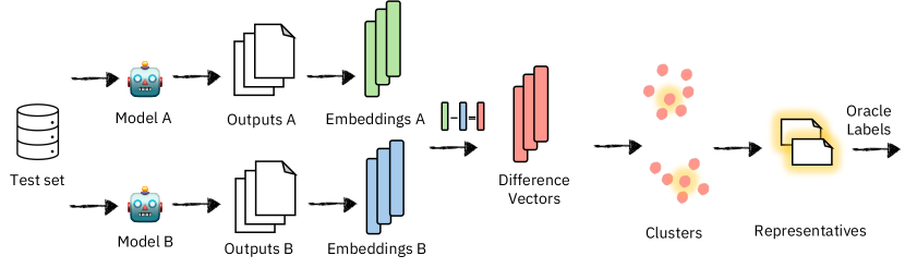
Figure 1: DiffUse flow. Our method consists of $5$ steps: performing inference with the models on the test set, encoding the generated outputs, performing pairwise subtraction, clustering the resulting vectors, and selecting representatives for evaluation. A comprehensive description is provided in §4.

3 Definitions and Problem Formulation

In this work, we focus on comparative evaluation of models. Given two text generation models, we wish to evaluate which model is stronger with respect to a given generation task, based on preference labels of an oracle over the model outputs.

For an input instance $x$ and a pair of models $M_{A}$,$M_{B}$ with corresponding outputs $y_{A}$,$y_{B}$, a preference label $y_{\text{pref}}\in\{M_{A},M_{B},T\}$ indicates whether $y_{A}$ is better than $y_{B}$ ($M_{A}$), worse than $y_{B}$ ($M_{B}$) or similar to $y_{B}$ ($T$).

Test winning model

The model for which the outputs over the test set $D_{\text{test}}$ are more frequently preferred by the oracle. Formally:

$$W_{\text{test}}=\begin{cases}M_{A}&\text{if }P^{M_{A}}_{\text{test}}>P^{M_{B}}_{\text{test}}\\ M_{B}&\text{if }P^{M_{A}}_{\text{test}}<P^{M_{B}}_{\text{test}}\\ T&\text{if }P^{M_{A}}_{\text{test}}=P^{M_{B}}_{\text{test}}\end{cases}$$

where

$$P^{m}_{\text{test}}=\frac{1}{|D_{\text{test}}|}\sum_{(x,y_{\text{pref}})\in D_{\text{test}}}\mathds{1}_{\{y_{\text{pref}}=m\}}$$ (1)

is the test winning probability of model $m\in\{M_{A},M_{B}\}$, and $\mathds{1}_{\{y_{\text{pref}}=m\}}$ is the indicator function that takes the value $1$ if $y_{\text{pref}}=m$ and $0$ otherwise.

Test winning distance

The absolute difference between the test winning probabilities of the two models, $|P^{M_{A}}_{\text{test}}-P^{M_{B}}_{\text{test}}|$.

Problem formulation

Calculating the test winning model requires preference labels for every point in the test set. However, this is often costly and impractical. Thus, our goal is to maximize the probability of identifying the test winning model under a given annotation budget, by wisely selecting only a subset of examples $D_{\text{test}}^{\text{observed}}\subseteq D_{\text{test}}$ from the test set to be labeled by the oracle.

A naive baseline for estimating the test winning model is to uniformly sample $N$ test instances, label them, and compute the winning model over these instances.

4 Method

Our algorithm, DiffUse, is simple and effective, and relies solely on the outputs generated by the models. The full flow is described in Figure 1.

We aim to represent examples in a manner that captures the distribution of model mismatching behaviors, i.e., various types of differences between model outputs. To this end, we first embed model outputs into a semantic vector space (using off-the-shelf methods). Subsequently, we generate difference vectors by subtracting the embeddings of one model from the embeddings of the other, for each example in the test set. Then, we cluster these difference vectors and select one representative from each cluster to be labeled by the oracle.

Given the construction of the difference vectors, we expect this vector space to largely carry information about semantic differences, i.e., the nature of disagreements between models. Choosing an example from each cluster ensures that the set of selected examples is representative of this space; hence, these examples are expected to be informative for estimating which is the preferred model.

5 Experiments

5.1 The Data

Throughout our experiments, we utilize data from the HELM benchmark (Liang et al., 2022, version 0.2.2). We rely on data from its core scenarios, which encompass inputs, outputs, and scores for various models, datasets, and tasks.

The HELM scores serve as the ground-truth data, such that the test winning model (§3) for a given scenario and model pair is the one that received a higher score for a greater number of test instances. Note that the scores within HELM reflect the result of an automated reference-based metric. Thus, while this “oracle” is not a human, it does rely on the existence of annotated human reference answers. Moreover, for each scenario we report results for several automated metrics, hence simulating a range of different kinds of oracles.

Our experimental setup includes $6$ text generation scenarios, with results of $666$ unique pairs of models (paired comparisons of $37$ different models) for each scenario. The tasks we experimented with are summarization and question answering (i.e., the text generation tasks in HELM), as detailed in Appendix Table 1. As shown in Fig. 2, the winning distances between model pairs in HELM span a large range, but are often small; in other words, HELM showcases diverse behaviors but determining the winning model is usually not trivial.

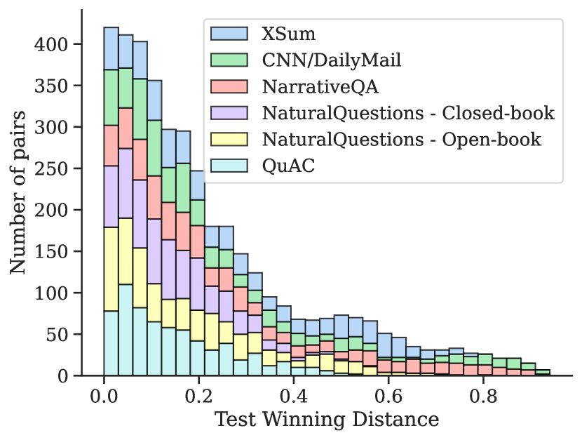
Figure 2: Distribution of test winning distance (§3) in HELM between pairs of generative models. Evidently, most models are closely positioned to each other.

5.2 Example Selection Method

As outlined above (§4), DiffUse consists of calculating difference vectors that represent the model output behaviors, clustering them, and sampling examples based on the resulting clusters.

Specifically, we use Sentence-BERT (Reimers and Gurevych, 2019) all-MiniLM-L6-v2 encoder to embed the outputs, and subtract the resulting embeddings to obtain difference vectors. For clustering the vectors, we opt for Hierarchical Agglomerative Clustering (Müllner, 2011) with Ward linkage and Euclidean distance.

For a given budget of $N$ examples to be annotated by the oracle, we select them by partitioning the vectors into $N$ clusters. Then, from each cluster we select a single example, and specifically the one whose embedding is closest (in cosine distance) to the center of the cluster.

Note that while we found this setup to work particularly well, opting for a different choice of clustering algorithm, or for a different approach of selecting examples given the clusters, does not dramatically affect the results (§7.1).

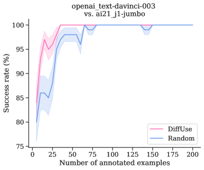
(a)

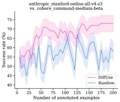
(b)

Figure 3: Comparing example selection methods. Success rates (± standard error) in identifying the best of two competing generative models (listed in the plot title), in terms of their performance over CNN/DailyMail (using Rouge-2 as the oracle).

5.3 Example Selection Experiments

Our main experiments examine the success rate of an example selection method, defined as follows.

For a given dataset, a budget of size $N$, and a pair of generative models, we use a selection method to select $N$ examples for annotation. This sample is then annotated by the oracle, and used to determine the sample winning model. An example selection run is succcessful when the sample winning model equals the test winning model. These binary results are then aggregated across several random seeds and across all generative model pairs to determine the success rate of the example selection method.

DiffUse is compared to the (strong) baseline of random selection, where the $N$ examples are sampled i.i.d. from the dataset.

To better estimate the robustness of the selection methods, for each experimental run (seed) we sample a large subset of the full data ($800$ out of $1000$ scenario examples in HELM) and treat this subset as if it were the full test set.

In total, for each of the $6$ HELM scenarios, we report results across $666$ unique model pairs, $10$ runs (seeds) for each, and varying $N$ between $5$ to $200$ examples to be annotated.

6 Results

We start by comparing the success rate of DiffUse to that of the Random selection baseline.

Figure 3 illustrates two cases of such comparison, each for a specific pair of models. As can be seen, success rates can vary greatly between cases where there is a relatively large performance difference between the generative models (left panel) and those with a small performance difference (right panel). As for the latter, estimating the preferred model is harder and requires more annotated instances. Naturally, the model preference estimation becomes more accurate as the budget $N$ increases and the preference decision relies on a larger set of examples annotated with oracle preference.

In the two cases presented in Fig. 3, DiffUse achieves higher success rates at identifying the better generative model, in comparison to random sampling. These results showcase that with DiffUse one can reach the correct decision with a smaller number of examples to be annotated by the oracle.

To give a broader and quantitative picture, Figure 4 depicts the aggregated results for the CNN/DailyMail summarization data, averaged across all $666$ model pairs. The plot demonstrates a clear advantage of our approach over random selection, arriving at the correct decision more often and using fewer examples. Thus, using DiffUse there is a much lower risk of choosing the wrong model. This pattern is quite consistent across the different datasets tested, as can be seen in Appendix A.1.

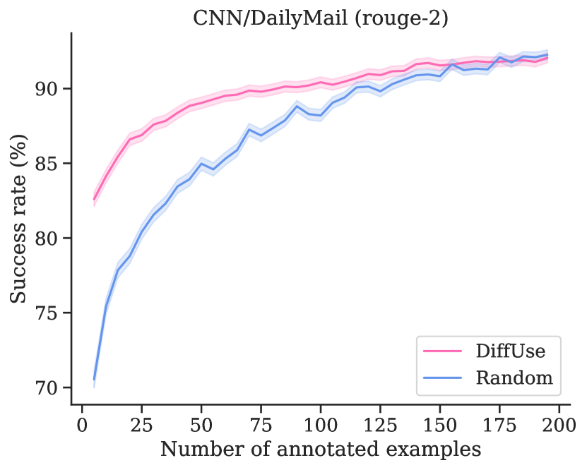
Figure 4: Model choice success rate. Aggregated example selection results for the CNN/DailyMail dataset, across all $666$ model pairs ($\times 10$ repetitions for each pair). DiffUse demonstrates a clear advantage in correctly determining the stronger model, based on a small number of oracle-annotated examples.

Note that while our approach demonstrates a clear advantage, its effect does vary across datasets, and across “oracles” (in our case, different reference-based metrics). This is likely connected to the nature of the tasks. Where a task has long and diverse outputs, the difference vectors contain rich semantic information; in contrast, where outputs are short and highly constrained (e.g., extractive QA), the semantic differences between outputs are less informative and DiffUse may be less effective.

Input: Two models $\{M_{A},M_{B}\}$, dataset $D$, and oracle $O$

Parameters: Threshold $p\in(0,1)$, Minimum number of annotations $n$, Maximum budget $b$

Output: Winning model (or inconclusive)

Calculate the difference vectors $V(D,M_{A},M_{B})$, as described in Section 4.

Cluster $V$ into $n$ clusters.

Choose representatives $E_{n}=\{e_{1},\ldots,e_{n}\}$, one from each cluster.

Get the oracle tags $T_{n}$ = $O(E_{n})$, and calculate the probability $sf_{hypergeom}(T_{n})$ (see App. A.2)

Initialize $k=n+1$, $T=T_{n}$

while $sf_{hypergeom}(T)>p$ and $labeled<b$ do

      

      Find the next cluster $c$ to be split $(1\leq c<k)$, and split it.

      Choose representatives $E_{k}=\{e_{k},e_{k+1}\}$, one from each of two splits.

      Get the oracle tags $T_{k}$ = $O(E_{k})$.

      $k=k+1$, $T=(T_{n}-\{e_{c}\})\cup T_{k}$

Return the winning model according to $T$.

Algorithm 1 Iterative Selection Algorithm - Risk-based Threshold

6.1 Evaluated Winning Distance

Our focus is on making accurate preference choices between models, i.e. choosing the better performer. However, another facet of model evaluation is the size of the performance gap, which we refer to as the “winning distance” (§3). Thus, when using a small set of examples to estimate the relation between models, another interesting question is how the estimate (e.g., model B won by 18%) compares to the ground-truth performance gap.

Figure 5 depicts the relation between the estimated and actual performance distances. Random selection, being an unbiased estimator, naturally has an average deviation of $0$ from the real distance. In contrast, the figure demonstrates that our method provides an estimated distance that is biased toward the winning model. This bias, which is particularly large where the number of annotated examples is small, explains how the method is able to outperform random selection at binary preference choices - being biased on average towards the winner, there would also be fewer cases where the losing model is accidentally selected (note the lower bounds of the shaded areas in Fig. 5).

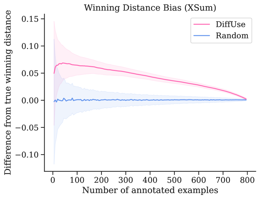
Figure 5: Deviation from test winning distance. The figure depicts the difference between the estimated winning distance and the test winning distance, aggregated across all model pairs over XSum. Shaded areas denote standard error (averaged across pairs). Clearly, our method favors the test winning model, providing a biased estimate in its favor. The bias dissipates as more examples are selected, only converging to the true distance for the full set of examples.

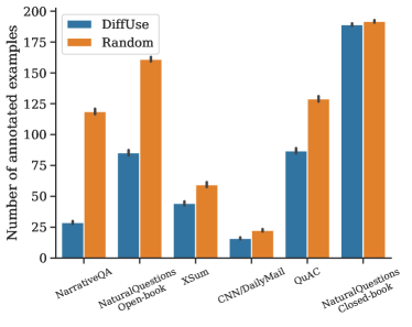
(a)

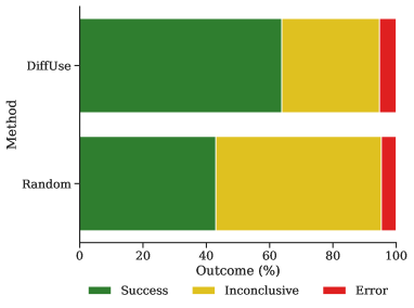
(b)

Figure 6: Iterative selection results. The plots depict the results of applying iterative selection (Algorithm 1; with $p=0.2$, $n=5$, and $b=200$), comparing DiffUse to random sampling. Results are aggregated across $666$ model pairs. The left panel depicts the mean number of examples annotated by the oracle before reaching the stopping criterion. The right panel depicts the proportion of outcomes of the iterative selection experiments – i.e., was a winning model determined, and was this decision correct – aggregated across all datasets. See also App. Table 2, 3.

6.2 Practical Iterative Selection Algorithm

Accuracy in estimating the winning model can vary widely, depending on the number of examples as well as the actual performance gap (Fig. 3). In a practical scenario, however, users presumably do not know in advance the size of the performance gap between the models they compare; moreover, after annotating some examples with the oracle and estimating the winning model, users will not know whether the estimation is in fact correct.

Thus, in order to apply oracle effort minimization strategies in practice, there is a need for a practical approach that determines the required number of examples dynamically, and provides some approximation of the reliability of the estimate.

To this end, we propose an iterative method for selecting examples. In this approach, the number of examples sent to the oracle is increased gradually, until a predefined reliability-oriented threshold is met. Hierarchical clustering naturally lends itself to an iterative solution: suppose we have clustered the difference vectors into $N$ clusters, and the oracle has annotated the $N$ selected examples, yet we suspect that the preference estimation is not sufficiently reliable. In this case, we can now cluster the vectors into $k+1$ clusters; this will further partition one of the previous clusters, providing two new examples to be labeled by the oracle. With each partitioning step, the amount of information increases, and this procedure is repeated until reaching the threshold/stopping criterion.

The full iterative selection flow is described in Algorithm 1. For the stopping criterion, we propose to use a reliability threshold based on the hypergeometric distribution (see Appendix A.2 for details). The threshold is a heuristic that approximates the level of risk, where a chosen threshold of $0.1$, for example, loosely corresponds to a likelihood of up to $10\%$ of choosing the wrong model. The risk threshold is set in advance, and reflects a preferred point on a trade-off: between the user’s tolerance for error, and the amount of examples the oracle will need to annotate.

Results for the iterative algorithm are shown in Figure 6. Clearly, DiffUse provides a significant advantage over random selection, increasing the likelihood of successfully determining the winner (right panel), while significantly reducing the number of examples sent to the oracle (left panel).

Note that the number of annotations in practice varies widely, and is linked to the performance gap between the models. For instance, in the Closed-Book version of NaturalQuestions, a large number of examples is annotated, and the outcome is usually inconclusive (left panel of Fig. 6, App. Tab. 2); this is because the distances between models in this dataset are quite small (cf. Fig. 2), making it difficult to conclusively determine the winner.

7 Analysis

7.1 Method Parameters

Next, we examine $3$ choices in the flow of DiffUse (Fig. 1): the representations of examples, the clustering algorithm and the cluster representative selection.

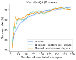
(a)

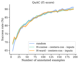
(b)

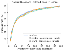
(c)

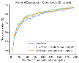
(d)

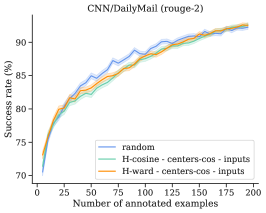
(e)

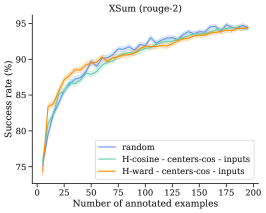
(f)

Figure 14: Input-based clustering results. Plots depict success rates of model preference estimation, aggregated over $666$ unique model pairs. Each panel depicts a different dataset.

Our method relies on difference vectors (i.e., subtraction of output embeddings) to represent examples. A naive approach would be to cluster the embeddings of inputs, akin to some methods in active learning (Zhang et al., 2022). However, we find that this approach does not consistently outperform random sampling (App. Figure 14). We also compare various approaches for aggregating the semantic embeddings of the two outputs. We find that using difference vectors, i.e., subtracting the two embeddings, outperfoms other aggregation methods, such as concatenation or addition.

In contrast, we find that the choices of clustering algorithm and representative selection are less significant, and performance differences are not dramatic (Appendix A.3). Note that all configurations significantly outperform the random baseline.

7.2 Which examples are selected?

As shown above, the success of our method hinges on the use of output difference vectors. Next, we perform several analyses to better understand how clustering these vectors enables selecting examples that are informative for the oracle.

The difference vectors represent variance in the outputs, and thus in the models’ behavior for a given task. Assuming an ideal semantic encoder, highly distinct outputs should yield difference vectors with high norms, signifying pronounced dissimilarities. Conversely, similar outputs would result in lower norms, indicating subtle differences.

7.2.1 Cluster Sizes and Difference Norms

Since the distance between two vectors is bounded by the sum of their norms, difference vectors with smaller norms have a higher tendency to be clustered together. This is nicely demonstrated in Figure 7, which depicts an example two-dimensional projection of difference vectors for a pair of models. The projection reveals a densely populated region close to zero, corresponding to cases where the model outputs show more subtle differences.

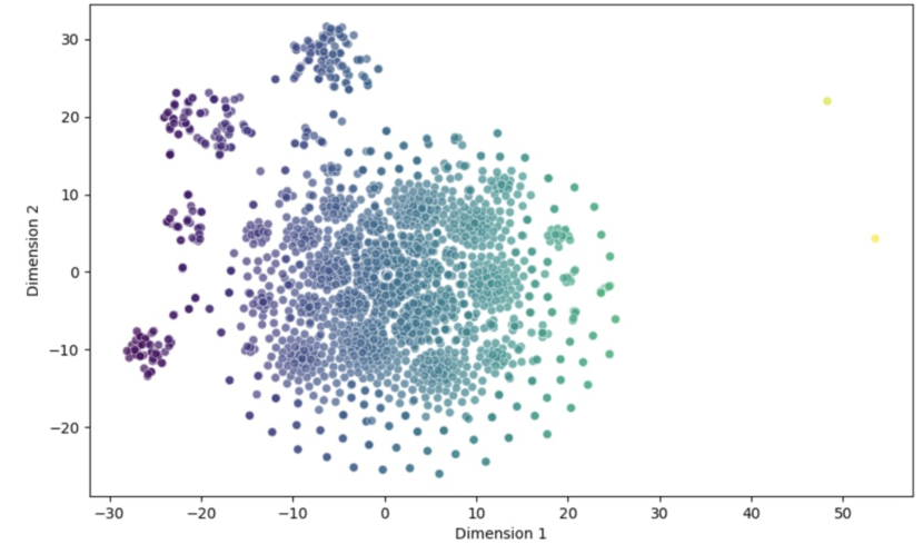
Figure 7: Example 2-D projection. A t-SNE (van der Maaten and Hinton, 2008) projection of the difference vectors from a randomly selected pair of models in XSum. The observed behavior, where most vectors are centered around zero, and the distribution is sparser away from it, is consistent across model pairs.

Figure 8 illustrates the relation between the sizes of clusters and the average norm of difference vectors within the cluster. Evidently, clustering the difference vectors tends to result in a small number of large clusters, which have a low average norm (bottom-right area of Fig. 8), alongside a large number of small clusters with higher norm values. Often, over half of the vectors are assigned to a single cluster with small norms. As DiffUse selects one example from each cluster, the sub-population of examples with small difference norms is under-represented in the set of selected examples.

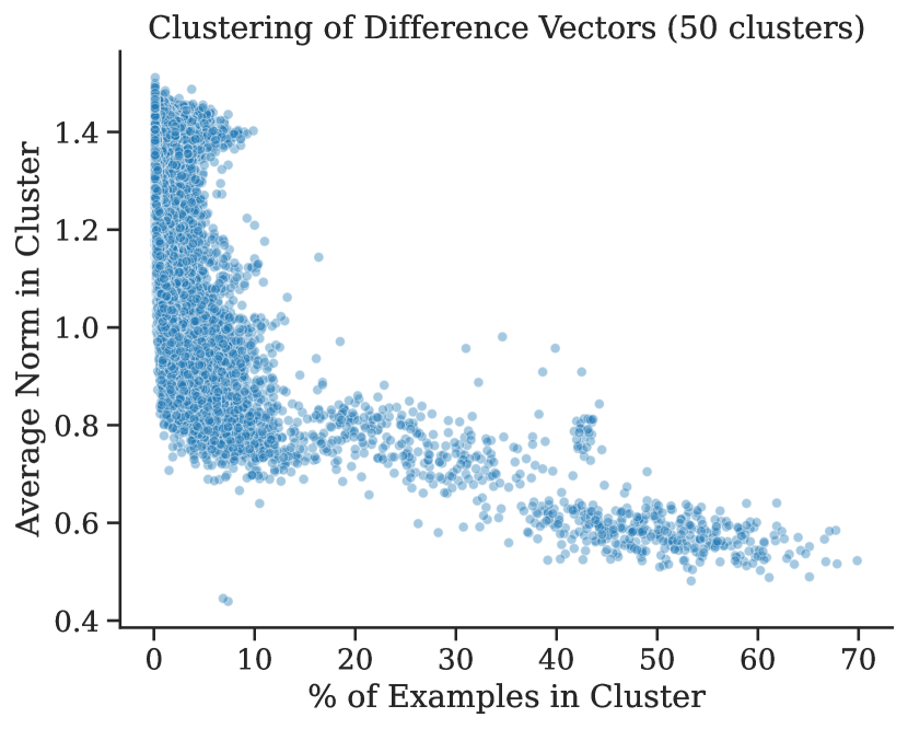
Figure 8: Cluster size vs. average vector norm. Hierarchical clustering results of the difference vectors, for the XSum dataset when partitioning into $50$ clusters. Each point represents a single cluster; in total, the plot depicts $\sim 33$K points ($666$ model pairs $\times~{}50$ resulting clusters per pair). The x-axis reflects the percentage of all examples that are in the cluster, and the y-axis is the average vector norm within the cluster. Results are characterized by a few very large clusters with a small average norm (bottom right); this pattern is consistent across different numbers of clusters (App. Fig. 15)

Figure 9 directly depicts the norm size distribution of the selected examples. Again, we see that DiffUse is biased toward high-norm instances.

7.2.2 Norms and Winning Model

We have demonstrated that our method over-represents difference vectors with a higher norm. This leads to the question of how this tendency relates to model preference.

Figure 10 depicts the relation between the norm of difference vectors and estimation of the test winning model. As can be seen, the preference label of instances with higher difference norms is more likely to align with the test winning model. This is in line with the winner-bias shown in Fig. 5.

A possible explanation for this observation is that larger semantic differences between the models’ outputs are expected be associated with larger quality gaps; meanwhile, the chances that the weaker model will beat the stronger model’s output by a large margin are low. Thus, the lower the difference norm, the higher the probability of the preference label to be “erroneous”, namely for the weaker model to be preferred by the oracle.

Given the informativeness of high-norm output pairs, a simple approach would be to forgo clustering, and simply select the instances with the highest norm for annotation. However, this results in inferior performance (Appendix A.4). This is not surprising; selecting by norm alone can result in outliers, and may not be representative of the space of difference vectors.

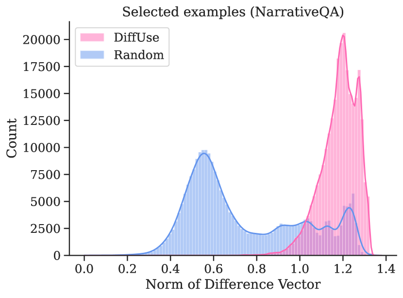
Figure 9: Norm size distribution of examples. These histograms depict the norm of difference vectors for the output pairs selected for annotation (across all NarrativeQA selection runs). Compared to random sampling, DiffUse selects examples with higher vector norms.

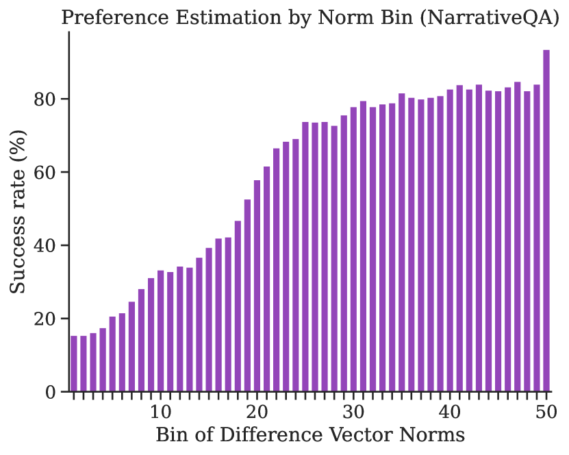
Figure 10: Norms and preference estimation. The plot depicts the success rate at estimating the better of two models, based on sub-populations with varying vector norms. For each model pair, the difference vectors were partitioned based on their norm sizes into $50$ equal-count bins, and each bin of instances was used to estimate the test winning model. The plot presents an aggregation across all model pairs over NarrativeQA.

To sum, clustering difference vectors over-represents output pairs with a large norm (§7.2.1). These, in turn, are more strongly associated with the overall winning model (§7.2.2). Thus, our analyses illustrate how DiffUse is able to correctly determine the winning model using fewer annotations.

8 Related Work

In light of the soaring costs of language model evaluation, even when using automatic metrics, some recent works (Perlitz et al., 2023a; Maynez et al., 2023) have studied the effects of reducing the size of evaluation sets – via random sampling – on the reliable ranking of models.

Other prior works have examined methods of intelligently selecting subsets of examples for evaluation, aiming to find sets of examples that are more informative than randomly sampled instances.

Rodriguez et al. (2021); Vania et al. (2021) look at the problem of selecting examples for evaluating new models, given fully-annotated question answering data for an existing set of models. They show that some selection strategies, based on item response theory (Lord et al., 1968), outperform the random selection baseline for ranking new models on a question answering task.

Several works have addressed label-efficient assessment in the context of classifier performance. Katariya et al. (2012) propose a label-efficient algorithm to gain better accuracy estimates of classifiers, by selecting examples to label based on stratified sampling. Ji et al. (2021) suggest an active Bayesian approach that uses inferred uncertainty to guide selection of instances. Inspired by works on active learning, Kossen et al. (2021) propose methods based on a stochastic acquisition process, to avoid unwanted and highly problematic biases involved in active selection of test set examples. They show the effectiveness of their acquisition functions on both classification and regression models. Ha et al. (2021) suggest an iterative method that utilizes a surrogate model to estimate the metrics of interest over the unlabeled test set, and labels examples that lead to maximal uncertainty reduction of the metric estimation. With a similar spirit to our work, Vivek et al. (2023) find anchor examples in classification datasets that represent how confident different models are over those input examples.

Our work differs from these prior efforts in that we tailor our approach to the nature of text generation, do not assume a “train set” of model annotations, and focus on making an informed preference decision between two candidate models.

The current work also draws inspiration from works finding patterns in model behaviour, for instance that models seem to learn in a similar order and make the same mistakes (Choshen et al., 2022; Hacohen et al., 2020), and that evaluation trained on one model can work well over another (Wan et al., 2022) or even work on the input level alone (Don-Yehiya et al., 2022). More closely, our work relates to efforts aimed at reducing annotation costs during training, namely iterative active learning approaches (Zhang et al., 2022; Ein-Dor et al., 2020a; Perlitz et al., 2023b).

9 Discussion

We have shown that our method, DiffUse, provides significant cost savings in obtaining preference judgements from an oracle. Using a dynamic algorithm such as the one proposed here (§6.2), practitioners can obtain a minimal number of judgements while maintaining high evaluation reliability.

In this work we provide a somewhat novel view into the notion of bias. Bias in an example selection method is often seen as a problem, one that should be avoided or corrected (Kossen et al., 2021). In contrast, in our setting the power of DiffUse is precisely the fact that it is biased in a very particular direction (Fig. 5, §7.2), reducing the likelihood for error in the context of binary preference decisions.

Here we examined the problem of selecting between a pair of candidate models. We leave to future work the scenario of picking from a larger set of candidates. This may entail adapting our method to a multi-model scenario, or combining our pairwise approach with an efficient method for limiting the number of pairwise comparisons (e.g., Mohankumar and Khapra, 2022).

While the current work deals with model selection, our approach of modeling differences between outputs can potentially be applicable for other purposes as well. This can include qualitative assessment of model behaviours, collection of preference data for training reward models, and more.

Limitations

As our approach relies on obtaining representations of model outputs, it incurs the non-trivial computational cost of performing inference over the set of examples to be clustered, in the range of hundreds of examples. Thus, our method is only suited for the (very common) scenario where the cost of applying the oracle is significantly greater than the cost of performing inference on a somewhat larger set of examples. This is the case for example when the oracle is a paid API or a human annotator.

As noted in §6.1, DiffUse is a biased approach that tends to over-represent subpopulations of the of examples. Here we show empirically – across model pairs and across datasets – that this method provides significant and consistent gains in relation to random selection. However, as also mentioned in App. A.2, for a given attempt at model comparison there is no theoretical or statistical guarantee of the probability of making the correct choice.

Our study is motivated by the fact that obtaining a large amount of human quality or preference judgments for a target generation task and set of models is prohibitively expensive. Ironically, this also means it is not trivial to obtain large-scale manually annotated data that can be used for evaluating the accuracy of our oracle minimization approach (existing preference datasets, e.g. for RLHF, are extremely diverse and do not have a well-defined notion of target tasks). Hence, here we rely on the automated metrics in HELM to simulate different types of oracles. This is a limitation of our experiments as we do not directly demonstrate our method on expensive real-world oracles.

Appendix A Appendix

Task	Scenario	Description
Question Answering	NarrativeQA	The NarrativeQA benchmark for reading comprehension over narratives Kočiský et al. (2018)
	NaturalQuestions (closed-book)	The NaturalQuestions Kwiatkowski et al. (2019) benchmark for question answering based on naturally-occurring queries through Google Search. The input does not include the Wikipedia page with the answer.
	NaturalQuestions (open-book)	The NaturalQuestions Kwiatkowski et al. (2019) benchmark for question answering based on naturally-occurring queries through Google Search. The input includes the Wikipedia page with the answer.
	QuAC (Question Answering in Context)	The QuAC benchmark for question answering in the context of dialogues Choi et al. (2018).
Summarization	XSUM	The XSUM benchmark for text summarization of BBC news articles Narayan et al. (2018)
	CNN/DailyMail	The CNN/DailyMail benchmark for text summarization Nallapati et al. (2016).

Table 1: The HELM scenarios we used for our experiments, which include short and long text output tasks.

A.1 Full Results

Results for the $6$ text generation scenarios (datasets) in HELM, with $3$ different metrics for each scenario, are presented in Figure 11.

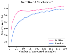
(a)

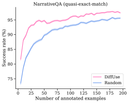
(b)

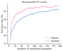
(c)

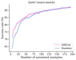
(d)

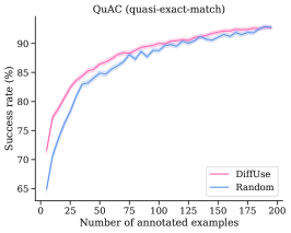
(e)

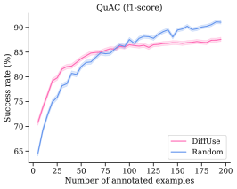
(f)

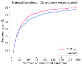
(g)

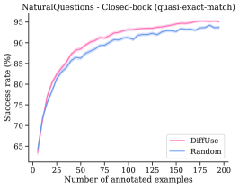
(h)

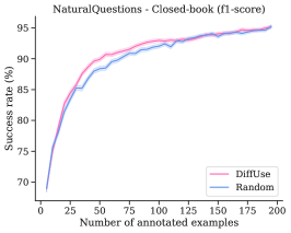
(i)

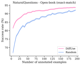
(j)

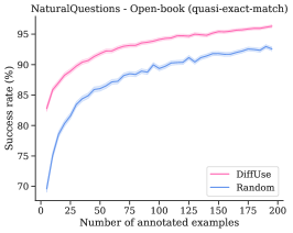
(k)

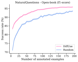
(l)

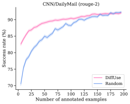
(m)

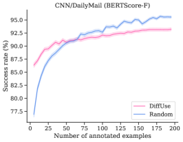
(n)

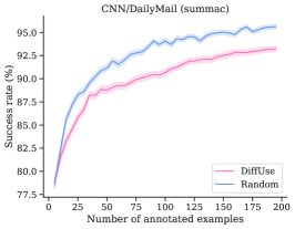
(o)

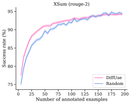
(p)

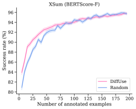
(q)

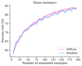
(r)

Figure 11: Full results. Plots depict success rates of model preference estimation, aggregated over $666$ unique model pairs. Each panel depicts a different combination of dataset and "oracle" (reference-based evaluation metric).

A.2 Iterative Selection Threshold

As described in §6.2 and Algorithm 1, we propose an iterative algorithm for annotating examples by the oracle and choosing the winning model.

We opt for a reliability-oriented stopping criterion that is based on the hypergeometric distribution. This distribution describes the probability of ‘success’ when sampling without replacement, and is parameterized by a population size $N$, sample size $n$, number of successes in the population $K$ and number of successes in the sample $k$.

Specifically, we look at the hypergeometric distribution survival function, $sf_{hypergeom}(k-1)$, which describes the probability of getting $k$ or more successes by chance. In a model comparison scenario, $n$ corresponds to the number of examples annotated by the oracle, and $k$ to the number of votes received by the winning model within this set. We define the null hypothesis as one where the winning model is the winner in $50\%$ of the instances in the full test set, i.e., where $K=N/2$. Using this value for $K$, The result $sf(k-1)$ thus reflects how likely or unlikely it is to get a value of $k$ or higher given a ground-truth $50\%$ win rate.

For instance, say we select examples out of a pool of $500$ unlabeled examples. The oracle is given a total of $10$ examples to label, and determines that model $A$ was the winner in $8$ of them:

$$sf(k-1,N,K,n)=sf(7,500,250,10)=0.0529$$

Thus, in this example – given the null hypothesis and assuming a hypergeometric distribution – there is only a $\approx{5\%}$ probability of getting such a high win rate – or a higher one – by chance. In other words, a situation where model $A$ is the winner in just $50\%$ of the full test set, and an $8/10$ result was obtained, is relatively unlikely. A situation where model $A$ is the winner in under $50\%$ of the test set is even less likely. This means that the user can be fairly confident that the correct winner was chosen.

Thus, when applying the iterative algorithm, the user sets an acceptable risk level – say, 10% – in advance; at each iteration, $sf$ is calculated using the current values of $n$ and $k$; if the value of $sf$ is lower than the risk level, the result is considered sufficiently reliable; if not, the sample size $n$ is increased and additional examples are labeled.

Note that we use this probability-based threshold merely as a heuristic, or proxy, for the real probability. In practice, the assumptions of the hypergeometric distribution are violated in our case. Most importantly, this distribution describes random selection, whereas DiffUse is non-random, and in fact has a distinct bias towards selecting certain kinds of examples (§6.1, §7). Moreover, even for random selection, the approach does not precisely match the model comparison setting; for instance, if there is a large number of examples where there is a tie between the two models, a null hypothesis of a $50\%$ win-rate is in fact overly conservative. Thus, while the threshold chosen by the user serves as a good proxy for the estimated error rate, and is thus suitable as a stopping criterion, it does not guarantee the actual error rate value. In our empirical experiments, for all datasets the error rate was lower than the chosen risk threshold (cf. Tables 2,3).

When opting for higher risk thresholds, there is a large impact to the initial number of labeled examples, because wins that are based on a very small sample (e.g., $3$ out of $3$) are avoided, even though they may meet the risk threshold.

		# Annotations $\downarrow$	Error (%) $\downarrow$	Success (%) $\uparrow$	Inconclusive (%) $\downarrow$	Average Distance	Avg. Dist.	Avg. Dist.	Avg. Dist.
Dataset	Method						(Error) $\downarrow$	(Success)	(Inconcl.) $\downarrow$
CNN/DailyMail	DiffUse	15.90	11.97	86.50	1.53	0.27	0.06	0.30	0.09
	Random	22.47	16.77	80.32	2.91	0.27	0.10	0.31	0.07
NarrativeQA	DiffUse	28.77	4.20	89.64	6.16	0.31	0.06	0.34	0.05
	Random	118.69	0.72	43.03	56.25	0.31	0.11	0.55	0.13
NaturalQuestions Closed-book	DiffUse	189.05	0.20	6.40	93.41	0.15	0.12	0.32	0.13
	Random	191.74	0.11	4.37	95.53	0.15	0.10	0.32	0.14
NaturalQuestions Open-book	DiffUse	85.25	0.93	62.81	36.26	0.20	0.03	0.28	0.06
	Random	160.97	0.17	21.79	78.05	0.20	0.15	0.44	0.13
QuAC	DiffUse	86.91	7.75	58.24	34.01	0.15	0.07	0.20	0.08
	Random	128.93	4.37	35.93	59.70	0.15	0.09	0.25	0.10
XSum	DiffUse	44.25	6.86	79.38	13.75	0.30	0.09	0.35	0.08
	Random	59.39	6.05	72.45	21.50	0.30	0.10	0.37	0.09

Table 2: Iterative selection results ($p=0.2$). The table depicts the results of applying iterative selection (Algorithm 1; with $p=0.2$, $n=5$, and $b=200$), comparing DiffUse to random sampling. Results are aggregated across $666$ model pairs. The table details the amount of annotations performed before reaching the stopping criterion, and the outcomes of the selection experiments (Success/Error/Inconclusive). In addition, it details the average winning distance (§3) between model pairs, broken down by the experiment outcomes. $\downarrow$: Lower is better.
Where the experiment result is inconclusive or the wrong winning model is chosen, the performance gap between models is quite small; Thus, even where the user is unable to correctly determine the better-performing model, the cost of this failure is relatively limited.

		# Annotations $\downarrow$	Error (%) $\downarrow$	Success (%) $\uparrow$	Inconclusive (%) $\downarrow$	Average Distance	Avg. Dist.	Avg. Dist.	Avg. Dist.
Dataset	Method						(Error) $\downarrow$	(Success)	(Inconcl.) $\downarrow$
CNN/DailyMail	DiffUse	34.54	7.13	86.44	6.43	0.27	0.05	0.30	0.07
	Random	51.98	8.65	79.32	12.03	0.27	0.07	0.32	0.07
NarrativeQA	DiffUse	47.80	1.35	84.53	14.11	0.31	0.05	0.36	0.05
	Random	132.75	0.05	37.69	62.27	0.31	0.05	0.59	0.14
NaturalQuestions Closed-book	DiffUse	195.37	0.00	3.30	96.70	0.15	NaN	0.37	0.14
	Random	197.35	0.00	1.65	98.35	0.15	NaN	0.40	0.14
NaturalQuestions Open-book	DiffUse	111.02	0.23	52.87	46.91	0.20	0.02	0.30	0.07
	Random	172.34	0.02	16.71	83.27	0.20	0.05	0.49	0.14
QuAC	DiffUse	129.20	2.96	43.26	53.78	0.15	0.06	0.23	0.09
	Random	158.26	1.14	25.11	73.75	0.15	0.08	0.29	0.11
XSum	DiffUse	71.18	2.16	73.21	24.62	0.30	0.07	0.37	0.08
	Random	88.84	2.09	63.90	34.01	0.30	0.08	0.41	0.10

Table 3: Iterative selection results ($p=0.1$). The table depicts the results of applying iterative selection (Algorithm 1; with $p=0.1$, $n=5$, and $b=200$), comparing DiffUse to random sampling. Results are aggregated across $666$ model pairs. The table details the amount of annotations performed before reaching the stopping criterion, and the outcomes of the selection experiments (Success/Error/Inconclusive). In addition, it details the average winning distance (§3) between model pairs, broken down by the experiment outcomes. $\downarrow$: Lower is better.
Where the experiment result is inconclusive or the wrong winning model is chosen, the performance gap between models is quite small; Thus, even where the user is unable to correctly determine the better-performing model, the cost of this failure is relatively limited.

A.3 Clustering Methods and Representative Selection

We conducted selection experiments employing various clustering algorithms. We found that the majority of these algorithms produced results that exceeded those of random sampling.

Below, we provide details regarding the clustering methods we explored:

1. Hierarchical Clustering

   1. Euclidean Distance: Hierarchical clustering with Euclidean distance measures dissimilarity between data points based on their spatial coordinates. It facilitates cluster creation by iteratively merging data points to minimize within-cluster variance.

   2. Cosine Distance: Hierarchical clustering using cosine distance measures similarity between data points via the cosine of the angle between vectors. Cosine distances were employed during the merging process.

2. K-Means Clustering: K-Means clustering partitions data into ’k’ clusters by iteratively assigning data points to the nearest cluster center and updating centers based on the mean of assigned points. Our approach incorporated "greedy k-means++" for centroid initialization, leveraging an empirical probability distribution of points’ contributions to overall inertia.

The model preference success rates for different clustering algorithms, selecting a single representative from each cluster based on distance to the cluster center, are shown in Figure 12.

We also explored various methods for selecting a representative from each cluster. These methods encompassed random selection, choosing the example nearest to the centroid (employing either Euclidean or cosine distances), and selecting the example with the maximum norm. As seen in Figure 13, the choice of representatives did not significantly impact the outcomes.

Here we focus on clustering algorithms as the approach for sampling from the vector distribution. However, other selection approaches, such as core-set (Sener and Savarese, 2018) or IDDS (Tsvigun et al., 2022), may also prove effective.

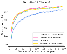
(a)

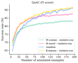
(b)

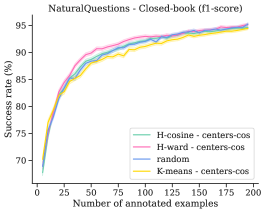
(c)

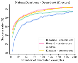
(d)

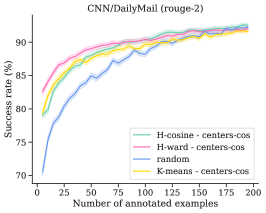
(e)

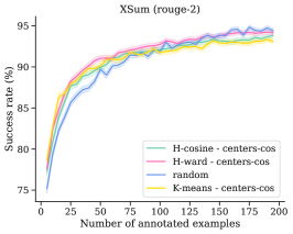
(f)

Figure 12: Comparing clustering algorithms. Plots depict success rates of model preference estimation, aggregated over $666$ unique model pairs. Each panel depicts a different dataset. For all clustering methods, a single example – closest in cosine distance to the cluster center – is selected from each cluster.

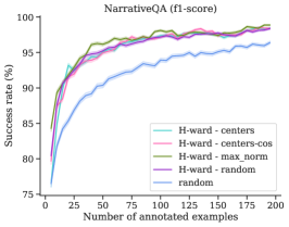
(a)

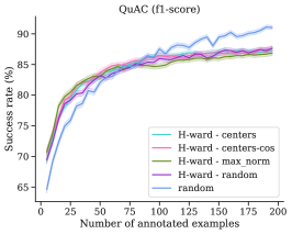
(b)

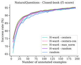
(c)

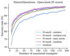
(d)

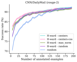
(e)

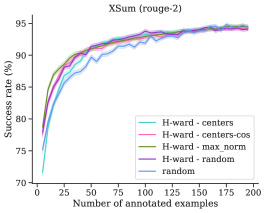
(f)

Figure 13: Comparing representative selection methods. Plots depict success rates of model preference estimation, aggregated over $666$ unique model pairs. Each panel depicts a different dataset. For all non-random methods, hierarchical clustering with Ward linkage was used to partition the difference vectors; the plots compare approaches for selecting a single representative from each cluster.

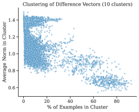
(a)

(b)

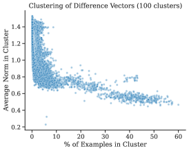
(c)

Figure 15: Cluster size vs. average vector norm. The plot describes the results of hierarchical clustering of the difference vectors, for the XSum dataset when partitioning into different numbers of clusters. Each point represents a single cluster; in total, each panel depicts between $6.7$K and $67$K points ($666$ model pairs $\times$ the number of clusters per pair). The x-axis reflects the percentage of all examples that are in the cluster, and the y-axis is the average vector norm within the cluster. The results are characterized by very large clusters with a small average norm (bottom right of the plots).

A.4 Norm of Difference Vectors

We explored the norm of the difference vectors as a signal for selecting examples. While we experimented with various binning scenarios, the best outcomes were obtained by directly selecting the vectors with the maximal norm. However, even this approach proved inconsistent across datasets and tasks, as demonstrated in Fig. 16. This is not surprising; selecting by norm alone can result in outliers, and may not be representative of the space of difference vectors.

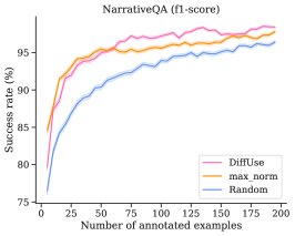
(a)

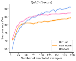
(b)

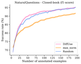
(c)

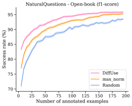
(d)

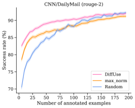
(e)

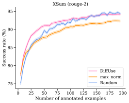
(f)

Figure 16: Max-norm baseline results. Plots depict success rates of model preference estimation, aggregated over $666$ unique model pairs. Each panel depicts a different dataset.

References

- Biderman et al. (2023) Stella Biderman, USVSN Sai Prashanth, Lintang Sutawika, Hailey Schoelkopf, Quentin Anthony, Shivanshu Purohit, and Edward Raf. 2023. Emergent and predictable memorization in large language models. arXiv:2304.11158.
- Callison-Burch et al. (2007) Chris Callison-Burch, Cameron Fordyce, Philipp Koehn, Christof Monz, and Josh Schroeder. 2007. (meta-) evaluation of machine translation. In Proceedings of the Second Workshop on Statistical Machine Translation, pages 136–158, Prague, Czech Republic. Association for Computational Linguistics.
- Celikyilmaz et al. (2020) Asli Celikyilmaz, Elizabeth Clark, and Jianfeng Gao. 2020. Evaluation of text generation: A survey. arXiv:2006.14799.
- Choi et al. (2018) Eunsol Choi, He He, Mohit Iyyer, Mark Yatskar, Wen-tau Yih, Yejin Choi, Percy Liang, and Luke Zettlemoyer. 2018. QuAC: Question answering in context. In Proceedings of the 2018 Conference on Empirical Methods in Natural Language Processing, pages 2174–2184, Brussels, Belgium. Association for Computational Linguistics.
- Choshen et al. (2022) Leshem Choshen, Guy Hacohen, Daphna Weinshall, and Omri Abend. 2022. The grammar-learning trajectories of neural language models. In Proceedings of the 60th Annual Meeting of the Association for Computational Linguistics (Volume 1: Long Papers), pages 8281–8297.
- Don-Yehiya et al. (2022) Shachar Don-Yehiya, Leshem Choshen, and Omri Abend. 2022. PreQuEL: Quality estimation of machine translation outputs in advance. In Proceedings of the 2022 Conference on Empirical Methods in Natural Language Processing, pages 11170–11183, Abu Dhabi, United Arab Emirates. Association for Computational Linguistics.
- Ein-Dor et al. (2020a) Liat Ein-Dor, Alon Halfon, Ariel Gera, Eyal Shnarch, Lena Dankin, Leshem Choshen, Marina Danilevsky, Ranit Aharonov, Yoav Katz, and Noam Slonim. 2020a. Active Learning for BERT: An Empirical Study. In Proceedings of the 2020 Conference on Empirical Methods in Natural Language Processing (EMNLP), pages 7949–7962, Online. Association for Computational Linguistics.
- Ein-Dor et al. (2020b) Liat Ein-Dor, Eyal Shnarch, Lena Dankin, Alon Halfon, Benjamin Sznajder, Ariel Gera, Carlos Alzate, Martin Gleize, Leshem Choshen, Yufang Hou, et al. 2020b. Corpus wide argument mining—a working solution. In Proceedings of the AAAI Conference on Artificial Intelligence, volume 34, pages 7683–7691.
- Ha et al. (2021) Huong Ha, Sunil Gupta, Santu Rana, and Svetha Venkatesh. 2021. ALT-MAS: A data-efficient framework for active testing of machine learning algorithms. arXiv:2104.04999.
- Hacohen et al. (2020) Guy Hacohen, Leshem Choshen, and Daphna Weinshall. 2020. Let’s agree to agree: Neural networks share classification order on real datasets. In International Conference on Machine Learning, pages 3950–3960. PMLR.
- Ji et al. (2021) Disi Ji, Robert L. Logan, Padhraic Smyth, and Mark Steyvers. 2021. Active bayesian assessment of black-box classifiers. Proceedings of the AAAI Conference on Artificial Intelligence, 35(9):7935–7944.
- Katariya et al. (2012) Namit Katariya, Arun Iyer, and Sunita Sarawagi. 2012. Active evaluation of classifiers on large datasets. In 2012 IEEE 12th International Conference on Data Mining, pages 329–338.
- Kočiský et al. (2018) Tomáš Kočiský, Jonathan Schwarz, Phil Blunsom, Chris Dyer, Karl Moritz Hermann, Gábor Melis, and Edward Grefenstette. 2018. The NarrativeQA reading comprehension challenge. Transactions of the Association for Computational Linguistics, 6:317–328.
- Kossen et al. (2021) Jannik Kossen, Sebastian Farquhar, Yarin Gal, and Tom Rainforth. 2021. Active testing: Sample-efficient model evaluation. In Proceedings of the 38th International Conference on Machine Learning, volume 139 of Proceedings of Machine Learning Research, pages 5753–5763. PMLR.
- Kwiatkowski et al. (2019) Tom Kwiatkowski, Jennimaria Palomaki, Olivia Redfield, Michael Collins, Ankur Parikh, Chris Alberti, Danielle Epstein, Illia Polosukhin, Jacob Devlin, Kenton Lee, Kristina Toutanova, Llion Jones, Matthew Kelcey, Ming-Wei Chang, Andrew M. Dai, Jakob Uszkoreit, Quoc Le, and Slav Petrov. 2019. Natural questions: A benchmark for question answering research. Transactions of the Association for Computational Linguistics, 7:452–466.
- Li et al. (2019) Margaret Li, Jason Weston, and Stephen Roller. 2019. Acute-eval: Improved dialogue evaluation with optimized questions and multi-turn comparisons. arXiv:1909.03087.
- Liang et al. (2022) Percy Liang, Rishi Bommasani, Tony Lee, Dimitris Tsipras, Dilara Soylu, Michihiro Yasunaga, Yian Zhang, Deepak Narayanan, Yuhuai Wu, Ananya Kumar, et al. 2022. Holistic evaluation of language models. arXiv:2211.09110.
- Liang et al. (2020) Weixin Liang, James Zou, and Zhou Yu. 2020. Beyond user self-reported Likert scale ratings: A comparison model for automatic dialog evaluation. In Proceedings of the 58th Annual Meeting of the Association for Computational Linguistics, pages 1363–1374, Online. Association for Computational Linguistics.
- Lord et al. (1968) FM Lord, MR Novick, and Allan Birnbaum. 1968. Statistical theories of mental test scores.
- Maynez et al. (2023) Joshua Maynez, Priyanka Agrawal, and Sebastian Gehrmann. 2023. Benchmarking large language model capabilities for conditional generation. In Proceedings of the 61st Annual Meeting of the Association for Computational Linguistics (Volume 1: Long Papers), pages 9194–9213, Toronto, Canada. Association for Computational Linguistics.
- Mohankumar and Khapra (2022) Akash Kumar Mohankumar and Mitesh Khapra. 2022. Active evaluation: Efficient NLG evaluation with few pairwise comparisons. In Proceedings of the 60th Annual Meeting of the Association for Computational Linguistics (Volume 1: Long Papers), pages 8761–8781, Dublin, Ireland. Association for Computational Linguistics.
- Müllner (2011) Daniel Müllner. 2011. Modern hierarchical, agglomerative clustering algorithms. arXiv:1109.2378.
- Nallapati et al. (2016) Ramesh Nallapati, Bowen Zhou, Cicero dos Santos, Çağlar Gulçehre, and Bing Xiang. 2016. Abstractive text summarization using sequence-to-sequence RNNs and beyond. In Proceedings of the 20th SIGNLL Conference on Computational Natural Language Learning, pages 280–290, Berlin, Germany. Association for Computational Linguistics.
- Narayan et al. (2018) Shashi Narayan, Shay B. Cohen, and Mirella Lapata. 2018. Don’t give me the details, just the summary! topic-aware convolutional neural networks for extreme summarization. In Proceedings of the 2018 Conference on Empirical Methods in Natural Language Processing, pages 1797–1807, Brussels, Belgium. Association for Computational Linguistics.
- Perlitz et al. (2023a) Yotam Perlitz, Elron Bandel, Ariel Gera, Ofir Arviv, Liat Ein-Dor, Eyal Shnarch, Noam Slonim, Michal Shmueli-Scheuer, and Leshem Choshen. 2023a. Efficient benchmarking (of language models). arXiv:2308.11696.
- Perlitz et al. (2023b) Yotam Perlitz, Ariel Gera, Michal Shmueli-Scheuer, Dafna Sheinwald, Noam Slonim, and Liat Ein-Dor. 2023b. Active learning for natural language generation. In Proceedings of the 2023 Conference on Empirical Methods in Natural Language Processing, pages 9862–9877, Singapore. Association for Computational Linguistics.
- Reimers and Gurevych (2019) Nils Reimers and Iryna Gurevych. 2019. Sentence-bert: Sentence embeddings using siamese bert-networks. In Conference on Empirical Methods in Natural Language Processing.
- Rodriguez et al. (2021) Pedro Rodriguez, Joe Barrow, Alexander Miserlis Hoyle, John P. Lalor, Robin Jia, and Jordan Boyd-Graber. 2021. Evaluation examples are not equally informative: How should that change NLP leaderboards? In Proceedings of the 59th Annual Meeting of the Association for Computational Linguistics and the 11th International Joint Conference on Natural Language Processing (Volume 1: Long Papers), pages 4486–4503, Online. Association for Computational Linguistics.
- Sedoc et al. (2019) João Sedoc, Daphne Ippolito, Arun Kirubarajan, Jai Thirani, Lyle Ungar, and Chris Callison-Burch. 2019. ChatEval: A tool for chatbot evaluation. In Proceedings of the 2019 Conference of the North American Chapter of the Association for Computational Linguistics (Demonstrations), pages 60–65, Minneapolis, Minnesota. Association for Computational Linguistics.
- Sener and Savarese (2018) Ozan Sener and Silvio Savarese. 2018. Active learning for convolutional neural networks: A core-set approach. In International Conference on Learning Representations.
- Tsvigun et al. (2022) Akim Tsvigun, Ivan Lysenko, Danila Sedashov, Ivan Lazichny, Eldar Damirov, Vladimir Karlov, Artemy Belousov, Leonid Sanochkin, Maxim Panov, Alexander Panchenko, Mikhail Burtsev, and Artem Shelmanov. 2022. Active learning for abstractive text summarization. In Findings of the Association for Computational Linguistics: EMNLP 2022, pages 5128–5152, Abu Dhabi, United Arab Emirates. Association for Computational Linguistics.
- van der Lee et al. (2021) Chris van der Lee, Albert Gatt, Emiel van Miltenburg, and Emiel Krahmer. 2021. Human evaluation of automatically generated text: Current trends and best practice guidelines. Computer Speech & Language, 67:101151.
- van der Lee et al. (2019) Chris van der Lee, Albert Gatt, Emiel van Miltenburg, Sander Wubben, and Emiel J. Krahmer. 2019. Best practices for the human evaluation of automatically generated text. In International Conference on Natural Language Generation.
- van der Maaten and Hinton (2008) Laurens van der Maaten and Geoffrey Hinton. 2008. Visualizing data using t-SNE. Journal of Machine Learning Research, 9(86):2579–2605.
- Vania et al. (2021) Clara Vania, Phu Mon Htut, William Huang, Dhara Mungra, Richard Yuanzhe Pang, Jason Phang, Haokun Liu, Kyunghyun Cho, and Samuel R. Bowman. 2021. Comparing test sets with item response theory. In Proceedings of the 59th Annual Meeting of the Association for Computational Linguistics and the 11th International Joint Conference on Natural Language Processing (Volume 1: Long Papers), pages 1141–1158, Online. Association for Computational Linguistics.
- Vivek et al. (2023) Rajan Vivek, Kawin Ethayarajh, Diyi Yang, and Douwe Kiela. 2023. Anchor points: Benchmarking models with much fewer examples. arXiv:2309.08638.
- Wan et al. (2022) Yu Wan, Dayiheng Liu, Baosong Yang, Haibo Zhang, Boxing Chen, Derek F Wong, and Lidia S Chao. 2022. Unite: Unified translation evaluation. arXiv preprint arXiv:2204.13346.
- Zhang et al. (2022) Zhisong Zhang, Emma Strubell, and Eduard Hovy. 2022. A survey of active learning for natural language processing. In Proceedings of the 2022 Conference on Empirical Methods in Natural Language Processing, pages 6166–6190, Abu Dhabi, United Arab Emirates. Association for Computational Linguistics.
- Zheng et al. (2023) Lianmin Zheng, Wei-Lin Chiang, Ying Sheng, Siyuan Zhuang, Zhanghao Wu, Yonghao Zhuang, Zi Lin, Zhuohan Li, Dacheng Li, Eric Xing, et al. 2023. Judging LLM-as-a-judge with MT-bench and chatbot arena. arXiv:2306.05685.