Stellar flares

Abstract

Magnetic storms on stars manifest as remarkable, randomly occurring changes of the luminosity over durations that are tiny in comparison to the normal evolution of stars. These stellar flares are bursts of electromagnetic radiation from X-ray to radio wavelengths, and they occur on most stars with outer convection zones. They are analogous to the events on the Sun known as solar flares, which impact our everyday life and modern technological society. Stellar flares, however, can attain much greater energies than those on the Sun. Despite this, we think that these phenomena are rather similar in origin to solar flares, which result from a catastrophic conversion of latent magnetic field energy into atmospheric heating within a region that is relatively small in comparison to normal stellar sizes. We review the last several decades of stellar flare research. We summarize multi-wavelength observational results and the associated thermal and nonthermal processes in flaring stellar atmospheres. Static and hydrodynamic models are reviewed with an emphasis on recent progress in radiation-hydrodynamics and the physical diagnostics in flare spectra. Thanks to their effects on the space weather of exoplanetary systems (and thus in our search for life elsewhere in the universe) and their preponderance in Kepler mission data, white-light stellar flares have re-emerged in the last decade as a widely-impactful area of study within astrophysics. Yet, there is still much we do not understand, both empirically and theoretically, about the spectrum of flare radiation, its origin, and its time evolution. We conclude with several big-picture questions that are fundamental in our pursuit toward a greater understanding of these enigmatic stellar phonemena and, by extension, those on the Sun.

1 Introduction

Stars produce energetic bursts of electromagnetic radiation that follows a sudden magnetic energy release into their atmospheres. These electromagnetic bursts are called flares, which occur on a very wide range of timescales, from seconds to days. Stellar flares are observed in all spectral windows, from the high-energy X-rays through the long wavelength radio waves. However, all wavelength regimes do not respond equally in energy and simultaneously in time. Some wavelengths (e.g., microwave) are dominated by nonthermal radiation, while others (optical, low-energy X-rays) are thought to result from primarily thermal radiative processes. The flare energy – both thermal and nonthermal – ultimately originates in the energy that is released from magnetic fields in stellar coronae. These magnetic fields, in turn, originate from turbulent convective energy transport and shear in rotating stellar envelopes, beneath the visible photosphere. The Sun is the best studied flare star due to its proximity to Earth and a fleet of multi-messenger instruments that continuously provide spatially resolved observations.

From Earth, solar and stellar flares are not detectable by the unaided human eye. Stars like the Sun, and other active stars like Algol that are visible to the naked eye, have too much background glare for our eyes to sense the flare brightness increases. In all-sky surveys that are sensitive to the apparent magnitudes of low-mass stars (fainter than a Johnson $V$-band magnitude of $\sim 9$), however, stellar flares are the most dramatic source of variability. By most dramatic, we mean that flares produce the largest changes in their apparent magnitudes per unit time when compared against nearly all other astrophysical phenomena.

In data from the upcoming Vera C. Rubin Observatory’s ten-year Legacy Survey of Space and Time (LSST), stellar flares will constitute a major source of variability [305]. Further, many of the largest events that are observed serendipitously (and those from very faint but populous low-mass stars) will be bona-fide transients, whereby the changes in brightness occur from sources that have not been detected in quiescence. Stellar flares are much shorter in duration and much less luminous than extra-galactic transient phenomena, such as supernovae, tidal disruption events, and optical counterparts to neutron star mergers. Most stellar flares can in principle be readily distinguished from these events given enough empirical information, despite some striking spectral similarities [124] in the optical spectra of kilonovae [669]. Due to their proximity to the solar system, the largest stellar flare events can trigger gamma ray observatories; these events are known as “superflares” in X-rays. Stellar superflares are factors of $\approx 10^{2}-10^{4}$ more energetic and luminous in comparison to the largest solar flares, which have bolometric energies of $E_{\rm{bol}}\approx 3-6\times 10^{32}$ erg [778, 779, 136, 306]. Such superflares were likely common when the Sun was very young and rotating much more rapidly than today [472]. Understanding the physical processes in stellar flares thus provides insight into the heliospheric conditions in the early history of our solar system [625].

It is timely for a review of recent observations and models of stellar flares. The next sunspot cycle maximum is approaching in late 2024 [727], and with it a deluge of flares and eruptions from the Sun. New and upcoming solar observatories, such as the Daniel K. Inouye Solar Observatory [628], the Expanded Owens Solar Valley Array [252], and the Interface Region Imaging Spectrograph [164], will provide new avenues for solar-stellar comparisons. The immaculate precision of Kepler [396], K2 [336], and the Transiting Exoplanet Survey Satellite [TESS; 627] observations has recently facilitated a resurgence in the study of optical broadband stellar flares. These missions provide access to stellar magnetic activity over long time baselines previously not feasible to observe from ground-based campaigns, and over a much larger variety of stars. Models of energy transport, atmospheric response, and emission line broadening have increased in accuracy and sophistication over a large range of heating parameters. As the community looks to next-generation modeling paths, analysis methods, and observational capabilities (such as new space missions and ground-based instruments), synthesizing recent findings and outstanding problems could help to steer these into productive directions. Additionally, stellar flare radiation is now considered an important factor in assessing exoplanet habitability and photochemistry [676, 666], and general interest within the solar and astrophysics communities has grown over the last decade.

1.1 Overview of this review

There have been several reviews on stellar flares prior to ca. 1990 [588, 106, 291]. The current review supplements these with results from the past three decades. This review features many results from flare studies of low-mass, M-dwarf (dM / MV) stars. Because of their low background glare from non-flaring regions, large contributions to Galactic populations, and inherently high flare rates, the M dwarfs tend to be the most commonly studied flare stars. Flares from active binary systems have also been very well-observed across the electromagnetic spectrum. Results from studies of post main-sequence single stars and young solar-type stars are covered as well. Surprisingly, certain wavelength regimes in M-dwarf flares have been more thoroughly observed than solar flares. Solar flares are not reviewed in any detail here, but a general overview is provided, since the interpretation of and modeling approach to stellar flares are dependent on knowledge of the particle acceleration, magnetic fields, and spatial resolution from the study of the Sun.

The primary purpose of this review is to serve as a compendium of references and to facilitate research in multi-wavelength observations and models of stellar flares. The target audience consists of beginning PhD students or interested scientists in other areas of astrophysics or solar physics. Every current topic in the study of stellar flares is not included here: for example, I leave all results from the TESS mission to the next iteration of this Living Review. Unfortunately, many important results and references cannot be discussed extensively in order to keep this review a reasonable length, while also allowing growth with future addenda. For the same reasons, every important result from the references cited herein regrettably cannot be included at this time. There are several comprehensive introductions to sub-topics in the stellar flare literature; these are indicated throughout instead of being repeated. Broader applications of flare research beyond stellar astrophysics (e.g., exoplanet habitability and exoplanet atmospheric photochemistry) are outside the scope of this review and are not covered. The study of stellar coronal mass ejections and their associated energetic particles is a vast and newly emerging field; these topics are only very briefly alluded to. This review focuses on the electromagnetic response of flaring stellar atmospheres and detailed modeling of the associated physical processes.

This review is organized as follows. We begin with a brief tour of the flare star next door, Proxima Centauri, which is about the same age as the Sun but is otherwise a much different star (Sect. 2). Then we take a detour for a brief introduction to solar flare terminology and phenomenology (Sect. 3). A general overview of all known types of stars that tend to flare is summarized in Sect. 4. The bulk of the review contains a synthesis of stellar flare observations across the electromagnetic spectrum with a focus on the near-ultraviolet (NUV) and optical response, which has not been the subject of most other reviews. Observational studies can be separated into two general topics: flare rates, which are primarily diagnosed through single-band photometry (Sect. 5), and multi-wavelength analyses, which are primarily accomplished through spectroscopy (Sect. 7). The final third of the review summarizes stellar flare modeling approaches (slab, semi-empirical, and radiative-hydrodynamic), beginning in Sect. 8. We go into detail in several areas within stellar flare modeling, focusing on key elements of radiation-hydrodynamics (Sect. 9) and the interpretation of chromospheric spectral line broadening in flares (Sect. 10). A comprehensive analysis of an “ideal” multi-wavelength data set is discussed in Sect. 11, and inferences of the stellar flare geometries are reviewed in Sect. 12. We conclude in Sect. 13 with six questions that we think are currently central in stellar flare research (excluding questions directly related to exoplanets). Throughout, we use the cgs (Gaussian) units system except for wavelengths in Å or in cases that are otherwise noted. In the appendices, we include a visual guide to common filters used in optical studies of stellar flares (Appendix A), some additional observational results from the literature are merged (Appendix B), several common slab modeling practices and assumptions are reviewed (Appendix C), and the basic microphysical processes that symmetrically broaden hydrogen lines in flares is summarized (Appendix D).

2 Our flare star neighbor: Proxima Centauri

The nearest star outside the solar system is Proxima Centauri, which is $\approx$1.3 parsecs, or 268,000 astronomical units (au), from the Earth, and is a low-mass ($\approx 0.12$ M_Sun) M dwarf star of spectral type M5.5Ve (dM5.5e) [299]. The hydrogen Balmer $\alpha$ line (6562.81 Å) is in emission (e) in quiescence outside of detectable flaring events, which occur very frequently. This star is a relatively old ($\approx 5-6$ Gyr) main sequence star, but it is still very magnetically active, consistent with the long magnetic activity lifetimes of low mass stars of its spectral type [769]. We describe some of the flare properties of this star from a night of monitoring during an observing run at La Silla Observatory in 2010, while also introducing basic point-source photometry measurements and terminology that are common to almost all analyses of flare star data.

A NUV light curve of Prox Cen [416] is shown in Fig. 1. The photometry was measured through a custom filter with a full-width-at-half-maximum (FWHM) of 100 Å centered at $\lambda_{\rm{cen}}=3500$ Å. This is a wavelength range over which the star has a very faint luminosity during non-flaring (“quiescent”, denoted by $q$) intervals. In less than seven hours of continuous 3 s exposures (and 1.5 s exposures at the end of the night), the star produced at least 16 flares at $>$3$\sigma$ (1$\sigma\approx 6$%) above the mean, which is indicated by a flux enhancement equal to 1.0 in the light curve. In quiescence, the star is very “red” since it has a very cool photospheric temperature ($<3000$ K), but the flare light causes the star’s total flux at Earth to become much “bluer”. In addition to the time-integrated flare energy (fluence), the peak flux enhancement is sometimes used to characterize the size of a flare. The peak magnitude change of a flare is related to the peak flux enhancement by

$$\Delta\mathrm{mag}_{\mathrm{peak}}=-2.5\ \mathrm{log}_{10}\ \left(C_{\mathrm{rel}}(t_{\mathrm{peak}})/C_{\mathrm{rel},q}\right)=-2.5\ \mathrm{log}_{10}\big{(}I_{f}(t_{\rm{peak}})+1\big{)}$$ (1)

where $C_{\rm{rel}}$ represents the measured counts per exposure through a bandpass and is calculated relative to the counts in that same exposure from a nearby comparison (non-variable) star or set of stars. The count flux enhancement, $C_{\rm{rel}}(t)/C_{\rm{rel},q}$, is normalized to a time interval over which the flare star is not clearly varying, usually taken right before a flare. The count flux enhancement has traditionally been denoted as $I_{f}+1$ [254]. Because the star is spatially unresolved, the values of $I_{f}(t)+1$ during a flare consist of the flux from the non-flaring regions on a flare star in addition to the flaring source; if the flare source has an optical thickness $\tau\gtrsim 1$ at wavelengths in this bandpass, then some or all of the pre-flare flux from the flare area may be diminished at time $t$ [298].

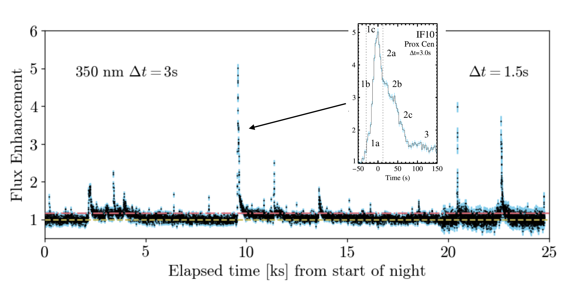
Figure 1: A light curve of Proxima Centauri in a narrowband (filter FWHM of 100 Å) centered in the near-ultraviolet, $U$-band wavelength regime. These data are from [416] and can be obtained from the Zenodo repository at https://doi.org/10.5281/zenodo.45878. The horizontal dashed lines indicate the mean flux enhancement (1.0) and $3\sigma$ above the mean (where $\sigma$ is the standard deviation outside of flaring). The inset shows the flare peaking at 2010 May 25 01:31:02 UT, which is referred to as the “IF10” event in [416]. The inset shows time relative to peak.

None of the flares in Fig. 1 are all that energetic. The flare with the largest peak flux enhancement of five would correspond to an energy of $3\times 10^{29}$ erg in the Johnson $U$ bandpass, which is traditionally the optimal broadband filter [$\lambda_{\rm{peak}}\sim 3700$ Å, a full-width-at-half maximum of $\sim 700$ Å; 506, 67] for stellar flare observations at ground-based observatories. This energy is nearly four times larger than the average $U$-band flare energy from Proxima Centauri [754] and a factor of 100 smaller than the largest event on the Sun that has been observed at similar wavelengths [539]. Multi-wavelength scaling relations [297, 422, 663, 562, 526, 136] facilitate comparison to the standard classification of solar flares according to their peak flux at Earth over the $\lambda=1-8$ Å band, as measured by the X-ray Sensor (XRS) on the Geostationary Operational Environmental Satellite (GOES). The A1.0, B1.0, C1.0, M1.0, and X1.0-class flares correspond to a range of peak X-ray irradiances logarithmically spanning $10^{-8}$ to $10^{-4}$ W m^-2, while those at $\geq 10^{-3}$ W m^-2 are sometimes clipped [339] and are given designations beginning with X10.0. The scaling relations imply that the large event on Proxima Centauri would correspond to approximately a GOES $1-8$ Å C-class flare if it had occurred on the Sun. However, Prox Cen occasionally erupts with energies that are comparable to, or even much greater than, typical GOES X-class flares from the Sun [283, 332]. Prox Cen also hosts a near Earth-mass planet at $\sim 0.05$ au [17], and unlike our relatively safe distance from solar flares at 1 au, equivalent flare energies from this star would bathe the surrounding planet in $400x$ the flux of high-energy radiations. Higher-mass, M3-M4 stars are known to emit even higher-energy flares than Prox Cen. For example, the most luminous event known resulted in a remarkably fast $\Delta t\approx 35$ s rise to a peak flux change of $\Delta V=-5$ mags ($L_{V,\rm{peak}}\approx 1.7\times 10^{32}$ erg s^-1) from a young M4$+$M4 binary DG CVn [108], for which the estimated values of the $U$-band energy and GOES class are $4.7\times 10^{34}$ erg and X600,000, respectively [571, 791]. [589] describes a remarkable EV Lac flare with a peak magnitude change in the $U$-band of $-7.2$ mags ($L_{U,\rm{peak}}=4.6\times 10^{31}$ erg s^-1) and a $U$-band energy of $7.23\times 10^{33}$ erg. [333] highlight several flares with extreme amplitudes ($\Delta g^{\prime}\leq-3$ mag) and energies ($E\approx 10^{35}-10^{36}$ erg) on M1-M4 stars in their optical survey.

The most common qualitative description of a flare light curve is a “FRED”: a fast-rise, exponential-decay. In Fig. 1, the flares exhibit a simple FRED shape at low time-resolution; however, at high-time resolution, much more variation in the temporal morphology is apparent, including two periods of the rise phase (1a, 1b), an extended peak (1c), two intervals of fast decay (2a, 2c), a stall between these two intervals (2b), and a gradual decay phase (3). These features are clear in some other events too [e.g., Figure 2 of 414, which is reproduced in the middle, right of Fig. 8 here], though the respective phases may have different durations, relative amplitudes, and integrated energies. High-time resolution observations of stellar flares were actually routine in the 1970s and 1980s using photometers, which have been superseded by high efficiency CCDs, culminating in the unprecedented precision from Kepler, K2, and TESS. The short timescale variations in stellar flares have actually long been recognized. The seminal study of [78] aptly summarized their findings as follows: “As the time resolution of observations has improved, the great complexity of the flare phenomenon has been revealed. The classical definition of a flare (i.e., rapid rise to maximum followed by a slower quasi-exponential decay) appears to be a gross oversimplification of the complex structures observed”.

3 Solar Flares and the Standard Flare Model

Only the very largest solar flare events could be detected in the optical if the Sun was at a similar distance as other stars. Recently, Kepler has provided the precision to detect a signal of $0.0170$%$-0.0270$% in optical enhancements that have been observed in Sun-as-a-star data [778, 422, 510] and from slowly rotating G dwarfs [472, 551, 555]. Nonetheless, it is generally thought that flares from other stars originate from the same or similar processes as solar flares. This is supported by the empirical Neupert effect [540], which was first reported in stellar flares in [298] and [280] (Sect. 7.7). In this section, we briefly review the standard solar flare model paradigm, whose phenomenology (e.g., footpoints, loops) and fundamental physical processes are widely adopted in the interpretation and analyses of stellar flares – either through direct application or through some sort of physical scaling to higher densities, magnetic fields, accelerated particle fluxes, etc… This section synthesizes decades of observations and theoretical work, and it presents our own (rather highly simplified) viewpoint of the entire process. Thus we give a non-exhaustive reference list. For more extensive reviews of solar flares, see [704], [342], [343], [62], [344], the entries within the Space Science Reviews Volume [166], the books by [23] and [706], and the review by [670]. For modern, comprehensive reviews of the observations and modeling of solar flares, see [232], [613], [387], and [388].

In the standard flare paradigm, magnetic potential energy is transferred to the atmosphere, which responds by radiating away this energy as the flare. There are generally two categories of solar flares [711, 385]. Mass and magnetic field are ejected away from the Sun during eruptive flares. In contrast, magnetized plasma is not ejected in confined, or compact, flares or the eruption may be undetectable. The collective process of the mass eruption and the electromagnetic flare is called a “solar eruptive event” (SEE). The left panel of Figure 2 illustrates the geometry of eruptive magnetic field above compact flare loops, with reconnection of magnetic fields in between [673]. This framework underlies most modern generalizations of flare-productive magnetic field topologies [e.g., Figure 1 of 386], which we now describe in further detail.

An SEE begins in active regions where there are colliding, non-conjugate sunspots of opposite polarity [128, 718, 623]. The demarcation that separates the bulk of the north and south polarities in an active region is termed the polarity inversion line (PIL). At the PIL, mixed negative and positive magnetic polarities appear as “salt-and-pepper” patterns in magnetograms where there is newly emerging magnetic flux. Ongoing magnetic flux emergence adds to a twisted, cool filament (flux rope) that is parallel to the PIL, and it is thus driven to an instability [449]. The start of the SEE occurs when this filament becomes unstable and erupts through overarching magnetic field into interplanetary space, developing into a coronal mass ejection (CME). The CME produces a shock that accelerates a large number of solar energetic particles [SEPs; 609] away from the Sun; these particles may reach Earth within $\approx 10$ minutes of the X-ray flare, peak about $\approx 6-12$ hours after, and persist for days. Another class of SEPs are prompt or impulsive-type SEPs, which originate from the flare site. The arrival of the CME itself within $\approx 18-50$ hours of the flare disturbs the terrestrial magnetic field (if the orientation of the CME magnetic field is opposite that of the Earth’s magnetic field upon arrival), induces DC electric fields and currents in the ground, and increases the particle flux into the poles and radiation belts. The ground-induced currents can damage transformers if power is not diverted away from high-load regions.

Returning to the Sun, the solar magnetic field lines that initially arch over a filament current channel [which is relatively low-lying in the corona; 702, 623] are “stretched” during the eruption. Oppositely-directed magnetic field lines pinch together in a “current sheet” in the wake of the erupting filament (a simplified analogy to magnetic tension and retraction is often made to a rubber band building up elastic tension and releasing it by snapping back). The fields undergo magnetic reconnection at many so-called X-points, and the rapid speed of this process is thought to be facilitated by the tearing mode/plasmoid instability and MHD turbulence. The magnetic potential energy in the stretched field line is released as they shorten and retract [Section 4 of 462].

The fundamental physics of the conversion of magnetic energy into particle kinetic energy is described in the overview by [146]. As the retraction of field proceeds to a more relaxed state, an Alfven-ish-speed outflow (“jet”/“exhaust”) is directed from the reconnection region in the direction toward the stellar surface. Slow-mode MHD (“Petschek”) shocks [e.g., 461] and parallel electric fields [198] form in the just-reconnected, bent field lines, enhancing the temperature and density in the reconnection outflow. Thus, the magnetic potential energy initially stored in the contorted magnetic field is converted into kinetic energy of bulk flows, the thermal energy of the plasma, and the kinetic energy of particles out of the ambient/thermal distribution.

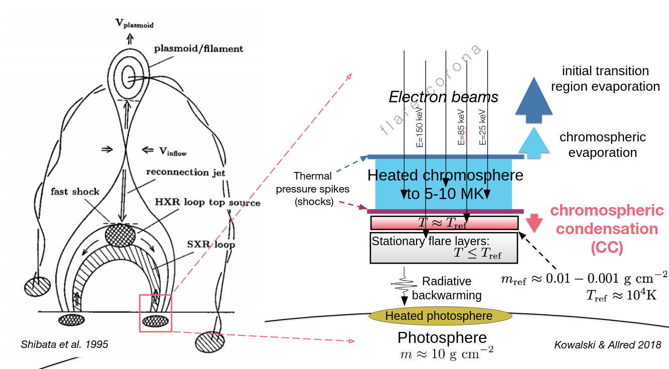
Figure 2: (Left) Illustration of several salient features and processes in the standard model of solar flares, reproduced from Shibata et al [673] with permission. (Right) Generalization of the chromospheric evaporation and condensation phenomena in radiative-hydrodynamic models of high-flux electron-beam heating at the footpoints of newly-reconnected flare loops [adapted from 410]. Here, we also include an illustration of the radiative backwarming of the photosphere, which is predicted by some 1D models [9] of flare chromospheres that are optically thin at Balmer and Paschen continuum wavelengths [see 225, for the expected geometry of 3D radiative backwarming of the photosphere].

In large solar flares, a sizable fraction of the magnetic energy that is released seems to go into accelerating ambient particles (electrons, protons, ions) to mildly relativistic energies [452, 204, 759, 760]. The nonthermal (“beam”) distribution is a power-law extending from $\sim 10$ keV to tens of MeV for electrons and $\sim 1-1000$ MeV for protons. Recent observations have shown that the Sun is a prolific particle accelerator: $\approx 1-100$% of the pre-flare coronal electrons are accelerated [771, 427, 424, 554, 423, 227, 402]. The inferred nonthermal particle flux density into the lower atmosphere can attain a correspondingly extreme range, $\sim 10^{12}-10^{13}$ erg cm^-2 s^-1, at some locations in solar flares [492, 111, 785, 537, 425].

Determining how and where the bulk of nonthermal particles is accelerated in the solar atmosphere is actually a very active research topic [for an overview, see 796]. Generally speaking, there are three classes of particle acceleration that may operate in the solar atmosphere [23, and see also Knuth and Glesener 395 and Chen et al 126 for succinct overviews of the more modern classifications]: first-order Fermi and shock (including shock-drift and diffusive shock), stochastic (“AC”, or resonant interaction with a spectrum of magnetic turbulence), and electric field (“DC”) acceleration. Many theoretical frameworks roughly fall under one of these types in one way or another, and all may operate to some degree over the volume and time-evolution of a flare.

In and around the volume of reconnection and its outflow jets, there have been exciting advances in producing power-laws from multiple first-order Fermi reflections (through curvature-drift motions of particles) among volume-filling plasmoids, which are contracting and coalescing magnetic “islands” [671, 187, 553, 378, 188, 147, 286]. These models have recently been extended to 3D [148] and expanded to much larger physical sizes [189, 21] than particle-in-cell simulations, demonstrating efficient acceleration of high-energy electrons into power-law tails that extend over many orders of magnitude. The Alfvenic-speed reconnection exhaust may develop turbulence, and stochastic acceleration within turbulence [500, 586, 585, 70] in the presence of Coulomb collisions [72] is thought to be one of the possible acceleration mechanisms. Sub-Driecer [e.g., 317, 60, 7] electric fields have also been investigated in accelerating a small fraction of the ambient particles, and super-Driecer electric fields (accelerating the entire ambient population) that result from the observed decay of magnetic field over a large loop-like volume have also been discussed [227], possibly related to a type of hybrid particle acceleration involving electric fields and turbulent reconnection [752]. Despite the apparent lack of consensus among these impressive modeling and theoretical directions, a commonality is that a significant amount of energy is transferred to the atmosphere through shortening of magnetic field lines (facilitated by reconnection), and particles are efficiently accelerated over a large volume. For reviews of magnetic reconnection and particle acceleration, see also [729, 119, 597, 120, 596, 19, 439, 542, 366].

We should mention that acceleration at a coronal termination shock where the reconnection outflow/exhaust collides with the lower-lying (previously reconnected) magnetic loops could also be important [e.g., 690], and plasmoid interaction with a fast-mode MHD shock at the collision interface could contribute to the accelerated particle flux into the lower atmosphere [671]. Acceleration based on terrestrial aurorae or magnetotail sub-storm processes are also considered [75, 290], and some models argue for a mechanism where the bulk of electron acceleration takes place close to [680, 724] or within [230] the chromosphere. Whatever the case or cases may be, acceleration models should attempt to reconcile one way [e.g., 98, and see also Section 3.6 in Aschwanden et al 32] or another [127] with energy-dependent time delays of hard X-rays [31, 33, 32, 22, 602, 13, 395] and the general agreement between inferred path lengths and direct imaging measurements of flare loop sizes. Other critical tests are matching the properties of the white-light continuum radiation [231], reproducing the energy content in accelerated protons [e.g., $E\approx 7\times 10^{32}$ erg above a proton kinetic energy of 30 MeV; 524], and generating strong nonthermal electron radio signatures at coronal heights [126].

In order to consider the rest of the flare process, let us assume that the nonthermal particle beams are injected into a region around the apex of a just-reconnected-and-retracted coronal loop. Initially, the particles are injected in relatively low-lying magnetic fields ($\lesssim 10$ Mm), resulting in the onset of the flare impulsive phase. Over time, larger (and weaker) magnetic fields reconnect and energize particle beams. The particle beams are injected into the newly reconnected loops with a distribution of pitch angles with respect to the magnetic field orientation. The $E\gtrsim 100$ keV electrons in the beams produce gyrosynchrotron radiation as they spiral (with Larmor radii of $\sim$ cm) in the magnetic fields. If the magnetic flux density [G] increases along the beam path (e.g., if the cross-sectional area of the loop correspondingly converges into the lower atmosphere), then the particles with small pitch angles with respect to the magnetic field direction will freely stream (“precipitate”) into the chromosphere. Those with larger initial pitch angles will gradually and adiabatically increase their pitch angle, which is a result of Faraday’s Law of Induction in the frame of the gyrating electrons. These particles can eventually reflect, or “mirror”, at the footpoints (which could occur in the transition region, high chromosphere, low chromosphere, or low corona). After some time, the mirrored particles too will scatter off enough ambient particles in the corona and precipitate out of the magnetic “trap” into the chromosphere. This is the so-called “trap$+$precipitation” paradigm [498]. The highest energy particles take the longest to scatter and thus remain trapped for a time proportional to $\frac{E^{1.5}}{n_{e}}$ where $E$ is the kinetic energy of the nonthermal electrons and $n_{e}$ is the ambient/thermal electron density that the beam heats (under the dilute beam assumption: $n_{\rm{e}}\gg n_{\rm{e-beam}}$). These times are rather short ($<10$ s) for typical conditions and energies. In solar flares, proton/ion beams can certainly contribute to atmospheric heating [598, 11], nuclear excitation, a gamma-ray continuum spectrum, the 2.2 MeV neutron-capture Deuterium-formation line, the 511 keV positron-annihilation line, and neutrons that are directly detected at Earth [524, 751]. For the sake of brevity, we further consider the effects of only accelerated electrons.

When the electron beam particles stream into the chromosphere, they encounter a wall of dense, partially ionized gas to which they rapidly lose their energy through Coulomb collisions with ambient electrons. At the same time, free-free radiative transitions in collisions with ambient protons occur in the chromosphere, producing hard X-ray ($E\gtrsim 25$ keV), nonthermal bremsstrahlung radiation that exhibits a power-law distribution. Hard X-ray light curves define the impulsive phase in solar flares. The standard model of hard X-ray emissivity that accounts for Coulomb energy loss as the electrons radiate bremsstrahlung is called the collisional (cold) thick target model [CTTM; 96, for reviews, see Brown et al 99, Holman et al 320, Kontar et al 400]. Electron beam power-laws that are inferred from the CTTM and injected into radiative-hydrodynamic simulations are typically characterized by power-law indices of $\delta\approx 5$, a low-energy cutoff of $E_{c}\approx 15-25$ keV, and energy flux densities in the range of $\approx 10^{10}$ to $\approx 10^{11}$ erg cm^-2 s^-1 [117]. Often, the hard X-ray light curves consist of gradual variations with superimposed short bursts of $\mathcal{O}(0.5-5)$ s. In some interpretations, these timescales are sensibly related to the processes of prompt and delayed precipitation (described in the previous paragraph) of nonthermal electrons.

The relative displacement of the accelerated electrons from the slower ions in the corona results in a “return current electric field” [e.g., 730, 684]; this electric field drains energy from the beam and transfers it as a drifting velocity component to the ambient Maxwellian distribution of electrons. The drift is towards the loop apex. In steady state, the flux densities ($J$; el s^-1 cm²) of the beam and return current drifting electrons are equal and opposite, thus preventing pulsar-strength, $B\approx 10^{9}$ G, magnetic fields from forming in the solar atmosphere. The resistivity of the background results in “Joule heating” of the coronal plasma [$\approx\eta e^{2}J_{\rm{beam}}^{2}$; 318, 11, 6]. For non-dilute beams, the density of the electron beam is comparable to the ambient electron density, and interactions of plasma wave turbulence and parallel electric fields (e.g., Langmuir waves, electrostatic double layers) with the beam are additionally expected.

The nonthermal electron beam kinetic energy is thermalized in the low corona and mid-to-upper chromosphere; see right side of Figure 2. Initially hydrogen primarily provides the radiative cooling that balances the chromospheric temperature increase. As the chromosphere increases from $T\approx 8000$ K to $T\approx 30,000$ K, hydrogen becomes fully ionized, and then helium I and helium II take over the radiative cooling in the range of $T\approx 30,000-80,000$ K. Thus, it is thought that non-equilibrium rates of helium and detailed radiative transfer are important for calculating accurate evolutionary states of the atmosphere. After helium is fully ionized, oxygen, carbon, and neon regulate the cooling at $T\approx 10^{5}$ K, which is the peak of the optically thin cooling curve [e.g., 139, 639, 168, 174]. If enough heat is deposited to fully ionize these elements, then a temperature runaway, or explosion, ensues because the optically thin cooling decreases as a function of temperature up to $T\approx 20$ MK. Thermal conduction transports energy away from the region of maximum beam deposition. Thus, the temperature “bubble” expands, resembling a one-dimensional blast wave (which is more or less confined to the magnetic field direction) in an exponential atmosphere with pervasive beam heating. The increased pressures and their gradients result in a multitude of mass motions. Additionally, an increase in temperature of the very low corona (through thermal heat conduction) can also drive mass motions on top of the beam-generated mass motions. The sources and sinks of the equation for energy conservation are discussed further in Sect. 9.

The impulsively-generated upflows and downflows have been studied numerically as part of the standard solar flare paradigm for many decades [458, 224, 223, 222, 220]. They are respectively known as explosive chromospheric evaporation and chromospheric condensation (Figure 2, right). The condensations and evaporations manifest as redshifts and blueshifts in cool and hot lines, respectively, with a transition temperature that has been constrained in solar flares [501]. The high-speed upflows fill the loops with $T\approx 10-30$ MK plasma, while the higher density downflows accrue/accrete mass over time and radiatively cool through $T\approx 10,000$ K (i.e., this is a non-adiabatic process). The chromosphere is compressed as in a snow plow effect while also experiencing continuous energy deposition directly by the beam. The condensations are a result of shock phenomena because they increase in density up to 10x the ambient density (whereas sound waves would ostensibly smooth out the density perturbations). The closest physical process to the temperature bubble and condensation that we have found [e.g., 421] is that of a thermal wave [Section 6.6, pp 671-672 of 793, and see also Atzeni and Meyer-ter Vehn 37 for similarities to supersonic ablative heating waves in laboratory implosion experiments], which are described as a “second-kind temperature wave” in Livshits et al [458].

The representative properties of the condensation and evaporation flows at any time in the evolution follow from a simple momentum balance equation:

$$\left(v\rho\Delta z\right)_{\rm{cond}}\approx-\left(v\rho\Delta z\right)_{\rm{evap}},$$ (2)

where $\Delta z$ is a physical depth range over which gas with a mass density of $\rho$ has a bulk velocity of $v$.

Here, we ignore the downward momentum of proton and electron beam particles [349, 10]. Typical values of the condensation are $\Delta z\approx 30$ km [which scales inversely with surface gravity; 410] and $v\approx-50$ km s^-1. Typical evaporation flows are fully ionized and have $n_{e}\approx 10^{11}$ cm^-3 ($\rho\approx 3\times 10^{-13}$ g cm^-3) with flow speeds of $v\approx 100-500$ km s^-1. The density of the condensation increases over time, which is compensated by an increase in the $\Delta z$ of the evaporation as chromospheric/transition region mass ablates into and fills the newly-reconnected magnetic loop. After the flows fill up a $\Delta z\approx 10$ Mm loop, then Equation 2 implies a gas density of $10^{-9}$ g cm^-3 in the condensation, in agreement with numerical simulations. The coronal loops thus emit in soft X-rays, while the footpoints emit in optical and UV radiation. The condensation manifests as red-shifts in broad, chromospheric lines (Fe II, Mg II, H$\alpha$, Si II) that exhibit a red-wing asymmetry (RWA). The RWA evolves in velocity and intensity over $\approx 30$ s [349, 792, 785, 274].

[220] calculated the analytic relationship between the beam energy flux deposited above the flare transition region ($F_{\rm{evap}}$), the peak downflow (condensation) speed ($v_{\rm{peak}}$) just below the flare transition region, and the pre-flare chromospheric mass density ($\rho_{\rm{chrom}}$) at which the flare transition region forms:

$$v_{\rm{peak}}\approx 0.6\big{(}\frac{F_{\rm{evap}}}{\rho_{\rm{chrom}}}\big{)}^{1/3}$$ (3)

Typical upflows of $100-500$ km s^-1 imply durations up to $\approx 30-90$s to fill a flare loop, at which time the confined, field-aligned flows from conjugate footpoints collide. Superhot (lower volume and lower density) $T\approx 30-50$ MK sources can be produced above the looptops of the cooler, $T\approx 20$ MK, plasma that is thought to be due to chromospheric evaporation; these are thought to be due to heating from slow-mode (Petschek) shocks in reconnection, as demonstrated in recent multi-dimensional MHD simulations [e.g., 461]. However, some of such sources that are consistent with ultrahot $100-200$ MK thermal spectra that appear early on are generally more consistent with nonthermal power-law spectra.

In the impulsive phase, bright sources are observed from the footpoints (Figure 2, right) of flare loops in cooler emission lines and in the UV, optical, and infrared continuum radiation. A variety of source morphologies appear and could be affected by temporal and spatial resolution. However, one can typically separate the geometry into elongated “ribbons” and compact, brighter circular “kernels” [see, for example, the remarkable H$\alpha$ images in 384]. Within a relatively short time, the footpoints light up quasi-sequentially along the PIL, forming flare ribbons [e.g., 603, 386]. One ribbon typically develops in plage, and another ribbon develops in a penumbral or umbral region of sunspot. As the flare progresses, the distance between the two ribbons increases, which is the so-called perpendicular apparent motion. This is thought to be a signature of the reconnection occurring higher and higher in the corona, thus releasing energy from larger and larger loops, which is a hallmark of the famous “CSHKP” model of two-ribbon flares [118, 701, 316, 403]. As a result, the brightest emission is generally seen at the “leading bright edge” of the ribbons as they spread apart (Figure 2 left). It is thought that excitation from above, e.g. through particle beams, changes location rather than through cross-field thermal heat transport / diffusion in the low atmosphere. However, radiative backwarming from the X-ray, EUV, and FUV lines may play an important role in heating the surrounding atmosphere away from the brightest kernels [such as in the so-called “core-halo” morphology; 537, 9, 357, 225, 528]. After the excitation front passes, the impulsively-generated chromospheric condensation continues to propagate even in the absence of electron beam heating, but it eventually reaches pressure equilibrium with the lower atmosphere. The loops cool from tens of MK to 1 MK, first primarily through thermal conduction, then primarily through radiation, resulting in the appearance of the famous “post-flare” loops as seen in filtergrams such as AIA 171 Å  (which are, really, post-impulsive phase loops; see Fig. 3 and Liu et al 456). In cooler lines such as H$\alpha$ or He II 304, the very late phase of each flare loop is sometimes associated with the phenomena of coronal rain, which is a second phase of “condensation”. In this phase, dense material that was chromospheric before the flare drains out of the corona. New flare loops are continuously formed through the gradual decay phase of GOES soft X-ray solar flares [762], but the details of the partition among various possible heating sources in the low atmosphere (thermal heat flux, electron beams, proton beams, direct heating by waves) remain poorly understood, especially during stellar flares. We note that the origin of the long cooling times of post-flare loops on the Sun is still a very active area of research [e.g., 645, 457, 600, 71, 798, 389, 612, 12, 35].

Several notable and well-studied solar flares are the SOL1992-Jan-13T17:25 M2.0 flare [“the Masuda flare”; 481], the SOL2000-Jul-14T10:00 X5.7 flare [“the Bastille Day flare”, e.g., 601], the SOL2003-Oct-28T11:30 X17 flare [one among the “the Halloween storms”, e.g., 778], the SOL2002-Jul-23T00:30 X4.8 [ “double power-law”; 319] flare, the SOL2014-Mar-29T17:48 X1.0 flare [NASA’s “best observed X-class flare”; e.g., 392], the SOL2014-Sep-10T17:45 X1.6 flare [e.g., 273], and the SOL2017-Sep-10T16:06 X8.2 flare [e.g., 126].

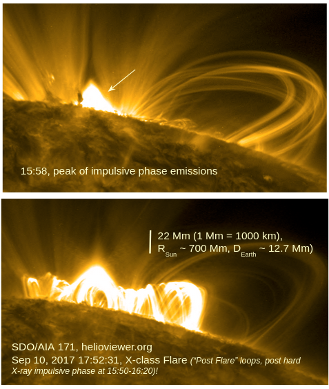
Figure 3: SDO/AIA images around the EUV wavelength of $171$ Å [442], obtained from Helioviewer.org, showing thermal emission from flare loops at two times during a large X-class flare on the solar limb. The top panel shows the compact, low-lying thermal flare arcade (indicated by the arrow) during what is usually the peak of the nonthermal hard X-ray (not shown) luminosity from the footpoints. Later in the flare, the bright arcade volume exhibits an expansion horizontally and vertically – the expansion is, however, apparent in the sense that newly reconnected, larger magnetic loops participate in the flare as time progresses. The large arcades have traditionally been called “post-flare” loops, which shine brightly much longer after the end of the main hard X-ray impulsive phase (they are perhaps more accurately called “post-nonthermal-X-ray-footpoint” loops). It is generally thought that the flare loops in these images are the result of magnetic structures that have cooled down from much higher temperatures to $T\approx 1$ MK [e.g. 28]. Note that a cusp-like (fork-shaped) dark region just above the bright loops in the top panel is where many models and observations suggest that the bulk of magnetic reconnection and particle acceleration occur [see 462, 126]. For illustrative comparisons of flare and active region loops, see [276].

4 A Survey of Flare Stars

The characteristics that lead to flaring in stellar atmospheres are generally thought to be some combination of the following: rapid rotation, an outer convective zone, and disorganized surface magnetic fields. The ratio of stellar rotation to the convective turnover time is called the Rossby number, or the inverse Coriolis number, which may be indicative of how much internal shear, differential rotation, and turbulent amplification of kinetic energy into magnetic energy contribute to the dynamo. The dynamo may operate in the shear flows around the tachocline interface, and/or throughout the turbulent convection zone, and/or in the near-surface shear layers. Stars with small Rossby numbers are found in the so-called “saturated regime” of quiescent magnetic activity (outside of large flares). The saturated regime is empirically characterized by nearly constant luminosity ratios of $L_{X}/L_{\rm{bol}}\approx 10^{-3}$ (Figure 4) and $L_{H\alpha}/L_{bol}\approx 10^{-4}$ [e.g., 594, 781, 621, 770, 780, 541, 102, 782], where $L_{\rm{bol}}$ is the quiescent bolometric luminosity, and the numerator is a luminosity [e.g., the soft X-ray luminosity, $L_{X}$; 659, 781] that is a proxy for magnetic heating in the corona or chromosphere. There is a rather large spread about the saturated value from star to star, and the Sun varies from $L_{X}/L_{\rm{bol}}\approx 5\times 10^{-8}$ to $\approx 5\times 10^{-7}$ over its 11 year sunspot cycle [369, 42]. For comparison, the least active M dwarfs have ratios of $10^{-6}$ [780, 235, 94, 205]. At very small Rossby numbers, a super-saturated regime may occur, while stellar activity proxies follow a power-law with increasing Rossby numbers $\gtrsim 0.1$, relatively independent of spectral type For an introduction to dynamo theory in the stars and the Sun, see [84], [85], [125], [102], and [664]. For a review of the literature, see [102] and [373]. Much recent progress has been made in modeling stellar dynamos in low-mass stars just below [73, 74] and above [101, 95, 372] the fully convective transition, and with especially high-resolution simulations of the solar magnetic field and differential rotation [325].

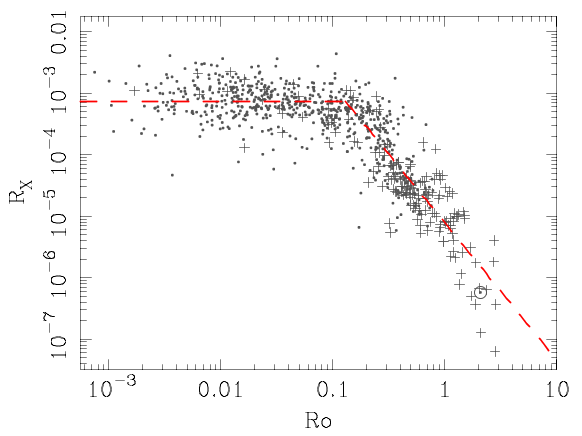
Figure 4: Quiescent $R_{X}=L_{X}/L_{\rm{bol}}$ vs. the Rossby number for a large sample of stars, reproduced from Wright et al [781] with permission. $R_{X}$ is “saturated” at $\approx 10^{-3}$ for stars with Rossby numbers $\lesssim 0.1$, and $R_{X}$ decreases according to a power-law for lower-activity stars.

Magnetic fields buoyantly rise through the stellar photosphere; once in the corona, they undergo destabilization and reconnection to release energy into the atmosphere to produce flares. Flaring occurs at different times through stellar evolution as convective envelopes come and go with changes in internal structure, core fusion processes, and external factors such as tidal locking and synchronous rotation. An overview of the myriad of flare stars is best summarized in a color-magnitude diagram (CMD). Prolific and/or representative flare stars are shown on a Gaia CMD in Fig. 5. The data were obtained from Gaia Data Release 2 [246], except for a few cases that are only available through the Early Data Release 3 or through common filter transformations [737] for some of the brightest stars. The background data are the Gaia photometry for a collection of stars compiled for the Palomar/Michigan State University spectroscopic survey [PMSU; 618, 299, 264, 619, 617], downloaded from Neill Reid’s website. Many of these stars are discussed in the recent 10 pc Gaia sample [624] and the CNS5 catalog [268]. Isochrones from the PARSEC v1.2S [89] stellar evolution models are shown for solar age and metallicity and the age of the $\beta$ Pic moving group [478]. Characteristics of selected flare stars in the CMD are summarized in Tables 1 - 6, and in some cases a reference to an example of a flare study featuring the respective star.

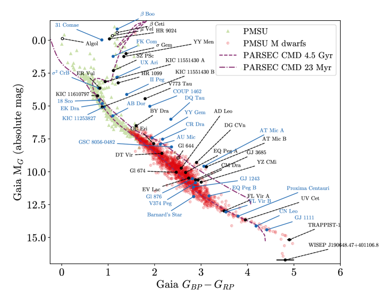
Figure 5: Gaia color-magnitude diagram of absolute magnitude vs. color for notable flare stars (outside of flaring). Note that corrections for extinction and reddening from interstellar dust are not applied because most of these stars are in close proximity (within $\sim 20$ pc) of Earth. The linecolors and linestyles for the annotations are arbitrary. Open circles signify that the data were transformed from Hipparcos magnitudes and/or parallaxes. Several solar-metallicity isochrones from the PARSEC stellar evolutionary models are shown for reference.

Table 1: Table of common and notable flare stars.

Name	SpT	Class	$d$	Gaia $G$	$U$	RA, Dec	Ref
			(pc)	(app mag)	(app mag)	(J2000)
dMe / UV Cet
YY Gem (Gl 278C)	M0+M0	BY Dra/EB	15.0984	8.3	11.6	07 34 37, +31 52 10	[180],[696]
DT Vir (Gl 494)	M1	dMe	11.5132	8.91	12.3	13 00 46, +12 22 32
AU Mic (Gl 803)a	M0/M1	(d)Me	9.7248	7.84	11.3	20 45 09, -31 20 27	[145], [722]
CR Dra (GJ 9552)b	M1	dMe	20.2626	9.06	12.0	16 17 05, +55 16 08	[767]
SDSS J211827.00	M1	dMe/S82	711.9443	17.01	…	21 18 27, +00 02 48	[411]
+000248.5c
SDSS J005903.60-	M1	dMe/S82	123.2745	13.89	…	00 59 03, -01 13 31	[411]
011331.1
Gl 411	M2	dMe	2.55	…	10.1	11 03 20, +35 58 11	[39]
VV Lyn (Gl 277A)	M2.5	dMe	11.86	…	…	07 31 57, +36 13 09
AD Leo (Gl 388)	M3	dMe	4.966	8.21	11.9	10 19 36, +19 52 12	[297]
GQ And (Gl 15B)	M3.5	dMe	3.5614	9.68	…	00 18 25, +44 01 38
EQ Peg A (Gl 896A)	M3.5	dMe	6.2614	9.04	13.2	23 31 52, +19 56 14	[447], [416]
EV Lac (Gl 873)	M3.5	dMe	5.0502	9.00	13.0	22 46 49, +44 20 02	[567]
GJ 3685	M4	dMe	18.7988	11.98	…	11 47 40, +00 15 20	[632]
GJ 1243	M4	dMe	11.9787	11.55	15.5	19 51 09, +46 29 00	[304]
DG CVn (GJ 3789)	M4+M4	(d)Me	18.2857	10.61	…	13 31 46, +29 16 36	[571]
BL Lyn (Gl 277B)	M4	dMe	12.001	10.47	…	07 31 57, +36 13 47
V374 Peg (GJ 4247)	M4	dMe	9.1041	10.63	…	22 01 13, +28 18 24	[741]
YZ CMi (Gl 285)	M4.5	dMe	5.9874	9.68	13.8	07 44 40, +03 33 08	[412]
EQ Peg B (Gl 896B)	M4.5	dMe	6.2477	10.82	$\approx$15	23 31 52, +19 56 14	[635], [487]
AT Mic A	M4.5	(d)Me	9.8816	9.56	…	20 41 51, -32 26 06	[251]
AT Mic B	M4.5	(d)Me	9.8312	9.59	…	20 41 51, -32 26 10	[251]

Table 2: Continued …

Name	SpT	Class	$d$	Gaia $G$	$U$	RA, Dec	Ref
			(pc)	(app mag)	(app mag)	(J2000)
V639 Her (Gl 669B)	M4.5	dMe	10.7566	11.46	…	17 19 52, +26 30 02
AF PSc (GJ 1285)	M4.5	dMe	34.957	12.81	…	23 31 44, -02 44 39	[767]
CM Dra (Gl 630.1)	M4.5+M4.5	dMe/EB	14.85	11.5	…	16 34 20, +57 09 44	[511, 432]
GJ 1245A	M5	dMe	4.6919	11.47	…	19 53 54, +44 24 51	[466]
GJ 1245B	M5	dMe	4.6614	11.92	…	19 53 55, +44 24 54	[466]
FL Vir (Wolf 424 AB/Gl 473AB)	M5+M7	dMe	4.40	11.24	15.4	12 33 17, +09 01 15
CU Cncd (GJ 2069)	M3.5+M3.5	dMe/EB	16.6012	10.55	…	08 31 37, +19 23 39
SDSS J025951.71	M5	dMe/S82	106.8607	15.87	…	02 59 51, +00 46 19	[411]
+004619.1e
Prox Cen (Gl 551)	M5.5	dMe	1.3012	8.95	14.3	14 29 42, -62 40 46	[283]
CX Cnc (GJ 1111)	M6	dMe	3.5805	12.19	19.0	08 29 49, +26 46 33	[313]
UV Cetif (Gl 65B)	M6	dMe	2.687	10.81	…	01 39 01, -17 57 01	[197]
CN Leo (Gl 406)	M5.5-6	dMe	2.4086	11.04	17.03	10 56 28, +07 00 52	[661]
SDSS J001309.33	M6	dMe/S82	48.2787	15.93	…	00 13 09, -00 25 51	[411]
$-$002552.0g

Table 3: Continued …

Name	SpT	Class	$d$	Gaia $G$	$U$	RA, Dec	Ref
			(pc)	(app mag)	(app mag)	(J2000)
Ultracool dMe / VLMh
VB8 (Gl 644C)	M7	dMe	6.5014	13.84	…	16 55 35, -08 23 40
VB10 (Gl 752B)	M8	dMe	5.9185	14.32	…	19 16 57, +05 09 01	[371]
TRAPPIST-1	M8	dMe	12.4299	15.65	…	23 06 29, -05 02 29	[742]
Gaia DR2 87125610-	M8	…	75.5971	19.28	…	02 21 16, +19 40 20	[655]
622839424
WISEP J190648.47	L1	…	16.7867	17.84	…	19 06 48, +40 11 08	[265]
+401106.8
Optically inactivei dM
Gl 832j	M1.5	dM	4.9651	7.74	11.5	21 33 33, -49 00 32
Gl 674	M2.5	dM	4.5496	8.33	12.0	17 28 39, -46 53 42	[237]
Barnard’s star (Gl 699)	M4	dM	1.8266	8.2	12.5	17 57 48, +04 41 36	[235],[579]
IL Aqr (Gl 876)	M4/5	dM	4.6758	8.88	12.9	22 53 16, -14 15 49	[234]
YSO’s and Pre-Main Sequence
GSC 8056-0482k	M2	…	38.8466	11.06	…	02 36 51, -52 03 03	[465]
V773 Tau	…	T Tau	128.1264	9.98	…	04 14 12, +28 12 12	[480]
DQ Taul	…	T Tau	197.4475	12.49	$\approx 15.5$	04 46 53, +17 00 00	[258, 715]
COUP 1462	…	YSO	376.405	12.9	…	05 35 31, -05 15 33	[257]

Table 4: Continued …

Name	SpT	Class	$d$	Gaia $G$	$U$	RA, Dec	Ref
			(pc)	(app mag)	(app mag)	(J2000)
Active Binary
HR 1099 (V711 Tau)	G5IV/K1IV	RS CVn	29.6272	5.6	…	03 36 47, +00 35 15	[566]
II Peg	K2-3V-IV/??	RS CVn	39.363	7.1	…	23 55 04, +28 38 01	[568]
$\sigma$ Gem	K1III/??	RS CVn	37.0194	3.86	…	07 43 18, +28 53 00	[100]
ER Vul	G0V+G5V	RS CVn	50.7822	7.18	…	21 02 25, +27 48 26
$\sigma^{2}$ CrB	F6V+G0V	RS CVn	22.658	5.41	…	16 14 40, +33 51 31	[565]
V824 Ara	G5IV+K0V-IV	RS CVn	30.5063	6.45	…	17 17 25, -66 57 03
V815 Her	G5V+M1-2V	RS CVn	32.396	7.32	…	18 08 16, +29 41 28
EI Eri	G5IV/??	RS CVn	55.068	6.95	…	04 09 40, -07 53 34
AR Lac	G2IV	RS CVn	42.6744	5.89	…	22 08 40, +45 44 32
BH CVn	F2IV/K2IV	RS CVn	46.1482	4.73	…	13 34 47, +37 10 56
CF Tuc	G0V/K4IV	RS CVn	87.9555	7.45	…	00 53 07, -74 39 05
UX Ari	K3-4V-IV/??	RS CVn	50.4723	6.33	…	03 26 35, +28 42 54	[282]
VY Ari	K3-4-IV/??	RS CVn	41.2999	6.61	…	02 48 43, +31 06 54
AR Psc	K2V/??	RS CVn	45.9586	7.03	…	01 22 56, +07 25 09
Lambda And	G8IV-III/??	RS CVn	24.1695	3.26	…	23 37 33, +46 27 29
SZ PSc	K1IV+F8V	RS CVn/EB	90.1098	7.08	…	23 13 23, +02 40 31	[376]
CC Eri	K7V+M4V	RS CVn/BY Dra	11.5373	8.17	…	02 34 22, -43 47 46	[374]
ER Vul	G0V+G5V	RS CVn	50.7822	7.18	…	21 02 25, +27 48 26
EI Eri	G5IV+dM	RS CVn	55.068	6.95	…	04 09 40, -07 53 34
KIC 11551430 Am	…	…	324.4975	10.7	…	19 09 40, +49 30 05	[473]
KIC 11551430 B	…	…	321.2161	12.62	…	19 09 40, +49 30 05	[473]

Table 5: Continued …

Name	SpT	Class	$d$	Gaia $G$	$U$	RA, Dec	Ref
			(pc)	(app mag)	(app mag)	(J2000)
Single Evolved / Active Giants
HR 9024	G1III	Gap	139.485	5.62	…	23 49 40, +36 25 31	[710]
FK Com	G5III	Gap	216.9119	7.91	…	13 30 46, +24 13 57
v Peg	F8III	Gap	2705.5292	9.84	…	22 01 02, +06 07 11
31 Comae	G0III	Gap	87.0072	4.67	…	12 51 41, +27 32 26
EK Eri	G8IV	Gap	64.1692	6.07	…	04 20 38, -06 14 45
$\beta$ Ceti	K0III	Clump	29.53	$\approx 1.77$	3.90	00 43 35, -17 59 11	[47]
Gamma Tau	G9.5III	Clump	44.202	3.29	…	04 19 47, +15 37 39
$\theta^{1}$ Tau	G9III	Clump	46.689	3.49	…	04 28 34, +15 57 43
$\beta$ Boo/ Nekkar	G8 III	Pre-RG?n	62.7702	3.14	5.2	15 01 56, +40 23 26	[347]
YY Men	rapid	FK Com	216.6981	7.92	…	04 58 17, -75 16 37
$\mu$ Vel	G6III(+ dF)	Pre-RG	35.7812	$\approx 2.35$	4.16	10 46 46, -49 25 12	[46]
Dwarf K starso
AB Dor	K0V	Ke	15.3093	6.67	…	05 28 44, -65 26 55	[476]
BY Dra	Ke+Ke	BY Dra	16.5108	7.59	…	18 33 55, +51 43 08
$\epsilon$ Eri	K2V	…	3.2029	3.37	…	03 32 55, -09 27 29

Table 6: Continued …

Name	SpT	Class	$d$	Gaia $G$	$U$	RA, Dec	Ref
			(pc)	(app mag)	(app mag)	(J2000)
Young Solarp
EK Dra	G1.5V	solar	34.4502	7.5	…	14 39 00, +64 17 29	[43]
KIC 11610797	G	solar	279.3635	11.46	…	19 27 36, +49 40 14	[473]
KIC 11253827	G	solar	225.1926	11.83	…	19 44 31, +48 58 38	[473]
KIC 10422252	G	solar					[675]
KIC 12023498	…	…	530.1268	12.12	…	19 47 02, +50 27 18	[87]
KIC 8164653	…	…	3816.1876	14.32	…	19 25 36, +44 05 10	[87]
KIC 8803106	…	…	867.4893	13.79	…	18 57 37, +45 05 13	[87]

Stellar classification according to binarity, evolutionary status, and spectral type is important for understanding the origin and release of magnetic energy. We describe general classifications of the types of stars that flare across the CMD (Fig. 5). In the following “early” spectral types refer to those of hotter effective temperatures (e.g., M0-M2), and “later” spectral types refer to the cooler effective temperatures (e.g., M7-M9); this jargon has no direct correspondence to time or age. Mid-type M dwarfs span the fully convective transition and roughly correspond to stars with spectral types $\approx$ M3-M6, though there is over an order of magnitude range of bolometric luminosities just within this sub-grouping.

• RS CVn. Though rapid rotation is often associated with stellar youth, tidal locking of binaries can lead to prolonged magnetic activity and enhanced flare rates for billions of years [570] in systems that would not normally produce energetic events. RS CVn systems are synchronously rotating, detached binaries consisting of an early-type main sequence star and an evolved, cooler G/K sub-giant or giant companion. In RS CVn systems, the flares are thought to originate from the cooler component. The cool star component has a large convection zone, which combined with very rapid rotation for its size, leads to large flares with rise and decay times on the order of days. The flares of RS CVns are among the highest energy ($10^{36}-10^{37}$ erg) and longest-lasting stellar flares. Flare rates from the EUV and X-rays indicate about one flare per day [561], but optical enhancements are relatively rare due to the enormous background glare from the non-flaring source; peak $U$-band changes (Equation 1) are typically much less than a magnitude for energies of $E_{U}>10^{33}$ erg [rates of $\approx 0.17$ hour^-1; 484]; the largest flares increase the $U$-band flux by a factor of $\approx 2$ [181]. The best-studied RS CVn system is arguably HR 1099 (V711 Tau), which consists of a primary K1 IV (sub-giant) and a G5 V (main sequence) star with orbital separation of $\approx 3R_{\rm{Sun}}$ and a 2.8 day synchronized orbital and rotation period [217]. The most extensive multi-wavelength study of the flaring and quiescence of RS CVns is presented in [561, 563, 564, 565, 566]. A large catalog of the non-flaring properties of these stars is contained in [700].

• Algol-type flare stars are semi-detached binaries with a history of significant mass transfer from a cool evolved sub-giant onto a main sequence B-type star. Algol (B8V + G8III/K1IV/K2III) consists of eclipsing binary (EB) stars separated by 14.14$R_{\rm{Sun}}$, whose components have radii of 2.9 and 3.5$R_{\rm{Sun}}$ with a 2.87-day orbital period. Algol produces giant flares on occasion [732, 212], and serendipitous eclipses of the flares constrain the geometries and locations of the events on the cooler, less-massive subgiant component, Algol B [658, 660], which is also the source of the coronal radio emission [445]. Algol B is one of the few stars besides the Sun whose magnetosphere has been spatially resolved in radio observations [583]. Detailed comparisons of Algol-type and RS CVn systems have been presented in [682, 650, 190]. They are otherwise quite similar, except the total optical (non-flaring) light from the system is dominated by the main sequence B star in Algol-like systems, whereas RS CVns consist of two cool stars (spectral type G or later) with one subgiant or giant star that dominates the total system light. The different locations on the CMD (Fig. 5) are clear.

• BY Dra-type stars are, here, informally referred to as closely orbiting (EB or non-EB), detached binaries consisting of two main-sequence, typically late K or early M, stars. Arguably, the best known BY Dra flare star is the eclipsing 0.8 day period binary YY Gem, which consists of nearly identical, and probably rotationally synchronized, dM0e stars with radii of $\approx 0.6R_{\rm{Sun}}$ and masses of $\approx 0.6M_{\rm{Sun}}$ separated by 3.83 $R_{\rm{Sun}}$ [720, 214, 105, 397]. Other eclipsing BY Dra flare star systems are CM Dra and CU Cnc. BY Dra itself is composed of two active main-sequence K stars with semi-major axes of $7.4-8.4\times R_{\rm{Sun}}$ and pseudo-synchronous rotation with a period of 5.9 d [310]. Formally, BY Dra is a term that describes the class of magnetically active spotted stars that exhibit periodic variation in their optical light curves, due to starspots and rotational modulation [General Catalogue of Variable Stars: Version GCVS 5.1; 649]); however, the BY Dra classification more uniquely describes [e.g., 617] detached active binary systems that consist of main sequence late-type (K or M) stars that orbit very closely together, like BY Dra itself.

• Pre-Main Sequence (PMS) stars, such as Young stellar objects (YSO’s) and T Tauri stars exhibit flaring emission [e.g., 226] in addition to the emission from accretion: the flow, shocks, and hotspots at the stellar surface all generate optical, UV, IR, and X-ray continuum and emission line radiation [e.g. 312] that can be both steady-state and transient. The optical, NUV, and FUV flares on T Tauri stars tend to be very energetic, $\gtrsim 10^{35}$ erg [715, 315, 259]. [715] conducted a large optical photometric monitoring campaign on the T Tauri binary star DQ Tau and compared the color differences between accretion and flare variations. [258] performed an extensive study of X-ray giant flares in the DQ Tau system. The Chandra Orion Ultradeep Project [COUP; 256] detected many X-ray superflares from YSOs; the flares produced X-ray hardness ratios consistent with coronal temperatures of $T>10^{8}$ K [257]. M-type stars take longer to contract onto the main sequence after losing their gaseous disks and are thus not actively accreting, but may exhibit inflated radii for tens of Myr (e.g., AU Mic) as they are still contracting. These are still PMS stars but are also often considered as dwarf, UV Ceti-type stars.

• UV Ceti-type stars are low-mass, M-type main sequence (dwarf) flare stars that exhibit frequent flaring and H$\alpha$ in emission in quiescence [255]. There is a high correspondence between the dMe status and high flare rates [411]. These stars are traditionally denoted as “dMe” or “MVe” stars, they exhibit optical rotational modulation (with periods typically in the $0.2-5$ day range, but see West et al 770 and Newton et al 541), and many but not all are in the saturated regime ($L_{x}/L_{\rm{bol}}\approx 10^{-3}$) of quiescent X-ray luminosity. Many of the UV Cet/dMe-type stars are in the early stages of their main sequence evolution and are possibly only several hundred Myr or less in age. UV Ceti itself is a triple star system with two dM5.5e stars (A and B components) separated by 5.3 au [63]; UV Ceti B is a binary BY Dra-type system (using our adopted definition above). This category includes some non-accreting PMS stars (AU Mic, AT Mic). A catalog of UV Ceti stars and their quiescent properties was compiled by [255] and is provided on VizieR. Though the M-dwarfs are the most populous stars in the Galaxy [e.g., 617], none are visible to the naked eye ($V\lesssim 6$) from Earth due to their low quiescent luminosities.

• Very Low-Mass (VLM) Stars, Ultracool dwarfs, Brown dwarfs. The spectral types M7 through early L span the edge of the core-hydrogen burning regime (i.e., the star/brown-dwarf boundary). The exoplanet host star TRAPPIST-1 is now a well-known, M8 flare star, due to its system of planets in or around the traditional habitable zone [263, 5]. VB 10 is another prolific VLM flare star [311, 454, 229, 371]. The G’́udel-Benz relationship [278] is a correlation between the quiescent radio and soft X-ray fluxes that holds over many orders of magnitudes but breaks down in the VLM regime (with the VLMs being radio overluminous compared to the X-rays). Nonetheless, flares from VLMs and L-type stars have shown dramatic optical continuum enhancements and broad and bright H$\alpha$ lines [446, 653, 265] that otherwise resemble the very energetic flares from the earlier M dwarf spectral types, as noted by [617]. White-light flare rates and magnitude variations have been rather well-characterized recently in time-domain surveys [e.g., ASAS-SN, Kepler, K2, NGTS; 655, 656, 266, 742, 575, 576, 359, 577]. The L-dwarf flare luminosities are remarkably super-bolometric and exceed magnitude changes of $-9$ in the $V$-band [655]. X-ray superflares have been reported from L dwarfs [e.g., 163] as well.

• Weakly active and “inactive” M dwarfs (dM or MV) stars are “optically inactive” stars without H$\alpha$ in emission during quiescence. The inactive dM’s also flare on occasion [579, 411]. These are thought to be descendants of MVe stars, which are inferred to hold on to their high levels of activity for several billion years [301, 769, 391]. After several Gyr on the main sequence, the M-dwarf stars maintain a lower level of chromospheric emission in Ca II H & K (with sometimes H$\alpha$ showing a deeper absorption profile), Mg II h & k emission lines, transition region emission (e.g., C II), and faint X-rays. One notable example of a low-activity M dwarf is the $\approx 10$ Gyr-old, slowly rotating ($P\approx 150$ d) star Gl 699 [Barnard’s star; 755, 233, 716, 235]. Optical flares are rare [313, 304] on optically inactive stars, which do not exhibit much if any rotational modulation in Kepler. The visibility (contrast) of flares at shorter wavelengths is much greater, however, and thus the FUV and X-ray flares are rather prolific [463, 234, 464, 237, 235, 94].

• Solar-type stars Flares from solar-type, G-dwarf stars have been observed rather infrequently, and mostly through serendipitous means in the FUV [44], X-ray [257, 599], and optical [651, 472]. The detectable flares above the spatially integrated, background luminosity are very energetic, and in almost all cases they exceed broadband optical energies of $E>10^{33}$ erg. Detailed flare rates in the EUV have been studied for the rapidly rotating, young, single G-type stars, EK Dra, 47 Cas, and $\kappa$ Ceti [39].

  The Kepler and K2 missions have transformed our knowledge about the white-light flare rates of G-type stars. The literature has been summarized in detail by [136] and [307], and we refer the reader to these works. Here, we provide only a brief synopsis. After the discovery of G-dwarf white-light superflares in Kepler [472], [675] and [548] performed a comprehensive flare rate analysis of the 30-minute cadence data (with some comparisons to the 1-minute cadence data), and [109] extended analyses to lower mass K and M stars [see also 756, for analyses of 30-minute cadence data of M star flares]. [789] also compares short and long cadence Kepler data. [547], [544], and [377] began the detailed spectroscopic characterization of the chromospheric and photospheric properties of the solar-type superflare stars reported in [472] and [675]. [549] and [550] presented spectroscopic follow-up of 46 of the flare stars with 30-minute cadence data in Shibayama et al [675]. [473] analyzed 1-minute cadence data of 23 solar-type superflare stars. The most prolific flare star (KIC 11551430; Table 4) was confirmed as a visual and spectroscopic binary in [551], who presented spectroscopic follow-up of 18 of these 23 stars, leveraging Gaia DR2 data as well to constrain evolutionary statuses on the subgiant branch or main sequence. [555] re-analyzed all solar-type Kepler data and presented up-to-date flare rates. As a result of the group’s detailed follow-up, the calculated superflare occurrence rates on Sun-like stars ($T_{\rm{eff}}=5600-6000$ K, $P_{\rm{rot}}=20-40$ d) has decreased by $\approx$ an order of magnitude since [675]. These refined constraints provide interesting comparisons to extrapolated, multi-wavelength scaling relations from smaller solar flare energies and from large solar energetic particle events [see also, e.g., Figure 33 of 728]. [783] presented flare rates and power-law indices for 77 individual G stars that produce superflares, including KIC 10422252 which is the prolific flare star that is discussed in [675]. [155], [734], and [788] present Kepler flare catalogs, where the latter includes all spectral types including A-type stars (see below) and only long-cadence data. [438] discussed source contamination in the [155] catalog in the higher mass stellar range. Recently, [30] analyzed the power-law distributions of the Kepler long-cadence data flare catalog of [788] and tested against self-organized criticality theory [26].

• Single Active Giants [681] are classified into one of two general categories [see 45]. The first type is helium core burning (post Helium flash) red clump active giants like $\beta$ Ceti. Giant flare events with rise times of $\sim 1$ day are observed from these stars: an impressive EUV light curve of $\beta$ Ceti is shown in Fig. 6 from [47]. The active clump stars are rotating slower than evolutionary models predict, yet they have detectable magnetic fields (unlike the rest of this stellar population). The origin of the magnetic activity in these stars is not well understood, but it has been hypothesized that swallowing a companion planet or brown dwarf increases the shear in the stellar interior [678], resulting in “magnetic rejuvenation” in old age. An alternative idea is that these stars, like some other active giant stars [698], are descendants of Ap stars with strong fossil fields [725]. The second type of active giants occur in the Hertzsprung Gap, which is a short-lived phase of stellar evolution after rapidly rotating A and B-type stars leave the main sequence before rotationally breaking down and ascending the red giant branch. White-light flares have been widely reported in Kepler data of subgiants and giants [551, 555, 382, 390, 557], and some exceed $10^{38}$ erg from KIC 2852961, whose binary status is not yet clear.

• B5-F5 single stars have convective cores and radiative exteriors and are not expected to produce complex surface magnetic fields and flares. B stars and Ap stars are magnetic but the magnetism is thought to be a remnant of fossil fields, which are not disorganized enough to facilitate reconnection and impulsive energy release. The F2 star HR 120 [520] is a surprisingly early-type flare star that has a detailed EUV flare rate presented in [39]. White-light superflares from A-type stars have been reported in Kepler data [48, 49], and spectroscopic follow-up by [581] found evidence for binarity in most of these sources. If originating from the companion, [48] argues that the energy requirements are yet rather large and unreasonable [see also 519]. The A7 star Altair is magnetically active, and its dynamo may operate locally in an equatorial zone that is cool enough for convection to occur due to the star’s very fast rotation [634]. But to our knowledge, this “backyard star” is not known to produce white-light superflares. Algol-like systems consist of a B- or A-type star, but the flares originate from the cooler, evolved star.

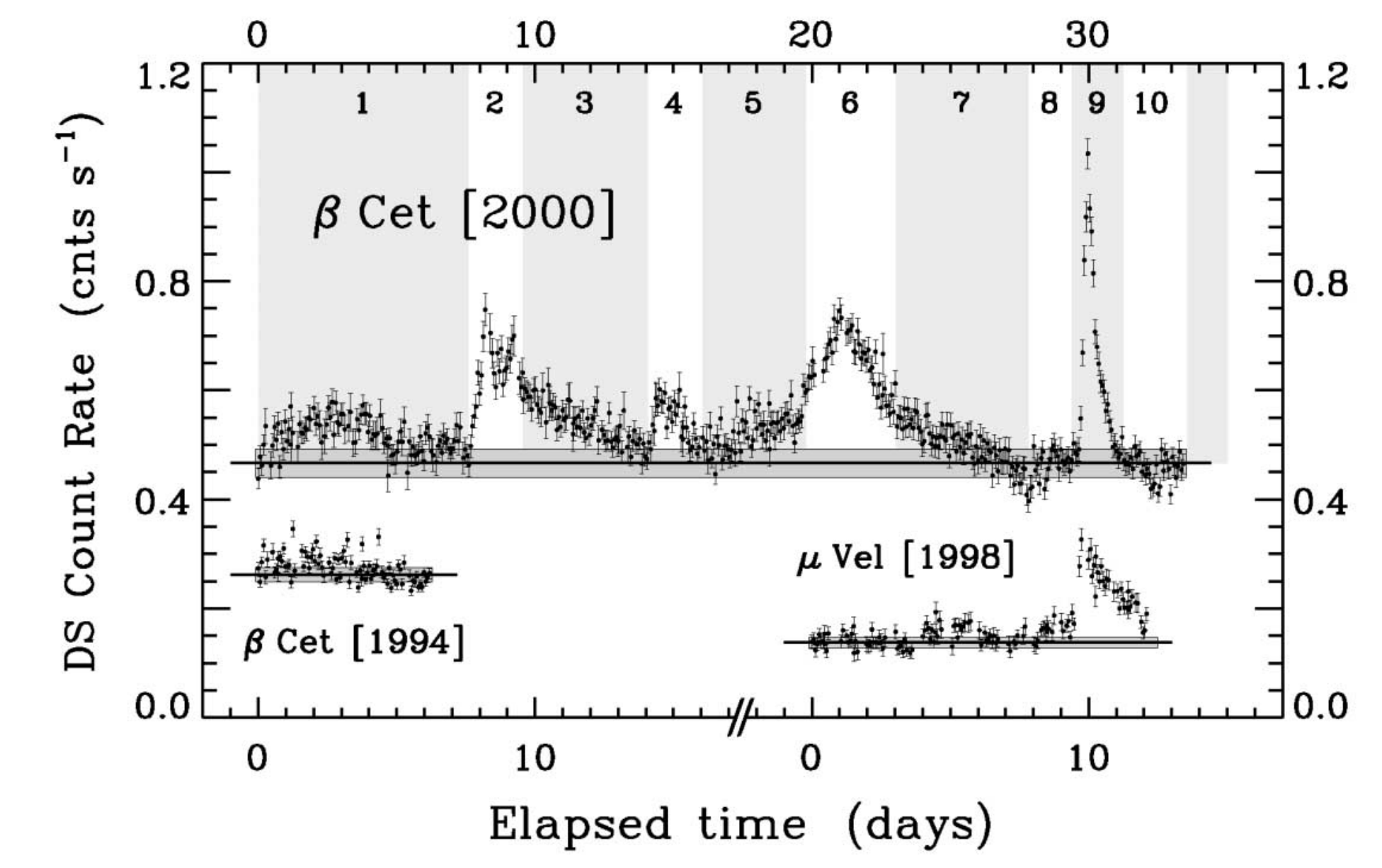
Figure 6: A small fraction of single, red clump giant stars like $\beta$ Ceti exhibit continuous variability that consists of week-long, giant EUV ($60-180$ Å) flares. A flare on $\mu$ Velorum (also shown) is even more unexpected in its evolutionary stage. Figure reproduced from [47] with permission.

5 Flare Rates and Flare Frequency Distributions

The rates at which stars flare have been measured through continuous ground-based observations, continuous space-based observations, and coarse sampling with serendipitous detections. The coarse sampling may result in just one data point per flare; thus an accurate characterization of the flaring source (Sect. 4) is often desired through follow-up spectroscopy. The study of flare rates is important for a wide variety of wider applications, including coronal heating physics [341], characterizing serendipitous variability in time-domain and exoplanet surveys [58, 768, 314, 65, 260, 305, 244, 507, 333, 124, 362, 636, 398, 764, 784], and studying the effects on exoplanet environments [e.g., 332, 713]. Much knowledge of stellar flares from low-mass stars is a result of monitoring a handful of nearby dMe stars, which reliably flare at a high rate. Large etendue time-domain capabilities of wide-field surveys such as the Sloan Digital Sky Survey, 2MASS, and ASAS-SN have been leveraged to characterize flare rates of inactive and early-type M dwarfs [411], at infrared wavelengths [156], and of ultracool dwarfs [655, 656, 657].

5.1 Basic Methods and Early Studies

[314] distinguish among flare rates, flare duty cycles (flaring fractions), and flare frequency distributions. Here, we focus on flare frequency distributions (FFDs), which refer to the energy dependence of the flare rates from continuous monitoring. Flaring fractions in sparsely sampled data are discussed in Section 5.3.

The seminal study of [433] presented an extensive flare rate analysis of several nearby active M dwarf (dMe) stars from hundreds of hours of ground-based monitoring in typical Johnson bandpasses. The high-time resolution data and observational details, along with some fundamental measurements such as equivalent durations, timescales, and peak amplitudes, can be found in [506]. In this section, we first present several basic measurements that are derived from flare light curves. The most fundamental calculation is the equivalent duration of a flare through a bandpass. The equivalent duration of a flare is the time that a star must spend in quiescence to produce the same energy as in the flare. It is a proxy of the flare energy, which is spectral type and luminosity class dependent, but can be readily obtained from relative photometry. The equivalent duration is [254]:

$$ED=\int_{t_{\rm{start}}}^{t_{\rm{end}}}{\frac{I(t)-I_{q}}{I_{q}}}\,dt=\int_{t_{\rm{start}}}^{t_{\rm{end}}}{I_{f}(t)}\,dt$$ (4)

which has units of time and requires establishing flare start and end times. A small equivalent duration can result from a small flare energy and/or a large quiescent count flux ($I_{q}$) at Earth. Note that the symbol for intensity, $I$, is traditionally used, though this quantity is actually the spatially unresolved instrumental ($I$) count flux from the star. The equivalent duration is multiplied by quiescent luminosity through this bandpass to obtain the absolute flare energy.

The integrand of the equivalent duration is known as the “flare visibility” or “flare contrast” and is denoted as $I_{f}(t)$. The flux enhancement relative to the flare star’s quiescence is known as $I_{f}(t)+1$ (Sect. 2). The numerator in the integrand is the “flare excess”, which can be denoted using a prime symbol to indicate a change. If the average flux is calculated from a continuum or pseudo-continuum region of a spectrum, then the flare-only flux is denoted as C$\lambda_{c}^{\prime}$, where $\lambda_{c}$ is a representative wavelength within the spectral window. The $I$ quantity is formally the count flux of the flare star normalized to the count flux from a nearby non-variable star ($I(t)=C_{\mathrm{rel}}(t)$ in Eq. 1) in the same exposure and same aperture radius. For a photon-counting instrument, such as a CCD, the theoretical value of $I$ is

$$I(t)=\frac{\int{T(\lambda)f_{\lambda}(\lambda,t)\lambda\,d\lambda}}{\int{T(\lambda)f_{\lambda,0}(\lambda)\lambda\,d\lambda}}$$ (5)

where $T(\lambda)$ is the total system response or effective area, including filter, atmospheric transmission (if applicable), and the detector gain; $f_{\lambda,0}$ is the flux spectrum of a comparison (non-variable) star or stars, and $f_{\lambda}$ is the flux spectrum of the target star in units in erg cm^-2 s^-1 Å^-1. The ED is then multiplied by the bandpass ($T$) quiescent luminosity ($L_{q,T}$) to find the bandpass-integrated flare energy, $E_{T}=ED\times L_{q,T}$. For known and well-characterized bandpasses, these can be determined using zeropoint fluxes, $f_{\rm{ZP}}$ [773] and published apparent magnitudes , $m_{T}$, at low-levels of flare activity:

$$m_{T}=-2.5\,\log_{10}\frac{\langle f_{q,\lambda}\rangle_{T}}{f_{\mathrm{ZP},T}}$$ (6)

where the zeropoint flux in the Vega mag system is determined by the numerical integration of a bandpass over the spectrum of the A0 V spectrophotometric standard star, Vega. If a flux-calibrated quiescent spectrum of the flare star is available, numerical integration over the total system response, $T(\lambda)$, including bandpass, alternatively yields the following:

$$L_{q,T}=\langle f_{q,\lambda}\rangle_{T}\,\Delta\lambda\,4\pi d^{2}=\frac{\int{T(\lambda)f_{q,\lambda}(\lambda)\lambda}\,d\lambda}{\int{T(\lambda)\lambda}\,d\lambda}\Delta\lambda\,4\pi d^{2},$$ (7)

where $\langle{f_{q,\lambda}}\rangle_{T}$ is the system-weighted flux [683], $f_{q,\lambda}(\lambda$) is the quiescent stellar spectrum at Earth in units of erg cm^-2 s^-1 Å^-1, and $d$ is the distance to the star. The width of the bandpass, $\Delta\lambda$, is usually taken to be the FWHM or the effective width, which vary from $\Delta\lambda\approx 600$ Å to $4000$ Å, for the SDSS $u$-band and Kepler bands, respectively. In recent years, quasi-bolometric conversions from white-light filters have assumed a blackbody function for all flares, and all phases of flares [e.g., 675]. Other studies assume constant spectral energy distributions, with energies reported over the limits of the bandpass [e.g., 304]. Several quiescent luminosities used for M dwarfs are given in Table 16 by [506], but it should be noted that stars, especially active M dwarfs, have a rather large spread of $U$-band magnitudes reported in the literature (e.g., reported quiescent apparent $U$-band magnitudes for the flare star YZ CMi range between $13.70-13.85$). Total system response characteristics through $U$ bandpasses are also inherently uncertain [e.g. 477] and to some extent, intractable. Thus, non-negligible systematic uncertainties in absolute energies are to be expected from a combination of these various issues [see 313, for empirical comparisons of flare energies in SDSS $u$ and Johnson $U$ from two different telescopes]. In Appendix A, we show several of the broadband and narrowband filters that are commonly employed in optical stellar flare studies.

FFDs are presented as either downward cumulative, $Q(>E)$, or differential, $n(E)$, distributions in log₁₀-log₁₀ space [see 39, for comparisons of these methods]. The most common practice is to fit a power-law (pareto) model to the unbinned, downward cumulative FFD:

$$Q(>E)=N\big{(}\frac{E}{E_{0}}\big{)}^{\beta}$$ (8)

with power-law index, $\beta$, and $N$ total flares greater than or equal to a fiducial low-energy limit, $E_{0}$ (e.g., the detection completeness limit) observed within a monitoring duration of $\Delta t$ (hr). The usual convention is that $\beta$ is negative. The differential FFD (# of flares per unit energy) is then

$$n(E)=-\frac{dQ}{dE}=N\frac{\alpha-1}{E_{0}}\big{(}\frac{E}{E_{0}}\big{)}^{-\alpha}$$ (9)

where $\beta=1-\alpha$ (again, the convention is that $\beta$ is negative and $\alpha$ is positive). Note that if $A\int_{E_{0}}^{\infty}n(E)dE=1$ is solved for $A$, the converted differential distribution $A\ n(E)$ is a probability density function (PDF): given a flare occurred, $A\ n(E)dE$ is the probability for a flare to have an energy between $E$ and $E+dE$.

Convenient analytic forms exist for the power-law index and its statistical uncertainty from a direct (i.e., unbinned) maximum likelihood (ML) analysis [757, 133, Appendix B]:

$$\hat{\beta}_{\text{ML}}=\frac{N}{\sum_{i=1}^{N}ln\frac{E_{i}}{E_{0}}}$$ (10)

from which the result follows that $\sigma_{\hat{\beta}_{\text{ML}}}\approx\hat{\beta}_{\text{ML}}/\sqrt{N}$.

Alternatively, weighted least-squares fits of the power-law index (slope) and intercept of a line in log-log space has been sometimes employed in stellar flare studies. For example, [433] express the power-law for each flare star in their sample of active M dwarfs as

$$\log_{10}\nu(>E)=a+\beta\,\log_{10}\,E$$ (11)

where $\nu(>E)=Q(>E)/\Delta t$ is the number of flares per hour greater than or equal to energy $E$ (expressed in erg) through an optical bandpass $T$. (To increase statistical confidence, flares that are observed in several bandpasses were multiply-counted using empirical bandpass energy conversions with the effective observing time adjusted accordingly.) Of course, the counts in even well-populated cumulative distributions have statistical uncertainties that are asymmetric in logarithmic space, and the values in cumulative distributions are non-independent. Nevertheless, this method is employed as a sufficient approximation in some cases given the statistics that are possible with the relatively low number of flares in ground-based observing campaigns.

Power-laws are typically fit to FFDs over an intermediate range of energy that is carefully chosen [e.g., 679] to exclude the high-energy and low-energy ends, which may have incomplete sampling that can affect the fits. Note that [133] present more sophisticated methods for uncertainty estimation for power-laws and have been employed in some more recent flare rate studies [496]. The Markov Chain Monte Carlo approach is described in [159], and [160] use an appropriate uncertainty analysis for the counts [253]. Modifications to the basic power-law form (Eq. 11) and completeness functions have been used to make adjustments to the the low-energy end [638, 27, 156, 496, 555] and high-energy tail [30] of FFDs. For reference, solar flare frequency distributions [136] exhibit power-law indices in (nonthermal) hard X-ray energy of $\approx 1.5$ and peak luminosity of $\approx 1.7$ [143], whereas the thermal soft X-ray peak flux exhibits a larger power-law index of 2.0 [738, 29, 339].

We summarize the general range of values of $\alpha$ calculated from FFDs in the X-ray and the optical regimes. Ground-based optical and space-based XEUV ($0.01-10$ keV, which corresponds to $1.24-1240$ Å, and where only EUV data, such as DS count rates, are available, a two-temperature, $T=6+23$ MK, optically thin free-free model extrapolates to the full XEUV range to calculate energies) flare rates have generally given values from $\alpha\approx 1.4-2.2$ with statistical uncertainties of $\gtrsim 0.1$ [39]. RS CVn systems exhibit power-law indices in the EUV on the lower end of this distribution [561]. [783] summarize the power-laws from 77 G-type stars. [304] and [351] summarize values of $\alpha$ for low-mass stars in the optical, and [464] present power-laws for low-mass stars of different activity levels in the FUV. A useful document that summarizes flare rates from low mass M stars of various spectral types is Osten (2016). Among the active M dwarfs, the higher luminosity stars (in quiescence) exhibit flatter power-laws [590], and thus the sum of the energy in all flares is dominated by the occurrence of the highest-energy flares [433]. Alternatives to the power-law functional form (Eq 9) are summarized in [25], [638], and [646].

A few stars have had power-law indices measured independently several times; these stars show some interesting systematic differences in the reported power-law properties. In the M dwarf study of [433], the famous flare star AD Leo appeared to be an outlier from the others. Due to the relatively short observing time in the [433], its FFD was recalculated after more data were collected. [590] found a value of $\alpha=1.62\pm 0.09$ from 85 $U$-band flare events (with 115 individual flare peaks) in 111 hr of monitoring. The most energetic flare was $10^{33}$ erg. The $U$-band FFD of Proxima Centauri has been quantified by [754] for flare energies between $5\times 10^{27}$ erg and $10^{30}$ erg, giving a similar value of $\alpha\approx 1.7$ to AD Leo but flatter than other stars of the same quiescent luminosity, such as CN Leo. Recently, [159] doubled the number of flares in the statistics for Prox Cen using white-light optical data from the MOST satellite and calculated a similar power-law slope to [754]. [332] found a steeper power-law for Proxima Centauri from the Evryscope survey and investigated the effect on the power-law index with and without an extreme superflare outlier.

[433] and [590] found trends in power-law indices with effective temperature or quiescent $U$-band luminosity: larger luminosity (earlier-type) main-sequence stars exhibiting flatter power-laws (i.e., smaller $\alpha$, $\mid\beta\mid$). However, the study of [590] did not include the results of [754] for the interesting case of Proxima Centauri, which shows a flatter power-law than expected; evidence for and against Proxima Centauri being less magnetically active than others of the same sub-type, such as CN Leo, are summarized in [620]. [39] suggested that $\alpha$ derived from the XEUV may exhibit an opposite trend with spectral type, though this is reported with low confidence. They find an increasing rate of $E>10^{32}$ erg flares corresponds with greater quiescent X-ray luminosity.

Other interesting quantities that have been calculated from flare star monitoring are the energy per flare (average flare energy) and the radiated flare energy per unit time (average luminosity due to flaring). These quantities are usually calculated through the $U$ band. They correlate with the non-flaring, bandpass quiescent luminosity [433] or non-flaring, bolometric luminosity of the star over several orders of magnitude. It should be noted that the number of detectable flares is anti-correlated with the quiescent luminosity, an effect largely due to brighter stellar background that raises the detection limit [e.g., 156]. Nonetheless, including many small, unobserved flares in the total energy calculation does not change the trends. From modern space-based data, it seems that these relationships generally extend to active binaries, which comprise much higher luminosity stellar components [570]. An extrapolation of these relationships to the Sun, however, dramatically over-predicts the flare energy release rate in optical solar flares by many orders of magnitude, as first noted by [433]. From Kepler data (Sect. 5.2), a somewhat similar quantity of $L_{f}$ vs. $L_{\rm{Kp}}$ has been constructed by [466] and is making for powerful comparisons for normalized flaring efficiencies among stars of different spectral types [e.g., 160]. Davenport [155] investigates evidence for saturation in the relative flare luminosity given by $L_{f}/L_{\rm{Kp}}$ at small Rossby numbers, analogous to the quiescent $L_{X}/L_{\rm{bol}}$ saturation (Section 4).

There has been a severe paucity of low-activity M dwarf flare rates until [304] presented white-light 1-minute cadence data from Kepler and some previously unpublished ground-based $U$-band data from the PhD work within [313]. These studies revealed that stars that are optically inactive in quiescence (Sect. 4) produce broadband optical flares, a result that had been quantified in sparsely sampled data from the Sloan Digital Sky Survey [411] and from serendipitous spectral detections [579]. [464] compared FUV flare energies among stars with comparable quiescent bolometric luminosities and found that FFDs are shifted according to the quiescent flux in the FUV.

The different apparent behaviors at the high-energy ends of stellar flare FFDs are still largely unexplained. Does the power-law that is well-fit to a middle range of energies continue on indefinitely, or does it turn over at the high-energy end and follow a steeper power-law index [176, 570] or another type of roll-over [e.g., 566, 149, 30, 136, 646] for some stars? What physical parameters determine the upper limits of flare energies (and peak luminosities) that are possible on a given star? Extending the power-law that is fit to the FFD of YZ CMi predicts a $U$-band flare to occur about once per month with an energy that is a factor of $5000-10,000$ larger than its mean flare energy [433, 412]. Dal and Evren [152] discuss an upper limit to the energy released in dMe flares is approached as the flares become longer in total duration. Shibata et al [674] and Aulanier et al [41] present theoretical grounds and semi-empirical relations for upper limits of flare energies. Empirical constraints from very long monitoring times have only been possible recently using Kepler data.

5.2 White-Light Flare Rates & Kepler

The release of Kepler data [80] has transformed knowledge of flare rate statistics in several important ways. First, the high precision and long monitoring times facilitate detection of relatively rare white-light flares from older, less active low-mass stars, from much larger luminosity stars such as solar-type stars, and from higher mass K and early-type M dwarf stars, and evolved stars. Second, it provided many more hours of monitoring per star: ground-based monitoring efforts resulted in $\approx 30-100$ hours per star, while the nominal baseline for Kepler was two contiguous months of observations per star. The flare statistics correspondingly improved, but the high precision also revealed comparable amounts of background flux variation due to starspots and rotation. Nonetheless, the Kepler field began as a relatively poorly known star field (due to its relatively faint magnitude limits), and systematic contamination of the flare sources from binaries, subgiants, and other non-flare sources was an issue until targeted, ground-based spectroscopic (and asteroseismic) analyses caught up and Gaia DR2 parallaxes became available. Additionally, the vast majority of data from the Kepler mission is at 30-minute cadence, and most superflares span just two to four data points. The 1-minute cadence data were made possible for select stars through Guest Observer programs [e.g., 304].

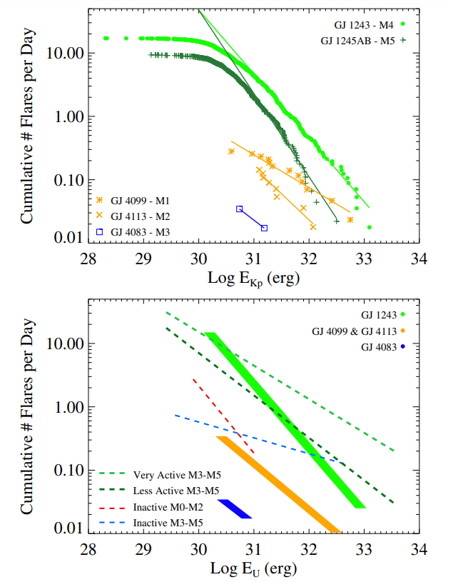
Figure 7: Flare frequency distributions of several main-sequence M stars in the Kepler band (top) and in the $U$-band (bottom). Figure reproduced from [304] with permission. Note the spread in flare rates in the bottom panel among the very active and less active stars of the same spectral types.

The dM4e star GJ 1243 has been observed for 11 months at 1-minute cadence with Kepler, making it the longest observed flare star in the sky besides the Sun. The FFDs and flare properties of this star have been studied extensively by [604, 304, 157, 155, 679]. From the database of over 6000 flares, [679] obtained a value of $\alpha=2.008\pm 0.002$, and [161] inferred $\alpha=1.942\pm 0.001$. From the first two months of data, [304] found $\alpha=2.01$. They also noted that the turnover in the FFD at the low-energy end, which has often been attributed to a detection limit effect, may be astrophysical at some level since flares of these energies should be readily detectable above the precision of Kepler. The FFD of GJ 1243 is shown in Fig. 7(top) in comparison to several other M dwarfs spanning different spectral types and levels of quiescent magnetic activity (dM v. dMe). Comparable diagrams with compilations of FFDs of many individual stars are shown in [668], [604], and [149]. [466] presented a detailed analysis of the GJ 1243 AB system, where they separated the Kepler light into the two stellar components and found values of $\alpha\approx 2$ for both stars, but a higher flare rate occurs on the slower rotator. The bottom panel of Fig. 7 shows the Kepler energies converted to energies in the $U$-bandpass. The flare rates of “less-active” M3–M5 stars are closer to the FFD of GJ 1243, whereas the very-active M3-M5 stars include the dMe stars from [433], such as YZ CMi, EV Lac, and AD Leo. A continuum of flare rates is clearly evident as the vertical offsets of the power-laws, while different power-law slopes may be a result of vast differences in statistics from ground and space-based monitoring [304].

The spread in flare rates among active M-dwarfs of similar spectral types (Fig. 7) contrasts with the findings of [411], who found that the average M4Ve-M5Ve flare frequency distribution from sparsely sampled data of field stars in the Sloan Digital Sky Survey (SDSS) Stripe 82 is sensibly in line with that of the well-known flare star YZ CMi (which is one of those among the “more active” stars in Fig. 7). [313] began to investigate the chance alignment of FFDs in [411] using Monte Carlo sampling of simulated flares at the SDSS $riuzg$ cadence. The resolution of this issue (which is a non-trivial adjustment to the statistical rate calculation; E. Hilton, priv. communication 2013) will be important for accurately mapping flare rates of the Galaxy using sparsely sampled data from the LSST [358].

The immaculate flare statistics of Kepler facilitated new timing analyses of flare occurrence and correlation. The flare occurrence of GJ 1243 was investigated as a function of the phase of the longer-timescale, flux modulation that exhibits a $\approx 1$% amplitude and is attributed to stellar rotation. No significant correlation was found at either maximum or minimum flux levels. The relationship between flare occurrence and phase was further investigated in detail with larger samples of flares on GJ 1243 [679] and for a large sample of M dwarfs [466, 185]. Morris et al [515] reported a larger flare occurrence when the very low-mass (M8V) star TRAPPIST-1 is slightly brighter than average and when it goes through the increasing flux phase in the Kepler light curve. [151] investigated the occurrence of different types of flares with phase from a large sample of ground-based observations of flares.

[304] finds that the intervals between successive flares (“waiting times”) on an active M dwarf (GJ 1243) over many rotation periods is consistent with a single exponential probability distribution, $p(\Delta t_{\rm{next}};\tau_{0})$ $\propto\frac{1}{\tau_{0}}e^{-\Delta t_{\rm{next}}/\tau_{0}}$ (where $p$ is the probability density and $\tau_{0}$ is the average interval between consecutive flares). Equivalently, the number of flares occurring in fixed time intervals, $\Delta t$, is Poisson-distributed, $p(N_{\rm{flares}}$; $r,\Delta t)=(r\Delta t)^{N_{\rm{flares}}}e^{-r\Delta t}/(N_{\rm{flares}}!)$ [e.g., 433]. Stellar flares from active stars thus occur independently and continuously at a constant rate, $r=1/\tau_{0}$ (note that some studies use $\lambda$ instead of $r$ for the rate), except possibly on some short time-intervals ($\Delta t\lesssim 30$ min) within complex events [304, 157]. Correlations between waiting time and flare energy, as may be expected from magnetic energy buildup and release [e.g., 638] in a single region on the star, are not clearly consistent with the stellar data [304]. Efforts to understand the flare occurrence as a function of light-curve phase are ongoing in the era of TESS data [350].

[157] constructed a canonical flare template from the normalized, classical (single-peaked) flares of GJ 1243 in short-cadence Kepler data. They modeled the decay phase with a sum of two exponentials and the rise phase with a polynomial. The template reflects a remarkable self-similarity in many flares on one-minute integrations. Further analysis in this work demonstrated that many complex flares can be decomposed into linear superpositions of several templates with adjustable parameters. They then injected synthetic flares over a long time baseline and simulated flare statistics, concluding that the number of complex flares observed in the data is not fully consistent with a chance superposition of many uncorrelated classical flares. This is tantalizing, quantitative evidence for a solar-like “sympathetic” [e.g., 467] flaring property of stars.

The rates of flares in the high-energy regime have been investigated in detail with Kepler data. Silverberg et al [679] discuss a deviation from a single power-law between $E_{\rm{Kp}}=10^{32.5}-10^{34}$ erg flares in the GJ 1243 sample. (In the following, flare energies now refer to the energies integrated over a $T=9000$ K blackbody function, as reported in the respective studies, rather than an energy over a particular bandpass). The upper limit flare energy for white-light flares has been pretty well established from the long monitoring times from Kepler to be $E_{\rm{max}}\approx 10^{37}$ erg for subgiants, $E_{\rm{max}}\approx 10^{36}$ erg for rapidly rotating G-dwarfs, and $E_{\rm{max}}\approx 10^{35}$ erg for slower rotating G dwarfs [551, 555]. For G, K, and M stars in the Kepler field, Candelaresi et al [109] discuss a correlation between a star’s superflare ($E>5\times 10^{34}$ erg) rate and its light-curve amplitude modulation due to starspots. The ground-based Evryscope network has also provided new insights into $g^{\prime}$-band superflare rates: Howard et al [333] find that the rate of $E\geq 10^{33}$ erg superflares (by extrapolating the best-fit power-laws down over $0.5-1.5$ orders of magnitude in energy for the K5-M2 stars) decrease from the averaged active K5-K7 stars to the averaged active M4 stars. Similar to many previous studies (Section 5.1), they report a larger average flare energy for earlier-type stars, which they attribute to the “size of the stellar convective region”. Pettersen [588] review and analyze the time-averaged luminosity due to flaring (and quiescent magnetic activity proxies) in a sample of dKe and dMe stars, and they correlate it with the convective envelope volume. Recent stellar evolution models of dM flare stars in eclipsing binary systems [214, 215] and dK/dG stars [488] also show that early type stars, which have larger mean flare energies, have larger convective zone volumes.

5.3 Timing on Long Scales: Flare Rates and Stellar Age

By characterizing the FFDs across many types of stars in different evolutionary stages, astronomers begin to piece together how flare rates change over billions of years. With age-dating techniques such as open cluster membership / association and gyrochronology, quantitative evolutionary tracks in the flare history of stars are possible. At the youngest stellar ages, high flare rates and energies have been reported from PMS stars in nearby open clusters, such as Orion, in the X-ray and optical [256, 361]. Signatures of accretion (e.g., in T Tauri systems) indicate a very young age range for some flare stars [e.g., 715]. Membership among moving groups, such as the well-known $\beta$ Pic moving group (with the flare star members AU Mic and AT Mic AB) probe ages around $\sim$ 20 Myr for stars that are no longer actively accreting gaseous material from a circumstellar disk. At older ages ($\gtrsim 100$ Myr), flare rates and properties have been reported in open clusters, such as the Pleiades [695, 352]. At the oldest ages, globular cluster and the Galactic bulge membership facilitates calibration of the flare-rate–age relationship, but such stars are located at very large distances. As stars spin down due to angular momentum loss over their main sequence evolution, flare rates are expected to correspondingly decrease. This correlation is supported by detections of stellar superflares from main sequence, rapidly rotating (periods $<$ 5 d) G-type stars. However, binarity plays an important role in maintaining flaring among a population stars to old ages, compared to the Galactic disk populations. This may occur through a co-evolutionary process in M dwarf-white dwarf binaries [513] or rotational tidal synchronization in RS CVn-like systems [570]. Binarity may also directly affect flare occurrences and energies [e.g., 176, 250, 4, and see references in Section 7.5], but it is in general a difficult property to assess without adaptive optics [e.g., 132] and high-resolution spectroscopy [e.g., 547], which are observational techniques that are limited to nearby stars.

Following the statistical inference of quiescent magnetic activity lifetime analyses of [769], the vertical distances above or below the Galactic plane have been used as proxies of stellar age for M dwarf stars in the field. The basic idea is that over time, stars experience repeated gravitational scatterings in the midplane of the Galaxy and are consequently more likely to be found at larger vertical displacements. Large time-domain surveys, such as the SDSS and soon the LSST, allow characterization of flare rates in multiple populations of stars in sparsely sampled data sets. The stellar flaring fraction and the flare fraction (duty cycle) are two quantities that are useful in mapping the flare rate of a galaxy and the star’s vertical distance from the galactic plane. A stellar flaring fraction is the fraction of stars that produce some number of flares, while flaring fraction, or duty cycle, is the fraction of sparsely sampled epochs that flare. UV and optical surveys have been leveraged to map these quantities with increasing vertical distances [768, 411, 314, 756]. There is suggestive evidence that flaring fraction from sparsely sampled data indicates that flaring occurrence among a population decreases faster with stellar age than other measures of quiescent magnetic activity [411, 314]. One may be tempted to speculate that this is one possible source for the spread in flare rates among the mid-type dMe stars in Fig. 7, but more investigation is needed. The effects of solar-like activity cycles [143] might also sensibly contribute to the variation of flare rates within a population of stars of the same spectral type [but see 590, 161].

Most recently, the improved methods and data samples for flare statistics, asteroseismology, gyrochronology, and open cluster calibrations using Kepler and K2 data have facilitated much more quantitative characterization of the flare rate as a function of stellar age [e.g., 351, 352]. [160] used Kepler field stars and gyrochronology [479] to present the first stellar flaring fraction as a function of age and $g-i$ color, which maps to spectral type [138]. [160] used MCMC non-linear least squares to constrain $\alpha(t)$ in an equation similar to Eq. 11 over a range of stellar masses, from G to M dwarfs, and ages older than $t\geq 10$ Myr. They found that $\alpha(t)$ remains approximately constant, flare rates indeed decrease over time for the M dwarfs, but that the flare rate decreases much less than for the G dwarfs. [551] and [555] characterized the evolution of differential flare frequency of G-type stars in the Kepler field by splitting up into different rotational period bins from $<5$ d to $20-40$ d. They further divided the $<5$ d sample into smaller bins and found that flare frequency is approximately constant for periods $<$ 3 d, for which the corresponding ages are $\lesssim 500$ Myr but are not as well constrained from gyrochronology calibrations. Johnstone et al [368] combine several state-of-the-art techniques to calculate the quiescent $L_{X}$ as a function of age and mass, and then they leverage a scaling relation (discussed in Sect. 5.1) from Audard et al [39] to map the rate of high-energy XEUV flares on GKM stars over ages spanning 2 Myr to 5 Gyr.

6 Light Curve Analyses

In addition to integrated flare energy in a particular bandpass (Sect. 5), a number of other strictly empirical quantities can be calculated from single-bandpass data with a moderately fast cadence. A useful decay timescale measurement is the time it takes for a light curve to reach $1/e$ of its maximum flux [e.g., 473, 526], which prevents ambiguities in determining the bona-fide end of a flare. This measure also avoids model-dependent uncertainties in fitting an exponential function to flares with events in the decay phase, which may also show lengthening timescales [567, 157]. Here, we summarize a few relationships between decay times and other quantities. The total rise and total decay times of flares are not well-correlated [506, 433, 304], which possibly suggests some loss of “memory” about the details of the rise phase after the peak. Integrated energy and total duration exhibit a tighter correlation. Larger peak-flare amplitudes typically correspond to longer decay times and larger energy flares, but there is significant scatter. [526] find that the $1/e$ decay duration scales with total white-light energy to the $1/3$ power and magnetic field to the $-5/3$ power for flares on the Sun, rapidly rotating G stars [see also 473], and M stars [see also 333]. Kővári et al [390] found that the $1/3$ power scaling between duration and energy also extends to a late-type giant. For similar-duration ($\approx 5-10$ min) solar flares and white-light flares on solar-type stars, the energies of the latter are several orders of magnitude larger [cf Figures 8-9 of 526].

6.1 Classification of Flares by Optical Broadband Evolution

Several classification schemes of flares have been developed based on optical broadband durations and light curve shapes (“morphologies”). [78] and [506] established some of the basic descriptive terminology of flare classification, such as complex, spike, slow, typical, or multipeak (a type of complex flare). More recently, a condensed scheme denotes flares as either classical or complex [157]; several classical and complex events are evident throughout a small section of the Kepler data of GJ 1243 in Figure 8(top) panel. [420] argued that flares with several events that comprise the rise phase can appear as relatively simple, “classical” flares if degraded to 1-minute time-integrations. A classification of solar flares into “gradual”, “impulsive”, and “secondary” was proposed by [134] based on extremely high-time resolution, hard X-ray data. Hard X-ray data is rarely available for stellar flares, and impulsive and gradual classifications have thus been determined from broadband $U$- and optical light curves.

A common classification utilizes a measure of the impulsiveness (also referred to as “impulse” or “impulsivity”), of a flare. [297] quantified the impulsiveness as the fraction of energy emitted in the impulsive phase, which ends after the fast-decay phase(s) in broadband optical radiation. They found that about 70% of the energy was emitted in the impulsive phase during two flares that are separated by $\sim 2$ orders of magnitude in total energy. These were both considered very impulsive events. [413] classified three events as “gradual”, “impulsive”, and “traditional” in ultra-high-cadence (0.16 s) photometry data. [414] calculated the impulsiveness index ($\mathcal{I}$) as the peak value of $I_{f}$ divided by the FWHM ($t_{1/2}$) of the broadband ($U$) light curve to classify events into “impulsive flares (IF)”, “hybrid flares” (HF), and “gradual flares” (GF). Examples of high-energy, $E_{U}>10^{32}$ erg, GF and IF events are shown in Figure 8(middle). Lower-energy and lower-amplitude IF, HF, and GF events are shown on the same axes in the bottom panel of Figure 8. [150] divide a large sample of dMe flares into fast and slow flares and suggest the differences are related to the position on the stellar disk. This hypothesis could be verified with spectral properties that are thought to change with position on the solar disk [538].

The Kowalski et al [414] IF/HF/GF impulsiveness index is primarily a diagnostic of the broadband evolution during the impulsive phase of a flare. Thus, it is smaller for flares with a gradual decay phase that starts at a flux level that is a significant fraction of the peak flux. Among the IF-type events, there is a large range, $30-70$%, in the percentage of the total energy that is emitted in the impulsive phase. Several spectral quantities (Balmer jump ratios, Balmer line-to-continuum ratios; Sect. 7.2) at the time of peak broadband flux correlate with this index; one possible interpretation is that the average impulsive-phase heating rate varies among events. If the heating rate is attributed to the flux of electron beams, then the inter-flare variation of these optical spectral quantities suggests [416] an important connection between large-scale flare evolution and electron acceleration, which is sometimes discussed in the context of nonthermal hard X-ray properties of solar flares [492, 320]. This expands upon the foundational paradigm that stellar flare scaling relations (e.g., H$\gamma$ v. $U$-band energies), which extend over many orders of magnitude, mean that differences from flare to flare primarily result from the flaring surface area [e.g., 104, 297]. The empirical differences in IF/HF/GF spectra thus eventually motivated the semi-empirical modeling work in Kowalski [408], which suggests that differences among flares further result from scaling the relative areas of higher and lower concentrations of particle beams in the stellar atmosphere. Recent analyses of H$\alpha$ line profiles from different locations within solar flare ribbons have begun to quantitatively explore the implications for spatially unresolved stellar data [528].

The fraction of flares within each of the IF, HF, and GF types is not yet well-established. The reported numbers of flares that are IF/HF/GF [414] are biased toward the IF type because the larger signal-to-noise at peak facilitates spectral characterization. Note that rigorous distinctions cannot be made between an HF and GF classification for certain events [420]. It is also not clear how many IF events produce larger Balmer jumps [416] than expected according to the original [414] IF/HF/GF classification scheme. GF events in the decay phase of highly-impulsive events also have shown some of the smallest Balmer jumps (in absorption).

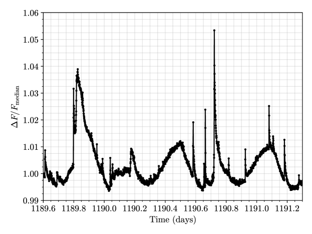
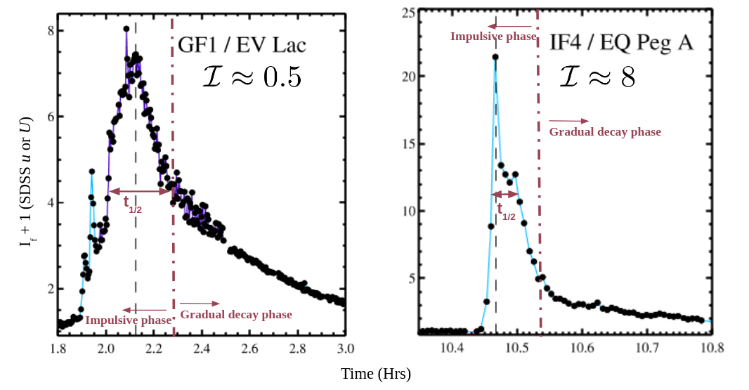
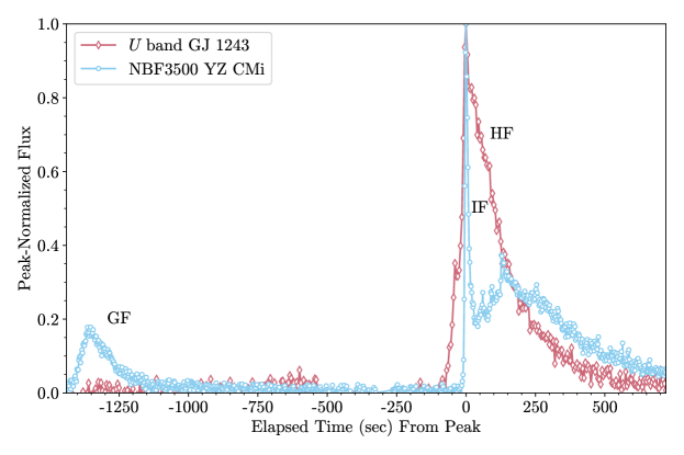
Figure 8: Representative high-cadence optical light curves of M Ve flares. (Top) A randomly chosen section of the 1-minute cadence Kepler light curve of GJ 1243 from [157] showing a variety of classical and complex flares superimposed on the modulation, which is due to starspots [158]. The data were obtained from https://github.com/jradavenport/GJ1243-Flares. Note, there was a single flare event (not shown) that was observed simultaneously in both Kepler and in the $U$-band [304]. For reference, this flare had a relative peak contrast of $\Delta F/F_{\rm{median}}=0.014$ in the Kepler band, a peak contrast of $I_{f}=0.9$ in the $U$ band, and a total $U$-band energy of $10^{31}$ erg. (Middle left) The impulsive and gradual decay phases of a high-energy gradual flare (GF) event on EV Lac; reproduced with permission from [414]. The impulsive phase and gradual decay phases are indicated. At the peak (vertical black dashed line), GF-type events like this one have large Balmer jumps, which are still much smaller than predicted by optically thin hydrogen recombination theory alone (e.g., Sect. 7.2.1). The $t_{1/2}=13$ min is the FWHM of the light curve, and the $U$-band impulsiveness index, $\mathcal{I}=I_{f}/t_{1/2}$, is 0.5 for this flare. (Middle right) An example high-energy IF event ($t_{1/2}=2.5$ min, $\mathcal{I}=8.3$) on EQ Peg A, reproduced with permission from Kowalski et al [414]. (Bottom) Examples of lower energy flares within the flare IF/HF/GF classification scheme based on the impulsiveness in the $U$-band or a narrow-band filter (NBF) with $\lambda_{c}=3500$Å. The HF and IF events have similar peak contrasts ($I_{f}=2.7-3.7$) but differ significantly in the values of $t_{1/2}$ (14 s and 120 s). The IF and GF events are referred to as IF4 and GF2 in Kowalski et al [416]; the HF event is referred as the HST-2 flare in Kowalski et al [420]. Note, the flare-only impulsive-phase spectrum of the IF event is shown in comparison to common photometry filters in Appendix A.

Nonetheless, it is rather clear that the most gradual-type events in the light-curve evolution exhibit the largest Balmer jumps ratios and ratios of H$\gamma$ / C4170^′ at the peak time in broadband optical flux, whereas the most impulsive-type events show the smallest Balmer jumps in emission and the largest fraction of optical energy that is radiated in the continuum (Sect. 7.1). This is possibly an interesting connection to the Type I and Type II white-light flare classification on the Sun (Sect. 7.2), but the stellar events that would, ostensibly, be most analogous to Type II white-light flares in the spectral properties are actually the stellar events that are most impulsive.

We should clarify that an impulsive-type flare exhibits an impulsive phase and a distinct gradual decay phase, while a gradual-type flare can show a gradual decay phase that is clearly distinct from its impulsive phase. Figure 8 (middle left) shows an energetic, gradual-type flare event that exhibits several faster impulsive events superimposed on a more gradual rise phase; the impulsive phase of this GF event ends around $t=2.3$ hrs and transitions to a more gradually decaying phase.

6.2 Quasi-Periodic Pulsations

High-time resolution data of stellar flares facilitate searches for periodicity over the light curve evolution. Some events have shown fluctuations in the broadband flux having periods with a modulated amplitude or an evolving period over a cycle or two; these are called quasi-periodic pulsations (QPPs). This topic is of significant interest within the solar and stellar communities [749], but an exhaustive discussion and reference list are outside the scope of this review. I summarize a few selected results. For detailed discussions and recent reviews, see [91] and [801].

QPPs in stellar flares are reported on a variety of timescales, from 10 s to 30 minutes, and they occur in the impulsive and gradual phases. [487] report a 10 s period during the $u$-band flare in the peak phase using a wavelet analysis [719] and discuss different interpretations, including one in which the reconnection and particle acceleration are modulated through MHD oscillations in a nearby large loop [525]. [16] detect a damped 32 minute oscillation during the decay phase of a $U$-band megaflare [412] on YZ CMi using Lomb-Scargle and autocorrelation analyses of the detrended light curve. Doyle et al [184] discuss shorter, $1-4$ minute, QPPs in two giant ($E\approx 5-10\times 10^{33}$ erg) flares observed on YZ CMi with $0.25-0.6$ s sampling. The AFINO method [353, 354] is another powerful technique for evaluating the statistical significance of QPPs. [353] apply the AFINO method to the stellar event in [16] and Kowalski et al [412] using a Fourier power-spectrum analysis that includes the component of the flare signal that is detrended in the wavelet technique. This approach accounts for the fact that some types of power-spectra may naturally give rise to types of bursty light curve behavior in the temporal domain.

Stellar flare QPPs are reported in data from the optical to the X-ray regimes on a wide variety of stars. Cho et al [129] investigate a tight correlation between the damping times and periods of QPPs in a sample of X-ray stellar flares. White-light QPPs in Kepler data are presented in [50]. [486] report remarkable oscillations with a 240 s period during the peak phase of a $U$-band flare on the RS CVn II Peg, and [504] discuss several physical origins in the damped 750 s period in the X-ray flare on the lower-mass system AT Mic. For an analysis of multi-band data during the decay phase of an X-ray flare on the young G star EK Dra, see [92]. QPPs of 320 s and 660 s periods were reported over the peak phase of a remarkably energetic flare on a PMS M3 star [360].

7 Multi-Wavelength Spectral Observations

Multi-wavelength observations of stellar flares are grouped into categories according to the regions of the atmosphere producing the electromagnetic response. A predominantly thermal response in the optical and near-ultraviolet originates from the cool, $T\approx 10^{4}$ K, dense lower atmosphere (Sect. 7.1 – 7.2), while the far-ultraviolet emission lines probe the rapid response of transition region temperatures around $T\approx 10^{5}$ K (Section 7.3). Nonthermal radiation originates from accelerated particles gyrating in coronal magnetic fields (Sect. 7.4 – 7.5), and a thermal response results from the hot, $T\gtrsim 10^{7}$ K, tenuous upper atmosphere (Sect. 7.6). The temporal correlations (Sect. 7.7) among these radiative responses justify a solar-like modeling paradigm with nonthermal electron beams and chromospheric evaporation and condensation processes (Sects. 3 and 8.2).

7.1 NUV and Optical: The Thermal Radiative Response of the Footpoints to Impulsive Nonthermal Heating from Above

The optical and NUV response is one of the most enigmatic and energetic aspects of stellar flares. This phenomenon is known for its dramatic impulsive phase, but it also exhibits a long-duration gradual decay phase that can extend for many hours after a bright peak flux phase. Long-duration continuum flare radiation may persist after relatively small peaks as well [see the GF1 event in Kowalski et al 414 reproduced in the middle left panel of Fig. 8 and the event studied in 298]. The optical and NUV radiation is thought to be thermal radiation that originates from photospheric and/or chromospheric heights. For reference, Table 7 summarizes several of the largest broadband optical flux enhancements in well-studied MVe flares with multi-band photometry data that include the $U$- or SDSS $u$-band.

Table 7: Flux enhancements at peak phase for several especially large MVe events with simultaneous multi-band photometry. The flux enhancement values ($I_{f}+1$; Sect. 2) are reported relative to the pre-flare or quiescence in each band. The flux enhancements are related to magnitude changes through Equation 1.

(row) Star	SpT	$E_{U/u}$ (erg)	$U$	$u$	$B$	$g$	$V$	$r$	$R$	$I$	$i$	3500†	4170†	6010†
(1a) YZ CMi	M4.5Ve	$\approx 4\times 10^{33}$										30.9	7.6	1.7
(1b) YZ CMi	M4.5Ve	$\approx 4\times 10^{33}$										106	28.7	3.8
(2) YZ CMi	M4.5Ve	$1.85\times 10^{33}$		78.2		6.3		2.6			1.35
(3) AU Mic	M1(V)e	$1.6\times 10^{33}$	3.4				1.13
(4) AD Leo	M3Ve	$6.5\times 10^{33}$	70		11		3.4		1.6
(5) EV Lac	M3.5Ve	$3.9\times 10^{32}$	40	40		4
(6) EV Lac	M3.5Ve	$6.2\times 10^{32}$	8.0	7.4		1.4		1.18
(7) SDSS J001309	M6Ve	…		158		16.9		8.6			2.0

7.1.1 Overview of Emission Line Properties

An overview of the temporal response of various emission lines and continuum fluxes in the $U$ band and optical regimes throughout a high-energy flare ($E_{u}>10^{33}$ erg; Table 7) is shown in Fig. 9. The temporal sequence in the figure is representative of many stellar flares, although quantitative differences among events occur [329, 327, 414, 420]. The line fluxes respond rapidly in the impulsive phase, except that Ca II K (and H) peak well into the gradual decay phase of the optical flare continuum flux. The late peak of Ca II K is a remarkable phenomenon in stellar flares [297, 330, 327, 251, 414]. The blue continuum flux is the fastest to rise to its maximum and then begin its decay, followed by the highest order Balmer lines [297]. The Balmer H$\alpha$ line is the slowest to decay relative to its peak [see also 527]. In some flares, the Balmer line peaks occur significantly after the peak of the continuum, which may be empirically related to secondary events [e.g., 297, 251, and see also the IF4/F2 event in Kowalski et al 416]. The neutral helium lines exhibit a very wide range of decay timescales: The blue He I lines decay quickly [297], but He I 10830 Å  (studied in a different MVe flare) exhibits one of the most gradually evolving light curves [654].

Quantitative assessments of the time-scales of emission line and continuum fluxes have been investigated with a time-decrement [414, 420]. The time-decrement is defined as the empirical trend of the full-width-at-half-maximum ($t_{1/2}$) of each light curve, plotted as a function of the wavelength of the transition. Are the relative decay timescales in Fig. 9 consistent with a simple model consisting of a slowly decreasing average temperature over the flare footpoints on the star [289, 329]? This explanation would be analogous to the cooling thermal loop sequence in solar flares [28] that is attributed to the temporal offsets in the maximum of optically thin, XEUV light curves. The average temperature properties of the flare region are undoubtedly important in understanding stellar flare light curve evolution in Fig. 9. However, the ratios of the Balmer line fluxes (which is called the Balmer flux decrement, or just “Balmer decrement”) and line-to-continuum flux ratios in the observations suggest that chromospheric optical depths [428, 193], vertical and transverse spatial inhomogeneities [415, 408], and non-LTE radiative transfer [295, 9] are probably also critical to interpret the sustained chromospheric emission line fluxes (and the relative evolution of the optical continuum fluxes) in stellar flares. In summary, there are not yet any comprehensive physical models that explain the absolute and relative timescales of the various optical spectral variations in Fig. 9.

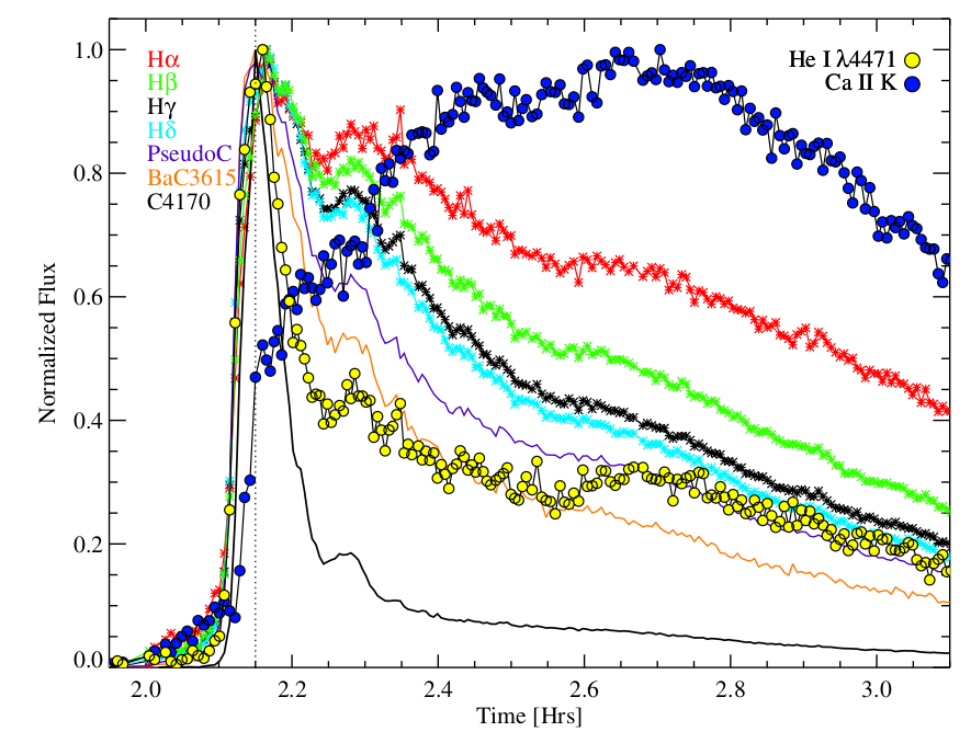
Figure 9: Representative time-evolution of optical spectral quantities over a giant flare on the M4.5Ve star, YZ CMi. The peak optical broadband magnitude enhancements are listed in row (2) of Table 7. The emission line fluxes are integrated over wavelength, and all light curves are normalized to their respective peak fluxes. The C4170^′ light curve is a proxy for the flare-only blue continuum flux averaged over $\lambda=4155-4185$ Å and is the fastest to decay after its peak flux is attained. The H$\alpha$ and Ca II K emission lines are the slowest. Figure reproduced from [414] with permission.

7.2 Spectral Properties of the Optical and NUV Continuum Radiation

The continuum fluxes through the NUV and optical are clearly much more impulsive than the emission lines in Fig. 9 (see also [297, 251, 420]). The observed flare continuum radiation from the NUV through the optical is collectively referred to as the white-light. In this review, we adopt the empirical definition (without regard to its origin in the stellar atmosphere) that a white-light flare is a broad-wavelength increase in the observed NUV, $U$-band, and optical continuum stellar flare radiation that sometimes extends into the FUV and NIR. Thus, the white light would contribute a majority of the integrated flux in optical broadband filters (e.g., $UBVR$, Kepler, TESS).

In this section, we review observational properties of optical and NUV flare continuum radiation, as revealed by spectroscopic measurements. We separately discuss peak/impulsive phase spectra (Sect. 7.2.1) and gradual decay phase spectra (Sect. 7.2.2). In Sect. 7.2.4 and Sect. 8.2, we review some closely-related results from analyses of colors in broadband photometry (“colorimetry”). The M-dwarf flare spectral observations, combined with detailed modeling, suggest that there are unexpected amounts of heating over a large (deep) column mass density (hereafter, just “column mass” or $m_{c}$; g cm^-2). Whether the $\lambda=1300-9000$ Å continuum radiation in stellar flares is caused by heating the photosphere to bona-fide incandescence (i.e., isotropic blackbody radiation or a blackbody-like spectral intensity) is an open question that is discussed in the next section and further in Sect. 8.2. The data discussed in this review come mostly from dMe flares, which produce large contrasts against their non-flaring photospheric radiative fluxes at blue and optical wavelengths. This property facilitates isolating “flare-only” spectra, which can be readily compared to models without the ambiguities of subtraction artifacts.

7.2.1 Rise and Peak Phase

A commonly reported empirical property of the optical, $\lambda\geq 4000$ Å, flare-only continuum radiation in the spectra of the impulsive phase of stellar flares is a color temperature matching a $T\approx 8,000-14,000$ K blackbody [505, 297, 380, 579, 414, 265, 434, 416]. The blackbody color temperatures might be purely phenomenological, in which case the color temperature values are parametrizations of the spectral shapes rather than analogs to in situ “thermometer readings” (Appendix C.1). A temperature value is simply easier to relate to than continuum flux ratios, which are unique to specific spectral windows for a given color temperature. The continuum radiation that is consistent with $T\approx 10^{4}$ K optical blackbody color temperatures is thus referred to as “hot, blackbody-like”. As we discuss further in Sect. 8.2, there are possible physical explanations from optically thick hydrogen recombination radiation. A peak-phase spectrum is shown in Fig. 10, which was taken at the peak of the event whose evolution is showcased in Fig. 9. Single-component blackbody function models in the range of $T\approx 9000-12,000$ K can be fit to this flare spectrum at $\lambda\geq 4000$ Å  outside of the major emission lines [414]. Multi-component blackbody curves with higher and lower temperatures are fit to the entire $\lambda\gtrsim 4150$ Å wavelength range and are compared to a single blackbody fit to the blue-optical, $\lambda=4000-4800$ Å, range in Fig. 10.

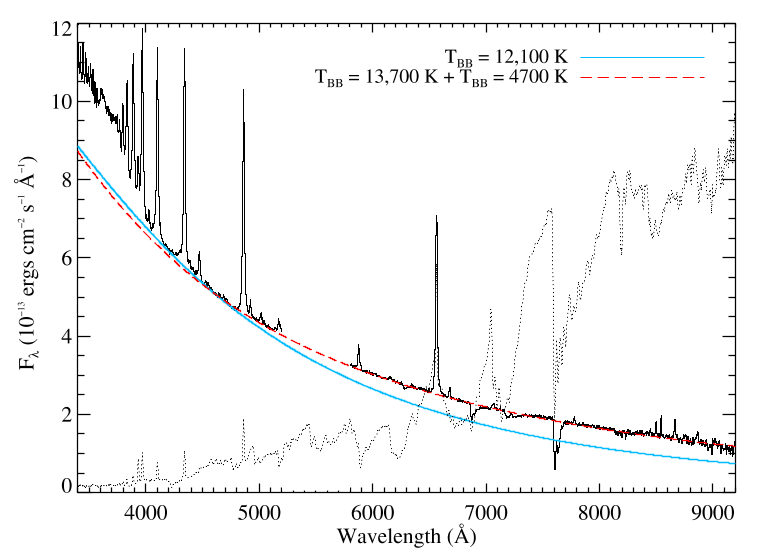
Figure 10: Flare spectrum at the peak of the large, impulsive-type (IF) event on YZ CMi in Fig. 9. Several blackbody fits to optical ($\lambda\geq 4000$ Å) continuum regions are shown. The flare spectrum (black) has the pre-flare (dotted) spectrum subtracted. Figure reproduced from [414] with permission.

The broadband photometry observations from Hawley and Pettersen [297] established the 9500 K blackbody hypothesis for the continuum in an energetic $E\sim 10^{34}$ erg flare from the M3Ve star AD Leo (see Sect. 8.2 for additional discussion), which was verified in [414] by fitting a blackbody temperature of $T\approx 11,600$ K to the optical range in the spectra of this flare. Further spectral investigation at resolving powers of $R\sim 500-1000$ in other events has revealed that a $T_{\rm{BB}}\approx 8500-14,000$ K blackbody color temperature in the blue-optical, $\lambda=4000-4800$ Å, is not a unique property of extremely energetic, large amplitude flares: for example, similar color temperatures were calculated in the impulsive phase flare spectrum (Appendix A) of the IF event in Fig. 8(bottom), which has an energy of $E_{U}\approx 1.6\times 10^{31}$ erg [416]. Hot blackbody-like continuum radiation in the blue-optical regime tends to be more prominent, or more often reported, in the rise and peak phases of impulsive-type (IF; Sect. 6.1) events. The flare event in Fig. 10 is a highly impulsive event. We refer the reader also to the discussions in Kowalski et al [416] and Kowalski [409] pertaining to the variation in the optical blackbody color temperatures on $\Delta t=3$ s cadences in the large, IF-type events listed in rows (1a) and (1b) in Table 7.

In echelle flare spectra with high-resolving power, Schmitt et al [661] and Fuhrmeister et al [241] have shown that the continuum radiation within the $U$ band at $\lambda=3250-3860$ Å  also exhibits hot blackbody color temperatures of $\approx 11,300$ K in the impulsive phase (Fig. 11a). At lower resolving power, similarly blue spectral trends at wavelengths shortward of the Balmer limit have been noted in Kowalski et al [414] for a large sample of flares. Though spectral observations within the $U$-band benefit from increased flare contrast, especially afforded by M dwarfs, accurate measurements are generally very difficult due to the systematic uncertainties of the flux calibration near the terrestrial atmospheric limit.

Spectral observations with high signal-to-noise (S/N) at $\lambda>3600$ Å reveal a very important clue about the origin of the white-light continuum radiation and its hot blackbody-like property. An extrapolation of a blackbody function that is fit to $\lambda=4000-4800$ Å (thus giving $T_{\rm{BB}}$), or an extrapolation of a blackbody that is fit to the continuum flux ratio, $f^{\prime}_{4170\rm{\AA}}/f^{\prime}_{6010\rm{\AA}}=$C4170${}^{\prime}/$C6010^′ (thus giving $T_{\rm{FcolorR}}$), fails to account for excess continuum flux at wavelengths shorter than $\lambda\lesssim 3700$ Å. In other words, there is a Balmer jump between the blue-optical continuum flux and continuum flux at shorter wavelengths within the $U$ band. An isothermal blackbody function thus does not comprehensively explain the panchromatic continuum flux properties. A Balmer jump was tentatively noted in Kunkel [428] and Moffett [506], and it was clearly evident and extensively characterized in impulsive-phase flare spectra using modern instrumentation and high-time resolution in Kowalski et al [414, 416]. An impulsive phase spectrum during a $E_{U}\approx 10^{31}$ erg, gradual/hybrid-type flare on GJ 1243 is shown in Fig. 11(b) over a broader spectral range than in panel (a). This is one of two flares analyzed in [420] that produced similar decreases in the continuum flux into the NUV range at $\lambda<3200$ Å, as constrained by Hubble Space Telescope data (not shown here). The Balmer jump in this event is the largest that has been detected spectroscopically over the impulsive phase of an M dwarf flare. In flares with very prominent hot blackbody-like continuum radiation at optical wavelengths, such as the Great Flare of AD Leo and the flare in Fig. 10, the Balmer jumps are evident as smaller flux excesses above the blackbody extrapolations to $\lambda\lesssim 3700$ Å.

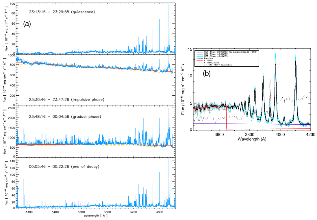
Figure 11: (a) VLT/UVES echelle ($R\sim 40,000$) spectral observations at $\lambda<3860$ Å that nearly extend to the terrestrial atmospheric cutoff. These spectra show the evolution of a giant white-light flare on the M6Ve star CN Leo, reproduced from [241] with permission. A $T\sim 11,300$ K blackbody is fit in the impulsive phase (2nd from top), and the gradual phase spectrum is fit with a $T\sim 9100$ K blackbody in the third panel. A catalog of the emission lines in the spectrum in the middle panel, extending to $\lambda=3060$ Å, is available through VizieR. (b) Other MVe flares in the impulsive phase show a large Balmer jump and a flatter $U$-band continuum spectrum that decreases into the NUV at shorter wavelengths than shown here [420] are not satisfactorily explained by a $T\approx 9000$ K blackbody fit to the blue-optical continuum wavelengths. Here, the two blue-colored spectra correspond to the rise/peak phase and early gradual decay phase, respectively, which are averaged into the black spectrum. The red-colored spectrum is an optically thin hydrogen recombination continuum model from a RHD simulation that invokes a solar-type electron beam heating function; the model is scaled to the observed spectrum at $\lambda\approx 3615$ Å. The spectra have a low-resolving power, $R\approx 600$, which is clearly sufficient for robust wavelength-integrated emission line fluxes. Figure reproduced with permission from Kowalski et al [420].

Impulsive-phase continuum flux ratios, which are “colors” if they are converted to magnitude differences, are calculated from flare spectra in [414], [416], and [420] and are shown in Fig. 12. Flux ratios have been calculated from isothermal static, slab models for $\tau(\lambda)\ggg 1$ (blackbody) and $\tau=0$ (continuous hydrogen LTE emissivity; Appendix C) and are shown in Fig. 12 for comparison. The flare peak “color-color” diagrams from the spectra demonstrate that the Balmer jump strengths ($f_{3615}^{\prime}$/$f_{4170}^{\prime}=$C3615${}^{\prime}/$C4170^′) imply that moderate-to-large continuum optical depths develop in stellar flare atmospheres. Further quantitative understanding about the observed offsets from the blackbody line in Fig. 12 requires detailed RHD model spectra, which are represented in the figure by the thick dashed line. These RHD model calculations include wavelength-dependent opacities and optical depths over column mass/depth-dependent temperatures and electron densities (Sect. 8.2), which are not included in blackbody or other simple slab models.

In Appendix B, we discuss comparable color-color diagrams using narrow-band ($\Delta\lambda=50-100$ Å) filters around $\lambda=3500$ Å, $4170$ Å, and $6010$ Å, which were designed specifically to avoid emission lines in flares and to measure the Balmer jump with the ULTRACAM instrument [169]. These narrow-band filters provide high-cadence ($\Delta t\approx 0.3-3$ s), simultaneous constraints of continuum variations while avoiding degeneracies in model fits to broadband filters (Sect. 7.2.4). ULTRACAM count-flux ratios from a large sample of MVe flares were analyzed and converted into flare-only continuum flux ratios in [416]. The flare color from relative photometry is the ratio of two values of

$$I_{f}(t)\langle f_{q,\lambda}\rangle_{T}$$ (12)

in the notation of Equation 7. Several flares were observed simultaneously with spectra over the impulsive to gradual decay phases, which facilitated unambiguous interpretation of the filter ratios (cf Figure 3 in Kowalski et al 416). A relationship between color temperatures fit to blue-optical spectra and to blue-to-red optical flux ratios is characterized by an offset of $\Delta T\approx 1900$ K (see Table 5 in Kowalski et al 416), in line with the various blackbody fits to the peak flare spectrum in Fig. 10.

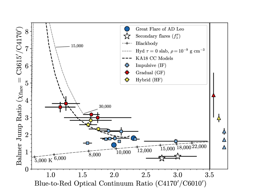
Figure 12: Compilation of impulsive-phase continuum flux ratios (color-color diagrams) from spectra [414, 416, 420]. The y-axis is a measure of the Balmer jump ratio, and the flux ratios on the x-axis correspond to optical color temperatures. Note that the $x$ and $y$ uncertainties are correlated, but only marginal error bars are shown. The prime symbols indicate that a pre-flare flux has been subtracted. The optical continuum colors from the Great Flare of AD Leo [297] are estimated from extrapolations of blackbody curve fits over the $\lambda=3800-4440$ Å range [414]. The wavelength range of C4170^′ can be seen in the right panel of Fig. 11. The flux ratio values at the peaks of flares indicate optical depths between blackbody radiation and optically thin hydrogen recombination radiation. The general trend is well-reproduced by approximations [KA18 CC models; 410] to the dynamic atmospheres in RHD simulations (Sect. 8.2). In the right margin plot, flares with Balmer jump measurements only are shown. The flares are color-coded to their $U$-band impulsiveness (IF/HF/GF) classification. Other flare-peak flux ratios from narrowband ULTRACAM photometry [416] are summarized in Appendix B. The color temperatures corresponding to the blue-to-red flux ratios in this figure are typically $\gtrsim 1500$ K less than that obtained from spectral fitting over the $\lambda=4000-4800$ Å range. All data in this figure are provided in supplementary online material hosted on Zenodo.

7.2.2 The Decay Phase and The Evolution of Optical Spectral Properties

The $T\approx 10,000$ K blackbody-like optical color temperatures do not last for long during MVe flares [e.g., 414, 409]. After the peak of a broadband (e.g., $U$-band) light curve, a gradual decay phase almost always follows a shorter period of faster decay. A characteristic blue-optical, blackbody color temperature value at the start of the gradual decay phase is $T_{\rm{BB}}\approx 8000$ K [414]. For equal $\lambda\approx 3615$ Å flare-only flux levels during the fast rise and fast decay phases, the fast decay phase is more than $\Delta T\approx 1000$ K cooler. [505] observed similar trends for optical color temperatures using continuum data during several MVe flares at $\lambda=4200-6900$ Å (e.g., see their Figure 3). At red-optical wavelengths, the continuum becomes very flat in the gradual decay phase, with even cooler temperatures. This was referred to as a red “conundruum” in [414]; the cooler blackbody fits were linked to the increasing fraction of energy that was previously reported in the redder bands of photometry in the decay phase of the Great Flare of AD Leo [see Figure 10 and accompanying discussion in 297] and retrospectively to the deviations from blackbody fits to the photometry of that flare (bottom right panel of Figure 11 in Hawley and Fisher 295). See Figure 31 of [414] for examples of the stellar flare gradual phase continuum spectra that exhibit cool $T\lesssim 5000$ K blackbody color temperatures in large dMe events. In smaller flares, it is difficult to accurately subtract the preflare spectrum at $\lambda\gtrsim 7500$ Å [420] and thus determine the NIR continuum properties.

It is not clear how to explain such persistent flat optical continua with relatively moderate-sized Balmer jump ratios; optically thin (bound-free) Paschen continua and photospheric backwarming predict cooler color temperatures but also much larger Balmer jumps, which are not observed – hence the conundrum. A related phenomenon during the impulsive phase may be the cause of the lower color temperatures that are calculated over a very wide optical wavelength range (such as those on the x-axis in Fig. 12) that spans the blue-optical and red-optical regimes. On the other hand, [241] report hotter blackbody temperatures over the red-wavelengths (not shown) in the flare in Fig. 11a. Clearly, further characterization of the red-optical and near-IR continuum properties is warranted. There may be important contributions to Kepler flare energetics in the gradual decay phase [304].

At shorter wavelengths within the $U$-band, the Balmer jump ratio increases in the gradual decay phase of a flare. The fraction of the wavelength-integrated energy in emission lines (primarily the hydrogen Balmer series in the optical and within the $U$-band wavelength range) also becomes larger. The energy partition evolution is shown in Fig. 13 for a large sample of dMe flares. It was found that the impulsive flare (IF) events were more continuum-dominated than the gradual flare (GF)-type events in both the impulsive phases and gradual phases of each event. Thus, an empirical connection among the broadband impulsiveness, fraction of energy in the Balmer component, Balmer jump strength (right panel of Fig. 13), and Balmer line-to-continuum ratios (namely, the H$\gamma$/C4170^′ ratios – see Appendix B) was established from simultaneous spectral and broadband photometry observations [see also 416, 420].

Stellar flares in the NUV generally exhibit a rapid time evolution [87]. However, the spectral properties in the NUV ($\lambda=2000-3200$ Å) are not nearly as well-observed as in the optical, in either impulsive- or gradual-type flares. The NUV spectral observations and model predictions are compiled and reviewed in [88]. [420] investigated the NUV properties in two HF-type events (that show some optical spectral properties that are more in line with other GF-type events) with shorter-wavelength spectra ($\lambda=2440-2840$ Å) from the Hubble Space Telescope / Cosmic Origins Spectrograph. They concluded that a Balmer continuum enhancement upon a blackbody-like optical continuum component is necessary to account for the continuum flux down to at least $\lambda\approx 2500$ Å. International Ultraviolet Explorer (IUE) FUV spectra covering $\lambda=1900-3100$ Å have been reported in the decaying phases of two large events on MVe stars [297, 630]. For a review of the timing of the IUE/NUV and IUE/FUV spectral integrations within the AD Leo Great Flare, see [408]. Of the few (relatively small) flares with NUV spectra that have been analyzed through their peak and decay phases, the fractions of energy in the continuum were calculated in the large range of $\approx 50-90$% [303, 420], which is much larger than in quiescence (35%). The evolution of the $\lambda\approx 3300-3800$ Å continuum-to-line energy fractionation is also noticeable after the peak phase in the M5.5/6Ve event in Fig. 11(a).

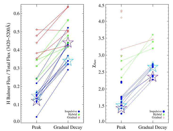
Figure 13: Energy of the hydrogen Balmer component vs. the optical continuum energy evolution in a large sample of MVe flares (reproduced from Kowalski et al 414 with permission). The Balmer jump ratios ($\chi_{\rm{flare}}$) increase into the gradual decay phase and are also generally correlated with the IF/HF/GF classification scheme. The hydrogen Balmer component includes an estimate for the Balmer continuum flux above an optical continuum model extrapolation to $\lambda<3650$ Å. Several more flares with comparable spectroscopy [416, 420] since this result have been consistent with these trends.

7.2.3 Empirically-determined, Broadband Radiated Energy Budgets Relative to the $U$ band

Empirical radiative energy fractionation from the X-ray to the radio provides model-independent characterization of stellar flares. The energy in the optical and NUV continuum provides a large contribution to the fractionation. To date, [562] is the most comprehensive analysis of the multi-wavelength energy budget in archival observations of stellar flares across a wide variety of spectral types and quiescent activity levels. At $\lambda=1200-8000$ Å, 96% of the peak flare luminosity can originate from the continuum in the impulsive phase [297]. In the gradual decay phase, the continuum accounts for as much as 83% when the emission lines remain highly elevated for longer durations (e.g., Fig. 9). The energy radiated in soft X-rays (0.04 - 2 keV) is estimated to be $\sim 11$x the H$\gamma$ energy [104] and to be comparable to that in the $U$-band, which is roughly 1/6 of the integrated $1200-8000$ Å white-light energy [297, 298], and a factor of 1/10 of the bolometric flare energy [562]. [297] constrain $E_{U}=0.64E_{2000-3260\mathrm{\AA}}$, however the bandpass-averaged energy [erg $\rm{\AA}^{-1}$] in the $U$-band is reported as a factor of 1.2 greater. Several estimates of the $U$-band to Kepler-band (Kp) energy ratios have been empirically determined to be $E_{U}=(0.4-0.65)E_{\rm{Kp}}$ [304]. [433] determine $E_{U}=1.2E_{B}=1.8E_{V}$. Line-integrated flare energies in H$\alpha$ are typically factors of $\gtrsim 0.04-0.08$ smaller than the $U$-band energies, and the H$\gamma$ energies are factors of $\approx 0.08$ of the $U$-band energies over several orders of magnitude in total flare energy [see the large compilation in Figure 4.2 in 406].

The relative energy in soft X-rays ($E\approx 0.1-5$ keV) is difficult to compare among flares. This difficulty arises due to different temporal [e.g., 298] and wavelength integration limits (e.g., by including a significant portion of the EUV range) among datasets. The X-ray and optical thermal radiation occur on much different time-scales (Sect. 7.7), and a limiting assumption [e.g. 38, 39] is sometimes that the broad-band flare energy is accurately accounted for with a scaled 2-temperature quiescent coronal model [281]. Nonetheless, many interesting empirical constraints on the X-ray to optical flare energies are reported in the literature. The ratio of the soft X-ray (and/or EUV) to the $U$-band energy can take on a large range of values, from essentially no detectable response in the soft X-rays within a $\pm 10-20$ minute window [177, 567]), down to $1/3$ [298], to as large as a factor of $\gtrsim 10$ [283, 571]. [527] study the X-ray properties (Sect. 11) of several X-ray flares with NICER spectra. The $E=0.5-10$ keV soft X-ray energies fall in the range of $0.3-1\times 10^{32}$ erg, but the event with complete multi-wavelength coverage in their study showed an H$\alpha$ response without a detectable $g^{\prime}$-band (white-light) response. In general, using the energy fractionation relation of $E_{U}=1/3E_{0.01-10\rm{keV}}=1/3E_{\rm{XEUV}}$ in [562], one obtains consistent cumulative flare rates in the XEUV and in the $U$-band [e.g., $\sim 1$ per day greater than $10^{32}$ erg in $U$ 590] corresponding to $1$ flare per day with $E_{\rm{XEUV}}\gtrsim 3\times 10^{32}$ erg [39] for non-simultaneous flares on AD Leo. [722] calculate the energy ratios of six simultaneous $U$-band and soft X-ray ($E=0.2-12$ keV) flares to be $E_{\rm{SXR}}/E_{U}\approx 1.5$. [662] extend the comprehensive, multi-wavelength analysis of a $E\approx 10^{34}$ erg flare on the K0Ve star AB Dor from [434]; they also report comparable energies released in soft X-rays and in an NUV bandpass. This is consistent with a paradigm that a majority [562, 431] of the total bolometric response in many (but not all) white-light stellar flares occurs from energy deposition in the dense, chromospheric footpoints (Fig. 2(right)).

The peak radio (3.6 cm) specific luminosity (erg s^-1 Hz^-1) is $\sim 1/4$ of the $U$-band, but the bandpass-integrated energy is a factor of $\mathcal{O}(10^{4})$ smaller [567]. New broadband observations have suggested much larger energy releases than expected in the NUV regime relative to the optical [88], while others are rather well-matched by current RHD models that invoke large heating rates [571, 420]. Studies of high-cadence, simultaneous Galex/FUV and Galex/NUV photometry have reported much larger peak luminosities in the broadband FUV than in the broadband NUV [632] (but see the discussion of bright Galex sources in Sect. 7.3). In the NIR, Davenport et al [156] present model predictions for the magnitude enhancements and energies relative to the $U$ band. [714] used high-cadence, high-precision monitoring of $\Delta U=-1.5$ mag flares on mid-type M dwarfs to constrain the broadband NIR response to $|\Delta_{\rm{NIR}}|\lesssim 5-12$ milli-magnitudes.

7.2.4 Optical Broadband Flare Colorimetry

Optical flare colorimetry is the study of the temporal tracks of broadband flare colors or absolute fluxes. For example, the $U-B$ vs. $B-V$ colors of flares on the dM3.5e star EV Lac were compared to regimes of optically thick and optically thin hydrogen spectra in [797]. They conclude that the flare continuum becomes optically thick (and more blackbody-like) in the peak phase of flares, but in the decay phase, the optical depths decrease. [302] find a best-fit blackbody temperature of $T\sim$8500 K by fitting to the fluxes in $UBVR$ filters for a sample of eight moderate-sized flares on AD Leo. Colorimetry with the traditional Johnson/Bessell bandpasses is a powerful and convenient method to test a wide variety of flare continuum models [428, 518, 522, 140, 179, 295, 468, 528, 88], and similar methods using broadband filters in the NUV and FUV have inferred a wide range of even hotter blackbody temperatures, $T\approx 20,000-50,000$ K [632, 259].

However, there are several important assumptions in broadband colorimetry that warrant spectroscopic verification or calibration [e.g., 416]. We discuss a few here. First, a correction to the contribution from emission lines in the optical bandpasses must be considered [297, 295]. The $V$ band is relatively free of major flare emission lines, but the contributions from the Balmer lines vary from flare to flare in the $B$ band (e.g., Fig. 13, Fig. 33 in Appendix A). The $U$ band integrates over the Balmer jump, a pseudo-continuum of blended Balmer lines, and to a lesser extent Ca II K and H emission. [9] demonstrated that a RHD model spectrum with a large Balmer jump and a discontinuity at $\lambda=3646$ Å exhibits colors that are consistent with a $T\sim 9000$ K blackbody when convolved with the $UBVR$ filters – but a blackbody function has no Balmer discontinuity or jump! [420] convolved an observed flare spectrum with broadband filters and showed that very large blackbody temperatures $\approx 15,000-22,000$ K could be inferred if the Balmer jump and high-order Balmer lines are not included in a model for the $U$-band and/or a constraint on the NUV continuum flux is not available (see their Figure 16). They showed that the full optical continuum regime may be flatter than a hot blackbody fit to the blue-optical wavelengths in such flares. The analysis of [302] included a bona-fide continuum flux constraint from HST spectra in the FUV, which may have otherwise resulted in much hotter peak blackbody temperatures, as in [797].

The results from broadband flare colorimetry have largely motivated spectroscopic investigations [261, 297, 414] of flares and detailed modeling [295], which will be discussed in Sect. 8.2.

7.3 FUV Observations: The Rapidly Evolving Flare Transition Region (TR)

The FUV continuum and emission line response may be a complex mixture of thermal, nonthermal, and nonlocal radiative processes in the flare transition region ($T\gtrsim 50,000$ K) and the deeper atmosphere at $T\lesssim 10,000$ K [297, 591, 302, 43, 237, 408, 182, 183]. Many questions remain about the origin of the spectral and temporal properties in stellar flares in this wavelength regime. A few observational properties are summarized in this section.

Hawley et al [302] presented a comprehensive, high-resolving power ($R=70,000$) study of eight moderate-sized M dwarf flares in the FUV with contemporaneous optical spectroscopy and broadband photometry. The energy budgets and timing properties in the brightest spectral lines and continua were compared in detail. In the biggest flare, the peak line fluxes in C II$\lambda$1335, Si IV$\lambda$1394, C IV$\lambda$1548, and C III$\lambda$1176 were calculated in the ratio of $\approx$ 25:35:50:100, respectively (note that the lineshifts in this study are discussed in Sect. 10). The study also presented a novel timing analysis of the light curves of Si IV, C IV, N V, and the FUV continuum region (averaged over $\lambda\approx 1266-1295,1420-1452,1675-1710$ Å) compared to the $U$-band by fitting $b$ and $m$ in the relation $\log_{10}$($F_{X}$) $=b+m$ $\log_{10}$($F_{U}$). For C IV 1551 and Si IV 1403, the slopes are rather consistent with a value of $\approx 1$, but the value of $m_{\rm{FUVcont}}\approx 1.7$ indicates a significantly more rapid evolution of the FUV continuum compared to the $U$-band, an effect that has also been noted in a much larger event on AD Leo [297]. The power-law relationship between the FUV continuum and the $U$ band is not yet explained by physical models. A linear scaling among neutral silicon FUV continua, C IV, and C II luminosities among a sample of dMe and RS CVn flares was interpreted in [591] to be consistent with radiative backheating of the temperature minimum region.

Remarkable M-star FUV flare spectra were analyzed in [297], [610], [465], [237], [471], and [216]. In nearly all cases, the continuum spectra are either very flat [in units of erg cm^-2 s^-1 Å^-1; see also the spectra compiled in 103, 90, 107, 591] or an isothermal blackbody continuum fit to the regions between emission lines results in $T\gtrsim 15,000$ K, up to $T\approx 30,000-40,000$ K. Of these, [297] and [471] had simultaneous multi-wavelength observations that were analyzed in detail, and [237] and [465] discuss redshifted line asymmetries in the FUV. [43] discuss interesting FUV continuum bursts during the gradual decay phase of a Si IV light curve in an energetic event from the young solar analog EK Dra (Fig. 14); similar responses during the FUV bursts do not show up in higher temperature lines. These continuum-only bursts were interpreted as possible stellar analogs of “Type II” white-light solar flares [210].

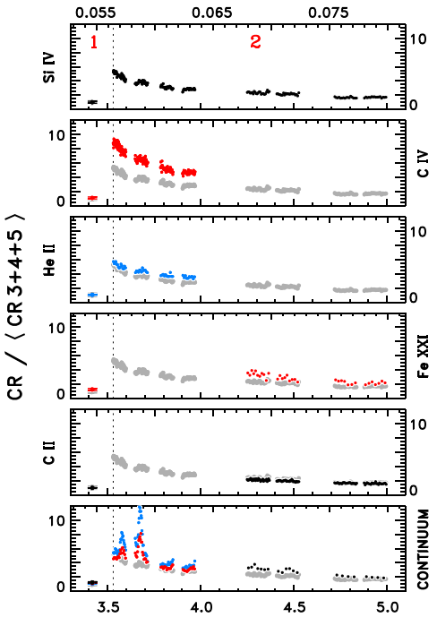
Figure 14: Figure 7 from [43], reproduced with permission, showing various FUV spectral quantities from HST/COS spectra during the decay phase of a large flare on the young solar analog, EK Dra. The bottom $x$-axis is elapsed time (hr) and top $x$-axis is rotational phase. Note the bursts that only occur in the FUV continuum ($\lambda=1435$ $\pm$ 25 Å, 1610 $\pm$ 25 Å). Later in the decay phase, shorter FUV wavelengths were observed by HST/COS, providing constraints on the continuum at $\lambda=1344.5\pm 6$ Å and $\lambda=1381.0\pm 8.0$ Å, the forbidden coronal line [Fe XXI]$\lambda$1354 ($T_{\rm{form}}\approx 10^{7}$ K), and C II$\lambda$1335.

Broadband comparisons of FUV and NUV responses during flares have been possible due to the time-tagged photon capability of the Galex mission. [632] analyzed a giant flare in both Galex bands, and [767] showed similar trends in other flares: very large ratios of the FUV to NUV fluxes that are far larger than expected from any known continuum model constrained by optical spectroscopy (Sect. 7.2). It has been pointed out that non-linearity corrections are important considerations at these large count rates in Galex [516, 228]. More recently, the gPhoton tool [502] has been employed to study events in the NUV without such concerns at large peak count rates, revealing remarkably fast time variations on a wide variety of stars [87]. Simultaneous constraints from Kepler and Galex observations favor very large flux ratios that are, again, far larger than RHD models of optically thick continuum radiation from high-energy electron-beam heating models [88].

Potential signatures of proton beams are found in both the FUV and in the gamma rays. [459] and [691] searched for gamma-ray stellar flares, which result from the higher energy ($E\gtrsim 30$ MeV / nucleon) ions and protons interacting with the stellar chromosphere. Lower-energy protons ($E\ll 1$ MeV) in the beams are expected to undergo charge-exchange with the neutral hydrogen in the chromosphere before it explodes in temperature. The nonthermal hydrogen beams then emit red-shifted Lyman $\alpha$ photons as a captured electron falls to the ground state. This is called the Orrall-Zirker effect [558, 388]. [777] reported a broad satellite component that was highly redshifted from Ly$\alpha$ and was attributed to low-energy proton beams in the early phase of a stellar flare in AU Mic. Follow-up observations with high-time resolution spectroscopy of the Ly $\alpha$ red and blue wings have not resulted in similar detections [629, 631, 216].

7.4 Centimeter (Microwave/Radio) Observations: Nonthermal Gyrosynchrotron Radiation from Mildly Relativistic Electrons

The radio/microwave regime at cm wavelengths (GHz frequencies) is a probe of nonthermal emission from accelerated electrons in flare coronae. Lower frequencies, $\lesssim 2$ GHz, tend to be highly circularly polarized, shorter in duration, and narrowband, indicating plasma or electron-cyclotron maser emission, while higher frequencies are largely unpolarized, broadband, and longer in duration. The unpolarized higher frequency radiation is consistent with gyrosynchrotron radiation from a power-law distribution of mildly relativistic electrons trapped in the magnetic fields of the flare region. The peak frequency of the gyrosynchrotron spectrum determines the demarcation at which the spectrum transitions from optically thin (at frequencies higher than the peak frequency) to optically thick (at frequencies lower than the peak frequency). For a homogeneously emitting source, the power-law index of accelerated electrons is directly related to the power-law index of the optically thin gyrosynchrotron flux spectrum at Earth; see [195] and Sect. 11 for more discussion and references.

Radio stellar flares have typically been observed in two bands, such as 6 cm (4.9 GHz) and 3.6 cm (8.4 GHz), which are close to or at lower frequencies than typical peak frequencies ($\approx 10$ GHz) [note that some solar flares have peak frequencies constrained to at least $\gtrsim 30$ GHz; 771]. A large multi-wavelength flare from the dM3.5e star EV Lac was studied in [567] and a light curve is shown Fig. 15. The peak radio luminosity at 8.4 GHz is $1.9\times 10^{15}$ erg s^-1 Hz^-1, but the $U$-band (not reproduced here; $L_{U,\rm{peak}}\approx 10^{30}$ erg s^-1, $E_{U}\approx 5\times 10^{31}$ erg) peaks about 54 s earlier and decays much more rapidly. The spectral index ($\alpha;S_{\nu}\propto\nu^{\alpha}$) evolution is discussed in [567] and indicates rapidly varying optical depths at these frequencies over the flare; in the decay phase, the higher frequency likely becomes optically thin, while in the peak phase, a reasonable range of expected power-law indices for the nonthermal electrons cannot explain the values of $\alpha$ for a homogeneous optically thick source. The lengthening decay timescales were interpreted in terms of the “trap+precipitation” model (Section 3). Source parameters were derived during the long decay, indicating very large loops on comparable scales to the stellar radius with small trapped nonthermal electron densities ($10^{4}-10^{6}$ cm^-3), and large magnetic fields (100 G) increasing over time and decreasing in source size as the higher frequency becomes more optically thin (R. Osten, priv. communication 2011).

Fig. 16 shows three radio flares from the comprehensive multi-wavelength study of the RS CVn system HR 1099 [566]. The data show low polarization during the flares and a similar spectral index evolution patterns among these long-duration flares. [280] and [687] present radio analyses of stellar flares that will be discussed below (Sect. 7.7, Sect. 11) in multi-wavelength contexts.

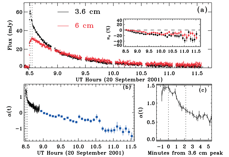
Figure 15: A remarkable radio flare on the dM3.5e EV Lac from [567] with the spectral indices calculated from observations at the two observed frequencies. Reproduced with permission.

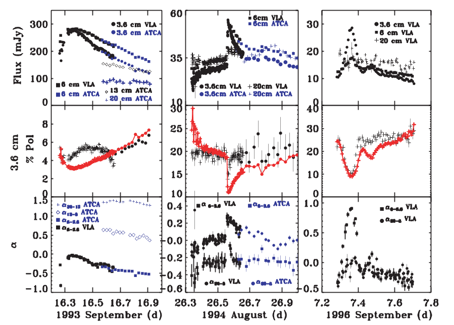
Figure 16: Flux (top row), polarization (middle row), and spectral indices (bottom row) during three gyrosynchrotron radio flares from the RS CVn HR 1099, reproduced from [566] with permission.

The emission at lower frequencies results from a plethora of possible phenomena. Decimetric flares can be very luminous and highly circularly polarized indicating coherent emission from beam-plasma instabilities (“plasma emission”) or electron cyclotron maser [437, 56, 560, 750, see references and discussion in Bastian 55, Güdel et al 280, Osten et al 567]. Coherent bursts can occur at higher frequencies too, and a remarkable example is the 100% left-hand circularly polarized 30 mJy peak-flux, 3-minute burst at 5 GHz discussed in [687] from the dM3e AD Leo. Assuming plasma emission, they derive a coronal electron density of $\approx 3\times 10^{11}$ cm^-3; assuming electron cyclotron, they derive a magnetic field of $B\approx 1.8$ kG. Between 1–2 GHz, stellar analogies to Type III decimetric bursts have been reported in very high time-resolution data from Arecibo [559]. A surprising lack of Type II radio bursts has been constrained in the context of extensive ground-based monitoring of optical flaring [144]. Many recent numerical, theoretical, and observational efforts have sought to explain the lack of Type II radio bursts from other stars [14, 521, 15, 776, see also Cliver et al 135].

7.5 Millimeter Observations from ALMA: Nonthermal Radiation with Linear Polarization

Bright nonthermal flare radiation occurs at much higher frequencies around $\nu\approx 230$ GHz ($\lambda\approx 1.3$ mm) too. Millimeter flares have been reported in ALMA data from AU Mic and Proxima Centauri [470, 469]. Particularly remarkable is the extremely impulsive flare from Proxima Centauri with multi-wavelength observations [471]. The dMe mm flares are short in duration ($2-30$ s), have rather symmetric (Gaussian-like) impulsive-phase time profiles, and exhibit only a very weak gradually decaying tail. They note that these properties are rather similar to the FUV continuum response in the same flares (see Sect. 7.3). The spectral indices, $\alpha$ ($S_{\nu}\propto\nu^{\alpha}$), are negative with a significant amount of linear polarization that “flip-flops” between negative and positive values during the peak phase.

The millimeter flare emission is interpreted as either an optically thin extension to the gyrosynchrotron radiation component that peaks around $\nu=10$ GHz (see the previous section), or as optically thin synchrotron radiation that undergoes some type of depolarization to the observed levels of $\pm 20$% [see 469]. The radiation sources are relativistic or ultra-relativistic electrons, but the magnetic field strengths are largely different between these hypotheses. Being in the optically thin regime of either interpretation, these observations have facilitated important inferences of the power-law indices of the accelerated electrons in the range of $\delta_{r}\approx 2.8-5.2$, indicating rather hard distributions of accelerated particles. At much higher frequencies, [66] reported short (FWHM durations of $\lesssim 1$ s) synchrotron bursts in the optical $U$-band superimposed on a giant, unpolarized dMe event from UV Ceti. Only lower limits on the linear polarization were possible, but the analyses of the energetics of the bursts favored very hard, $\delta<3.4$, power-laws of ultra-relativistic electrons.

Flares at $\nu\approx 100$ GHz ($\lambda\approx 3$ mm) have been reported from PMS stars, RS CVn’s, and eccentric binaries with colliding magnetospheres [592, 82, 647, 648, 100, 4]. In the case of the remarkable periastron event in the binary T Tauri V773 A [480], the flare was interpreted as synchrotron radiation. There is a notable observation of an RS CVn event at $\nu\leq 100$ GHz showing a break and a rise toward higher frequencies [57]: i.e., an opposite spectral index to the dMe events reported in ALMA, and one that is more similar to some reports in solar flares [383]. Colliding magnetospheres at periastron are also attributed to some flare-like optical and NUV variability in the PMS DQ Tau system [648, 259], while the optical variability properties at periastron at other times follow the expectations of accretion alone [482, 715].

7.6 Soft X-rays and EUV Observations: Loops Filled with Evaporated, Previously-Chromospheric/TR, $T>10^{7}$ K Thermal Plasma

Stellar flares have been studied in detail in soft X-rays ($E\approx 0.1-10$ keV) for many decades through XMM-Newton, Chandra, Swift, and NICER spectroscopy and photometry. X-ray flare spectra are a composite of many optically thin, highly-ionized emission lines and free-free bremsstrahlung continua that originate from the flaring coronal volume. The bulk of the radiation is thought to originate in the chromospheric gas that has been heated to millions of K and ablated into the magnetic loops, which confine the flows (Sect. 3). One of the highest signal-to-noise flare spectra during a stellar flare, which occurred in an RS CVn system, is showcased in Fig. 17.

An extensive review of stellar X-ray flares and analysis methods (prior to and including 2004) are provided by [276] and [277]. A general review of X-ray spectroscopy of stars is contained in [279]. Since 2004, there have been many important X-ray flare studies [567, 633, 697, 240, 545, 546, 573, 346, 448, 243, 574, 434, 599, 527, 578, 375]. In this section, we focus on a few key results from the last several decades pertaining to abundance changes and the stellar flare Neupert effect. Several other results are included throughout this review in other contexts where they are especially complementary (e.g., multi-wavelength analyses).

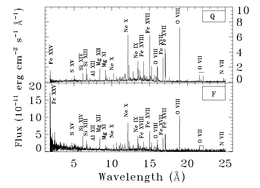
Figure 17: X-ray spectra from Chandra during quiescence (top) and flaring (bottom) in the active binary $\sigma^{2}$ Coronae Borealis, reproduced from [565] with permission. The authors note the enhanced continuum flux increasing towards shorter wavelengths in the flare spectrum.

7.7 The Neupert Effect in Stellar Flares

The backbone of the solar-stellar flare connection is the Neupert effect [540]. This was originally established in three solar flares as a correlation between the cumulative time-integral of the nonthermal microwave emission around 2.7 GHz and the thermal soft X-ray flux at 1.87 Å, attributed to the Fe XXV line emission (1s²–1s2p, which is sensitive to $T\approx 30$ MK). It has since been the subject of many follow-up studies in solar flares using either the hard X-rays or the derivative of the GOES 1–8 Å soft X-rays as a proxy for the nonthermal particle heating in the chromosphere [e.g., 165, 495, 739, 740, 761]. Alternatively, the empirical Neupert effect is expressed as a relationship between integral of the hard X-ray flux and the luminosity of the GOES soft X-rays. The relationship between the impulsive, early nonthermal radiation and the gradual, later-peaking thermal flux is thought to be linked by the physics of impulsive nonthermal particle propagation and bombardment of the chromosphere, rapid evaporation/ablation of $T\approx 10-50$ MK chromospheric mass into the coronal loops, and the eventual cooling to pre-flare coronal temperatures (Sect. 3).

The Neupert effect is also reported in multi-wavelength observations of stellar flares. Because stellar flare hard X-ray ($E\gg 10$ keV) emission is almost always too faint to detect, and radio observations are relatively difficult to plan and secure, the (thermal) response in the $U$-band is utilized as a proxy. This approach is justified by the close temporal and spatial correspondence between hard X-ray and white-light emission on the Sun [e.g., 370, 534, 345, 535, 231, 425, 426, 392]. A remarkable example of the stellar Neupert effect is shown for a flare from Proxima Centauri [283] in Fig. 18.

A stellar flare Neupert effect was first reported in [298] using the correlation between the extreme-ultraviolet (65–190 Å) flux and the integrated $U$-band energy during a long-duration, 3.5-hour rise phase of a flare from the dM3e AD Leo. This was followed shortly thereafter in [280] using a correlation between the $E=0.5-2$ keV soft X-rays and 3.6 cm radio emission during a flare on the dM5.5e UV Ceti A. The Neupert effect has subsequently been reported in stellar flares from RS CVn systems [284, 566], dMe stars [283, 285, 503, 758, 243, 108, 722], dK-stars [434], T Tauri stars [40]. There are also notable exceptions to the expected multi-wavelength relations from the Neupert effect in stellar flares [177, 567]; see these papers for discussions of possible explanations, which include deep heating from ultra-relativistic electrons or MeV protons. On the Sun, a clear violation of the Neupert effect in a “late impulsive [hard X-ray] burst” [adopting the terminology from 786] has been modeled with a large, low-energy cutoff $E\gtrsim 100$ keV in the nonthermal electron beam [761], which would reasonably generate small amounts of collisional heating within and chromospheric evaporation into the corona [however, the explanation is still being investigated; 6].

The Neupert effect in Flare D in [280] was investigated in detail and was compared to a similar multi-wavelength relationship in a solar flare from [165]. Intriguingly, the microwave response of flare D returned to pre-flare levels well before the maximum of the soft X-ray light curve, which is not in strict agreement with the expected Neupert effect. It was shown that similar deviations in the solar flare could be explained by a temperature sensitivity on the Neupert effect, such that radiation from hotter plasma more strongly followed the expectations [see also 495]. [280] thus separately derived a generalized Neupert effect for the light curve and a generalized Neupert effect, following energy conservation over the flaring coronal volume, $V$:

$$\frac{d}{dt}\Big{(}3n_{e}k_{B}TV\Big{)}=\alpha f_{\rm{radio}}(t)-n_{e}^{2}V\psi(T)$$ (13)

where $n_{e}$ is the ambient/thermal electron density of the heated plasma at a temperature $T$, $k_{B}$ is Boltzmann’s constant, $f_{\rm{radio}}$ is the flare radio flux as a function of time $t$, $\alpha$ is a proportionality constant, and $\psi(T)$ is the optically thin radiative loss function in units of erg cm³ s^-1. The left hand side of Equation 13 is the change of the thermal energy of the corona due to chromospheric mass evaporation, and the right hand side is the balance between radio/ microwave flux at Earth (assumed to be proportional to the kinetic energy of nonthermal electrons causing the chromospheric evaporation) and the optically thin radiative cooling of the coronal volume [assuming conductive cooling is overall small; see also 221]. Thus, accounting for the total plasma energetics and the bolometric luminosity evolution more naturally explains the apparent deviations from the Neupert effect assessed in a specific X-ray bandpass. An additional finding from the solar-stellar flare comparison was that the M dwarf flare was “radio-overluminous”, possibly suggesting a greater efficiency of acceleration of microwave-emitting ($E\gtrsim 100$ keV) electrons (Sect. 7.4) and/or a lower efficiency of chromospheric evaporation, among several other possibilities [see 280].

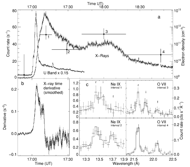
Figure 18: A remarkable example of the Neupert effect in a stellar flare in Proxima Centauri; figure reproduced with permission, from [283]. The $U$-band light curve is a (thermal) proxy for the nonthermal, impulsive energy deposition into the lower atmosphere. This flare was subsequently studied and modeled in [285] and [608].

The long rise times of Ca II K and H in dMe flares are suggestive of a Neupert-like effect, which could provide insight into their origin [e.g., through XEUV radiative backwarming; 295]. [414] investigated the relationship between the time-integral of the blue continuum flux around $\lambda=4170$ Å and the Ca II K line flux for a large sample of dMe flares. They found a Neupert-like relationship for a wide variety of flare types, both impulsive and gradual-type events, but none of these observations were complemented with X-ray data.

7.8 Abundance Changes

Impulsive heating in the chromosphere evaporates gas into the coronal loops, but all chemical elements are not evaporated equally. This results in relative abundance changes in the hot, coronal flare plasma such that elements with low first ionization potential (FIP) of $<10$ eV, like Fe, Si, and Mg, become preferentially enhanced above their photospheric values. The fractionation may be explained by ponderomotive forces [435] that selectively act on singly-ionized species in the upper pre-flare chromosphere.

Optically thin, coronal equilibrium modeling of X-ray and EUV spectra has been used to search for the so-called FIP effect (or its inverse, the IFIP effect) in stellar flares. Detections of changes in low-FIP abundances have been suggestive but not highly statistically significant [282], as have relative changes in high-FIP abundances such as Ne [567]. An example of an abundance analysis of an RS CVn flare in Fig. 17 is shown in Fig. 19 where an abundance change in Fe was seen, but other expected FIP dependencies were not. Recently, [578] searched for the (I)FIP effect in individual flares from the dM3.5e star EV Lac; they discuss the importance of field geometry in the context of the Laming theory. A homogeneous Sun-as-a-star (i.e., stellar) EUV spectral analysis of a large sample of solar flare Fe lines revealed coronal abundances that were remarkably close to photospheric, thus suggesting that chromospheric heating and evaporation occur deeper in the atmosphere than the standard models of electron beam heating and elemental fractionation [763], but [436] briefly contests the interpretation. Nonetheless, these solar results provide tantalizing connections to the deep heating rates (Sect. 8.2) that are inferred and hydrogen line blueshifts (Sect. 10) that are reported from optical observations of M dwarf flares.

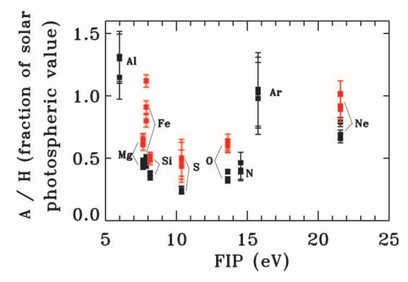
Figure 19: Abundances relative to hydrogen vs. the first ionization potential (FIP) in quiescent (black) and flaring (red) intervals in Chandra spectra of the RS CVn $\sigma^{2}$ Coronae Borealis. Figure reproduced from [565] with permission. They note that there is a slight enhancement of Mg, Si, O, and Ne during the flare, and Fe increases by nearly twice.

8 Atmosphere Modeling of Stellar Flares: Overview of Results

The physics of stellar flares is a complicated (and therefore interesting!) intersection of particle and nuclear physics, radiative transfer, plasma processes, gas dynamics and shock phenomena. All of the physical processes are inter-dependent and occur in a highly magnetized, coupled atmosphere, which is probably also highly turbulent. Flares are transient non-equilibrium departures of the stellar luminosity, and all layers of the atmosphere are thought to produce a response to some degree. In this section, we review different stellar flare modeling techniques. We focus on efforts toward understanding chromospheric flare processes in the context of the response of the entire stellar atmosphere. In contrast to purely magneto-hydrodynamic models, radiative models include detailed, time-dependent spectral predictions, which are critical for connecting to observations.

Stellar flare modeling can be sub-divided into several types of techniques. Isothermal, static slab modeling and atmospheric modeling are the two most general categories. Atmospheric modeling can be further divided into a static semi-empirical approach [e.g., 140, wherein the atmospheric structure is adjusted by hand to match observations] and radiative-hydrodynamic (RHD) forward modeling, whereby the input heating function is data-constrained and is not fine-tuned by the modeler to match observations [e.g., 9]. A hybrid, semi-empirical RHD approach is also possible, whereby the injected flare heating function is varied by hand over a large parameter space to find a time-dependent spectral response that matches the observations; thus, the atmospheric response and depth-dependent heating rates are calculated in a fully self-consistent manner [e.g., 415]. Though atmospheric modeling accounts for the vertical heterogeneity at a location in a flare source, additional techniques are required to model the lateral heterogeneity of the flare source and the source geometries (to be discussed further in Sect. 12).

8.1 Slab Models

Uniform, static slab modeling techniques include the following: fitting a Planck function to spectra or multi-band photometry [298, 302, 797, 414], calculating LTE continuum spectra for a range of optical depths $\tau(\lambda)=[0,\infty)$ [428, 197], and modeling the NLTE Balmer line decrements, optical depths, and continuum flux ratios [193, 364, 251, 512]. The pioneering study of Kunkel [428] found evidence for a prominent Balmer jump in their spectral observations of M dwarf flares. Their models of optically thin hydrogen (emissivity) continuum calculations, however, were largely inconsistent with the colors of M dwarf flares. They concluded that an additional moderately heated photospheric flare component could better account for observations (it was not until the radiative-hydrodynamic models of Allred et al [9] that essentially produced this scenario through a chromospheric hydrogen recombination spectrum and a radiatively backheated photospheric spectrum; see below). In Appendix C, we update the LTE hydrogen continuum emissivity calculations from Kunkel [428] with non-ideal occupational probabilities around the Balmer limit and extend them to higher temperatures and shorter wavelengths. These are useful for verifying for oneself how poorly first-principle simplifications hold up against continuum observations of actual stellar flares.

The higher quality spectral observations of the Great Flare of AD Leo [297] were found to (apparently) exhibit little to no Balmer jump in the flux, but there was unprecedented power in the optical continuum radiation and highly broadened hydrogen line wings. The broadband colors from the FUV through the optical ($R$ band) were tested against all of the models available at the time [295], and a $T\approx 8500-9500$ K blackbody was clearly favored over a hydrogen recombination model and a hot $T=10^{7}$ K free-free slab model interpretation; the former model has a slope that is too red, and the latter interpretation is inconsistent with X-ray to optical energy fractionations [see Section 4.3.2 of Hawley and Fisher 295, 562, and Sect. 7.2.3 here] and representative volume emission measures (Sect. 11). The various interpretations (blackbody vs.  optically thin Balmer continuum) and reported characteristics of the properties at the Balmer limit eventually motivated additional spectral observations [414]. More immediately, they paved the way toward advances in the realism of models of stellar flares. It became essential to consider the comprehensive atmospheric response that includes the complexities of depth-dependent heterogeneities of opacities, temperatures, and densities. Then, self-consistent non-equilibrium calculations of velocity fields, mass advection, radiative cooling, and flare heating became possible. We summarize these efforts next.

8.2 Atmospheric Models

A traditional approach to modeling stellar flare spectra is to start with a hydrostatic equilibrium model atmosphere and semi-empirically adjust the temperature gradients of the chromosphere, photosphere, and the location of a transition region. [140] explored the results of this technique using six atmospheric variations, including two very extreme adjustments where the chromosphere and transition region are placed at large column mass depths. They successfully reproduced a $T\approx 14,000$ K blackbody-like continuum spectral property in one of these models (their model #5), which also had very broad hydrogen lines and deep central reversals. Similar approaches have been widely adopted to model EUV, optical, and infrared stellar flare spectra [326, 489, 365, 131, 242, 654]. An example of this modeling technique from [242] is shown in Fig. 20, where the chromospheric temperature adjustments result in satisfactory fits to the emission lines in the giant CN Leo flare (Fig. 11(a)) from [241]. Further, a depth-dependent filling factor and missing photospheric heating were inferred through this technique.

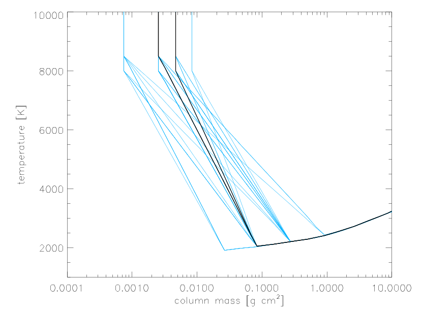
Figure 20: Demonstration of semi-empirical temperature adjustments used to model the red- and blue-wavelength optical spectra of a giant flare from CN Leo. Figure from [242] reproduced with permission from the author. See also [243] and [239] for similar approaches for modeling flares from Proxima Centauri and the dM6 star AZ Cnc, respectively.

How to create these deep transition region locations and chromospheres self-consistently with a flare heating function, $Q_{\rm{flare}}$? One early hypothesis [522] was that intense irradiation of soft, thermal X-rays from the flare corona penetrated to the low atmosphere, causing the optical emission lines and continuum in the gradual decay phase (whereas, the impulsive phase optical emission was assumed to be caused by particle beams, as was known to be consistent with hard X-ray and white-light timing in solar flares). [295] made a major advancement in stellar flare X-ray backheating models by calculating the full atmosphere, including the coronal structure. The apex temperatures were set and all else were determined self-consistently through energy balance (X-ray heating and photoionization v. radiative cooling) and hydrostatic equilibrium. Although the models produced hydrogen lines that were too narrow, and the optical and NUV continuum radiation was too weak compared to the observations [297], a large amount of broad, Ca II K line flux was predicted (perhaps offering clues to understanding its very slow temporal response). Updates to XEUV irradiation modeling (e.g., the atomic physics and geometrical assumptions therein) were employed in evolving atmospheres [296, 1, 8, 9, 10] that facilitated comparisons to the role of nonthermal electron heating. The role of reprocessing much larger X-ray emissivities into lower atmosphere optical continuum radiation in superflares has been recently reconsidered in static atmosphere calculations [543].

Significant advances were made in modeling the temporal evolution of the atmospheric response in gas-dynamic simulations, starting in the 1980s [458, 491, 224, 223, 222, 203]. An accurate treatment of energy deposition in a partially ionized, nonuniform chromosphere due to an injected nonthermal electron distribution was developed [296] based on analytic formulae for Coulomb collisions [199, 200]. With the inclusion of radiative-transfer, this effort resulted in a series of papers on radiative-hydrodynamic modeling of solar flares [2, 8] using a version of the RADYN code [113, 114, 115] that was configured for a larger surface gravity, a cooler photosphere, and a hotter and denser corona of an M dwarf in Allred et al [9]. The RHD simulations are currently limited to one spatial dimension, which facilitates resolving short-timescale shock phenomena, non-equilibrium ionization rates of hydrogen and helium, and detailed radiative transport.

The Allred et al. stellar flare models studied the atmospheric response to electron beam heating inputs from the first widely studied solar flare (SOL2002-07-23T00:30 GOES class X4.8) of the RHESSI [451] hard X-ray spectroscopic imaging era [167]. A double-power law distribution with a low-energy cutoff of $E_{c}=37$ keV was obtained from the hard X-ray modeling of [319], and several injected fluxes were investigated. These models reproduced the broad Balmer lines for the first time and bright optical and NUV continuum radiation. However, the Balmer jump was even more conspicuous than in the energy equilibrium models with X-ray flare irradiation [295] and semi-empirical models [242]. The dominant mode of radiative backheating in the RHD models takes place through irradiation of the photosphere by the Paschen and Balmer continuum fluxes of optically thin thermal radiation in response to the nonthermal electron beam energy deposition in the mid-to-upper chromosphere (the beam electrons do not penetrate to the photosphere; see Sect. 9). The detailed RHD spectrum provided an alternative explanation to the $T\approx 9000$ K blackbody interpretation of broadband photometry reported in earlier observations [e.g., 302], and the general shape of the Balmer continuum in the $U$-band was later found to be a satisfactory model in the decay phase spectra of a megaflare from YZ CMi [412]. The lower flux model was run for several minutes in [9], and it well-reproduced several transition region flare lines from [302]. Thus, the Allred et al. models provided a comprehensive solar-flare modeling framework for interpreting many of the observed properties of M dwarf flares.

Yet, re-analyses of archival spectra and new flare spectra and narrowband ULTRACAM photometry still did not match the shape and relative strength of the optical continuum radiation predicted by the highest-beam flux model in the [9] simulations. Some important details of the line broadening and blending at the Balmer limit remained unexplained as well (Sect. 10.2.1). The M dwarf gas-dynamic models of Livshits et al [458] produced a chromospheric condensation using a large nonthermal electron flux in an initially isothermal atmosphere and suggested that a large optical depth in the continuum could be produced well above the photosphere [see also 381]. [249] investigated chromospheric condensations as a source of white-light in solar flares. Impulsive-phase chromospheric condensations have been thought to be important in generating emission line spectral features in solar flares, such as the red-wing asymmetries in H$\alpha$ [349, 421, 528] and in more optically thin lines such as Fe II in IRIS NUV spectra [418, 274]. However, stellar radiative-hydrodynamic models did not produce chromospheric condensations that were dense enough to explain the observed continuum radiation until recently when the effects of very large electron beam fluxes were explored in RADYN [415] and the RH code [726]. (A realistic M dwarf atmosphere has a dense chromosphere and very efficient radiative cooling that can make the onset of complete ionization and explosive hydrodynamics a rather energetic threshold to attain, especially for a beam with a moderately large low-energy cutoff of $E_{c}=37$ keV, as traditionally employed in the RADYN dMe flare models.) The large electron beam fluxes were actually motivated by scaling the radiative backwarming fluxes from the Allred et al [9] models, but when the large beam fluxes were simulated, the lower chromosphere become too optically thick for the NUV and optical continuum radiation to penetrate to the pre-flare photosphere. Instead, the $\tau(\lambda)$ surfaces shift to a dense chromospheric condensation and the beam-heated layers just below the condensation (Fig. 2(right)).

A snapshot of the lower flare atmosphere in a RADYN model from [415] is shown in Fig. 21. The electron beam flux that is injected at the model loop apex is very large, $10^{13}$ erg cm^-2 s^-1 (which is hereafter referred to as a beam flux of “F13”, whereas “F12” refers to an injected beam flux of $10^{12}$ erg cm^-2 s^-1, and so on). By the time shown ($t=2.2$ s), the chromospheric condensation has cooled and accrued mass into a narrow $\Delta z\approx 15$ km region with a maximum electron density of $n_{e}\approx 5\times 10^{15}$ cm^-3. This was an exciting development because the model produced a small Balmer jump ratio and an optical color temperature that was in line with the impulsive phase spectral observations of dMe flares. In these models, the emergent optical radiative flux spectrum is a result of thermal response to the nonthermal electron beam energy deposition. The hydrogen recombination rates are determined by the Maxwellian velocity distribution of recombining ambient electrons, which are rapidly equilibrated as the beam kinetic energy is transferred to them (Sect. 9). Non-thermal ionization rates of hydrogen by the beam electrons (and subsequent nonthermal recombination) [340, 626, 3, 211] are much less than the thermal rates in these atmospheres at all times except for the first small fraction of a second. Optical and NUV spectral calculations with dominant non-thermal ionization rates [795] do not seem to predict the observed blue continuum properties and Balmer jump strengths (e.g., Fig. 10).

The formation of the optical and NUV continuum radiation in a F13 electron beam model is illustrated in Fig. 21. The cumulative contribution functions are shown for $\lambda=3550$ Å, $4300$ Å, and $6690$ Å. The detailed analyses of emissivity sources and optical depths explain the emergent spectrum as Balmer and Paschen recombination radiation from optically thick layers [see also 416, 407, for further analyses of these models]. The $\lambda=3550$ Å and $6690$ Å radiative fluxes are very optically thick and escape from the top of the condensation; the blue ($\sim 4300$ Å) continuum flux is less optically thick and emerges from the condensation and deeper layers that have a lower electron density of $n_{e}\approx 10^{15}$ cm^-3 and a lower gas temperature. The excitation by the highest energy electrons in the beam, and to a lesser extent, Balmer continuum backwarming, heat these deep layers and lead to an emergent spectrum that departs significantly from an optically thin hydrogen recombination spectrum from a homogeneous slab. [410] reported self-similar patterns in chromospheric condensation models (using a basic HI pattern recognition algorithm) and parameterized the RHD atmospheres at especially interesting times in their evolution. The two main parameters are a reference column mass ($m_{\rm{ref}}$) and a reference temperature ($T_{\rm{ref}}$), which are indicated in the cartoon in Fig. 2(right). These parameterized models facilitate LTE estimates of the Balmer jump and optical continuum ratios over a large range of condensation column masses and chromospheric temperature gradients. A prediction from [410] is shown in Fig. 12 for $T_{\rm{ref}}=11,000$ K and a range of $m_{\rm{ref}}$. The chromospheric condensation models can account for the trend over most of the impulsive-phase, flare-only Balmer jump ratios and optical continuum flux ratios in spectral observations.

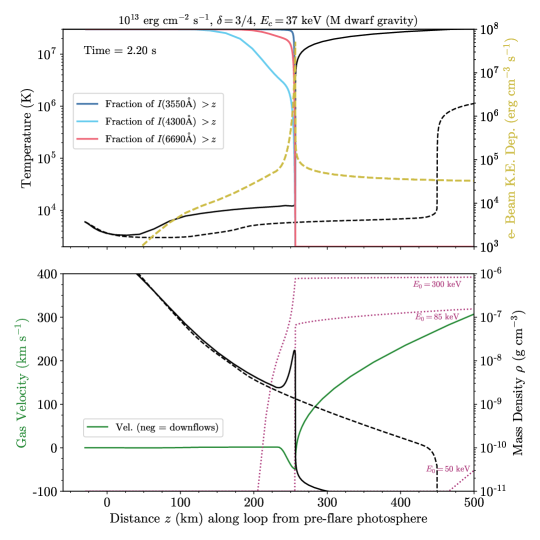
Figure 21: RADYN model of the low flare atmosphere after 2.2 s of heating by a high-flux, F13 ($10^{13}$ erg cm^-2 s^-1), double power-law electron beam [415]. (top panel) The cumulative of the contribution function to the emergent intensity, $I(\lambda=3550\rm{\AA})$, shows that the chromospheric condensation becomes optically thick in the Balmer continuum. The emergent blue-optical ($\lambda=4300$ Å) continuum intensity has larger contribution from the layers below the condensation, which is the large increase in gas density in the bottom panel. (Bottom panel) Several trajectories of nonthermal electrons are shown on top of the gas dynamic quantities (the initial kinetic energies are indicated, and the kinetic energy variations, $E(z)$, are normalized from 0 to 1 on a linear scale). The initial temperatures and gas densities are shown as black dashed lines. A movie is available online.

There has been follow-up work by Kowalski et al. on the modeling of chromospheric condensations to further evaluate their role as the origin of cooler line and continuum radiation in flares. Here, we summarize some of the challenges and successes with the hypothesis. First, these model atmospheres evolve very quickly, and the emergent flux spectra around the Balmer jump rapidly change on short timescales. Thus, an exposure-time averaged model spectrum does not necessarily exhibit properties that are consistent with the observational constraints. An average condensation model that produces a continuum spectrum that resembles observations requires a very hard, $\delta\approx 3$, electron beam distribution [e.g., 416, 418]. In other cases, an average model spectrum has satisfactorily produced the broadband continuum shape and Balmer jump strength in two moderate-sized dMe flares with HST/COS observations [420], and success has been achieved in an even broader-wavelength comparisons to a superflare event [571]. There are also important theoretical issues with the huge current density and charge displacement due to an electron beam with a flux of $10^{13}$ erg cm^-2 s^-1 that have not yet been addressed.

A further severe challenge has been encountered in dense chromospheric condensation modeling of dMe flares, as detailed in [418] and [408]. Updated hydrogen emission line broadening treatments (Sect. 10) reveal that the optical depths and the ambient (thermal) charge densities in the model condensations are far too large to be consistent with the symmetric broadening in archival dMe flare observations. [527] modeled the broad H$\alpha$ emission lines in a $E>10^{33}$ erg, $\Delta g\approx-1.35$ mag superflare from AD Leo. They used updated hydrogen broadening profiles in RADYN simulations and concluded that lower electron beam fluxes with hard power-law distributions produce optical depths and electron densities in the low atmosphere that explain the broadening. The models with energy transport through only thermal conduction were largely discrepant (Fig. 22).

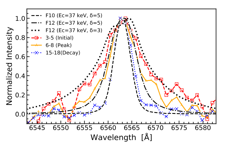
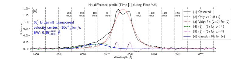
Figure 22: (Top) Model spectra of H$\alpha$ that were calculated with the RADYN code and analyzed in [527]. The larger electron beam heating rates reproduce the broad, symmetric Balmer lines in an AD Leo flare. Figure reproduced with permission from [527]. (Bottom) Echelle resolving power, flare-only spectra of the H$\alpha$ line during the decay of a large flare on YZ CMi. This figure demonstrates the phenomenological Voigt profile $+$ Gaussian modeling that is used to isolate and characterize the asymmetries in the wings of the Balmer lines. In this spectrum, a Gaussian model is fit to the broad blue asymmetry; reproduced from Fig. 42(a) in Notsu et al [552], with permission.

Similarly to [527], the approaches in [418], [408], and Brasseur et al [88] employ semi-empirical forward modeling with the RADYN and RH codes. These studies use large low-energy cutoffs ($E_{c}\geq 85$ keV), hard power-law indices ($\delta=3$), and high energy fluxes ($10^{12}-10^{13}$ erg cm^-2 s^-1) to heat the low chromosphere at $\log_{10}m_{c}/[\rm{g\ cm}^{-2}]\gtrsim-2$ to gas temperatures hotter than $10,000$ K [see also 409]. This approach results in optically thick continuum radiation at NUV and optical wavelengths and broad Balmer wings in the early impulsive and peak phase. However, an additional model component that is attributed to lateral spatial heterogeneity in the flare heating is required to simultaneously account for the narrow and broad components of the hydrogen Balmer emission line fluxes. The slow-rising Ca II K emission line flux is not yet explained with this approach. Large, low-energy electron beam cutoffs or some other energy transport mechanism [e.g., 401] that similarly results in a large fraction of the beam heating over $\log_{10}m_{c}=-2.2$ to $-1.2$ [409] rather than in the upper chromosphere ($\log_{10}m_{c}\lesssim-3$) seems to be a promising avenue for explaining some of the more challenging M dwarf flare observations. For example, a model with $2\times 10^{12}$ erg cm^-2 s^-1 and $E_{c}=500$ keV (i.e., a high-flux, fully relativistic electron beam) adequately reproduces the spectra of the secondary flare events in the decay phase of the YZ CMi megaflare [412, 414]. These events produced an “A star on an M star”, such that the flare-only spectra resembled the main sequence A0 V star, Vega. The Balmer lines and Balmer continuum are “in absorption”. The colors from two secondary events are shown in Fig. 12 as star symbols. Alternative explanations are summarized in [16]. [414] claimed that some flares show a narrowing of the hydrogen Balmer lines in their impulsive-phase peaks that is consistent with a spatially unresolved component on the star that has the hydrogen Balmer lines in absorption.

Relatively little attention has been given to the coronal and late phase predictions in the recent RADYN models of stellar flares. The RADYN models are generally viewed as simulations of the short, pulsed beam-heating events that sequentially light up along a two ribbon flare arcade, as in typical solar flare geometries (see Sect. 12). Ostensibly, the very hot $T\gtrsim 50$ MK coronal temperatures produced within a short time are expected to eventually cool down and shine in emission lines that probe cooler temperatures [295, 28]. However, it is imprudent to speculate further on these issues without X-ray spectral synthesis because of the vast range of electron densities over the hot temperatures in the model corona and transition region.

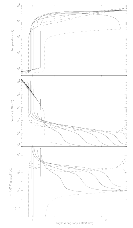
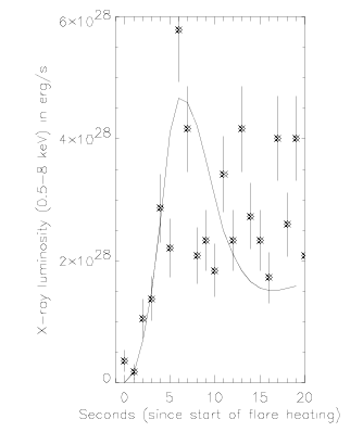
Figure 23: (Left) Hydrodynamic modeling of a coronal explosion on CN Leo. The panel shows temperature, number density, and the emission measure weighted cooling function. The solid lines show the evolution at $t=0,2,4,8,10$ s when a flare heating function was applied, while the dashed lines correspond to $t=13,16$, and $19$ s. (Right) Modeled X-ray light curve over the first 20 s of the model compared to XMM-Newton data of the early phase of the giant X-ray flare. Figures reproduced from [661] with permission.

[661] used the Palermo-Harvard adaptive regridding code [582, 69] to model the hydrodynamic response of the giant X-ray CN Leo flare in Fig. 11(a) over the first 20 s. They assumed a Gaussian heating function centered in the low corona and extended into the chromosphere. The atmospheric evolution is shown in Fig. 23. The flare transition region moves downward, and there is an increase in density that resembles a chromospheric condensation, but low-temperature spectral synthesis was not the goal of these modeling efforts [see 242, and Fig. 20 here]. They successfully reproduced the X-ray luminosity evolution by multiplying the model by an area of $10^{19}$ cm². The model X-ray luminosity is shown in the right panel of Fig. 23. They explain the early phase X-ray light curve as a result of heating within the bottom parts of a flaring loop during the first 10 s, followed by a $v\sim 1000$ km s^-1 evaporation upflow that dominates the coronal emission after that. Compressional heating at the apex occurs later on as well (see their dashed temperature profiles) and persists after the applied flare heating function is turned off at 10 s. The Palermo-Harvard code has modeled longer heating durations to simulate X-ray flares from the M dwarf Proxima Centauri [608] and the active giant HR 9024 as well [709, 20]. [608] model the second X-ray flare in the decay of the event in Fig. 18 here as the first in a series of loops. They develop a two-phase heating model whereby the total energy input consists of energy deposition near the loop apex and near the low-altitude coronal footpoints.

9 Atmosphere Modeling of Stellar Flares: Overview of Physics and Methods

9.1 An Introduction to Radiative-Hydrodynamic Flare Modeling

Radiative-hydrodynamic flare modeling consists of solving the coupled, non-linear conservation equations for mass, momentum, energy, charge, radiative transfer, level populations, and grid motion. The atmosphere begins in a steady-state, and flare heating is introduced through a term in the energy equation, $Q_{\rm{flare}}$. In this section, I follow the general framework and modeling assumptions employed in the RADYN flare code, which has unique capabilities for stellar flare applications (e.g., radiative transfer and non-solar gravity).

A conservation/continuity equation for a volumetric quantity $w$ ($w$hatever cm^-3), which is a function of space and time, can be written (in laboratory frame coordinates) as

$$\frac{\partial w}{\partial t}+\nabla\cdot(w\mathbf{v})=0$$ (14)

in three spatial dimensions (if the time-derivative is 0, then the equation leads to the steady-state solution), where $\mathbf{v}$ is the macroscopic gas velocity vector, $w\mathbf{v}$ is the flux of the quantity in $w$, and we have excluded a diffusion term, $-D\nabla w$ [765], in the parentheses. The second term is the advection term which is a gradient of the flux (while in more than one spatial dimension, it is the divergence of the flux). From here on, we discuss the 1D form of Eq. 14 and consider the spatial coordinate $z$ (“height”) along a hypothetical magnetic loop extending from below the photosphere to the loop apex in the corona. At the loop apex, the $z$ direction is parallel to the stellar surface, and the surface gravity in the momentum equation decreases accordingly. In 1D flare modeling, one assumes that flows and energy transfer are aligned with the magnetic field, meaning that the magnetic pressure is assumed to be much larger than the gas pressure everywhere at all times (which may be appropriate for the center of a strong magnetic flux tube). Note also that the typical 1D form of the continuity equation in Eq. 14 usually assumes a constant flux tube cross-sectional area; for a non-variable magnetic field along the flow direction, the adjustments that must be made to account for funneling effects are written in [203] and [612].

The conservation equations are solved simultaneously with an adaptive grid equation [175] using a semi-implicit numerical scheme that allows for timesteps that are much longer than the Courant step, which is very small in the transition region during flares. Implicit radiation-hydrodynamics essentially consists of linearization and iteration (i.e., multi-dimensional Newton-Raphson) of the conservation equations with a five-point stencil monotonic upstream scheme [735, 736] to ensure numerical stability of advected quantities around steep gradients, such as shocks. The spatial derivatives are written as finite differences and are centered in time between the current and next time (semi-implicitly) during the linearization of the Taylor-expansion about the iterative guesses. We do not discuss the details here and instead direct the interested reader to [394], [491], [112], [1] for general overviews. We especially recommend the lucid and comprehensive lecture on the topic in [174].

The Eulerian (fixed space) forms of the conservation equations that are solved in RADYN flare modeling are written in [10]. Here, I highlight the conservation of internal energy density, $e$, which is the first law of thermodynamics (i.e., $dU+PdV=Q$) connecting several of the critical ingredients in flare RHD:

$$\frac{\partial e}{\partial t}+\frac{\partial(ev_{z})}{\partial z}+(P+q)\frac{\partial v_{z}}{\partial z}=-\frac{\partial\left(F_{c}+F_{r}\right)}{\partial z}+Q_{\rm{flare}}+\sum_{n}Q_{n}$$ (15)

where $P$ is the thermal gas pressure from all species $s$ ($P=k_{B}T\sum_{s}n_{s}$) and enters into the $PdV$ work term, $v_{z}$ is the gas velocity along the loop axis ($z$ direction), $q$ is a viscous stress term added to aid in numerical stability, $F_{c}$ is the thermal conduction flux (temperature diffusion), $F_{r}$ is the radiative flux, and $Q_{n}$ can be any number of external heating terms, which can be flare-related (e.g., beam-generated electric fields) or non-radiative sources to keep the photosphere and corona hot in the pre-flare equilibrium state. The form of thermal conduction is taken from [685] and [224]. The internal energy density is the sum of thermal and excitation energy densities:

$$e=\frac{3}{2}k_{B}T\sum_{s}n_{s}+\sum_{s,i}n_{s,i}\chi_{s,i}$$ (16)

where $n_{s,i}$ is the population level density of species $s$ and level $i$ and $\chi$ represents atomic excitation energies ($\chi=0$ for the ground state). Equation 15 is derived by starting from the continuity equation (setting Eq. 14 equal to all $Q$ terms, instead of 0) for the energy density, $\varepsilon$, which is the usual [e.g., 712]:

$$\varepsilon=\rho\left(\frac{1}{2}v_{z}^{2}+e^{\prime}+\Phi\right)$$ (17)

where $e^{\prime}$ is the internal energy per unit mass ($e=\rho e^{\prime}$), $\Phi$ is the gravitational potential energy, $gz$. Magnetic energy density is neglected. The energy flux is

$$\mathfrak{F}=\rho\left(\frac{1}{2}v_{z}^{2}+h+\Phi\right)v_{z}$$ (18)

where $h$ is the enthalpy per unit mass (“specific” enthalpy; $h=e^{\prime}+\frac{P}{\rho}$). After substituting the continuity equations for mass density and linear momentum density, some algebra and reduction, the form of Equation 15 is readily obtained.

The equation of radiative transfer is solved simultaneously with the other equations through complete linearization and a low-order Feautrier method that is stable in the presence of steep gradients and shocks (M. Carlsson, priv. communication 2022). The monochromatic specific radiative intensity, $I_{\nu}(z,\nu,\mu)$, at frequency $\nu$, at an angle $\theta=\cos^{-1}\mu$ from the atmospheric normal, at a height $z$, is assumed to be in steady-state ($\frac{\partial I_{\nu}(z,\nu,\mu)/c}{\partial t}=0$ where $c$ is the speed of light; cf. Section 11.2 of Hubeny and Mihalas 337) within each hydrodynamic time-step. The solution to the intensity at each depth point is integrated over angle using a Gaussian quadrature numerical weighting [123], and then it is integrated over frequency to give the net radiative flux. The gradient in the energy equation (Eq. 15) thus gives the radiative heating or cooling rate at each time-step in the flare simulation. Due to this coupling, the time-history of the atomic level populations, ionization, rates, and radiative transfer are critical in the self-consistent energy balance, pressure gradients, and hydrodynamics in a flare simulation.

9.2 The Flare Heating Term

The flare heating term, $Q_{\rm{flare}}$, in the energy equation (Eq. 15) may be a sum from a large number of possible sources: nonthermal electrons, nonthermal protons, Joule heating, shocks in the reconnection process, and Alfven waves. Here, we assume the major source of heating in stellar flares is through nonthermal electrons, as is widely accepted in and borrowed from the solar flare analogy. The radio gyrosynchrotron radiation from mildly relativistic electrons in stellar flares also supports this approach (Sect. 11). The following is a synopsis of several relevant points from the collisional energy loss theory of [199] and a unified model calculation presented in [10]. Additional formalism about the theory of energy loss on ionized species and neutrals is contained in [723], [122], [200], [211], [296], [517], [688]. We consider particle velocities with magnitude, $v$, and three directional components (whereas in the previous section, one-dimensional bulk velocities of the ambient/thermalized gas were denoted as $v_{z}$).

A nonthermal (beam) electron penetrating a plasma deposits heat thus affecting the internal energy of the plasma by increasing the temperature, excitation, and ionization of the plasma constituents. A beam particle is assumed to begin with a kinetic energy that is much greater than the average kinetic energy of the free electrons in the background gas or plasma (thus, the background plasma is a “cold target”); the beam particle is then followed until it decreases to an energy that is close ($\sim 2.5k_{B}T$) to the energy of the thermal distribution, at which point it joins the background/thermal pool of particles. Energy loss from the beam electron occurs through Coulomb collisions, and the interactions with all particles in the plasma require an integral that, when evaluated (with somewhat artificially imposed distance limits), is known as a Coulomb logarithm [e.g., 61]. The Coulomb logarithms give a sense of the relative importance of distant to nearby interactions with the beam particle. A beam particle loses energy to ambient (thermal) electrons and protons, with an associated Coulomb logarithm $\Lambda$. The integral that describes collisions with ambient neutral atoms also has an associated Coulomb logarithm, $\Lambda^{\prime}$, for each neutral species. For a typical beam electron, values for $\Lambda$ and $\Lambda^{\prime}$ are $\approx 20$ and 8.5, respectively. Including the ionization fraction of a hydrogen gas, $x$, the fraction of energy loss that goes into the neutrals is [626] $\frac{1-x}{x\Lambda+(1-x)\Lambda^{\prime}}$. For a 50% ionized gas, the energy loss is about a factor of three more efficient on the ionized component (i.e., the ambient thermal electrons).

The pitch angle of the beam particle changes through scattering, which can be elastic (for collisions with ambient protons, electrons, and neutrals) or inelastic (for collisions with neutrals). The momentum changes in the direction parallel to the trajectory of the beam particle must include an additional Coulomb logarithm, $\Lambda^{\prime\prime}$, for elastic scattering off of neutrals (e.g., collisions with bound electrons that do not undergo atomic transitions). Distribution-averaged approximations to the Coulomb logarithms are given in [199] and [296]; [10, 11] gives the energy-dependent, relativistic formulae. Then, the total differential kinetic energy change per unit path length [keV km^-1] of an electron beam particle interacting with hydrogen and ambient electrons in a partially ionized gas is, following from Eq. 24a of [199],

$$\Big{(}\frac{dE}{dz}\Big{)}_{\rm{hyd}} =\Big{(}\frac{dE}{dz}\Big{)}_{\rm{hyd,I}}+\Big{(}\frac{dE}{dz}\Big{)}_{\rm{hyd,N}}$$ (19)

$$=-10^{5}\frac{2\pi e^{4}}{\mu E\times a^{2}}\Big{(}x\Lambda_{ee}+(1-x)\Lambda^{\prime}\Big{)}\gamma n_{\rm{hyd}}$$ (20)

which is the sum of the ionized (I) and neutral (N) components of energy loss in a hydrogen gas. We ignore the $\sim 10^{3}$ less energy loss on ambient protons, $E$ is the kinetic energy of the electron beam particle in keV, $a=1.602\times 10^{-9}$ keV erg^-1, $\mu$ specifies its pitch angle ($\mu=1$ for beamed along hypothetical magnetic field), $x$ is the ionization fraction of the hydrogen target, $n_{\rm{hyd}}$ is the number density of neutral hydrogen atoms plus ambient protons in the target, $\gamma$ is the relativistic gamma factor of the beam electron, and all of the rest of the units are in cgs. As an example, if $x=0.75$, $n_{\rm{hyd}}=1.7\times 10^{13}$ cm^-3, $T\approx 10^{4}$ K, which are representative conditions at the top of a model M dwarf chromosphere, then $\frac{dE}{dx}=-0.1$ keV km^-1 for $E=40$ keV. Additional energy losses on helium and other gas constituents can be included.

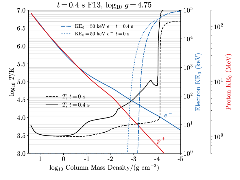
Figure 24: A pre-flare and flare model (from the RADYN code) of the temperature distribution in the low atmosphere compared to Coulomb stopping depths of beam particles. For reference the (pre-flare) photosphere and upper photosphere corresponds to $\log_{10}m_{c}>1$ on this plot ($m_{c}$ is the column mass density in units of g cm^-2). The collisional stopping depths of mono-energetic beam particles are shown on the right using Equation 19. The kinetic energy decrease of an electron with injected energy of 50 keV is shown for each state of the atmosphere; these two curves are on a linear scale and normalized to 1.0 at the top of the loop (where they are injected) outside the range of the plot on the right. An electron gets stopped at higher altitudes when the chromosphere has experienced a large amount of hydrogen ionization; as the atmosphere further evolves, the lower energy electrons in the beam can be stopped in the evaporation flows (cf. Fig. 21), and all the rest of the beam particles except for the highest energy electrons are stopped in the chromospheric condensation (Fig. 2(right)). Note, these “cold-target” stopping depth approximations for the protons are not accurate significantly below $\lesssim 1$ MeV at which the warm-target transport treatment becomes essential [11].

Assuming a fully ionized, uniform hydrogen plasma, Eq. 19 can be integrated from the electron’s initial energy $E=E_{0}$ to $E=0$ to find the stopping length of an electron, $L_{\rm{stop}}\propto E_{0}^{2}n_{e}^{-1}$, which defines an effective absorption cross section, $\sigma$, according to $\sigma n_{e}L_{\rm{stop}}=1$. Higher energy particles penetrate deeper because they have more energy to lose and because they spend less time losing energy per collision. The energy loss rate per electron is, $\frac{dE}{dz}\frac{dz}{dt}=dE/dt=-2\pi e^{4}n_{e}v\Lambda/E$ which can be integrated over a uniform plasma to give a timescale for energy loss, $\tau\propto E^{1.5}/n_{e}$ at non-relativistic energies. Note, this is the same proportionality in the estimate for scattering timescales out of a magnetic trap (Sect. 3).

The heating from a power-law distribution of electrons and protons is analytically solved in [199] following [97] and [450] in an integral from, $Q_{\rm{beam}}(m_{c})$, which is a function of column mass over an atmosphere with arbitrary, constant ionization fraction. [296] extended the formulae to atmospheres with non-uniform ionization fractions. The analytic formulae for $Q_{\rm{beam}}$ were used in RADYN simulations of stellar flares up through the models in [415, 416].

An alternative method is to numerically solve the distribution function, $f(z,\mu,E,t)$, of the nonthermal electrons [440, 494], and evaluate the spatial gradient/divergence. This is the Fokker-Planck solution [637], which tracks the phase space evolution due to systematic decrease (drag) and diffusion of the kinetic energies, $E$, and of the cosines of the beam pitch angles, $\mu$. Generally speaking, the Fokker-Planck solution is required when some or all of the following are important: time dependence of the beam propagation, diffusion of pitch angle and energy, external forces (e.g., magnetic mirror, synchrotron losses), and beam feedback effects such as return currents and plasma waves [293, 490, 794, 10]. We refer the reader to the comprehensive description of the collisional Boltzmann transport equation in [723] and the application of the Fokker-Planck solution to flare modeling in [11]. Other helpful references are [712] and [83]. In current RHD simulations, numerical limitations necessitate a steady-state solution ($\frac{\partial f}{\partial t}=0$) at each hydrodynamic time-step, thus giving the flare heating rate as:

$$Q_{\rm{flare}}(z)=Q_{\rm{beam}}(z)=\frac{d}{dz}\int_{\mu}\int_{E}\mu vEf(z,\mu,E)dEd\mu$$ (21)

which is the spatial gradient of the beam flux at height $z$ in the atmosphere.

10 Models of Chromospheric & Transition Region Flare Emission Line Broadening (& Asymmetries)

The emission line properties (strength and shapes) during flares encode much of the evolution of the atmospheric physics, which may be quite dissimilar to the density, optical depth, and velocity regimes in the atmosphere before a flare. The interpretation of flare emission lines, especially in the chromosphere, in general requires forward modeling with non-equilibrium physics. Thus, there is still much we do not know about the origin of certain well-observed changes in the spectral line profile shapes during flares. The efforts to make headway in this area have been stymied because, further, not all flares show similar behavior in the same emission line (cf. in solar flares, H$\alpha$ shows a rather wide range of empirical properties; Canfield et al 110). Detailed line shape measurements are further obfuscated by the heterogeneity of the flare source and long exposure times, which are generally required of echelle observations.

This section is divided into two parts. First, we categorize the line broadening mechanisms that are thought to be important in the interpretation of transition-region and chromospheric line widths and asymmetries during stellar flares (Sect. 10.1). Then, in Sect. 10.2, we summarize the symmetric pressure broadening of hydrogen lines in more detail. Observations and modeling are reviewed together in this section.

10.1 An Overview of Broadening Sources

There are many types of possible sources of chromospheric and transition region emission line broadening in stellar flare spectral observations. Microscopic broadening occurs over scales that are much smaller than the optical depth, and each process is generally assumed to be statistically independent. Thus, the total microscopic broadening enters the line opacity after a convolution of all the respective probability density functions. Microscopic broadening is largely a source of symmetric broadening (to first order). Macroscopic broadening sources can affect the line opacity though the mean intensity, $J_{\nu}$, but this term typically refers to the broadening from spatially unresolved, inhomogeneous sources in the plane transverse to the observer.

Here, we summarize the most important sources of micro- and macroscopic broadening that are relevant to stellar flare chromospheric, transition region, and photospheric lines. We exclude rotational and Zeeman broadening, which affect the broadening of lines in active stars in their quiescent states. Note that microscopic broadening sources are modeled with an ambient, thermal distribution of perturbers even when they are considered separately from thermal Doppler broadening. In Fig. 25 we show several profiles for the hydrogen Balmer $\gamma$ and $\alpha$ lines, which complement the descriptions throughout this section. For each type of broadening, we state the probability distribution that most closely describes the perturbation magnitudes.

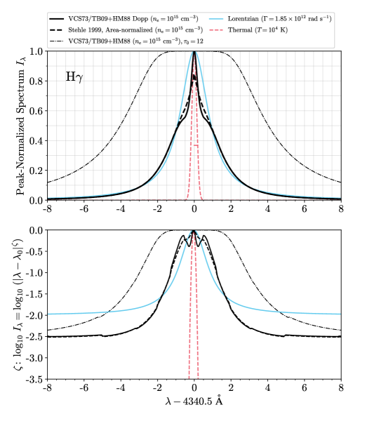
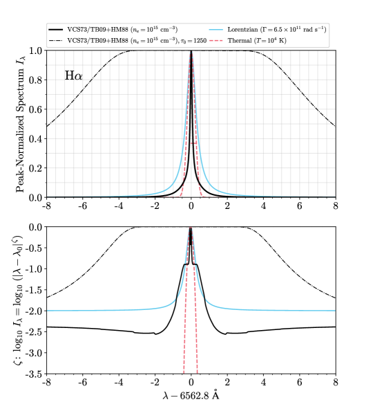
Figure 25: Optically thin spectral line profiles from the TB09$+$HM88 pressure broadening theory for Balmer H$\gamma$ (top two panels) and H$\alpha$ (bottom two panels) at $n_{e}\approx 10^{15}$ cm^-3. These are identical to the Vidal et al [746] (VCS73) calculations at this density, and they do not include thermal Doppler convolution in this figure. The 2nd and 4th panels show the slopes, $\eta$, calculated for each of the profiles in 1st and 3rd panels. Lorentzian profiles with scaled damping widths are overplotted for comparison. The slope of the H$\alpha$ pressure broadening profile is between the Holstmark and Lorentzian because of the higher importance of collisional broadening from electrons for this transition. The higher order lines, including H$\gamma$, are more obviously dominated by the quasistatic (Holtsmark-distributed) perturbations [cf. Fig 3 of 745], are less optically thick, are closer to LTE because of less scattering in this line, and are less affected by thermal broadening (the FWHM of H$\alpha$ is affected by thermal Doppler broadening even at such high densities; $1/e$ Doppler widths are indicated by horizontal red lines). The “self-broadening” of hydrogen is relatively less in H$\gamma$ and in the higher order lines, but it is important when the atmosphere is largely neutral [53]. The Balmer H$\gamma$ line is also less affected by thermal, $T=10^{4}$ K ion-dynamic effects [692]: we show an area-normalized (rather than peak-normalized) profile from [693], which includes additional Lorentzian damping near line-center from non-quasistatic components of the perturbing ionic field. Also shown are emergent spectral intensities (dashed-dotted black), with Doppler broadening included, from slabs with a physical depth of $dl=500$ m to demonstrate the large differences that result from curve-of-growth-like optical depth effects.

• H I$+$p⁺/e^-: “Stark broadening”, or electric pressure broadening of hydrogen, hydrogen-like ions, or Rydberg atoms by ambient charged particles (electrons, protons, ions) in the flare chromosphere, which is partially ionized by definition. The perturbations are caused by both electron collisional “damping” with a Lorentzian probability distribution and quasi-static splitting of energy levels from ambient positive charged protons (and ions) with a Holtsmark-like probability distribution. The splitting of energy levels is due to the first-order/linear Stark effect which is discussed in more detail in Appendix D. Optically thin emission line profiles from a homogeneous slab exhibit a Holtsmark power-law slope ($\log_{10}I\propto\log_{10}\mid\Delta\lambda\mid^{-5/2}$) in the far wings, if non-ideal effects are not important.

• LEPT: [556] discuss the role of broadening of hydrogen lines due to chromospheric plasma turbulence. Power-law electron beams drive a cospatial drifting return current, whose speed may exceed the threshold for the ion-acoustic / current instability and therefore lead to the development of ion-acoustic turbulence in the chromosphere (E. Oks, priv. communication 2022). The low-frequency electrostatic plasma turbulence (LEPT) is broadband, and it is quasi-static compared to radiative timescales. LEPT is treated as a statistically independent broadening process to the ionic microfield broadening and is therefore convolved with the Holtsmark or Hooper distribution of field strengths that enters into the nominal hydrogen line broadening (above). [556] analyzed several archival dMe flare observations of the Balmer series. Without detailed wing shapes, the values of FWHM/$\lambda_{0}$ from the data are degenerate with either electron densities of $>10^{15}$ cm^-3 or rms LEPT fields of $10-30$ kV cm^-1. Lower electron densities combined with LEPT development in the chromosphere are favored by considering the Balmer flux decrements or the last resolved Balmer line. Profiles dominated by LEPT have an exponential dependence in the far wings, $I\propto exp(-k\mid\Delta\lambda\mid^{\gamma}),\gamma\approx 1$.

• non-H$+$e^-, non-H$+$H: Collisional broadening of non-hydrogenic lines due to collisions with ambient electrons (the quadratic Stark effect) or with neutral hydrogen atoms [van der Waals broadening or the more complete ABO theory; 18, 52]. The quadratic (second order) electron impact damping of resonance ion lines, such as Ca II H and K, causes a small wavelength shift and a broadening that is typically $10^{3}$ smaller than the linear effect in hydrogen. The passage of H atoms is relatively fast and so this is a damping. non-H$+$non-H: Collisions among like atoms or ions results in resonance broadening. This is an exchange and thus described as a lifetime broadening effect (Bohm 1951). Optically thin emission line profiles have a Lorentzian shape (or Voigt if a Doppler broadening is included).

• HI$+$HI: Collisional damping of hydrogen lines from transient perturbations from other hydrogen atoms. van der Waals and resonance forces, collectively known as self-broadening, drop off rapidly with distance and so this interaction has a short duration. The neutral fraction of hydrogen is too small, even at $\sim 50$%, in the flare chromosphere for self-broadening to be significant in comparison to broadening by charged particles, unlike in the quiet Sun photosphere [53]. Optically thin emission line profiles have a Lorentzian shape (Voigt if thermal Doppler included).

• Thermal Doppler broadening is important for line opacity near $\lambda_{o}$ but decreases precipitously according to the Gaussian distribution. Note that one Doppler width is $\approx$ 0.2 Å for H$\gamma$ at $T=10,000$ K. Thus thermal Doppler broadening cannot explain broad wing emission unless there are very high temperatures $T\ggg 10,000$ K. Optically thin emission line profiles exhibit a Gaussian profile.

• Microturbulence, or nonthermal Gaussian Doppler broadening. An ad hoc microturbulence parameter is often used to account for missing broadening sources when all other known broadening sources have been exhausted. This parameter enters into the opacity (extinction coefficient) through a convolution of a Gaussian with the thermal Doppler core. (Certain values of this parameter may propagate through decades of stellar models with little critical reconsideration of their physical meaning or necessity.) For recent use in solar flare modeling of Fe II and Mg II lines, see [418] and [799], respectively. Non-Gaussian microturbulence is discussed often in the interpretation of solar flare transition region lines [194], but the densities are rather large and the optical depths are non-negligible even in transition region lines of quiescent state of active stars [e.g., 485]. [567] report nonthermal broadening velocities of several tens of km s^-1 in transition region flare lines with a temperature dependence, such that N V ($T>10^{5}$ K) does not exhibit excess broadening.

  Does the microturbulence parameter represent bona-fide gas-dynamic turbulence (eddies, vortices, random gas motions) in the footpoints of a flare loop [e.g., 79], and if so, through which fluid instabilities (e.g., Kelvin-Helmoltz, Rayleigh-Taylor) does the flare turbulence occur? The turbulence hypothesis can be investigated by considering the energetics inferred through spectral lines and the emission line flaring area on the star (see Sect. 12). [303] reported very broad, symmetric wings of Mg II h and k emission that had a small, bulk blueshift during a NUV flare observed by the Hubble Space Telescope/STIS. The wings would require electron densities as high as $10^{17}$ cm^-3 if due to collisional broadening. A Gaussian fit to the broad wings gives the line-of-sight velocity component root-mean-square (rms), $\sigma_{\rm{los}}$, and the kinetic energy of the chromospheric turbulence is

  $$KE=\frac{3}{2}\sigma_{\rm{los}}^{2}\rho_{\rm{chrom}}\Delta z_{\rm{chrom}}A_{\rm{flare}}$$ (22)

  where $A_{\rm{flare}}$ is the projected area on the star (Section 12) that produces the emission line flux at Earth. In this flare, the turbulence would be highly supersonic (200 km s^-1) and its kinetic energy would be several orders of magnitude larger than the radiated NUV energy.

• Opacity broadening, optical depth effects: It has long been known that simultaneous modeling of electron density and optical depth is required to interpret the hydrogen lines properly in stellar and solar flares [e.g., 193]. Optical depth effects cause a type of macroscopic broadening in chromospheric flare lines in the emergent spectral lines from stellar atmospheres. Sometimes this is loosely referred to as opacity broadening, which is described in [775], [605], and [294]. Essentially, opacity broadening follows from the Eddington-Barbier relation for a depth-dependent source function over optically thick wavelengths of a line. If the source function decreases in the outer layers a central reversal can form due to an absorbing layer for very optically thick lines; this is also sometimes called “self-absorption”. An optical depth broadening effect that is closely related to opacity broadening occurs in the enhancement of the emergent intensity at wavelengths that correspond to the transition from a formation over very large optical depths (where there is opacity broadening, proper) to smaller optical depths in the far wings. This is similar to the broadening in textbook illustrations of the curve-of-growth of a spectral line, whereby the Doppler core saturates at the local source function, and the Lorentzian or Holtsmark wings are very prominently in emission but are not close to saturation. The core saturation and wing enhancements of H$\gamma$ and H$\alpha$ are demonstrated in Fig. 25 for a slab thickness of $dl=500$ m and electron density $n_{e}=10^{15}$ cm^-3. An analysis of these effects in a heterogeneous, non-equilibrium model chromospheric condensation is presented in Kowalski et al [421]. [527] analyze in detail the self-absorption and pressure broadening in stellar flare H$\alpha$ emission lines.

• Red-wing and blue-wing asymmetries cause an increase in the breadth of a spectral line, especially if the line is spectrally and/or spatially unresolved. In stellar flares, red- and blue-shifted components of H$\alpha$ have maximum line-of-sight velocity extents of $\approx 100-300$ km s^-1 from the rest wavelength [743]. Reports of line asymmetries in the literature attribute the asymmetries to a variety of phenomena that involve chromospheric mass motions: beam-generated impulsive phase chromospheric condensations, coronal rain (a “coronal condensation”) from post-flare loop plasma draining and cooling to transition region and chromospheric temperatures, cool filament eruptions of plasma, absorbing downflows, and chromospheric evaporation of cool material into magnetic loops [see 784, for an overview]. Many stellar flare observations, however, with echelle resolving power have rather long exposure times ($t_{\rm{exp}}\approx 15$ minutes), and some are serendipitous single-exposure observations from exoplanet radial velocity monitoring. Additionally, optical depth effects and other microscopic broadening sources are important for interpretation. Optically thin emission lines can exhibit a velocity “smearing” in the emergent spectra, simply due to an integration of the emissivity over the velocity gradient along the line-of-sight, and optically thick lines are complicated by opacity broadening [527, 784].

  There are many reports of line asymmetries in hydrogen, helium I, and metallic lines throughout the UV, optical, and NIR that have been interpreted with these phenomena. The spectral observations consist of a bright emission line component around the rest wavelength and a fainter asymmetric wing component, or more than one wing component. Most modeling of these lines uses linear superpositions of Gaussians to characterize the shifts and widths of each component. [784], [529], and [531] use Voigt/Lorentzian profiles to isolate a Gaussian fit to a red-shifted components in large stellar flares. The bottom panel of Fig. 22 demonstrates this method, which effectively isolates a $\approx-100$ km s^-1 blueshifted component in the H$\alpha$ line flux during the decay phase of a white-light flare [552]. [197] and [241] report broad H$\alpha$ lines that are blueshifted during the rise and peak spectra during flares on UV Ceti and CN Leo, respectively. In the event on CN Leo, the blueshifts were -10 to -20 km s^-1 and the Gaussian FWHM values were 4.8 Å; the event on UV Ceti produced a similar width but a larger blueshift of -70 km/s. [243] presents detailed line profiles at high-time resolution during flares on Proxima Centauri with VLT/UVES. [741] and [743] discuss blueshifts observed across the Balmer series with some temporal resolution. [552] present a large survey of echelle spectral observations of the H$\alpha$ and H$\beta$ lines in M dwarf flares; the spectra had relatively short exposure times and were complemented with simultaneous optical broadband photometry, allowing the changes in the profile shapes to be characterized in the context of the impulsive and gradual phases of the white-light response (e.g., Fig. 22(bottom)). [321] report on high-time cadence monitoring of EV Lac and present persistent blue-wing asymmetries through the entire duration of a flare [see also 474]. [530] discuss a transient blueshifted H$\alpha$ absorption feature, while [529] analyze broad H$\alpha$ emission lines with red-shifted components, in flares on the young, solar-type flare star EK Dra, and Lalitha et al [434] analyze the redshift evolution of a broad H$\alpha$ line component in a flare on the K0Ve star AB Dor. [288] discuss blueshifted emission components in AT Mic. Of course, the location on the stellar disk is generally unconstrained in stellar flares, and the inferred velocities are not corrected for line-of-sight effects for field-confined flows, contrary to what is possible for solar flare observations [93].

  Flux-weighted line-center redshifts in Si IV and C IV during and after the impulsive phase of several dMe flares were reported in [302]. Chromospheric-line, red-wing emission in H$\alpha$, Na I D, and He I 5876 Å was described in Fuhrmeister et al [239]. These observations were tested against scaling relations (e.g., Eq. 3) from analytic models of impulsive-phase chromospheric condensations [220]. Late-phase redshifts, on the other hand, are usually interpreted as condensations that are analogous to the draining of cool material from the post-flare loops on the Sun. [784] discuss evidence from the time-evolution of the broadening of the H$\alpha$ line that could favor beam-generated condensations in the late-phase instead (which we note would be more in line with the multi-thread RHD modeling of the continuum radiation in the decay phase of large flares; Sect. 12, Fig. 30). [241] and [371] report on red wing enhancements in He I 7065 Å and 10830 Å emission lines, respectively, in two flares. [245] show remarkably broad He I 10830 Å wings during a flare on the dM3e star EV Lac; correspondingly broad H$\alpha$ profiles were analyzed in [244] and consist of a spectrally unresolved red wing satellite component. [465], [237], and [235] report redshifts in other transition region lines, such as C II, from low-mass stellar flares. [453] and [43] analyze the profile variations in FUV lines during flares on AU Mic and EK Dra, respectively. The optical Balmer lines have been decomposed into “separate” broad and narrow components, which exhibit clearly different Doppler shifts in some flares [326, 331, 241, 408]. Extreme blueshifted [328] and redshifted [777, 77] emission has been reported out to several 1000 km s^-1 in chromospheric and transition region lines. [398] discuss blueshifts and redshifts in a large sample of galactic field stars at larger distances and over a wide range of spectral types.

• Macroturbulence is a term that refers to a superposition of several Doppler-shifted profiles that originate from sequentially-ignited, neighboring flare loop footpoints, as in a solar arcade. The superposition is intended to emulate spatially unresolved flows, which are termed ‘directed mass motions’ in the literature. The unresolved flows may be preferentially blueshifted, preferentially redshifted [641], or equally blueshifted and redshifted [177]. To generate symmetric wings, the emergent radiation from downflows (e.g., a condensation) would have to precisely balance the emergent radiation, and thus the optical depths, from the upflows (e.g., evaporation) in neighboring loops. This precarious balance would have to be maintained over long durations, as for typical exposure times of $60-300$s. The lineshapes may take on a variety of symmetric or asymmetric forms that depart from Holtsmark and Lorentzian wing profiles.

10.2 Symmetric Wing Broadening of H Lines

The symmetric (or very nearly symmetric) wing broadening of hydrogen Balmer lines is a remarkable property of stellar flares. Full widths at 10% maximum in emission line spectra are as large as $\approx 15-20$ Å [297, 527]. The source of the symmetric broadening has been debated as a superposition of directed mass motions (macroturbulence), gas turbulence (as represented by a microturbulence parameter), and pressure broadening due to the Stark effect (Sect. 10.1). [177] and [197] argue against the Stark effect in the large dMe flares that they analyze by comparing to the optically thin wing predictions of Holtsmark profiles and the [746] profiles for electron densities of $n_{e}\approx 10^{15}$ cm^-3 [see also 330, 331, 287]. The better fits with multiple Gaussian components in these studies support the hypothesis of some type of supersonic laminar- or turbulent-emitting flows. The latter corresponds to a microturbulence parameter of $50$ km s^-1 around line center and $150-600$ km s^-1 in the wings. [508] present similar two-component Gaussian fits to broad and narrow components in H$\alpha$ and H$\beta$ in flares from the K dwarf LQ Hya; the broad components show relative shifts with respect to the narrow components and are interpreted in terms of various types of unresolved mass motions.

The alternative hypothesis for the source of the broad wings of hydrogen lines is pressure (linear Stark) broadening from ambient charged particles, which imprints unique signatures in the observations. Namely, the pressure broadening of hydrogen produces larger widths for larger $n_{j}$ within a series (e.g., within the Balmer, Paschen, or Lyman series) in the absence of optical depth effects and heterogeneities (here, $j$ refers to the upper level of a transition). However, the smoking gun signature is generally thought to be broader hydrogen emission line wings compared to nearby resonance lines of metallic ions, such as Mg II and Ca II, which experience a much smaller amount of broadening due to collisions with charged particles [170, 171]. [297] and [251] present much broader Balmer series lines in comparison to the Ca II K emission line [see Fig. 4 of 251] in the impulsive phases of two large dMe flares [see also 434].

We show two remarkable examples of the hydrogen broadening in stellar flare spectra in Fig. 26. The spectral broadening and emission line shape differences among Ca II K, H, and Balmer H$\epsilon$ ($n_{j}=7\rightarrow n_{i}=2$) are clearly evident in these echelle spectral observations. The top panel shows a serendipitous flare spectrum ($t_{\rm{exp}}=30$ min) from the inactive dM3.5-4 star Gl 6l 699 (Barnard’s star) that was studied in detail and modeled with the RADYN and MULTI codes in [579]. The bottom panel displays a sequence of spectra during a flare from the dM4.5e YZ CMi at the same times as shown for the H$\gamma$ spectra in Fig. A.1, top panel, of [743]. The inactive M-star flare shows some qualitative similarities to the line broadening in the spectrum of the decay phase of the continuum in the YZ CMi flare. These similarities are remarkable given that the stars have very different ages ($>7$ Gyr vs. $<500$ Myr, respectively) and quiescent magnetic activity levels. The impressive FUV flaring activity of Barnard’s star has been reported recently in [235]. A detailed analysis of the H9 Balmer line was presented for the large flare on CN Leo in [241]. Broadened Paschen lines have been reported in the decay phase of a large flare from the very low mass star VB10 [371]. Similar comparisons are, in principle, possible with the broadening of the high-order Paschen series and the Ca II infrared triplets [536], for which opacity broadening is perhaps less of a concern in comparisons to Ca II H and K.

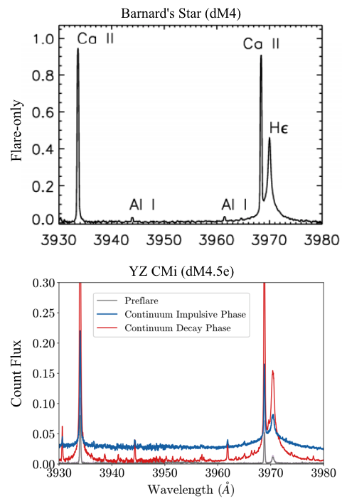
Figure 26: Dramatic broadening differences between hydrogen and metallic emission lines, such as the Ca II resonance lines, in flare spectra are considered evidence for the important role of pressure broadening of hydrogen. The pressure broadening of hydrogen constrains the charge densities (and optical depths) in the flare chromosphere. This conclusion is supported by detailed spectral synthesis with, e.g., the RADYN, RH, MULTI codes. The top figure shows these effects during a flare on the dM4 star Gl 699, reproduced from Paulson et al [579], and the bottom panel shows the coarse temporal evolution of the broadening differences during a flare [743] on the dM4.5e star YZ CMi.

10.2.1 Recombination Edge Modeling

Accurate interpretation of stellar spectra from EUV through NIR wavelengths depends on modeling how the wings of the hydrogen lines overlap and merge near bound-free ionization limits [338]. Accurate modeling, which should lack any sharp edge feature, opens up diagnostic power from the rich spectral region at wavelengths just longward of a recombination limit. For example, the Inglis-Teller relation is [355, 644]

$$\log_{10}n_{e}=23.2-7.5\log_{10}n_{\rm{max}}^{\rm{Balmer}}$$ (23)

which has commonly been used to determine electron density from the last discernible Balmer emission line near the Balmer recombination limit [430, 297]. Besides stellar flares, many types of astrophysical and laboratory phenomena also lack discontinuities in spectra around the expected location of hydrogen recombination edges [312, 209, 497, 677]. In solar flares, features such as a “blue continuum bump”, a shift of the edge to redder wavelengths, or a completely flat continuum have been reported in observations [533, 173]. The complete lack of any type of edge feature, and a lack of a jump in flux across the expected edge location, is ostensibly an indication of blackbody radiation.

However, the lack of an edge is also expected from recombination theory that includes non-ideal, level dissolution. The fundamental question pertaining to stellar flares is thus if there is enough instrumental blending of the wings and/or overlapping, linearly-superposed wing opacities to account for the lack of the observed discontinuities. A remarkable example of stellar flare spectra with no edge feature is shown in Fig. 11(a). Instead, these spectra (and others) show a series of faint, broad hydrogen lines that fade into a continuum. Other spectra, albeit at much lower resolving power, show some noisy features here, however [297]. Ostensibly, the conservation of oscillator strength density should result in a smooth transition of observed flux from a pseudo-continuum of a confluence of high-order, highly broadened and blended emission lines to the onset of recombination radiation. A phenomenological description of the transfer of bound-bound opacity to bound-free opacity was developed by [154] using the occupational probability ($w_{n}$) formalism in the non-ideal equation-of-state of [348]. The “dissolved-level” bound-free Balmer continuum opacity longward of the Balmer edge has been recently incorporated into spectral models of stellar flares [418, 408]. However, self-consistent modeling of the pressure broadening of the bound-bound Balmer lines [721] was not also included in the first models [415]. This incorrectly supported the extremely dense chromospheric condensations in 1D RADYN models (Sect. 8.2) as realistic models of flare density enhancements at cool temperatures [416]. Otherwise, the dissolved-level continuum opacities have largely reconciled observations with models by explaining the lack of an edge around $\lambda=3646-3700$ Å and the range of observed pseudo-continuum properties in between the longer-wavelength, high-order Balmer lines at $\lambda=3700-4000$ Å. The non-discontinuous, transition of dissolved-level opacities at $T\approx 10^{4}$ K have apparently reconciled the hydrogen recombination (Balmer jump) theory of the NUV with the blackbody-like theory of the optical continuum radiation.

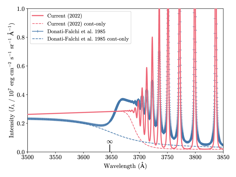
Figure 27: Direct comparisons of two methods [173, 418] for calculating the Balmer jump spectral region in solar and stellar flares. The emergent LTE intensity is calculated from a slab with $n_{e}=3.9\times 10^{13}$ cm^-3. The method from [173] predicts a “blue continuum bump”, whereas the current treatment with occupational probabilities predicts an extension of the Balmer continuum intensity to wavelengths longward of the “ideal” recombination limit (indicated by an $\infty$ symbol) at $\lambda=3646$ Å.

The physical cause of the continuous, dissolved-level opacity that was parameterized in [154] for hydrogen is still not well understood. Experiments with Rydberg atoms support the idea that Landau-Zener transitions [e.g., 802] at avoided level crossings [800, 640, 593] facilitate a cascading ionization process. In this picture, an electron is photo-excited to a high-lying level $n$ that is pressure-broadened to overlap with the broader, next higher-energy level $n+1$, thus effectively “dissolving” the level $n$. This description apparently explains the Inglis-Teller relationship through dynamic microfield ionization [348]. There are actually many types of calculations [455, 153, 64, 667, 59, 218, 219, 130, and see the review in Sections 86.2.2 - 86.2.3 in Drake 186, Weisheit and Murillo 766] that may contribute to “lowering the ionization potential” or “continuum lowering” in a hydrogen plasma with microfield fluctuations and collisional perturbations.

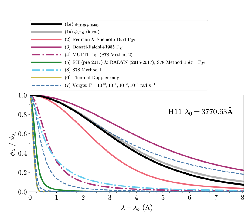
Figure 28: A variety of approximations to opacity line profile functions for the Balmer series have been used in stellar flare modeling codes over many decades. This figure summarizes the differences in models of the line profile function, $\phi_{\lambda}$, for the H11 Balmer line [see also 367, for a similar figure for the H10 line]. The calculations use $n_{e}=n_{p}=3.16\times 10^{14}$ cm^-3, or about 10x larger than in Fig. 27, and thermal Doppler broadening at $T=10^{4}$ K is included. The “ideal” profiles, $\phi_{VCS}$, are the VCS73 calculations from [443], and do not account for line narrowing due to occupational probability / level dissolution. Several Voigt profiles are also plotted for a range of Lorentzian FWHM values, $\Gamma$. Currently, the most accurate theory corresponds to the $\phi_{\rm{TB09+HM88}}$ (solid black) curve.

Due to level-dissolution in dense regions of flare atmospheres that are not very optically thick in the Balmer continuum, applying a simple relationship, such as the Inglis-Teller, that connects the last-visible hydrogen line to a single electron density may be misleading. [421] discuss a scenario wherein level-dissolution of hydrogen in a chromospheric condensation can generate an approximately grey opacity window at $\lambda\approx 3700-3750$ Å. Thus, the Balmer lines that are in emission in the emergent spectra actually originate from deeper layers with smaller ambient (thermal) electron densities and no apparent gas velocities. Due to the heterogeneous vertical stratification of the flare atmosphere, the high-order hydrogen Balmer series in emergent intensity spectra can be as broad as or less broad than the low-order Balmer lines (H$\gamma$, H$\beta$, H$\alpha$), which are very optically thick in some of the more recent RHD flare models. Some models of stellar flare spectra at the Balmer limit also incorporate spatial and temporal heterogeneity within the flare ribbons [408]. These seek to explain the inconsistencies in large $n_{\rm{max}}^{\rm{Balmer}}\gtrsim 15$ (Eq. 23) being observed (indicative of low electron densities, $n_{e}=10^{13}-10^{14}$ cm^-3) with the necessity to also produce the observed continuum properties from a location on the star with much larger electron density ($n_{e}\gtrsim 10^{15}$ cm^-3; $n_{\rm{max}}^{\rm{Balmer}}\approx 11$). Note that in occupational probability theory, however, there is not one single maximum upper level for all atoms in a plasma.

Fig. 27 directly compares two different modeling techniques within the Balmer jump spectral region. The emergent intensity is calculated in LTE from a static slab with $dl=400$ km, $T=10^{4}$ K, and $\rho=10^{-10}$ g cm^-3 ($n_{e}=3.9\times 10^{13}$ cm^-3). [173] modeled several solar flare spectra (with high resolving power) using Voigt profiles up to $n_{\rm{max}}=2\times 10^{4}T^{0.25}n_{e}^{-0.25}\approx 65-85$; this is a saddle-point estimate with Debye-screening of the proton field [499]. This method convolves the Balmer edge with the Voigt function corresponding to the line with $n_{\rm{max}}$. The “current (2022)” method uses the TB09$+$HM88 profiles [721] and the dissolved level bound-free continuum opacity. Many other various approximations for the pressure broadening of hydrogen have been used in models of solar and stellar flares. The ambiguities were discussed extensively in [367] and were resolved only in recent years. In Fig. 28, we summarize the wide variety of broadening prescriptions for the Balmer H11 line, whose integrated flux is sensitive to the amount of level dissolution in the densities of flare atmosphere models [415]. For a description of each method presented in the figure, we refer the reader to [421] where similar comparisons are shown for the Balmer H$\gamma$ line.

11 A Comprehensive Multi-Wavelength Stellar Flare Dataset

What fundamental physical parameters can one infer using a multi-wavelength dataset of a stellar (super)flare? A comprehensive analysis of a series of two consecutive superflares from the binary dM4e$+$dM4e system DG CVn was presented in [571], who summarize the plasma and geometric properties that can be constrained in a flaring atmosphere. This culminates an extensive history of stellar flare research, and we briefly review the salient points to the algorithm.

11.1 Inferring Nonthermal Electron Properties from Stellar Data

The nonthermal radiation from power-law electrons in stellar flares occurs as hard X-rays ($E\gtrsim 10$ keV) and as incoherent gyrosynchrotron radiation in the radio/microwaves at cm wavelengths. The radiative processes are thought to be similar to solar flares, in which the hard X-rays are emitted through collisional bremsstrahlung in the chromosphere, whereas the radio flux originates from predominantly higher energy electrons ($E\approx 100-300$ keV) trapped in magnetic fields; see the review in [772]. The distribution of electrons is parameterized in the hard X-rays and radio using two power-law indices, $\delta_{x}$ and $\delta_{r}$, respectively. From hard X-rays, the particle flux distribution is

$$F(E)=F_{o}\left(\frac{E}{E_{c}}\right)^{-\delta_{x}}$$ (24)

where $E$ is the electron kinetic energy in keV, $E_{c}$ is the low-energy cutoff, and $F_{o}$ is the differential (specific) electron flux density (el s^-1 cm^-2 keV^-1) around the cutoff energy. Similarly, a nonthermal electron beam density distribution determined from the radio is written as

$$n(E)=n_{o}\left(\frac{E}{E_{c}}\right)^{-\delta_{r}}$$ (25)

where $n_{o}$ is the differential number density (el cm^-3 keV^-1) of electrons around energy $E_{c}$. If the same population of electrons is responsible for both X-rays and radio, then $\delta_{x}\approx\delta_{r}$ is expected for electrons with velocity $v$ very close to the speed of light $c$; otherwise, $\delta_{x}\approx\delta_{r}-0.5$. The different forms (i.e.,, flux density vs. number density) of these equations is because the injected power-law flux distribution is inferred through the collisional thick target model of the hard X-ray spectrum, whereas a power-law density distribution is determined through observations at optically thin microwave frequencies (see below).

Note that the integral of Eq. 24 multiplied by $E$ gives the total beam energy flux density (erg cm^-2 s^-1), which is an important input for flare modeling (e.g., F10, F13, etc…). Integrating Eq. 25 over energy gives the total beam density, $N$, where $N$ is the quantity that is used in the gyrosynchrotron expressions in [195] if $E_{c}$ is set to $10$ keV. In the studies of [687, 571, 196, 195], Eq. 25 is integrated from $E_{c}$ to $\infty$ to replace our $n_{o}$ with the prefactor $N(t)\frac{\delta_{r}-1}{E_{c}}$ where $N(t)$ is the total electron density (el cm^-3) above the cutoff (and the same is usually done for Eq. 24). Eq. 24 can be multiplied by a probability density function for the angular distribution, $M(\theta)$, to specify the directivity of particles with respect to the magnetic field [11]. A highly-collimated Gaussian distribution is usually chosen for $M(\theta)$. Then, a “1.5D” solution to the Fokker-Planck equation (Sect. 9.2) accounts for the changes in the pitch angles of the particles.

The best diagnostic of accelerated particles in stellar flares is optically thin frequencies in the mm or radio. If the observations are in the radio at GHz frequencies, one must ensure that these frequencies are above the peak frequency ($\approx 10$ GHz) so as to be in the optically thin part of the gyrosynchrotron spectrum. An expression from [195] converts from a power-law index in the optically thin flux spectrum, $S_{\nu}\propto\nu^{\alpha_{r}}$, to the power-law index in the electron distribution, $\delta_{r}$:

$$\alpha_{r}=1.22-0.90\delta_{r}$$ (26)

The power-law index in the optically thick part of the spectrum is much less sensitive to the power-law index of nonthermal electrons.

Following [687], the kinetic energy of nonthermal particles can be constrained from the radio spectrum as follows. The power per volume in nonthermal electrons above the assumed low-energy cutoff value, $E_{c}$, is given by Eq. 9 of [571]. In this equation, the total number of nonthermal electrons, $N(t)V(t)$, over the flaring volume $V(t)$ is an unknown, but it is directly proportional to the optically thin spectral radio luminosity, $L_{\nu}$. By constraining the value of $\delta_{r}$ in this part of the spectrum and invoking some prior knowledge or assumption about the peak frequency, an integral over the entire radio spectrum can be calculated – including the optically thick part – to give the time-integrated energy of nonthermal electrons in the flare. This leaves one unknown, the magnetic field, $B$, in the gyrosynchrotron emissivity formula for the optically thin part of the spectrum (see below for further constraints on the magnetic field, but it must be assumed that the $B$ derived from the radio originates from the same $B$ that is derived from the soft X-rays). If the radio or mm data are available at only one frequency, and thus a spectral index cannot be determined from the data, then contours of nonthermal energies and plausible ranges of magnetic field strengths and spectral indices are reported, as in Fig. 29, which is reproduced from [571] [see also 471, where a spectral index was derived from mm observations].

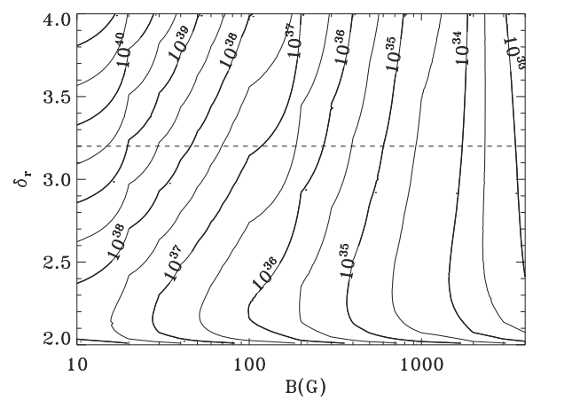
Figure 29: A range of possible nonthermal electron beam power-law indices and magnetic field strengths that can be constrained from gyrosynchrotron data of stellar flares; reproduced from Figure 6 in [571] with permission. See also [687] and [471]. Contours of constant electron beam kinetic energies add a third constraint. Cross sectional footpoint areas from optical data can constrain the beam flux density for forward modeling inputs [569, 571].

X-ray and optical data can constrain the physical parameters of flares further. From time-resolved X-ray spectra, one obtains the volume emission measure, $\mathcal{VEM}$. The $\mathcal{VEM}$ is $\int n_{e}^{2}dV$, which is the amount of optically thin emitting plasma at a fixed X-ray temperature, $T_{X}$. Typical values of the $\mathcal{VEM}$ (in M-dwarf flares) are $10^{51}-10^{52}$ cm^-3. In a $\log_{10}$ $T_{X}$ vs. $\log_{10}\ \sqrt{\mathcal{VEM}}$ diagram, the peak $T_{X}$ may clearly occur before the peak $\mathcal{VEM}$ [213, 34, 448]. Over the decay phase evolution of a flare, the slope in this diagram provides one of three inputs for the widely employed flare loop modeling of [607]. Combined with an exponential decay constant from the X-ray light curve and the maximum X-ray temperature, a semi-circular loop’s half-length, $l$, can be inferred. The loop sizes in giant X-ray flares are typically reported to be on the order of the stellar radius [e.g., 213, 569, 434, 571]. Note, large $50-200$ Mm loop lengths are also inferred under some interpretations of QPPs (Section 6.2) in optical broadband light curves [16, 184].

Optical and/or NUV data provide data to relax the geometrical assumption of a single, giant monolithic loop (Sect. 12), while also providing constraints on the electron density and the magnetic field strength in the flare corona. The optical and NUV probe the footpoint radiation, from which a dimensionless ratio of $R_{\rm{foot}}/(2l)$ can be calculated, where $R_{\rm{foot}}$ is an equivalent radius of the area of an optical flare footpoint: $A_{\rm{flare,opt}}=2\pi R_{\rm{foot}}^{2}$. By combining with an alternative expression for the $\mathcal{VEM}$ in terms of these quantities and using the value of the $\mathcal{VEM}$ from X-ray spectral fitting, a representative value of the coronal $n_{e}$ is readily obtained that is independent of the number of identical loops in a hypothetical stellar arcade [Eq. 25 of 571]. One also can assume that the magnetic pressure must be at least equal to the gas pressure of the evaporated MK plasma for it to be confined to the loops instead of cooling through expansion, as in a scenario analogous to a filament eruption or coronal mass ejection [145]. The magnetic field confinement condition places a lower-limit on the coronal magnetic field of the flaring loops.

[523] homogeneously analyzed a large sample of many sizes of X-ray stellar flares from various spectral types and evolutionary stages using “Haisch’s simplified analysis” [HSA; 292], which involve scaling relations [see also 731] that infer coronal temperature, electron density, loop length, and confining magnetic field strength from an emission measure and light curve decay timescale. Typical X-ray temperatures derived from multi-component fits to $E=0.5-10$ keV spectra are similar to those in solar flares, $T_{X}\approx 15-30$ MK [e.g., 567, 448, 527]. At the low coronal temperature end, $T\approx 2-15$ MK, electron density variations, or lack thereof, are constrained with X-ray spectra of the $f$ (forbidden) and $i$ (intercombination) components of helium-like triplets [e.g., bottom right spectra in Fig. 18; 283, 565, 708, 567, 448]. When significantly detected, the flare-enhanced electron densities are reported in the range of $10^{11}-10^{12}$ cm^-3 at these cooler coronal temperatures.

Osten et al [571] summarize the physical parameters in three of the largest dMe flares that have been observed with X-ray spectra (cf. their Table 5). The inferred temperatures are $T\approx 50$, $140$, $290$ MK; the electron densities are 3 $\times 10^{11}$, 3 $\times 10^{12}$ 3 $\times 10^{11}$ cm^-3; the confining magnetic field flux densities are 230, 1100, 580 G, respectively; and $\mathcal{VEM}$ ranges between $10^{54}-10^{55}$ cm^-3. Generally similar numbers are found in the largest RS CVn flares, which produce integrated X-ray energies and luminosities one to two orders of magnitude larger [568, 376]. YSO’s also exhibit such extreme volume emission measures and temperature [$40-80$ MK; 748]. These superhot temperatures correspond with X-ray luminosities that are close to or in excess of the bolometric luminosity of the star. Note that in an X-ray superflare from the dM3.5e star EV Lac with comparable temperatures ($T_{X,\rm{peak}}\approx 70$ MK) that were derived from the hydrodynamic modeling analysis of [607], [213] argue that accounting for the $E>10^{34}$ erg of energy release during the flare places further constraints on coronal magnetic fields in the $\approx 4$ kG range before the flare.

The peak stellar flare values of $\mathcal{VEM}$ and $T_{X}$ generally compare well with scaling relations over many orders of magnitude, from superflares to solar flares, in the famous “Hertzsprung-Russell (H-R) diagram of solar and stellar flares” [790]. The H-R diagram of solar and stellar flares was first theoretically explained using MHD scaling relations in [672]. This diagram was investigated further in [34], and the tightest correlation was reported in the empirical relationship

$$\mathcal{VEM}(T_{p})=10^{50.8}\big{(}\frac{T_{p}}{\rm{10\ MK}}\big{)}^{4.5\pm 0.4}[cm^{-3}]$$ (27)

where $T_{p}$ is the peak flare X-ray temperature. Their relation for decay time and peak temperature is, in principle, useful for inferring physical parameters if only the decay phase is caught in the observations [43]; however, the empirical scatter about the trends is an order of magnitude in both quantities. [257] and [571] suggest that the hottest ($T_{X}>100$ MK) stellar flares exhibit a “saturated”-like volume emission measure of $\approx 10^{55}$ cm^-3 and do not follow a solar extrapolation in the flare H-R diagram. [672] include two additional parameters (either loop length or magnetic field and ambient thermal electron density) in their scaling relation analogue [see also further alternatives summarized in 309] to Equation 27 to explain the apparent offset in volume emission measure from the solar extrapolation. [335] include a much smaller flare from an active M-dwarf flare in the context of stellar superflares and solar flares. [571] report on a stellar superflare (their “F2” event) with $T_{X}\approx 50$ MK that is within a factor of 2.5 in the predicted $\mathcal{VEM}$ given by Equation 27.

Large stellar flares occasionally trigger Swift’s Burst Alert Telescope (BAT trigger numbers 172969, 310125, 331592, 596958, 625898), which is intended to automatically slew to gamma-ray bursts and other extra-galactic transients. The combination of X-ray data from the BAT and at softer X-ray energies from the Swift’s XRT facilitates classical model hypothesis testing among thermal and nonthermal models out to $E\approx 100$ keV. In superflares from II Peg and DG CVn, nonthermal bremsstrahlung models were found to be equally statistically robust fits as a superhot thermal model fit. However, in the superflare event from DG CVn [571] that the BAT spectra triggered on, the $T_{X}=290$ MK thermal model was favored over a nonthermal model because the time-evolution of the X-rays was delayed with respect to the optical $V$-band data [in line with the thermal, empirical Neupert effect; 108], and a footpoint area from the optical gives (even by stellar flare standards) unrealistic collisional thick target electron beam energy and flux into the lower atmosphere. The collisional relaxation times were estimated to be rather short compared to the (classical) thermal conduction times, thus further supporting the thermal interpretation. Additional evidence for thermal interpretation of superflare X-ray emission from YSO’s is discussed in Vievering et al [748].

In soft X-ray flare spectra, features around the Fe 6.4 keV K$\alpha$ emission line and the 6.7 keV Fe XXV thermal emission line complex are also reported. These features have been interpreted as either electron beam excitation [202] or non-LTE fluorescence of a larger-area photospheric ‘halo’ [568, 192, 569]. However, there are some calibration issues in Swift data around these features that have been reported only recently [572]. The recalibrations greatly diminish the 6.4 keV feature while enhancing the 6.7 keV complex. Fe K$\alpha$ fluorescence was studied in a flare from an active giant star using a different observatory (Chandra) without instrumental problems and higher resolving power [710]; see Sect. 12.2.

Table 8 highlights a few important multi-wavelength diagnostics in stellar flares that have been discussed in this review. Of course, the interpretations of these diagnostics are complicated by issues pertaining to heterogeneities of the unresolved nature of stellar flare sources (in time, and in all three spatial directions), and thus are generally model-dependent. In the final section of this review, we discuss assumptions for and inferences of stellar flare geometries and the associated implications for heterogeneity.

Table 8: A summary of flare diagnostics

Measurement/Data	Physical parameter of flare
X-ray exponential decay constant, $T_{X,\rm{max}}$, slope in $T_{X}$ vs. $\mathcal{VEM}$	semi-loop length $l$
Slope at optically thin radio/mm frequencies	power-law index of NT electrons, $B$, $E_{\rm{NT,kinetic}}$
Optical ($\lambda>4000$ Å) color temperature	Footpoint area
Optical or $U$-band light curve timing vs. X-rays, impulsiveness index	non-thermal vs. thermal interpretation of hard X-rays
Balmer jump ratio (or H$\gamma$/C4170′)	Optical depth at $T\approx 10,000$ K
H$\epsilon$, H$\delta$, or H$\gamma$ vs. Ca II H or K	electric pressure (Stark) broadening vs. turbulent Doppler broadening
Fe K$\alpha$ spectral region	fluorescence vs. NT/beam excitation, viewing angle, halo geometry
$f/i$ ratios from X-ray spectra of helium-like triplets (e.g., O VII $\lambda\approx 22$Å)	thermal electron densities at $T\lesssim 15$ MK

12 Stellar Flare Geometries

Stellar flares are spatially unresolved point sources. Yet, from spectral data, model fitting, and sufficient time-resolution, there are many properties of the spatial dimensions of flaring sources that can be inferred. These reveal similarities to solar flare phenomenology at similar wavelengths and strongly reinforce the solar-stellar connectivity of flare physics. In this section, we review the methods and results of stellar flare geometry calculations.

Optical and NUV observations constrain the chromospheric/photospheric flare areas. A blackbody temperature, $T_{\rm{flare}}$, and the fraction (“filling factor”) of the visible stellar hemisphere that is flaring, $X_{\rm{flare}}=R_{\rm{flare}}^{2}/R_{\rm{star}}^{2}$, can be fit to spectral data or multi-band photometry through the following equation [298, 302]:

$$f_{\lambda,\rm{Model}}^{\prime}=\Big{(}\pi B_{\lambda}(T_{\rm{flare}})-S_{\lambda,q}\Big{)}X_{\rm{flare}}\frac{R^{2}_{\rm{star}}}{d^{2}}$$ (28)

where $B_{\lambda}(T_{\rm{flare}})$ is the Planck function intensity model of the flare, $S_{\lambda,q}$ is the surface flux of the quiescent star, and $f_{\lambda,\rm{Model}}^{\prime}$ is the ‘flare-only’ model flux at Earth above the atmosphere that is to be fit to the observed, calibrated [erg cm^-2 s^-1 Å^-1] flare-only flux, $f_{\lambda}^{\prime}$. The ratio of flare-only fluxes at two wavelengths is a flare color and is the minimum information that is needed to solve for $T_{\rm{flare}}$ in Eq. 28 (through linearization and iteration or a lookup table). An $m$-component, linear superposition of RHD surface flux flare spectra, $S_{\lambda,\mathrm{RHD},m}$, or a multi-thermal blackbody model are typically required to reproduce the optical and NUV continuum observations over a wavelength range spanning more than $\Delta\lambda\approx 1000$ Å. Additional terms are thus included in Equation 28. For an $m$-component RHD model superposition, the solution is a linear least squares fit to an observed flare-only spectrum, $f_{\lambda}^{\prime}$, resulting in the estimated parameters, $\hat{X}_{\mathrm{flare},m}$ [see 571, 418, 408]. For further discussion, see Appendix C.

Constraints on $X_{\rm{flare}}$ from blackbody fitting to optical flare-only spectra result in inferences that a small fraction of the visible stellar hemisphere flares for even the largest, $E\approx 10^{34}$ erg, dMe events. For example, the broadband photometry in the Great Flare of AD Leo [297] constrain $X_{\rm{flare}}$ to be 0.5% [295] in the first impulsive peak. Fits to the flare-only, optical continuum in the rise/peak spectrum of this event are consistently small (0.2%) but with a correspondingly larger blue-optical blackbody color temperature of $T_{\rm{flare}}\approx T_{BB}=11,600$ K [414]. An $m=2$ component RHD model of this spectrum gives a similar filling factor for a model with large electron-beam heating fluxes, which are combined with the second RHD model component with filling factors that are $\approx 2-10$x larger in order to account for most of the narrow emission line flux [408, see also Cram and Woods 140, Hawley and Fisher 295, Kowalski et al 412]. The corresponding projected area at the star is $A_{\rm{flare}}=X_{\rm{flare}}\pi R_{\rm{star}}^{2}$, which may instead consist of a series of $K$ circular flare kernels. Inferences in smaller dMe flares from broadband photometry [302] and optical spectroscopy [416] are consistent with very small areas $\approx 5-10\times 10^{16}$ cm², thus reinforcing the analogy to compact white-light kernels that are observed at the footpoints of impulsively heated loops in solar flares [e.g., 231]. During the most energetic dMe events, however, peak-phase flare areas are inferred to be several orders of magnitude larger than solar flare white-light and NUV areas [425, 417].

In the gradual decay phase, and in the impulsive phase of gradual-type dMe flare events with large Balmer jump ratios, blackbody fits to broadband photometry may be misleading (Sect. 7.2.4). Blackbody fits to the gradual phase continuum give a rather inconsistent picture of the post-peak footpoint areal evolution from event to event; perhaps, heterogeneous RHD model superpositions in the gradual decay phase are much more important for accurate areal inferences than in the $10^{4}$ K blackbody-like rise and peak phase. A superposition of RHD model components in the gradual decay phase of a megaflare on the dM4.5e star YZ CMi is shown in Fig. 30 from [418]. This model was previously developed to explain the NUV to $V$-band ratio in the DG CVn superflare event reported in [571], and it also adequately modeled the NUV continua and Balmer jumps in much smaller, gradual-type events [420]. This “DG CVn superflare multi-thread (F13) model” consists of several RHD model spectra over the evolution of the atmosphere that is shown in Fig.21, thus superposing snapshots from a range of optical depths, temperatures, and densities (see Sect. 12.1) in order to explain the gradual decay phase.

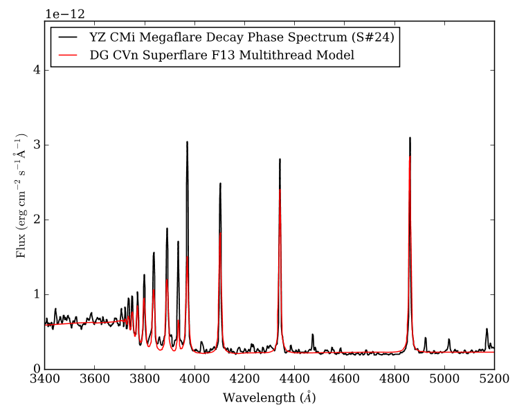
Figure 30: Gradual-decay phase, flare-only spectrum of a megaflare on the MV4.5e star YZ CMi [412]. Multi-thread RHD modeling of another superflare on DG CVn [571] adequately reproduces the Balmer jump, optical continuum shape, and some of the hydrogen Balmer emission line properties (but some important shortcomings remain). Each RHD model component is calculated self-consistently, but the linear superposition of the model components is semi-empirical; see discussion in [418] and [419].

Various size scales in solar and stellar flares are shown in Fig. 31.

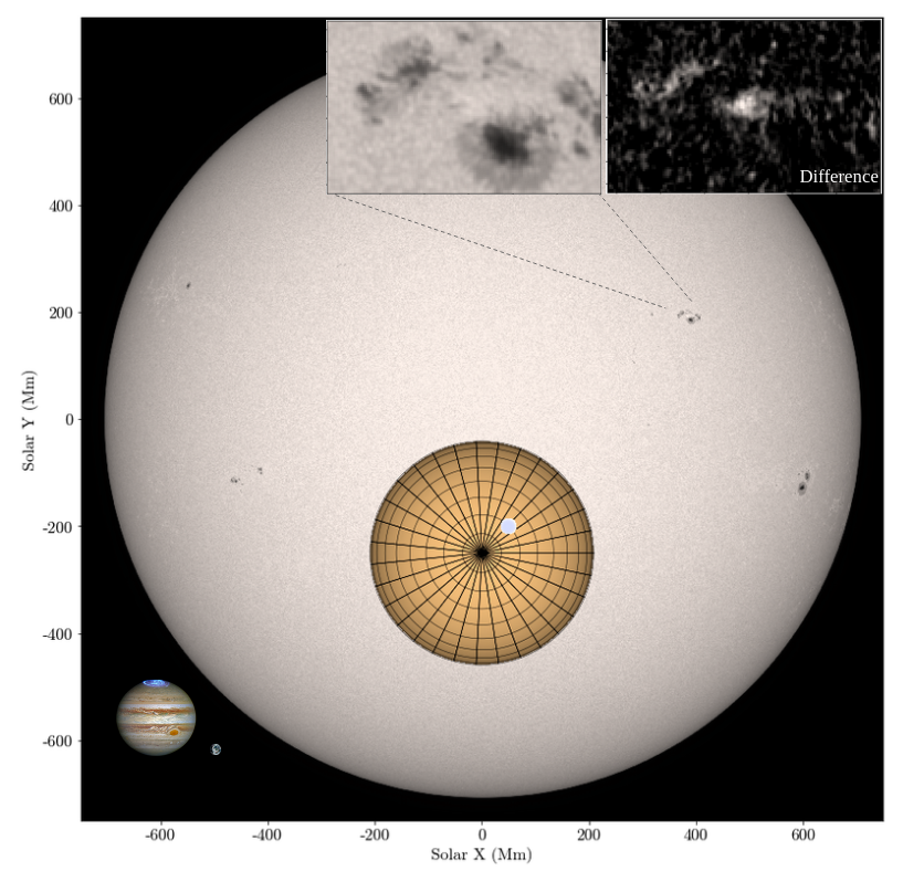
Figure 31: Sizes to scale. An image of the Sun at $\lambda=6173$ Å from the Helioseismic and Magnetic Imager [HMI; 652] on SDO, a representative size of an active mid-type (MV3e-MV4.5e) M star ($R_{\rm{star}}=0.3R_{\rm{Sun}}$), and a circular flare area ($\approx 5\times 10^{18}$ cm² ) that corresponds to about 0.5% of the visible hemisphere of this hypothetical M star. For comparison, Earth and Jupiter are shown to scale. The insets each have a field-of-view of $\approx 10^{19}$ cm², and they show an image of the solar active region in the NW quadrant during the hard X-ray impulsive phase of the SOL2014-03-29T17:48 X1.0 flare (total intensity left, difference image right). For a detailed analysis of the HMI data of this solar flare, we refer the reader to [392]. Jupiter image credit: NASA, ESA, and J. Nichols; Earth image credit: GOES/NOAA/NESDIS.

12.1 A Dominant Loop or an Arcade?

There are two general approaches to modeling spatially unresolved flare light curves and spectra [448]. The first approach is summarized in [376], and references therein, where it is most recently applied to an RS CVn X-ray superflare. This modeling follows the analysis of [607] and describes the rise and decay of a flare as result of a dominant monolithic loop (or a superposition of a few dominant loops that are heated and cooled simultaneously). The heating and cooling timescales in the loop are on the order of tens of minutes to hours [see also 608, 709, 20]. In [608], the initial X-ray event in the same flare in Fig. 18 was modeled with this method, and the subsequent X-ray flare in the event was modeled as an arcade of $\approx$ five loops that were sequentially heated in a nearby region. Coincidentally, a solar analogy inspired a similar hypothetical explanation for the NUV and optical footpoint ignition during the decay phase of a different M dwarf flare in Kowalski et al 418. Longitudinal MHD oscillations in a monolithic, giant (200 Mm) loop have been proposed as an explanation for the triggering of quasi-periodic, $U$-band, light-curve oscillations in the decay phase of this megaflare event [16]. The comparisons of particularly dense snapshots [e.g., $t=2.2$ s; 415] from RHD models to observations also inherently make the assumption that a single dominant kernel at any one time contributes to the bulk of the flux received at Earth [but see 528, for recent tests of this assumption].

An alternative hypothesis is known as “multi-thread modeling”, which was pioneered by [324], [615], and [762] to explain Sun-as-a-star soft X-ray solar flare light curves. These works addressed the large discrepancy between the observations of long decay times in GOES soft X-rays and the very short decay times in models of individual loops; multithread techniques have further been used to model a variety of solar flare phenomena [e.g., 616, 642, 611]. Elements of this approach and of observations of sequential footpoint brightenings in the hard X-ray and optical wavelengths in solar flare ribbons [e.g., 405, 601] have inspired stellar flare RHD model superpositions [571, 418] for more direct comparisons to spatially unresolved observations. [258] argue that the rise phase of a giant X-ray flare from the PMS star DQ Tau consists of a multi-threaded source; see also [661] in reference to the modeling approach showcased in Fig. 23. Doyle et al [184] suggest that a series of tens of loops contribute to the geometrical dimensions, as inferred from their QPP (Section 6.2) analysis, in two high-energy flares. [487] discuss the loop triggering scenario of [201] as an alternative hypothesis for short-duration QPPs in white-light. [567] hypothesize that an arcade of heterogeneous gyrosynchrotron-emitting loops may explain the microwave spectral indices in a large dMe flare.

Multi-thread modeling approaches seek to be more representative of a solar flare arcade geometry, following arguments previously made in stellar [295] and solar modeling [296]. However, ad hoc geometrical assumptions and simplifications must be imposed due to the absence of appropriate (i.e., broad spectral coverage, high-time resolution, unsaturated data at comparable wavelengths) constraints from solar data. Recent analyses of IRIS solar data at high-time resolution, such as the “new area” calculations of [274], and spatially resolved spectral line analyses [528], may be able to provide clearer guidance to stellar models of sequential footpoint ignition. Nonetheless, there may be important differences between solar and stellar flares that complicate a direct application of the thermal multi-thread modeling of [762]: shorter-during footpoint pulses [e.g., 487], greater importance of the gradual-phase white-light continuum radiation [297, 309] and particle acceleration [567], and larger apparent loop height growth over the flare evolution [$\tau_{c}\propto l^{2}$; e.g., 567, 571] all are examples of properties that distinguish stellar flares.

Novel stellar flare applications of the two-ribbon solar flare reconnection model of [404] are described in [595] and Güdel et al 282 [see also 292]. [282] model the $\Delta t\approx 8000$ s rising phase of a flare on the RS CVn UX Ari in this framework. This flare exhibited a remarkable peak X-ray luminosity of $>10^{32}$ erg s^-1, and they infer the evolution of the reconnection heights and electron densities (which evolve through $\approx 10^{11}$ cm^-3 at peak). A long-duration decay phase is predicted by the model, and the paper discusses how the lack of nonthermal particles in the early rise phase is a potential limitation of the original assumptions.

12.2 Stellar Core-Halo

Multi-dimensional geometrical analysis of flare sources is possible by combining hydrodynamic modeling of loop lengths and high resolution spectral observations at Fe K$\alpha$. The technique is described in [710], who infer an X-ray source height that irradiates a large area of the photosphere, from which the Fe K$\alpha$ is observed at a viewing angle $\phi$. The geometry is shown in Fig. 32. The combined constraints from the Palermo-Harvard code and the MOCASSIN 3D Monte Carlo radiation code [207, 208, 191] are reproduced from their paper on the right of Fig. 32. Recently, Werner band H₂ flare emission has been reported in [235] and interpreted as fluorescence due to O VI $\lambda=1032$ Å irradiation of the temperature minimum region ($T\leq 1500$ K).

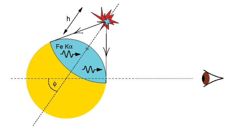
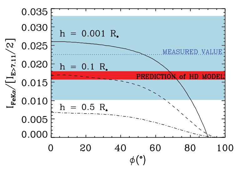
Figure 32: Geometrical inference from spectral analysis of the 6.4 keV (1.94 Å) Fe K$\alpha$ emission line during a flare on the giant star HR 9024, reproduced from [710] with permission. The X-rays from hot flare loops fluoresce the neutral iron in the surrounding photosphere. The modeling leverages hydrodynamic modeling from [709].

In 1D radiative-hydrodynamic modeling, XEUV backwarming of the photosphere is approximated using the treatments of [248], [295], [296] and [2] through exponential integrals and detailed radiative transfer [10, 753]. A multi-dimensional extension of UV and optical radiative backwarming is illustrated in a cartoon of Figure 4 of [225], and the geometrical dilution of chromospheric radiative flux impinging on the photosphere is given by their Eq. 25.

The remarkable, state-of-the-art 3D MHD codes that have been recently developed with the primary goal to study quiet Sun magnetism are not ready to address some of the most pressing current problems in stellar flare physics. Flare models require accurate treatments of non-equilibrium physics and detailed radiative transfer for comparisons to chromospheric observations. An approximation to nonthermal particle heating can in principle be included as $Q_{\rm{flare}}$ in the energy equation in 3D simulations of small flares [236]. The geometrical grid spacing in 3D MHD models, however, is immobile and too coarse (e.g., see Sect. 8.2) to resolve the gradients and contribution function features for the optically thick spectral lines and continua. Section 4.6.1 of [76] discusses the issues facing a 3D MHD solar flare simulation that predict chromospheric emission lines in response to thermally conducted fluxes. The RADYN code (for example) was originally a “quiet” Sun code, but it had implemented the 1D adaptive grid scheme of [175] and was flexible enough to simulate particle beam heating in a non-solar gravity. These features proved fortuitous in applications to stellar flare models. The stellar community is in urgent need of collaborative development of multi-dimensional extensions of Carlsson’s and Dorfi’s works, such as [699], in order to understand the comprehensive, radiative-hydrodynamic response of stellar atmospheres to the impulsive release of magnetic energy.

13 Conclusions and Future Outlook

In conclusion, we summarize six, non-exhaustive big-picture questions that are (in our view) at the forefront of stellar flare research.

• Stellar flares routinely attain energies and peak luminosities that are factors of $10^{2}-10^{4}$ greater than the largest solar flares. How are the flare energies connected to photospheric magnetic flux densities/geometries, particle acceleration properties, flaring footpoint areas, and energy transport processes in the atmospheres of other stars

• Stellar superflares exceed the quiescent bolometric stellar luminosity. The rate of superflares, however, is not characterized with high statistical significance. What are the rates of events in the superflare regime for solar analogs and other low-mass cool stars as a function of stellar age?

• On the Sun, the brightness of chromospheric flaring sources is transient at any single location for (arguably) $\lesssim 10-20$ s. A comprehensive, self-consistent model (e.g., within frameworks similar to Reeves and Forbes 614 and Rempel et al 623 pertaining to solar flare soft X-rays) has not yet been developed for optical or radio stellar flare light curves that last for tens of minutes to hours. What are the principal physical parameters that drive the observed temporal scales of stellar flare light curves of optically thick radiation in the rise and decay phases?

• Blue asymmetries in Balmer lines are often interpreted as evidence of mass eruptions from a star. Are there direct analogues [e.g., as in Mg II; 707] on the Sun, and does chromospheric evaporation in stellar flares contribute to blueshifted spectral features in cool lines?

• Turbulent mass motions and other non-equilibrium macroscale processes (e.g., UV and X-ray radiative backwarming) in stellar flares remain poorly understood in three spatial dimensions. If gas-dynamic turbulence is important for explaining the observed spectral line shapes, what processes generate large Reynold’s numbers in flare atmospheres and, more specifically, in flare chromospheres?

• Optical and NUV stellar flare spectra are inconsistent with optically thin hydrogen recombination theory. Electron-beam and thermally-conducted heating fluxes that are within our expectations of the standard solar flare model paradigm do not explain the observed strength and spectral shape of the continuum radiation at NUV and optical wavelengths in M-dwarf flares. What is the source of stellar flare white-light continuum radiation, which is prominent in almost all of the Kepler (and TESS) broadband flare data?

Supplementary information Additional data are provided in supplementary online material hosted on Zenodo at https://doi.org/10.5281/zenodo.10641273.

Acknowledgments I thank Dr. Yuta Notsu for providing helpful comments and corrections. I gratefully acknowledge an anonymous referee for valuable comments and suggestions. I am grateful to Dr. Suzanne Hawley for much guidance and many stimulating discussions about stellar flares over the years. I thank Dr. Mihalas Mathioudakis and the solar physics group at Queen’s University Belfast for many productive discussions. I thank Dr. Rachel Osten for many discussions about stellar flares, radio and X-ray observations, and about energy partitions. I thank Dr. John Wisniewski for many conversations about near-ultraviolet stellar flares. I thank Dr. Thomas Gomez for helpful discussions about line broadening theory, Dr. Eugene Oks for discussions about plasma line broadening, Dr. Jim Drake and Dr. Joel Dahlin for discussions about PIC simulations and related plasma physics topics, Dr. Joel Allred for extremely helpful guidance in radiative-hydrodynamics and assistance with flare modeling, Dr. Mats Carlsson with invaluable assistance with flare modeling, Dr. Han Uitenbroek for helpful conversations about stellar atmosphere codes, Dr. Lyndsay Fletcher, Dr. Gianna Cauzzi, Dr. Dana Longcope, Dr. Eduard Kontar, and Dr. Markus Aschwanden for stimulating discussions on solar flare topics, Dr. Gregory Fleishman and Dr. Stephen White for discussions about solar flare radio observations, Dr. Andy Inglis for helpful discussion about quasi-periodic pulsations in solar and stellar flares, Dr. Matthias Rempel and Cole Tamburri for conversations about 3D flare modeling, and Dr. Manuel Güdel for discussions about the Neupert effect and stellar flares on Proxima Centauri. I acknowledge the International Space Science Institute (ISSI) for my participation in several solar-stellar workshops that were organized and lead by Dr. Lyndsay Fletcher, Dr. Sven Wedemeyer, Dr. Louise Harra, Dr. Graham Kerr, Dr. Vanessa Polito, and Dr. Paola Testa. Lastly, I thank all of the researchers in this field for developing such an engrossing area of study within astrophysics.

Appendix A Optical Filter Reference

We include several appendices in this Living Review. This appendix, Appendix A, serves as a quick-reference for optical broadband filter curves. Appendix B shows supplementary spectral constraints from optical dMe flare data, Appendix C reviews two continuum modeling approaches with slab geometries (blackbody fitting and optically thin hydrogen emissivity spectra) and the continuum modeling approach with parameterized chromospheric condensations [410], and Appendix D reviews the salient physics (through a mostly qualitative exposition) of the pressure broadening of the spectral lines of hydrogen.

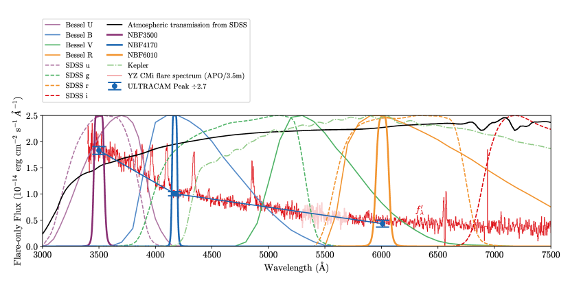
Figure 33: Quantum efficiency curves of common optical filters, normalized to peak transmission. An example of a terrestrial atmospheric transmission curve from the Sloan Digital Sky Survey is shown for an airmass of 1.0 at the Apache Point Observatory. One should note that the quantum efficiency of the CCD, telescope primary mirror, and other optical elements are not included. For reference, the impulsive phase flare spectrum from the IF4 event in [416] is shown. The wavelengths that are affected by the dichroic are in a lighter shade of red. The ULTRACAM photometry (NBF3500, NBF4170, NBF6010) at the peak of this flare were calibrated independently, and they are scaled to account for the factor of ten shorter integration time. The flare data were obtained from the Zenodo repository at: https://doi.org/10.5281/zenodo.45878.

In Fig. 33, we show the optical broadband and narrowband filters that are commonly used in stellar flare studies. There are numerous databases that provide these, such as the SVO Filter Profile Service at http://svo2.cab.inta-csic.es/theory/fps/, and some are published alongside photometry calibration surveys [67]. For comparison, we show the low-resolving power, flare-only spectrum [from Figure 3 of 416] over the impulsive phase of the IF event from the bottom panel of Fig. 8. The spectral shape from the calibrated ULTRACAM narrowband filters at the flare peak time is in agreement with the spectrum.

Appendix B A Summary of Supplemental Model Constraints in the Optical

In this appendix, we supplement the impulsive phase flare colors from spectra, shown in Fig. 12, with the peak colors calculated from narrow-band continuum filters. Fig. 34(top) is a summary of the peak-phase ULTRACAM filter (Appendix A) ratios from [416]. These flare colors were calculated at higher time resolution than from the spectra that were discussed in the main text (Sect. 7.2). Figure 34(middle) shows the evolution of the ULTRACAM filter ratios in the large IF1 event described in row (1a) of Table 7; see also Kowalski [409]. Average fluxes in the ULTRACAM narrowband filters are calculated from the spectra of the energetic IF3 event (also on YZ CMi) from [414] and are shown for comparison in Fig. 34(middle). Note, the peak flare spectrum for this event is showcased in Fig. 10. In the bottom panel, we show Balmer jump ratios against the ratios of the H$\gamma$ line flux to the flare-only continuum flux around $\lambda=4170$ Å at the time corresponding to the optical continuum peak flux. (The H$\gamma$ line flux is continuum-subtracted, integrated over the wavelengths of the line, and pre-flare subtracted; C4170^′ is the average the flare-only flux over $\lambda=4155-4185$ Å). Fig. 34(bottom) combines the impulsive-phase spectral measurements from [414] with the same quantities obtained in the four flares (indicated on the top axis) with low-resolving-power, optical spectra that were analyzed in [416] and [420]. It is our hope that as more flares are observed, these figures will be updated to provide compelling and comprehensive constraints for future multi-dimensional flare models.

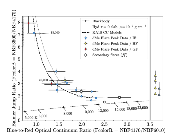
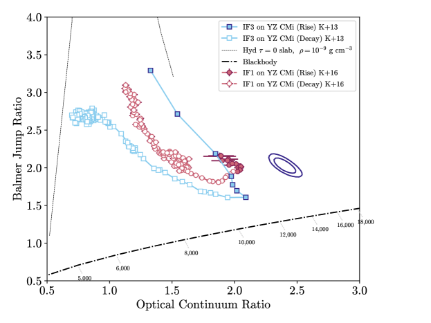
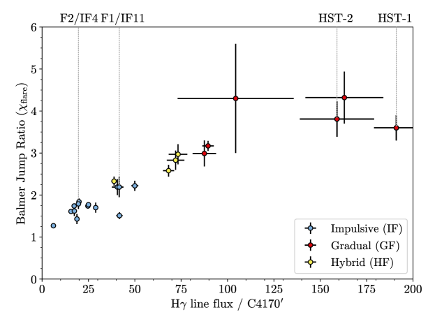
Figure 34: (Top) Flare-peak colors from ULTRACAM narrowband filter ratios; similar to Fig. 12 and see text for details. (Middle) Evolution of flare colors in two large flares on YZ CMi. Time increases over the tracks in a clockwise direction. These data have small statistical uncertainties (which are shown) but non-negligible systematic errors. The uncertainties are correlated, which we show for representative 5% systematic absolute color calibration uncertainties in both flare colors located at $(x,y)\approx(2,2)$. The error-ellipses indicate representative joint probabilities: the outer is the joint 68% confidence interval, while the inner translates to the marginal 68% uncertainties. (Bottom) Flare-only, line-to-continuum flux ratios from the same peak spectra in Fig. 12 in the main text.

Appendix C Slab Model Reference

C.1 Blackbody Fitting to Stellar Flare Optical Data

In this appendix, we summarize the assumptions and techniques employed by fitting isothermal blackbody functions to spectra, broadband photometry, and narrowband photometry of flares. A blackbody “color” temperature refers to the temperature of a blackbody that is fit to a ratio of two fluxes (e.g., a flare color calculated from a ratio of two flare-only continuum fluxes; Sect. 7.2.1), where color is equivalently a difference of magnitudes in two bandpasses. The term also refers to the temperature of a blackbody that is fit to the absolute value of more than two continuum flux values (outside of prominent emission lines) over a limited spectral range ($\Delta\lambda\approx 1000-2000$ Å). Generally, a color temperature contains rather limited information about the actual nature of the radiation, such as whether it is optically thick, thin, an intermediate optical thickness, or which atomic processes contribute to the emergent radiative flux. A color temperature does not unambiguously constrain how the spectrum of continuum radiation extends to wavelengths outside of the range over which it is calculated. Within the total wavelength span that a flare color is calculated (e.g., the ratio of flare fluxes in narrowband filters around 4170 Å and 6010 Å), there may be emission lines that affect the calculated value, and the actual spectrum between two wavelengths may be best represented by a more complex continuum model. Therefore, flare color temperatures are equivalent color temperatures of blackbody functions.

Other measures of temperature include gas temperature, radiation (or brightness) temperature, and effective temperature (in addition to the color temperatures of optically thin recombination and bremsstrahlung spectra). None of these are possible to robustly measure directly from optical stellar flare observations and must be inferred from detailed modeling. In principle, flare effective temperatures could be measured, but there has not yet been a more complete broadband spectral observation of a flare than analyzed in Hawley and Pettersen 297. To demonstrate the ambiguities in these measures of temperature, it is interesting to note that for an optically thin hydrogen recombination and free-free spectrum calculated from LTE level populations for a slab with a gas temperature of $T_{\rm{gas}}=10,000$ K (Appendix C.2, Fig. 37), the radiation temperature at $\lambda=4170$ Å is $T_{\rm{rad}}=3600$ K. The emergent intensities are calculated for a slab thickness of $dl=0.1$ km to ensure that $\tau(\lambda)<0.005$ across the optical regime. The color temperature measured from the ratio of intensities at $\lambda=4170$ Å to 6010 Å is $T_{\rm{FcolorR}}=5300$ K. Thus, $T_{\rm{gas}}>T_{\rm{FcolorR}}>T_{\rm{rad}}$ in this example.

Another interesting ambiguity in inferred gas temperatures occurs when the emergent continuum flux is formed over significant ($\tau\approx 1$) optical depth in dynamic, non-LTE, non-isothermal flare atmospheres. In Fig. 35, we summarize the argument in [409], which is also closely related to the analyses in the appendices of [418]. Two Planck functions with $T=13,000$ K and $T=14,000$ K are shown. If wavelength-dependent, continuum optical depths are large over an inhomogeneous temperature structure, then one could possibly, for example, measure radiation temperatures of $T_{\rm{rad}}=13,000$ K at $\lambda=4170$ Å and $T_{\rm{rad}}=14,000$ K at $\lambda=6010$ Å. The ratio of the corresponding emergent intensities gives a color temperature that is only $T_{\rm{FcolorR}}=10,500$ K. Thus, $T_{\rm{rad}}>T_{\rm{FcolorR}}$ in this example. For semi-infinite atmospheres that exhibit a linear dependence between the optical depth and the (LTE or non-LTE) source function, the Eddington-Barbier approximation relates the radiation temperature to the gas temperature at the depth corresponding to $\tau(\lambda)=1$; however, dynamic flare atmosphere calculations are usually much more complicated over the large physical depth ranges of continuum formation (e.g., in chromospheric condensations and the stationary layers below; cf. Fig. 2(right) and Fig. 21), which results in differences between the radiation temperature and the gas temperatures over which the emergent continuum intensity forms [see 409, for details].

Figure 35: Demonstration showing the relationship between a color temperature and wavelength-dependent radiation (brightness) temperatures at $\lambda=4170$ Å and $\lambda=6010$ Å.

The temperatures and filling factors calculated from optical and NUV flare data are in general obtained through two methods:

1. From a ratio of flare-only fluxes in two bandpasses, one can solve for the temperature and filling factor ($T_{\rm{flare}}$, $X_{\rm{flare}}$) of a Planck function following Hawley et al 298 (i.e., by equating ratios of the RHS of Eq. 28 in Sect. 12 to the observed flare-only ratio). The ratio equation is a transcendental equation for $T_{\rm{flare}}$ and can be solved numerically using linearization and iteration (i.e., Newton-Raphson) or through a simple lookup table. The result for $T_{\rm{flare}}$ is used to infer $X_{\rm{flare}}$.

   As discussed in [392] and [121], by not accounting for the fraction of stellar flux ($X_{\rm{flare}}$) that no longer shines through with the quiescent brightness, such as in a blackbody flare [see 298] or a flare with a transient overlying absorbing layer, it is possible to calculate a color temperature of $\approx 8500$ K from flare-only irradiance observations of solar flares, as reported in Kretzschmar [422]. In Fig. 36, we demonstrate what happens to the calculated color temperature of an optically thick ($\tau\gg 1$) flare source if one does not use the proper equation in [298]. For example, a 5800 K Planck function subtracted from a 7800 K Planck function at $\lambda_{1}=4170$ Å and $\lambda_{2}=6010$ Å gives a blackbody color temperature of 9000 K (c.f., where the 9000 K solid line and the 7500 K dashed line approximately intersect). However, for certain conditions, $S_{\lambda,\rm{flare}}\gg S_{\lambda,q}$ where $S_{\lambda,\rm{flare}}$ is the model flare surface flux spectrum, one may ignore the background subtraction errors (in which case, the problem must still be solved numerically or through a simple lookup table). Using the actual quiet Sun photospheric intensity, which is larger than a Planck function at these wavelengths, a 7500 K Planck function is sufficient to produce a 9000 K blackbody shape in the subtraction residuals. The surface fluxes of M dwarfs are much fainter than on G dwarfs. M-dwarf surface fluxes are lower than blackbody functions given by their effective temperatures, and the errors indicated in Fig. 36 are consequently smaller. For optically thick emission lines, similar issues arise if the model surface fluxes are comparable to the pre-flare surface fluxes (thus, it is fortuitous that large electron beam flux models produce spectra that are extremely bright compared to the pre-flare surface flux spectrum!).

   

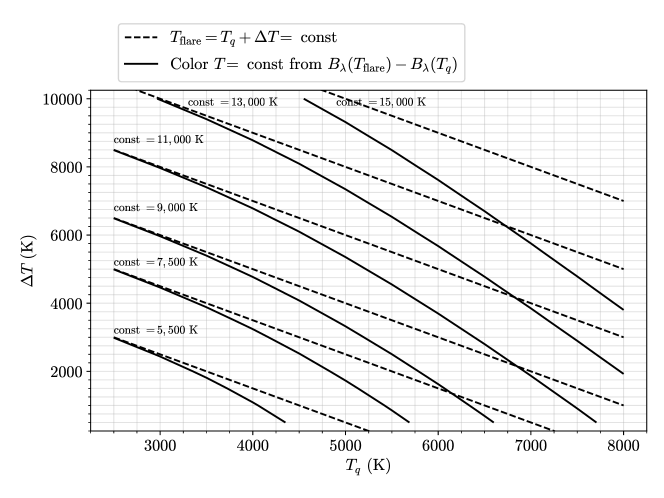
   Figure 36: Lines of constant blackbody flare temperatures ($T_{\rm{flare}}$) and lines of constant blackbody color temperatures that are calculated after subtracting a quiescent blackbody surface flux spectrum, $S_{\lambda,q}=B_{\lambda}(T_{q})$, from the flare model spectrum, $S_{\lambda,\mathrm{flare}}=B_{\lambda}(T_{\rm{flare}})$. The color temperature calculations, here shown for $\lambda_{1}=4170$ Å and $\lambda_{2}=6010$ Å, from stellar flare data usually account for or consider these issues in M dwarf flares [298, 416], but hotter flare color temperatures in higher-mass stars could be a result of “oversubtraction” effects.

2. Second, a color temperature can be fit to a spectrum of observed fluxes. A Planck function is typically fit to the excess (flare-only) spectrum, or to flare-only multi-band photometry data [302], with $n\lambda$ points ($n>2$) and Gaussian uncertainties, thus deriving the maximum likelihood parameters $\hat{T}_{\rm{flare}},\hat{X}_{\rm{flare}}$. This can be accomplished with non-linear least squares through linearization and iteration for unconstrained parameter fits and with the Levenberg-Marquardt algorithm (e.g., IDL’s mpcurvefit) for constrained parameter fits. The color temperatures (e.g., $T_{\rm{BB}}$) that were quoted from blackbody fitting in [414] were obtained by fitting Planck functions directly to the observed flare-only spectral fluxes (i.e., assuming $B_{\lambda}(T_{\rm{flare}})\gg S_{\lambda,q}$). Also in that paper, the excess RHD model flux spectra were similarly compared to a Planck function temperature without subtracting a pre-flare from the Planck function. In this approach, the color temperature is just a convenient parametrization for comparing models to flare-only spectral observations, since temperatures are easier to compare than color indices in different filters or at different wavelengths (as noted in the main text). Whatever one does to the data, one should also do analogously to the model, whether the model is a blackbody or an RHD spectrum, irrespective of spectral type of the star (from RHD models of M dwarf flares that are optically thin in the chromospheric continuum radiation, it is actually desirable to isolate the chromospheric flare radiation by subtracting the pre-flare surface flux because the model photospheric spectrum, which does not have proper molecular opacities, otherwise shines through and obfuscates comparisons to observations).

The main purpose of subtracting a pre-flare spectrum from the flare observations is to remove the relatively large, wavelength-dependent flux from the area on the star that is not flaring so that the flare emission is more accurately characterized. A method for determining an accurate subtraction of the preflare spectrum based on molecular bandpass veiling by the flare continuum is described in [414]. Alternatively, a very wide slit may be employed, but spectral purity and wavelength resolution are sacrificed; see [416].

In summary, the first method uses two filters and assumes that the flare spectrum is inherently blackbody radiation emitting at a single temperature $T_{\rm{flare}}$, and the second method is used for calculating color temperatures ($T_{\rm{BB}},T_{\rm{FcolorR}}$) directly from a spectrum of flare-only fluxes assuming that the effects in Figure 35 are not important (although this assumption can readily be relaxed in the second method).

C.2 Hydrogen Continuum Emissivity Models

[428] calculated a grid of optically thin, LTE hydrogen recombination models with free-free contributions. These are often used as a starting place for comparisons to flare observations (e.g., Fig. 12). The equations are not included in [428] but were restated in [406]. Here, we update the calculations with free-free Gaunt factors from CHIANTI and include the dissolved-level Balmer continuum components (longward of the Balmer edge at $\lambda=3646$ Å) in the spectra. These are shown in Fig. 37 for a range of temperatures and a gas density of $\rho=10^{-8}$ g cm^-3. The Balmer jump ratios are calculated from these spectra and are shown in Fig. 38. All spectra are available as FITS tables for a range of gas densities in the supplemental online material hosted on Zenodo.

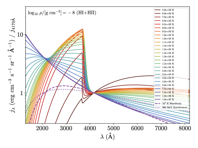
Figure 37: Hydrogen LTE emissivity calculations with bound-free (recombination) emissivity from H I and H^- and free-free (thermal bremsstrahlung) emissivity from H II. The spectral shapes here are identical to the shapes of intensity spectra, $I_{\lambda}$, that emerge from optically thin, homogeneous slabs. A blackbody function and a mono-energetic synchrotron spectrum is shown for comparison. The smooth transitions from the Balmer jump to the optical wavelengths are caused by the “dissolved level Balmer continuum” [154], which extends to redder wavelengths for larger electron densities.

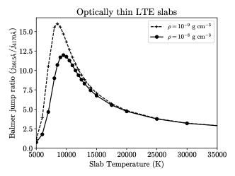
Figure 38: Balmer jump ratios calculated from the LTE emissivity models in Fig. 37 and from the same calculations of the LTE emissivity in a hydrogen gas with a density of $\rho=10^{-9}$ g cm^-3.

At constant slab temperature, a large range of flare colors result from adjusting the continuum optical depths [512]. In Fig. 39, we show the LTE continuum spectra from RHD model parameterizations [410]; the colors of these spectra are calculated and are shown in Fig. 12 as the “KA18 CC Models”. A range of reference column masses ($m_{\rm{ref}}$) were chosen to increase the continuum optical depths within the model chromospheric condensations. Occupational probabilities ($w_{n}$) for the dissolved level Balmer continuum opacities are included as in Figure 37.

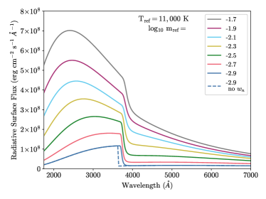
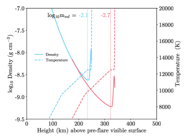
Figure 39: (Left) LTE continuum flux spectra calculated from the parameterized evolution of chromospheric condensations from RHD models. (Right) Examples of two of the parameterized atmospheres.

Appendix D Pressure Broadening of Hydrogen Lines in Flares

Electric fields split the degenerate energy levels of hydrogen atoms, Rydberg atoms, and hydrogen-like ions by an amount directly proportional to the field magnitude [$\propto E^{1}$; e.g., 137, 68, 247, 267], which is commonly known as the linear Stark, or Stark-Lo Surdo effect. The splitting increases for larger $n$, and $n=1$ experiences only second-order energy shifts, which are small. Within a partially ionized gas, the electric fields from ambient, thermal charges (electrons and protons) within a Debye radius broaden spectral lines. This explains the broad hydrogen absorption profiles in main sequence A stars and white dwarfs (combined with, of course, large optical depths in their photospheric layers).

The symmetric, atomic energy-level shifts that are linearly proportional to an external, uniform electric field $\mathcal{E}$ are described by the quantum numbers $nqm$, according to the following absolute value (in cgs units):

$$|\Delta E^{(1)}|=|\frac{3a_{0}e}{2Z}nq\mathcal{E}|$$ (29)

In Eq. 29, $n$ is the principal quantum number, $q$ is the difference of two parabolic quantum numbers, $k_{1}-k_{2}$, that satisfy $n=k_{1}+k_{2}+\mid m\mid+1$, $m=m_{l}$ is the magnetic quantum number, $a_{0}$ is the Bohr radius, $e$ is the electron charge, and $Z$ is the nuclear charge (where $Z=1$ for hydrogen).

Fig. 40 shows the splitting of the energy levels of hydrogen in a static electric field. The energy shifts were calculated using Equation 29 and the quadratic (second-order) and cubic (third-order) perturbation terms for hydrogen [137, 68, 186, 267]. The second-order and third-order terms create asymmetric splittings but are only important for hydrogen at very high electric field strengths. The maximum possible wavelength shift for an allowed Balmer transition ($n_{\rm{lower}}=2$) and $\Delta m\pm 1,0$ follows from Eq. 29 and is proportional to [733]:

$$\big{(}\frac{n_{j}^{2}}{n_{j}^{2}-4}\big{)}^{2}(n_{j}(n_{j}-1)+2)n_{e}^{2/3}$$ (30)

where $\big{(}\frac{n_{j}^{2}}{n_{j}^{2}-4}\big{)}^{2}$ is the appropriate conversion from $dE$ to $d\lambda$, and $n_{j}$ is the upper level of the Balmer transition. This formula, which goes as $n_{j}^{2}$ in the limit of large $n_{j}$, is sometimes used as an equivalent Doppler width that is added in quadrature with the true Doppler width in a Voigt profile. However, this approximation, among others [703], predicts inaccurate scalings for the line shapes and widths within a series. Thus, we recommend that these approximations not be used in place of proper line broadening calculations, which we briefly summarize next.

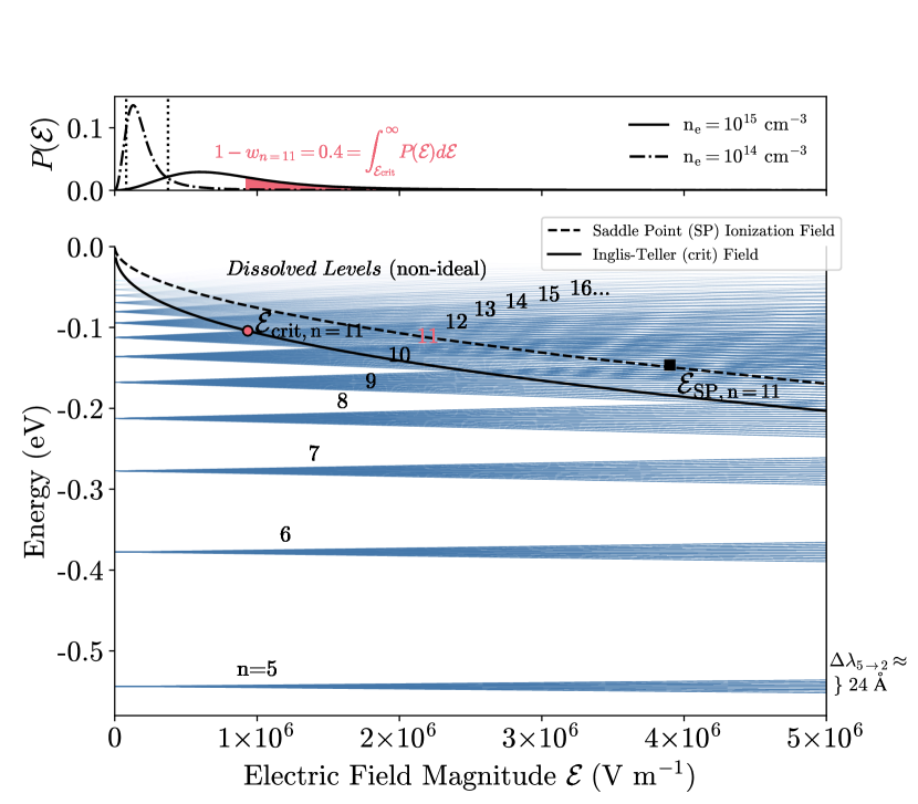
Figure 40: Energy level splitting for hydrogen in a static external electric field as a function of the electric field (in SI units). A principal level $n$ is split into roughly $2n-1$ (including the unshifted) sub-states. For even $n$, there is an unshifted component. Every split sub-state ($k_{1},k_{2},m$) is a mix of all the $l$-states for that value of $n$. The maximum splitting of the $n=5$ level shown here corresponds to 0.016 eV, which would correspond to a maximum wavelength displacement of $\Delta\lambda\approx 24$ Å for the H$\gamma$ transition. Only levels that can result in a dipole transition with $n=2$ have been plotted. The transitions with $\Delta m=0$ are known as the $\pi$ components, and $\Delta m\pm 1$ are the $\sigma$ components. The field strength that forms a “saddle point” (potential energy maximum) and destroys all levels $>n$ in hydrogen is shown as a function of $n$ [if there is a saddle-point in the potential, then tunneling is allowed as well; 68]. The field ionization of hydrogen has been observed (see the photograph from [606] that is reproduced in Montgomery et al 509). The Inglis-Teller relation corresponds to the critical field that causes the “bluest” sub-state of $n$ to intersect with the “reddest” sub-state of $n+1$, which occurs at a much smaller electric field for a given $n$ than the saddle point estimate (the ratio of the critical field to the saddle-point field is given by the factor known as $K_{n}$ in the literature). Holtsmark probability distributions of electric field magnitudes are shown in the top panel to illustrate an occupational probability ($w_{n}$) calculation for $n=11$ and $n_{e}=10^{15}$ cm^-3. A “normal field”, $F_{0}$, is the electric field magnitude at an average interparticle separation; the critical fields for $n_{e}=10^{14}$ and $10^{15}$ cm^-3 are indicated by vertical dotted lines in the top panel.

In a partially ionized gas, the electric microfield amplitude and direction vary from atom to atom and are not constant in time even at one atom because the charge distribution changes. The microfield amplitude probability is described by a probability distribution function (e.g., in the top panel of Fig. 40). A brief phenomenological summary of the microphysics of the broadening of hydrogen spectral lines follows. See [51], [262], [271], [337] for more comprehensive and rigorous reviews. The densities of perturbing, ambient (thermal) protons ($n_{p}$) and electrons ($n_{e}$) affect the total electric pressure broadening of radiative (dipole) transitions in hydrogen differently. The slow-moving protons and ions produce quasi-static [meaning that the microfield changes slowly compared to radiative/orbital timescales; see 275, 348] electric microfields that split the energy levels of hydrogen into sub-states (Fig. 40), which are superpositions of the various orbital angular momentum states, $l$, within each $n$ (“manifold”). The microfield magnitude is given by a Hooper probability distribution [which is a modified Holtsmark distribution that accounts for Debye screening and plasma correlations; 532]. The collisional perturbations from ambient electrons are more complicated. Classically, the individual elastic electron impacts on each atom are randomly occurring and well-separated in time, thus causing a damping/Lorentzian profile function with broadening FWHM $\Gamma$ that is proportional to $n_{e}$. However, on very short timescales, which correspond to large frequency displacements from line center (in the far line wings) in Fourier-conjugate space, the surrounding electrons are nearly still and thus produce a quasi-static (Holtsmark) broadening proportional to $n_{e}^{2/3}$. The transition in electron broadening from its impact to its quasistatic regimes occurs at wavelength shifts, of order $|\lambda-\lambda_{\rm{rest}}|\approx 20$ Å (for the H$\gamma$ line). Thus, large optical depths can make the effects of the quasi-static limit of electrons important in the wings. Additionally, lifetime broadening occurs if there are inelastic effects, such as collisional transitions to states of different principle quantum number $n$ [e.g., 348, 86], but these are generally small for well-separated levels (and are ignored in the “no-quenching” assumption in the VCS73 theory).

The energy-level perturbations from protons and from electron collisions are not independent random variables, and the line profiles thus cannot be modeled as convolutions of two probability distribution functions, such as a Lorentzian convolved with a Holtsmark (or Hooper) distribution. This is because the electron collisions with hydrogen are transient (short duration) and non-adiabatic [686, 689, 262, 337]: they can cause transitions and redistribution among the microfield-split sub-states of the same $n$. Quantum calculations [Eq 10 of 721, which is reproduced from Vidal et al 744] that account for the perturbing electrons in both of their limiting regimes are crucial. If the dynamical aspects [692] of the ions are ignored, the normalized line profile functions are then the ionic microfield averages of the electronic broadening profiles calculated at each value of the quasi-static (QS), ionic microfield $\mathcal{E_{\rm{QS}}}$. When the spacing between the upper levels $n_{j}$ becomes small and the broadening causes the states to have a significant probability of overlapping, level dissolution occurs and the bound-bound transitions become narrower [665, 721] and less Holtsmark-like in the wings. The extensions of the VCS73 profiles that account for the effects of level dissolution through occupational probabilities (Sect. 10.2.1) are known as the TB09$+$HM88 profiles. [130] discuss comparisons of high-density analytic profiles to new numerical calculations without level dissolution effects [see also 694, 269]. To our knowledge, the TB09$+$HM88 profiles are yet the only quantum calculations extended to large $n_{j}$ that also include a framework, albeit phenomenological, for ionization-limit lowering consistently with the bound-bound opacities and line shapes. This method is adequate for model spectra of the A0 V star Vega [e.g., 418], and thus by extension for flare models, given that there is an unfortunate paucity of echelle observations in this spectral region in stellar [241, 243] and solar [173] flares.

References

- \bibcommenthead
- Abbett [1998] Abbett WP (1998) A Theoretical Investigation of Optical Emission in Solar Flares. PhD thesis, Michigan State University
- Abbett and Hawley [1999] Abbett WP, Hawley SL (1999) Dynamic Models of Optical Emission in Impulsive Solar Flares. ApJ521:906–919. 10.1086/307576
- Aboudarham and Henoux [1986] Aboudarham J, Henoux JC (1986) Non-thermal excitation and ionization of hydrogen in solar flares. I. Effects on a flaring chromosphere. A&A168(1-2):301–307
- Adams et al [2011] Adams FC, Cai MJ, Galli D, et al (2011) Magnetic Interactions in Pre-main-sequence Binaries. ApJ743(2):175. 10.1088/0004-637X/743/2/175, arXiv:1110.4562 [astro-ph.SR]
- Agol et al [2021] Agol E, Dorn C, Grimm SL, et al (2021) Refining the Transit-timing and Photometric Analysis of TRAPPIST-1: Masses, Radii, Densities, Dynamics, and Ephemerides. Planet. Space Sci.2(1):1. 10.3847/PSJ/abd022, arXiv:2010.01074 [astro-ph.EP]
- Alaoui and Holman [2017] Alaoui M, Holman GD (2017) Understanding Breaks in Flare X-Ray Spectra: Evaluation of a Cospatial Collisional Return-current Model. ApJ851(2):78. 10.3847/1538-4357/aa98de, arXiv:1706.03897 [astro-ph.SR]
- Alaoui et al [2021] Alaoui M, Holman GD, Allred JC, et al (2021) Role of Suprathermal Runaway Electrons Returning to the Acceleration Region in Solar Flares. ApJ917(2):74. 10.3847/1538-4357/ac0820, arXiv:2103.13999 [astro-ph.SR]
- Allred et al [2005] Allred JC, Hawley SL, Abbett WP, et al (2005) Radiative Hydrodynamic Models of the Optical and Ultraviolet Emission from Solar Flares. ApJ630:573–586. 10.1086/431751, astro-ph/0507335
- Allred et al [2006] Allred JC, Hawley SL, Abbett WP, et al (2006) Radiative Hydrodynamic Models of Optical and Ultraviolet Emission from M Dwarf Flares. ApJ644:484–496. 10.1086/503314, astro-ph/0603195
- Allred et al [2015] Allred JC, Kowalski AF, Carlsson M (2015) A Unified Computational Model for Solar and Stellar Flares. ApJ809:104. 10.1088/0004-637X/809/1/104, arXiv:1507.04375 [astro-ph.SR]
- Allred et al [2020] Allred JC, Alaoui M, Kowalski AF, et al (2020) Modeling the Transport of Nonthermal Particles in Flares Using Fokker-Planck Kinetic Theory. ApJ902(1):16. 10.3847/1538-4357/abb239, arXiv:2008.10671 [astro-ph.SR]
- Allred et al [2022] Allred JC, Kerr GS, Gordon Emslie A (2022) Solar Flare Heating with Turbulent Suppression of Thermal Conduction. ApJ931(1):60. 10.3847/1538-4357/ac69e8, arXiv:2204.11684 [astro-ph.SR]
- Altyntsev et al [2019] Altyntsev AT, Meshalkina NS, Lysenko AL, et al (2019) Rapid Variability in the SOL2011-08-04 Flare: Implications for Electron Acceleration. ApJ883(1):38. 10.3847/1538-4357/ab3808, arXiv:1909.03593 [astro-ph.SR]
- Alvarado-Gómez et al [2018] Alvarado-Gómez JD, Drake JJ, Cohen O, et al (2018) Suppression of Coronal Mass Ejections in Active Stars by an Overlying Large-scale Magnetic Field: A Numerical Study. ApJ862(2):93. 10.3847/1538-4357/aacb7f, arXiv:1806.02828 [astro-ph.SR]
- Alvarado-Gómez et al [2020] Alvarado-Gómez JD, Drake JJ, Fraschetti F, et al (2020) Tuning the Exospace Weather Radio for Stellar Coronal Mass Ejections. ApJ895(1):47. 10.3847/1538-4357/ab88a3, arXiv:2004.05379 [astro-ph.SR]
- Anfinogentov et al [2013] Anfinogentov S, Nakariakov VM, Mathioudakis M, et al (2013) The Decaying Long-period Oscillation of a Stellar Megaflare. ApJ773(2):156. 10.1088/0004-637X/773/2/156
- Anglada-Escudé et al [2016] Anglada-Escudé G, Amado PJ, Barnes J, et al (2016) A terrestrial planet candidate in a temperate orbit around Proxima Centauri. Nature536(7617):437–440. 10.1038/nature19106, arXiv:1609.03449 [astro-ph.EP]
- Anstee and O’Mara [1995] Anstee SD, O’Mara BJ (1995) Width cross-sections for collisional broadening of s-p and p-s transitions by atomic hydrogen. MNRAS276(3):859–866. 10.1093/mnras/276.3.859
- Arber et al [2015] Arber TD, Bennett K, Brady CS, et al (2015) Contemporary particle-in-cell approach to laser-plasma modelling. Plasma Physics and Controlled Fusion 57(11):113001. 10.1088/0741-3335/57/11/113001
- Argiroffi et al [2019] Argiroffi C, Reale F, Drake JJ, et al (2019) A stellar flare-coronal mass ejection event revealed by X-ray plasma motions. Nature Astronomy 3:742–748. 10.1038/s41550-019-0781-4, arXiv:1905.11325 [astro-ph.SR]
- Arnold et al [2021] Arnold H, Drake JF, Swisdak M, et al (2021) Electron Acceleration during Macroscale Magnetic Reconnection. Phys. Rev. Lett.126(13):135101. 10.1103/PhysRevLett.126.135101, arXiv:2011.01147 [physics.plasm-ph]
- Aschwanden [1996] Aschwanden MJ (1996) Hard X-ray timing. In: Ramaty R, Mandzhavidze N, Hua XM (eds) High energy solar Physics, pp 300–310, 10.1063/1.50965
- Aschwanden [2004a] Aschwanden MJ (2004a) Physics of the Solar Corona. An Introduction
- Aschwanden [2004b] Aschwanden MJ (2004b) Pulsed Particle Injection in a Reconnection-Driven Dynamic Trap Model in Solar Flares. ApJ608(1):554–561. 10.1086/392494
- Aschwanden [2011] Aschwanden MJ (2011) Self-Organized Criticality in Astrophysics
- Aschwanden [2014] Aschwanden MJ (2014) A Macroscopic Description of a Generalized Self-organized Criticality System: Astrophysical Applications. ApJ782(1):54. 10.1088/0004-637X/782/1/54, arXiv:1310.4191 [astro-ph.SR]
- Aschwanden [2015] Aschwanden MJ (2015) Magnetic Energy Dissipation during the 2014 March 29 Solar Flare. ApJ804(1):L20. 10.1088/2041-8205/804/1/L20, arXiv:1504.03301 [astro-ph.SR]
- Aschwanden and Alexander [2001] Aschwanden MJ, Alexander D (2001) Flare Plasma Cooling from 30 MK down to 1 MK modeled from Yohkoh, GOES, and TRACE observations during the Bastille Day Event (14 July 2000). Sol. Phys.204:91–120. 10.1023/A:1014257826116
- Aschwanden and Freeland [2012] Aschwanden MJ, Freeland SL (2012) Automated Solar Flare Statistics in Soft X-Rays over 37 Years of GOES Observations: The Invariance of Self-organized Criticality during Three Solar Cycles. ApJ754(2):112. 10.1088/0004-637X/754/2/112, arXiv:1205.6712 [astro-ph.SR]
- Aschwanden and Güdel [2021] Aschwanden MJ, Güdel M (2021) Self-organized Criticality in Stellar Flares. ApJ910(1):41. 10.3847/1538-4357/abdec7, arXiv:2106.06490 [astro-ph.SR]
- Aschwanden et al [1995] Aschwanden MJ, Schwartz RA, Alt DM (1995) Electron Time-of-Flight Differences in Solar Flares. ApJ447:923. 10.1086/175930
- Aschwanden et al [1996a] Aschwanden MJ, Hudson H, Kosugi T, et al (1996a) Electron Time-of-Flight Measurements during the Masuda Flare, 1992 January 13. ApJ464:985. 10.1086/177386
- Aschwanden et al [1996b] Aschwanden MJ, Kosugi T, Hudson HS, et al (1996b) The Scaling Law between Electron Time-of-Flight Distances and Loop Lengths in Solar Flares. ApJ470:1198. 10.1086/177943
- Aschwanden et al [2008] Aschwanden MJ, Stern RA, Güdel M (2008) Scaling Laws of Solar and Stellar Flares. ApJ672(1):659–673. 10.1086/523926, arXiv:0710.2563 [astro-ph]
- Ashfield and Longcope [2023] Ashfield W, Longcope D (2023) A Model for Gradual-phase Heating Driven by MHD Turbulence in Solar Flares. ApJ944(2):147. 10.3847/1538-4357/acb1b2, arXiv:2301.04592 [astro-ph.SR]
- Astudillo-Defru et al [2017] Astudillo-Defru N, Delfosse X, Bonfils X, et al (2017) Magnetic activity in the HARPS M dwarf sample. The rotation-activity relationship for very low-mass stars through R’HK. A&A600:A13. 10.1051/0004-6361/201527078, arXiv:1610.09007 [astro-ph.SR]
- Atzeni and Meyer-ter Vehn [2004] Atzeni S, Meyer-ter Vehn J (2004) The Physics of Inertial Fusion: BeamPlasma Interaction, Hydrodynamics, Hot Dense Matter. Oxford University Press, 10.1093/acprof:oso/9780198562641.001.0001, URL https://doi.org/10.1093/acprof:oso/9780198562641.001.0001
- Audard et al [1999] Audard M, Güdel M, Guinan EF (1999) Implications from Extreme-Ultraviolet Observations for Coronal Heating of Active Stars. ApJ513(1):L53–L56. 10.1086/311907
- Audard et al [2000] Audard M, Güdel M, Drake JJ, et al (2000) Extreme-Ultraviolet Flare Activity in Late-Type Stars. ApJ541(1):396–409. 10.1086/309426, arXiv:astro-ph/0005062 [astro-ph]
- Audard et al [2007] Audard M, Briggs KR, Grosso N, et al (2007) The XMM-Newton Optical Monitor survey of the Taurus molecular cloud. A&A468(2):379–390. 10.1051/0004-6361:20066320, arXiv:astro-ph/0611367 [astro-ph]
- Aulanier et al [2013] Aulanier G, Démoulin P, Schrijver CJ, et al (2013) The standard flare model in three dimensions. II. Upper limit on solar flare energy. A&A549:A66. 10.1051/0004-6361/201220406, arXiv:1212.2086 [astro-ph.SR]
- Ayres [2015a] Ayres TR (2015a) The Far-Ultraviolet Ups and Downs of Alpha Centauri. AJ149(2):58. 10.1088/0004-6256/149/2/58
- Ayres [2015b] Ayres TR (2015b) The Flare-ona of EK Draconis. AJ150:7. 10.1088/0004-6256/150/1/7, arXiv:1505.02320 [astro-ph.SR]
- Ayres et al [1994] Ayres TR, Stauffer JR, Simon T, et al (1994) A Far-Ultraviolet Flare on a Pleiades G Dwarf. ApJ420:L33. 10.1086/187156
- Ayres et al [1998] Ayres TR, Simon T, Stern RA, et al (1998) The Coronae of Moderate-Mass Giants in the Hertzsprung Gap and the Clump. ApJ496(1):428–448. 10.1086/305347
- Ayres et al [1999] Ayres TR, Osten RA, Brown A (1999) The Rise and Fall of Velorum: A Remarkable Flare on a Yellow Giant Star Observed with the Extreme Ultraviolet Explorer. ApJ526(1):445–450. 10.1086/308001
- Ayres et al [2001] Ayres TR, Osten RA, Brown A (2001) 3 Ms in the Life of Ceti: Sustained Flare Activity on a Clump Giant Detected by the Extreme Ultraviolet Explorer. ApJ562(1):L83–L86. 10.1086/337971
- Balona [2012] Balona LA (2012) Kepler observations of flaring in A-F type stars. MNRAS423(4):3420–3429. 10.1111/j.1365-2966.2012.21135.x
- Balona [2019] Balona LA (2019) Evidence for spots on hot stars suggests major revision of stellar physics. MNRAS490(2):2112–2116. 10.1093/mnras/stz2808, arXiv:1910.01584 [astro-ph.SR]
- Balona et al [2015] Balona LA, Broomhall AM, Kosovichev A, et al (2015) Oscillations in stellar superflares. MNRAS450(1):956–966. 10.1093/mnras/stv661, arXiv:1504.01491 [astro-ph.SR]
- Barklem [2016] Barklem PS (2016) Accurate abundance analysis of late-type stars: advances in atomic physics. A&A Rev.24(1):9. 10.1007/s00159-016-0095-9, arXiv:1604.07659 [astro-ph.SR]
- Barklem and O’Mara [1998] Barklem PS, O’Mara BJ (1998) The broadening of strong lines of Ca+̂, Mg+̂ and Ba+̂ by collisions with neutral hydrogen atoms. MNRAS300(3):863–871. 10.1046/j.1365-8711.1998.01942.x
- Barklem et al [2000] Barklem PS, Piskunov N, O’Mara BJ (2000) Self-broadening in Balmer line wing formation in stellar atmospheres. A&A363:1091–1105. arXiv:astro-ph/0010022 [astro-ph]
- Baroch et al [2020] Baroch D, Morales JC, Ribas I, et al (2020) The CARMENES search for exoplanets around M dwarfs. Convective shift and starspot constraints from chromatic radial velocities. A&A641:A69. 10.1051/0004-6361/202038213, arXiv:2006.16608 [astro-ph.SR]
- Bastian [1990] Bastian TS (1990) Radio Emission from Flare Stars. Sol. Phys.130(1-2):265–294. 10.1007/BF00156794
- Bastian et al [1990] Bastian TS, Bookbinder J, Dulk GA, et al (1990) Dynamic Spectra of Radio Bursts from Flare Stars. ApJ353:265. 10.1086/168613
- Beasley and Bastian [1998] Beasley AJ, Bastian TS (1998) VLBA Imaging of UX Ari. In: Zensus JA, Taylor GB, Wrobel JM (eds) IAU Colloq. 164: Radio Emission from Galactic and Extragalactic Compact Sources, p 321
- Becker et al [2004] Becker AC, Wittman DM, Boeshaar PC, et al (2004) The Deep Lens Survey Transient Search. I. Short Timescale and Astrometric Variability. ApJ611(1):418–433. 10.1086/421994, arXiv:astro-ph/0404416 [astro-ph]
- Benenti et al [1999] Benenti G, Casati G, Shepelyansky DL (1999) Chaotic enhancement in microwave ionization of Rydberg atoms. European Physical Journal D 5(3):311–326. 10.1007/s100530050261, arXiv:cond-mat/9805216 [cond-mat]
- Benka and Holman [1992] Benka SG, Holman GD (1992) A Thermal/Nonthermal Model for Solar Microwave Bursts. ApJ391:854. 10.1086/171394
- Benz [2002] Benz A (2002) Plasma Astrophysics, second edition, vol 279. 10.1007/978-0-306-47719-5
- Benz [2017] Benz AO (2017) Flare Observations. Living Reviews in Solar Physics 14(1):2. 10.1007/s41116-016-0004-3
- Benz et al [1998] Benz AO, Conway J, Gudel M (1998) First VLBI images of a main-sequence star. A&A331:596–600
- Bergeman [1984] Bergeman T (1984) Relativistically enhanced ionization rates at Stark-effect level crossings in hydrogen. Phys. Rev. Lett.52(19):1685–1688. 10.1103/PhysRevLett.52.1685
- Berger et al [2013] Berger E, Leibler CN, Chornock R, et al (2013) A Search for Fast Optical Transients in the Pan-STARRS1 Medium-Deep Survey: M-Dwarf Flares, Asteroids, Limits on Extragalactic Rates, and Implications for LSST. ApJ779(1):18. 10.1088/0004-637X/779/1/18, arXiv:1307.5324 [astro-ph.HE]
- Beskin et al [2017] Beskin G, Karpov S, Plokhotnichenko V, et al (2017) Discovery of the Sub-second Linearly Polarized Spikes of Synchrotron Origin in the UV Ceti Giant Optical Flare. PASA34:e010. 10.1017/pasa.2017.3, arXiv:1702.06660 [astro-ph.SR]
- Bessell and Murphy [2012] Bessell M, Murphy S (2012) Spectrophotometric Libraries, Revised Photonic Passbands, and Zero Points for UBVRI, Hipparcos, and Tycho Photometry. PASP124:140. 10.1086/664083, arXiv:1112.2698 [astro-ph.SR]
- Bethe and Salpeter [1957] Bethe HA, Salpeter EE (1957) Quantum Mechanics of One- and Two-Electron Atoms
- Betta et al [1997] Betta R, Peres G, Reale F, et al (1997) An adaptive grid code for high resolution 1-D hydrodynamics of the solar and stellar transition region and corona. A&AS122:585–592. 10.1051/aas:1997157
- Bian et al [2012] Bian N, Emslie AG, Kontar EP (2012) A Classification Scheme for Turbulent Acceleration Processes in Solar Flares. ApJ754(2):103. 10.1088/0004-637X/754/2/103, arXiv:1206.0472 [astro-ph.SR]
- Bian et al [2018] Bian N, Emslie AG, Horne D, et al (2018) Heating and Cooling of Coronal Loops with Turbulent Suppression of Parallel Heat Conduction. ApJ852(2):127. 10.3847/1538-4357/aa9f29, arXiv:1711.11388 [astro-ph.SR]
- Bian et al [2014] Bian NH, Emslie AG, Stackhouse DJ, et al (2014) The Formation of Kappa-distribution Accelerated Electron Populations in Solar Flares. ApJ796(2):142. 10.1088/0004-637X/796/2/142, arXiv:1410.0819 [astro-ph.SR]
- Bice and Toomre [2020] Bice CP, Toomre J (2020) Probing the Influence of a Tachocline in Simulated M-dwarf Dynamos. ApJ893(2):107. 10.3847/1538-4357/ab8190, arXiv:2001.05555 [astro-ph.SR]
- Bice and Toomre [2022] Bice CP, Toomre J (2022) Longitudinally Modulated Dynamo Action in Simulated M-dwarf Stars. ApJ928(1):51. 10.3847/1538-4357/ac4be0, arXiv:2202.02869 [astro-ph.SR]
- Birn et al [2017] Birn J, Battaglia M, Fletcher L, et al (2017) Can Substorm Particle Acceleration Be Applied to Solar Flares? ApJ848(2):116. 10.3847/1538-4357/aa8ad4
- Bjørgen et al [2019] Bjørgen JP, Leenaarts J, Rempel M, et al (2019) Three-dimensional modeling of chromospheric spectral lines in a simulated active region. A&A631:A33. 10.1051/0004-6361/201834919, arXiv:1906.01098 [astro-ph.SR]
- Bookbinder et al [1992] Bookbinder JA, Walter FM, Brown A (1992) HST Observations of AD Leo. In: Giampapa MS, Bookbinder JA (eds) Cool Stars, Stellar Systems, and the Sun, p 27
- Bopp and Moffett [1973] Bopp BW, Moffett TJ (1973) High time resolution studies of UV Ceti. ApJ185:239. 10.1086/152412
- Bornmann [1987] Bornmann PL (1987) Turbulence as a Contributor to Intermediate Energy Storage during Solar Flares. ApJ313:449. 10.1086/164984
- Borucki et al [2010] Borucki WJ, Koch D, Basri G, et al (2010) Kepler Planet-Detection Mission: Introduction and First Results. Science 327(5968):977. 10.1126/science.1185402
- Boudreaux et al [2022] Boudreaux EM, Newton ER, Mondrik N, et al (2022) The Ca II H and K Rotation-Activity Relation in 53 Mid-to-late-type M Dwarfs. ApJ929(1):80. 10.3847/1538-4357/ac5cbf, arXiv:2203.04999 [astro-ph.SR]
- Bower et al [2003] Bower GC, Plambeck RL, Bolatto A, et al (2003) A Giant Outburst at Millimeter Wavelengths in the Orion Nebula. ApJ598(2):1140–1150. 10.1086/379101, arXiv:astro-ph/0308277 [astro-ph]
- Boyd and Sanderson [2003] Boyd TJM, Sanderson JJ (2003) The Physics of Plasmas
- Brandenburg [2005] Brandenburg A (2005) The Case for a Distributed Solar Dynamo Shaped by Near-Surface Shear. ApJ625(1):539–547. 10.1086/429584, arXiv:astro-ph/0502275 [astro-ph]
- Brandenburg and Subramanian [2005] Brandenburg A, Subramanian K (2005) Astrophysical magnetic fields and nonlinear dynamo theory. Phys. Rep.417(1-4):1–209. 10.1016/j.physrep.2005.06.005, arXiv:astro-ph/0405052 [astro-ph]
- Bransden and Joachain [2000] Bransden BH, Joachain CJ (2000) Quantum Mechanics. Pearson, Prentice Hall, Harlow, England :
- Brasseur et al [2019] Brasseur CE, Osten RA, Fleming SW (2019) Short-duration Stellar Flares in GALEX Data. ApJ883(1):88. 10.3847/1538-4357/ab3df8, arXiv:1908.08377 [astro-ph.SR]
- Brasseur et al [2023] Brasseur CE, Osten RA, Tristan II, et al (2023) Constraints on Stellar Flare Energy Ratios in the NUV and Optical from a Multiwavelength Study of GALEX and Kepler Flare Stars. ApJ944(1):5. 10.3847/1538-4357/acab59, arXiv:2212.08696 [astro-ph.SR]
- Bressan et al [2012] Bressan A, Marigo P, Girardi L, et al (2012) PARSEC: stellar tracks and isochrones with the PAdova and TRieste Stellar Evolution Code. MNRAS427(1):127–145. 10.1111/j.1365-2966.2012.21948.x, arXiv:1208.4498 [astro-ph.SR]
- Bromage et al [1986] Bromage GE, Phillips KJH, Dufton PL, et al (1986) Flares on dMe stars : IUE and optical observations of AT MIC and comparison of far-ultraviolet stellar and solar flares. MNRAS220:1021–1046. 10.1093/mnras/220.4.1021
- Broomhall et al [2019a] Broomhall AM, Davenport JRA, Hayes LA, et al (2019a) A Blueprint of State-of-the-art Techniques for Detecting Quasi-periodic Pulsations in Solar and Stellar Flares. ApJS244(2):44. 10.3847/1538-4365/ab40b3, arXiv:1910.08458 [astro-ph.SR]
- Broomhall et al [2019b] Broomhall AM, Thomas AEL, Pugh CE, et al (2019b) Multi-waveband detection of quasi-periodic pulsations in a stellar flare on EK Draconis observed by XMM-Newton. A&A629:A147. 10.1051/0004-6361/201935653, arXiv:1908.06033 [astro-ph.SR]
- Brosius and Inglis [2018] Brosius JW, Inglis AR (2018) Localized Quasi-periodic Fluctuations in C II, Si IV, and Fe XXI Emission during Chromospheric Evaporation in a Flare Ribbon Observed by IRIS on 2017 September 9. ApJ867(2):85. 10.3847/1538-4357/aae5f5
- Brown et al [2023] Brown A, Schneider PC, France K, et al (2023) Coronal X-Ray Emission from Nearby, Low-mass, Exoplanet Host Stars Observed by the MUSCLES and Mega-MUSCLES HST Treasury Survey Projects. AJ165(5):195. 10.3847/1538-3881/acc38a, arXiv:2303.12929 [astro-ph.SR]
- Brown et al [2020] Brown BP, Oishi JS, Vasil GM, et al (2020) Single-hemisphere Dynamos in M-dwarf Stars. ApJ902(1):L3. 10.3847/2041-8213/abb9a4, arXiv:2008.02362 [astro-ph.SR]
- Brown [1971] Brown JC (1971) The Deduction of Energy Spectra of Non-Thermal Electrons in Flares from the Observed Dynamic Spectra of Hard X-Ray Bursts. Sol. Phys.18(3):489–502. 10.1007/BF00149070
- Brown [1973] Brown JC (1973) The Temperature Structure of Chromospheric Flares Heated by Non-Thermal Electrons. Sol. Phys.31(1):143–169. 10.1007/BF00156080
- Brown et al [1998] Brown JC, Conway AJ, Aschwanden MJ (1998) The Electron Injection Function and Energy-dependent Delays in Thick-Target Hard X-Rays. ApJ509(2):911–917. 10.1086/306522
- Brown et al [2003] Brown JC, Emslie AG, Kontar EP (2003) The Determination and Use of Mean Electron Flux Spectra in Solar Flares. ApJ595(2):L115–L117. 10.1086/378169
- Brown and Brown [2006] Brown JM, Brown A (2006) A Large Millimeter Flare on the RS CVn Binary Geminorum. ApJ638(1):L37–L40. 10.1086/500929
- Browning [2008] Browning MK (2008) Simulations of Dynamo Action in Fully Convective Stars. ApJ676(2):1262–1280. 10.1086/527432, arXiv:0712.1603 [astro-ph]
- Brun and Browning [2017] Brun AS, Browning MK (2017) Magnetism, dynamo action and the solar-stellar connection. Living Reviews in Solar Physics 14(1):4. 10.1007/s41116-017-0007-8
- Butler et al [1981] Butler CJ, Byrne PB, Andrews AD, et al (1981) Ultraviolet spectra of dwarf solar neighbourhood stars. I. MNRAS197:815–827. 10.1093/mnras/197.3.815
- Butler et al [1988] Butler CJ, Rodono M, Foing BH (1988) A correlation between Balmer and soft X-ray emission from stellar andsolar flares. A&A206:L1–L4
- Butler et al [2015] Butler CJ, Erkan N, Budding E, et al (2015) A multiwavelength study of the M dwarf binary YY Geminorum. MNRAS446(4):4205–4219. 10.1093/mnras/stu2398, arXiv:1501.03930 [astro-ph.SR]
- Byrne [1989] Byrne PB (1989) Multi-Wavelength Observations of Stellar Flares. Sol. Phys.121(1-2):61–74. 10.1007/BF00161687
- Byrne et al [1990] Byrne PB, Butler CJ, Lyons MA (1990) Activity in late-type stars. VI. Optical photometry and UV spectroscopy of the active dMe star, FK Aquarii in late 1983. A&A236:455
- Caballero-García et al [2015] Caballero-García MD, Šimon V, Jelínek M, et al (2015) Early optical follow-up of the nearby active star DG CVn during its 2014 superflare. MNRAS452(4):4195–4202. 10.1093/mnras/stv1565, arXiv:1507.03143 [astro-ph.HE]
- Candelaresi et al [2014] Candelaresi S, Hillier A, Maehara H, et al (2014) Superflare Occurrence and Energies on G-, K-, and M-type Dwarfs. ApJ792(1):67. 10.1088/0004-637X/792/1/67, arXiv:1405.1453 [astro-ph.SR]
- Canfield et al [1990] Canfield RC, Penn MJ, Wulser JP, et al (1990) H alpha Spectra of Dynamic Chromospheric Processes in Five Well-observed X-Ray Flares. ApJ363:318. 10.1086/169345
- Canfield et al [1991] Canfield RC, Wulser JP, Zarro DM, et al (1991) A Study of Solar Flare Energy Transport Based on Coordinated H alpha and X-Ray Observations. ApJ367:671. 10.1086/169663
- Carlsson [1998] Carlsson M (1998) Radiative Transfer and Radiation Hydrodynamics. In: Vial JC, Bocchialini K, Boumier P (eds) Space Solar Physics: Theoretical and Observational Issues in the Context of the SOHO Mission, vol 507. p 163, 10.1007/BFb0106920
- Carlsson and Stein [1992] Carlsson M, Stein RF (1992) Non-LTE Radiating Acoustic Shocks and CA II K2V Bright Points. ApJ397:L59. 10.1086/186544
- Carlsson and Stein [1995] Carlsson M, Stein RF (1995) Does a Nonmagnetic Solar Chromosphere Exist? ApJ440:L29. 10.1086/187753, arXiv:astro-ph/9411036 [astro-ph]
- Carlsson and Stein [1997] Carlsson M, Stein RF (1997) Formation of Solar Calcium H and K Bright Grains. ApJ481:500–514
- Carlsson et al [2016] Carlsson M, Hansteen VH, Gudiksen BV, et al (2016) A publicly available simulation of an enhanced network region of the Sun. A&A585:A4. 10.1051/0004-6361/201527226, arXiv:1510.07581 [astro-ph.SR]
- Carlsson et al [2023] Carlsson M, Fletcher L, Allred J, et al (2023) The F-CHROMA grid of 1D RADYN flare models. A&A673:A150. 10.1051/0004-6361/202346087, arXiv:2304.02618 [astro-ph.SR]
- Carmichael [1964] Carmichael H (1964) A Process for Flares. In: NASA Special Publication, vol 50. p 451
- Cassak et al [2008] Cassak PA, Mullan DJ, Shay MA (2008) From Solar and Stellar Flares to Coronal Heating: Theory and Observations of How Magnetic Reconnection Regulates Coronal Conditions. ApJ676(1):L69. 10.1086/587055, arXiv:0710.3399 [astro-ph]
- Cassak et al [2017] Cassak PA, Liu YH, Shay MA (2017) A review of the 0.1 reconnection rate problem. Journal of Plasma Physics 83(5):715830501. 10.1017/S0022377817000666, arXiv:1708.03449 [physics.plasm-ph]
- Castellanos Durán and Kleint [2020] Castellanos Durán JS, Kleint L (2020) The Statistical Relationship between White-light Emission and Photospheric Magnetic Field Changes in Flares. ApJ904(2):96. 10.3847/1538-4357/ab9c1e
- Chambe and Henoux [1979] Chambe G, Henoux JC (1979) Direct excitation of hydrogen by photoelectron and accelerated electron collisions in solar chromospheric flares - Effects on the profile and polarization of LY alpha. A&A80(2):123–129
- Chandrasekhar [1960] Chandrasekhar S (1960) Radiative transfer
- Chang et al [2020] Chang SW, Wolf C, Onken CA (2020) Photometric flaring fraction of M dwarf stars from the SkyMapper Southern Survey. MNRAS491(1):39–50. 10.1093/mnras/stz2898, arXiv:1910.06478 [astro-ph.SR]
- Charbonneau [2013] Charbonneau P (2013) Solar and Stellar Dynamos, Saas-Fee Advanced Course, vol 39. 10.1007/978-3-642-32093-4
- Chen et al [2020] Chen B, Shen C, Gary DE, et al (2020) Measurement of magnetic field and relativistic electrons along a solar flare current sheet. Nature Astronomy 4:1140–1147. 10.1038/s41550-020-1147-7, arXiv:2005.12757 [astro-ph.SR]
- Cheng et al [2012] Cheng JX, Qiu J, Ding MD, et al (2012) Solar flare hard X-ray spikes observed by RHESSI: a statistical study. A&A547:A73. 10.1051/0004-6361/201118608, arXiv:1210.7027 [astro-ph.SR]
- Chintzoglou et al [2019] Chintzoglou G, Zhang J, Cheung MCM, et al (2019) The Origin of Major Solar Activity: Collisional Shearing between Nonconjugated Polarities of Multiple Bipoles Emerging within Active Regions. ApJ871(1):67. 10.3847/1538-4357/aaef30, arXiv:1811.02186 [astro-ph.SR]
- Cho et al [2016] Cho IH, Cho KS, Nakariakov VM, et al (2016) Comparison of Damped Oscillations in Solar and Stellar X-Ray flares. ApJ830(2):110. 10.3847/0004-637X/830/2/110
- Cho et al [2022] Cho PB, Gomez TA, Montgomery MH, et al (2022) Simulation of Stark-broadened Hydrogen Balmer-line Shapes for DA White Dwarf Synthetic Spectra. ApJ927(1):70. 10.3847/1538-4357/ac4df3
- Christian et al [2003] Christian DJ, Mathioudakis M, Jevremović D, et al (2003) The Extreme-Ultraviolet Continuum of a Strong Stellar Flare. ApJ593:L105–L108. 10.1086/378217
- Clarke et al [2018] Clarke RW, Davenport JRA, Covey KR, et al (2018) Flare Activity of Wide Binary Stars with Kepler. ApJ853(1):59. 10.3847/1538-4357/aaa0d3
- Clauset et al [2009] Clauset A, Shalizi CR, Newman MEJ (2009) Power-Law Distributions in Empirical Data. SIAM Review 51(4):661–703. 10.1137/070710111
- Cliver et al [1986] Cliver EW, Dennis BR, Kiplinger AL, et al (1986) Solar Gradual Hard X-Ray Bursts and Associated Phenomena. ApJ305:920. 10.1086/164306
- Cliver et al [2022a] Cliver EW, Pötzi W, Veronig AM (2022a) Large Sunspot Groups and Great Magnetic Storms: Magnetic Suppression of CMEs. ApJ938(2):136. 10.3847/1538-4357/ac847d
- Cliver et al [2022b] Cliver EW, Schrijver CJ, Shibata K, et al (2022b) Extreme solar events. Living Reviews in Solar Physics 19(1):2. 10.1007/s41116-022-00033-8, arXiv:2205.09265 [astro-ph.SR]
- Condon and Shortley [1963] Condon EU, Shortley GH (1963) The theory of atomic spectra
- Covey et al [2007] Covey KR, Ivezić Ž, Schlegel D, et al (2007) Stellar SEDs from 0.3 to 2.5 m: Tracing the Stellar Locus and Searching for Color Outliers in the SDSS and 2MASS. AJ134(6):2398–2417. 10.1086/522052
- Cox and Tucker [1969] Cox DP, Tucker WH (1969) Ionization Equilibrium and Radiative Cooling of a Low-Density Plasma. ApJ157:1157. 10.1086/150144
- Cram and Woods [1982] Cram LE, Woods DT (1982) Models for stellar flares. ApJ257:269–275. 10.1086/159985
- Cranmer [2021] Cranmer SR (2021) Brown Dwarfs are Violet: A New Calculation of Human-eye Colors of Main-sequence Stars and Substellar Objects. Research Notes of the American Astronomical Society 5(9):201. 10.3847/2515-5172/ac225c
- Crespo-Chacón et al [2004] Crespo-Chacón I, Montes D, Fernández-Figueroa MJ, et al (2004) High Temporal Resolution Spectroscopic Observations of the Flare Star V1054 Oph. Ap&SS292(1):697–703. 10.1023/B:ASTR.0000045077.58363.e4
- Crosby et al [1993] Crosby NB, Aschwanden MJ, Dennis BR (1993) Frequency distributions and correlations of solar X-ray flare parameters. Sol. Phys.143(2):275–299. 10.1007/BF00646488
- Crosley and Osten [2018] Crosley MK, Osten RA (2018) Constraining Stellar Coronal Mass Ejections through Multi-wavelength Analysis of the Active M Dwarf EQ Peg. ApJ856(1):39. 10.3847/1538-4357/aaaec2, arXiv:1802.03440 [astro-ph.SR]
- Cully et al [1994] Cully SL, Fisher GH, Abbott MJ, et al (1994) A coronal mass ejection model for the 1992 July 15 flare on AU Microscopii observed by the extreme ultraviolet explorer. ApJ435:449–463. 10.1086/174827
- Dahlin [2020] Dahlin JT (2020) Prospectus on electron acceleration via magnetic reconnection. Physics of Plasmas 27(10):100601. 10.1063/5.0019338
- Dahlin et al [2014] Dahlin JT, Drake JF, Swisdak M (2014) The mechanisms of electron heating and acceleration during magnetic reconnection. Physics of Plasmas 21(9):092304. 10.1063/1.4894484, arXiv:1406.0831 [physics.plasm-ph]
- Dahlin et al [2015] Dahlin JT, Drake JF, Swisdak M (2015) Electron acceleration in three-dimensional magnetic reconnection with a guide field. Physics of Plasmas 22(10):100704. 10.1063/1.4933212, arXiv:1503.02218 [physics.plasm-ph]
- Dal [2020] Dal HA (2020) The flare cumulative frequencies of UV Ceti stars from different spectral types. MNRAS495(4):4529–4541. 10.1093/mnras/staa1484
- Dal and Evren [2010] Dal HA, Evren S (2010) A New Method for Classifying Flares of UV Ceti Type Stars: Differences Between Slow and Fast Flares. AJ140(2):483–489. 10.1088/0004-6256/140/2/483, arXiv:1206.5791 [astro-ph.SR]
- Dal and Evren [2011a] Dal HA, Evren S (2011a) Rotation Modulations and Distributions of the Flare Occurrence Rates on the Surface of Five UV Ceti Type Stars. PASJ63:427–447. 10.1093/pasj/63.2.427, arXiv:1206.5792 [astro-ph.SR]
- Dal and Evren [2011b] Dal HA, Evren S (2011b) Saturation Levels for White-light Flares of Flare Stars: Variation of Minimum Flare Duration for Saturation. AJ141(2):33. 10.1088/0004-6256/141/2/33, arXiv:1206.5793 [astro-ph.SR]
- Damburg and Kolosov [1979] Damburg RJ, Kolosov VV (1979) A hydrogen atom in a uniform electric field. III. Journal of Physics B Atomic Molecular Physics 12(16):2637–2643. 10.1088/0022-3700/12/16/011
- Dappen et al [1987] Dappen W, Anderson L, Mihalas D (1987) Statistical mechanics of partially ionized stellar plasma - The Planck-Larkin partition function, polarization shifts, and simulations of optical spectra. ApJ319:195–206. 10.1086/165446
- Davenport [2016] Davenport JRA (2016) The Kepler Catalog of Stellar Flares. ApJ829:23. 10.3847/0004-637X/829/1/23, arXiv:1607.03494 [astro-ph.SR]
- Davenport et al [2012] Davenport JRA, Becker AC, Kowalski AF, et al (2012) Multi-wavelength Characterization of Stellar Flares on Low-mass Stars Using SDSS and 2MASS Time-domain Surveys. ApJ748(1):58. 10.1088/0004-637X/748/1/58
- Davenport et al [2014] Davenport JRA, Hawley SL, Hebb L, et al (2014) Kepler Flares. II. The Temporal Morphology of White-light Flares on GJ 1243. ApJ797:122. 10.1088/0004-637X/797/2/122, arXiv:1411.3723 [astro-ph.SR]
- Davenport et al [2015] Davenport JRA, Hebb L, Hawley SL (2015) Detecting Differential Rotation and Starspot Evolution on the M Dwarf GJ 1243 with Kepler. ApJ806(2):212. 10.1088/0004-637X/806/2/212, arXiv:1505.01524 [astro-ph.SR]
- Davenport et al [2016] Davenport JRA, Kipping DM, Sasselov D, et al (2016) MOST Observations of Our Nearest Neighbor: Flares on Proxima Centauri. ApJ829(2):L31. 10.3847/2041-8205/829/2/L31, arXiv:1608.06672 [astro-ph.SR]
- Davenport et al [2019] Davenport JRA, Covey KR, Clarke RW, et al (2019) The Evolution of Flare Activity with Stellar Age. ApJ871(2):241. 10.3847/1538-4357/aafb76
- Davenport et al [2020] Davenport JRA, Mendoza GT, Hawley SL (2020) 10 Years of Stellar Activity for GJ 1243. AJ160(1):36. 10.3847/1538-3881/ab9536, arXiv:2005.10281 [astro-ph.SR]
- Davison et al [2015] Davison CL, White RJ, Henry TJ, et al (2015) A 3D Search for Companions to 12 Nearby M Dwarfs. AJ149(3):106. 10.1088/0004-6256/149/3/106
- De Luca et al [2020] De Luca A, Stelzer B, Burgasser AJ, et al (2020) EXTraS discovery of an X-ray superflare from an L dwarf. A&A634:L13. 10.1051/0004-6361/201937163, arXiv:2002.08078 [astro-ph.SR]
- De Pontieu et al [2014] De Pontieu B, Title AM, Lemen JR, et al (2014) The Interface Region Imaging Spectrograph (IRIS). Sol. Phys.289:2733–2779. 10.1007/s11207-014-0485-y, arXiv:1401.2491 [astro-ph.SR]
- Dennis and Zarro [1993] Dennis BR, Zarro DM (1993) The Neupert effect - What can it tell us about the impulsive and gradual phases of solar flares? Sol. Phys.146:177–190. 10.1007/BF00662178
- Dennis et al [2011] Dennis BR, Emslie AG, Hudson HS (2011) Overview of the Volume. Space Sci. Rev.159(1-4):3–17. 10.1007/s11214-011-9802-z, arXiv:1109.5831 [astro-ph.SR]
- Dennis et al [2022] Dennis BR, Shih AY, Hurford GJ, et al (2022) Ramaty High Energy Solar Spectroscopic Imager (RHESSI). arXiv e-prints arXiv:2206.00741. arXiv:2206.00741 [astro-ph.SR]
- Dere et al [1997] Dere KP, Landi E, Mason HE, et al (1997) CHIANTI - an atomic database for emission lines. A&AS125:149–173. 10.1051/aas:1997368
- Dhillon et al [2007] Dhillon VS, Marsh TR, Stevenson MJ, et al (2007) ULTRACAM: an ultrafast, triple-beam CCD camera for high-speed astrophysics. MNRAS378(3):825–840. 10.1111/j.1365-2966.2007.11881.x
- Dimitrijević and Sahal-Bréchot [1992] Dimitrijević MS, Sahal-Bréchot S (1992) Stark broadening parameter tables for Ca II lines of astrophysical interest. Bulletin Astronomique de Belgrade 145:83–99
- Dimitrijevic and Sahal-Brechot [1993] Dimitrijevic MS, Sahal-Brechot S (1993) Stark broadening of Ca II spectral lines. J. Quant. Spec. Radiat. Transf.49(2):157–164. 10.1016/0022-4073(93)90056-N
- Donati et al [1997] Donati JF, Semel M, Carter BD, et al (1997) Spectropolarimetric observations of active stars. MNRAS291(4):658–682. 10.1093/mnras/291.4.658
- Donati-Falchi et al [1985] Donati-Falchi A, Falciani R, Smaldone LA (1985) Analysis of the optical spectra of solar flares. IV - The ’blue’ continuum of white light flares. A&A152:165–169
- Dorfi [1998] Dorfi EA (1998) Radiation Hydrodynamics: Numerical Aspects and Applications. In: Steiner O, Gautschy A (eds) Saas-Fee Advanced Course 27: Computational Methods for Astrophysical Fluid Flow., p 263
- Dorfi and Drury [1987] Dorfi EA, Drury LO (1987) Simple adaptive grids for 1-D initial value problems. Journal of Computational Physics 69:175–195. 10.1016/0021-9991(87)90161-6
- Doyle and Mathioudakis [1990] Doyle JG, Mathioudakis M (1990) Flare activity and orbital rotation of YY Geminorum. A&A227:130–132
- Doyle et al [1988a] Doyle JG, Butler CJ, Bryne PB, et al (1988a) Rotational modulation and flares on RS CVn and BY DRA systems. A&A193:229–247
- Doyle et al [1988b] Doyle JG, Butler CJ, Callanan PJ, et al (1988b) Rotational modulation and flares on RS CVn and BY DRA systems. VIII. Simultaneous EXOSAT and H alpha observations of a flare on the dMe star GL 644 AB (Wolf 630) on 24/25 August 1985. A&A191:79–86
- Doyle et al [1989] Doyle JG, van den Oord GHJ, Butler CJ (1989) Optical flares from the dwarf M star V577 MON (Gliese 234 AB = Ross 614). A&A208:208–212
- Doyle et al [1990a] Doyle JG, Butler CJ, van den Oord GHJ, et al (1990a) A periodicity in the flaring rate on the eclipsing binary YY Geminorum. A&A232:83
- Doyle et al [1990b] Doyle JG, Butler CJ, van den Oord GHJ, et al (1990b) A periodicity in the flaring rate on the eclipsing binary YY Geminorum. A&A232:83
- Doyle et al [2012] Doyle JG, Giunta A, Singh A, et al (2012) The Diagnostic Potential of Transition Region Lines Undergoing Transient Ionization in Dynamic Events. Sol. Phys.280(1):111–124. 10.1007/s11207-012-0025-6, arXiv:1204.6598 [astro-ph.SR]
- Doyle et al [2013] Doyle JG, Giunta A, Madjarska MS, et al (2013) Diagnosing transient ionization in dynamic events. A&A557:L9. 10.1051/0004-6361/201321902, arXiv:1307.8251 [astro-ph.SR]
- Doyle et al [2022] Doyle JG, Irawati P, Kolotkov DY, et al (2022) Doubling of minute-long quasi-periodic pulsations from super-flares on a low-mass star. MNRAS514(4):5178–5182. 10.1093/mnras/stac1695, arXiv:2206.08070 [astro-ph.SR]
- Doyle et al [2018] Doyle L, Ramsay G, Doyle JG, et al (2018) Investigating the rotational phase of stellar flares on M dwarfs using K2 short cadence data. MNRAS480(2):2153–2164. 10.1093/mnras/sty1963, arXiv:1807.08592 [astro-ph.SR]
- Drake [2006] Drake GWF (2006) Springer Handbook of Atomic, Molecular, and Optical Physics. 10.1007/978-0-387-26308-3
- Drake et al [2006] Drake JF, Swisdak M, Che H, et al (2006) Electron acceleration from contracting magnetic islands during reconnection. Nature443(7111):553–556. 10.1038/nature05116
- Drake et al [2013] Drake JF, Swisdak M, Fermo R (2013) The Power-law Spectra of Energetic Particles during Multi-island Magnetic Reconnection. ApJ763(1):L5. 10.1088/2041-8205/763/1/L5, arXiv:1210.4830 [astro-ph.SR]
- Drake et al [2019] Drake JF, Arnold H, Swisdak M, et al (2019) A computational model for exploring particle acceleration during reconnection in macroscale systems. Physics of Plasmas 26(1):012901. 10.1063/1.5058140, arXiv:1809.04568 [astro-ph.SR]
- Drake [2003] Drake JJ (2003) From the Heart of the Ghoul: C and N Abundances in the Corona of Algol B. ApJ594(1):496–509. 10.1086/375837, arXiv:astro-ph/0308230 [astro-ph]
- Drake and Ercolano [2007] Drake JJ, Ercolano B (2007) The Detectability of Neon Fluorescence and Measurement of the Solar Photospheric Neon Abundance. ApJ665(2):L175–L178. 10.1086/521190, arXiv:0708.1022 [astro-ph]
- Drake et al [2008] Drake JJ, Ercolano B, Swartz DA (2008) X-Ray-fluorescent Fe K Lines from Stellar Photospheres. ApJ678(1):385–393. 10.1086/524976, arXiv:0710.0621 [astro-ph]
- Drake and Ulrich [1980] Drake SA, Ulrich RK (1980) The emission-line spectrum from a slab of hydrogen at moderate to high densities. ApJS42:351–383. 10.1086/190654
- Dudík et al [2017] Dudík J, Polito V, Dzifčáková E, et al (2017) Non-Maxwellian Analysis of the Transition-region Line Profiles Observed by the Interface Region Imaging Spectrograph. ApJ842(1):19. 10.3847/1538-4357/aa71a8, arXiv:1705.02104 [astro-ph.SR]
- Dulk [1985] Dulk GA (1985) Radio emission from the sun and stars. ARA&A23:169–224. 10.1146/annurev.aa.23.090185.001125
- Dulk and Marsh [1982] Dulk GA, Marsh KA (1982) Simplified expressions for the gyrosynchrotron radiation from mildly relativistic, nonthermal and thermal electrons. ApJ259:350–358. 10.1086/160171
- Eason et al [1992] Eason ELE, Giampapa MS, Radick RR, et al (1992) Spectroscopic and photometric observations of a five-magnitude flare event on UV Ceti. AJ104:1161–1173. 10.1086/116305
- Egedal et al [2015] Egedal J, Daughton W, Le A, et al (2015) Double layer electric fields aiding the production of energetic flat-top distributions and superthermal electrons within magnetic reconnection exhausts. Physics of Plasmas 22(10):101208. 10.1063/1.4933055, arXiv:1504.08045 [physics.plasm-ph]
- Emslie [1978] Emslie AG (1978) The collisional interaction of a beam of charged particles with a hydrogen target of arbitrary ionization level. ApJ224:241–246. 10.1086/156371
- Emslie [1981a] Emslie AG (1981a) A comparison of the height distributions of solar flare hard X-rays in thick target and thermal models. ApJ245:711–720. 10.1086/158846
- Emslie [1981b] Emslie AG (1981b) An Interacting Loop Model for Solar Flare Bursts. Astrophys. Lett.22:41
- Emslie et al [1986] Emslie AG, Phillips KJH, Dennis BR (1986) The excitation of the iron K-alpha feature in solar flares. Sol. Phys.103:89–102
- Emslie et al [1992] Emslie AG, Li P, Mariska JT (1992) Diagnostics of Electron-heated Solar Flare Models. III. Effects of Tapered Loop Geometry and Preheating. ApJ399:714. 10.1086/171964
- Emslie et al [2012] Emslie AG, Dennis BR, Shih AY, et al (2012) Global Energetics of Thirty-eight Large Solar Eruptive Events. ApJ759:71. 10.1088/0004-637X/759/1/71, arXiv:1209.2654 [astro-ph.SR]
- Engle [2023] Engle SG (2023) Living with a Red Dwarf: X-ray, UV, and Ca II Activity-Age Relationships of M Dwarfs. arXiv e-prints arXiv:2310.04302. 10.48550/arXiv.2310.04302, arXiv:2310.04302 [astro-ph.SR]
- Engle and Guinan [2023] Engle SG, Guinan EF (2023) Living with a Red Dwarf: The Rotation-Age Relationships of M Dwarfs. ApJ954(2):L50. 10.3847/2041-8213/acf472, arXiv:2307.01136 [astro-ph.SR]
- Ercolano et al [2003] Ercolano B, Barlow MJ, Storey PJ, et al (2003) Three-dimensional photoionization modelling of the hydrogen-deficient knots in the planetary nebula Abell 30. MNRAS344(4):1145–1154. 10.1046/j.1365-8711.2003.06892.x, arXiv:astro-ph/0306230 [astro-ph]
- Ercolano et al [2008] Ercolano B, Young PR, Drake JJ, et al (2008) X-Ray Enabled MOCASSIN: A Three-dimensional Code for Photoionized Media. ApJS175(2):534–542. 10.1086/524378, arXiv:0710.2103 [astro-ph]
- Esteban et al [2004] Esteban C, Peimbert M, García-Rojas J, et al (2004) A reappraisal of the chemical composition of the Orion nebula based on Very Large Telescope echelle spectrophotometry. MNRAS355(1):229–247. 10.1111/j.1365-2966.2004.08313.x, arXiv:astro-ph/0408249 [astro-ph]
- Fang and Ding [1995] Fang C, Ding MD (1995) On the spectral characteristics and atmospheric models of two types of white-light flares. A&AS110:99
- Fang et al [1993] Fang C, Henoux JC, Gan WQ (1993) Diagnostics of non-thermal processes in chromospheric flares. I. H alpha and CaII K line profiles of an atmosphere bombarded by hecta keV electrons. A&A274:917–922
- Favata and Schmitt [1999] Favata F, Schmitt JHMM (1999) Spectroscopic analysis of a super-hot giant flare observed on Algol by BeppoSAX on 30 August 1997. A&A350:900–916. 10.48550/arXiv.astro-ph/9909041, arXiv:astro-ph/9909041 [astro-ph]
- Favata et al [2000] Favata F, Reale F, Micela G, et al (2000) An extreme X-ray flare observed on EV Lac by ASCA in July 1998. A&A353:987–997. arXiv:astro-ph/9909491 [astro-ph]
- Feiden and Chaboyer [2013] Feiden GA, Chaboyer B (2013) Magnetic Inhibition of Convection and the Fundamental Properties of Low-mass Stars. I. Stars with a Radiative Core. ApJ779(2):183. 10.1088/0004-637X/779/2/183, arXiv:1309.0033 [astro-ph.SR]
- Feiden and Chaboyer [2014] Feiden GA, Chaboyer B (2014) Magnetic Inhibition of Convection and the Fundamental Properties of Low-mass Stars. II. Fully Convective Main-sequence Stars. ApJ789(1):53. 10.1088/0004-637X/789/1/53, arXiv:1405.1767 [astro-ph.SR]
- Feinstein et al [2022] Feinstein AD, France K, Youngblood A, et al (2022) AU Microscopii in the Far-UV: Observations in Quiescence, during Flares, and Implications for AU Mic b and c. AJ164(3):110. 10.3847/1538-3881/ac8107, arXiv:2205.09606 [astro-ph.SR]
- Fekel [1983] Fekel JF. C. (1983) Spectroscopy of V711 Tauri (= HR 1099) : fundamental properties and evidence for starspots. ApJ268:274–281. 10.1086/160952
- Fisher and Maron [2002] Fisher DV, Maron Y (2002) Effective statistical weights of bound states in plasmas. European Physical Journal D 18(1):93–111. 10.1140/e10053-002-0012-9
- Fisher and Maron [2003] Fisher DV, Maron Y (2003) Characterization of electron states in dense plasmas and its use in atomic kinetics modeling. J. Quant. Spec. Radiat. Transf.81:147–165. 10.1016/S0022-4073(03)00068-2
- Fisher [1989] Fisher GH (1989) Dynamics of flare-driven chromospheric condensations. ApJ346:1019–1029. 10.1086/168084
- Fisher and Hawley [1990] Fisher GH, Hawley SL (1990) An Equation for the Evolution of Solar and Stellar Flare Loops. ApJ357:243. 10.1086/168911
- Fisher et al [1985a] Fisher GH, Canfield RC, McClymont AN (1985a) Flare Loop Radiative Hydrodynamics - Part Seven - Dynamics of the Thick Target Heated Chromosphere. ApJ289:434. 10.1086/162903
- Fisher et al [1985b] Fisher GH, Canfield RC, McClymont AN (1985b) Flare Loop Radiative Hydrodynamics - Part Six - Chromospheric Evaporation due to Heating by Nonthermal Electrons. ApJ289:425. 10.1086/162902
- Fisher et al [1985c] Fisher GH, Canfield RC, McClymont AN (1985c) Flare loop radiative hydrodynamics. V - Response to thick-target heating. VI - Chromospheric evaporation due to heating by nonthermal electrons. VII - Dynamics of the thick-target heated chromosphere. ApJ289:414–441. 10.1086/162901
- Fisher et al [2012] Fisher GH, Bercik DJ, Welsch BT, et al (2012) Global Forces in Eruptive Solar Flares: The Lorentz Force Acting on the Solar Atmosphere and the Solar Interior. Sol. Phys.277:59–76. 10.1007/s11207-011-9907-2, arXiv:1006.5247 [astro-ph.SR]
- Flaccomio et al [2018] Flaccomio E, Micela G, Sciortino S, et al (2018) A multi-wavelength view of magnetic flaring from PMS stars. A&A620:A55. 10.1051/0004-6361/201833308, arXiv:1807.08525 [astro-ph.SR]
- Fleishman et al [2022] Fleishman GD, Nita GM, Chen B, et al (2022) Solar flare accelerates nearly all electrons in a large coronal volume. Nature606(7915):674–677. 10.1038/s41586-022-04728-8
- Fleming et al [2022] Fleming SW, Million C, Osten RA, et al (2022) New Time-resolved, Multi-band Flares in the GJ 65 System with gPhoton. ApJ928(1):8. 10.3847/1538-4357/ac5037, arXiv:2202.02861 [astro-ph.SR]
- Fleming et al [2000] Fleming TA, Giampapa MS, Schmitt JHMM (2000) An X-Ray Flare Detected on the M8 Dwarf VB 10. ApJ533(1):372–377. 10.1086/308657, arXiv:astro-ph/0002065 [astro-ph]
- Fletcher and Hudson [2008] Fletcher L, Hudson HS (2008) Impulsive Phase Flare Energy Transport by Large-Scale Alfvén Waves and the Electron Acceleration Problem. ApJ675:1645-1655. 10.1086/527044, arXiv:0712.3452
- Fletcher et al [2007] Fletcher L, Hannah IG, Hudson HS, et al (2007) A TRACE White Light and RHESSI Hard X-Ray Study of Flare Energetics. ApJ656:1187–1196. 10.1086/510446
- Fletcher et al [2011] Fletcher L, Dennis BR, Hudson HS, et al (2011) An Observational Overview of Solar Flares. Space Sci. Rev.159(1-4):19–106. 10.1007/s11214-010-9701-8, arXiv:1109.5932 [astro-ph.SR]
- Fontenla et al [2016] Fontenla JM, Linsky JL, Witbrod J, et al (2016) Semi-empirical Modeling of the Photosphere, Chromosphere, Transition Region, and Corona of the M-dwarf Host Star GJ 832. ApJ830(2):154. 10.3847/0004-637X/830/2/154
- France et al [2016] France K, Loyd ROP, Youngblood A, et al (2016) The MUSCLES Treasury Survey. I. Motivation and Overview. ApJ820(2):89. 10.3847/0004-637X/820/2/89, arXiv:1602.09142 [astro-ph.SR]
- France et al [2020] France K, Duvvuri G, Egan H, et al (2020) The High-energy Radiation Environment around a 10 Gyr M Dwarf: Habitable at Last? AJ160(5):237. 10.3847/1538-3881/abb465, arXiv:2009.01259 [astro-ph.EP]
- Frogner et al [2020] Frogner L, Gudiksen BV, Bakke H (2020) Accelerated particle beams in a 3D simulation of the quiet Sun. A&A643:A27. 10.1051/0004-6361/202038529, arXiv:2005.14483 [astro-ph.SR]
- Froning et al [2019] Froning CS, Kowalski A, France K, et al (2019) A Hot Ultraviolet Flare on the M Dwarf Star GJ 674. ApJ871:L26. 10.3847/2041-8213/aaffcd
- Froning et al [2022] Froning CS, Wilson D, France K, et al (2022) The Mega-MUSCLES Treasury Survey. In: Bulletin of the American Astronomical Society, p 102.23
- Fuhrmeister et al [2005] Fuhrmeister B, Schmitt JHMM, Hauschildt PH (2005) Detection of red line asymmetries in LHS 2034. A&A436(2):677–686. 10.1051/0004-6361:20042518
- Fuhrmeister et al [2007] Fuhrmeister B, Liefke C, Schmitt JHMM (2007) Simultaneous XMM-Newton and VLT/UVES observations of the flare star CN Leonis. A&A468(1):221–231. 10.1051/0004-6361:20066229
- Fuhrmeister et al [2008] Fuhrmeister B, Liefke C, Schmitt JHMM, et al (2008) Multiwavelength observations of a giant flare on CN Leonis. I. The chromosphere as seen in the optical spectra. A&A487(1):293–306. 10.1051/0004-6361:200809379, arXiv:0807.2025 [astro-ph]
- Fuhrmeister et al [2010] Fuhrmeister B, Schmitt JHMM, Hauschildt PH (2010) Multi-wavelength observations of a giant flare on CN Leonis. II. Chromospheric modelling with PHOENIX. A&A511:A83. 10.1051/0004-6361/200810224
- Fuhrmeister et al [2011] Fuhrmeister B, Lalitha S, Poppenhaeger K, et al (2011) Multi-wavelength observations of Proxima Centauri. A&A534:A133. 10.1051/0004-6361/201117447, arXiv:1109.1130 [astro-ph.SR]
- Fuhrmeister et al [2018] Fuhrmeister B, Czesla S, Schmitt JHMM, et al (2018) The CARMENES search for exoplanets around M dwarfs. Wing asymmetries of H, Na I D, and He I lines. A&A615:A14. 10.1051/0004-6361/201732204, arXiv:1801.10372 [astro-ph.SR]
- Fuhrmeister et al [2020] Fuhrmeister B, Czesla S, Hildebrandt L, et al (2020) The CARMENES search for exoplanets around M dwarfs. Variability of the He I line at 10 830 Å. A&A640:A52. 10.1051/0004-6361/202038279, arXiv:2006.09372 [astro-ph.SR]
- Gaia Collaboration et al [2018] Gaia Collaboration, Brown AGA, Vallenari A, et al (2018) Gaia Data Release 2. Summary of the contents and survey properties. ArXiv e-prints arXiv:1804.09365
- Gallagher [2006] Gallagher T (2006) Rydberg Atoms, p 235. 10.1007/978-0-387-26308-3_14
- Gan and Fang [1990] Gan WQ, Fang C (1990) A Hydrodynamic Model of the Gradual Phase of the Solar Flare Loop. ApJ358:328. 10.1086/168989
- Gan et al [1992] Gan WQ, Rieger E, Zhang HQ, et al (1992) The Role of Chromospheric Condensations in the Continuum Emission of White-Light Flares. ApJ397:694. 10.1086/171825
- Gao et al [2008] Gao DH, Chen PF, Ding MD, et al (2008) Simulations of the periodic flaring rate on YY Gem. MNRAS384(4):1355–1362. 10.1111/j.1365-2966.2007.12830.x, arXiv:0712.2300 [astro-ph]
- García-Alvarez et al [2002] García-Alvarez D, Jevremović D, Doyle JG, et al (2002) Observations and modelling of a large optical flare on AT Microscopii. A&A383:548–557. 10.1051/0004-6361:20011743, astro-ph/0112224
- Gary et al [2018] Gary DE, Chen B, Dennis BR, et al (2018) Microwave and Hard X-Ray Observations of the 2017 September 10 Solar Limb Flare. ApJ863(1):83. 10.3847/1538-4357/aad0ef, arXiv:1807.02498 [astro-ph.SR]
- Gehrels [1986] Gehrels N (1986) Confidence Limits for Small Numbers of Events in Astrophysical Data. ApJ303:336. 10.1086/164079
- Gershberg [1972] Gershberg RE (1972) Some results of the cooperative photometric observations of the UV Cet-type flare stars in the years 1967 71. Ap&SS19:75–92. 10.1007/BF00643168
- Gershberg et al [1999] Gershberg RE, Katsova MM, Lovkaya MN, et al (1999) Catalogue and bibliography of the UV Cet-type flare stars and related objects in the solar vicinity. A&AS139:555–558. 10.1051/aas:1999407
- Getman et al [2005] Getman KV, Flaccomio E, Broos PS, et al (2005) Chandra Orion Ultradeep Project: Observations and Source Lists. ApJS160(2):319–352. 10.1086/432092, arXiv:astro-ph/0410136 [astro-ph]
- Getman et al [2008] Getman KV, Feigelson ED, Broos PS, et al (2008) X-Ray Flares in Orion Young Stars. I. Flare Characteristics. ApJ688(1):418–436. 10.1086/592033, arXiv:0807.3005 [astro-ph]
- Getman et al [2011] Getman KV, Broos PS, Salter DM, et al (2011) The Young Binary DQ Tau: A Hunt for X-ray Emission from Colliding Magnetospheres. ApJ730(1):6. 10.1088/0004-637X/730/1/6, arXiv:1101.4044 [astro-ph.SR]
- Getman et al [2023] Getman KV, Kóspál Á, Arulanantham N, et al (2023) X-Ray, Near-ultraviolet, and Optical Flares Produced by Colliding Magnetospheres in the Young High-eccentricity Binary DQ Tau. ApJ959(2):98. 10.3847/1538-4357/ad054c, arXiv:2310.12811 [astro-ph.SR]
- Gezari et al [2013] Gezari S, Martin DC, Forster K, et al (2013) The GALEX Time Domain Survey. I. Selection and Classification of Over a Thousand Ultraviolet Variable Sources. ApJ766(1):60. 10.1088/0004-637X/766/1/60, arXiv:1302.1581 [astro-ph.CO]
- Giampapa [1983] Giampapa MS (1983) Results from optical and UV stellar flare spectroscopy. In: Byrne PB, Rodono M (eds) IAU Colloq. 71: Activity in Red-Dwarf Stars, pp 223–233, 10.1007/978-94-009-7157-8_26
- Gigosos [2014] Gigosos MA (2014) Stark broadening models for plasma diagnostics. Journal of Physics D Applied Physics 47(34):343001. 10.1088/0022-3727/47/34/343001
- Gillon et al [2017] Gillon M, Triaud AHMJ, Demory BO, et al (2017) Seven temperate terrestrial planets around the nearby ultracool dwarf star TRAPPIST-1. Nature542(7642):456–460. 10.1038/nature21360, arXiv:1703.01424 [astro-ph.EP]
- Gizis et al [2002] Gizis JE, Reid IN, Hawley SL (2002) The Palomar/MSU Nearby Star Spectroscopic Survey. III. Chromospheric Activity, M Dwarf Ages, and the Local Star Formation History. AJ123(6):3356–3369. 10.1086/340465, arXiv:astro-ph/0203499 [astro-ph]
- Gizis et al [2013] Gizis JE, Burgasser AJ, Berger E, et al (2013) Kepler Monitoring of an L Dwarf I. The Photometric Period and White Light Flares. ApJ779:172. 10.1088/0004-637X/779/2/172, arXiv:1310.5940 [astro-ph.SR]
- Gizis et al [2017] Gizis JE, Paudel RR, Mullan D, et al (2017) K2 Ultracool Dwarfs Survey. II. The White Light Flare Rate of Young Brown Dwarfs. ApJ845(1):33. 10.3847/1538-4357/aa7da0, arXiv:1703.08745 [astro-ph.SR]
- Goldman and Cassar [2006] Goldman S, Cassar M (2006) Atoms in Strong Fields, p 227. 10.1007/978-0-387-26308-3_13
- Golovin et al [2023] Golovin A, Reffert S, Just A, et al (2023) The Fifth Catalogue of Nearby Stars (CNS5). A&A670:A19. 10.1051/0004-6361/202244250
- Gomez [2017] Gomez TA (2017) Improving calculations of the interaction between atoms and plasma particles and its effect on spectral line shapes. PhD thesis, University of Texas, Austin
- Gomez et al [2016] Gomez TA, Nagayama T, Kilcrease DP, et al (2016) Effect of higher-order multipole moments on the Stark line shape. Phys. Rev. A94(2):022501. 10.1103/PhysRevA.94.022501
- Gomez et al [2022] Gomez TA, Nagayama T, Cho PB, et al (2022) Introduction to spectral line shape theory. Journal of Physics B Atomic Molecular Physics 55(3):034002. 10.1088/1361-6455/ac4f31
- Gopalswamy et al [2023] Gopalswamy N, Michalek G, Yashiro S, et al (2023) What Do Halo CMEs Tell Us about Solar Cycle 25? ApJ952(1):L13. 10.3847/2041-8213/acdde2, arXiv:2306.06633 [astro-ph.SR]
- Graham and Cauzzi [2015] Graham DR, Cauzzi G (2015) Temporal Evolution of Multiple Evaporating Ribbon Sources in a Solar Flare. ApJ807:L22. 10.1088/2041-8205/807/2/L22, arXiv:1506.03465 [astro-ph.SR]
- Graham et al [2020] Graham DR, Cauzzi G, Zangrilli L, et al (2020) Spectral Signatures of Chromospheric Condensation in a Major Solar Flare. ApJ895(1):6. 10.3847/1538-4357/ab88ad, arXiv:2004.05075 [astro-ph.SR]
- Griem [1974] Griem HR (1974) Spectral line broadening by plasmas
- Güdel [2004] Güdel M (2004) X-ray astronomy of stellar coronae. A&A Rev.12(2-3):71–237. 10.1007/s00159-004-0023-2, arXiv:astro-ph/0406661 [astro-ph]
- Güdel [2006] Güdel M (2006) Physics of Stellar Coronae. arXiv e-prints astro-ph/0609389. 10.48550/arXiv.astro-ph/0609389, arXiv:astro-ph/0609389 [astro-ph]
- Güdel and Benz [1993] Güdel M, Benz AO (1993) X-Ray/Microwave Relation of Different Types of Active Stars. ApJ405:L63. 10.1086/186766
- Güdel and Nazé [2009] Güdel M, Nazé Y (2009) X-ray spectroscopy of stars. A&A Rev.17(3):309–408. 10.1007/s00159-009-0022-4, arXiv:0904.3078 [astro-ph.SR]
- Güdel et al [1996] Güdel M, Benz AO, Schmitt JHMM, et al (1996) The Neupert Effect in Active Stellar Coronae: Chromospheric Evaporation and Coronal Heating in the dMe Flare Star Binary UV Ceti. ApJ471:1002. 10.1086/178027
- Güdel et al [1997] Güdel M, Guinan EF, Mewe R, et al (1997) A Determination of the Coronal Emission Measure Distribution in the Young Solar Analog EK Draconis from ASCA/EUVE Spectra. ApJ479(1):416–426. 10.1086/303859
- Güdel et al [1999] Güdel M, Linsky JL, Brown A, et al (1999) Flaring and Quiescent Coronae of UX Arietis: Results from ASCA and EUVE Campaigns. ApJ511(1):405–421. 10.1086/306651
- Güdel et al [2002a] Güdel M, Audard M, Skinner SL, et al (2002a) X-Ray Evidence for Flare Density Variations and Continual Chromospheric Evaporation in Proxima Centauri. ApJ580:L73–L76. 10.1086/345404, astro-ph/0210190
- Güdel et al [2002b] Güdel M, Audard M, Smith KW, et al (2002b) Detection of the Neupert Effect in the Corona of an RS Canum Venaticorum Binary System by XMM-Newton and the Very Large Array. ApJ577(1):371–376. 10.1086/342122, arXiv:astro-ph/0206080 [astro-ph]
- Güdel et al [2004] Güdel M, Audard M, Reale F, et al (2004) Flares from small to large: X-ray spectroscopy of Proxima Centauri with XMM-Newton. A&A416:713–732. 10.1051/0004-6361:20031471, arXiv:astro-ph/0312297 [astro-ph]
- Guidoni et al [2016] Guidoni SE, DeVore CR, Karpen JT, et al (2016) Magnetic-island Contraction and Particle Acceleration in Simulated Eruptive Solar Flares. ApJ820(1):60. 10.3847/0004-637X/820/1/60, arXiv:1603.01309 [astro-ph.SR]
- Gunn et al [1994a] Gunn AG, Doyle JG, Mathioudakis M, et al (1994a) An optical flare on YZ Canis Minoris. A&A285:157–160
- Gunn et al [1994b] Gunn AG, Doyle JG, Mathioudakis M, et al (1994b) High-velocity evaporation during a flare on AT Microscopii. A&A285:489–496
- Gurzadian [1984] Gurzadian GA (1984) Flare stars : postflare behaviour of emission lines. Ap&SS106:1–34. 10.1007/BF00653910
- Haerendel [2018] Haerendel G (2018) Reconnection Mediated by Magnetic Fractures and the Solar Flare. ApJ855(2):95. 10.3847/1538-4357/aab0a9
- Haisch et al [1991] Haisch B, Strong KT, Rodono M (1991) Flares on the Sun and other stars. ARA&A29:275–324. 10.1146/annurev.aa.29.090191.001423
- Haisch [1983] Haisch BM (1983) X-ray observations of stellar flares. In: Byrne PB, Rodono M (eds) IAU Colloq. 71: Activity in Red-Dwarf Stars, pp 255–268, 10.1007/978-94-009-7157-8_32
- Hamilton and Petrosian [1987] Hamilton RJ, Petrosian V (1987) Generation of Plasma Waves by Thick-Target Electron Beams and the Expected Radiation Signature. ApJ321:721. 10.1086/165665
- Hansteen et al [2023] Hansteen VH, Martinez-Sykora J, Carlsson M, et al (2023) Numerical Simulations and Observations of Mg II in the Solar Chromosphere. ApJ944(2):131. 10.3847/1538-4357/acb33c, arXiv:2211.09277 [astro-ph.SR]
- Hawley and Fisher [1992] Hawley SL, Fisher GH (1992) X-ray-heated models of stellar flare atmospheres - Theory and comparison with observations. ApJS78:565–598. 10.1086/191640
- Hawley and Fisher [1994] Hawley SL, Fisher GH (1994) Solar flare model atmospheres. ApJ426:387–403. 10.1086/174075
- Hawley and Pettersen [1991] Hawley SL, Pettersen BR (1991) The great flare of 1985 April 12 on AD Leonis. ApJ378:725–741. 10.1086/170474
- Hawley et al [1995] Hawley SL, Fisher GH, Simon T, et al (1995) Simultaneous Extreme-Ultraviolet Explorer and Optical Observations of AD Leonis: Evidence for Large Coronal Loops and the Neupert Effect in Stellar Flares. ApJ453:464. 10.1086/176408
- Hawley et al [1996] Hawley SL, Gizis JE, Reid IN (1996) The Palomar/MSU Nearby Star Spectroscopic Survey.II.The Southern M Dwarfs and Investigation of Magnetic Activity. AJ112:2799. 10.1086/118222
- Hawley et al [1999] Hawley SL, Tourtellot JG, Reid IN (1999) Low-Mass Stars in Open Clusters. I. NGC 2516 and NGC 3680. AJ117(3):1341–1359. 10.1086/300783
- Hawley et al [2000] Hawley SL, Reid IN, Tourtellot JG (2000) Properties of M Dwarfs in Clusters and the Field. In: Rebolo R, Zapatero-Osorio MR (eds) Very Low-Mass Stars and Brown Dwarfs, p 109
- Hawley et al [2003] Hawley SL, Allred JC, Johns-Krull CM, et al (2003) Multiwavelength Observations of Flares on AD Leonis. ApJ597(1):535–554. 10.1086/378351
- Hawley et al [2007] Hawley SL, Walkowicz LM, Allred JC, et al (2007) Near-Ultraviolet Spectra of Flares on YZ CMi. PASP119(851):67–81. 10.1086/510561, arXiv:astro-ph/0611074 [astro-ph]
- Hawley et al [2014] Hawley SL, Davenport JRA, Kowalski AF, et al (2014) Kepler Flares. I. Active and Inactive M Dwarfs. ApJ797:121. 10.1088/0004-637X/797/2/121, arXiv:1410.7779 [astro-ph.SR]
- Hawley et al [2016] Hawley SL, Angus R, Buzasi D, et al (2016) Maximizing Science in the Era of LSST, Stars Study Group Report: Rotation and Magnetic Activity in the Galactic Field Population and in Open Star Clusters. arXiv e-prints arXiv:1607.04302. arXiv:1607.04302 [astro-ph.IM]
- Hayakawa et al [2023a] Hayakawa H, Bechet S, Clette F, et al (2023a) Magnitude Estimates for the Carrington Flare in 1859 September: As Seen from the Original Records. ApJ954(1):L3. 10.3847/2041-8213/acd853
- Hayakawa et al [2023b] Hayakawa H, Notsu Y, Ebihara Y (2023b) Explorations of Extreme Space Weather Events from Stellar Observations and Archival Investigations. In: Kusano K (ed) Solar-Terrestrial Environmental Prediction. p 327–376, 10.1007/978-981-19-7765-7_11
- Hebb et al [2007] Hebb L, Petro L, Ford HC, et al (2007) A search for planets transiting the M-dwarf debris disc host, AU Microscopii. MNRAS379(1):63–72. 10.1111/j.1365-2966.2007.11904.x
- Heinzel and Shibata [2018] Heinzel P, Shibata K (2018) Can Flare Loops Contribute to the White-light Emission of Stellar Superflares? ApJ859(2):143. 10.3847/1538-4357/aabe78, arXiv:1804.09656 [astro-ph.SR]
- Hełminiak et al [2012] Hełminiak KG, Konacki M, Muterspaugh MW, et al (2012) New high-precision orbital and physical parameters of the double-lined low-mass spectroscopic binary BY Draconis. MNRAS419(2):1285–1293. 10.1111/j.1365-2966.2011.19785.x, arXiv:1109.5059 [astro-ph.SR]
- Herbig [1956] Herbig GH (1956) Observations of the Spectrum of the Companion to BD + 4°4048. PASP68(405):531. 10.1086/126992
- Herczeg and Hillenbrand [2008] Herczeg GJ, Hillenbrand LA (2008) UV Excess Measures of Accretion onto Young Very Low Mass Stars and Brown Dwarfs. ApJ681(1):594–625. 10.1086/586728
- Hilton [2011] Hilton EJ (2011) The Galactic M Dwarf Flare Rate. PhD thesis, University of Washington, Seattle
- Hilton et al [2010] Hilton EJ, West AA, Hawley SL, et al (2010) M Dwarf Flares from Time-resolved Sloan Digital Sky Survey Spectra. AJ140(5):1402–1413. 10.1088/0004-6256/140/5/1402, arXiv:1009.1158 [astro-ph.SR]
- Hinton et al [2022] Hinton PC, France K, Batista MG, et al (2022) Far-ultraviolet Flares on Accreting Protostars: Weak and Classical T Tauri Stellar Pair Analysis. ApJ939(2):82. 10.3847/1538-4357/ac8f26
- Hirayama [1974] Hirayama T (1974) Theoretical Model of Flares and Prominences. I: Evaporating Flare Model. Sol. Phys.34(2):323–338. 10.1007/BF00153671
- Holman [1985] Holman GD (1985) Acceleration of runaway electrons and Joule heating in solar flares. ApJ293:584–594. 10.1086/163263
- Holman [2012] Holman GD (2012) Understanding the Impact of Return-current Losses on the X-Ray Emission from Solar Flares. ApJ745:52. 10.1088/0004-637X/745/1/52
- Holman et al [2003] Holman GD, Sui L, Schwartz RA, et al (2003) Electron Bremsstrahlung Hard X-Ray Spectra, Electron Distributions, and Energetics in the 2002 July 23 Solar Flare. ApJ595(2):L97–L101. 10.1086/378488
- Holman et al [2011] Holman GD, Aschwanden MJ, Aurass H, et al (2011) Implications of X-ray Observations for Electron Acceleration and Propagation in Solar Flares. Space Sci. Rev.159(1-4):107–166. 10.1007/s11214-010-9680-9, arXiv:1109.6496 [astro-ph.SR]
- Honda et al [2018] Honda S, Notsu Y, Namekata K, et al (2018) Time-resolved spectroscopic observations of an M-dwarf flare star EV Lacertae during a flare. PASJ70:62. 10.1093/pasj/psy055, arXiv:1804.03771 [astro-ph.SR]
- Hooper [1968a] Hooper CF (1968a) Asymptotic Electric Microfield Distributions in Low-Frequency Component Plasmas. Physical Review 169(1):193–195. 10.1103/PhysRev.169.193
- Hooper [1968b] Hooper CF (1968b) Low-Frequency Component Electric Microfield Distributions in Plasmas. Physical Review 165(1):215–222. 10.1103/PhysRev.165.215
- Hori et al [1997] Hori K, Yokoyama T, Kosugi T, et al (1997) Pseudo-Two-dimensional Hydrodynamic Modeling of Solar Flare Loops. ApJ489(1):426–441. 10.1086/304754
- Hotta et al [2022] Hotta H, Kusano K, Shimada R (2022) Generation of Solar-like Differential Rotation. ApJ933(2):199. 10.3847/1538-4357/ac7395
- Houdebine [1992] Houdebine ER (1992) Investigating the spectroscopic signatures of stellar flares. Irish Astronomical Journal 20:213–249
- Houdebine [2003] Houdebine ER (2003) Dynamics of flares on late type dMe stars. IV. Constraints from spectrophotometry in the visible. A&A397:1019–1034. 10.1051/0004-6361:20021537
- Houdebine et al [1990] Houdebine ER, Foing BH, Rodono M (1990) Dynamics of flares on late-type dMe stars. I. Flare mass ejections and stellar evolution. A&A238:249
- Houdebine et al [1991] Houdebine ER, Butler CJ, Panagi PM, et al (1991) Cooling curves of stellar flare plasmas from time resolved optical spectroscopy. A&AS87:33
- Houdebine et al [1993a] Houdebine ER, Foing BH, Doyle JG, et al (1993a) Dynamics of flares on late type dMe stars. II. Mass motions and prominence oscillations during a flare on AD Leonis. A&A274:245–264
- Houdebine et al [1993b] Houdebine ER, Foing BH, Doyle JG, et al (1993b) Dynamics of flares on late-type dMe stars. III. Kinetic energy and mass momentum budget of a flare on AD Leonis. A&A278:109–128
- Howard et al [2018] Howard WS, Tilley MA, Corbett H, et al (2018) The First Naked-eye Superflare Detected from Proxima Centauri. ApJ860(2):L30. 10.3847/2041-8213/aacaf3, arXiv:1804.02001 [astro-ph.EP]
- Howard et al [2019] Howard WS, Corbett H, Law NM, et al (2019) EvryFlare. I. Long-term Evryscope Monitoring of Flares from the Cool Stars across Half the Southern Sky. ApJ881(1):9. 10.3847/1538-4357/ab2767, arXiv:1904.10421 [astro-ph.SR]
- Howard et al [2020] Howard WS, Corbett H, Law NM, et al (2020) EvryFlare. III. Temperature Evolution and Habitability Impacts of Dozens of Superflares Observed Simultaneously by Evryscope and TESS. ApJ902(2):115. 10.3847/1538-4357/abb5b4, arXiv:2010.00604 [astro-ph.SR]
- Howard et al [2022] Howard WS, MacGregor MA, Osten R, et al (2022) The Mouse That Squeaked: A Small Flare from Proxima Cen Observed in the Millimeter, Optical, and Soft X-Ray with Chandra and ALMA. ApJ938(2):103. 10.3847/1538-4357/ac9134
- Howell et al [2014] Howell SB, Sobeck C, Haas M, et al (2014) The K2 Mission: Characterization and Early Results. PASP126(938):398. 10.1086/676406, arXiv:1402.5163 [astro-ph.IM]
- Hubeny and Mihalas [2014] Hubeny I, Mihalas D (2014) Theory of Stellar Atmospheres
- Hubeny et al [1994] Hubeny I, Hummer DG, Lanz T (1994) NLTE model stellar atmospheres with line blanketing near the series limits. A&A282:151–167
- Hudson et al [2023] Hudson H, Cliver E, White S, et al (2023) The greatest GOES soft X-ray flares: Saturation and recalibration over two Hale cycles. arXiv e-prints arXiv:2310.11457. 10.48550/arXiv.2310.11457, arXiv:2310.11457 [astro-ph.SR]
- Hudson [1972] Hudson HS (1972) Thick-Target Processes and White-Light Flares. Sol. Phys.24(2):414–428. 10.1007/BF00153384
- Hudson [1991] Hudson HS (1991) Solar flares, microflares, nanoflares, and coronal heating. Sol. Phys.133(2):357–369. 10.1007/BF00149894
- Hudson [2007] Hudson HS (2007) Chromospheric Flares. In: Heinzel P, Dorotovič I, Rutten RJ (eds) The Physics of Chromospheric Plasmas, p 365, 10.48550/arXiv.0704.0823, 0704.0823
- Hudson [2011] Hudson HS (2011) Global Properties of Solar Flares. Space Sci. Rev.158(1):5–41. 10.1007/s11214-010-9721-4, arXiv:1108.3490 [astro-ph.SR]
- Hudson [2021] Hudson HS (2021) Carrington Events. ARA&A59:445–477. 10.1146/annurev-astro-112420-023324
- Hudson et al [1992] Hudson HS, Acton LW, Hirayama T, et al (1992) White-Light Flares Observed by YOHKOH. PASJ44:L77–L81
- Huenemoerder et al [2010] Huenemoerder DP, Schulz NS, Testa P, et al (2010) X-ray Flares of EV Lac: Statistics, Spectra, and Diagnostics. ApJ723(2):1558–1567. 10.1088/0004-637X/723/2/1558, arXiv:1006.2558 [astro-ph.HE]
- Huensch and Reimers [1995] Huensch M, Reimers D (1995) Detection of an X-ray flare on the low-activity G 8 III-type giant Boo. A&A296:509
- Hummer and Mihalas [1988] Hummer DG, Mihalas D (1988) The equation of state for stellar envelopes. I - an occupation probability formalism for the truncation of internal partition functions. ApJ331:794–814. 10.1086/166600
- Ichimoto and Kurokawa [1984] Ichimoto K, Kurokawa H (1984) H-alpha red asymmetry of solar flares. Sol. Phys.93:105–121. 10.1007/BF00156656
- Ikuta et al [2023] Ikuta K, Namekata K, Notsu Y, et al (2023) Starspot Mapping with Adaptive Parallel Tempering. II. Application to TESS Data for M-dwarf Flare Stars AU Microscopii, YZ Canis Minoris, and EV Lacertae. ApJ948(1):64. 10.3847/1538-4357/acbd36, arXiv:2302.09249 [astro-ph.SR]
- Ilin et al [2021a] Ilin E, Schmidt SJ, Poppenhäger K, et al (2021a) Flares in open clusters with K2. II. Pleiades, Hyades, Praesepe, Ruprecht 147, and M 67. A&A645:A42. 10.1051/0004-6361/202039198, arXiv:2010.05576 [astro-ph.SR]
- Ilin et al [2021b] Ilin E, Schmidt SJ, Poppenhäger K, et al (2021b) Flares in open clusters with K2. II. Pleiades, Hyades, Praesepe, Ruprecht 147, and M 67. A&A645:A42. 10.1051/0004-6361/202039198, arXiv:2010.05576 [astro-ph.SR]
- Inglis et al [2015] Inglis AR, Ireland J, Dominique M (2015) Quasi-periodic Pulsations in Solar and Stellar Flares: Re-evaluating their Nature in the Context of Power-law Flare Fourier Spectra. ApJ798(2):108. 10.1088/0004-637X/798/2/108, arXiv:1410.8162 [astro-ph.SR]
- Inglis et al [2016] Inglis AR, Ireland J, Dennis BR, et al (2016) A Large-scale Search for Evidence of Quasi-periodic Pulsations in Solar Flares. ApJ833(2):284. 10.3847/1538-4357/833/2/284, arXiv:1610.07454 [astro-ph.SR]
- Inglis and Teller [1939] Inglis DR, Teller E (1939) Ionic Depression of Series Limits in One-Electron Spectra. ApJ90:439. 10.1086/144118
- Irwin et al [2011] Irwin J, Berta ZK, Burke CJ, et al (2011) On the Angular Momentum Evolution of Fully Convective Stars: Rotation Periods for Field M-dwarfs from the MEarth Transit Survey. ApJ727(1):56. 10.1088/0004-637X/727/1/56, arXiv:1011.4909 [astro-ph.SR]
- Isobe et al [2007] Isobe H, Kubo M, Minoshima T, et al (2007) Flare Ribbons Observed with G-band and FeI 6302Å, Filters of the Solar Optical Telescope on Board Hinode. PASJ59:S807–S813. 10.1093/pasj/59.sp3.S807, arXiv:0711.3946
- Ivezić et al [2019] Ivezić Ž, Kahn SM, Tyson JA, et al (2019) LSST: From Science Drivers to Reference Design and Anticipated Data Products. ApJ873(2):111. 10.3847/1538-4357/ab042c
- Jackman et al [2019a] Jackman JAG, Wheatley PJ, Bayliss D, et al (2019a) Detection of a giant white-light flare on an L2.5 dwarf with the Next Generation Transit Survey. MNRAS485(1):L136–L140. 10.1093/mnrasl/slz039, arXiv:1902.00900 [astro-ph.SR]
- Jackman et al [2019b] Jackman JAG, Wheatley PJ, Pugh CE, et al (2019b) Detection of a giant flare displaying quasi-periodic pulsations from a pre-main-sequence M star by the Next Generation Transit Survey. MNRAS482(4):5553–5566. 10.1093/mnras/sty3036, arXiv:1811.02008 [astro-ph.SR]
- Jackman et al [2020] Jackman JAG, Wheatley PJ, Acton JS, et al (2020) NGTS clusters survey - II. White-light flares from the youngest stars in Orion. MNRAS497(1):809–817. 10.1093/mnras/staa1971, arXiv:2007.01553 [astro-ph.SR]
- Jackman et al [2021] Jackman JAG, Wheatley PJ, Acton JS, et al (2021) Stellar flares detected with the Next Generation Transit Survey. MNRAS504(3):3246–3264. 10.1093/mnras/stab979, arXiv:2104.02648 [astro-ph.SR]
- Jackman et al [2023] Jackman JAG, Shkolnik EL, Million C, et al (2023) Extending optical flare models to the UV: results from comparing of TESS and GALEX flare observations for M Dwarfs. MNRAS519(3):3564–3583. 10.1093/mnras/stac3135, arXiv:2210.15688 [astro-ph.SR]
- Jevremovic et al [1998a] Jevremovic D, Butler CJ, Drake SA, et al (1998a) Ultraviolet and optical flares on GL 866. A&A338:1057–1065
- Jevremovic et al [1998b] Jevremovic D, Houdebine ER, Butler CJ (1998b) Semi-Empirical Models of Stellar Flares. In: Donahue RA, Bookbinder JA (eds) Cool Stars, Stellar Systems, and the Sun, p 1500
- Ji et al [2022] Ji H, Daughton W, Jara-Almonte J, et al (2022) Magnetic reconnection in the era of exascale computing and multiscale experiments. Nature Reviews Physics 4(4):263–282. 10.1038/s42254-021-00419-x, arXiv:2202.09004 [physics.plasm-ph]
- Johns-Krull et al [1997] Johns-Krull CM, Hawley SL, Basri G, et al (1997) Hamilton Echelle Spectroscopy of the 1993 March 6 Solar Flare. ApJS112:221–243. 10.1086/313030
- Johnstone et al [2021] Johnstone CP, Bartel M, Güdel M (2021) The active lives of stars: A complete description of the rotation and XUV evolution of F, G, K, and M dwarfs. A&A649:A96. 10.1051/0004-6361/202038407, arXiv:2009.07695 [astro-ph.SR]
- Judge et al [2003] Judge PG, Solomon SC, Ayres TR (2003) An Estimate of the Sun’s ROSAT-PSPC X-Ray Luminosities Using SNOE-SXP Measurements. ApJ593(1):534–548. 10.1086/376405
- Kane et al [1985] Kane SR, Love JJ, Neidig DF, et al (1985) Characteristics of the white-light source in the 1981 April 24 solar flare. ApJ290:L45–L48. 10.1086/184439
- Kanodia et al [2022] Kanodia S, Ramsey LW, Maney M, et al (2022) High-resolution Near-infrared Spectroscopy of a Flare around the Ultracool Dwarf vB 10. ApJ925(2):155. 10.3847/1538-4357/ac3e61, arXiv:2111.14647 [astro-ph.SR]
- Käpylä [2021] Käpylä PJ (2021) Star-in-a-box simulations of fully convective stars. A&A651:A66. 10.1051/0004-6361/202040049, arXiv:2012.01259 [astro-ph.SR]
- Käpylä et al [2023] Käpylä PJ, Browning MK, Brun AS, et al (2023) Simulations of solar and stellar dynamos and their theoretical interpretation. arXiv e-prints arXiv:2305.16790. 10.48550/arXiv.2305.16790, arXiv:2305.16790 [astro-ph.SR]
- Karmakar et al [2017] Karmakar S, Pandey JC, Airapetian VS, et al (2017) X-Ray Superflares on CC Eri. ApJ840(2):102. 10.3847/1538-4357/aa6cb0, arXiv:1705.06930 [astro-ph.SR]
- Karmakar et al [2022] Karmakar S, Naik S, Pandey JC, et al (2022) AstroSat observations of long-duration X-ray superflares on active M-dwarf binary EQ Peg. MNRAS509(3):3247–3257. 10.1093/mnras/stab3099, arXiv:2111.07527 [astro-ph.SR]
- Karmakar et al [2023] Karmakar S, Naik S, Pandey JC, et al (2023) Swift and XMM-Newton observations of an RS CVn-type eclipsing binary SZ Psc: superflare and coronal properties. MNRAS518(1):900–918. 10.1093/mnras/stac2970, arXiv:2210.07170 [astro-ph.SR]
- Karoff et al [2016] Karoff C, Knudsen MF, De Cat P, et al (2016) Observational evidence for enhanced magnetic activity of superflare stars. Nature Communications 7:11058. 10.1038/ncomms11058
- Karpen et al [2012] Karpen JT, Antiochos SK, DeVore CR (2012) The Mechanisms for the Onset and Explosive Eruption of Coronal Mass Ejections and Eruptive Flares. ApJ760(1):81. 10.1088/0004-637X/760/1/81
- Kashyap et al [2002] Kashyap VL, Drake JJ, Güdel M, et al (2002) Flare Heating in Stellar Coronae. ApJ580(2):1118–1132. 10.1086/343869, arXiv:astro-ph/0208546 [astro-ph]
- Katsova et al [1991] Katsova MM, Livshits MA, Butler CJ, et al (1991) A gas-dynamic model for a flare on YZ CMi : interpretation of high-temporal-resolution spectroscopic data. MNRAS250:402. 10.1093/mnras/250.2.402
- Katsova et al [1997] Katsova MM, Boiko AY, Livshits MA (1997) The gas-dynamic model of impulsive stellar flares. A&A321:549–556
- Katsova et al [2018] Katsova MM, Kitchatinov LL, Moss D, et al (2018) Superflares on Giant Stars. Astronomy Reports 62(8):513–519. 10.1134/S1063772918080036, arXiv:1804.06315 [astro-ph.SR]
- Kaufmann et al [2004] Kaufmann P, Raulin JP, de Castro CGG, et al (2004) A New Solar Burst Spectral Component Emitting Only in the Terahertz Range. ApJ603(2):L121–L124. 10.1086/383186
- Kawate et al [2016] Kawate T, Ishii TT, Nakatani Y, et al (2016) Temporal evolution and spatial distribution of white-light flare kernels in a solar flare. ArXiv e-prints arXiv:1610.04328 [astro-ph.SR]
- Kazachenko [2023] Kazachenko MD (2023) A Database of Magnetic and Thermodynamic Properties of Confined and Eruptive Solar Flares. ApJ958(2):104. 10.3847/1538-4357/ad004e, arXiv:2310.02878 [astro-ph.SR]
- Kazachenko et al [2022] Kazachenko MD, Albelo-Corchado MF, Tamburri CA, et al (2022) Invited Review: Short-term Variability with the Observations from the Helioseismic and Magnetic Imager (HMI) Onboard the Solar Dynamics Observatory (SDO): Insights into Flare Magnetism. Sol. Phys.297(5):59. 10.1007/s11207-022-01987-6
- Kerr [2022] Kerr GS (2022) Interrogating Solar Flare Loop Models with IRIS Observations 1: Overview of the Models, and Mass flows. Frontiers in Astronomy and Space Sciences 9:1060856. 10.3389/fspas.2022.1060856
- Kerr [2023] Kerr GS (2023) Interrogating Solar Flare Loop Models with IRIS Observations 2: Plasma Properties, Energy Transport, and Future Directions. Frontiers in Astronomy and Space Sciences 9:425. 10.3389/fspas.2022.1060862
- Kerr et al [2020] Kerr GS, Allred JC, Polito V (2020) Solar Flare Arcade Modeling: Bridging the Gap from 1D to 3D Simulations of Optically Thin Radiation. ApJ900(1):18. 10.3847/1538-4357/abaa46, arXiv:2007.13856 [astro-ph.SR]
- Kővári et al [2020] Kővári Z, Oláh K, Günther MN, et al (2020) Superflares on the late-type giant KIC 2852961. Scaling effect behind flaring at different energy levels. A&A641:A83. 10.1051/0004-6361/202038397, arXiv:2005.05397 [astro-ph.SR]
- Kiman et al [2021] Kiman R, Faherty JK, Cruz KL, et al (2021) Calibration of the H Age-Activity Relation for M Dwarfs. AJ161(6):277. 10.3847/1538-3881/abf561, arXiv:2104.01232 [astro-ph.SR]
- Kleint et al [2016] Kleint L, Heinzel P, Judge P, et al (2016) Continuum Enhancements in the Ultraviolet, the Visible and the Infrared during the X1 Flare on 2014 March 29. ApJ816:88. 10.3847/0004-637X/816/2/88, arXiv:1511.04161 [astro-ph.SR]
- Kleppner et al [1981] Kleppner D, Littman MG, Zimmerman ML (1981) Highly excited atoms. Scientific American 244:130–138. 10.1038/scientificamerican0581-130
- Kneer and Nakagawa [1976] Kneer F, Nakagawa Y (1976) Radiative hydrodynamics of chromospheric transients. A&A47(1):65–76
- Knuth and Glesener [2020] Knuth T, Glesener L (2020) Subsecond Spikes in Fermi GBM X-Ray Flux as a Probe for Solar Flare Particle Acceleration. ApJ903(1):63. 10.3847/1538-4357/abb779, arXiv:2003.05007 [astro-ph.SR]
- Koch et al [2010] Koch DG, Borucki WJ, Basri G, et al (2010) Kepler Mission Design, Realized Photometric Performance, and Early Science. ApJ713(2):L79–L86. 10.1088/2041-8205/713/2/L79, arXiv:1001.0268 [astro-ph.EP]
- Kochukhov and Shulyak [2019] Kochukhov O, Shulyak D (2019) Magnetic Field of the Eclipsing M-dwarf Binary YY Gem. ApJ873(1):69. 10.3847/1538-4357/ab06c5, arXiv:1902.04157 [astro-ph.SR]
- Koller et al [2021] Koller F, Leitzinger M, Temmer M, et al (2021) Search for flares and associated CMEs on late-type main-sequence stars in optical SDSS spectra. A&A646:A34. 10.1051/0004-6361/202039003, arXiv:2012.00786 [astro-ph.SR]
- König et al [2006] König B, Guenther EW, Esposito M, et al (2006) Spectral synthesis analysis and radial velocity study of the northern F-, G- and K-type flare stars. MNRAS365(3):1050–1056. 10.1111/j.1365-2966.2005.09796.x, arXiv:astro-ph/0511232 [astro-ph]
- Kontar et al [2011] Kontar EP, Brown JC, Emslie AG, et al (2011) Deducing Electron Properties from Hard X-ray Observations. Space Sci. Rev.159(1-4):301–355. 10.1007/s11214-011-9804-x, arXiv:1110.1755 [astro-ph.SR]
- Kontar et al [2012] Kontar EP, Ratcliffe H, Bian NH (2012) Wave-particle interactions in non-uniform plasma and the interpretation of hard X-ray spectra in solar flares. A&A539:A43. 10.1051/0004-6361/201118216, arXiv:1112.4448 [astro-ph.SR]
- Kontar et al [2023] Kontar EP, Emslie AG, Motorina GG, et al (2023) The Efficiency of Electron Acceleration during the Impulsive Phase of a Solar Flare. ApJ947(1):L13. 10.3847/2041-8213/acc9b7, arXiv:2304.01088 [astro-ph.SR]
- Kopp and Pneuman [1976] Kopp RA, Pneuman GW (1976) Magnetic reconnection in the corona and the loop prominence phenomenon. Sol. Phys.50(1):85–98. 10.1007/BF00206193
- Kopp and Poletto [1984] Kopp RA, Poletto G (1984) Extension of the Reconnection Theory of Two-Ribbon Solar Flares. Sol. Phys.93(2):351–361. 10.1007/BF02270846
- Kosovichev and Zharkova [2001] Kosovichev AG, Zharkova VV (2001) Magnetic Energy Release and Transients in the Solar Flare of 2000 July 14. ApJ550(1):L105–L108. 10.1086/319484
- Kowalski [2012] Kowalski AF (2012) Time-Resolved Properties and Global Trends in dMe Flares from Simultaneous Photometry and Spectra. PhD thesis, University of Washington
- Kowalski [2016] Kowalski AF (2016) White-light continuum in stellar flares. In: Kosovichev AG, Hawley SL, Heinzel P (eds) Solar and Stellar Flares and their Effects on Planets, pp 259–267, 10.1017/S1743921316000028
- Kowalski [2022] Kowalski AF (2022) Near-ultraviolet continuum modeling of the 1985 April 12 great flare of AD Leo. Frontiers in Astronomy and Space Sciences 9:1034458. 10.3389/fspas.2022.1034458, arXiv:2210.16980 [astro-ph.SR]
- Kowalski [2023] Kowalski AF (2023) Bridging High-density Electron Beam Coronal Transport and Deep Chromospheric Heating in Stellar Flares. ApJ943(2):L23. 10.3847/2041-8213/acb144, arXiv:2301.03477 [astro-ph.SR]
- Kowalski and Allred [2018] Kowalski AF, Allred JC (2018) Parameterizations of Chromospheric Condensations in dG and dMe Model Flare Atmospheres. ApJ852(1):61. 10.3847/1538-4357/aa9d91, arXiv:1711.09488 [astro-ph.SR]
- Kowalski et al [2009] Kowalski AF, Hawley SL, Hilton EJ, et al (2009) M Dwarfs in Sloan Digital Sky Survey Stripe 82: Photometric Light Curves and Flare Rate Analysis. AJ138(2):633–648. 10.1088/0004-6256/138/2/633, arXiv:0906.2030 [astro-ph.SR]
- Kowalski et al [2010] Kowalski AF, Hawley SL, Holtzman JA, et al (2010) A White Light Megaflare on the dM4.5e Star YZ CMi. ApJ714:L98–L102. 10.1088/2041-8205/714/1/L98, arXiv:1003.3057 [astro-ph.SR]
- Kowalski et al [2011] Kowalski AF, Mathioudakis M, Hawley SL, et al (2011) White Light Flare Continuum Observations with ULTRACAM. In: Johns-Krull C, Browning MK, West AA (eds) 16th Cambridge Workshop on Cool Stars, Stellar Systems, and the Sun, p 1157, 10.48550/arXiv.1103.0822, 1103.0822
- Kowalski et al [2013] Kowalski AF, Hawley SL, Wisniewski JP, et al (2013) Time-resolved Properties and Global Trends in dMe Flares from Simultaneous Photometry and Spectra. ApJS207:15. 10.1088/0067-0049/207/1/15, arXiv:1307.2099 [astro-ph.SR]
- Kowalski et al [2015] Kowalski AF, Hawley SL, Carlsson M, et al (2015) New Insights into White-Light Flare Emission from Radiative-Hydrodynamic Modeling of a Chromospheric Condensation. Sol. Phys.290:3487–3523. 10.1007/s11207-015-0708-x, arXiv:1503.07057 [astro-ph.SR]
- Kowalski et al [2016] Kowalski AF, Mathioudakis M, Hawley SL, et al (2016) M Dwarf Flare Continuum Variations on One-second Timescales: Calibrating and Modeling of ULTRACAM Flare Color Indices. ApJ820:95. 10.3847/0004-637X/820/2/95, arXiv:1602.04879 [astro-ph.SR]
- Kowalski et al [2017a] Kowalski AF, Allred JC, Daw A, et al (2017a) The Atmospheric Response to High Nonthermal Electron Beam Fluxes in Solar Flares. I. Modeling the Brightest NUV Footpoints in the X1 Solar Flare of 2014 March 29. ApJ836:12. 10.3847/1538-4357/836/1/12, arXiv:1609.07390 [astro-ph.SR]
- Kowalski et al [2017b] Kowalski AF, Allred JC, Uitenbroek H, et al (2017b) Hydrogen Balmer Line Broadening in Solar and Stellar Flares. ApJ837:125. 10.3847/1538-4357/aa603e, arXiv:1702.03321 [astro-ph.SR]
- Kowalski et al [2019a] Kowalski AF, Butler E, Daw AN, et al (2019a) Spectral Evidence for Heating at Large Column Mass in Umbral Solar Flare Kernels. I. IRIS Near-UV Spectra of the X1 Solar Flare of 2014 October 25. ApJ878(2):135. 10.3847/1538-4357/ab1f8b, arXiv:1905.02111 [astro-ph.SR]
- Kowalski et al [2019b] Kowalski AF, Wisniewski JP, Hawley SL, et al (2019b) The Near-ultraviolet Continuum Radiation in the Impulsive Phase of HF/GF-type dMe Flares. I. Data. ApJ871:167. 10.3847/1538-4357/aaf058, arXiv:1811.04021 [astro-ph.SR]
- Kowalski et al [2022] Kowalski AF, Allred JC, Carlsson M, et al (2022) The Atmospheric Response to High Nonthermal Electron-beam Fluxes in Solar Flares. II. Hydrogen-broadening Predictions for Solar Flare Observations with the Daniel K. Inouye Solar Telescope. ApJ928(2):190. 10.3847/1538-4357/ac5174, arXiv:2201.13349 [astro-ph.SR]
- Kretzschmar [2011] Kretzschmar M (2011) The Sun as a star: observations of white-light flares. A&A530:A84. 10.1051/0004-6361/201015930, arXiv:1103.3125 [astro-ph.SR]
- Krucker and Battaglia [2014] Krucker S, Battaglia M (2014) Particle Densities within the Acceleration Region of a Solar Flare. ApJ780(1):107. 10.1088/0004-637X/780/1/107
- Krucker et al [2010] Krucker S, Hudson HS, Glesener L, et al (2010) Measurements of the Coronal Acceleration Region of a Solar Flare. ApJ714(2):1108–1119. 10.1088/0004-637X/714/2/1108
- Krucker et al [2011] Krucker S, Hudson HS, Jeffrey NLS, et al (2011) High-resolution Imaging of Solar Flare Ribbons and Its Implication on the Thick-target Beam Model. ApJ739:96. 10.1088/0004-637X/739/2/96
- Krucker et al [2015] Krucker S, Saint-Hilaire P, Hudson HS, et al (2015) Co-Spatial White Light and Hard X-Ray Flare Footpoints Seen Above the Solar Limb. ApJ802(1):19. 10.1088/0004-637X/802/1/19
- Kundu et al [2009] Kundu MR, Grechnev VV, White SM, et al (2009) High-Energy Emission from a Solar Flare in Hard X-rays and Microwaves. Sol. Phys.260(1):135–156. 10.1007/s11207-009-9437-3, arXiv:0908.0385 [astro-ph.SR]
- Kunkel [1970] Kunkel WE (1970) On the Spectra of Stellar Flares. ApJ161:503. 10.1086/150555
- Kunze [2009] Kunze HJ (2009) Introduction to Plasma Spectroscopy, vol 56. 10.1007/978-3-642-02233-3
- Kurochka and Maslennikova [1970] Kurochka LN, Maslennikova LB (1970) Determination of Electron Density in Plasma by the Number of the Extreme Resolved Line. Sol. Phys.11:33–41. 10.1007/BF00156548
- Kuznetsov and Kolotkov [2021] Kuznetsov AA, Kolotkov DY (2021) Stellar Superflares Observed Simultaneously with Kepler and XMM-Newton. ApJ912(1):81. 10.3847/1538-4357/abf569, arXiv:2103.10866 [astro-ph.SR]
- Lacy [1977] Lacy CH (1977) Absolute dimensions and masses of the remarkable spotted dM4e eclipsing binary flare star CM Draconis. ApJ218:444–460. 10.1086/155698
- Lacy et al [1976] Lacy CH, Moffett TJ, Evans DS (1976) UV Ceti stars - Statistical analysis of observational data. ApJS30:85–96. 10.1086/190358
- Lalitha et al [2013] Lalitha S, Fuhrmeister B, Wolter U, et al (2013) A multi-wavelength view of AB Doradus outer atmosphere . Simultaneous X-ray and optical spectroscopy at high cadence. A&A560:A69. 10.1051/0004-6361/201321419
- Laming [2004] Laming JM (2004) A Unified Picture of the First Ionization Potential and Inverse First Ionization Potential Effects. ApJ614(2):1063–1072. 10.1086/423780, arXiv:astro-ph/0405230 [astro-ph]
- Laming [2021] Laming JM (2021) The FIP and Inverse-FIP Effects in Solar Flares. ApJ909(1):17. 10.3847/1538-4357/abd9c3, arXiv:2101.03038 [astro-ph.SR]
- Lang et al [1983] Lang KR, Bookbinder J, Golub L, et al (1983) Bright, rapid, highly circularly polarized radio spikes from the M dwarf AD Leonis. ApJ272:L15–L18. 10.1086/184108
- Lawson et al [2019] Lawson KD, Wisniewski JP, Bellm EC, et al (2019) Identification of Stellar Flares Using Differential Evolution Template Optimization. AJ158(3):119. 10.3847/1538-3881/ab3461, arXiv:1903.03240 [astro-ph.SR]
- Lazarian et al [2020] Lazarian A, Eyink GL, Jafari A, et al (2020) 3D turbulent reconnection: Theory, tests, and astrophysical implications. Physics of Plasmas 27(1):012305. 10.1063/1.5110603, arXiv:2001.00868 [astro-ph.HE]
- Leach and Petrosian [1981] Leach J, Petrosian V (1981) Impulsive phase of solar flares. I - Characteristics of high energy electrons. ApJ251:781–791. 10.1086/159521
- Leggett [1992] Leggett SK (1992) Infrared Colors of Low-Mass Stars. ApJS82:351. 10.1086/191720
- Lemen et al [2012] Lemen JR, Title AM, Akin DJ, et al (2012) The Atmospheric Imaging Assembly (AIA) on the Solar Dynamics Observatory (SDO). Sol. Phys.275:17–40. 10.1007/s11207-011-9776-8
- Lemke [1997] Lemke M (1997) Extended VCS Stark broadening tables for hydrogen – Lyman to Brackett series. A&AS122:285–292. 10.1051/aas:1997134
- Leone et al [2004] Leone M, Paoletti A, Robotti N (2004) A Simultaneous Discovery: The Case of Johannes Stark and Antonino Lo Surdo. Physics in Perspective 6(3):271–294. 10.1007/s00016-003-0170-2
- Lestrade et al [1993] Lestrade JF, Phillips RB, Hodges MW, et al (1993) VLBI Astrometric Identification of the Radio-emitting Region in Algol and Determination of the Orientation of the Close Binary. ApJ410:808. 10.1086/172798
- Liebert et al [1999] Liebert J, Kirkpatrick JD, Reid IN, et al (1999) A 2MASS Ultracool M Dwarf Observed in a Spectacular Flare. ApJ519(1):345–353. 10.1086/307349
- Liefke et al [2008] Liefke C, Ness JU, Schmitt JHMM, et al (2008) Coronal properties of the EQ Pegasi binary system. A&A491(3):859–872. 10.1051/0004-6361:200810054, arXiv:0810.0150 [astro-ph]
- Liefke et al [2010] Liefke C, Fuhrmeister B, Schmitt JHMM (2010) Multiwavelength observations of a giant flare on CN Leonis. III. Temporal evolution of coronal properties. A&A514:A94. 10.1051/0004-6361/201014012, arXiv:1003.4128 [astro-ph.SR]
- Lin et al [2001] Lin J, Forbes TG, Isenberg PA (2001) Prominence eruptions and coronal mass ejections triggered by newly emerging flux. J. Geophys. Res.106(A11):25053–25074. 10.1029/2001JA000046
- Lin and Hudson [1976] Lin RP, Hudson HS (1976) Non-thermal processes in large solar flares. Sol. Phys.50(1):153–178. 10.1007/BF00206199
- Lin et al [2002] Lin RP, Dennis BR, Hurford GJ, et al (2002) The Reuven Ramaty High-Energy Solar Spectroscopic Imager (RHESSI). Sol. Phys.210(1):3–32. 10.1023/A:1022428818870
- Lin et al [2003] Lin RP, Krucker S, Hurford GJ, et al (2003) RHESSI Observations of Particle Acceleration and Energy Release in an Intense Solar Gamma-Ray Line Flare. ApJ595(2):L69–L76. 10.1086/378932
- Linsky and Wood [1994] Linsky JL, Wood BE (1994) High-Velocity Plasma in the Transition Region of AU Microscopii: Evidence for Magnetic Reconnection and Saturated Heating during Quiescent and Flaring Conditions. ApJ430:342. 10.1086/174409
- Linsky et al [1995] Linsky JL, Wood BE, Brown A, et al (1995) Stellar Activity at the End of the Main Sequence: GHRS Observations of the M8 Ve Star VB 10. ApJ455:670. 10.1086/176614
- Littman et al [1978] Littman MG, Kash MM, Kleppner D (1978) Field-ionization processes in excited atoms. Phys. Rev. Lett.41(2):103–107. 10.1103/PhysRevLett.41.103
- Liu et al [2013a] Liu W, Chen Q, Petrosian V (2013a) Plasmoid Ejections and Loop Contractions in an Eruptive M7.7 Solar Flare: Evidence of Particle Acceleration and Heating in Magnetic Reconnection Outflows. ApJ767(2):168. 10.1088/0004-637X/767/2/168, arXiv:1303.3321 [astro-ph.SR]
- Liu et al [2013b] Liu WJ, Qiu J, Longcope DW, et al (2013b) Determining Heating Rates in Reconnection Formed Flare Loops of the M8.0 Flare on 2005 May 13. ApJ770(2):111. 10.1088/0004-637X/770/2/111, arXiv:1304.4521 [astro-ph.SR]
- Livshits et al [1981] Livshits MA, Badalian OG, Kosovichev AG, et al (1981) The Optical Continuum of Solar and Stellar Flares. Sol. Phys.73(2):269–288. 10.1007/BF00151682
- Loh et al [2017] Loh A, Corbel S, Dubus G (2017) Fermi/LAT detection of a transient gamma-ray flare in the vicinity of the binary star DG CVn. MNRAS467(4):4462–4466. 10.1093/mnras/stx396, arXiv:1702.03754 [astro-ph.HE]
- Longair [2013] Longair M (2013) Quantum Concepts in Physics
- Longcope et al [2016] Longcope D, Qiu J, Brewer J (2016) A Reconnection-driven Model of the Hard X-Ray Loop-top Source from Flare 2004-Feb-26. ApJ833:211. 10.3847/1538-4357/833/2/211, arXiv:1610.07953 [astro-ph.SR]
- Longcope et al [2018] Longcope D, Unverferth J, Klein C, et al (2018) Evidence for Downflows in the Narrow Plasma Sheet of 2017 September 10 and Their Significance for Flare Reconnection. ApJ868(2):148. 10.3847/1538-4357/aaeac4
- Loyd and France [2014] Loyd ROP, France K (2014) Fluctuations and Flares in the Ultraviolet Line Emission of Cool Stars: Implications for Exoplanet Transit Observations. ApJS211(1):9. 10.1088/0067-0049/211/1/9, arXiv:1402.0073 [astro-ph.SR]
- Loyd et al [2018a] Loyd ROP, France K, Youngblood A, et al (2018a) The MUSCLES Treasury Survey. V. FUV Flares on Active and Inactive M Dwarfs. ApJ867(1):71. 10.3847/1538-4357/aae2bd, arXiv:1809.07322 [astro-ph.SR]
- Loyd et al [2018b] Loyd ROP, Shkolnik EL, Schneider AC, et al (2018b) HAZMAT. IV. Flares and Superflares on Young M Stars in the Far Ultraviolet. ApJ867(1):70. 10.3847/1538-4357/aae2ae, arXiv:1810.03277 [astro-ph.SR]
- Lurie et al [2015] Lurie JC, Davenport JRA, Hawley SL, et al (2015) Kepler Flares III: Stellar Activity on GJ 1245A and B. ApJ800(2):95. 10.1088/0004-637X/800/2/95, arXiv:1412.6109 [astro-ph.SR]
- Lynch et al [2016] Lynch BJ, Edmondson JK, Kazachenko MD, et al (2016) Reconnection Properties of Large-scale Current Sheets During Coronal Mass Ejection Eruptions. ApJ826(1):43. 10.3847/0004-637X/826/1/43, arXiv:1410.1089 [astro-ph.SR]
- Maas et al [2022] Maas AJ, Ilin E, Oshagh M, et al (2022) Lower-than-expected flare temperatures for TRAPPIST-1. A&A668:A111. 10.1051/0004-6361/202243869, arXiv:2210.11103 [astro-ph.SR]
- MacGregor et al [2020] MacGregor AM, Osten RA, Hughes AM (2020) Properties of M Dwarf Flares at Millimeter Wavelengths. ApJ891(1):80. 10.3847/1538-4357/ab711d
- MacGregor et al [2018] MacGregor MA, Weinberger AJ, Wilner DJ, et al (2018) Detection of a Millimeter Flare from Proxima Centauri. ApJ855:L2. 10.3847/2041-8213/aaad6b, arXiv:1802.08257 [astro-ph.EP]
- MacGregor et al [2021] MacGregor MA, Weinberger AJ, Loyd ROP, et al (2021) Discovery of an Extremely Short Duration Flare from Proxima Centauri Using Millimeter through Far-ultraviolet Observations. ApJ911(2):L25. 10.3847/2041-8213/abf14c, arXiv:2104.09519 [astro-ph.SR]
- Maehara et al [2012] Maehara H, Shibayama T, Notsu S, et al (2012) Superflares on solar-type stars. Nature485:478–481. 10.1038/nature11063
- Maehara et al [2015] Maehara H, Shibayama T, Notsu Y, et al (2015) Statistical properties of superflares on solar-type stars based on 1-min cadence data. Earth, Planets, and Space 67:59. 10.1186/s40623-015-0217-z, arXiv:1504.00074 [astro-ph.SR]
- Maehara et al [2021] Maehara H, Notsu Y, Namekata K, et al (2021) Time-resolved spectroscopy and photometry of M dwarf flare star YZ Canis Minoris with OISTER and TESS: Blue asymmetry in the H line during the non-white light flare. PASJ73(1):44–65. 10.1093/pasj/psaa098, arXiv:2009.14412 [astro-ph.SR]
- Magaudda et al [2020] Magaudda E, Stelzer B, Covey KR, et al (2020) Relation of X-ray activity and rotation in M dwarfs and predicted time-evolution of the X-ray luminosity. A&A638:A20. 10.1051/0004-6361/201937408, arXiv:2004.02904 [astro-ph.SR]
- Maggio et al [2000] Maggio A, Pallavicini R, Reale F, et al (2000) Twin X-ray flares and the active corona of AB Dor observed with BeppoSAX. A&A356:627–642
- Maíz Apellániz [2006] Maíz Apellániz J (2006) A Recalibration of Optical Photometry: Tycho-2, Strömgren, and Johnson Systems. AJ131(2):1184–1199. 10.1086/499158, arXiv:astro-ph/0510785 [astro-ph]
- Mamajek and Bell [2014] Mamajek EE, Bell CPM (2014) On the age of the Pictoris moving group. MNRAS445(3):2169–2180. 10.1093/mnras/stu1894
- Mamajek and Hillenbrand [2008] Mamajek EE, Hillenbrand LA (2008) Improved Age Estimation for Solar-Type Dwarfs Using Activity-Rotation Diagnostics. ApJ687(2):1264–1293. 10.1086/591785
- Massi et al [2006] Massi M, Forbrich J, Menten KM, et al (2006) Synchrotron emission from the T Tauri binary system V773 Tauri A. A&A453:959–964. 10.1051/0004-6361:20053535, astro-ph/0604124
- Masuda et al [1994] Masuda S, Kosugi T, Hara H, et al (1994) A loop-top hard X-ray source in a compact solar flare as evidence for magnetic reconnection. Nature371(6497):495–497. 10.1038/371495a0
- Mathieu et al [1997] Mathieu RD, Stassun K, Basri G, et al (1997) The Classical T Tauri Spectroscopic Binary DQ Tau.I.Orbital Elements and Light Curves. AJ113:1841. 10.1086/118395
- Mathioudakis and Doyle [1990] Mathioudakis M, Doyle JG (1990) IUE observations of GL 644 AB (=Wolf 630) in the wavelength region 1150-1950 A, in June 1981. A&A232:114
- Mathioudakis et al [1992] Mathioudakis M, Doyle JG, Avgoloupis V, et al (1992) Optical flares on the RS CVn binary II Peg. MNRAS255:48–50. 10.1093/mnras/255.1.48
- Mathioudakis et al [1999] Mathioudakis M, McKenny J, Keenan FP, et al (1999) The effects of opacity in the transition region of YZ CMi. A&A351:L23–L26
- Mathioudakis et al [2003] Mathioudakis M, Seiradakis JH, Williams DR, et al (2003) White-light oscillations during a flare on II Peg. A&A403:1101–1104. 10.1051/0004-6361:20030394
- Mathioudakis et al [2006] Mathioudakis M, Bloomfield DS, Jess DB, et al (2006) The periodic variations of a white-light flare observed with ULTRACAM. A&A456(1):323–327. 10.1051/0004-6361:20054752, arXiv:astro-ph/0605196 [astro-ph]
- Matt et al [2011] Matt SP, Do Cao O, Brown BP, et al (2011) Convection and differential rotation properties of G and K stars computed with the ASH code. Astronomische Nachrichten 332:897. 10.1002/asna.201111624, arXiv:1111.5585 [astro-ph.SR]
- Mauas and Falchi [1996] Mauas PJD, Falchi A (1996) Atmospheric models of flare stars: the flaring state of AD Leonis. A&A310:245–258
- Mauas and Gómez [1997] Mauas PJD, Gómez DO (1997) Fokker-Planck Description of Electron Beams in the Solar Chromosphere. ApJ483(1):496–506. 10.1086/304203
- McClymont and Canfield [1983] McClymont AN, Canfield RC (1983) Flare loop radiative hydrodynamics. I - Basic methods. ApJ265:483–506. 10.1086/160692
- McClymont and Canfield [1986] McClymont AN, Canfield RC (1986) The Solar Flare Extreme Ultraviolet to Hard X-Ray Ratio. ApJ305:936. 10.1086/164307
- McIntosh et al [2023] McIntosh SW, Leamon RJ, Egeland R (2023) Deciphering Solar Magnetic Activity: The (Solar) Hale Cycle Terminator of 2021. Frontiers in Astronomy and Space Sciences 10:16. 10.3389/fspas.2023.1050523, arXiv:2209.10577 [astro-ph.SR]
- McTiernan and Petrosian [1990] McTiernan JM, Petrosian V (1990) The Behavior of Beams of Relativistic Nonthermal Electrons under the Influence of Collisions and Synchrotron Losses. ApJ359:524. 10.1086/169084
- McTiernan et al [1999] McTiernan JM, Fisher GH, Li P (1999) The Solar Flare Soft X-Ray Differential Emission Measure and the Neupert Effect at Different Temperatures. ApJ514(1):472–483. 10.1086/306924
- Medina et al [2020] Medina AA, Winters JG, Irwin JM, et al (2020) Flare Rates, Rotation Periods, and Spectroscopic Activity Indicators of a Volume-complete Sample of Mid- to Late-M Dwarfs within 15 pc. ApJ905(2):107. 10.3847/1538-4357/abc686
- Meigs et al [2013] Meigs AG, Brezinsek S, Clever M, et al (2013) Deuterium Balmer/Stark spectroscopy and impurity profiles: First results from mirror-link divertor spectroscopy system on the JET ITER-like wall. Journal of Nuclear Materials 438:S607–S611. 10.1016/j.jnucmat.2013.01.127, arXiv:1307.6985 [physics.plasm-ph]
- Melrose and Brown [1976] Melrose DB, Brown JC (1976) Precipitation in trap models for solar hard X-ray bursts. MNRAS176:15–30. 10.1093/mnras/176.1.15
- Mihalas [1978] Mihalas D (1978) Stellar atmospheres /2nd edition/
- Miller et al [1996] Miller JA, Larosa TN, Moore RL (1996) Stochastic Electron Acceleration by Cascading Fast Mode Waves in Impulsive Solar Flares. ApJ461:445. 10.1086/177072
- Milligan and Dennis [2009] Milligan RO, Dennis BR (2009) Velocity Characteristics of Evaporated Plasma Using Hinode/EUV Imaging Spectrometer. ApJ699(2):968–975. 10.1088/0004-637X/699/2/968, arXiv:0905.1669 [astro-ph.SR]
- Million et al [2016] Million C, Fleming SW, Shiao B, et al (2016) gPhoton: The GALEX Photon Data Archive. ApJ833(2):292. 10.3847/1538-4357/833/2/292, arXiv:1609.09492 [astro-ph.IM]
- Mitra-Kraev et al [2005a] Mitra-Kraev U, Harra LK, Güdel M, et al (2005a) Relationship between X-ray and ultraviolet emission of flares from dMe stars observed by XMM-Newton. A&A431:679–686. 10.1051/0004-6361:20041201, astro-ph/0410592
- Mitra-Kraev et al [2005b] Mitra-Kraev U, Harra LK, Williams DR, et al (2005b) The first observed stellar X-ray flare oscillation: Constraints on the flare loop length and the magnetic field. A&A436(3):1041–1047. 10.1051/0004-6361:20052834, arXiv:astro-ph/0503384 [astro-ph]
- Mochnacki and Zirin [1980] Mochnacki SW, Zirin H (1980) Multichannel spectrophotometry of stellar flares. ApJ239:L27–L31. 10.1086/183285
- Moffett [1974] Moffett TJ (1974) UV Ceti flare stars: observational data. ApJS29:1–42. 10.1086/190330
- Mondrik et al [2019] Mondrik N, Newton E, Charbonneau D, et al (2019) An Increased Rate of Large Flares at Intermediate Rotation Periods for Mid-to-late M Dwarfs. ApJ870(1):10. 10.3847/1538-4357/aaee64, arXiv:1809.09177 [astro-ph.SR]
- Montes et al [1999] Montes D, Saar SH, Collier Cameron A, et al (1999) Optical and ultraviolet observations of a strong flare in the young, single K2 dwarf LQ Hya. MNRAS305(1):45–60. 10.1046/j.1365-8711.1999.02373.x, arXiv:astro-ph/9811452 [astro-ph]
- Montgomery et al [2022] Montgomery MH, Dunlap BH, Cho PB, et al (2022) Hydrogen Line Shape Uncertainties in White Dwarf Model Atmospheres. Frontiers in Astronomy and Space Sciences 9:830163. 10.3389/fspas.2022.830163
- Moore et al [2014] Moore CS, Chamberlin PC, Hock R (2014) Measurements and Modeling of Total Solar Irradiance in X-class Solar Flares. ApJ787(1):32. 10.1088/0004-637X/787/1/32, arXiv:1509.06074 [astro-ph.IM]
- Morales et al [2009] Morales JC, Ribas I, Jordi C, et al (2009) Absolute Properties of the Low-Mass Eclipsing Binary CM Draconis. ApJ691(2):1400–1411. 10.1088/0004-637X/691/2/1400, arXiv:0810.1541 [astro-ph]
- Morchenko et al [2015] Morchenko E, Bychkov K, Livshits M (2015) Continuum and line emission of flares on red dwarf stars. Ap&SS357(2):119. 10.1007/s10509-015-2347-y, arXiv:1504.02749 [astro-ph.SR]
- Morgan et al [2016] Morgan DP, West AA, Becker AC (2016) Using Close White Dwarf + M Dwarf Stellar Pairs to Constrain the Flare Rates in Close Stellar Binaries. AJ151(5):114. 10.3847/0004-6256/151/5/114, arXiv:1602.06296 [astro-ph.SR]
- Morin et al [2008] Morin J, Donati JF, Petit P, et al (2008) Large-scale magnetic topologies of mid M dwarfs. MNRAS390(2):567–581. 10.1111/j.1365-2966.2008.13809.x, arXiv:0808.1423 [astro-ph]
- Morris et al [2018] Morris BM, Agol E, Davenport JRA, et al (2018) Possible Bright Starspots on TRAPPIST-1. ApJ857(1):39. 10.3847/1538-4357/aab6a5, arXiv:1803.04543 [astro-ph.SR]
- Morrissey et al [2007] Morrissey P, Conrow T, Barlow TA, et al (2007) The Calibration and Data Products of GALEX. ApJS173(2):682–697. 10.1086/520512, arXiv:0706.0755 [astro-ph]
- Mott and Massey [1949] Mott NF, Massey HSW (1949) The theory of atomic collisions
- Mullan [1976] Mullan DJ (1976) Mean colors of stellar flare continuum. ApJ210:702–712. 10.1086/154877
- Mullan [2009] Mullan DJ (2009) Flares on a Bp Star. ApJ702(1):759–766. 10.1088/0004-637X/702/1/759
- Mullan and Mathioudakis [2000] Mullan DJ, Mathioudakis M (2000) Extreme-ultraviolet flares in an f2 star. The Astrophysical Journal 544(1):475. 10.1086/317202, URL https://dx.doi.org/10.1086/317202
- Mullan and Paudel [2019] Mullan DJ, Paudel RR (2019) Origin of Radio-quiet Coronal Mass Ejections in Flare Stars. ApJ873(1):1. 10.3847/1538-4357/ab041b, arXiv:1902.00810 [astro-ph.SR]
- Mullan and Tarter [1977] Mullan DJ, Tarter CB (1977) Influence of stellar flare X-rays on the optical light curve. ApJ212:179–185. 10.1086/155033
- Mullan et al [2006] Mullan DJ, Mathioudakis M, Bloomfield DS, et al (2006) A Comparative Study of Flaring Loops in Active Stars. ApJS164(1):173–201. 10.1086/502629
- Murphy et al [1997] Murphy RJ, Share GH, Grove JE, et al (1997) Accelerated Particle Composition and Energetics and Ambient Abundances from Gamma-Ray Spectroscopy of the 1991 June 4 Solar Flare. ApJ490(2):883–900. 10.1086/304902
- Nakariakov et al [2006] Nakariakov VM, Foullon C, Verwichte E, et al (2006) Quasi-periodic modulation of solar and stellar flaring emission by magnetohydrodynamic oscillations in a nearby loop. A&A452(1):343–346. 10.1051/0004-6361:20054608
- Namekata et al [2017] Namekata K, Sakaue T, Watanabe K, et al (2017) Statistical Studies of Solar White-light Flares and Comparisons with Superflares on Solar-type Stars. ApJ851:91. 10.3847/1538-4357/aa9b34, arXiv:1710.11325 [astro-ph.SR]
- Namekata et al [2020] Namekata K, Maehara H, Sasaki R, et al (2020) Optical and X-ray observations of stellar flares on an active M dwarf AD Leonis with the Seimei Telescope, SCAT, NICER, and OISTER. PASJ10.1093/pasj/psaa051, arXiv:2005.04336 [astro-ph.SR]
- Namekata et al [2022a] Namekata K, Ichimoto K, Ishii TT, et al (2022a) Sun-as-a-star Analysis of H Spectra of a Solar Flare Observed by SMART/SDDI: Time Evolution of Red Asymmetry and Line Broadening. ApJ933(2):209. 10.3847/1538-4357/ac75cd, arXiv:2206.01395 [astro-ph.SR]
- Namekata et al [2022b] Namekata K, Maehara H, Honda S, et al (2022b) Discovery of a Long-duration Superflare on a Young Solar-type Star EK Draconis with Nearly Similar Time Evolution for H and White-light Emissions. ApJ926(1):L5. 10.3847/2041-8213/ac4df0, arXiv:2201.09416 [astro-ph.SR]
- Namekata et al [2022c] Namekata K, Maehara H, Honda S, et al (2022c) Probable detection of an eruptive filament from a superflare on a solar-type star. Nature Astronomy 6:241–248. 10.1038/s41550-021-01532-8, arXiv:2112.04808 [astro-ph.SR]
- Namizaki et al [2023] Namizaki K, Namekata K, Maehara H, et al (2023) A Superflare on YZ Canis Minoris Observed by the Seimei Telescope and TESS: Red Asymmetry of H Emission Associated with White-light Emission. ApJ945(1):61. 10.3847/1538-4357/acb928, arXiv:2302.03007 [astro-ph.SR]
- Nayfonov et al [1999] Nayfonov A, Däppen W, Hummer DG, et al (1999) The MHD Equation of State with Post-Holtsmark Microfield Distributions. ApJ526(1):451–464. 10.1086/307972, arXiv:astro-ph/9901360 [astro-ph]
- Neidig [1983] Neidig DF (1983) Spectral analysis of the optical continuum in the 24 April 1981 flare. Sol. Phys.85(2):285–302. 10.1007/BF00148655
- Neidig [1989] Neidig DF (1989) The Importance of Solar White-Light Flares. Sol. Phys.121(1-2):261–269. 10.1007/BF00161699
- Neidig and Kane [1993] Neidig DF, Kane SR (1993) Energetics and Timing of the Hard and Soft X-Ray Emissions in White-Light Flares. Sol. Phys.143(1):201–204. 10.1007/BF00619106
- Neidig and Wiborg [1984] Neidig DF, Wiborg JP. H. (1984) The Hydrogen Emission Spectrum in Three White Light Flares. Sol. Phys.92(1-2):217–225. 10.1007/BF00157247
- Neidig et al [1993a] Neidig DF, Kiplinger AL, Cohl HS, et al (1993a) The Solar White-Light Flare of 1989 March 7: Simultaneous Multiwavelength Observations at High Time Resolution. ApJ406:306. 10.1086/172442
- Neidig et al [1993b] Neidig DF, Wiborg PH, Gilliam LB (1993b) Physical properties of white-light flares derived from their center-to-limb distribution. Sol. Phys.144(1):169–194. 10.1007/BF00667990
- Neidig et al [1994] Neidig DF, Grosser H, Hrovat M (1994) Optical output of the 24 April 1984 white-light flare. Sol. Phys.155(1):199–202. 10.1007/BF00670740
- Neupert [1968] Neupert WM (1968) Comparison of Solar X-Ray Line Emission with Microwave Emission during Flares. ApJ153:L59. 10.1086/180220
- Newton et al [2017] Newton ER, Irwin J, Charbonneau D, et al (2017) The H Emission of Nearby M Dwarfs and its Relation to Stellar Rotation. ApJ834(1):85. 10.3847/1538-4357/834/1/85, arXiv:1611.03509 [astro-ph.SR]
- Nishikawa et al [2021] Nishikawa K, Duţan I, Köhn C, et al (2021) PIC methods in astrophysics: simulations of relativistic jets and kinetic physics in astrophysical systems. Living Reviews in Computational Astrophysics 7(1):1. 10.1007/s41115-021-00012-0, arXiv:2008.02105 [astro-ph.HE]
- Nizamov [2019] Nizamov BA (2019) Soft X-ray heating as a mechanism of optical continuum generation in solar-type star superflares. MNRAS489(3):4338–4345. 10.1093/mnras/stz2478, arXiv:1905.05054 [astro-ph.SR]
- Nogami et al [2014] Nogami D, Notsu Y, Honda S, et al (2014) Two sun-like superflare stars rotating as slow as the Sun*. PASJ66(2):L4. 10.1093/pasj/psu012, arXiv:1402.3772 [astro-ph.SR]
- Nordon and Behar [2007] Nordon R, Behar E (2007) Six large coronal X-ray flares observed with Chandra. A&A464(1):309–321. 10.1051/0004-6361:20066449, arXiv:astro-ph/0611386 [astro-ph]
- Nordon and Behar [2008] Nordon R, Behar E (2008) Abundance variations and first ionization potential trends during large stellar flares. A&A482(2):639–651. 10.1051/0004-6361:20078848, arXiv:0712.0482 [astro-ph]
- Notsu et al [2013a] Notsu S, Honda S, Notsu Y, et al (2013a) High-Dispersion Spectroscopy of the Superflare Star KIC 6934317. PASJ65:112. 10.1093/pasj/65.5.112
- Notsu et al [2013b] Notsu Y, Shibayama T, Maehara H, et al (2013b) Superflares on Solar-type Stars Observed with Kepler II. Photometric Variability of Superflare-generating Stars: A Signature of Stellar Rotation and Starspots. ApJ771(2):127. 10.1088/0004-637X/771/2/127, arXiv:1304.7361 [astro-ph.SR]
- Notsu et al [2015a] Notsu Y, Honda S, Maehara H, et al (2015a) High dispersion spectroscopy of solar-type superflare stars. I. Temperature, surface gravity, metallicity, and vsin i. PASJ67(3):32. 10.1093/pasj/psv001
- Notsu et al [2015b] Notsu Y, Honda S, Maehara H, et al (2015b) High dispersion spectroscopy of solar-type superflare stars. II. Stellar rotation, starspots, and chromospheric activities. PASJ67(3):33. 10.1093/pasj/psv002
- Notsu et al [2019] Notsu Y, Maehara H, Honda S, et al (2019) Do Kepler Superflare Stars Really Include Slowly Rotating Sun-like Stars?—Results Using APO 3.5 m Telescope Spectroscopic Observations and Gaia-DR2 Data. ApJ876(1):58. 10.3847/1538-4357/ab14e6, arXiv:1904.00142 [astro-ph.SR]
- Notsu et al [2023] Notsu Y, Kowalski AF, Maehara H, et al (2023) APO & SMARTS flare star campaign observations I. Blue wing asymmetries in chromospheric lines during mid M dwarf flares from simultaneous spectroscopic and photometric observation data. arXiv e-prints arXiv:2310.02450. 10.48550/arXiv.2310.02450, arXiv:2310.02450 [astro-ph.SR]
- Oka et al [2010] Oka M, Phan TD, Krucker S, et al (2010) Electron Acceleration by Multi-Island Coalescence. ApJ714(1):915–926. 10.1088/0004-637X/714/1/915, arXiv:1004.1154 [astro-ph.SR]
- Oka et al [2013] Oka M, Ishikawa S, Saint-Hilaire P, et al (2013) Kappa Distribution Model for Hard X-Ray Coronal Sources of Solar Flares. ApJ764(1):6. 10.1088/0004-637X/764/1/6, arXiv:1212.2579 [astro-ph.SR]
- Okamoto et al [2021] Okamoto S, Notsu Y, Maehara H, et al (2021) Statistical Properties of Superflares on Solar-type Stars: Results Using All of the Kepler Primary Mission Data. ApJ906(2):72. 10.3847/1538-4357/abc8f5, arXiv:2011.02117 [astro-ph.SR]
- Oks and Gershberg [2016] Oks E, Gershberg RE (2016) Flare Stars—A Favorable Object for Studying Mechanisms of Nonthermal Astrophysical Phenomena. ApJ819(1):16. 10.3847/0004-637X/819/1/16
- Oláh et al [2022] Oláh K, Seli B, Kővári Z, et al (2022) Characteristics of flares on giant stars. arXiv e-prints arXiv:2210.09710. arXiv:2210.09710 [astro-ph.SR]
- Orrall and Zirker [1976] Orrall FQ, Zirker JB (1976) Lyman-alpha emission from nonthermal proton beams. ApJ208:618–632. 10.1086/154642
- Osten and Bastian [2006] Osten RA, Bastian TS (2006) Wide-Band Spectroscopy of Two Radio Bursts on AD Leonis. ApJ637(2):1016–1024. 10.1086/498410, arXiv:astro-ph/0509815 [astro-ph]
- Osten and Bastian [2008] Osten RA, Bastian TS (2008) Ultrahigh Time Resolution Observations of Radio Bursts on AD Leonis. ApJ674(2):1078–1085. 10.1086/525013, arXiv:0710.5881 [astro-ph]
- Osten and Brown [1999] Osten RA, Brown A (1999) Extreme Ultraviolet Explorer Photometry of RS Canum Venaticorum Systems: Four Flaring Megaseconds. ApJ515(2):746–761. 10.1086/307034
- Osten and Wolk [2015] Osten RA, Wolk SJ (2015) Connecting Flares and Transient Mass-loss Events in Magnetically Active Stars. ApJ809:79. 10.1088/0004-637X/809/1/79, arXiv:1506.04994 [astro-ph.SR]
- Osten et al [2000] Osten RA, Brown A, Ayres TR, et al (2000) Radio, X-Ray, and Extreme-Ultraviolet Coronal Variability of the Short-Period RS Canum Venaticorum Binary 2 Coronae Borealis. ApJ544(2):953–976. 10.1086/317249
- Osten et al [2002] Osten RA, Brown A, Wood BE, et al (2002) Multiwavelength Observations of Three Short-Period Active Binary Systems: ER Vulpeculae, CC Eridani, and EI Eridani. ApJS138(1):99–120. 10.1086/323666
- Osten et al [2003] Osten RA, Ayres TR, Brown A, et al (2003) Chandra, Extreme Ultraviolet Explorer, and Very Large Array Observations of the Active Binary System 2 Coronae Borealis. ApJ582(2):1073–1101. 10.1086/344797
- Osten et al [2004] Osten RA, Brown A, Ayres TR, et al (2004) A Multiwavelength Perspective of Flares on HR 1099: 4 Years of Coordinated Campaigns. ApJS153(1):317–362. 10.1086/420770, arXiv:astro-ph/0402613 [astro-ph]
- Osten et al [2005] Osten RA, Hawley SL, Allred JC, et al (2005) From Radio to X-Ray: Flares on the dMe Flare Star EV Lacertae. ApJ621:398–416. 10.1086/427275, astro-ph/0411236
- Osten et al [2007] Osten RA, Drake S, Tueller J, et al (2007) Nonthermal Hard X-Ray Emission and Iron K Emission from a Superflare on II Pegasi. ApJ654(2):1052–1067. 10.1086/509252, arXiv:astro-ph/0609205 [astro-ph]
- Osten et al [2010] Osten RA, Godet O, Drake S, et al (2010) The Mouse That Roared: A Superflare from the dMe Flare Star EV Lac Detected by Swift and Konus-Wind. ApJ721(1):785–801. 10.1088/0004-637X/721/1/785, arXiv:1007.5300 [astro-ph.SR]
- Osten et al [2012] Osten RA, Kowalski A, Sahu K, et al (2012) DRAFTS: A Deep, Rapid Archival Flare Transient Search in the Galactic Bulge. ApJ754(1):4. 10.1088/0004-637X/754/1/4, arXiv:1205.1485 [astro-ph.SR]
- Osten et al [2016] Osten RA, Kowalski A, Drake SA, et al (2016) A Very Bright, Very Hot, and Very Long Flaring Event from the M Dwarf Binary System DG CVn. ApJ832:174. 10.3847/0004-637X/832/2/174, arXiv:1609.04674 [astro-ph.SR]
- Pagani et al [2011] Pagani C, Beardmore AP, Abbey AF, et al (2011) Recovering Swift-XRT energy resolution through CCD charge trap mapping. A&A534:A20. 10.1051/0004-6361/201117660, arXiv:1108.5049 [astro-ph.IM]
- Pandey and Singh [2008] Pandey JC, Singh KP (2008) A study of X-ray flares - I. Active late-type dwarfs. MNRAS387(4):1627–1648. 10.1111/j.1365-2966.2008.13342.x, arXiv:0805.3882 [astro-ph]
- Pandey and Singh [2012] Pandey JC, Singh KP (2012) A study of X-ray flares - II. RS CVn-type binaries. MNRAS419(2):1219–1237. 10.1111/j.1365-2966.2011.19776.x, arXiv:1110.2008 [astro-ph.SR]
- Paudel et al [2018] Paudel RR, Gizis JE, Mullan DJ, et al (2018) K2 Ultracool Dwarfs Survey. III. White Light Flares Are Ubiquitous in M6-L0 Dwarfs. ApJ858(1):55. 10.3847/1538-4357/aab8fe, arXiv:1803.07708 [astro-ph.SR]
- Paudel et al [2019] Paudel RR, Gizis JE, Mullan DJ, et al (2019) K2 Ultracool Dwarfs Survey - V. High superflare rates on rapidly rotating late-M dwarfs. MNRAS486(1):1438–1447. 10.1093/mnras/stz886, arXiv:1812.07631 [astro-ph.SR]
- Paudel et al [2020] Paudel RR, Gizis JE, Mullan DJ, et al (2020) K2 Ultracool Dwarfs Survey - VI. White light superflares observed on an L5 dwarf and flare rates of L dwarfs. MNRAS494(4):5751–5760. 10.1093/mnras/staa1137, arXiv:2004.10579 [astro-ph.SR]
- Paudel et al [2021] Paudel RR, Barclay T, Schlieder JE, et al (2021) Simultaneous Multiwavelength Flare Observations of EV Lacertae. ApJ922(1):31. 10.3847/1538-4357/ac1946, arXiv:2108.04753 [astro-ph.SR]
- Paulson et al [2006] Paulson DB, Allred JC, Anderson RB, et al (2006) Optical Spectroscopy of a Flare on Barnard’s Star. PASP118:227–235. 10.1086/499497, astro-ph/0511281
- Paxton et al [2011] Paxton B, Bildsten L, Dotter A, et al (2011) Modules for Experiments in Stellar Astrophysics (MESA). ApJS192(1):3. 10.1088/0067-0049/192/1/3, arXiv:1009.1622 [astro-ph.SR]
- Pedersen et al [2017] Pedersen MG, Antoci V, Korhonen H, et al (2017) Do A-type stars flare? MNRAS466(3):3060–3076. 10.1093/mnras/stw3226, arXiv:1612.04575 [astro-ph.SR]
- Peres et al [1982] Peres G, Serio S, Vaiana GS, et al (1982) Coronal closed structures. IV - Hydrodynamical stability and response to heating perturbations. ApJ252:791–799. 10.1086/159601
- Peterson et al [2010] Peterson WM, Mutel RL, Güdel M, et al (2010) A large coronal loop in the Algol system. Nature463(7278):207–209. 10.1038/nature08643
- Petit et al [2014] Petit P, Louge T, Théado S, et al (2014) PolarBase: A Database of High-Resolution Spectropolarimetric Stellar Observations. PASP126(939):469. 10.1086/676976, arXiv:1401.1082 [astro-ph.SR]
- Petrosian [2012] Petrosian V (2012) Stochastic Acceleration by Turbulence. Space Sci. Rev.173(1-4):535–556. 10.1007/s11214-012-9900-6, arXiv:1205.2136 [astro-ph.HE]
- Petrosian and Liu [2004] Petrosian V, Liu S (2004) Stochastic Acceleration of Electrons and Protons. I. Acceleration by Parallel-Propagating Waves. ApJ610:550–571. 10.1086/421486, astro-ph/0401585
- Pettersen [1983] Pettersen BR (1983) The flare activity of V780 Tau. A&A120:192–196
- Pettersen [1989] Pettersen BR (1989) A Review of Stellar Flares and Their Characteristics. Sol. Phys.121(1-2):299–312. 10.1007/BF00161702
- Pettersen [2016] Pettersen BR (2016) An Optical Megaflare On EV Lac. In: 19th Cambridge Workshop on Cool Stars, Stellar Systems, and the Sun (CS19), Cambridge Workshop on Cool Stars, Stellar Systems, and the Sun, p 117, 10.5281/zenodo.59128
- Pettersen et al [1984] Pettersen BR, Coleman LA, Evans DS (1984) The flare activity of AD Leonis. ApJS54:375–386. 10.1086/190934
- Phillips et al [1992] Phillips KJH, Bromage GE, Doyle JG (1992) The Origin of the Far-Ultraviolet Continuum in Solar and Stellar Flares. ApJ385:731. 10.1086/170979
- Phillips et al [1996] Phillips RB, Lonsdale CJ, Feigelson ED, et al (1996) Polarized Radio Emission From the Multiple T Tauri System HD 283447. AJ111:918. 10.1086/117839
- Pillet et al [1984] Pillet P, van Linden van den Heuvell HB, Smith WW, et al (1984) Microwave ionization of Na Rydberg atoms. Phys. Rev. A30:280–294. 10.1103/PhysRevA.30.280
- Pizzolato et al [2003] Pizzolato N, Maggio A, Micela G, et al (2003) The stellar activity-rotation relationship revisited: Dependence of saturated and non-saturated X-ray emission regimes on stellar mass for late-type dwarfs. A&A397:147–157. 10.1051/0004-6361:20021560
- Poletto et al [1988] Poletto G, Pallavicini R, Kopp RA (1988) Modeling of long-duration two-ribbon flares on M dwarf stars. A&A201:93–99
- Pontin and Priest [2022] Pontin DI, Priest ER (2022) Magnetic reconnection: MHD theory and modelling. Living Reviews in Solar Physics 19(1):1. 10.1007/s41116-022-00032-9
- Priest [2014] Priest E (2014) Magnetohydrodynamics of the Sun. 10.1017/CBO9781139020732
- Procházka et al [2018] Procházka O, Reid A, Milligan RO, et al (2018) Reproducing Type II White-light Solar Flare Observations with Electron and Proton Beam Simulations. ApJ862(1):76. 10.3847/1538-4357/aaca37, arXiv:1806.00249 [astro-ph.SR]
- Pye et al [2015] Pye JP, Rosen S, Fyfe D, et al (2015) A survey of stellar X-ray flares from the XMM-Newton serendipitous source catalogue: HIPPARCOS-Tycho cool stars. A&A581:A28. 10.1051/0004-6361/201526217, arXiv:1506.05289 [astro-ph.SR]
- Qiu and Longcope [2016] Qiu J, Longcope DW (2016) Long Duration Flare Emission: Impulsive Heating or Gradual Heating? ApJ820(1):14. 10.3847/0004-637X/820/1/14, arXiv:1604.05342 [astro-ph.SR]
- Qiu et al [2010] Qiu J, Liu W, Hill N, et al (2010) Reconnection and Energetics in Two-ribbon Flares: A Revisit of the Bastille-day Flare. ApJ725:319–330. 10.1088/0004-637X/725/1/319
- Qiu et al [2012] Qiu J, Cheng JX, Hurford GJ, et al (2012) Solar flare hard X-ray spikes observed by RHESSI: a case study. A&A547:A72. 10.1051/0004-6361/201118609, arXiv:1210.7040 [astro-ph.SR]
- Qiu et al [2017] Qiu J, Longcope DW, Cassak PA, et al (2017) Elongation of Flare Ribbons. ApJ838(1):17. 10.3847/1538-4357/aa6341, arXiv:1707.02478 [astro-ph.SR]
- Ramsay et al [2013] Ramsay G, Doyle JG, Hakala P, et al (2013) Short-duration high-amplitude flares detected on the M dwarf star KIC 5474065. MNRAS434(3):2451–2457. 10.1093/mnras/stt1182, arXiv:1306.5938 [astro-ph.SR]
- Rathore and Carlsson [2015] Rathore B, Carlsson M (2015) The Formation of IRIS Diagnostics. V. A Quintessential Model Atom of C II and General Formation Properties of the C II Lines at 133.5 nm. ApJ811(2):80. 10.1088/0004-637X/811/2/80, arXiv:1508.04365 [astro-ph.SR]
- Rausch v. Traubenberg et al [1930] Rausch v. Traubenberg H, Gebauer R, Lewin G (1930) Über die Existenzgrenzen von Anregungszuständen des Wasserstoffatoms in starken elektrischen Feldern. Naturwissenschaften 18(19):417–418. 10.1007/BF01501125
- Reale et al [1997] Reale F, Betta R, Peres G, et al (1997) Determination of the length of coronal loops from the decay of X-ray flares I. Solar flares observed with YOHKOH SXT. A&A325:782–790
- Reale et al [2004] Reale F, Güdel M, Peres G, et al (2004) Modeling an X-ray flare on Proxima Centauri: Evidence of two flaring loop components and of two heating mechanisms at work. A&A416:733–747. 10.1051/0004-6361:20034027, arXiv:astro-ph/0312267 [astro-ph]
- Reames [2021] Reames DV (2021) Solar Energetic Particles. A Modern Primer on Understanding Sources, Acceleration and Propagation, vol 978. 10.1007/978-3-030-66402-2
- Redfield et al [2002] Redfield S, Linsky JL, Ake TB, et al (2002) A Far Ultraviolet Spectroscopic Explorer Survey of Late-Type Dwarf Stars. ApJ581(1):626–653. 10.1086/344153
- Reep and Toriumi [2017] Reep JW, Toriumi S (2017) The Direct Relation between the Duration of Magnetic Reconnection and the Evolution of GOES Light Curves in Solar Flares. ApJ851(1):4. 10.3847/1538-4357/aa96fe, arXiv:1711.00422 [astro-ph.SR]
- Reep et al [2022] Reep JW, Ugarte-Urra I, Warren HP, et al (2022) Geometric Assumptions in Hydrodynamic Modeling of Coronal and Flaring Loops. ApJ933(1):106. 10.3847/1538-4357/ac7398
- Reeves [2022] Reeves KK (2022) A window into magnetic reconnection: IRIS observations of the consequences of reconnection during solar flares. Frontiers in Astronomy and Space Sciences 9:392. 10.3389/fspas.2022.1041951
- Reeves and Forbes [2005] Reeves KK, Forbes TG (2005) Predicted Light Curves for a Model of Solar Eruptions. ApJ630(2):1133–1147. 10.1086/432047
- Reeves and Warren [2002] Reeves KK, Warren HP (2002) Modeling the Cooling of Postflare Loops. ApJ578(1):590–597. 10.1086/342310
- Reeves et al [2007] Reeves KK, Warren HP, Forbes TG (2007) Theoretical Predictions of X-Ray and Extreme-UV Flare Emissions Using a Loss-of-Equilibrium Model of Solar Eruptions. ApJ668(2):1210–1220. 10.1086/521291
- Reid and Hawley [2005] Reid IN, Hawley SL (2005) New light on dark stars : red dwarfs, low-mass stars, brown dwarfs. 10.1007/3-540-27610-6
- Reid et al [1995] Reid IN, Hawley SL, Gizis JE (1995) The Palomar/MSU Nearby-Star Spectroscopic Survey. I. The Northern M Dwarfs -Bandstrengths and Kinematics. AJ110:1838. 10.1086/117655
- Reid et al [2002] Reid IN, Gizis JE, Hawley SL (2002) The Palomar/MSU Nearby Star Spectroscopic Survey. IV. The Luminosity Function in the Solar Neighborhood and M Dwarf Kinematics. AJ124(5):2721–2738. 10.1086/343777
- Reiners and Basri [2008] Reiners A, Basri G (2008) The moderate magnetic field of the flare star Proxima Centauri. A&A489(3):L45–L48. 10.1051/0004-6361:200810491
- Reiners et al [2014] Reiners A, Schüssler M, Passegger VM (2014) Generalized Investigation of the Rotation-Activity Relation: Favoring Rotation Period instead of Rossby Number. ApJ794(2):144. 10.1088/0004-637X/794/2/144, arXiv:1408.6175 [astro-ph.SR]
- Reiners et al [2022] Reiners A, Shulyak D, Käpylä PJ, et al (2022) Magnetism, rotation, and nonthermal emission in cool stars. Average magnetic field measurements in 292 M dwarfs. A&A662:A41. 10.1051/0004-6361/202243251, arXiv:2204.00342 [astro-ph.SR]
- Rempel et al [2023] Rempel M, Chintzoglou G, Cheung MCM, et al (2023) Comprehensive radiative MHD simulations of flares above collisional polarity inversion lines. arXiv e-prints arXiv:2303.05299. 10.48550/arXiv.2303.05299, arXiv:2303.05299 [astro-ph.SR]
- Reylé et al [2021] Reylé C, Jardine K, Fouqué P, et al (2021) The 10 parsec sample in the Gaia era. A&A650:A201. 10.1051/0004-6361/202140985, arXiv:2104.14972 [astro-ph.SR]
- Ribas et al [2005] Ribas I, Guinan EF, Güdel M, et al (2005) Evolution of the Solar Activity over Time and Effects on Planetary Atmospheres. I. High-Energy Irradiances (1-1700 Å). ApJ622(1):680–694. 10.1086/427977, arXiv:astro-ph/0412253 [astro-ph]
- Ricchiazzi and Canfield [1983] Ricchiazzi PJ, Canfield RC (1983) A static model of chromospheric heating in solar flares. ApJ272:739–755. 10.1086/161336
- Ricker et al [2015] Ricker GR, Winn JN, Vanderspek R, et al (2015) Transiting Exoplanet Survey Satellite (TESS). Journal of Astronomical Telescopes, Instruments, and Systems 1:014003. 10.1117/1.JATIS.1.1.014003
- Rimmele et al [2020] Rimmele TR, Warner M, Keil SL, et al (2020) The Daniel K. Inouye Solar Telescope - Observatory Overview. Sol. Phys.295(12):172. 10.1007/s11207-020-01736-7
- Robinson et al [1993] Robinson RD, Carpenter KG, Woodgate BE, et al (1993) A search for proton beams during flares on AU Microscopii. ApJ414:872–876. 10.1086/173129
- Robinson et al [1995] Robinson RD, Carpenter KG, Percival JW, et al (1995) A Search for Microflaring Activity on dMe Flare Stars. I. Observations of the dM8e Star CN Leonis. ApJ451:795. 10.1086/176266
- Robinson et al [2001] Robinson RD, Linsky JL, Woodgate BE, et al (2001) Far-Ultraviolet Observations of Flares on the dM0e Star AU Microscopii. ApJ554(1):368–382. 10.1086/321379
- Robinson et al [2005] Robinson RD, Wheatley JM, Welsh BY, et al (2005) GALEX Observations of an Energetic Ultraviolet Flare on the dM4e Star GJ 3685A. ApJ633:447–451. 10.1086/444608, astro-ph/0507396
- Robrade and Schmitt [2005] Robrade J, Schmitt JHMM (2005) X-ray properties of active M dwarfs as observed by XMM-Newton. A&A435(3):1073–1085. 10.1051/0004-6361:20041941, arXiv:astro-ph/0504145 [astro-ph]
- Robrade and Schmitt [2009] Robrade J, Schmitt JHMM (2009) Altair - the “hottest” magnetically active star in X-rays. A&A497(2):511–520. 10.1051/0004-6361/200811348, arXiv:0903.0966 [astro-ph.SR]
- Robrade et al [2004] Robrade J, Ness JU, Schmitt JHMM (2004) Spatially resolved X-ray emission of EQ Pegasi. A&A413:317–321. 10.1051/0004-6361:20034084, arXiv:astro-ph/0310600 [astro-ph]
- Rodríguez Martínez et al [2020] Rodríguez Martínez R, Lopez LA, Shappee BJ, et al (2020) A Catalog of M-dwarf Flares with ASAS-SN. ApJ892(2):144. 10.3847/1538-4357/ab793a, arXiv:1912.05549 [astro-ph.SR]
- Rosenbluth et al [1957] Rosenbluth MN, MacDonald WM, Judd DL (1957) Fokker-Planck Equation for an Inverse-Square Force. Physical Review 107(1):1–6. 10.1103/PhysRev.107.1
- Rosner and Vaiana [1978] Rosner R, Vaiana GS (1978) Cosmic flare transients: constraints upon models for energy storage and release derived from the event frequency distribution. ApJ222:1104–1108. 10.1086/156227
- Rosner et al [1978] Rosner R, Tucker WH, Vaiana GS (1978) Dynamics of the quiescent solar corona. ApJ220:643–645. 10.1086/155949
- Rubbmark et al [1981] Rubbmark JR, Kash MM, Littman MG, et al (1981) Dynamical effects at avoided level crossings: A study of the Landau-Zener effect using Rydberg atoms. Phys. Rev. A23(6):3107–3117. 10.1103/PhysRevA.23.3107
- Rubio da Costa and Kleint [2017] Rubio da Costa F, Kleint L (2017) A Parameter Study for Modeling Mg II h and k Emission during Solar Flares. ApJ842(2):82. 10.3847/1538-4357/aa6eaf, arXiv:1704.05874 [astro-ph.SR]
- Rubio da Costa et al [2016] Rubio da Costa F, Kleint L, Petrosian V, et al (2016) Data-driven Radiative Hydrodynamic Modeling of the 2014 March 29 X1.0 Solar Flare. ApJ827:38. 10.3847/0004-637X/827/1/38, arXiv:1603.04951 [astro-ph.SR]
- Rutledge et al [2000] Rutledge RE, Basri G, Martín EL, et al (2000) Chandra Detection of an X-Ray Flare from the Brown Dwarf LP 944-20. ApJ538(2):L141–L144. 10.1086/312817, arXiv:astro-ph/0005559 [astro-ph]
- Rutten [2003] Rutten RJ (2003) Radiative Transfer in Stellar Atmospheres
- Ryan et al [2013] Ryan DF, Chamberlin PC, Milligan RO, et al (2013) Decay-phase Cooling and Inferred Heating of M- and X-class Solar Flares. ApJ778(1):68. 10.1088/0004-637X/778/1/68, arXiv:1401.4079 [astro-ph.SR]
- Sakurai [2022] Sakurai T (2022) Probability Distribution Functions of Solar and Stellar Flares. Physics 5(1):11–23. 10.3390/physics5010002, arXiv:2212.02678 [astro-ph.SR]
- Salter et al [2008] Salter DM, Hogerheijde MR, Blake GA (2008) Captured at millimeter wavelengths: a flare from the classical T Tauri star DQ Tauri. A&A492(1):L21–L24. 10.1051/0004-6361:200810807, arXiv:0810.4162 [astro-ph]
- Salter et al [2010] Salter DM, Kóspál Á, Getman KV, et al (2010) Recurring millimeter flares as evidence for star-star magnetic reconnection events in the DQ Tauri PMS binary system. A&A521:A32. 10.1051/0004-6361/201015197, arXiv:1008.0981 [astro-ph.SR]
- Samus’ et al [2017] Samus’ NN, Kazarovets EV, Durlevich OV, et al (2017) General catalogue of variable stars: Version GCVS 5.1. Astronomy Reports 61(1):80–88. 10.1134/S1063772917010085
- Sarna et al [1998] Sarna MJ, Yerli SK, Muslimov AG (1998) Magnetic activity and evolution of Algol-type stars - II. MNRAS297(3):760–768. 10.1046/j.1365-8711.1998.01539.x
- Schaefer et al [2000] Schaefer BE, King JR, Deliyannis CP (2000) Superflares on Ordinary Solar-Type Stars. ApJ529(2):1026–1030. 10.1086/308325, arXiv:astro-ph/9909188 [astro-ph]
- Scherrer et al [2012] Scherrer PH, Schou J, Bush RI, et al (2012) The Helioseismic and Magnetic Imager (HMI) Investigation for the Solar Dynamics Observatory (SDO). Sol. Phys.275(1-2):207–227. 10.1007/s11207-011-9834-2
- Schmidt et al [2007] Schmidt SJ, Cruz KL, Bongiorno BJ, et al (2007) Activity and Kinematics of Ultracool Dwarfs, Including an Amazing Flare Observation. AJ133(5):2258–2273. 10.1086/512158, arXiv:astro-ph/0701055 [astro-ph]
- Schmidt et al [2012] Schmidt SJ, Kowalski AF, Hawley SL, et al (2012) Probing the Flare Atmospheres of M Dwarfs Using Infrared Emission Lines. ApJ745(1):14. 10.1088/0004-637X/745/1/14, arXiv:1111.7072 [astro-ph.SR]
- Schmidt et al [2014] Schmidt SJ, Prieto JL, Stanek KZ, et al (2014) Characterizing a Dramatic V ~-9 Flare on an Ultracool Dwarf Found by the ASAS-SN Survey. ApJ781(2):L24. 10.1088/2041-8205/781/2/L24, arXiv:1310.4515 [astro-ph.SR]
- Schmidt et al [2016] Schmidt SJ, Shappee BJ, Gagné J, et al (2016) ASASSN-16ae: A Powerful White-light Flare on an Early-L Dwarf. ApJ828(2):L22. 10.3847/2041-8205/828/2/L22, arXiv:1605.04313 [astro-ph.SR]
- Schmidt et al [2019] Schmidt SJ, Shappee BJ, van Saders JL, et al (2019) The Largest M Dwarf Flares from ASAS-SN. ApJ876(2):115. 10.3847/1538-4357/ab148d, arXiv:1809.04510 [astro-ph.SR]
- Schmitt and Favata [1999] Schmitt JHMM, Favata F (1999) Continuous heating of a giant X-ray flare on Algol. Nature401(6748):44–46. 10.1038/43389, arXiv:astro-ph/9909040 [astro-ph]
- Schmitt and Liefke [2004] Schmitt JHMM, Liefke C (2004) NEXXUS: A comprehensive ROSAT survey of coronal X-ray emission among nearby solar-like stars. A&A417:651–665. 10.1051/0004-6361:20030495, arXiv:astro-ph/0308510 [astro-ph]
- Schmitt et al [2003] Schmitt JHMM, Ness JU, Franco G (2003) A spatially resolved limb flare on Algol B observed with XMM-Newton. A&A412:849–855. 10.1051/0004-6361:20034057, arXiv:astro-ph/0308394 [astro-ph]
- Schmitt et al [2008] Schmitt JHMM, Reale F, Liefke C, et al (2008) A coronal explosion on the flare star CN Leonis. A&A481:799–805. 10.1051/0004-6361:20079017, arXiv:0801.3752
- Schmitt et al [2019] Schmitt JHMM, Ioannidis P, Robrade J, et al (2019) Superflares on AB Doradus observed with TESS. A&A628:A79. 10.1051/0004-6361/201935374
- Schrijver et al [2012] Schrijver CJ, Beer J, Baltensperger U, et al (2012) Estimating the frequency of extremely energetic solar events, based on solar, stellar, lunar, and terrestrial records. Journal of Geophysical Research (Space Physics) 117(A8):A08103. 10.1029/2012JA017706, arXiv:1206.4889 [astro-ph.SR]
- Schrijver et al [2019] Schrijver K, Bagenal F, Bastian T, et al (2019) Principles Of Heliophysics: a textbook on the universal processes behind planetary habitability. arXiv e-prints arXiv:1910.14022. 10.48550/arXiv.1910.14022, arXiv:1910.14022 [astro-ph.SR]
- Seaton [1990] Seaton MJ (1990) Atomic data for opacity calculations. XIII - Line profiles for transitions in hydrogenic ions. Journal of Physics B Atomic Molecular Physics 23:3255–3296. 10.1088/0953-4075/23/19/012
- Segura [2018] Segura A (2018) Star-Planet Interactions and Habitability: Radiative Effects. In: Deeg HJ, Belmonte JA (eds) Handbook of Exoplanets. p 73, 10.1007/978-3-319-55333-7_73
- Seidel et al [1995] Seidel J, Arndt S, Kraeft WD (1995) Energy spectrum of hydrogen atoms in dense plasmas. Phys. Rev. E52(5):5387–5400. 10.1103/PhysRevE.52.5387
- Shakhovskaia [1989] Shakhovskaia NI (1989) Stellar flare statistics — Physical consequences. Sol. Phys.121(1-2):375–386. 10.1007/BF00161707
- Shappee et al [2017] Shappee BJ, Simon JD, Drout MR, et al (2017) Early spectra of the gravitational wave source GW170817: Evolution of a neutron star merger. Science 358(6370):1574–1578. 10.1126/science.aaq0186, arXiv:1710.05432 [astro-ph.HE]
- Shibata and Magara [2011] Shibata K, Magara T (2011) Solar Flares: Magnetohydrodynamic Processes. Living Reviews in Solar Physics 8(1):6. 10.12942/lrsp-2011-6
- Shibata and Tanuma [2001] Shibata K, Tanuma S (2001) Plasmoid-induced-reconnection and fractal reconnection. Earth, Planets and Space 53:473–482. 10.1186/BF03353258, arXiv:astro-ph/0101008 [astro-ph]
- Shibata and Yokoyama [1999] Shibata K, Yokoyama T (1999) Origin of the Universal Correlation between the Flare Temperature and the Emission Measure for Solar and Stellar Flares. ApJ526(1):L49–L52. 10.1086/312354
- Shibata et al [1995] Shibata K, Masuda S, Shimojo M, et al (1995) Hot-Plasma Ejections Associated with Compact-Loop Solar Flares. ApJ451:L83. 10.1086/309688
- Shibata et al [2013] Shibata K, Isobe H, Hillier A, et al (2013) Can Superflares Occur on Our Sun? PASJ65:49. 10.1093/pasj/65.3.49, arXiv:1212.1361 [astro-ph.SR]
- Shibayama et al [2013] Shibayama T, Maehara H, Notsu S, et al (2013) Superflares on Solar-type Stars Observed with Kepler. I. Statistical Properties of Superflares. ApJS209:5. 10.1088/0067-0049/209/1/5, arXiv:1308.1480 [astro-ph.SR]
- Shields et al [2016] Shields AL, Ballard S, Johnson JA (2016) The habitability of planets orbiting M-dwarf stars. Phys. Rep.663:1. 10.1016/j.physrep.2016.10.003, arXiv:1610.05765 [astro-ph.EP]
- Shull et al [2012] Shull JM, Stevans M, Danforth CW (2012) HST-COS Observations of AGNs. I. Ultraviolet Composite Spectra of the Ionizing Continuum and Emission Lines. ApJ752(2):162. 10.1088/0004-637X/752/2/162, arXiv:1204.3908 [astro-ph.CO]
- Siess and Livio [1999] Siess L, Livio M (1999) The accretion of brown dwarfs and planets by giant stars - II. Solar-mass stars on the red giant branch. MNRAS308(4):1133–1149. 10.1046/j.1365-8711.1999.02784.x, arXiv:astro-ph/9905235 [astro-ph]
- Silverberg et al [2016] Silverberg SM, Kowalski AF, Davenport JRA, et al (2016) Kepler Flares. IV. A Comprehensive Analysis of the Activity of the dM4e Star GJ 1243. ApJ829:129. 10.3847/0004-637X/829/2/129, arXiv:1607.03886 [astro-ph.SR]
- Simnett and Haines [1990] Simnett GM, Haines MG (1990) On the Production of Hard X-Rays in Solar Flares. Sol. Phys.130(1-2):253–263. 10.1007/BF00156793
- Simon and Drake [1989] Simon T, Drake SA (1989) The Evolution of Chromospheric Activity of Cool Giant and Subgiant Stars. ApJ346:303. 10.1086/168012
- Singh et al [1996] Singh KP, Drake SA, White NE (1996) RS CVn Versus Algol-Type Binaries: A Comparative Study of Their X-Ray Emission. AJ111:2415. 10.1086/117975
- Sirianni et al [2005] Sirianni M, Jee MJ, Benítez N, et al (2005) The Photometric Performance and Calibration of the Hubble Space Telescope Advanced Camera for Surveys. PASP117:1049–1112. 10.1086/444553, astro-ph/0507614
- Siversky and Zharkova [2009] Siversky TV, Zharkova VV (2009) Stationary and impulsive injection of electron beams in converging magnetic field. A&A504(3):1057–1070. 10.1051/0004-6361/200912341, arXiv:0907.1911 [astro-ph.SR]
- Smith and Auer [1980] Smith DF, Auer LH (1980) Thermal models for solar hard X-ray bursts. ApJ238:1126–1133. 10.1086/158078
- Smith et al [1969] Smith EW, Vidal CR, Cooper J (1969) Classical Path Methods in Line Broadening. I. The Classical Path Approximation. J Res Natl Bur Stand A Phys Chem 73A(4):389–404. 10.6028/jres.073A.030
- Smith et al [2005] Smith K, Güdel M, Audard M (2005) Flares observed with XMM-Newton and the VLA. A&A436:241–251. 10.1051/0004-6361:20042054, astro-ph/0503022
- Snyder and Scott [1949] Snyder HS, Scott WT (1949) Multiple Scattering of Fast Charged Particles. Physical Review 76(2):220–225. 10.1103/PhysRev.76.220
- Sobel’Man et al [1995] Sobel’Man II, Vainshtein LA, Yukov EA (1995) Excitation of Atoms and Broadening of Spectral Lines
- Somov and Kosugi [1997] Somov BV, Kosugi T (1997) Collisionless Reconnection and High-Energy Particle Acceleration in Solar Flares. ApJ485(2):859–868. 10.1086/304449
- Song and Paglione [2020] Song Y, Paglione TAD (2020) A Stacking Search for Gamma-Ray Emission from Nearby Flare Stars and the Periodic Source TVLM 513-46546. ApJ900(2):185. 10.3847/1538-4357/abac5f, arXiv:2008.01143 [astro-ph.HE]
- Stehle [1994] Stehle C (1994) Stark broadening of hydrogen Lyman and Balmer in the conditions of stellar envelopes. A&AS104:509–527
- Stehlé and Hutcheon [1999] Stehlé C, Hutcheon R (1999) Extensive tabulations of Stark broadened hydrogen line profiles. A&AS140:93–97. 10.1051/aas:1999118
- Stehle and Jacquemot [1993] Stehle C, Jacquemot S (1993) Line shapes in hydrogen opacities. A&A271:348
- Stelzer et al [2000] Stelzer B, Neuhäuser R, Hambaryan V (2000) X-ray flares on zero-age- and pre-main sequence stars in Taurus-Auriga-Perseus. A&A356:949–971. 10.48550/arXiv.astro-ph/0002354, arXiv:astro-ph/0002354 [astro-ph]
- Stelzer et al [2002] Stelzer B, Burwitz V, Audard M, et al (2002) Simultaneous X-ray spectroscopy of YY Gem with Chandra and XMM-Newton. A&A392:585–598. 10.1051/0004-6361:20021188, arXiv:astro-ph/0206429 [astro-ph]
- Stelzer et al [2006] Stelzer B, Schmitt JHMM, Micela G, et al (2006) Simultaneous optical and X-ray observations of a giant flare on the ultracool dwarf LP 412-31. A&A460(2):L35–L38. 10.1051/0004-6361:20066488, arXiv:astro-ph/0610582 [astro-ph]
- Stepien [1993] Stepien K (1993) HR 1362: The Evolved 53 Camelopardalis. ApJ416:368. 10.1086/173240
- Stökl and Dorfi [2007] Stökl A, Dorfi EA (2007) 2-dimensional implicit hydrodynamics on adaptive grids. Computer Physics Communications 177(11):815–831. 10.1016/j.cpc.2007.06.012
- Strassmeier et al [1993] Strassmeier KG, Hall DS, Fekel FC, et al (1993) A catalog of chromospherically active binary stars (second edition). A&AS100:173–225
- Sturrock [1966] Sturrock PA (1966) Model of the High-Energy Phase of Solar Flares. Nature211(5050):695–697. 10.1038/211695a0
- Sun et al [2012] Sun X, Hoeksema JT, Liu Y, et al (2012) Evolution of Magnetic Field and Energy in a Major Eruptive Active Region Based on SDO/HMI Observation. ApJ748(2):77. 10.1088/0004-637X/748/2/77, arXiv:1201.3404 [astro-ph.SR]
- Sutton [1978] Sutton K (1978) Approximate line shapes for hydrogen. J. Quant. Spec. Radiat. Transf.20:333–343. 10.1016/0022-4073(78)90102-4
- Svestka [1976] Svestka Z (1976) Solar Flares
- Tamazian et al [2008] Tamazian VS, Docobo JA, Balega YY, et al (2008) Preliminary Orbit and Differential Photometry of the Nearby Flare Star CR Dra. AJ136(3):974–979. 10.1088/0004-6256/136/3/974
- Tandberg-Hanssen and Emslie [2009] Tandberg-Hanssen E, Emslie AG (2009) The Physics of Solar Flares
- Tei et al [2018] Tei A, Sakaue T, Okamoto TJ, et al (2018) Blue-wing enhancement of the chromospheric Mg II h and k lines in a solar flare. PASJ70(6):100. 10.1093/pasj/psy047, arXiv:1803.05237 [astro-ph.SR]
- Testa et al [2004] Testa P, Drake JJ, Peres G (2004) The Density of Coronal Plasma in Active Stellar Coronae. ApJ617(1):508–530. 10.1086/422355, arXiv:astro-ph/0405019 [astro-ph]
- Testa et al [2007] Testa P, Reale F, Garcia-Alvarez D, et al (2007) Detailed Diagnostics of an X-Ray Flare in the Single Giant HR 9024. ApJ663(2):1232–1243. 10.1086/518241, arXiv:astro-ph/0703422 [astro-ph]
- Testa et al [2008] Testa P, Drake JJ, Ercolano B, et al (2008) Geometry Diagnostics of a Stellar Flare from Fluorescent X-Rays. ApJ675(2):L97. 10.1086/533461, arXiv:0801.3857 [astro-ph]
- Thalmann et al [2019] Thalmann JK, Moraitis K, Linan L, et al (2019) Magnetic Helicity Budget of Solar Active Regions Prolific of Eruptive and Confined Flares. ApJ887(1):64. 10.3847/1538-4357/ab4e15, arXiv:1910.06563 [astro-ph.SR]
- Thorne and Blandford [2017] Thorne KS, Blandford RD (2017) Modern Classical Physics: Optics, Fluids, Plasmas, Elasticity, Relativity, and Statistical Physics
- Tilley et al [2019] Tilley MA, Segura A, Meadows V, et al (2019) Modeling Repeated M Dwarf Flaring at an Earth-like Planet in the Habitable Zone: Atmospheric Effects for an Unmagnetized Planet. Astrobiology 19(1):64–86. 10.1089/ast.2017.1794
- Tofflemire et al [2012] Tofflemire BM, Wisniewski JP, Kowalski AF, et al (2012) The Implications of M Dwarf Flares on the Detection and Characterization of Exoplanets at Infrared Wavelengths. AJ143(1):12. 10.1088/0004-6256/143/1/12, arXiv:1111.1793 [astro-ph.SR]
- Tofflemire et al [2017] Tofflemire BM, Mathieu RD, Ardila DR, et al (2017) Accretion and Magnetic Reconnection in the Classical T Tauri Binary DQ Tau. ApJ835(1):8. 10.3847/1538-4357/835/1/8, arXiv:1612.02431 [astro-ph.SR]
- Toledo-Padrón et al [2019] Toledo-Padrón B, González Hernández JI, Rodríguez-López C, et al (2019) Stellar activity analysis of Barnard’s Star: very slow rotation and evidence for long-term activity cycle. MNRAS488(4):5145–5161. 10.1093/mnras/stz1975, arXiv:1812.06712 [astro-ph.SR]
- Topka and Marsh [1982] Topka K, Marsh KA (1982) Detection of microwave emission from both components of the red dwarfbinary EQ Peg. ApJ254:641–645. 10.1086/159773
- Toriumi and Wang [2019] Toriumi S, Wang H (2019) Flare-productive active regions. Living Reviews in Solar Physics 16(1):3. 10.1007/s41116-019-0019-7, arXiv:1904.12027 [astro-ph.SR]
- Torrence and Compo [1998] Torrence C, Compo GP (1998) A Practical Guide to Wavelet Analysis. Bulletin of the American Meteorological Society 79(1):61–78. 10.1175/1520-0477(1998)079¡0061:APGTWA¿2.0.CO;2
- Torres and Ribas [2002] Torres G, Ribas I (2002) Absolute Dimensions of the M-Type Eclipsing Binary YY Geminorum (Castor C): A Challenge to Evolutionary Models in the Lower Main Sequence. ApJ567(2):1140–1165. 10.1086/338587, arXiv:astro-ph/0111167 [astro-ph]
- Tremblay and Bergeron [2009] Tremblay PE, Bergeron P (2009) Spectroscopic Analysis of DA White Dwarfs: Stark Broadening of Hydrogen Lines Including Nonideal Effects. ApJ696:1755–1770. 10.1088/0004-637X/696/2/1755, arXiv:0902.4182 [astro-ph.SR]
- Tristan et al [2023] Tristan II, Notsu Y, Kowalski AF, et al (2023) A Seven-Day Multi-Wavelength Flare Campaign on AU Mic I: High-Time Resolution Light Curves and the Thermal Empirical Neupert Effect. arXiv e-prints arXiv:2304.05692. 10.48550/arXiv.2304.05692, arXiv:2304.05692 [astro-ph.SR]
- Trubnikov [1965] Trubnikov BA (1965) Particle Interactions in a Fully Ionized Plasma. Reviews of Plasma Physics 1:105
- Tsiklauri [2017] Tsiklauri D (2017) Electron plasma wake field acceleration in solar coronal and chromospheric plasmas. Physics of Plasmas 24(7):072902. 10.1063/1.4990560, arXiv:1706.05265 [astro-ph.SR]
- Tsvetkova et al [2013] Tsvetkova S, Petit P, Aurière M, et al (2013) Magnetic field structure in single late-type giants: Ceti in 2010-2012. A&A556:A43. 10.1051/0004-6361/201321051, arXiv:1301.1592 [astro-ph.SR]
- Uitenbroek [2001] Uitenbroek H (2001) Multilevel Radiative Transfer with Partial Frequency Redistribution. ApJ557:389–398. 10.1086/321659
- Upton and Hathaway [2023] Upton LA, Hathaway DH (2023) Solar Cycle Precursors and the Outlook for Cycle 25. Journal of Geophysical Research (Space Physics) 128(10):e2023JA031681. 10.1029/2023JA031681, arXiv:2305.06516 [astro-ph.SR]
- Usoskin [2023] Usoskin IG (2023) A history of solar activity over millennia. Living Reviews in Solar Physics 20(1):2. 10.1007/s41116-023-00036-z
- Uzdensky [2007] Uzdensky DA (2007) The Fast Collisionless Reconnection Condition and the Self-Organization of Solar Coronal Heating. ApJ671(2):2139–2153. 10.1086/522915, arXiv:0707.1316 [astro-ph]
- van den Oord [1990] van den Oord GHJ (1990) The electrodynamics of beam/return current systems in the solar corona. A&A234(1-2):496–518
- van den Oord and Mewe [1989] van den Oord GHJ, Mewe R (1989) The X-ray flare and the quiescent emission from Algol as detected by EXOSAT. A&A213:245–260
- van den Oord et al [1989] van den Oord GHJ, Kuijpers J, White NE, et al (1989) A combined radio and X-ray observation of Algol. A&A209:296–304
- van Dien [1949] van Dien E (1949) The Stark Effect of the Higher Balmer Lines in Stars of Spectral Types a and B. ApJ109:452. 10.1086/145150
- Van Doorsselaere et al [2017] Van Doorsselaere T, Shariati H, Debosscher J (2017) Stellar Flares Observed in Long-cadence Data from the Kepler Mission. ApJS232:26. 10.3847/1538-4365/aa8f9a, arXiv:1711.02587 [astro-ph.SR]
- van Leer [1977] van Leer B (1977) Towards the Ultimate Conservative Difference Scheme. IV. A New Approach to Numerical Convection. Journal of Computational Physics 23:276. 10.1016/0021-9991(77)90095-X
- van Leer [1979] van Leer B (1979) Towards the Ultimate Conservative Difference Scheme. V. A Second-Order Sequel to Godunov’s Method. Journal of Computational Physics 32(1):101–136. 10.1016/0021-9991(79)90145-1
- van Leeuwen [2007] van Leeuwen F (2007) Validation of the new Hipparcos reduction. A&A474(2):653–664. 10.1051/0004-6361:20078357, arXiv:0708.1752 [astro-ph]
- Veronig et al [2002a] Veronig A, Temmer M, Hanslmeier A, et al (2002a) Temporal aspects and frequency distributions of solar soft X-ray flares. A&A382:1070–1080. 10.1051/0004-6361:20011694, arXiv:astro-ph/0207234 [astro-ph]
- Veronig et al [2002b] Veronig A, Vršnak B, Dennis BR, et al (2002b) Investigation of the Neupert effect in solar flares. I. Statistical properties and the evaporation model. A&A392:699–712. 10.1051/0004-6361:20020947, astro-ph/0207217
- Veronig et al [2005] Veronig AM, Brown JC, Dennis BR, et al (2005) Physics of the Neupert Effect: Estimates of the Effects of Source Energy, Mass Transport, and Geometry Using RHESSI and GOES Data. ApJ621:482–497. 10.1086/427274
- Vida et al [2016] Vida K, Kriskovics L, Oláh K, et al (2016) Investigating magnetic activity in very stable stellar magnetic fields. Long-term photometric and spectroscopic study of the fully convective M4 dwarf V374 Pegasi. A&A590:A11. 10.1051/0004-6361/201527925, arXiv:1603.00867 [astro-ph.SR]
- Vida et al [2017] Vida K, Kővári Z, Pál A, et al (2017) Frequent Flaring in the TRAPPIST-1 System—Unsuited for Life? ApJ841(2):124. 10.3847/1538-4357/aa6f05, arXiv:1703.10130 [astro-ph.SR]
- Vida et al [2019] Vida K, Leitzinger M, Kriskovics L, et al (2019) The quest for stellar coronal mass ejections in late-type stars. I. Investigating Balmer-line asymmetries of single stars in Virtual Observatory data. A&A623:A49. 10.1051/0004-6361/201834264, arXiv:1901.04229 [astro-ph.SR]
- Vidal et al [1970] Vidal CR, Cooper J, Smith EW (1970) Hydrogen Stark broadening calculations with the unified classical path theory. J. Quant. Spec. Radiat. Transf.10:1011–1063. 10.1016/0022-4073(70)90121-4
- Vidal et al [1971] Vidal CR, Cooper J, Smith EW (1971) Unified theory calculations of Stark broadened hydrogen lines including lower state interactions. J. Quant. Spec. Radiat. Transf.11(3):263–281. 10.1016/0022-4073(71)90013-6
- Vidal et al [1973] Vidal CR, Cooper J, Smith EW (1973) Hydrogen Stark-Broadening Tables. ApJS25:37. 10.1086/190264
- Vidotto et al [2014] Vidotto AA, Gregory SG, Jardine M, et al (2014) Stellar magnetism: empirical trends with age and rotation. MNRAS441(3):2361–2374. 10.1093/mnras/stu728, arXiv:1404.2733 [astro-ph.SR]
- Vievering et al [2019] Vievering JT, Glesener L, Grefenstette BW, et al (2019) New Star Observations with NuSTAR: Flares from Young Stellar Objects in the Ophiuchi Cloud Complex in Hard X-Rays. ApJ882(1):72. 10.3847/1538-4357/ab2e0d
- Vievering et al [2023] Vievering JT, Glesener L, Caspi A, et al (2023) High-Energy Aspects of the Solar-Stellar Connection. In: Bulletin of the American Astronomical Society, p 419, 10.3847/25c2cfeb.18c000ce
- Villadsen and Hallinan [2019] Villadsen J, Hallinan G (2019) Ultra-wideband Detection of 22 Coherent Radio Bursts on M Dwarfs. ApJ871(2):214. 10.3847/1538-4357/aaf88e, arXiv:1810.00855 [astro-ph.SR]
- Vilmer et al [2011] Vilmer N, MacKinnon AL, Hurford GJ (2011) Properties of Energetic Ions in the Solar Atmosphere from -Ray and Neutron Observations. Space Sci. Rev.159(1-4):167–224. 10.1007/s11214-010-9728-x, arXiv:1110.2432 [astro-ph.SR]
- Vlahos and Isliker [2019] Vlahos L, Isliker H (2019) Particle acceleration and heating in a turbulent solar corona. Plasma Physics and Controlled Fusion 61(1):014020. 10.1088/1361-6587/aadbe7, arXiv:1808.07136 [astro-ph.HE]
- Wahlstrom and Carlsson [1994] Wahlstrom C, Carlsson M (1994) The Formation of the Solar He II 1640.4 Angstrom Emission Line. ApJ433:417. 10.1086/174654
- Walker [1981] Walker AR (1981) Flare activity of proxima Cen. MNRAS195:1029–1035. 10.1093/mnras/195.4.1029
- Walkowicz and Hawley [2009] Walkowicz LM, Hawley SL (2009) Tracers of Chromospheric Structure. I. Observations of Ca II K and H in M Dwarfs. AJ137(2):3297–3313. 10.1088/0004-6256/137/2/3297, arXiv:0811.1778 [astro-ph]
- Walkowicz et al [2011] Walkowicz LM, Basri G, Batalha N, et al (2011) White-light Flares on Cool Stars in the Kepler Quarter 1 Data. AJ141:50. 10.1088/0004-6256/141/2/50, arXiv:1008.0853 [astro-ph.SR]
- Wall and Jenkins [2003] Wall JV, Jenkins CR (2003) Practical Statistics for Astronomers, vol 3
- Wargelin et al [2008] Wargelin BJ, Kashyap VL, Drake JJ, et al (2008) X-Ray Flaring on the dMe Star, Ross 154. ApJ676(1):610–627. 10.1086/528702, arXiv:0712.2791 [astro-ph]
- Warmuth and Mann [2016] Warmuth A, Mann G (2016) Constraints on energy release in solar flares from RHESSI and GOES X-ray observations. II. Energetics and energy partition. A&A588:A116. 10.1051/0004-6361/201527475
- Warmuth and Mann [2020] Warmuth A, Mann G (2020) Thermal-nonthermal energy partition in solar flares derived from X-ray, EUV, and bolometric observations. Discussion of recent studies. A&A644:A172. 10.1051/0004-6361/202039529, arXiv:2011.04442 [astro-ph.SR]
- Warmuth et al [2009] Warmuth A, Holman GD, Dennis BR, et al (2009) Rapid Changes of Electron Acceleration Characteristics at the End of the Impulsive Phase of an X-class Solar Flare. ApJ699:917–922. 10.1088/0004-637X/699/1/917
- Warren [2006] Warren HP (2006) Multithread Hydrodynamic Modeling of a Solar Flare. ApJ637:522–530. 10.1086/497904, astro-ph/0507328
- Warren [2014] Warren HP (2014) Measurements of Absolute Abundances in Solar Flares. ApJ786(1):L2. 10.1088/2041-8205/786/1/L2, arXiv:1310.4765 [astro-ph.SR]
- Webb et al [2021] Webb S, Flynn C, Cooke J, et al (2021) The Deeper, Wider, Faster programme: exploring stellar flare activity with deep, fast cadenced DECam imaging via machine learning. MNRAS506(2):2089–2103. 10.1093/mnras/stab1798, arXiv:2106.13026 [astro-ph.SR]
- Weinberg [2021] Weinberg S (2021) Foundations of Modern Physics. 10.1017/9781108894845
- Weisheit and Murillo [2006] Weisheit J, Murillo M (2006) Atoms in Dense Plasmas. In: Springer Handbook of Atomic, Molecular, and Optical Physics. p 1303, 10.1007/978-0-387-26308-3_86
- Welsh et al [2006] Welsh BY, Wheatley J, Browne SE, et al (2006) GALEX high time-resolution ultraviolet observations of dMe flare events. A&A458:921–930. 10.1051/0004-6361:20065304, astro-ph/0608254
- Welsh et al [2007] Welsh BY, Wheatley JM, Seibert M, et al (2007) The Detection of M Dwarf UV Flare Events in the GALEX Data Archives. ApJS173(2):673–681. 10.1086/516640, arXiv:astro-ph/0605328 [astro-ph]
- West et al [2008] West AA, Hawley SL, Bochanski JJ, et al (2008) Constraining the Age-Activity Relation for Cool Stars: The Sloan Digital Sky Survey Data Release 5 Low-Mass Star Spectroscopic Sample. AJ135(3):785–795. 10.1088/0004-6256/135/3/785, arXiv:0712.1590 [astro-ph]
- West et al [2015] West AA, Weisenburger KL, Irwin J, et al (2015) An Activity-Rotation Relationship and Kinematic Analysis of Nearby Mid-to-Late-Type M Dwarfs. ApJ812(1):3. 10.1088/0004-637X/812/1/3, arXiv:1509.01590 [astro-ph.SR]
- White et al [2003] White SM, Krucker S, Shibasaki K, et al (2003) Radio and Hard X-Ray Images of High-Energy Electrons in an X-Class Solar Flare. ApJ595(2):L111–L114. 10.1086/379274
- White et al [2011] White SM, Benz AO, Christe S, et al (2011) The Relationship Between Solar Radio and Hard X-ray Emission. Space Sci. Rev.159(1-4):225–261. 10.1007/s11214-010-9708-1, arXiv:1109.6629 [astro-ph.SR]
- Willmer [2018] Willmer CNA (2018) The Absolute Magnitude of the Sun in Several Filters. ApJS236(2):47. 10.3847/1538-4365/aabfdf
- Wilson and Mega-Muscles Collaboration [2021] Wilson D, Mega-Muscles Collaboration (2021) Mega-MUSCLES. In: The 20.5th Cambridge Workshop on Cool Stars, Stellar Systems, and the Sun (CS20.5), Cambridge Workshop on Cool Stars, Stellar Systems, and the Sun, p 253, 10.5281/zenodo.4567579
- Wood et al [1996] Wood BE, Harper GM, Linsky JL, et al (1996) Goddard High-Resolution Spectrograph Observations of Procyon and HR 1099. ApJ458:761. 10.1086/176857
- Wood et al [2021] Wood BE, Müller HR, Redfield S, et al (2021) New Observational Constraints on the Winds of M dwarf Stars. ApJ915(1):37. 10.3847/1538-4357/abfda5, arXiv:2105.00019 [astro-ph.SR]
- Woodgate et al [1992] Woodgate BE, Robinson RD, Carpenter KG, et al (1992) Detection of a proton beam during the impulsive phase of a stellar flare. ApJ397:L95–L98. 10.1086/186553
- Woods et al [2004] Woods TN, Eparvier FG, Fontenla J, et al (2004) Solar irradiance variability during the October 2003 solar storm period. Geophys. Res. Lett.31:L10802. 10.1029/2004GL019571
- Woods et al [2006] Woods TN, Kopp G, Chamberlin PC (2006) Contributions of the solar ultraviolet irradiance to the total solar irradiance during large flares. Journal of Geophysical Research (Space Physics) 111(A10):A10S14. 10.1029/2005JA011507
- Wright and Drake [2016] Wright NJ, Drake JJ (2016) Solar-type dynamo behaviour in fully convective stars without a tachocline. Nature535(7613):526–528. 10.1038/nature18638, arXiv:1607.07870 [astro-ph.SR]
- Wright et al [2011] Wright NJ, Drake JJ, Mamajek EE, et al (2011) The Stellar-activity-Rotation Relationship and the Evolution of Stellar Dynamos. ApJ743(1):48. 10.1088/0004-637X/743/1/48, arXiv:1109.4634 [astro-ph.SR]
- Wright et al [2018] Wright NJ, Newton ER, Williams PKG, et al (2018) The stellar rotation-activity relationship in fully convective M dwarfs. MNRAS479(2):2351–2360. 10.1093/mnras/sty1670, arXiv:1807.03304 [astro-ph.SR]
- Wu et al [2015] Wu CJ, Ip WH, Huang LC (2015) A Study of Variability in the Frequency Distributions of the Superflares of G-type Stars Observed by the Kepler Mission. ApJ798(2):92. 10.1088/0004-637X/798/2/92
- Wu et al [2022] Wu Y, Chen H, Tian H, et al (2022) Broadening and Redward Asymmetry of H Line Profiles Observed by LAMOST during a Stellar Flare on an M-type Star. ApJ928(2):180. 10.3847/1538-4357/ac5897, arXiv:2203.02292 [astro-ph.SR]
- Wulser et al [1992] Wulser JP, Canfield RC, Zarro DM (1992) Energetics and Dynamics in a Large Solar Flare of 1989 March. ApJ384:341. 10.1086/170877
- Xia et al [2021] Xia F, Su Y, Wang W, et al (2021) Detection of Energy Cutoffs in Flare-accelerated Electrons. ApJ908(1):111. 10.3847/1538-4357/abce5c
- Yaakobi et al [1977] Yaakobi B, Thorsos E, Hauer A, et al (1977) Direct Measurement of Compression of Laser-Imploded Targets Using X-Ray Spectroscopy. Phys. Rev. Lett.39(24):1526–1529. 10.1103/PhysRevLett.39.1526
- Yang and Liu [2019] Yang H, Liu J (2019) The Flare Catalog and the Flare Activity in the Kepler Mission. ApJS241(2):29. 10.3847/1538-4365/ab0d28, arXiv:1903.01056 [astro-ph.SR]
- Yang et al [2018] Yang H, Liu J, Qiao E, et al (2018) Do Long-cadence Data of the Kepler Spacecraft Capture Basic Properties of Flares? ApJ859(2):87. 10.3847/1538-4357/aabd31, arXiv:1804.02621 [astro-ph.SR]
- Yokoyama and Shibata [1998] Yokoyama T, Shibata K (1998) A Two-dimensional Magnetohydrodynamic Simulation of Chromospheric Evaporation in a Solar Flare Based on a Magnetic Reconnection Model. ApJ494(1):L113–L116. 10.1086/311174
- Youngblood et al [2017] Youngblood A, France K, Loyd ROP, et al (2017) The MUSCLES Treasury Survey. IV. Scaling Relations for Ultraviolet, Ca II K, and Energetic Particle Fluxes from M Dwarfs. ApJ843(1):31. 10.3847/1538-4357/aa76dd, arXiv:1705.04361 [astro-ph.SR]
- Zarro and Canfield [1989] Zarro DM, Canfield RC (1989) H alpha Redshifts as a Diagnostic of Solar Flare Heating. ApJ338:L33. 10.1086/185394
- Zel’dovich and Raizer [1967] Zel’dovich YB, Raizer YP (1967) Physics of shock waves and high-temperature hydrodynamic phenomena
- Zharkova and Gordovskyy [2006] Zharkova VV, Gordovskyy M (2006) The Effect of the Electric Field Induced by Precipitating Electron Beams on Hard X-Ray Photon and Mean Electron Spectra. ApJ651(1):553–565. 10.1086/506423
- Zharkova and Kobylinskii [1993] Zharkova VV, Kobylinskii VA (1993) The effect of non-thermal excitation and ionization on the hydrogen emission in impulsive solar flares. Sol. Phys.143(2):259–274. 10.1007/BF00646487
- Zharkova et al [2011] Zharkova VV, Arzner K, Benz AO, et al (2011) Recent Advances in Understanding Particle Acceleration Processes in Solar Flares. Space Sci. Rev.159(1-4):357–420. 10.1007/s11214-011-9803-y, arXiv:1110.2359 [astro-ph.SR]
- Zhilyaev et al [2007] Zhilyaev BE, Romanyuk YO, Svyatogorov OA, et al (2007) Fast colorimetry of the flare star EV Lacertae from UBVRI observations in 2004. A&A465:235–240. 10.1051/0004-6361:20065632
- Zhu et al [2018] Zhu C, Qiu J, Longcope DW (2018) Two-phase Heating in Flaring Loops. ApJ856(1):27. 10.3847/1538-4357/aaad10, arXiv:1802.00871 [astro-ph.SR]
- Zhu et al [2019] Zhu Y, Kowalski AF, Tian H, et al (2019) Modeling Mg II h, k and Triplet Lines at Solar Flare Ribbons. ApJ879(1):19. 10.3847/1538-4357/ab2238, arXiv:1904.12285 [astro-ph.SR]
- Zimmerman et al [1979] Zimmerman ML, Littman MG, Kash MM, et al (1979) Stark structure of the Rydberg states of alkali-metal atoms. Phys. Rev. A20(6):2251–2275. 10.1103/PhysRevA.20.2251
- Zimovets et al [2021] Zimovets IV, McLaughlin JA, Srivastava AK, et al (2021) Quasi-Periodic Pulsations in Solar and Stellar Flares: A Review of Underpinning Physical Mechanisms and Their Predicted Observational Signatures. Space Sci. Rev.217(5):66. 10.1007/s11214-021-00840-9
- Zwiebach [2022] Zwiebach B (2022) Mastering quantum mechanics: Essentials, Theory, and Applications. The MIT Press, Cambridge