Chromospheric Flares

Abstract

In this topical review I revisit the “chromospheric flare”. This should currently be an outdated concept, because modern data seem to rule out the possiblity of a major flare happening independently in the chromosphere alone, but the chromosphere still plays a major observational role in many ways. It is the source of the bulk of a flare’s radiant energy – in particular the visible/UV continuum radiation. It also provides tracers that guide us to the coronal source of the energy, even though we do not yet understand the propagation of the energy from its storage in the corona to its release in the chromosphere. The formation of chromospheric radiations during a flare presents several difficult and interesting physical problems.

Space Sciences Laboratory, University of California, Berkeley

1 Introduction

Solar flares first revealed themselves as visual perturbations of the solar atmosphere (“white light flares”) and hence immediately were construed as a photospheric process. With the invention of spectroscopic techniques, though, it became clear that chromospheric emission lines such as H$\alpha$ revealed flare presence much more readily. This led to the concept of the “chromospheric flare” and to a great deal of observational material on H$\alpha$ flares and eruptions, as reviewed by Smith & Smith (1963), Zirin (1966), or Švestka (1976), for example. At some point, prior to the discovery of coronal flare effects, the misinterpretations of the H$\alpha$ line profile even led to the incorrect idea that a flare was a sudden cooling of the solar atmosphere. In any case, a perturbation of the lower solar atmosphere violent enough to affect the solar luminosity itself (“white light”) implies a large energy content.

Our view of flares now emphasizes the high temperatures and non-thermal effects seen in the corona, and we generally believe the chromospheric effects themselves to be secondary in nature. This may be true, but nonetheless the modern observations confirm the fact that the lower solar atmosphere dominates the radiant energy budget of a flare via the UV and white-light continua. Somehow, therefore, the energy stored in the solar corona rapidly focuses down into regions visible in chromospheric signatures; this accounts for the high contrast of flare effects there. Thus the “chromospheric flare” remains essential to our understanding of the overall processes involved.

The chromosphere nowhere exists as a well-defined layer with a reproducible height structure. In this paper I use the term interchangeably with “lower solar atmosphere,” embracing the phenomena of the visible photosphere through the transition region. During flares the structure of these “layers” and the physical conditions within them may change drastically. The changes generally happen so fast and on such small spatial scales that we cannot observe them comprehensively. Understanding the impulsive phase in the chromosphere may therefore seem like something of a lost cause from the the point of view of theory, especially in view of our inability to understand the quiet chromosphere any better than we do. The data repeatedly reveal that we simply have not yet resolved the spatial or temporal structures involved in the impulsive phase, and that without knowing the geometry of the physical structure, we cannot really comprehend its physics. The TRACE (Handy et al. (1999)) and RHESSI (Lin et al. (2002)) observations have provided more than one recent breakthrough, however, and it may be that we are beginning to understand the gradual phase of a flare at least.

This review is organized around several topics involving the behavior of the chromosphere during a flare. These include the process of “chromospheric evaporation” (Section 4), flare energetics (Section 5), the mechanisms of flare continuum emission (Section 6), and the inference of flare structure from the morphology of the chromospheric flare (Section 7 and Section 9). In Section 2 and Section 3 we give an overview of the history of chromospheric flares and show a cartoon to establish a working model of a solar flare. Sections 8 and 11 discuss large-scale magnetic reconnection and theoretical ideas, and Section 10 presents a $\gamma$-ray mystery.

2 Historical Development

Although it was the white-light continuum that initially revealed the existence of solar flares, the advent of spectroscopy (e.g., Hale (1930)) allowed their regular observation via the H$\alpha$ line (see Švestka (1966) for a discussion of the historical development of these observations). This strong absorption line actually becomes an emission line during bright flares, and H$\alpha$ limb observations frequently show prominences and eruptions. H$\alpha$ observers came to recognize a particular flare morphology, the so-called two-ribbon flare. Bruzek (1964) described the patterns followed by these events, which provided strong evidence that the solar corona had to play a major role in flare development. Figure 1 reproduces one of Bruzek’s sketches, and then illustrates in a cartoon (due to Anzer & Pneuman (1982)) how this morphology led to our standard magnetic-reconnection scenario that tries to embrace the X-ray observations and the coronal mass ejections (CMEs) as well as the chromospheric ribbon structures.

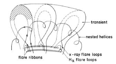
Figure 1.: Left: one of Bruzek’s (1964) sketches, showing a flare with ribbons on the disk and its equivalent H$\alpha$ “loop prominence system” over the limb. This key observational pattern led directly to the formation of our standard flare model (right), in the form presented by Anzer & Pneuman (1982).

In this standard picture a solar flare develops in a complicated manner that involves restructuring of the coronal magnetic field in such a way as to release energy. The immediate effects of this energy release are to produce broad-band “impulsive phase” emissions and to drive chromospheric gas up into coronal magnetic loops, the process we term “chromospheric evaporation.” A part of the field magnetic structure may actually erupt and open out into the solar wind, in the sense that the field lines stretch out past the Alfvé n critical point of the flow. This opening may consist of rising loops which then take the form of a coronal mass ejection (CME), or it may involve interactions with previously open field (a process often termed “interchange reconnection” nowadays; see Heyvaerts et al. (1977)). If a CME does accompany the flare, as it almost invariably does for flares of GOES class X or greater, the energy involved in mass motions may be comparable to the luminous energy (e.g., Emslie et al. (2005)). Generally the observations are limited in resolution, both temporal and spatial, and especially in spectral coverage. Thus we often resort to a cartoon that serves to identify how the essential parts of a flare relate to one another.

Soft X-ray observations show hot loops in the gradual phase of a flare. These result from the material “evaporated” from the chromosphere and have anomalously high gas pressure (but still low plasma $\beta$; however see Gary (2001)). Whereas the pressure at the base of the corona normally is of order 0.1 dyne cm^-2, a bright flare loop can achieve 10³ dyne cm^-2. This over-dense and over-hot coronal loop gradually cools, and in its final stages the remaining plasma returns to a more chromospheric state and suddenly becomes visible in H$\alpha$ (Goldsmith (1971)). The loops that have reached this state then form Bruzek’s H$\alpha$ loop prominence system (Figure 1).

During the ribbon expansion another important phenomenon occurs: hard X-ray emission appears at the footpoints of the coronal loops that are in the process of being filled by chromospheric evaporation (Hoyng et al. 1981). The hard X-rays show that a substantial part of flare energy appears in the form of non-thermal electrons (Kane & Donnelly (1971); Lin & Hudson (1976); Holman et al. (2003)). The hard X-ray signature (and hence the energetic dominance of these electrons) is present whether or not the flare develops the two-ribbon morphology or has a CME association.

The hard X-ray emission occurs in the impulsive phase of the flare, contemporaneously with the period of chromospheric evaporation that fills the coronal loops and with the acceleration phase of the associated CME (Zhang et al. (2001)). In Section 5 we describe this phase of the flare with the thick-target model (Kane & Donnelly (1971)) which Hudson (1972) identified with the energy source of white-light flare continuum.

3 The Flare Spectrum

A (major) flare can be observed at almost any wavelength in a fast-rise/slow-decay time profile, with some (e.g., the white-light continuum) having a more impulsive variability, and others (e.g., the Balmer lines) having a more gradual pattern (Figure 2, right). We generally describe a flare as consisting of a footpoint and ribbon structures in the lower atmosphere, coronal loops, and various kinds of ejecta. The impulsive phase is typically associated with the footpoint structures, and the gradual phase with the flare ribbons. Nowadays imaging spectroscopy in principle allows us to study these regions independently.

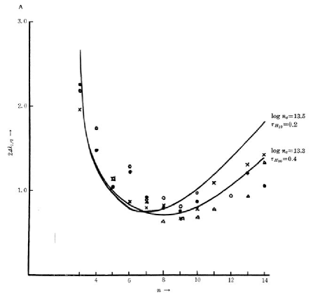
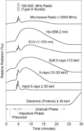
Figure 2.: Left: Line widths of the Balmer-series lines, from the classic paper by Suemoto & Hiei (1959). The inferred densities added to the curves are $\log n_{\rm e}=13.5$ and 13.3; the inferred filling factor is small, suggesting either filamentary structure or thin layering. Right: Typical time series of flare radiations, distinguishing the impulsive phase from the gradual phase (see Kane & Donnelly (1971)).

Flare spectroscopy began with the observation of the Balmer series, which shows broad lines tending towards emission profiles as the flare gets more energetic. Early observations of the higher members of the sequence allowed the inference of a relatively high density and of a small filling factor (Suemoto & Hiei (1959); see the left panel of Figure 2). Such observations refer to what we would now call the gradual phase of the flare (see the right panel of Figure 2 for a sketch of the temporal development of a flare). In the impulsive phase the continuum appears in emission, as noted originally by Carrington and by Hodgson independently. The weak photospheric metallic lines may also go weakly into emission (or are filled in by continuum) and the recent observations of Xu et al. (2004) show that flare effects can appear even at the “opacity minimum” region of the spectrum, where one would expect much higher densities. In fact a single density could never properly describe such a heterogeneous structure, but each spectral band provides its own clues. At the time of writing no proper analysis of spectroscopic “response functions” (e.g., Uitenbroek (2005)) for any of the signatures has yet been attempted, so our inference of flare structure from the spectroscopy alone is weak.

The continuum radiation seen in white light and the UV constitutes the bulk of flare radiated energy (Kane & Donnelly (1971); Woods et al. (2006)). TRACE imaging of this emission component shows it to consist of unresolved, intensely bright fine structures (Hudson et al. (2006)). The thick-target model invokes fast electrons (energies above about 10 keV) to transport coronal energy into the chromosphere. Here collisional losses provide the heating and footpoint emissions that accompany the hard X-ray bremsstrahlung. The thick-target model does not explain the particle acceleration, nor show how the footpoint sources can be so intermittent. We return to this question in Section 7.

The spectra emitted at the footpoints of the flaring coronal loops have contributions over an exceptionally broad wavelength range, as sketched in the right panel of Figure 2. The prototypical observable is the hard X-ray flux, which imaging observations show to be concentrated at the footpoints (Hoyng et al. (1981)), but impulsive footpoint emissions also occur in many spectral windows ranging from the microwaves (limited presumably by opacity) to the $\gamma$-rays (limited presumably by detection sensitivity). There is a large body of work on the H$\alpha$ line alone, both observation and theory. Berlicki (2007) reviews the H$\alpha$ spectroscopic material in detail in these proceedings. A strong absorption line forms across a wide range of continuum optical depths, and in principle this single line might provide sufficient information to infer the physical structure of the flare everywhere. In practice the complexities of the radiative transfer and of the flare motions, especially in the impulsive phase, make this information ambiguous (see Berlicki 2007).

4 Chromospheric Evaporation

The motions most directly relevant to the chromosphere are often called “chromospheric evaporation,” even though the direct Doppler signatures of this motion are normally found in lines formed at higher temperatures (but see Berlicki et al. (2005)). That this process occurs (even if it is not “evaporation” strictly speaking) was suggested by the early observations of loop prominence systems (e.g., Bruzek (1964)) with their “coronal rain,” and Neupert (1968) established its association with non-thermal processes such as bursts of microwave synchrotron radiation. The thermal microwave spectrum (e.g., Hudson & Ohki (1972)) made it particularly clear that the gradual phase of a solar flare involves the temporary levitation of chromospheric material into the corona, as opposed to the process that might be imagined from the earlier term “sporadic coronal condensation” (e.g., Waldmeier (1963)). The flows involved in chromospheric evaporation are along the field direction and serve to create systems of coronal loops with relatively high gas pressure and therefore higher (but still probably low) plasma beta.

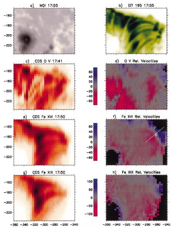
Figure 3.: Imaging spectroscopy from SOHO/CDS of EUV emission lines in the gradual phase of a two-ribbon flare, showing the clear signature of blueshifted upflows in the expected locations along the flare ribbons. This is “gentle” evaporation not associated with strong hard X-ray emission (from Czaykowska et al. (1999)). Note that CDS produces images by scanning in one spatial dimension, so that each image (while monochromatic) is not instantaneous.

The early observational indications of chromospheric evaporation actually came from blueshifts in EUV and soft X-ray lines (e.g., Antonucci et al. (1982); Acton et al. (1982)) such as those from Fe XXV or Ca XIX. Figure 3 shows an image-resolved view of Doppler shifts in an evaporative flow (Czaykowska et al. (1999)). The chromospheric effects are more subtle and in fact the impulsive-phase evaporation is difficult to disentangle from other effects (Schmieder et al. (1987)). The high-temperature blueshifts correspond to upward velocities of some hundreds km/s and seldom appear in the absence of a stationary emission line; in other words, hot plasma has already accumulated in coronal loops as the process continues. Based on theory and simulations (Fisher et al. (1985)) one can distinguish “explosive” and “gentle” evaporation, depending upon the physics of energy deposition (e.g., Abbett & Hawley 1999). In explosive evaporation, driven hypothetically by an electron beam, one has the additional complication of a “chromospheric condensation” that produces a redshift as well. Schmieder et al. (1987) and Berlicki et al. (2005) survey our overall understanding. It would be fair to comment that the explosive evaporation stage remains ill-understood, even though it principle it describes the key physics of sudden mass injections into flare loops.

5 Energetics and Magnetic Field

We can use the standard VAL-C model (Vernazza et al. 1981), as discussed further in the Appendix, to discuss the energetics. First we establish that the chromosphere and the rest of the lower solar atmosphere (i.e., that for which $\tau_{5000}<1$) have negligible heat capacity and limited time scales. Figure 4 shows an estimate of the radiative time scale in the VAL-C model (Vernazza et al. (1981)). This shows 3$\sigma(z)kT/{\mathcal{L}}_{\odot}$, where $\sigma$ is the surface density as a function of height about the $\tau_{5000}$ = 1 layer, and ${\mathcal{L}}_{\odot}$ the solar luminosity. The time scale decreases below 1 sec only above z $\sim$ 515 km, near the temperature minimum in the VAL-C model. Above this height any energy injected into the system will tend to radiate rapidly, resulting in a direct energy balance between input and output energy, rather than a local storage and release. At lower altitudes we would not expect to see rapid variability.

Figure 4.: Characteristic radiative cooling time (upper) as a function of height in the VAL-C model, crudely estimated as described in the text. The lower panel shows the temperature in this model.

The model also allows us to ask whether the chromosphere itself can store energy comparable to that released in a major flare or CME. Table 1 gives some order-of-magnitude properties for a chromospheric area of 10¹⁹ cm², showing both possible sources (bold) and sinks (italics) of energy. For the magnetic field we simply assume 10 or 1000 G as representative cases. Using the total magnetic energy in this manner is an upper limit, since the actual free energy would depend on its degree of non-potentiality. We find that magnetic energy storage limited to the volume of the chromosphere will not suffice, unless unobservably small-scale fields there somehow dominate. The gravitational potential energy also will not suffice. Estimates of this sort confirm the idea that the flare energy must reside in the corona prior to the event.

The estimate of gravitational potential energy is somewhat more ambiguous. The Table shows the value needed to displace the entire atmosphere by its total thickness, the equivalent of roughly 3^′′ in the VAL-C model. There does not seem to be any evidence for such a displacement, although I am not aware of any searches. It is likely that the stresses that store energy in the coronal field have their origin deeper in the convection zone, rather than in the atmosphere (McClymont & Fisher 1989). Actually the observable changes of gravitational energy are even of the wrong sign, given that we normally observe only outward motions, (against gravity) during a flare.

Table 1.: Properties of a chromospheric volume of area 10¹⁹ cm²

Parameter	VAL-C	VAL-C above Tmin
Mass	4$\times$1019 gram	5$\times$1017 gram
Magnetic energy	1$\times$1028erg	8$\times$1027 erg (10 G)
Magnetic energy	1$\times$1032 erg	8$\times$1031 erg (103 G)
Gravitational energya	3$\times$1032 erg	3$\times$1030 erg
Thermal energy	2$\times$1031 erg	3$\times$1029 erg
Kinetic energy	3$\times$1029 erg	3$\times$1027 erg
Ionization energy	4$\times$1032 erg	6$\times$1030 erg

^aPotential energy for a vertical displacement of 2.5 $\times$ 10⁸ cm

From Table 1 one concludes that the chromosphere probably does play a dominant role in the energetics of a solar flare, at least as described by a semi-empirical model such as VAL-C. This just restates the conventional wisdom, namely that the flare energy needs to be stored magnetically in the corona, rather than in the chromosphere where the radiation forms. Note that this is backwards from the relationship for steady emissions: the requirement for chromospheric heating is larger than that for coronal heating, so it is possible to argue that the steady-state corona actually forms as a result of energy leakage from the process of chromospheric heating (e.g., Scudder (1994)).

We can make a similar estimate for energy flowing up from the photosphere. The Alfvén speed at $\tau_{5000}$ = 1 ranges from 3 to 30 km s^-1, depending on the field strength, in the VAL-C model (see Appendix). Below the surface of the Sun $v_{A}$ drops rapidly because of the increase of hydrogen ionization. Thus chromospheric flare energy cannot have been stored just below the photosphere, since it could not propagate upwards rapidly enough (McClymont & Fisher 1989). This again supports the conventional wisdom that flare energy resides in the corona prior to the event.

To drive chromospheric radiations from coronal energy sources requires efficient energy transport, which is normally thought to be in the form of non-thermal particles (the “thick target model”, Brown 1971; Hudson 1972) or in the form of thermal conduction as in the formation of the classical transition region. Both of these mechanisms provide interesting physical problems, but the impulsive phase of the flare (where the thick-target model usually is thought to apply) certainly remains less understood. Section 11 comments on models.

The magnetic field in the chromosphere is decisively important but ill-understood. The plasma beta is generally low (see Appendix), so just as in the corona the dynamics depends more on the behavior of the field itself than to the other forces at work. Generally we believe that the subphotospheric field exists in fibrils, implying the existence of sheath currents that isolate the flux tubes from their unmagnetized environment. On the other hand, the dominance of plasma pressure in the chromosphere as well as the corona implies that the field must rapidly expand to become space-filling. Longcope & Welsch (2000) discuss the physics involved in this process as flux emerges from the interior. The effect of the flux emergence must be to create current systems linking the sources of magnetic stress below the photosphere, with the non-potential fields containing the coronal free energy. A full theory of how this works does not exist, and we must add to the uncertainty the possibilty of unresolved fields (e.g., Trujillo Bueno et al. 2004). Their suggested factor of 100 in B² would clearly affect the estimate of magnetic energy given in Table 1 and perhaps change everything. We note in this context that the “impulse response” flares (White et al. 1992) have scales so small that one could argue for an entirely chromospheric origin.

6 Energetics and the Formation of the Continuum

The formation of the optical/UV emission spectrum of a solar flare has from the outset presented a special challenge, since (a) it represents so much energy, and (b) it appears in what should be the stablest layer of the solar atmosphere. The recent observations of rapid variability and spatial intermittency make this all the more interesting, and these observations – now from space – also help to intercompare events; previous catalogs of white-light flares (e.g., Neidig (1989) and references therein) had to be based on spotty observations made with a wide variety of instruments. Observationally, the continuum appears to have two classes, with most events (“Type I” spectra) showing evidence for recombination radiation via the presence of the Balmer edge and sometimes the Paschen edge as well. A few events (e.g., Machado & Rust (1974)) show spectra with weak or unobservable Balmer jumps, implicating H^- continuum as observed in normal photospheric radiation. The spectra in the latter class (“Type II”) suggests a relationship to Ellerman bombs (Chen et al. (2001)). However, the physics of Ellerman bombs appears to be quite different from that of solar flares (e.g., Pariat et al. 2004), though.

The strong suggestion from correlations is that non-thermal electrons physically transport flare energy from the corona, where it had been stored in the current systems of non-potential field structures, into the radiating layers. The hard X-ray bremsstrahlung results from the collisional energy losses of these particles, and other signatures (such as the optical/UV continuum) depends on secondary effects. Proposed mechanisms include direct heating, heating in the presence of non-thermal ionization, and radiative backwarming. In some manner these effects (or others not imagined) must provide the emissivity $\epsilon_{\nu}$, to support the observed spectrum. Note that the emissivity is often expressed in terms of the source function $S_{\nu}$ = $\epsilon_{\nu}/\kappa_{\nu}$ via the opacity $\kappa_{\nu}$. In a steady state one would have energy balance between the input (e.g., electrons) and the continuum. Fletcher et al. (2007) have now shown that this implies energy transport by low-energy electrons, below 25 keV, as opposed to the 50 keV or higher suggested by some earlier authors. Such low-energy electrons have little penetrating power and could not directly heat the photosphere itself from a coronal acceleration site. Thus either the continuum arises from altered conditions in the chromosphere, or some mechanism must be devised to link the chromosphere and photosphere not involving the thick-target electrons.

“Radiative backwarming” – for example Balmer and Paschen continuum excited in the chromosphere and then penetrating down to and heating a deeper layer – could in principle provide a vertical step between energy source and sink. One problem with this is that the weaker backwarming energy fluxes might not cause appreciable heating in the denser atmosphere, and thus not be able to contribute to the observed continuum excess, because of the short radiative time scale. This idea is a variant of the mechanism of non-thermal ionization originally proposed by Hudson (1972) in the “specific ionization approximation,” which involves no radiative-transfer theory and simply assumes ion-electron pairs to be created locally at a mean energy ($\sim$30 eV per ion pair). Finally, the rapid variability observed in the continuuum, even at 1.56 $\mu$m (Xu et al. 2006) provides a clear argument that the continuum forms at the temperature minimum or above (see Section 5, especially Figure 4).

Early proponents of particle heating as an explanation for white-light flares also considered protons as an energy source (Najita & Orrall (1970); Švestka (1970)). This made sense, because protons at energies even below those characteristic of $\gamma$-ray emission-line excitation can penetrate more deeply than the electrons that produce hard X rays. It makes even more sense now that we have the suggestion that ion acceleration in solar flares may rival electron acceleration energetically (Ramaty et al. (1995)). Simnett & Haines (1990) suggest that particle acceleration in solar flares involves a neutral beam, implying that the major energy content (and hence the optical/UV continuum) would originate in the ion component. This idea does not appear to explain the apparent simultaneity of the footpoint sources (Sakao et al. (1996)), and at present we do not understand the plasma physics of the particle acceleration and propagation well enough even to identify the location of the acceleration region.

7 Flare Structures Inferred from Chromospheric Signatures

The continuum kernels may move systematically for perhaps tens of seconds and generally have short lifetimes. We illustrate this in Figure 5 (from Fletcher et al. (2004)). This shows the motions of individual UV bright points within the flare ribbon structure. Such motions are only apparent motions, as in a deflagration wave, because they exceed the estimated photospheric Alfvén speed (see Section 4 and the Appendix). Figure 6 (from Hudson et al. (2006)) makes the same point for a different flare, using TRACE white-light observations. The basic picture one gets from such observations is that the white light/UV continuum of a flare appears in compact structures that are essentially unresolved in space and in time within the present observational limits. These bright points contain enormous energy and thus must map directly to the energy source. We do not know if the fragmentation (intermittency) results from this mapping or is intrinsic to the basic energy-release mechanism.

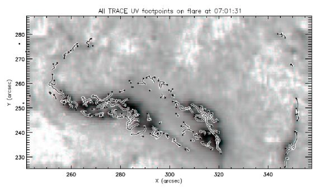
Figure 5.: Flare footpoint apparent motions deduced from TRACE UV observations. Each squiggle represents the track of a bright point visible for several consecutive images at a few-second cadence, with the black dot showing the beginning of each track (Fletcher et al. 2004).

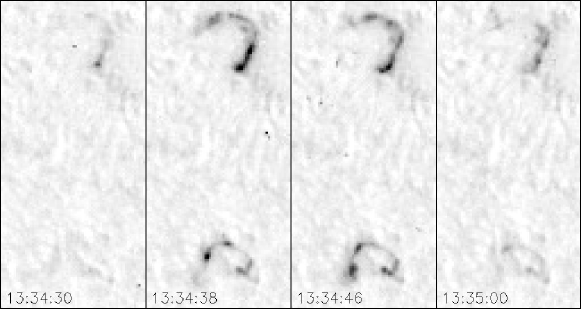
Figure 6.: Intermittent structure seen in TRACE white-light images of an M-class flare on July 24, 2004. The individual frames have dimensions 32${}^{\prime\prime}\times\$64^′′. Note the presence of bright features consistent with the TRACE angular resolution, and which change from frame to frame over the 30-second interval. These observations do not appear to resolve the fluctuations either in space or in time (Hudson et al. 2006).

How do the small chromospheric sources map into the corona, where the flare energy must reside on a large scale before its release? A strong literature has grown up regarding this point, interpreting the ribbon motions as measures of flux transfer in the standard magnetic-reconnection model (Poletto & Kopp (1986); see also literature cited, for example, by Isobe et al. (2005)). The flux transfer in the photosphere is taken to measure the coronal inflow into the reconnecting current sheet, which appears to correlate with the radiated energy as seen in hard X-rays, UV, or H$\alpha$. Figure 1 (right) shows the assumed geometry linking the chromosphere and corona. The analysis extends to the multiple simultaneous UV footpoints apparently moving within the ribbons as they evolve, as noted in Figure 5 above. The analyses suggest a strong relationship between energy release and the inferred coronal Alfvén speed.

8 Dynamics and Magnetic Reconnection

To release energy from coronal magnetic field in a largely “frozen-field” plasma, a flare must involve mass motions. We often do observe apparent motions, both parallel and perpendicular to the field as indicated by the image striations (“loops”). Most of the observable motions are outward, leading to the idea of a “magnetic explosion” (e.g., Moore et al. (2001)). Motions apparently perpendicular to the magnetic field may become coronal mass ejections (CMEs) and contain a great deal of energy (e.g., Emslie et al. (2005)). These perpendicular motions also are involved in flare energy release; for example the large-scale magnetic reconnection involved in many flare models (Figure 1, right panel) necessarily involve “shrinkage” (e.g., Švestka et al. (1987); Forbes & Acton (1996)). Note that this process is more of a magnetic implosion than a magnetic explosion (Hudson 2000).

The motion of flare footpoints and ribbons is (we believe) only apparent, because of the low Alfvén speed $v_{A}$ in the photosphere, where the field is temporarily anchored (“line-tied”). For $B$ =1000 G and $n$ = 10¹⁷ cm^-3 we find $v_{A}\sim$ 6 km s^-1; observations often suggest motions an order of magnitude faster (e.g., Schrijver et al. 2006). The motions therefore represent a wave-light conflagration moving through a relatively fixed magnetic-field structure. It is natural to imagine that this sequence of field lines links to the coronal energy-release site, which the standard model identifies with a current sheet that mediates large-scale magnetic reconnection.

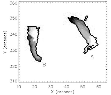
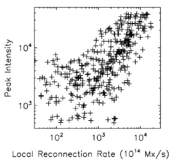
Figure 7.: Left: UV ribbons (TRACE observations) from a flare of November 23, 2000. The gray scale shows the time sequence of brightening. Right: Correlation between pixel brightness in Ribbon A and the inferred reconnection rate (from Saba et al. (2006)).

Figure 7 shows one example of the result of an analysis of the apparent motion of a flare ribbon (Saba et al. 2006). This and other similar analyses reveal a tendency for the “reconnection rate” to correlate with the pixel brightness. The reconnection rate is the rate at which flux is swept out in the ribbon motion, often expressed as an electric field from E = v$\times$B (the so-called “reconnection electric field”). In this picture the flare ribbons are identified with “quasi-separatrix structures” where magnetic reconnection can take place most directly.

9 Surges, Sprays, and Jets

Chromospheric material also appears in the corona in the form of surges and sprays, which may have a close relationship to the flare process (e.g., Engvold 1980). In addition, of course, we observe filaments and prominences in chromospheric lines, and these also have a flare/CME association, but too tangential for discussion in this review.

Surges and sprays are H$\alpha$ ejecta, rising into the corona as a result of chromospheric magnetic activity. The literature traditionally distinguishes them by apparent velocity, with the faster-moving sprays taken to have stronger flare associations. Surges often appear to return to the Sun, while sprays accelerate beyond the escape velocity and do not return. Both appear to move along the magnetic field lines, but unlike the evaporation flow the surges and sprays incorporate material at chromospheric temperatures.

Modern soft X-ray and EUV data (Yohkoh, SOHO, and TRACE) have had sufficient time resolution to reveal the phenomenon of X-ray jets (Shibata et al. 1992); see also the UV observations of Dere et al. (1983). These tightly-collimated structures at X-ray temperatures have a strong correlation with surges and sprays, and indeed presumably lead to the jet-like CMEs seen at much greater altitudes (Wang & Sheeley 2002). These events have a strong association with emerging flux, and indeed the X-ray jets invariably have an association with microflares and originate in the chromosphere near the microflare loop(s) (Shibata et al. 1992). As Zirin famously remarked, most emerging flux emerges within active regions, and that is where the jets preferentially occur. The site is frequently in the leading part of the sunspot group. Figure 8 (Canfield et al. 1996) shows the sequence of events in an explanation of these phenomena invoking magnetic reconnection to allow chromospheric material access to open fields. Note that this scenario imposes two requirements on the chromosphere: there must be open and closed fields juxtaposed, and a large-scale reconnection process must be able to proceed under chromospheric conditions. The Canfield et al. (1996) observations strongly imply that this process requires the presence of vertical electric currents supporting the observed twisting motions.

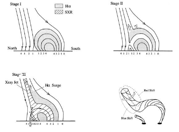
Figure 8.: A mechanism for jet/surge formation involving emerging flux (upper left), with magnetic reconnection against already-open fields (upper right), which may lead to a high-temperature ejection (the jet) entraining chromospheric material (the surge). The cartoon at lower right describes the observations of (Canfield et al. 1996), who find a spinning motion suggesting that the process must occur in a 3D configuration rather than that of the cartoons left and above.

The surges, sprays, and jets, not to mention flares and CMEs, underscore the time dependence and three-dimensionality characterizing what is often characterized as a thin time-independent layer for convenience. The subject of spicules is outside the scope of this review, but we note that they represent a form of activity that occurs ubiquitously outside the magnetic active regions.

10 A Chromospheric $\gamma$-ray Mystery

The $\gamma$-ray observations of solar flares have begun, as did the radio and X-ray observations before them, to open new windows on flare physics. Share et al. (2004) have made a discovery that is difficult to understand and which involves chromospheric material. They report observations of the line width of the 0.511 MeV $\gamma$-ray emission line formed by positron annihilation (Figure 9). This emission requires a complicated chain of events: the acceleration of high-energy ions, their collisional braking and nuclear interactions in the solar atmosphere, the emission of secondary positrons by the excited nuclei, the collisional braking of these energetic positrons in turn, and finally their recombination with ambient electrons to produce the 0.511 MeV $\gamma$-rays. Because the $\gamma$-ray observations are so insensitive, this process requires an energetically significant level of particle acceleration that is possibly distinct from the well-known electron acceleration in the impulsive phase.

Figure 9.: RHESSI $\gamma$-ray observations of the 0.511 MeV line of positron annihilation (Share et al. (2004)). The two line profiles are from different integrations in the late phase of the X17 flare of 28 October 2003; for the broader line the authors suggest thermal broadening, which would require a large column depth of transition-region temperatures during the flare.

The mystery comes in the line width of the emission line. Surprisingly the pioneering RHESSI observations of Share et al. (2004) showed it to be broad enough to resolve. The likeliest source of this line broadening is Doppler motions in the positron-annihilation region. This requires the existence of a large column density (of order gram cm^-2) at transition-region temperatures; the transition region under hydrostatic conditions would be many orders of magnitude thinner (see also Figure 11). According to Schrijver et al. (2006), the excitation of the footpoint regions during the the time of intense particle acceleration only continues for some tens of seconds at most. This would represent the time scale for the apparent motion of a foopoint source across its diameter. The $\gamma$-ray observations, on the other hand, require minutes of integration for a statistically significant line-profile measurement.

We therefore are confronted with a major problem. What is the structure of the flaring atmosphere that permits the formation of the broad 0.511 MeV $\gamma$-ray line? Recent spectroscopic observations of the impulsive phase in the UV, as viewed off the limb (Raymond et al. 2007) make a conventional explanation difficult.

11 Theory and Modeling

To understand the chromospheric spectrum of a solar flare we must understand the formation of the radiation and its transfer in the context of the motions produced by (or producing) the flare. The representation of the spectrum by a “semi-empirical model” represents one shortcut; in such an approach (e.g., the standard VAL model that we use in the Appendix) one attempts to construct a model atmosphere capable of describing the spectrum even if it may not be physically self-consistent. Such descriptions may however be sufficient in the gradual phase of a flare when the flare loops no longer have energy input and simply evolve by cooling and draining. Even here, however, we do not have a good understanding of the “moss” regions that form at the footpoints of these high-pressure loops (but see Berger et al. (1999)). So far as I am aware there is no literature specifically on “spreading moss,” the similar structure that appears in association with flare ribbons.

A more complete approach to the physics comes from “radiation hydrodynamics” physical models, most recently those of Allred et al. (2005); see Berlicki (2007) for a fuller description. Such models solve the equations of hydrodynamics and radiative transfer simultaneously and can thus deal with chromospheric evaporation and the formation of the high-pressure flare loops. This framework is necessary if we are to be able to understand the flare impulsive phase (e.g., Heinzel 2003). Even these models do not have sufficient realism, though, since they work currently in one dimension and thus cannot follow the time development of the excitation properly; the high-resolution observations of UV and white light by TRACE clearly show that the energy release has unresolved scales. Further, as pointed out by Hudson (1972), the ionization of the chromosphere (and hence the formation of the continua) cannot be described by a fluid approximation, or even by non-LTE radiative transfer that assumes a unique temperature.

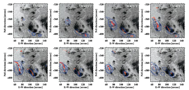
Figure 10.: Continuum emission in the near infrared (1.56 $\mu$m, the “opacity minimum” region) during an X10 flare (Xu et al. (2004)). Red shows the IR emissions, contours show the RHESSI 50-100 keV X-ray sources. The IR contrast relative to the preflare photosphere reached $\sim$20% in this event.

At present there has been little effort to create an electrodynamic theory of chromospheric flare processes, even though non-thermal particles are widely thought to provide the dominant energy in at least the impulsive phase. In the gradual phase there is interesting physics associated with heat conduction because the transition region would have to become so steep that classical conductivity estimates have difficulty (Shoub (1983)). A more complete theory would have to take plasma effects into account and would probably contain elements of theories of the terrestrial aurora that are now largely missing from the solar lexicon. This lack of self-consistency in the modeling probably means that we have major gaps in our understanding of, for example, the evaporation process as it affects the fractionation of the elements and of the ionization states of the flare plasma. The Appendix gives estimates of the ranges of some the key plasma parameters in the chromosphere.

12 Conclusions

This article has reviewed chromospheric flare observations from the point of view of the newest available information – Yohkoh, SOHO, TRACE and RHESSI, for example, but not Hinode or STEREO (already launched), nor much less FASR or ATST (not launched yet at the time of writing). spite of the high quality of the data prior to these missions, we still find major unsolved problems:

$\bullet$ How does the chromosphere obtain all of the energy that it radiates?

$\bullet$ How can flare effects appear at great depths in the photosphere?

$\bullet$ How is the anomalous 0.511 MeV line width produced?

$\bullet$ What are the elements of an electrodynamic theory of chromospheric flares?

In my view the solution of these problems cannot be found in chromospheric observations alone, because the physical processes involve much broader regions of the solar atmosphere. Even providing answers to these specific questions may not reveal the plasma physics responsible for flare occurrence, which may involve spatial scales too fine ever to resolve. But we can hope that new observations from space and from the ground, in wavelengths ranging from the radio to the $\gamma$-rays, will enable us to continue our current rapid progress, and can speculate that eventually numerical tools will supplement the theory well enough for us to achieve full comprehension of the important properties of flares. To get to this point we will need to deal with the chromosphere, as messy as it is.

One important task that is probably within our grasp now is the computation of response functions for physical models of flares. At present these are restricted to very limited numerical explorations of the radiative transfer within the framework of one-dimensional radiation hydrodynamics (e.g., Allred et al. (2005)). The energy transport in these models has been restricted to simplistic representations of particle beams for energy transport, and do not take account of complicated flare geometries, waves, or various elements of plasma physics. Future developments of chromospheric flare theory will need to complete the picture in a more self-consistent manner.

Acknowledgments This work has been supported by NASA under grant NAG5-12878 and contract NAS5-38099. I thank W. Abbett for a critical reading. I am also grateful to Rob Rutten for LaTeX instruction, and to Bart de Pontieu for meticulous keyboard entry.

Appendix: plasma parameters

The lower solar atmosphere marks the transition layer between regions of striking physical differences, and as one goes further up in height the tools of plasma physics should become more important. This Appendix evaluates for convenience several basic plasma-physics parameters for the conditions of the staple VAL-C atmospheric model (Vernazza et al. 1981). This is a “semi-empirical model” in which interprets a set of observations in terms of the theory of radiative transfer, but without any effort to have self-consistent physics. Such a model can accurately represent the spectrum but may or may not provide a good starting point for physical analysis. Because the optical depth of a spectral feature is the key parameter determining its structure, one often sees the model parameters plotted against continuum optical depth $\tau_{5000}$ evaluated at 5000Å. Just for illustration, Figure 11 shows the VAL-C temperature separately as a function of height, column mass, and optical depth. Note that features prominent in one display may appear to be negligible in another

Figure 11.: Illustration of the structure of a semi-empirical model, using three different independent variables: the VAL-C temperature plotted against height, optical depth, and column mass.

The VAL-C model is an “average quiet Sun” model, and like all static 1D models, it cannot describe the variability of the physical parameters that theory and observation require (see other papers in these proceedings, e.g., Carlsson’s review). Thus we should regard the plasma parameters estimated here as order-of-magnitude estimates only and note especially that the vertical scales, which depend in the model on the inferred optical-depth scale, may be systematically displaced.

The VAL-C model explicitly does not represent a chromosphere perturbed by a flare. Vernazza et al. (1981) and many other authors give more appropriate models derived by similar techniques for flares as well as other structures. As the discussion of the $\gamma$-ray signatures in Section 10 suggests, though, a powerful flare may be able distort the lower solar atmosphere essentially beyond all recognition (especially in the impulsive phase). To estimate representative plasma parameters I have therefore chosen just to start with the basic VAL-C model, and we simply assume constant values of $B$ at 10 G and 1000 G. The actual magnetic field may vary through this region (the “canopy”) but the details are little-understood. The $\gamma$-ray literature usually uses a parametrization of the magnetic field strength $B\propto P_{g}^{\alpha}$ (Zweibel & Haber (1983)), where $P_{g}$ is the gas pressure.

The most complicated behavior of the plasma parameters happens preferentially near the top of the VAL-C model range (for example, Figure 12 shows that the collision frequency decreases below the plasma and Larmor frequencies) above the helium ionization level (or even below this level for strong magnetic fields). Because VAL-C ignores time dependences and 3D structure, and assumes $T_{e}=T_{i}$, we can expect that it has diminished fidelity as one approaches the unstable transition region; thus one should be especially careful not to take these approximations too literally. The following notes correspond to each panel of the figure. Most of the plasma-physics formulae used in this Appendix are from Chen (1984).

Figure 12.: Various plasma parameters in the VAL-C model. We have assumed representative $B$ values of 10 G and 1000 G. The different panels show the following, left to right and top to bottom: (a) Temperature. (b) Densities: solid, total hydrogen density; dotted, electron density; dashed, He I density; dash-dot, He II density. (c) Plasma beta: solid, for 1000 G; dotted, for 10 G; light solid, electron density as a fraction of total hydrogen density; dash-dot, the plasma parameter. (d) Frequencies. Solid, electron and ion plasma frequencies; dotted, electron gyrofrequencies for 10 and 1000 G; dashed, electron and ion collision frequencies; dash-dot, electron/neutral collision frequency. (e) Velocities: Solid, electron and ion thermal velocities; dashed, Alfvén speeds for 10 and 1000 G. (f) Scale lengths: solid, electron Larmor radii for 10 G and 100 G; dotted, Debye length; dashed, ion and electron inertial lengths.

Temperature: The VAL-C model, like all of the semi-empirical models, sets T_e = T_i. It therefore cannot support plasma processes dependent upon different ion and electron temperatures, or more complicated particle distribution functions (e.g. Scudder 1994).

Densities: Total hydrogen density, electron density, and densities of He I and He II.

Dimensionless parameters: We approximate the plasma beta as

$$\beta={{{2(n_{H}+2n_{e})kT}}\over{B^{2}/8\pi}}$$

with $n_{H}$ the hydrogen density, $n_{e}$ the electron density, Figure 12(c) gives the number of electrons in a Debye sphere as the “plasma parameter” $\Lambda$.

Frequencies: The plasma frequency, the electron and proton Larmor frequencies, and the electron and ion and collision frequencies

$$\nu_{ei}=2.4\times 10^{-6}n_{e}ln\Lambda/T_{eV}^{3/2};\ \ \ \nu_{ii}=0.05\times 4\nu_{ei};\ \ \ \nu_{eH}=(n_{H}/n_{e})\nu_{e}$$

with $n_{e}$ in cm^-3, $T_{eV}$ the temperature in eV, using Z = 1.2 and the Coulomb logarithm ln$\Lambda$ = 23 - ln(n${}_{e}^{0.5}$T${}_{eV}^{-1.5}$) (Chen 1984; De Pontieu et al. 2001).

Note that the collision frequencies are small compared with the plasma and Larmor frequencies above about 1000 km in this model. This means generally that plasma processes must have strong effects on the physical parameters of the atmosphere in this region.

Velocities: Electron and proton thermal velocities; Alfvén speeds $v_{A}$ for 10 and 1000 G.

Scale lengths: Electron Larmor radii for 10 and 1000 G, the ion inertial length $c/\omega_{pi}$, the electron inertial length $c/\omega_{pe}$, and the Debye length $\lambda_{D}$. The inertial lengths determines the scale for the particle demagnetization necessary for magnetic reconnection. For VAL-C parameters the ion inertial length increases to about 100 m in the transition region.

References

- Abbett & Hawley (1999) Abbett W. P., Hawley S. L., 1999, ApJ521, 906
- Acton et al. (1982) Acton L. W., Leibacher J. W., Canfield R. C., Gunkler T. A., Hudson H. S., Kiplinger A. L., 1982, ApJ263, 409
- Allred et al. (2005) Allred J. C., Hawley S. L., Abbett W. P., Carlsson M., 2005, ApJ630, 573
- Antonucci et al. (1982) Antonucci E., Gabriel A. H., Acton L. W., Leibacher J. W., Culhane J. L., Rapley C. G., Doyle J. G., Machado M. E., Orwig L. E., 1982, Solar Phys.78, 107
- Anzer & Pneuman (1982) Anzer U., Pneuman G. W., 1982, Solar Phys.79, 129
- Berger et al. (1999) Berger T. E., de Pontieu B., Fletcher L., Schrijver C. J., Tarbell T. D., Title A. M., 1999, Solar Phys.190, 409
- Berlicki et al. (2005) Berlicki A., Heinzel P., Schmieder B., Mein P., Mein N., 2005, A&A430, 679
- Berlicki (2007) Berlicki A., 2007, these proceedings
- Brown (1971) Brown J. C., 1971, Solar Phys.18, 489
- Bruzek (1964) Bruzek A., 1964, ApJ140, 746
- Canfield et al. (1996) Canfield R. C., Reardon K. P., Leka K. D., Shibata K., Yokoyama T., Shimojo M., 1996, ApJ464, 1016
- Chen (1984) Chen F. F., 1984, Introduction to plasma physics, 2nd edition, New York: Plenum Press, 1984
- Chen et al. (2001) Chen P.-F., Fang C., Ding M.-D., 2001, Chinese Journal of Astronomy and Astrophysics 1, 176
- Czaykowska et al. (1999) Czaykowska A., de Pontieu B., Alexander D., Rank G., 1999, ApJ521, L75
- De Pontieu et al. (2001) De Pontieu B., Martens P. C. H., Hudson H. S., 2001, ApJ558, 859
- Dere et al. (1983) Dere K. P., Bartoe J.-D. F., Brueckner G. E., 1983, ApJ 267, L65
- Emslie et al. (2005) Emslie A. G., Dennis B. R., Holman G. D., Hudson H. S., 2005, Journal of Geophysical Research (Space Physics) 110, 11103
- Engvold (1980) Engvold O., 1980, in M. Dryer, E. Tandberg-Hanssen (eds.), IAU Symp. 91: Solar and Interplanetary Dynamics, p. 173
- Fisher et al. (1985) Fisher G. H., Canfield R. C., McClymont A. N., 1985, ApJ289, 434
- Fletcher et al. (2004) Fletcher L., Pollock J. A., Potts H. E., 2004, Solar Phys.222, 279
- Forbes & Acton (1996) Forbes T. G., Acton L. W., 1996, ApJ459, 330
- Gary (2001) Gary G. A., 2001, Solar Phys.203, 71
- Goldsmith (1971) Goldsmith D. W., 1971, Solar Phys.19, 86
- Hale (1930) Hale G. E., 1930, ApJ71, 73
- Handy et al. (1999) Handy B. N. et al., 1999, Solar Phys. 187, 229
- Heinzel (2003) Heinzel P., 2003, Advances in Space Research 32, 2393
- Heyvaerts et al. (1977) Heyvaerts J., Priest E. R., Rust D. M., 1977, ApJ216, 123
- Holman et al. (2003) Holman G. D., Sui L., Schwartz R. A., Emslie A. G., 2003, ApJ595, L97
- Hoyng et al. (1981) Hoyng P. et al., 1981, ApJ246, L155
- Hudson (1972) Hudson H. S., 1972, Solar Phys.24, 414
- Hudson (2000) Hudson H. S., 2000, ApJ 531, L75
- Hudson & Ohki (1972) Hudson H. S., Ohki K., 1972, Solar Phys.23, 155
- Hudson et al. (2006) Hudson H. S., Wolfson C. J., Metcalf T. R., 2006, Solar Phys.234, 79
- Isobe et al. (2005) Isobe H., Takasaki H., Shibata K., 2005, ApJ632, 1184
- Kane & Donnelly (1971) Kane S. R., Donnelly R. F., 1971, ApJ164, 151
- Lin et al. (2002) Lin R. P., et al., 2002, Solar Phys.210, 3
- Lin & Hudson (1976) Lin R. P., Hudson H. S., 1976, Solar Phys.50, 153
- Longcope & Welsch (2000) Longcope D. W., Welsch B. T., 2000, ApJ545, 1089
- Machado & Rust (1974) Machado M. E., Rust D. M., 1974, Solar Phys.38, 499
- McClymont & Fisher (1989) McClymont A. N., Fisher G. H., 1989, in J. H. Waite Jr., J. L. Burch, R. L. Moore (eds.), Solar System Plasma Physics, p. 219
- Moore et al. (2001) Moore R. L., Sterling A. C., Hudson H. S., Lemen J. R., 2001, ApJ552, 833
- Najita & Orrall (1970) Najita K., Orrall F. Q., 1970, Solar Phys.15, 176
- Neidig (1989) Neidig D. F., 1989, Solar Phys.121, 261
- Neupert (1968) Neupert W. M., 1968, ApJ 153, L59
- Pariat et al. (2004) Pariat E., Aulanier G., Schmieder B., Georgoulis M. K., Rust D. M., Bernasconi P. N., 2004, ApJ614, 1099
- Poletto & Kopp (1986) Poletto G., Kopp R. A., 1986, in The Lower Atmosphere of Solar Flares, p. 453
- Ramaty et al. (1995) Ramaty R., Mandzhavidze N., Kozlovsky B., Murphy R. J., 1995, ApJ455, L193
- Raymond et al. (2007) Raymond J. C., Holman G., Ciaravella A., Panasyuk A., Ko Y. ., Kohl J., 2007, ArXiv Astrophysics e-prints 1359
- Saba et al. (2006) Saba J. L. R., Gaeng T., Tarbell T. D., 2006, ApJ641, 1197
- Sakao et al. (1996) Sakao T., Kosugi T., Masuda S., Yaji K., Inda-Koide M., Makishima K., 1996, Advances in Space Research 17, 67
- Schmieder et al. (1987) Schmieder B., Forbes T. G., Malherbe J. M., Machado M. E., 1987, ApJ317, 956
- Schrijver et al. (2006) Schrijver C. J., Hudson H. S., Murphy R. J., Share G. H., Tarbell T. D., 2006, ApJ650, 1184
- Scudder (1994) Scudder J. D., 1994, ApJ427, 446
- Share et al. (2004) Share G. H., Murphy R. J., Smith D. M., Schwartz R. A., Lin R. P., 2004, ApJ615, L169
- Shibata et al. (1992) Shibata K., et al., 1992, PASJ44, L173
- Shoub (1983) Shoub E. C., 1983, ApJ266, 339
- Simnett & Haines (1990) Simnett G. M., Haines M. G., 1990, Solar Phys.130, 253
- Smith & Smith (1963) Smith H. J., Smith E. V. P., 1963, Solar flares, New York: Macmillan, 1963
- Suemoto & Hiei (1959) Suemoto Z., Hiei E., 1959, PASJ11, 185
- Trujillo Bueno et al. (2004) Trujillo Bueno J., Shchukina N., Asensio Ramos A., 2004, Nat430, 326
- Uitenbroek (2005) Uitenbroek H., 2005, AGU Spring Meeting Abstracts
- Švestka (1966) Švestka Z., 1966, Space Science Reviews 5, 388
- Švestka (1970) Švestka Z., 1970, Solar Phys.13, 471
- Švestka (1976) Švestka Z., 1976, Solar Flares, Dordrecht: Reidel, 1976
- Švestka et al. (1987) Švestka Z. F., Fontenla J. M., Machado M. E., Martin S. F., Neidig D. F., 1987, Solar Phys.108, 237
- Vernazza et al. (1981) Vernazza J. E., Avrett E. H., Loeser R., 1981, ApJS45, 635
- Waldmeier (1963) Waldmeier M., 1963, Zeitschrift fur Astrophysik 56, 291
- Wang & Sheeley (2002) Wang Y.-M., Sheeley, Jr. N. R., 2002, ApJ575, 542
- White et al. (1992) White S. M., Kundu M. R., Bastian T. S., Gary D. E., Hurford G. J., Kucera T., Bieging J. H., 1992, ApJ 384, 656
- Woods et al. (2006) Woods T. N., Kopp G., Chamberlin P. C., 2006, Journal of Geophysical Research (Space Physics) 111, 10
- Xu et al. (2006) Xu Y., Cao W., Liu C., Yang G., Jing J., Denker C., Emslie A. G., Wang H., 2006, ApJ641, 1210
- Xu et al. (2004) Xu Y., Cao W., Liu C., Yang G., Qiu J., Jing J., Denker C., Wang H., 2004, ApJ607, L131
- Zhang et al. (2001) Zhang J., Dere K. P., Howard R. A., Kundu M. R., White S. M., 2001, ApJ559, 452
- Zirin (1966) Zirin H., 1966, The solar atmosphere, Blaisdell: Waltham, Mass., 1966
- Zweibel & Haber (1983) Zweibel E. G., Haber D. A., 1983, ApJ264, 648