Agro-ecological control of a pest-host system: optimizing the harvest
Abstract.
We delve into the interactions between a prey-predator and a vector-borne epidemic system, driven by agro-ecological motivations. This system involves an ODE, two reaction–diffusion PDEs and one reaction–diffusion–advection PDE. It has no complete variational or monotonic structure and features spatially heterogeneous coefficients. Our initial focus is to examine the continuity of a quantity known as ”harvest”, which depends on the time-integral of infected vectors. We analyze its asymptotic behaviour as the domain becomes homogeneous. Then we tackle a non-standard optimal control problem related to the linearized harvest and conduct an analysis to establish the existence, uniqueness, and properties of optimizers. Finally, we refine the location of optimizers under specific initial conditions.
Key words and phrases:
reaction–diffusion, heterogeneous environments, ideal free distribution, optimal control, prey–predator system, vector-borne disease2010 Mathematics Subject Classification:
35K57, 49K20, 92D25.1. Introduction
We are interested in the sugar beet agro-ecosystem, particularly how aphids spread four yellow viruses (BMYV, BChV, BYV, BtMV) in beet fields. Controlling these viruses is crucial, as they can reduce sugar concentration in beets by fifty percent. Pesticides are commonly used but harm biodiversity and health. An alternative approach involves using natural aphid predators like ladybugs (Hippodamia variegata or Chnootriba similis) in flower patches among beet fields. These ”biodiversity refuges” can boost predator populations and control aphids, but reduces the total number of beets present in the field. We seek optimal refuge geometry to maximize the harvest of non-infected beets, treating it as an optimal control problem. Many similar agro-ecosystems can benefit from our analysis.
This work is a follow-up analysis from [8], in which one can find a more thorough biological context of our problem in the introduction, as well as comments on the ideal free dispersal strategy of the predators studied in [4]. In our initial paper, we primarily presented numerical arguments regarding the features of harvest optimizers. While a uniform refuge optimizes a linear criterion, we illustrated that its optimality seems not always guaranteed, depending on the initial distribution of infected vectors. For example, when infected vectors are predominantly concentrated in the center of the field, a centrally positioned refuge results in a superior harvest compared to a uniform one. Here, we provide an analytical proof of this phenomenon (Theorem 2), considering a symmetric, radially decreasing initial condition known as Schwarz rearrangement. However, when infected vectors are, on average, initially homogeneously positioned, a constant refuge is optimal (Theorem 3). Since having a constant refuge seems biologically unrealistic, we provide a way to approach it through homogenization (Theorem 1).
Let be an open bounded connected set with Lipschitz boundary in a Euclidean space . Below is the parabolic–ordinary differential system of interest.
| (1) |
in , where we omitted the dependency on for , , and .
Here, the notations , , , stand respectively for the population density of infected hosts, infected vectors, susceptible vectors and predators. The various parameters are all biologically meaningful: is the total population of hosts, are the transmission rates (from vectors to hosts and vice-versa), are the diffusion rates of the vectors and predators, respectively, is the recovery rate of the vectors, are the birth rate and death rate of the vectors, respectively, is the Malthusian growth rate of the predators, are the saturation rates of vectors and predators, respectively (intraspecific competition for space or resources leading to logistic growth), is the predation rate and is a coefficient measuring the efficiency of predation.
We supplement it with initial conditions:
where , , are nonnegative functions in , and with “no-flux” boundary conditions:
Note that the condition reduces to under the biologically relevant assumption , that will be a standing assumption from now on. Hence, we actually have homogeneous Neumann boundary conditions for all three animal populations , and .
When has a smooth boundary, by [8], the system (1) admits a unique classical solution defined in . In our case, the well-posedness of this system is only a conjecture.
Let . We will call the function the refuge. In the rest of the paper, we assume that the growth rate of the predators and the preys, and the population of hosts are of the form
with .
With this set of notations and assumptions, our optimal control problem can be recasted as follows:
Optimal control problem: Characterize the set of optimal such that the harvest of healthy beets is maximized.
It is important to highlight that in Section 4, dedicated to optimizing , Theorem 11 and 12 require the shape of the refuge to reside within a subset of for the sake of compactness. We acknowledge that this requirement somewhat sets this result apart from the rest of the paper. Nevertheless, given that the well-posedness of the system should not be an issue when the coefficients are in , we believe that this result remains appropriate.
1.1. Organization of the paper
In the following subsections, we introduce our notations and present our main results. In Section 2, we investigate the continuity of the harvest and provide partial answers to the question. Section 3 is dedicated to proving our primary homogenization result. Finally, in Section 4, we establish our key findings regarding the location of optimizers based on the properties of .
1.2. Notations
-
•
and .
-
•
.
-
•
.
-
•
.
-
•
the principal eigenvalue of the operator with Neumann boundary conditions, associated with the positive principal eigenfunction (with ):
-
•
.
-
•
The harvest .
-
•
The linearized harvest (defined in Section 4).
-
•
If is a function defined on , and .
1.3. Main result
The idea of our main theorems is the following. The quantities and are defined in the beginning of section 4.1.
Theorem 1.
When the frequency of the refuge goes to infinity, the harvest converges to the harvest of the homogenized system.
Theorem 2.
If is symmetric and radially decreasing, the optimal refuge of the linearized harvest is not constant in space, and there exists a symmetric, radially decreasing refuge better than the constant one.
Theorem 3.
If (the mean of) is constant, the optimal refuge of (the mean of) the linearized harvest is constant and equal to .
The formal context and notations will be given in Section 3 and 4.
Our homogenization analysis uses an ansatz technique developed by Murat and Tartar [6], which effectively handles the non-trivial aspects of the ideal free dispersal term in the predator equation. The remaining portion of the proof relies on favorable estimates of the solution and the application of the Aubin-Lions theorem on , and linear estimates previously conducted in [8], which ensures the convergence of the complete time-integral of infected vectors.
2. Harvest around
This section deals with the continuity of the harvest with respect to . In [8], it is claimed that is null when is negative, and positive when is positive. It is trivial that . In this section, we establish that the harvest is null when in a simpler scenario, specifically when . If this seems to be a costly assumption regarding the behaviour of the predators, it is, in fact, not: we can arrive at this new system by setting and in system 1. We leave open the question regarding the behaviour of when approaches from the right. We conjecture that the harvest should be continuous with respect to , therefore the right limit should be . To support this conjecture, we examine a simpler case when and uniformly converges to . For the complete prey-predator system, the maximum principle does not seem to lead anywhere, since the predation term in the prey equation lacks the correct sign, and the best predator supersolution we could obtain is of the form
which, while it can be integrated in time, appears to be inadequate in providing insights to the behaviour of when approaches . Moreover, when the refuge is not constant, our control over is not explicit, necessitating linear analysis to link this principal eigenvalue to . This, again, does not seem to yield any conclusive results regarding the limit of around . Even numerically, as 1) the harvest can only be approximated by computing for a large and 2) seems to converge to at a rate similar to when is close to , the continuity of is not clear at all. Some remarks on the numerical behaviour of around can be found in Section 4 (see Figure 2).
Proposition 4.
Consider the system
| (2) |
with nonnegative initial condition in and Neumann boundary conditions (i.e system (1) with the predators replaced by ), with its associated harvest . Suppose that and .
Then, .
Proof.
Recall that
It is sufficient to prove that the integral does not converge for any . Let us first deal with the convergence of to when goes to infinity.
By summing the last two equations of (2), solves the equation
| (3) |
for , with Neumann boundary conditions and initial condition .
Let be the positive principal eigenvalue associated with , and let . Because is null, , hence solves
and is then a supersolution of the Cauchy–Neumann system (3) solved by (recall that ). We conclude that, for all and ,
hence the uniform convergence of to .
solves, in ,
hence
Denote (we used the global boundedness of in proved in [8]). Because , by [8], there exists such that for all . Therefore, in ,
Let . Integrating the previous equation on and , and using the Neumann boundary conditions on , one gets
By the uniform Harnack inequality (see [10], Theorem 2.5), it exists independent of such that . Then, one has, for all ,
We have proved that, for an arbitrary , if is not integrable at , then neither is . It is then sufficient to show that the integral does not converge for any .
Let , . solves
and is then a subsolution of the Cauchy–Neumann system (3) solved by . We conclude that, for all ,
∎
We now deal with a simpler case of the limit of when approaches from the right: the case of uniformly converging to . It is clear that it is a sufficient condition for converging to , but it is not necessary.
Proposition 5.
Denote . Consider the system (2) with its associated harvest . Let be a nonincreasing sequence (in the sense that for all ) of nonnegative functions that uniformly converges to as . Suppose that . Then,
Proof.
The same proof as above yields that, for any , if is not integrable, then is not integrable. With , by the dominated convergence theorem, it suffices to prove that, for any , .
For all , solves the equation
| (4) |
for , with Neumann boundary conditions and initial condition . By the comparison principle, and because is nonincreasing, is nondecreasing.
By [8], for all , . Denote the solution of
which is a subsolution of the Cauchy–Neumann problem solved by on . We deduce, for all ,
By assumption, converges to when . For all ,
∎
3. Homogenization of the refuges
In this section, we prove our primary homogenization result. In order to define properly a “refuge of higher frequency”, we assume that is a hyperrectangle in . In the example of the beet field, one can take .
We can periodically extend a refuge in and define the refuge of frequency .
For a function , we denote
the average of over .
Denote and . One can easily verify that for all , and .
For such a refuge, we denote
We consider a similar Cauchy–Neumann problem as (1) with a refuge , for which the system rewrites itself
| (5) |
with nonnegative initial condition .
Denote , the unique solution of this new problem, and
the associated harvest.
The homogenized Cauchy–Neumann problem is the following:
| (6) |
with nonnegative initial condition . We assume the weak convergence in of to , respectively.
Denote , the unique solution of this problem, and
the associated harvest.
Remark: The classical homogenization techniques, as developed by Murat and Tartar [6], elaborated upon in books like [2], and well comprehensively explained by Allaire [1], are applicable in this context, particularly for the fourth equation in (5). As for the first three equations in (5), given that the parameter solely appears in the reaction term, straightforward estimates lead to the strong convergence in of the solutions toward those of the homogenized problem. However, the presence of in the divergence term of the fourth equation in (5) hinders a straightforward limit transition without further considerations. In fact, unlike the sequences , , and , the sequence converges only weakly in .
Lemma 6.
The sequences , , , and weakly converge to, respectively, , , , and in .
Proof.
The weak convergence of the five sequences comes from the weak convergence of the sequence to . Indeed, say and let be an indicator function. A change of variable yields
For , if , the segment intersects at least intervals of size , and at best , therefore
thus
and
With a very similar proof, this is also true when is a rectangle in , and trivially for any step function. We deduce the weak convergence of by density of the space of step functions in . ∎
We then need to assess the strong convergence almost everywhere in for of the solutions when .
Lemma 7.
Let be arbitrary. Consider the Cauchy–Neumann problem (5) for , and call, for , the unique solution. Then, the sequences , , and strongly converge in and almost everywhere in to, respectively, , , and , and is the weak limit in of .
Proof.
This proof is very much inspired by [5].
First of all, by [8], for all , are bounded in by a constant independent of .
Multiplying the second equation by and integrating over , one gets
Integrating this over yields the existence of a constant independent of such that
hence the boundedness of the -norm of .
Similarly, multiplying the first equation by and integrating over and , multiplying the third equation by and integrating over and , and multiplying the fourth equation by and integrating over and yields the boundedness of the -norm of , and .
Let be arbitrary. Multiplying the second equation by and integrating over , one gets
hence
where is a positive constant independent of . By the arbitrariness of , this shows that .
Similarly, multiplying the first, second and third equation by and integrating over yields bounds for the -norm of , and (recall that is independent of time).
By the Aubin-Lions theorem, the sequences , and are precompact in .
Then, up to extraction, we obtain strong convergence of the four sequences in and almost everywhere in . Denote , , and the respective limits. In the following, we denote again by , and the extracted sequences. Recall that the initial conditions converge weakly in of the initial conditions of the homogenized system.
Let verifying the Neumann boundary conditions in and such that . Multiplying the first equation of (5) by and integrating over yields
| (7) |
Moreover,
and
Therefore, letting go to in (7), one gets
Similarly, multiplying the second and third equation of (5) by , and letting go to , also using the following convergence:
one gets:
and
(where is the weak limit of , whose existence will be justified hereafter). We deal with the fourth equation by applying the change of variable :
and by carrying out a classical two-scale asymptotic expansion (also called an ansatz, cf [1]), we find that converges weakly in to the solution (in the weak sense) of
| (8) |
We voluntarily elude the computations to lighten the proof, as they are almost identical to the examples given in [1].
By uniqueness of the limit, solves equation (8). Moreover,
By plugging in (8), one gets (in the weak sense)
The weak Neumann boundary condition follows easily from the weak convergence of the gradient of the sequences.
By uniqueness of the weak solution of (6), , and we obtain the strong convergence in and almost everywhere in of the non-extracted sequences , , and and the weak convergence in of the non-extracted sequence .
∎
Proof.
For all , by Lemma 7, the sequence strongly converges in to . By positivity of , since is increasing and converges to the principal eigenvalue associated to the constant refuge we denote , by [8], for a small enough , there exists a constant and such that, for all , and large enough,
and
Let , such that and verifying the above inequality, and such that .
We have shown the convergence of to in . Up to extraction, the sequence hereby converges almost everywhere in to . By positivity of the sequence, and by the dominated convergence theorem, we obtain the convergence of to in .
Let be large enough so that and .
Hence the convergence of to .
∎
4. Optimizers of the linearized harvest
We devote the next section to the computation of what we call the linearized harvest . We would like to justify the necessity of utilizing a linearized version of by briefly examining a straightforward scenario within our problem, wherein all spatial variables remain constant and specific parameter values are applied. Even in this case, the explicit computation of the solution for (let alone ) remains unattainable. When we combine the equations for and , we obtain the following prey–predator system.
| (9) |
Now, assume that is constant in space, so that and are constant, and assume that and are constant. To simplify even further, assume that and (for instance, and ). The system now writes:
| (10) |
Denote . solves
which yields, for all ,
which means solves
Although this equation is entirely decorrelated with the variable , it remains too hard to compute explicitly or to calculate its time integral from to . As a result, we lack information regarding the derivative of with respect to , and thus, we also lack information on the derivative of with respect to . To the best of our knowledge, this renders the nonlinear optimization problem too complicated to address directly via . However, we can assume that is constant, and constant, and , so that for all , hence solves
and one can compute, denoting , for all
and, if is positive,
hence a sub-estimation of the harvest, that we call :
We can make explicit the -dependency by plugging the expressions of and in function of :
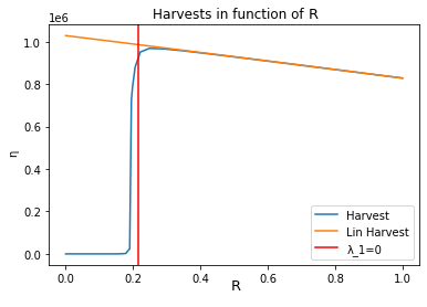
where and . We plot this function in Figure 1.
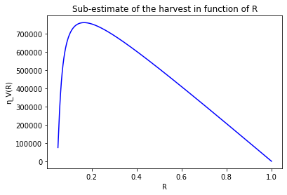
A simple computation yields the optimal of we call :
Here, .
Comment: By doing a Taylor expansion of around , one gets
which is an expression similar to that of the linearized harvest in the constant case, that will be computed later on in Remark 1.
4.1. Computation of
Let us now delve into the linearization. We suppose in the following that , the principal eigenvalue of is positive, so that converges to exponentially fast uniformly in as , as well as the exponential convergence of to (see [8]). This ensures the boundedness of , in , and the existence of .
Let us define some useful constants to lighten the writing:
-
•
,
-
•
.
We suppose in the following that is positive. This will ensure that placing refuges in the field increases , and therefore is beneficial for a quicker eradication of the population . In the case , the optimisation problem is trivial: yields the best harvest (which is in the case ).
Denote and
We have
and this quantity converges to as goes to , since . Therefore, . Similarly, and .
The population satisfies
Denote
and
We have
therefore, .
Similarly, and . The same work can be done when integrating over .
Integrating in time between and , and because ,
Integrating over ,
Because of the Neumann boundary conditions,
As a consequence,
Denote
On the other hand, using a Taylor expansion of the exponential function, the harvest verifies
where we used the boundedness of and to get .
With ,
For a test function satisfying , after integrating by part,
We now look for solutions of
supplemented with Neumann boundary conditions.
By theorem of [7] there exists a unique solution in . Denote this solution. Injecting
in the equation of the harvest, one gets
From now on, we denote
the linearized harvest.
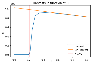
Important note: The domain of applicability for the preceding computations leading to the linearized harvest, specifically the range of parameters denoted as where is “sufficiently small”, remains uncertain. For all the results presented in this paper, we assume that encompasses the entire set of admissible parameters where is positive. This assumption is likely flawed, as we conjectured that diverges as approaches zero. We acknowledge that this assumption severs the connection between the linearized harvest and the actual harvest. Nevertheless, our results (with different boundary) should still hold within a closed, convex, and bounded set. Furthermore, we know that is not empty, as evidenced by the case where resulting in . Supposing that possesses non-empty interior within the space of all admissible parameters, then contains a closed, convex, and bounded region. We hope that the existence of this region renders the assumption more acceptable. Moreover, in numerical experiments involving a biologically consistent parameter set (details available in [8] for the sources and values of the chosen parameters), the harvest and linearized harvest are very close when is positive (even when it is small), as shown in Figure 2. This suggests that covers a significant portion of the entire set of admissible parameters within the subset where is positive. In the following sections, we look for optimizers of the linearized harvest, and we hope that the numerical simulations provided suffice to convince the relevance of studying this quantity instead of the real harvest. As seen in Figures 3 and 4, when the transmission rates are very large, the two harvests become further apart, which is consistent with the fact that becomes larger as .
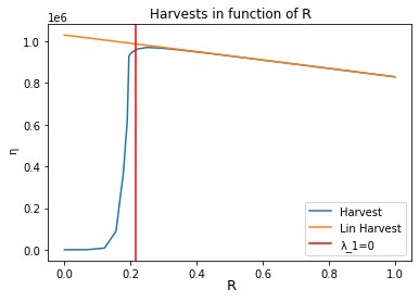
Remark 1: In figure 2, we compute the harvest and linearized harvest in the case where and are constant in space. Here, is explicit since can be computed: yields
Although it looks like a linear function of , it is not. With our parameter values (see [8] for some details), . We have taken an initial condition of one percent of the carrying capacity of .
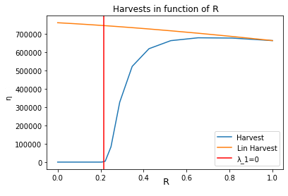
Remark 2: One can observe that the harvest is positive for some negative values of . This is, to our understanding, due to numerical imprecisions: when , while still negative, becomes very close to , diverges to much slower (at a rate that is roughly ), therefore (that we approximate by computing for a large ) becomes at a greater distance from . This phenomenon is less visible when we increase , as can be observed in Figure 5.
We denote the space of bounded functions defined on . In the proofs of Lemma 9 and Theorem 13, we use differential calculus in Banach spaces (in and in ). As the computation of the partial derivative of or with respect to is usual, we freely use it without delving into its details.
In the context of the optimization problem, the first crucial lemma is the concavity of the application :
Lemma 9.
Fix . Then, the application
is concave and coercive : .
Proof.
By the same lemma, we obtain consequently the negativity of , solving
and the positivity of in . The application is hereby concave.
The linearized harvest has the following form:
with . Hence, to prove its coercivity, it suffices to show the boundedness of when . By nonnegativity of and , is a supersolution of the Neumann system solved by , hence and the coercivity of follows.
∎
Comment: The concavity of gives interesting insights on the optimal refuge, . For instance, there exists small enough such that
is negative, and in this case . Conversely, there exists large enough such that is positive (by negativity of ), and in this case . The same comment can be made with instead of .
A natural question can arise on the convergence of the linearized harvest when the frequency of the refuge goes to infinity. We answer the question in the following proposition.
Proposition 10.
In the context of the homogenization problem (see Section 3 for the details), .
Proof.
The proof lies in the fact that .
Integrating
one gets
Multiplying the equation on by and integrating over , one gets
hence the uniform boundedness of . A direct application of the Rellich–Kondrachov theorem yields, up to extraction, the strong -convergence of to .
Let . Multiplying the equation on by and integrating over , one gets
and two integration by parts followed by passing to the limit yields
By uniqueness of the weak solution of this equation, . ∎
4.2. Schwarz rearrangement
In this section, we assume that is symmetric. In order to alleviate the proofs, we will further assume that , hence , . However, it is not, as far as we know, a necessary assumption. For an arbitrary , we will denote by the decreasing Schwarz rearrangement of , which is a symmetric, radially nonincreasing function that preserves the measures of the level sets of (see [12] and [13] for a thorough definition of the Schwarz rearrangement). With our assumptions on , also belongs in .
We call the increasing Schwarz rearrangement of , and denote , the application
Our main theorem states that, if is its own decreasing Schwarz rearrangement and is decreasing, then the optimal refuge for the linearized harvest is not constant, and there exists a refuge that is its own decreasing Schwarz rearrangement which yields a better linearized harvest than the constant refuge. The same proof also works if is its own increasing Schwarz rearrangement and is increasing, and the result would be that the optimal refuge for the linearized harvest is not constant, and there exists a refuge that is its own increasing Schwarz rearrangement which yields a better linearized harvest than the constant refuge.
Theorem 11 (Theorem 2).
Denote, for ,
.
Fix and . Let us assume that and is radially decreasing. Then,
Moreover, there exists such that and .
Proof.
Recall that
hence the quantity we aim to minimize is
with
Let . Denote and . Then, for all , . With , injecting this Taylor expansion in the equation of , one gets, at first order,
hence, dividing by and letting it go to ,
By Schwarz theorem, . Solving this ordinary differential equation with Neumann boundary conditions on with , one gets
By symmetry of and ,
Because for all , after a change of variable, one gets
and therefore, because is decreasing on ,
Moreover,
hence for a small enough , , i.e . One can easily verify that and .
∎
The next corollary is similar: if we fix the refuge , and if is its own Schwarz rearrangement, then the optimal for the linearized harvest is its own Schwarz rearrangement.
Corollary 12.
Fix .
Denote, for , . The quantities
and
exist. Moreover, if and is not constant, then
and
Proof.
With this set of constraints, one optimizes by optimizing the quantity. Let be a minimizing sequence, and be a maximizing sequence of . The set is a closed, convex and bounded subset of , therefore it is weakly compact. Hence, up to an extraction, the sequences converge to minimizing and maximizing .
Let us suppose that . By positivity of the principal eigenvalue of , the energy
is coercive, therefore is the unique minimizer of .
Moreover, by the general rearrangement inequality (see e.g Theorem 3.4 of [3]), for all and for a large constant ,
By the Pólya–Szegő inequality (see [12]), for all ,
The previous inequalities yield, for all ,
hence, by uniqueness of the minimizer of , .
Let such that Then maximizes the quantity . By the first inequality above,
By our assumption on , is increasing. By [9], . The case is treated identically, with being decreasing. ∎
4.3. Explicit optimizers in the homogeneous case
In this section, we assume that, for all , follows a given probability distribution on , such that its mean is known and homogeneous in space. Since this section is not intended to focus on probability concepts, we intentionally refrain from delving into a rigorous definition of this probability distribution. The biological rationale for this approximation is as follows: the primary provenance of aphids in the field is wind dispersal. Aphids transported by the wind cover distances significantly greater than the size of an average beet field, making it reasonable to employ a uniform mean for initially infected vectors.
The mean of the linearized harvest is
We prove in the following that the constant refuge is optimal, for the mean of the linearized harvest , in the space of bounded functions defined on we denote . Note that rather than assuming a constant mean for in space, an alternative approach is to assume itself to be constant. This would yield a similar result, asserting that a constant refuge maximizes the linearized harvest. The choice of using the mean is purely biological; it renders the assumption about the initial condition more realistic, since having constant in space appears highly unlikely in real-life scenarios.
Theorem 13 (Theorem 3).
Suppose that is constant. Let . Then
Proof.
First of all, by Lemma 9, the application is concave and coercive, which immediately yields the existence and uniqueness of the maximizer of , which nullifies .
Let so that , and let . We have
hence
Denote . There exists a sequence of step functions such that . Let be a function in .
We have shown the weak convergence in of to . By uniqueness of the limit, . By differentiating the equation on with respect to , one gets
therefore
Plugging the expression of into its equation, it yields
By uniqueness of the solution of this elliptic problem with Neumann boundary conditions (see e.g Section 3.3 of [11]), we deduce
Reciprocally, if , following the proof backwards, it is clear that . If this quantity is negative, i.e if , then a straightforward computation yields . Therefore, in this case, the optimal refuge is . ∎
Remark: We just proved that, if is constant, then . With a very similar proof, we can obtain that, if is constant, then . We deduce that, if is constant and is not constant, then is not optimal.
References
- [1] Grégoire Allaire. Lecture 1 introduction to homogenization theory, 2010.
- [2] Nikolai Bakhvalov and Grigory Panasenko. Homogenization: Averaging Processes in Periodic Media. Kluwer, 1989.
- [3] Herm Jan Brascamp, Elliott Hershel Lieb, and Joaquin Mazdak Luttinger. A general rearrangement inequality for multiple integrals. Journal of functional analysis, 1974.
- [4] Robert Stephen Cantrell, Chris Cosner, and Yuan Lou. Evolution of dispersal and the ideal free distribution. Department of Mathematics, University of Miami and Ohio State University, USA, 2010.
- [5] Edward Norman Dancer, Danielle Hilhorst, Masato Mimura, and Lambertus Peletier. Spatial segregation limit of a competition–diffusion system. Euro. Journal of Applied Mathematics, 1999.
- [6] François Murat et Luc Tartar. H-convergence. Séminaire Analyse Fonctionnelle et Numérique de l’Université d’Alger, 1977.
- [7] David Gilbarg and Neil Trudinger. Elliptic partial differential equations of second order. Springer, 2001.
- [8] Léo Girardin and Baptiste Maucourt. Agro-ecological control of a pest-host system: preventing spreading. SIAM Journal on Applied Mathematics, 2023.
- [9] Hichem Hajaiej. Cases of equality and strict inequality in the extended hardy–littlewood inequalities. The Royal Society of Edinburgh, 2004.
- [10] Juraj Húska. Harnack inequality and exponential separation for oblique derivative problems on lipschitz domains. Journal of Differential Equations, 2006.
- [11] Chia-Ven Pao. Nonlinear Parabolic and Elliptic Equations. Springer US, 1993.
- [12] Giorgio Talenti. Inequalities in rearrangement invariant function spaces. Institute of Mathematics, 1994.
- [13] Giorgio Talenti. The art of rearranging. Milan Journal of Mathematics, 2016.