TransAxx: Efficient Transformers
with Approximate Computing

Abstract

Vision Transformer (ViT) models which were recently introduced by the transformer architecture have shown to be very competitive and often become a popular alternative to Convolutional Neural Networks (CNNs). However, the high computational requirements of these models limit their practical applicability especially on low-power devices. Current state-of-the-art employs approximate multipliers to address the highly increased compute demands of DNN accelerators but no prior research has explored their use on ViT models. In this work we propose TransAxx, a framework based on the popular PyTorch library that enables fast inherent support for approximate arithmetic to seamlessly evaluate the impact of approximate computing on DNNs such as ViT models. Using TransAxx we analyze the sensitivity of transformer models on the ImageNet dataset to approximate multiplications and perform approximate-aware finetuning to regain accuracy. Furthermore, we propose a methodology to generate approximate accelerators for ViT models. Our approach uses a Monte Carlo Tree Search (MCTS) algorithm to efficiently search the space of possible configurations using a hardware-driven hand-crafted policy. Our evaluation demonstrates the efficacy of our methodology in achieving significant trade-offs between accuracy and power, resulting in substantial gains without compromising on performance.

I Introduction

Deep Learning (DL) has achieved remarkable success in a vast range of applications such as image processing, where it has emerged as one of the most powerful and accurate techniques. CNNs are capable of achieving high accuracy and performance on visual recognition and complex regression algorithms. In addition to CNNs, recent advancements in deep learning have led to the emergence of Vision Transformer (ViT) models, a new type of neural network architecture based on the self-attention mechanism of transformers which have achieved state-of-the-art performance on various computer vision tasks. However, ViT models are very computationally expensive due to their large number of parameters and the self-attention mechanism used in their architecture. Their high computational demands have limited their applicability on resource-constrained devices.

The utilization of approximate computing has demonstrated potential in enhancing the efficiency of deep learning models by reducing their computational complexity and memory demands [1]. It involves trading off a small amount of accuracy in DNNs for significant gains in speed and power efficiency by using inexact arithmetic components in place of their accurate counterparts [2, 3, 4]. Although, approximate computing has emerged as a promising approach to improve the efficiency of DNNs, no prior research has investigated its exploitation and applicability on transformers.

The wide-ranging and extensive domain of approximate compute units (ACUs) and their non trivial impact on the DNN accuracy increase the complexity of designing such hardware. Thus, the need for an approximate emulation framework that can address this intricacy becomes apparent. Moreover, as DNNs become deeper, they become more sensitive to approximation [5] and hence, approximation-aware retraining is required to recover the error introduced by approximation [5, 6, 7]. Especially, in the case of ViT models, information distortion of the self-attention map which involves a large number of operations may lead to even greater errors being introduced by lower precision [8]. In addition, determining the appropriate approximate multiplier for each DNN layer (cross-layer) is of utmost importance when targeting to maximize the power gains under accuracy loss constraints [6]. Many works have examined automated methods for determining the optimal per-layer quantization in quantized DNNs [9, 10, 11]. However, few previous works [12] have examined an automatic search flow in approximate DNNs. If ViT models were intended for use, especially for large datasets such as ImageNet, the computational cost would be tremendous, thus it would be undoubtedly a design challenge.

In this paper, we present TransAxx, a fast emulation framework of approximate multipliers in ViT models. TransAxx is developed on top of PyTorch and can run on Nvidia GPUs. The objective of TransAxx is to streamline and accelerate seamlessly, for the first time, the process of simulating popular ViT models on approximate hardware. It acts as a seamless PyTorch plugin that can be enabled by the user without obstructing the natural flow of the DL framework. This is a novel emulation platform, enabling support for the widespread PyTorch framework whose ecosystem has been known for taking over AI researchers [13]. It can efficiently handle all popular ViT models and perform approximate inference supporting mixed approximation (per-layer) as well. Additionally, a calibrated post-training quantization and approximate re-training is also supported for further accuracy improvement. Finally, we use TransAxx and present an algorithm for automatic per-layer approximation that efficiently traverses the tree of possible solutions. Specifically, we developed a Monte Carlo Tree Search (MCTS) based method (which is often used as component in RL tasks) along with a dynamic hardware-driven policy to reduce the search process. Our contributions can be summarized as follows:

1. We propose TransAxx, the first framework to seamlessly and efficiently simulate approximate ViT models.

2. We evaluate for the first time the impact of approximate multipliers on popular pre-trained ViT models on ImageNet.

3. We use an optimized post-training quantization and approximate-aware finetuning strategy to recover the accuracy loss due to approximation.

4. We propose a MCTS-based search method to flexibly balance the exploration and exploitation, while considering inference power reduction and model accuracy.

II Related Work

Taking cue from the remarkable achievements of transformer models in the domain of natural language processing (NLP), scientists have recently utilized transformer models to address computer vision (CV) challenges. However, just like CNNs, ViT models are troubled with heavy computational cost, thus applying quantization techniques, which is lowering the bit-width of the weights or activations can often address the memory requirement and computational cost of the model. Despite the recent progress made in developing quantized ViT models, approximate ViT models and their behavior remains an open issue. Also, automated mixed precision techniques for quantized CNNs have been already investigated by the community to strike a balance between the computational efficiency and the numerical stability but there is no research for approximate ViT models.

II-A Quantized ViT models

Li et al. proposed Q-ViT [8], a fully differentiable quantization technique for ViT models that focuses on a head-wise bit-width and switchable scale. Ding et al. [14] proposed APQ-ViT which introduced a unified bottom-elimination blockwise calibration scheme to surpasses the typical post-training quantization which causes significant performance drops. Last, Liu et al. [15] presented an effective post-training quantization algorithm that finds the optimal low-bit quantization intervals for weights and inputs and introduced a ranking loss to keep the relative order of the attention layer values.

II-B Approximate multipliers in CNNs

Approximate computing takes a different approach, on top of quantization, by intentionally introducing errors into computations in exchange for reduced computational cost. Several previous works have presented custom DNN frameworks to simulate the accuracy of approximate CNNs. For example, TFapprox [6] or ProxSim [16], are frameworks built on top of TensorFlow to emulate approximate circuits in CNNs using GPU accelerators. Mrazek et al. proposed ALWANN [12], a methodology to apply layer-wise approximation on 8bit ACUs with finetuning capabilities. The experimental results of these works, however, are limited mainly to ResNet CNN models for small datasets like Cifar-10. Other frameworks, such as AdaPT [17] and ApproxTrain [18] experimented on a wide range of DNNs but did not propose a design space exploration strategy while posing difficulties for the users to test their custom models.

II-C Automated Approximation frameworks

Mixed-precision quantization shows promise in providing an extra boost in speed and reducing model size by taking advantage of model redundancy and assigning lower bit-width to less sensitive or less useful layers in the model. However, the challenge lies in accurately measuring each layer’s sensitivity score and mapping it to the appropriate bit-width. A lot of techniques have been proposed such as HAWQV3 [11], a hardware-aware mixed-precision quantization formulation that uses Integer Linear Programming (ILP), or deep reinforcement learning (DRL) based quantization methods such as AutoQ [10] and HAQ [9]. While training RL agents for common hardware might be feasible, training such algorithms for simulated approximate CNNs, especially ViTs, would immensely exceed the computational and timing constraints. Approximate DNN frameworks run much slower than the default DL frameworks (i.e. [6], [12]) due to the lack of adequate support for approximate arithmetic. Additionally, the learned policies of RL agents to find optimal approximation per layer would degrade when evaluated on new ACUs or models as each ACU may behave very differently on layers with different data distributions.

III Fast Emulation of Approximate ViT Models

The TransAxx framework that we developed is intended for fast emulation of cross-layer DNN approximation and is available as a PyTorch plugin. This plugin can be activated or deactivated as desired by the user, allowing for the use of the PyTorch default flow when necessary. With TransAxx, a wide range of layer and model architectures can be seamlessly supported without any intervention by the user. Though, in this work we focus on ViT models as approximations on such models have not been investigated yet. Furthermore, we provide two key techniques for improving accuracy: post training quantization with state-of-the-art calibration and approximate-aware retraining. Additionally, TransAxx supports mixed approximation (i.e. different multipliers) in between layers. Finally, one of the primary challenges associated with using approximate components in DNNs is the need to emulate approximate operations fast, as existing DNN GPU-based accelerators do not inherently support such computations. To tackle this issue, we implement a universal GPU accelerator which can run in all Nvidia GPU architectures in order to accelerate the emulation of approximate ViT models.

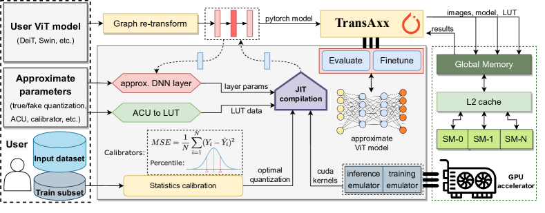
Figure 1: TransAxx framework operation

III-A Designing the framework

In order to perform computations in a DNN model which are not differentiable or rely on non-Pytorch libraries we extend the default Pytorch modules so that our functions can chain with the previous or following operations in the model. The vanilla PyTorch layers are substituted automatically by custom layers which can be instantiated using just in time (JIT) compilation on the fly (Figure 1). Regular Tensor objects perform the initialization of weights or biases and C++ macros are used to dispatch the appropriate approximate kernel for the specific input datatype (i.e. float, int8, etc.) For each approximate multiplier, a corresponding Look-up Table (LUT) is generated from its high-level description (e.g., in C, Matlab, or behavioral HDL) through TransAxx and stored in the global GPU memory which has a large size and it’s the most appropriate option for the random access patterns of our LUTs. It’s worth noticing that the cache behavior of the GPU is determined by the hardware and the memory access patterns of each ViT model but generally the LUT array will be cached through the L2 GPU cache which is a large cache that is shared between all Streaming Multiprocessors (SMs) of the GPU and eventually improves the hit rate for our LUT data. Also, in case of large bitwidth where LUTs can increase substantially TransAxx can always substitute the LUT-based multiplication with functional-based multiplication (in which the approximate multiplier is alternatively described in C-code). This approach can alleviate the problem of memory in large LUTs (>15bit) but can introduce overhead in the DNN execution time. It’s worth mentioning that both approaches provide a 1-1 representation of the multiplier at high-level thus the results would be the same in inference or retraining.

III-B Support for the transformer architecture

The transformer layer is the fundamental building block in the vision transformer architecture. Its purpose is to take a sequence of image patches as input, utilize the self-attention mechanism to establish long-range relationships, and produce a new feature sequence. There are also additional blocks at the beginning or at the end of a ViT model such as patch embedding or classification head. In patch embedding the input image is divided into fixed-size non-overlapping patches, and each patch is linearly embedded into a flat vector. These patch embeddings are then treated as the input tokens for the transformer model. At the end of the ViT model, there is typically a classification head responsible for making predictions based on the learned features. We chose to apply approximation only on the core transformer blocks involving the self-attention mechanism which largely dominate the execution time (usually $>98\%$). These blocks are often expanded to multiple transformer encoder blocks, each of which mainly contains a normalization, a multi-head self-attention, and a feed-forward layer. Towards incorporating approximate arithmetic, we will focus on the latter two which have the most mathematical operations.

The attention can be mathematically defined using the following equation, where the softmax function is used to compute the weights that determine the importance of each element in the input. Here, $Q$ is the query vector, $K$ is the key vector, and $V$ is the value vector:

$$Attention(Q,K,V)=softmax(\frac{QK^{T}}{\sqrt{d_{k}}})V$$ (1)

In short, it calculates the association between the Query vector and the Key vector and multiplies the Value associated with each Key. The division by the square root of $d_{k}$ (dimensionality of $K$ vector) is performed to maintain an appropriate variance of attention values.

Multi-head Attention Multi-head attention is a technique that uses multiple sets of (Q,K,V) triplets instead of just one set. This is done to account for cases where an element in a sequence has dependencies on more than one other elements. Using multiple weights associated with the same element provides a more comprehensive weighting of the sequence. The multi-head attention can be described as below.

$$\begin{aligned} MultiHead(Q,K,V)=Concat(head_{1},...,head_{h})W^{O}\\ \text{where}\quad head_{i}=Attention(QW^{Q}_{i},KW^{K}_{i},VW^{V}_{i}).\end{aligned}$$ (2)

Each head has its own set of learned parameters and performs the scaled dot-product attention operation separately.

Feed-Forward Network The Feed-Forward Network (FFN) is a two-layer classification network with a GELU (Gaussian Error Linear Unit) activation layer. It is designed to allow for non-linear interactions between patches or tokens in the input feature map, enabling the model to capture complex patterns and relationships. The FFN layer also involves a significant number of computations, so it is often necessary to implement approximate computing methods for this layer as well. It can be formulated as below:

$$FFN(\vec{X})=GeLU(\vec{X}W_{1}+b_{1})W_{2}+b_{2}.$$ (3)

where $W_{1}\in\mathbb{R}^{d\times d_{f}}$, $b_{1}\in\mathbb{R}^{d_{f}}$ and $W_{2}\in\mathbb{R}^{d_{f}\times d}$, $b_{2}\in\mathbb{R}^{d}$. $d_{f}$ is the inner hidden size of the Feed-Forward Network.

III-C Quantization and fine-tuning strategies

To enable approximate computing units simulation, an efficient quantization scheme that minimizes the quantization error impact must be implemented first. Note that the majority of approximate multipliers (especially for DNNs) support low bit-width integer (fixed point) arithmetic [2]. Prior work on approximate CNN simulators has mainly focused on standard 8-bit quantization [6, 16], although in TransAxx we utilize a versatile bitwidth quantizer. As our paper’s scope does not involve proposing a new quantization method, we employed a state-of-the-art open-source quantizer based on Nvidia’s TensorRT toolkit that can accommodate both lower and higher precisions. This flexibility can be crucial when simulating higher precision ACUs for deep neural networks that might lack error resilience [19, 20].

The mapping between real and quantized values must be affine, meaning they must follow the equation $Real\_Value=A\times Quantized\_Value+B$ where $A$ is the scale and $B$ is the zero point (often set to zero). To determine the most suitable quantization parameters for the scale values, we utilized a calibration technique to gather data statistics. Our quantization modules were implemented with the histogram calibrator, targeting a 99.9% percentile, as it delivered the best performance overall. However, alternative methods like MSE (Mean Squared Error) or entropy can be applied transparently in our framework if desired. Furthermore, optionally after post-training quantization, we can perform Quantization Aware Training (QAT) by continuing training the calibrated model based on Straight Through Estimator (STE) derivative approximation. Notably, in Transaxx, QAT is approximation-aware as it simulates the approximate noise of ACUs during the finetuning stage and eventually shows more robustness to the applied multipliers. During approximate-aware retraining, TransAxx propagates the computations through our ACUs (usually for 2.5% of the default training schedule) effectively computing the layer gradients using STE and increasing the final accuracy of the approximate ViT model at the end.

III-D Toy experiment

A toy experiment was conducted to test the effectiveness of backpropagation on a simple attention layer that used an 8-bit approximate multiplier instead of the default FP32 arithmetic of PyTorch. The core attention mechanism works by focusing on specific parts of the input sequence based on their relevance to the current output. The goal of this experiment is to see if a simple layer with the core attention mechanism can backpropagate correctly and ensure, thus, that its functionality is not compromised by the approximate hardware emulation.

To perform the experiment, the attention layer was modified to use a mul8s_1L2H approximate multiplier from the Evoapprox lib [21] for the forward and backward passes. The modified layer was then trained using a standard Stochastic Gradient Descent (SGD) algorithm for 500 iterations on data taken from $\mathcal{N}(0,1)$. The results presented in Figure 2 showed that backpropagation on our framework works as expected minimizing the MSE while the target values in the layer exhibit similarity with the accurate layer. Mathematically, the output data $Y$ converges in probability to the target data $X$ because as the number of samples (n) approaches infinity, the probability that the difference between $Y_{n}$ and $X$ being greater than some small value epsilon approaches zero.

$$lim_{n->\infty}P(|Y_{n}-X|>epsilon)=0.$$ (4)

Epsilon here is a threshold that specifies the maximum allowable error between the output and target values and it is ultimately dependent on the approximate multiplier used.

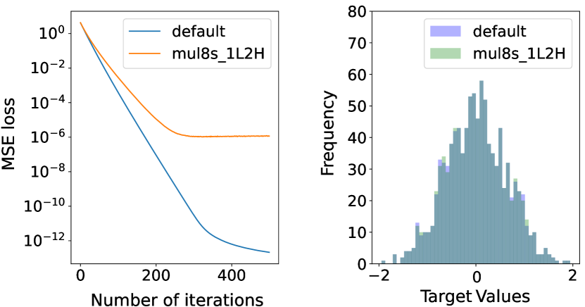
Figure 2: Left: MSE loss per iteration. Right: Histograms of target data.

IV Searching the Space of Approximate Designs

Exposing the optimal configuration of approximate multipliers between each layer of a DNN model in order to find the best trade-off between performance and power is liable to cause a significant computational overhead. The design space becomes large and measuring the accuracy of every configuration is not feasible even when using our GPU-based acceleration, particularly in our case, where the ViT simulation increases further the execution time. To efficiently explore the approximate design space we use a hardware-driven Monte Carlo tree search (MCTS) to narrow down the architecture space for the approximate ViT models, maximizing accuracy while still meeting our given power constraints. To further reduce feedback time, we also developed an accuracy predictor for the inference accuracy. Our method reaches a near Pareto-optimal curve between power and accuracy.

IV-A Rationale for employing MCTS

Monte Carlo Tree Search (MCTS) is an AI search technique, often used in board games, that uses probabilistic and heuristic-driven algorithms to combine the classic implementation of tree search with principles from machine learning and particularly reinforcement learning. MCTS has the ability to dynamically balance exploration and exploitation, making it less susceptible to getting stuck in local optima compared with other methods such as greedy algorithms which are often used for quantization precision search [22, 23]. Specifically, the case of using inexact arithmetic can introduce additional sources of error that can make the optimization problem more complex to solve as it requires a greater degree of exploration than the greedy methods.

In addition to these methods, RL agents and genetic algorithms have also been used for finding optimal hardware configurations in CNNs [9], though applying them for our case would be unrealistic. The reason over not training an RL agent is twofold. Training and converging an agent would require a lot of data which would greatly exceed the computational and timing constraints by simulating a vast number of ViT models. Also, the effectiveness of the learned policies of the agent for determining the optimal approximation per layer may deteriorate when assessed on new ACUs or models, given that different ACUs exhibit significant variability in their behavior across layers with distinct data distributions. Besides RL approaches, comparing with the use of genetic algorithms, MCTS has the potential to find a good solution faster and more reliably by balancing exploitation and exploration, which is crucial for this computationally expensive design space. Also, the effort required to optimize the parameters of the MCTS algorithm (e.g. exploration coefficient) is lower than the effort required for the genetic algorithms [24]. Thus it would be problematic to apply genetic algorithms towards this complex problem which inhibits high variability across different ACUs.

IV-B The proposed algorithm

In MCTS, nodes are the building blocks of the search tree. The high level description of our approach (also shown as pseudocode in Algorithm 1) is as follows:

1. Create a root node with an initial state of the model.

2. Traverse the tree selecting the node with the best Upper Confidence Bound (UCB) value according to (5) until a leaf node is reached.

3. If the leaf node is not terminal, expand it by creating child nodes for all possible actions from that state.

4. Simulate a rollout from the selected child node based on the input policy $P$ until a terminal state is reached. Here, we take actions by choosing a potential ACU for the layer $l_{i}$ of the ViT model (we followed a head-wise approach similar to [8]) and treat the state terminal when ${M(A_{i})}_{i=1}^{L},$ where each layer $l_{i}$ of the $L$ layers has an applied ACU $A_{i}$. Then, we compute the reward of the current approximate configuration of this rollout.

5. Backpropagate the reward obtained from the rollout up to root and update all UCB values of visited nodes.

(a) VeiT-S

(b) DeiT-S

(c) Swin-S

(d) GCViT-XXT

Figure 3: Analysis of the real (red) and predicted (blue) accuracy on per-layer approximation for various ViT models.

$$S_{i}=x_{i}+c\sqrt{\frac{\ln N_{i}}{n_{i}}},$$ (5)

where $S_{i}$ the value of node $i$, $x_{i}$ the empirical mean of node $i$, $c$ the exploration constant, $N_{i}$ the total number of simulations up to $i$ and $n_{i}$ the number of visits of the node.

The cycle of selection, expansion, simulation and backpropagation continues until it reaches the user-defined time limits. Every terminal state is expressed as $S=(A_{1},A_{2},\dots,A_{L})$ and all the environment-specific information that is relevant for the decision-making process has been included, specifically the power consumption of the current configuration and the output from the accuracy predictor. Also, the exploration-exploitation ratio can be tuned using $c$ variable from the UCB formula. The accuracy from the predictor is computed in each rollout of the MCTS tree as evaluating the real accuracy on the whole dataset (ImageNet in our case) would be impractical. Root Mean Square Error (RMSE) was used as a metric to reflect the magnitude of the error of the target models. The output was compared with the ground truth using the square root of the typical MSE formula: $\sum_{i=1}^{N}(x_{i}-y_{i})^{2}$ for $128$ input samples which was proven to suffice the majority of our scenarios. In general, determining where to allocate the right multiplier is not straightforward. The aim of MCTS is to explore alternative paths which might be perceived as sub-optimal so that the system can avoid getting stuck in local optima.

Figure 3 represents the normalized true and predicted accuracy (red and blue bars respectively) after applying the mul8s_1L2H ACU in the first 5 layers individually for every target model. Through these ablation studies we show our primary objective, which is not to achieve precise predictions of the accuracy, but rather to produce estimations that capture the general trend of the actual accuracy. Also, upon observation of the figure, it is evident that each layer block has a different sensitivity towards the perturbation of the final accuracy. This sensitivity list is beneficial for producing a better policy during the rollout phase of MCTS as we discuss next.

Defining a better policy: Rollout policy is usually a simple heuristic to estimate the reward of a given state by randomly choosing actions until the terminal state is reached [25]. It is often implemented as a random policy, where actions are selected uniformly at random without any particular strategy but with the aim to explore a wider range of states. Using domain-specific knowledge of the sensitivity of each layer to approximation, we implemented a more sophisticated policy.

Let $S=(s_{j,1},s_{j,2},\dots,s_{j,L})$ be the layer sensitivity list of an ACU $A_{j}$. $s_{j,i}$ is the normalized accuracy of the model when ACU $A_{j}$ with $j\in[1,k]$ is applied only on layer $i$. Similarly, we can represent the total returned power of the approximate model when $A_{j}$ is applied on layer $i$ as $p_{j,i}$. Conclusively, we can now express the probability of taking a specific action in the rollout policy, that is to select an $A_{j}$ out of $k$ available ACUs for layer $i$ as:

$$P(A_{j})_{i}=\frac{e^{(s_{j,i}-\lambda\times p_{j,i})}}{\sum_{z=1}^{k}e^{(s_{z,i}-\lambda\times p_{z,i})}}$$ (6)

We incorporated expert knowledge to our problem by producing a better-informed rollout taking feedback from both sensitivity and power in each layer. Although we are making assumptions based on available knowledge, we incorporated randomness into the selection as well. This approach reflects optimism in the face of uncertainty which as a mathematical concept has underpinned many decision-making algorithms [26, 27]. In our case, this policy gave consistently stronger performance than the default random heuristic.

Algorithm 1 Pseudocode for our hw-driven MCTS

Input: 1) Model $M$,   2) Ground truth batch $B_{g}$,   3) Selected ACUs $A$,
4) Exploration constant $c$,    5) Rollout policy $P$,    6) No. of Simulations $N$
Output: 1) Optimal Approx. Configs $C_{out}$

1:$rootNode\leftarrow Node(M)$

2:for $i\leftarrow 1$ to $N$ do

3:     $node\leftarrow rootNode$

4:    while not $node.isTerminal()$ do

5:        if $node.isFullyExpanded()$ then

6:            $node\leftarrow node.getBestChild(c)$

7:        else

8:            $node\leftarrow expand(node)$

9:            break

10:        end if

11:    end while

12:     $state\leftarrow node.state$

13:    while not $state.isTerminal()$ do

14:         $a\leftarrow chooseAction(state,P,A)$

15:         $state\leftarrow state.takeAction(a),a\in A$

16:    end while

17:     $Y_{i}\leftarrow AxxConfig(state)$

18:     $accuracy_{i},power_{i}\leftarrow evaluate(M,Y_{i},B_{g})$

19:     $reward\leftarrow accuracy_{i}-\lambda\times power_{i}$

20:     $backprop(node,reward)$

21:end for

22:$C_{out}\leftarrow pareto(accuracy_{i},power_{i},Y_{i}),\forall i\in[1,N]$

V Experimental Results

The experiments in this study include the performance of TransAxx framework in terms of accuracy and execution time for popular ViT models and different approximate multipliers. Furthermore, we show the effectiveness of our MCTS algorithm for optimally searching the space of approximate designs to find the best balance between accuracy and power consumption. In terms of software versions, TransAxx was built on PyTorch 1.13 with CUDA Version 11.7. Also, the hardware setup we used was a 20-core Intel Xeon Gold 5218R server with 64GB of RAM and an Nvidia Tesla V100 GPU.

TABLE I: Emulation time in TransAxx for different ViTs

DNN	FLOPs	Params	Inference (w/ func.)	Inference (w/ LUT)	Retraining (w/ LUT)
ViT-S	4.2G	22.1M	121 min	6 min	5.5 min
DeiT-S	4.2G	22.1M	122 min	6.1 min	5.8 min
Swin-S	8.5G	49.6M	242 min	13.1 min	13 min
GCViT-XXT	1.9G	12M	43.5 min	3 min	3.5 min

TABLE II: Qualitative comparison with state-of-the-art

Tool Support	TransAxx	[17]	[18]	[6]	[16]	[12]	[28]
Framework	PyTorch	PyTorch	TF	TF	TF	TF	C++
Backend	GPU	CPU	GPU	GPU	GPU	CPU	CPU
ViT model support	✓	✗	✗	✗	✗	✗	✗
Automatic ACU placement	✓	✗	✗	✗	✗	✗	✗
Quantization calibration	✓	✓	✗	✗	✗	✓	✗
HW-aware retraining	✓	✓	✓	✓	✓	✗	✓
Design space search	✓	✗	✗	✗	✗	✓	✗

V-A TransAxx performance on ViT models

Our framework was built with speed but also with flexibility in mind so that it can enable users to seamlessly test their custom ACUs fast. As aforementioned, two methods are supported during emulation; the LUT-based and the funtional-based approach. Table II shows the inference time using the two approaches as well as the retraining time for an epoch for each model. The models used for our experiments are four popular ViTs, namely ViT [29], DeiT [30], Swin [31] and GCViT [32]. All experiments are done on ImageNet2012 dataset with 128 or 64 batch size. Regarding the retraining scheme, we use Adam optimizer with a learning rate of $5e^{-5}$ for 2.5% of the ImageNet train dataset. For Table II metrics, the 8-bit mul8s_1KV9w [21] is used but the execution time is similar with any ACU of the same size. The LUT-based approach is usually not affected by the type of ACU and is significantly faster than the functional-based approach, the latter of which only serves as a back-up method in TransAxx to alleviate any unforeseen memory issues. In general, the execution times are considered acceptable and fast enough, especially when considering that there is no other alternative for approximate ViT emulation. Note also that these numbers regard the complex and large ImageNet dataset. Moreover, TransAxx is faster compared to similar frameworks that do not support ViT models though. In order to compare with prior work, we can focus our comparison on the execution time of ViT-S which is closely related to ResNet50 in terms of FLOPs (4.2G vs 3.87G). TransAxx achieves faster inference time compared with other GPU simulation frameworks such as ProxSim [16] (6min vs 107min) and ApproxTrain [18] (6min vs 10.4min). Last, it’s worth noticing Table II, which shows the robustness of TransAxx in terms of features compared with the state-of-the-art, combining all the important functionalities.

TABLE III: Accuracy and power benchmark [%] per multiplier and model

Model specifications				ACU 1: mul8s_1KV9 MRE: 0.90%, power: 0.410mW			ACU 2: mul8s_1L2H MRE: 4.41%, power: 0.301mW			ACU 3: mul8s_1L2L MRE: 12.26%, power: 0.200mW
Name	MACs approx.	FP32	8bit (calib.)	Initial	Retrained	Power $\downarrow$	Initial	Retrained	Power $\downarrow$	Initial	Retrained	Power $\downarrow$
ViT-S	98.54	74.64	71.86	34.95	67.31	3.45	1.264	66.74	28.75	0.090	0.15	52.18
DeiT-S	98.54	81.34	79.34	0.96	70.16	3.45	0.10	67.01	28.75	0.10	0.11	52.18
Swin-S	99.7	82.89	81.83	79.56	79.25	3.49	64.30	76.64	29.09	0.41	67.87	52.79
GCViT-XXT	75.5	79.72	78.91	73.50	78.346	2.64	51.56	76.93	22.03	0.26	63.01	39.98

V-B Evaluation of Approximate Multiplication for ViT Models

In this subsection we perform a systematic analysis on the top-1 accuracy achieved on ImageNet-1K dataset for each of the four aforementioned ViT models on the default FP32, 8-bit quantized, approximate and retrained versions. Apart from performing successful finetuning after approximation, we considered significantly the quantization part, as also described in paragraph III-C. In particular, prior to the approximation of the models, we performed a calibrated quantization scheme since finding a scale parameter correctly is known to have a large impact on the network’s performance[33].

Regarding the approximate multipliers used for the experiments, we chose three distinct ACUs with different Mean Relative Error (MRE) and power characteristics obtained from the open-source EvoApprox library [21], and the accurate ACU which corresponds to mul8s_1KV6. Table III summarizes our accuracy results obtained before and after retraining. Generally, we see that approximate-aware retraining reduces the accuracy gap successfully on the majority of approximate models, as the weights of the network can adapt to the distributions the ACUs represent. Additionally, we report the total MAC (multiply-and-accumulate) power reduction. Clearly the actual power reduction would be influenced by numerous factors but the reduction from MAC operations usually has a cascading effect on the total consumption. The reduction percentage is in relation to the total MACs approximated in each model in order to have more precise measurements. The baseline is the power consumption of the accurate mul8s_1KV6 multiplier (0.425mW).

V-C Exploring the design space

The manual and simple method of performing approximation, that is to apply the same multiplier to all layers in the model gave us substantial power gains with the cost of some accuracy drop as seen from Table III. However, in some cases, it is not possible to recover the large impact that approximate multiplications had on accuracy. Moreover, in many cases there might be a more power efficient solution that achieves similar accuracy. In this subsection, we conduct a comprehensive analysis of our automated search algorithm based on MCTS. The results of our automated search reveal a nuanced understanding of the trade-offs inherent in the power-accuracy space. We show that we can automatically find better solutions that are closer to the Pareto-front and thus offer better trade-off between power consumption and accuracy. For our experiment the four ACUs (mul8s_1KV9, mul8s_1L2H, mul8s_1L2L, mul8s_1KV6) are considered as possible candidates for each layer of every target model.

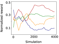
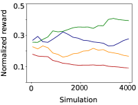
       • mul8s_1KV6   • mul8s_1KV9   • mul8s_1L2H   • mul8s_1L2L

Figure 4: Convergence of rewards on the MCTS root node for the random policy (left) and hw-driven policy (right).

Policy evaluation Before proceeding with the Monte Carlo simulations it is essential to exhibit the stability of the algorithm and its ability to converge after some iterations. Naturally, our agent’s performance is optimal when the rollout policy we used to estimate the expected rewards of each possible action is more likely to choose the best action. This is the reason we injected knowledge from the hardware configurations into the system using (6) so as to guide the search process towards the Pareto-optimal points. In Figure 4, for the case of ViT-S model, we measure the normalized reward on each simulation of the four possible starting paths/actions from the root node of the MCTS tree. In this way, we demonstrate the ability of our custom hardware-driven policy to converge to more stable rewards faster than the random policy. Another valuable insight we can obtain from this figure is that the hardware-driven policy manages to find faster what might be a good or bad action to take according to the algorithm. For example, it prefers choosing mul8s_1L2H multiplier at the first layer as it might give an ”appealing” accuracy-power tradeoff which is also indicated by our measurements in Table III. In contrary, the lower power mul8s_1L2L multiplier is not often preferred as it significantly compromises the accuracy. We should note however, that intuitively these outcomes would vary across models, layers or multipliers.

MCTS simulations: Finally, we evaluate the use of our hardware-driven MCTS algorithms towards finding the Pareto-optimal curve for accuracy and power. In Figure 5, we illustrate the scatter plots from MCTS for every target ViT model using 2000 simulations (power consumption is normalized). On average, the exploration time on most models for this setup was about $35$mins which is considered very acceptable, especially when compared with previous work [11, 12]. The user has the flexibility to tune it according to their requirements; however, further exploration yielded minimal results on the accuracy-power trade-off. Each acquired Pareto (in red) represents the knowledge learned by the system towards finding the optimal multiplier configuration and it’s basically the output of the search algorithm. To provide further comparisons, we experiment for two distinct $\lambda$ parameters for the power bias, as described in Algorithm 1 and Equation 6. For a state in the tree to be evaluated accurately, it must be visited a sufficient number of times (to gain the confidence about the statistics). Thus, the number of simulations clearly affects the quality of solutions, but we saw that around 2000 simulations were enough for most models to derive successful results in a reasonable time. Additionally, experimenting with different $\lambda$ parameters or even exploration-exploitation ratios could potentially yield marginally improved results; however, our experiments served as a strong indication of the successful application of the proposed search algorithm and parameters.

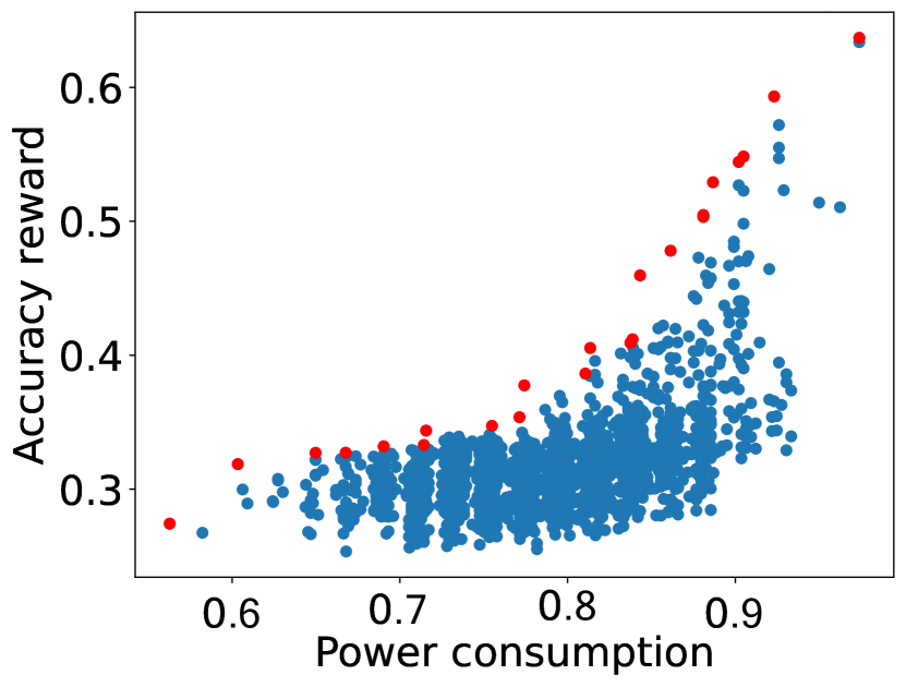
(a) ViT-S

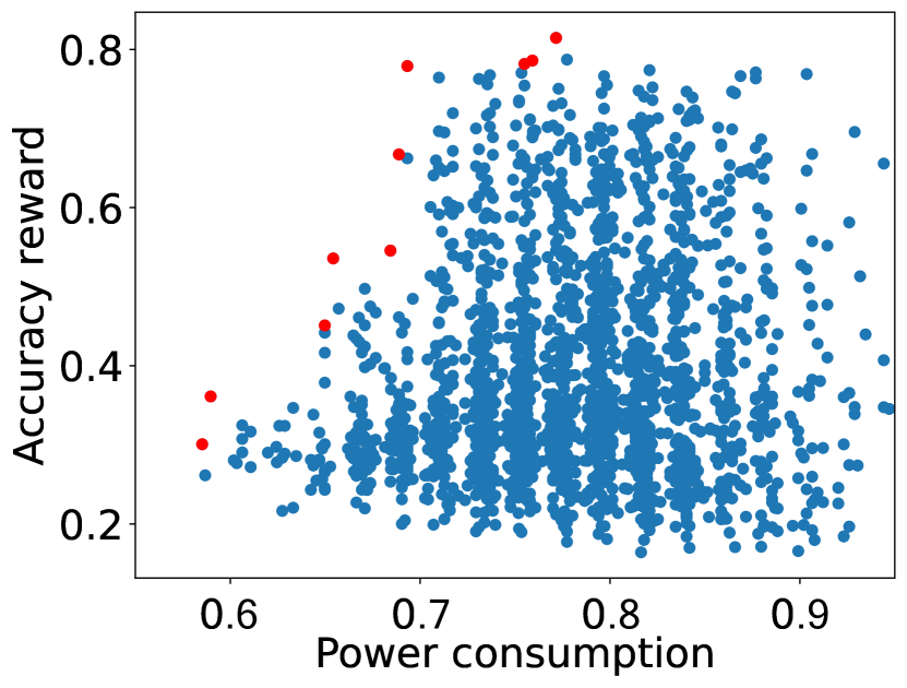
(b) DeiT-S

(c) Swin-S

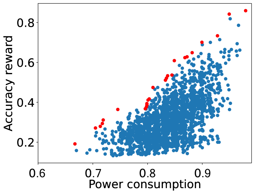
(d) GCViT-XXT

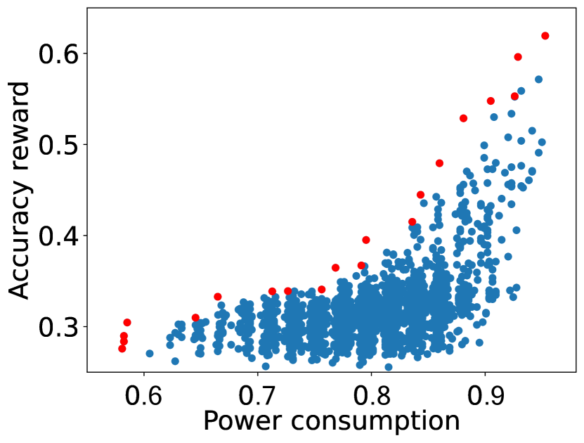
(e) ViT-S

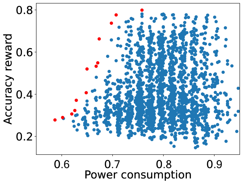
(f) DeiT-S

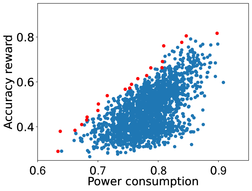
(g) Swin-S

(h) GCViT-XXT

Figure 5: Scatter plots of hw-driven MCTS using 2000 simulations for high $\lambda$ (top) and low $\lambda$ (bottom) parameter.

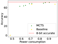
   (a) ViT-S                                      (b) DeiT-S

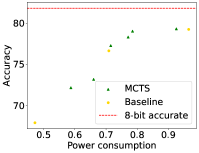
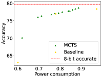
         (c) Swin-S                               (d) GCViT-XXT

Figure 6: MCTS-optimal solutions based on real accuracy (green) and baseline approximate solutions (yellow).

In Figure 6, we summarize the solutions found with the baseline approximation of the models (in yellow), obtained from Table III, along with the proposed optimal solutions obtained by our MCTS-based approach (in green). As baseline solutions we define the accuracy/power data points from Table III in which approximation is uniformly applied to all layers of the model without much customization. The corresponding scatter plots of Figure 6 illustrate the practical observation of the accuracy/power trade-off, with normalized power consumption along the x-axis and actual measured accuracy along the y axis. Notably, the study highlights the superior performance of our hardware-driven Monte Carlo tree search algorithm, particularly in achieving a more advantageous balance between power consumption and accuracy, as well as giving an increased flexibility from the designer’s perspective in choosing a wider range of accuracy-power approximate solutions.

The green data points of Figure 6 are derived from the large exploration of the parameter space using MCTS, depicted in Figure 5, focusing only on the optimal solutions achieved through this algorithm (red points in Figure 5). These data points are evaluated on the whole ImageNet validation dataset and the Pareto points are depicted in the corresponding scatter plots of Figure 6 as green triangular markers. The baseline solutions from Table III, for each approximate multiplier, are deliberately included to provide a benchmark for evaluating the effectiveness of the proposed solutions using the MCTS search algorithm.

The scatter plots of Figure 6 visually highlight the trade-offs between power consumption and accuracy. Our solutions (green points) mainly form the Pareto-front in each subplot (i.e., deliver the best best possible compromise between the two objectives, accuracy and power.) For similar accuracy as the baseline approximate solutions (within $\sim$ ​​​​​​ $1\%$ maximum difference), MCTS delivers on average solutions with $\sim\!\!\!\!\ 21\%$ lower power. Additionally, our approach yields a considerable number of Pareto solutions in all models, providing the designer with a fine-grained set of choices. These choices aim to deliver the most effective balance between the two objectives, power and accuracy, while minimizing exploration time. In contrast, the baseline approximation offers a more limited selection.

In general, our MCTS search enables obtaining results from the Pareto-curve customized to fulfill the designer’s requirements and eventually give a more fine-grained trade-off between accuracy and power with respect to the baseline approximation. Our requirements, relevant to the specific application, included constraints on power consumption, accuracy thresholds and exploration time of MCTS algorithm, but additional criteria can be involved for the system under consideration. Note that, to the best of our knowledge, our work is the first to analyze the impact of approximate multipliers on ViT models and deliver a framework for a) evaluating the inference accuracy with reasonable speed, b) performing approximation-aware ViT re-training, and c) delivering a fine-grained accuracy-power trade-off when exploring the design space of ViT to approximation mapping. Despite the considerable savings reported in Figure 6, higher power savings for similar accuracy loss have often been reported in approximate CNNs [2]. Hence, additional research is required for ViT models and/or dedicated approximate multipliers/approximation techniques are needed. Our work lays the groundwork for exploring this challenging domain and greatly facilitates designers in identifying solutions fast enough that align more closely with the desired balance of power and accuracy in ViT models.

VI Conclusion and Perspective

In this paper we introduced TransAxx, an end-to-end framework built on top of PyTorch library, that is designed for seamless and fast evaluation and re-training of approximate Vision Transformers. TransAxx is accelerated by leveraging GPU hardware without significant overhead compared with the native execution. Additionally, we introduce a novel methodology for searching the design space of approximate ViT models using a hardware-driven MCTS-based algorithm. Our findings demonstrate the capability to achieve substantial gains in both accuracy and power, specifically tailored to meet the needs and preferences of the designer, all within a short timeframe. Our work focused on primarily presenting the performance and features of our framework. Towards contributing fundamentally in the software-hardware ecosystem, TransAxx will be made available open-source.

Dimitrios Danopoulos received his diploma in Electrical and Computer Engineering from the National Technical University of Athens (NTUA) in 2018. He is currently a PhD canditate at the School of Electrical and Computer Engineering of the National Technical University of Athens. His research area involves the development and hardware acceleration of Machine Learning and Deep Learning applications. He has also contributed to various European projects by participating in the research teams.

Georgios Zervakis is an Assistant Professor at the University of Patras. Before that he was a Research Group Leader at the Chair for Embedded Systems (CES), at the Karlsruhe Institute of Technology (KIT) from 2019 to 2022. He received the Diploma and Ph.D. degrees from the School of Electrical and Computer Engineering (ECE), National Technical University of Athens (NTUA), Greece, in 2012 and 2018, respectively. Dr. Zervakis serves as a reviewer in many IEEE and ACM journals and is also a member of the technical program committee of several major design conferences. He has received one best paper nomination at DATE 2022. His main research interests include low-power design, accelerator microarchitectures, approximate computing, and machine learning.

Dimitrios Soudris received his diploma and PhD in Electrical Engineering from the University of Patras in 1987 and 1992, respectively. He worked as a Lecturer, Assistant and Associate Professor in the Department of Electrical and Computer Engineering, Democritus University of Thrace for thirteen years from 1995 until 2008. Currently, he works as a Full Professor in the School of Electrical and Computer Engineering, National Technical University of Athens. He has published more than 550 papers in international journals and conferences, holds two international patents and his research has been cited >6000 times. Also, he is the author and editor of ten books Kluwer and Springer. He is Director of Microprocessor and Digital systems Lab (MicroLab). Last, he has been project coordinator and/or and principal investigator in numerous research & development projects (>60) funded by the European Commission, ENIAC-JU, European Space Agency, the Greek Government and the European and Greek Industry.

Jörg Henkel (M’95-SM’01-F’15) is the Chair Professor for Embedded Systems at Karlsruhe Institute of Technology. Before that he was a research staff member at NEC Laboratories in Princeton, NJ. He has received six best paper awards from, among others, ICCAD, ESWeek and DATE. For two terms he served as the Editor-in-Chief for the ACM Transactions on Embedded Computing Systems. He is currently the Editor-in-Chief of the IEEE Design&Test Magazine and is/has been Associate Editor for major ACM and IEEE Journals. He has led several conferences as a General Chair incl. ICCAD, ESWeek and serves as Steering Committee chair/member for leading conferences and journals for embedded and cyber-physical systems. Prof. Henkel coordinates the DFG program SPP 1500 “Dependable Embedded Systems” and is a site coordinator of the DFG TR89 collaborative research center “Invasive Computing”. He is the chairman of the IEEE Computer Society, Germany Chapter, and a Fellow of the IEEE.

References

- [1] D. Danopoulos, C. Kachris, and D. Soudris, “Utilizing cloud fpgas towards the open neural network standard,” Sustainable Computing: Informatics and Systems, vol. 30, p. 100520, 2021.
- [2] G. Armeniakos, G. Zervakis, D. Soudris, and J. Henkel, “Hardware approximate techniques for deep neural network accelerators: A survey,” ACM Comput. Surv., vol. 55, no. 4, nov 2022. [Online]. Available: https://doi.org/10.1145/3527156
- [3] X. He, L. Ke, W. Lu, G. Yan, and X. Zhang, “Axtrain: Hardware-oriented neural network training for approximate inference,” in Proceedings of the International Symposium on Low Power Electronics and Design, ser. ISLPED ’18. New York, NY, USA: Association for Computing Machinery, 2018. [Online]. Available: https://doi.org/10.1145/3218603.3218643
- [4] D. Danopoulos, C. Kachris, and D. Soudris, “Covid4hpc: A fast and accurate solution for covid detection in the cloud using x-rays,” in Applied Reconfigurable Computing. Architectures, Tools, and Applications, S. Derrien, F. Hannig, P. C. Diniz, and D. Chillet, Eds. Cham: Springer International Publishing, 2021, pp. 327–336.
- [5] Z. G. Tasoulas, G. Zervakis, I. Anagnostopoulos, H. Amrouch, and J. Henkel, “Weight-oriented approximation for energy-efficient neural network inference accelerators,” IEEE Trans. Circuits Syst. I, Reg. Papers, vol. 67, pp. 4670–4683, 12 2020.
- [6] F. Vaverka, V. Mrazek, Z. Vasicek, and L. Sekanina, “Tfapprox: Towards a fast emulation of dnn approximate hardware accelerators on gpu,” 03 2020, pp. 294–297.
- [7] G. Zervakis, O. Spantidi, I. Anagnostopoulos, H. Amrouch, and J. Henkel, “Control variate approximation for dnn accelerators,” in 2021 58th ACM/IEEE Design Automation Conference (DAC), 2021, pp. 481–486.
- [8] Y. Li, S. Xu, B. Zhang, X. Cao, P. Gao, and G. Guo, “Q-vit: Accurate and fully quantized low-bit vision transformer,” in Advances in Neural Information Processing Systems, A. H. Oh, A. Agarwal, D. Belgrave, and K. Cho, Eds., 2022.
- [9] K. Wang, Z. Liu, Y. Lin, J. Lin, and S. Han, “Haq: Hardware-aware automated quantization with mixed precision,” in 2019 IEEE/CVF Conference on Computer Vision and Pattern Recognition (CVPR), 2019, pp. 8604–8612.
- [10] Q. Lou, F. Guo, L. Liu, M. Kim, and L. Jiang, “Autoq: Automated kernel-wise neural network quantization,” arXiv: Learning, 2019.
- [11] Z. Yao, Z. Dong, Z. Zheng, A. Gholami, J. Yu, E. Tan, L. Wang, Q. Huang, Y. Wang, M. W. Mahoney, and K. Keutzer, “Hawq-v3: Dyadic neural network quantization,” in ICML 2021, 2021. [Online]. Available: https://www.amazon.science/publications/hawq-v3-dyadic-neural-network-quantization
- [12] V. Mrazek, Z. Vasicek, L. Sekanina, M. Hanif, and M. Shafique, “Alwann: Automatic layer-wise approximation of deep neural network accelerators without retraining,” 11 2019, pp. 1–8.
- [13] N. Benaich and I. Hogarth, “State of ai report 2020,” 2020. [Online]. Available: https://www.stateof.ai/2020
- [14] Y. Ding, H. Qin, Q. Yan, Z. Chai, J. Liu, X. Wei, and X. Liu, “Towards accurate post-training quantization for vision transformer,” in Proceedings of the 30th ACM International Conference on Multimedia, ser. MM ’22. New York, NY, USA: Association for Computing Machinery, 2022, p. 5380–5388. [Online]. Available: https://doi.org/10.1145/3503161.3547826
- [15] Z. Liu, Y. Wang, K. Han, W. Zhang, S. Ma, and W. Gao, “Post-training quantization for vision transformer,” in Advances in Neural Information Processing Systems, A. Beygelzimer, Y. Dauphin, P. Liang, and J. W. Vaughan, Eds., 2021.
- [16] C. De la Parra, A. Guntoro, and A. Kumar, “Proxsim: Gpu-based simulation framework for cross-layer approximate dnn optimization,” in 2020 Design, Automation & Test in Europe Conference & Exhibition (DATE), 2020, pp. 1193–1198.
- [17] D. Danopoulos, G. Zervakis, K. Siozios, D. Soudris, and J. Henkel, “Adapt: Fast emulation of approximate dnn accelerators in pytorch,” IEEE Transactions on Computer-Aided Design of Integrated Circuits and Systems, vol. PP, pp. 1–1, 01 2022.
- [18] J. Gong, H. Saadat, H. Gamaarachchi, H. Javaid, X. S. Hu, and S. Parameswaran, “Approxtrain: Fast simulation of approximate multipliers for dnn training and inference,” IEEE Transactions on Computer-Aided Design of Integrated Circuits and Systems, pp. 1–1, 2023.
- [19] R. Krishnamoorthi, “Quantizing deep convolutional networks for efficient inference: A whitepaper,” ArXiv, vol. abs/1806.08342, 2018.
- [20] P. K. Gadosey, Y. Li, and P. T. Yamak, “On pruned, quantized and compact cnn architectures for vision applications: An empirical study,” in Int. Conf. Artificial Intelligence, Information Processing and Cloud Computing, 2019. [Online]. Available: https://doi.org/10.1145/3371425.3371481
- [21] V. Mrazek, R. Hrbacek, Z. Vasicek, and L. Sekanina, “Evoapprox8b: Library of approximate adders and multipliers for circuit design and benchmarking of approximation methods,” in Design, Automation & Test in Europe Conference & Exhibition (DATE), 2017, 2017, pp. 258–261.
- [22] C. Tang, K. Ouyang, Z. Wang, Y. Zhu, Y. Wang, W. Ji, and W. Zhu, “Mixed-precision neural network quantization via learned layer-wise importance,” 03 2022.
- [23] Y. Bengio, P. Lamblin, D. Popovici, H. Larochelle, and U. Montreal, “Greedy layer-wise training of deep networks,” vol. 19, 01 2007.
- [24] M. A. Javadi, H. Ghomashi, M. Taherinezhad, M. Nazarahari, and R. Ghasemiasl, “Comparison of monte carlo simulation and genetic algorithm in optimal wind farm layout design in manjil site based on jensen model,” in 7th Iran Wind Energy Conference (IWEC2021), 2021, pp. 1–4.
- [25] A. Uriarte and S. Ontanon, “Improving monte carlo tree search policies in starcraft via probabilistic models learned from replay data,” 01 2016.
- [26] C. Dann, T. Lattimore, and E. Brunskill, “Unifying pac and regret: Uniform pac bounds for episodic reinforcement learning,” in Proceedings of the 31st International Conference on Neural Information Processing Systems, ser. NIPS’17. Red Hook, NY, USA: Curran Associates Inc., 2017, p. 5717–5727.
- [27] E. J. Powley, D. Whitehouse, and P. I. Cowling, “Bandits all the way down: Ucb1 as a simulation policy in monte carlo tree search,” in 2013 IEEE Conference on Computational Inteligence in Games (CIG), 2013, pp. 1–8.
- [28] P. Rek and L. Sekanina, “Typecnn: Cnn development framework with flexible data types,” in Design, Automation Test in Europe Conference Exhibition, 2019, pp. 292–295.
- [29] A. Dosovitskiy, L. Beyer, A. Kolesnikov, D. Weissenborn, X. Zhai, T. Unterthiner, M. Dehghani, M. Minderer, G. Heigold, S. Gelly, J. Uszkoreit, and N. Houlsby, “An image is worth 16x16 words: Transformers for image recognition at scale,” in International Conference on Learning Representations, 2021.
- [30] H. Touvron, M. Cord, M. Douze, F. Massa, A. Sablayrolles, and H. Jegou, “Training data-efficient image transformers & distillation through attention,” in International Conference on Machine Learning, vol. 139, July 2021, pp. 10 347–10 357.
- [31] Z. Liu, Y. Lin, Y. Cao, H. Hu, Y. Wei, Z. Zhang, S. Lin, and B. Guo, “Swin transformer: Hierarchical vision transformer using shifted windows,” 2021 IEEE/CVF International Conference on Computer Vision (ICCV), pp. 9992–10 002, 2021.
- [32] A. Hatamizadeh, H. Yin, J. Kautz, and P. Molchanov, “Global context vision transformers,” arXiv preprint arXiv:2206.09959, 2022.
- [33] M. Nagel, M. Fournarakis, R. A. Amjad, Y. Bondarenko, M. van Baalen, and T. Blankevoort, “A white paper on neural network quantization,” 2021.