Conformal Predictive Programming for Chance Constrained Optimization

Abstract

Motivated by the advances in conformal prediction (CP), we propose conformal predictive programming (CPP), an approach to solve chance constrained optimization (CCO) problems, i.e., optimization problems with nonlinear constraint functions affected by arbitrary random parameters. CPP utilizes samples from these random parameters along with the quantile lemma – which is central to CP – to transform the CCO problem into a deterministic optimization problem. We then present two tractable reformulations of CPP by: (1) writing the quantile as a linear program along with its KKT conditions (CPP-KKT), and (2) using mixed integer programming (CPP-MIP). CPP comes with marginal probabilistic feasibility guarantees for the CCO problem that are conceptually different from existing approaches, e.g., the sample approximation and the scenario approach. While we explore algorithmic similarities with the sample approximation approach, we emphasize that the strength of CPP is that it can easily be extended to incorporate different variants of CP. To illustrate this, we present robust conformal predictive programming to deal with distribution shifts in the uncertain parameters of the CCO problem.

Index terms— Conformal prediction; chance constrained optimization; robust uncertainty quantification.

1 Introduction

Chance constrained optimization (CCO) problems arise in many different domains such as robot navigation [1, 2, 3], portfolio optimization [4, 5], power systems design [6, 7], and learning [8, 9]. CCO problems are of the form

$$\text{minimize }\;J(x)\;\textrm{ subject to }\;\text{Prob}(f(x,Y)\leq 0)\geq 1-\delta,$$

where $x$ is the decision variable, $J$ is a cost function, $f$ is a constraint function, $Y$ are random parameters, and $\delta$ is the maximum probability of constraint violation. The existence of chance constraints makes CCO problems hard to solve [10]. In fact, without strong assumptions on $J$, $f$, and $Y$ (e.g., $J$ and $f$ being linear and $Y$ being Gaussian), CCO problems are computationally intractable due to the need to solve multi-dimensional integrals. Even if we had the technical ability to solve such complex integrals, we usually lack information about the distribution of $Y$ which makes the integral unknown; for instance, in robotics the functions $J$ and $f$ are nonlinear and $Y$ follows an unknown distribution. A common approach is hence to sample the random parameter $Y$ and to solve an approximate optimization problem over the samples while providing probabilistic feasibility guarantees for the CCO problem. These approaches include the sample approximation approach (SAA) [11] and the scenario approach (SA) [12]. We also follow a sampling-based approach, but our algorithms and feasibility guarantees are derived through the lens of conformal prediction (CP) [13, 14].

In this paper, we propose conformal predictive programming (CPP) as a new method for solving CCO problems. CPP utilizes conformal prediction, a statistical technique that has recently gained attention as it enables efficient uncertainty quantification for predictions from machine learning models, see [15, 16]. The main idea behind CPP is to transform the CCO problem into a deterministic optimization problem by using the quantile lemma which central to the idea of CP. Using a CP argument, we can then relate the solution of this problem to the CCO problem. We make the following contributions.

• We present CPP as a new algorithm for solving general CCO problems. We present CPP-KKT and CPP-MIP as computationally tractable reformulations of CPP. We further extend CPP to deal with multiple chance constraints.

• We provide marginal probabilistic feasibility guarantees for the CCO problem which are conceptually different from feasibility guarantees provided by SA and SAA.

• To illustrate the versatility of CPP, which can seamlessly incorporate different variants of CPP, we present robust CPP that can deal with distribution shifts in $Y$.

• We illustrate the efficacy and validity of CPP on a set of case studies. While a theoretical comparison with SA and SAA is difficult, we provide a numerical comparison.

Related Work

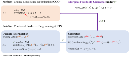
Figure 1: Conformal Predictive Programming

CCO problems have been extensively studied with early studies in [17]. Earlier works make assumptions on the distribution of the random parameter $Y$ such as being Gaussian or log-concave [18, 19, 20]. In practice, however, these assumptions usually do not hold and $Y$ is generally unknown [6]. More recent approaches do not make such limiting assumptions and solve the CCO problem approximately by sampling the random variable $Y$. We next review sampling-based approaches.

Scenario Approach (SA): Here, $K$ i.i.d. samples (or scenarios) $Y^{(1)},\ldots,Y^{(K)}$ are drawn from the distribution of $Y$, and the chance constraint is reformulated as $f(x,Y^{(i)})\leq 0,\forall i\in\{1,\ldots,K\}$ to approximate the solution to the CCO problem in (3) [21, 22, 23]. By assuming convexity of the nominal problem, the SA solution can be shown to be a feasible solution for the CCO problem with a probability of at least $1-\beta$ where $\beta$ depends on $K$ [12]. We note that these guarantees are different from the marginal probabilitistic feasibility guarantees that we derive, which do not require any convexity assumptions. Recent attempts to lift the convexity assumption are presented in [24, 25, 26, 27]. The approach with least assumptions that is most similar to our work is [23], which generates feasibility guarantees for the CCO problem using an additional dataset.

Sample Average Approximation (SAA): In SAA [11, 28], an empirical distribution from the set of sampled scenarios is used to approximate the chance constraint by instead imposing the constraint

$$\frac{1}{K}\sum_{i=1}^{K}\mathbbm{1}\{f(x,Y^{(i)})\leq 0\}\geq 1-\omega,$$ (1)

where $\omega\in(0,1)$. Feasibility guarantees of the SAA solution for the CCO problem can be obtained if the domain of $x$ is finite. In [11], under relaxed assumptions, feasibility guarantees are provided empirically with an additional dataset but without formal guarantees. We later show that CPP shares algorithmic similarities with SAA but that it allows to obtain feasibility guarantees with no assumptions on the optimization problem.

As discussed, solutions to SA and SAA reformulations are not guaranteed to be feasible for the CCO problem (3) with probability one. In robust optimization approaches [29, 30], the idea of a safe approximation allows feasibility to be preserved. A method that lies in between robust optimization and sampling-based methods is presented in [31]. To the best of our knowledge, there has been little work on bridging the gap between the optimality of solutions obtained from the approximate feasibility region (approximated using risk measures) and the feasibility region of the CCO problem. In [29], a general method for evaluating feasibility guarantees of a candidate solution $x$ to a CCO problem is proposed, arriving at similar guarantees than the scenario approach.

CCO has also been extended to solve distributionally robust CCO problems where the distribution of $Y$ is assumed to be drawn from an ambiguity set [32] constructed with moments [33, 34, 35], the Wasserstein Distance [36, 37, 38], or f-divergence [39, 40].

2 Background: Conformal Prediction

Conformal prediction (CP) is a statistical tool for uncertainty quantification that can generate probabilistically valid prediction sets for complex machine learning models, see [14, 15, 16] for an overview. Consider a set of exchangeable random variables $R,R^{(1)},\ldots,R^{(L)}$, then CP aims to find a probabilistic upper bound for $R$ based on $R^{(1)},\ldots,R^{(L)}$. In practice, $R$ can be a test datapoint while $R^{(1)},\ldots,R^{(L)}$ is a calibration dataset. The idea is now to compute the quantile over the distribution of $R^{(1)},\ldots,R^{(L)}$ at a desired confidence level $1-\delta$, which reduces to checking the rank of $R^{(1)},\ldots,R^{(L)}$. The next result summarizes the central idea behind CP where we denote by $\text{Prob}_{m}(\cdot)$ the product measure generated by $R,R^{(1)},\ldots,R^{(L)}$.

Lemma 2.1.

Quantile Lemma [Lemma 1 in [41]] Let $R,R^{(1)},\ldots,R^{(L)}$ be $L+1$ exchangeable random variables where $L\geq\lceil(L+1)(1-\delta)\rceil$. For a failure probability $\delta\in(0,1)$, it holds that

$$\text{Prob}_{m}(R\leq\text{Quantile}_{\alpha(L)}(R^{(1)},\ldots,R^{(L)}))\geq 1-\delta,$$

where $\alpha:\mathbb{N}\to[0,1]$ with $\alpha(L)\coloneqq(1+1/L)(1-\delta)$ and

$$\text{Quantile}_{\alpha(L)}(R^{(1)},\ldots,R^{(L)})\coloneqq\inf\{z\in\mathbb{R}\mid\text{Prob}_{m}(Z\leq z)\geq\alpha(L)\}$$ (2)

with $Z\coloneqq\sum_{i=1}^{L}\delta_{R^{(i)}}/L$ being a random variable with $\delta_{R^{(i)}}$ a unit point mass at $R^{(i)}$. Further, if almost surely there are no ties between $R^{(1)}\ldots,R^{(K)}$, then it holds that

$$\text{Prob}_{m}(R\!\leq\!\text{Quantile}_{\alpha(L)}(R^{(1)},\!\ldots\!,R^{(L)}))\!\leq\!1\!-\!\delta\!+\!\frac{1}{L+1}.$$

If $R^{(1)},\ldots,R^{(L)}$ are sorted in nondecreasing order, it holds that $\text{Quantile}_{\alpha(L)}(R^{(1)},\ldots,R^{(L)})=R^{(p)}$ where $p\coloneqq\lceil(L+1)(1-\delta)\rceil$, which makes it easy to compute $\text{Quantile}_{\alpha(L)}$ in practice. The variable $R$ is referred to as the nonconformity score and is often the result of a function composition, e.g., in regression a common choice is the prediction error $R:=|Z-\mu(U)|$ where a predictor $\mu$ predicts an output $Z$ from an input $U$. In this setting, we obtain the prediction region $\text{Prob}_{m}(|Z-\mu(U)|\leq C)\geq 1-\delta$ with $C\coloneqq\text{Quantile}_{\alpha(L)}(R^{(1)}\ldots R^{(L)})$. The guarantees in (2) are marginal over the randomness in $R,R^{(1)},\ldots,R^{(k)}$, as indicated by $\text{Prob}_{m}(\cdot)$. The conditional probability $\text{Prob}(R\leq C|R^{(1)},\ldots,R^{(L)})$ is known to be a random variable that follows a Beta distribution centered around $1-{\delta}$ with decreasing variance as $L$ increases, see [16] for details. We are hence inspired by the results in Lemma 2.1 in the remainder to find a solution to the CCO problem, which we formally define next.

3 Conformal Predictive Programming

Chance Constraint Optimization (CCO). Consider a probability space $(\Omega,\mathcal{F},\mathcal{P})$ with the sample space $\Omega$, the $\sigma$-algebra $\mathcal{F}$, and the probability measure $\mathcal{P}:\mathcal{F}\rightarrow[0,1]$. Let $Y:\Omega\rightarrow\mathbb{R}^{d}$ be a $d$-dimensional random vector defined over $(\Omega,\mathcal{F},\mathcal{P})$. We denote the distribution of $Y$ as $\mathcal{Y}$, i.e., $Y\sim\mathcal{Y}$. For $\delta\in(0,1)$, we define the CCO problem as

$$\min_{x}\quad J(x)$$ (3a)

s.t. $$\text{Prob}(f(x,Y)\leq 0)\geq 1-\delta,$$ (3b)

$$h_{i}(x)\leq 0,i\in\{1,\ldots,m\},$$ (3c)

$$g_{i}(x)=0,i\in\{1,\ldots,p\},$$ (3d)

where $f:\mathbb{R}^{n}\times\mathbb{R}^{d}\rightarrow\mathbb{R}$ is a measurable function defined over a decision variable $x\in\mathbb{R}^{n}$ and the random vector $Y$. We denote by $\text{Prob}(\cdot)$ the pushforward measure of $f\circ Y$, and we refer to (3b) as an individual chance constraint (or simply chance constraint). Further, let $h_{i}:\mathbb{R}^{n}\rightarrow\mathbb{R}$ and $g_{i}:\mathbb{R}^{n}\rightarrow\mathbb{R}$ denote inequality and equality constraints and $J:\mathbb{R}^{n}\rightarrow\mathbb{R}$ denote the cost function. We emphasize that $\delta\in(0,1)$ is a user-defined failure probability. We note that CPP can be extended to deal with joint chance constraints of the form $\text{Prob}(f_{i}(x,Y)\leq 0,\forall i\in\{1,\ldots,q\})\geq 1-\delta$ as we show in Appendix A, which we recommend reading after Sections 3-4. We denote the feasible region and the optimal solution of (3) as $F_{1}\subseteq\mathbb{R}^{n}$ and $x_{1}^{*}\in\mathbb{R}^{n}$, respectively. As standard in the literature, we assume that $F_{1}$ is non-empty (i.e., $x_{1}^{*}$ exists) and $J(x_{1}^{*})$ is bounded from below.
Conformal Predictive Programming (CPP). In this section, we present CPP which consists of two main steps. We first approximate the optimization problem in equation (3) by replacing the chance constraint in (3b) with a new constraint defined over the quantile in equation (2). For reasons discussed later, we then use Lemma 2.1 to conformalize the optimal solution of this optimization problem, called $x_{2}^{*}$, to certify its feasibility. Following these steps, we present two tractable reformulations of CPP in Section 4 which we call CPP-KKT and CPP-MIP. To start, we note that CPP requires two separate training and calibration datasets. We summarize our assumptions on these datasets next.

Assumption 3.1.

We have access to a training dataset of $K$ random variables $Y^{(1)},\ldots,Y^{(K)}\sim\mathcal{Y}$ where $K$ is such that $K\geq\lceil(1+K)(1-\delta)\rceil$. We further have access to a calibration dataset of $L$ random variables $Y^{(K+1)},\ldots,Y^{(K+L)}\sim\mathcal{Y}$ such that $Y,Y^{(K+1)},\ldots,Y^{(K+L)}$ are independent and where $L$ is such that $L\geq\lceil(1+L)(1-\delta)\rceil$.

Note that $Y,Y^{(K+1)},\ldots,Y^{(K+L)}$ are assumed to be independent for our main results to hold, while $Y,Y^{(1)},\ldots,Y^{(K)}$ are not required to be independent. The reason is that $f(x_{2}^{*},Y^{(1)}),\ldots,f(x_{2}^{*},Y^{(K)})$ will, for reasons we elaborate on further below, not be independent even if $Y,Y^{(1)},\ldots,Y^{(K)}$ is. However, we recommend using an independent training dataset, as we do in our experiments.
Quantile Reformulation. The motivation of our algorithm is based on Lemma 2.1. Specifically, we observe that, for a fixed parameter $x$ independent of test and training data $Y,Y^{(1)},\ldots,Y^{(K)}$, it holds that $\text{Prob}_{m}(f(x,Y)\leq\text{Quantile}_{\alpha(K)}(f(x,Y^{(1)}),\ldots,f(x,Y^{(K)}))\geq 1-\delta$ if $Y,Y^{(1)},\ldots,Y^{(K)}$ are independent. We thus approximate the optimization problem in (3) as

$$\min_{x}\quad J(x)$$ (4a)

s.t. $$\text{Quantile}_{\alpha(K)}(f(x,Y^{(1)}),\ldots,f(x,Y^{(K)}))\!\leq\!0,$$ (4b)

$$\eqref{eq:nominal_1},\eqref{eq:nominal_2}.$$ (4c)

We denote the feasible region of the optimization problem in (4) as $F_{2}(K)\subseteq\mathbb{R}^{n}$. Note that the feasible region depends on $Y^{(1)},\ldots,Y^{(K)}$, which we indicate by the input argument $K$ in $F_{2}(K)$. Due to the quantile constraint in equation (4b), it is not obvious at this point how to solve the optimization problem (4). We will defer solving this challenge to Section 4 and denote the optimal solution by $x_{2}^{*}(K)$ for now, again stressing the dependence on $Y^{(1)},\ldots,Y^{(K)}$. Note in this regard that $F_{2}(K)$ and $x_{2}^{*}(K)$ are random variables themselves given the randomness of the training dataset. For simplicity, we will often drop the dependence of $x_{2}^{*}$ on $K$.
Feasibility Guarantees. As the optimal solution $x_{2}^{*}$ depends on $Y^{(1)},\ldots,Y^{(K)}$, we note that the random variables $f(x_{2}^{*},Y),f(x_{2}^{*},Y^{(1)}),\ldots,f(x_{2}^{*},Y^{(K)})$ are no longer exchangeable. While $x_{2}^{*}$ may be a feasible solution, this loss of exchangeability means that we cannot apply Lemma 2.1 to make any formal statements about $x_{2}^{*}$. We thus conformalize the solution $x_{2}^{*}$ using the calibration dataset $Y^{(K+1)},\ldots,Y^{(K+L)}$. In essence, we perform a conformal prediction step with the nonconformity score $R^{(i)}:=f(x_{2}^{*},Y^{(i)})$ for $i\in\{K+1,\ldots,K+L\}$ and we compute

$$C(x_{2}^{*})\!\coloneqq\!\text{Quantile}_{\alpha(L)}(f(x_{2}^{*},Y^{(K+1)}),\ldots,f(x_{2}^{*},Y^{(K+L)})),$$

so that $C(x_{2}^{*})$ is a probabilistically valid upper bound on $f(x_{2}^{*},Y)$. We summarize this result in Theorem 3.2, and we provide a short proof in Appendix B.1 for completeness.

Theorem 3.2.

Feasibility of CPP Let Assumption 3.1 hold and let $x_{2}^{*}$ be the optimal solution to (4). Then,

$$\text{Prob}_{m}(f(x_{2}^{*},Y)\leq C(x_{2}^{*}))\geq 1-\delta,$$ (5a)

$$h_{i}(x_{2}^{*})\leq 0,i\in\{1,\ldots,m\},$$ (5b)

$$g_{i}(x_{2}^{*})=0,i\in\{1,\ldots,p\},$$ (5c)

i.e., equation (5) holds over the randomness in $Y,Y^{(K+1)},\ldots,Y^{(K+L)}$.

We remark that Theorem 3.2 holds in the same way for feasible (but not optimal) solutions to (4).

How do these feasibility guarantees now relate to the feasibility of the CCO problem in equation (3)? Ideally, we want that $C(x_{2}^{*})\leq 0$ in which case we expect $x_{2}^{*}$ to provide a feasible solution to the CCO problem in (3). In the way we use the quantile constraint in equation (4b) and in the way we have defined $C(x_{2}^{*})$, one can expect that the distribution of $C(x_{2}^{*})$ is centered around zero with small variance. This is confirmed by our experiments in Section 6. In practice, this hence motivates us to repeatedly draw training and calibration datasets $Y^{(1)},\ldots,Y^{(K+L)}$ and solve (4) until $C(x_{2}^{*})\leq 0$. We remark that another way of reducing $C(x_{2}^{*})$ is to enforce $\text{Quantile}_{\alpha(K)}(f(x,Y^{(1)}),\ldots,f(x,Y^{(K)}))\leq-\chi$ instead of (4b) for a tightening parameter $\chi>0$.

Finally, we would like to provide another connection to the CCO problem in (3). From equation (5a) it follows that $\text{Prob}(f(x_{2}^{*},Y)\leq C(x_{2}^{*})|Y^{(K+1)},\ldots,Y^{(K+L)})\sim\text{Beta}(L+1-l,l)$ with $l:=\lfloor(L+1)\delta\rfloor$, see [16] for details. In other words, we know that the conditional probability of $f(x_{2}^{*},Y)\leq C(x_{2}^{*})$ given the calibration dataset is Beta distributed and centered around $1-\delta$. As noted in [42], the cumulative distribution function corresponding to this Beta distribution evaluated at $1-\delta$ is $I_{1-\delta}(L+1-l,l)=1-I_{\delta}(l,L-l+1)=1-\sum_{j=l}^{L}\binom{L}{j}\delta^{j}(1-\delta)^{L-j}$ where $I_{\delta}$ is the regularized incomplete beta function evaluated at $\delta$. This implies that

$$\text{Prob}(f(x_{2}^{*},Y)\!\leq\!C(x_{2}^{*}))\!\geq\!1\!-\!\delta$$

holds with a probability of at least $\sum_{j=l}^{L}\binom{L}{j}\delta^{j}(1\!-\!\delta)^{L\!-\!j}$ over the randomness in $Y^{(K+1)},\ldots,Y^{(K+L)}$.

4 Computational Encodings of the Quantile

We next present two approaches through which the quantile in equation (4b) can be computed efficiently. The first approach is based on representing the quantile within the optimization problem (4) as a linear optimization problem. This leads to a bilevel optimization problem in which we rewrite the inner optimization problem with its KKT conditions. We call this approach CPP-KKT and show that a feasible solution to CPP-KKT is also a feasible solution to (4), but not vice versa. Our second approach, which is an equivalent reformulation, is based on mixed-integer programming (MIP) and called CPP-MIP. The idea is to reformulate the quantile within the optimization problem (4) with a set of mixed integer constraints. A feasible solution to CPP-MIP is also a feasible solution to (4), and vice versa.
Quantile Encoding and Bilevel Optimization. Following ideas presented [43, 44], we first rewrite the quantile in equation (4b) for a fixed $x$ by the linear program

$$q^{*}=\operatorname*{arg\,min}_{q}\sum_{i=1}^{K}(\alpha e^{+}_{i}+(1-\alpha)e^{-}_{i})$$ (6a)

$$\textrm{s.t. }e^{+}_{i}-e^{-}_{i}=f(x,Y^{(i)})-q,$$ (6b)

$$\quad\ \ \,e^{-}_{i},e^{+}_{i}\geq 0,\forall i\in\{1,\ldots,K\},$$ (6c)

where $q,e_{i}^{+},e_{i}^{-}\in\mathbb{R}$ are decision variables and where we use $\alpha$ instead of $\alpha(K)$ for simplicity. Intuitively, the optimization problem in (6) minimizes a weighted sum of the distance between the $\alpha$ quantile $q$ and each sample $f(x,Y^{(1)}),\ldots,f(x,Y^{(K)})$. Before we continue, we show how $q^{*}$ is related to (4b) in Lemma 4.1, with the proof provided in Appendix B.2

Lemma 4.1.

The solution $q^{*}$ to (6) upper bounds the quantile in equation (4b), i.e., it holds that $\text{Quantile}_{\alpha}(f(x,Y^{(1)}),\ldots,f(x,Y^{(K)}))\leq q^{*}$.

As shown in Appendix B.2, the upper bound $q^{*}$ is in general not conservative and exact when $\alpha K\notin\mathbb{N}$. We can now use the linear program in (6) to replace equation (4b), which results in the following optimization problem

$$\min_{x}\quad J(x)$$ (7a)

s.t. $$q^{*}\leq 0,$$ (7b)

$$\eqref{eq:nominal_1},\eqref{eq:nominal_2},$$ (7c)

$$q^{*}=\operatorname*{arg\,min}_{q}\sum_{i=1}^{K}(\alpha e^{+}_{i}+(1-\alpha)e^{-}_{i}),$$ (7d)

$$\textrm{s.t. }\ e^{+}_{i}-e^{-}_{i}=f(x,Y^{(i)})-q,$$ (7e)

$$\quad\ \ \ \,e^{-}_{i},e^{+}_{i}\geq 0,\forall i\in\{1,\ldots,K\}.$$ (7f)

Using Lemma 4.1, we immediately see that a feasible solution to (7) is necessarily a feasible solution to (4).

Corollary 4.2.

A feasible solution of the optimization problem in (7) is a feasible solution of the optimization problem (4).

Note that the inner optimization problem in equation (7) is composed of equations (7d), (7e), and (7f). For any fixed value of the decision variable $x$ from the outer optimization problem, the inner optimization problem is linear in $q,e^{+},\text{ and }e^{-}$. We can hence rewrite the inner optimization problem with its KKT conditions [45]. This results in the optimization problem

$$\min_{x,\gamma,\lambda,\beta,q,e^{-},e^{+}}\quad J(x)$$ (8a)

s.t. $$\qquad q\leq 0,$$ (8b)

$$\quad\eqref{eq:nominal_1},\eqref{eq:nominal_2},$$ (8c)

$$\quad\alpha+\gamma_{i}-\lambda_{i}=0,i\in\{1,\ldots,K\},$$ (8d)

$$\quad 1-\alpha-\gamma_{i}-\beta_{i}=0,i\in\{1,\ldots,K\},$$ (8e)

$$\quad\sum_{i=1}^{K}\gamma_{i}=0,$$ (8f)

$$\quad e^{+}_{i}\!-\!e^{-}_{i}\!-\!f(x,Y^{(i)})\!+\!q\!=\!0,i\!\in\!\{1,\ldots,K\},$$ (8g)

$$\quad e^{-}_{i},e^{+}_{i}\geq 0,i\in\{1,\ldots,K\},$$ (8h)

$$\quad\lambda_{i},\beta_{i}\geq 0,i\in\{1,\ldots,K\},$$ (8i)

$$\quad\lambda_{i}e_{i}^{+}=0,i\in\{1,\ldots,K\},$$ (8j)

$$\quad\beta_{i}e_{i}^{-}=0,i\in\{1,\ldots,K\},$$ (8k)

where $\beta_{i},\gamma_{i},\lambda_{i}\in\mathbb{R}$ are new decision variables. Specifically, (8b)-(8c) denote constraints from the outer optimization problem, while (8d)-(8f) represent the stationarity condition, (8g)-(8h) denote primal feasibility conditions, (8i) denotes dual feasibility condition, and (8j)-(8k) denote complementary slackness condition. We summarize our main result next and provide a proof in Appendix B.3.

Theorem 4.3.

The optimization problem in (8) is equivalent to (7). A feasible solution to (8) is a feasible solution to (4).

An optimal solution to (8) is a feasible solution to (4), but not necessarily its optimal solution $x_{2}^{*}$. However, we expect this optimal solution to be close to $x_{2}^{*}$ (see Lemma 4.1).

Note that (8) is a nonconvex optimization problem even when $J$, $h_{i}$, $g_{i}$ are convex and $f$ is an affine function due to constraints (8j) and (8k). However, in this case (8) is a linear complimentarity program, efficient solvers exist [46]. We next propose an alternative approach to exactly reformulate the quantile in equation (4b). We empirically compare the approaches in Section 6.
Quantile Encoding with Mixed Integer Programming. We rewrite the quantile in equation (4b) using mixed integer programming (MIP). First recall from Section 2 that $\text{Quantile}_{\alpha}(R^{(1)},\ldots,R^{(K)})=R^{(p)}$ where $p\coloneqq\lceil(K+1)(1-\delta)\rceil$ when $R^{(1)},\ldots,R^{(K)}$ are sorted in non-decreasing order. Note hence that the quantile constraint in (4b) requires that at least $\lceil(K+1)(1-\delta)\rceil$ out of the $K$ constraints $f(x,Y^{(i)})$ are satisfied, i.e., that

$$\sum_{i=1}^{K}\mathbbm{1}\{f(x,Y^{(i)})\leq 0\}\geq\lceil(K+1)(1-\delta)\rceil,$$ (9)

where $\mathbbm{1}\{\cdot\}$ is the indicator function. We proceed by introducing binary variables $z_{i}\in\{0,1\}$ for $i\in\{1,\dots,K\}$ that encode the satisfaction of $f(x,Y^{(i)})\leq 0$ along with a set of mixed integer linear constraints. Specifically, let

$$f(x,Y^{(i)})\leq M(1-z_{i}),i\in\{1,\dots,K\},$$ (10a)

$$f(x,Y^{(i)})\geq\zeta+(m-\zeta)z_{i},i\in\{1,\dots,K\},$$ (10b)

where $\zeta\in\mathbb{R}$ is a small positive constant, e.g., machine precision, and $M\in\mathbb{R}$ and $m\in\mathbb{R}$ are sufficiently large positive and small negative constants, respectively (details below). The constraints in (10) enforce that $z_{i}=1$ if and only if $f(x,Y^{(i)})\leq 0$, see [47] for details. By replacing the quantile in (4b) with the set of mixed integer linear constraints in (10) we obtain

$$\min_{x,z}\quad J(x)$$ (11a)

s.t. $$\quad f(x,Y^{(i)})\leq M(1-z_{i}),i\in\{1,\dots,K\},$$ (11b)

$$\quad f(x,Y^{(i)})\geq\zeta+(m-\zeta)z_{i},i\in\{1,\dots,K\},$$ (11c)

$$\quad\sum_{i=1}^{K}z_{i}\geq\lceil(K+1)(1-\delta)\rceil,$$ (11d)

$$\quad\eqref{eq:nominal_1},\eqref{eq:nominal_2},$$ (11e)

where $M=\max_{x\in\mathcal{X}}\{f(x,Y^{(1)}),\dots,f(x,Y^{(K)})\}$, $m=\min_{x\in\mathcal{X}}\{f(x,Y^{(1)}),\dots,f(x,Y^{(K)})\}$, and $\mathcal{X}\coloneqq\{x\in\mathbb{R}^{n}\mid\eqref{eq:nominal_1},\eqref{eq:nominal_2}\ \text{are satisfied}\}$. Note that an over(under)-estimate of $M(m)$ suffices for our purpose [47], and $M$ and $m$ exist when $f$ is continuous and $\mathcal{X}$ is a compact set. The next result establishes the equivalence between the optimization problems in equations (4) and (11). It follows immediately from the previous construction and is provided without proof.

Theorem 4.4.

The optimization problem in (11) is equivalent to (4).

Solving MIP problems is in general NP-hard, which makes solving (11) NP-hard. However, these problems can usually be solved efficiently in practice, e.g., using optimization solvers such as SCIP [48], rarely encountering the worst case complexity, as we demonstrate in Section 6. Note also that the optimization problem in (11) reduces to a mixed integer linear program when $J$, $f$, $h_{i}$, and $g_{i}$ are affine functions.

Remark 1.

SAA and CPP-MIP (and thus CPP) share algorithmic similarities for the special choice of $\omega:=1-\frac{\lceil(K+1)(1-\delta)\rceil}{K}$ in equation (1) which makes equation (1) equivalent to equation (9). While this observation is intuitive, we arrived at this conclusion from independent starting points. To the best of our knowledge, unlike in [11] and other SAA variants, we need to make no assumptions on the form of the CCO problem in (3) to obtain the feasibility results in Theorem 3.2. We also emphasize that CPP provides marginal probabilistic feasibility guarantees as opposed to SA and SAA.

5 Robust Conformal Predictive Programming

CP has been an active research area over the last years with developments in adaptive CP [49, 50], robust CP [51, 52], conformalized quantile regression [53, 54], outlier detection [55, 56], and many more. We believe that the strength of our approach is that CPP can easily be extended to incorporate different versions and extensions of CP. To illustrate this point, we present robust conformal predictive programming (RCPP) in this section.

RCPP can deal with distribution shifts in $\mathcal{Y}$, i.e., when the datapoint $Y$ is not following the distribution $\mathcal{Y}$ where the training and calibration datasets are drawn from. This may be the case when training and deployment conditions are different and when there is a sim2real gap. RCPP is based on robust conformal prediction as presented in [51], which we summarize in Appendix C. It is assumed that $Y$ instead follows a distribution from the ambiguity set $\mathcal{P}(\mathcal{Y},\epsilon)\coloneqq\{\mathcal{\tilde{Y}}\mid D_{\phi}(\mathcal{\tilde{Y}},\mathcal{Y})\leq\epsilon\}$ where $\epsilon>0$ denotes the size of the distribution shift and $D_{\phi}$ is an f-divergence measure. In essence, robust CP follows the same procedure as CP but it uses a modified failure probability of $\tilde{\delta}(K)$ (see Lemma C.1 in Appendix C) which is such that $\tilde{\delta}(K)<\delta$.
Robust Conformal Predictive Programming (RCPP). We demonstrate the use of robust CP in solving robust chance constraint optimization (RCCO) problems of the form

$$\min_{x}\quad J(x)$$ (12a)

s.t. $$\quad\inf_{Y\sim\mathcal{Y}^{\prime}\in\mathcal{P}(\mathcal{Y},\epsilon)}\text{Prob}(f(x,Y)\leq 0)\geq 1-\delta,$$ (12b)

$$\quad\eqref{eq:nominal_1},\eqref{eq:nominal_2}.$$ (12c)

The difference between the RCCO in (12) and the CCO in (3) is that $Y$ is no longer drawn from the distribution $\mathcal{Y}$, but is instead drawn from a distribution $\mathcal{Y}^{\prime}$ within the ambiguity set $\mathcal{P}(\mathcal{Y},\epsilon)$. Our robust extension of CPP to solve the RCCO uses robust CP and requires the next assumption.

Assumption 5.1.

We make the same assumptions on training and calibration datasets as in Assumption 3.1, but require now that $K\geq\Big{\lceil}\frac{v^{-1}(1-\delta)}{1-v^{-1}(1-\delta)}\Big{\rceil}$ and $L\geq\Big{\lceil}\frac{v^{-1}(1-\delta)}{1-v^{-1}(1-\delta)}\Big{\rceil}$.

Note here that $v^{-1}(\cdot)$ is defined in Lemma C.1 and can be obtained by solving a set of convex optimization programs. Similar to CPP, RCPP consists of a quantile reformulation and a feasibility analysis. We summarize RCPP and its guarantees next and provide a proof in Appendix B.4.

Theorem 5.2.

Let Assumption 5.1 hold and let $x_{2}^{*}$ be the optimal solution to (4) but with $\tilde{\alpha}(K):=1-\tilde{\delta}(K)$ instead of $\alpha(K)$. Then,

$$\inf_{Y\sim\mathcal{Y}^{\prime}\in\mathcal{P}(\mathcal{Y},\epsilon)}\text{Prob}_{m}(f(x_{2}^{*},Y)\leq\tilde{C}(x_{2}^{*}))\geq 1-\delta,$$ (13a)

$$h_{i}(x_{2}^{*})\leq 0,i\in\{1,\ldots,m\},$$ (13b)

$$g_{i}(x_{2}^{*})=0,i\in\{1,\ldots,p\},$$ (13c)

where $\tilde{C}(x_{2}^{*})\!\!\coloneqq\!\text{Quantile}_{\tilde{\alpha}(L)}(f(x_{2}^{*},Y^{(K+1)}),\!\ldots\!,f(x_{2}^{*},Y^{(K+L)}))$, i.e., (13) holds over the randomness of $Y^{(K+1)},\ldots,Y^{(K+L)}$.

As in CPP, the quantile can be encoded by either a bilevel program with the KKT conditions, with $\alpha$ replaced with $\tilde{\alpha}(L)$, or by MIP as illustrated in Section 4, where $\lceil(K+1)(1-\delta)\rceil$ from (11d) is replaced with $\lceil K(1-\tilde{\delta}(K))\rceil$.

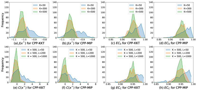
Figure 2: Results for the Numerical Example

6 Numerical Experiments

In this section, we validate CPP on a general nonlinear CCO problem and an optimal control problem. We then validate RCCP on a portfolio optimization problem. We further compare CPP with SA and SAA in Appendix D.2 and provide results for CCO problems with joint chance constraints in Appendix D.5. All experiments are conducted in Python 3 on a MacBook Air (2022) with M2 and 16GB memory using SCIP as an optimization solver.
Experimental Procedure. Our experimental evaluation proceeds in two steps. In the first step, we validate the solution $x_{2}^{*}$ of the CPP-KKT formulation in (8) and the CPP-MIP formulation in (11). Let $N$ denote the number of experiments, $K$ and $L$ again denote the size of the training and calibration sets, and $V$ denote the size of an additional test dataset. Specifically, we perform the following procedure for CPP-KKT and CPP-MIP. For each experiment $j\in\{1,\ldots,N\}$, we sample a training dataset $Y^{(1)}_{j},\ldots,Y^{(K)}_{j}\sim\mathcal{Y}$ where $\mathcal{Y}$ is problem specific. We then compute the solution $x^{*}_{2,j}$ of (8) (or (11)) and evaluate the optimal value $J(x^{*}_{2,j})$. We set a time limit of $100$ seconds for the computation of $x^{*}_{2,j}$ and report the number of timeouts in the appendix. For each solution $x_{2,j}^{*}$, we sample a test dataset $Y^{(K+1)}_{j},\ldots,Y^{(K+V)}_{j}\sim\mathcal{Y}$ and compute the empirical coverage

$$EC_{0,j}\coloneqq\frac{\sum_{i=K+1}^{K+V}\mathbbm{1}(f(x^{*}_{2,j},Y^{(i)}_{j})\leq 0)}{V}$$

to evaluate how well the CCO problem in (3) is solved.

In the second step, we validate the feasibility guarantees of CPP. Specifically, we perform the following procedure for CPP-KKT and CPP-MIP. For each experiment $j\in\{1,\ldots,N\}$, we sample a calibration dataset $Y^{(K+V+1)}_{j},\ldots,Y^{(K+V+L)}_{j}\sim\mathcal{Y}$. We then compute the upper bound $C(x^{*}_{2,j})$ to validate the feasibility guarantees in Theorem 3.2. Using the test dataset $\{Y^{(K+1)}_{j},\ldots,Y^{(K+V)}_{j}\}$, we compute

$$EC_{C,j}\coloneqq\frac{\sum_{i=K+1}^{K+V}\mathbbm{1}(f(x^{*}_{2,j},Y^{(i)}_{j})\leq C(x^{*}_{2,j}))}{V}$$

to evaluate the feasibility guarantees in Theorem 3.2. We will provide plots of the histograms of $EC_{0,j}$ and $EC_{C,j}$.

6.1 Case Study 1: General Nonlinear CCO Problem

Problem Statement. We consider the CCO problem

$$\min_{x\in\mathbb{R}} x^{3}e^{x}$$ (14)

s.t. $$\text{Prob}(50Ye^{x}-5\leq 0)\geq 1-\delta,$$

$$x^{3}+20\leq 0$$

with failure probability $\delta\coloneqq 0.05$ and where $Y\sim\text{Exp}(\frac{1}{3})$ is a long-tailed exponential distribution.
Results. For now, we fix $N\coloneqq 300$ and $V\coloneqq 1000$. In the first validation step, we vary the value of $K\in\{50,300,500\}$. We show the empirical distributions of $J(x_{2,j}^{*})$ for CPP-KKT in Figure 2(a) and for CPP-MIP in Figure 2(b). In both cases, we see that the distributions of the cost $J(x_{2,j}^{*})$ has decreasing variance for larger values of $K$, and that the distribution $J(x_{2,j}^{*})$ for $K\in\{300,500\}$ is centered at approximately $-1$, while the center of $J(x_{2,j}^{*})$ for $K=50$ is slightly bigger. Intuitively, this makes sense since more training data is expected to increase the optimality of the solution and to decrease the variance. We next show the empirical distribution of $EV_{0,j}$ for CPP-KKT in Figure 2(c) and for CPP-MIP in Figure 2(d). Both distributions are centered at $0.95$ with decreasing variance for larger values of $K$. For the value of $\delta=0.05$, this is exactly the behavior that we expect and would like to see. In the second validation step, we fix $K:=500$ and vary the value of $L\in\{50,200,1000\}$. We show the empirical distributions of $C(x_{2,j}^{*})$ for CPP-KKT in Figure 2(f) and for CPP-MIP in Figure 2(g). Both distributions are centered at $0$ (as we argued before) with decreasing variance as we increase $L$. We next plot the distributions of the empirical coverage $EV_{C,j}$ for CPP-KKT in Figure 2(g) and for CPP-MIP in Figure 2(h). Again, these are centered at $0.95$ with decreasing variance as $L$ increases, confirming our theoretical results in Theorem 3.2. We provide additional experimental results for different values of $K$ and $L$ in Appendix D.1. There, we also provide a table where we record the average statistics attained with varying $K$ and $L$ including the solver time for CPP-KKT and CPP-MIP in Table LABEL:table:average_statistics. We observe that CPP-MIP is faster on average than CPP-KKT, and no timeout nor infeasible solution was observed in Case Study 1. We compare CPP to SA and SAA in this setting in Appendix D.2.

6.2 Case Study 2: Optimal Control Problem

Problem Statement. We demonstrate the effectiveness and utility of the CPP algorithm in solving a stochastic optimal control problem. Consider a robot operating in a two-dimensional Euclidean space, e.g, a mobile service robot. The state of the robot is $y_{t}\coloneqq[x^{(1)}_{t},v^{(1)}_{t},x^{(2)}_{t},v^{(2)}_{t}]\in\mathbb{R}^{4}$ where $x^{(1)}_{t},v^{(1)}_{t}$ and $x^{(2)}_{t},v^{(2)}_{t}$ represent position and velocity at time $t$ in each dimension. We describe the robot dynamics by discrete-time double integrator dynamics

$$y_{t+1}=Ay_{t}+Bu_{t}+w_{t},\;y_{0}:=(0,0,0,0)^{T}$$

with $A\coloneqq\begin{bmatrix}1&1&0&0\\ 0&1&0&0\\ 0&0&1&1\\ 0&0&0&1\end{bmatrix}$, $B\coloneqq\begin{bmatrix}0.5&0\\ 1&0\\ 0&0.5\\ 0&1\end{bmatrix}$ and where $u_{t}\in\mathbb{R}^{2}$ is the control input and $w_{t}\in\mathbb{R}^{4}$ is system noise. Specifically, in this setting we let each entry of $w_{t}$ be drawn from a Laplace Distribution, $\text{Laplace}(0,0.02)$, and we let $T\coloneqq 5$ to be a user-specified time horizon.

We are interested in synthesizing control inputs $u_{t}$ for times $t=0,\ldots,T-1$ that allow the robot to reach a region centered around the target location $[z^{(1)},z^{(2)}]\coloneqq[5,5]$ at time $T$ with high probability. Specifically, for parameters $\delta\coloneqq 0.1$ and $\zeta\coloneqq 1$, we want to solve the control problem

$$\min_{u}\quad\sum_{t=0}^{T}\|u_{t}\|_{2}^{2}$$ (15)

s.t. $$\quad\text{Prob}((x_{T}^{(1)}-z^{(1)})^{2}+(x_{T}^{(2)}-z^{(2)})^{2}\leq\zeta)\geq 1-\delta,$$

$$\quad y_{0}=(0,0,0,0)^{T},$$

$$\quad y_{t+1}=Ay_{t}+Bu_{t}+w_{t},\forall t\in\{1,\ldots,T-1\}$$

Results. We repeat the experimental procedure as previously outlined, but now with fixed parameters $N\coloneqq 100$, $V\coloneqq 1000$, $K\coloneqq 70$, and $L\coloneqq 200$. We perform the same validation as in Case Study 1 and we report the same plots for CPP-KKT and CPP-MIP in Figure 6 in Appendix D.3. We observe the same pattern as before and specifically note that CPP provides the desired coverage of $90$ %. It is also worth mentioning that, in this case study, CPP-KKT outperforms CPP-MIP in terms of solve time, which is 5.15 seconds and 16.75 seconds on average, respectively. We postulate that, in this case study, the NP-hardness of the MIP solver plays a role so that the solver has to branch more in the solve tree while KKT conditions appear more efficient.

6.3 Case Study 3: Portfolio Optimization Problem

In this case study, we demonstrate RCPP in solving a RCCO problem in the setting of portfolio optimization. We specifically compare RCPP to CPP as a baseline model.
Problem Statement. We consider an investment portfolio optimization problem consisting of three assets. The weight of each assets (i.e., our investment) in the portfolio is represented by the vector $x\coloneqq[x_{1},x_{2},x_{3}]\in\mathbb{R}^{3}$ where each asset should be larger than the minimum permissible asset $w_{min}\in\mathbb{R}$ and the total investment should be constrained by a limit $w_{total}$. The return rate of each of the three assets, denoted by the vector $Y$, are assumed to follow a normal distribution. Specifically, we describe the distribution from which we draw training and calibration datasets as $\mathcal{Y}\coloneqq[\mathcal{N}(0.12,0.013),\mathcal{N}(0.1,0.01),\mathcal{N}(0.07,0.008)]$. The test data $Y$ is drawn from the distribution $\tilde{\mathcal{Y}}\coloneqq[\mathcal{N}(0.1,0.013),\mathcal{N}(0.11,0.011),\mathcal{N}(0.07,0.007)]$ which simulates a distribution shift from $\mathcal{Y}$. We explain how we calculate the size of the distribution shift $\epsilon$ in Appendix D.4. The inter-asset risk association is captured by a risk weight matrix $T$, and the portfolio’s overall risk tolerance is quantified by a threshold $\eta$. Additionally, this problem includes a chance constraint, ensuring that the portfolio’s return exceeds a lower-bound $\theta$ with high probability. The objective of this problem is to maximize $\theta$. Specifically, we want to solve the CCO problem

$$\max_{x} \qquad\theta$$ (16)

s.t. $$\qquad\text{Prob}(x^{\top}Y\geq\theta)\geq 1-\delta,$$

$$\qquad x^{\top}Tx\leq\eta,$$

$$\qquad\sum x_{i}\leq w_{total},$$

$$\qquad\theta\geq 0,$$

$$\qquad x_{i}\geq w_{min},i=1,2,3,$$

where $\delta\coloneqq 0.2$, $w_{total}\coloneqq 100$, $w_{min}\coloneqq 10$, $T\coloneqq\begin{bmatrix}0.06&0.07&0.02\\ 0.09&0.05&0.03\\ 0.03&0.02&0.01\end{bmatrix}$, and $\eta:=350$.
Results. We again follow the experimental procedure outlined before. However, we now apply CPP and RCPP each with the KKT and the MIP variants with parameters $N\coloneqq 100$, $V\coloneqq 1000$, $K\coloneqq 80$, and $L\coloneqq 200$. We show the results in Fig. 7 in Appendix D.4. In summary, we observe that RCPP (both with KKT and MIP) achieve the desired coverage of $80$ % while CPP (both with KKT and MIP) achieves a lower coverage as it does not account for the distribution shift between $\mathcal{Y}$ and $\tilde{\mathcal{Y}}$.

7 Conclusion

We presented CPP as a new algorithm for solving general CCO problems. CPP is based on the quantile lemma from conformal prediction which allows us to provide marginal probabilistic feasibility guarantee for the CCO problem. We also presented two tractable reformulations and extended CPP to deal with multiple chance constraints and distribution shifts. We experimentally evaluated our method on three extensive case studies. For future work, we will analyze probabilistic optimality of CPP, and we will focus on exploring theoretical connections with other sampling-based approaches such as SA and SAA.

8 Acknowledgements

The National Science Foundation supported this work through the following grants: CAREER award (SHF-2048094), CNS-1932620, CNS-2039087, FMitF-1837131, CCF-SHF-1932620, the Airbus Institute for Engineering Research, and the funding by Toyota R&D and Siemens Corporate Research through the USC Center for Autonomy and AI.

Appendix

Appendix A Conformal Predictive Programming for Joint Chance Constrained Optimization

In practice, we often require the simultaneous satisfaction of multiple chance constraints with high probability. Specifically, in such cases, we are interested in solving the optimization problem

$$\min_{x}\quad J(x)$$ (17a)

s.t. $$\text{Prob}(f_{j}(x,Y)\leq 0,\forall j\in\{1,\ldots,s\})\geq 1-\delta,$$ (17b)

$$h_{i}(x)\leq 0,i\in\{1,\ldots,m\},$$ (17c)

$$g_{i}(x)=0,i\in\{1,\ldots,p\},$$ (17d)

to which we refer to as a joint chance constraint optimization (JCCO) problem. Here, $s\in\mathbb{N}$ indicates the number of chance constraints as defined by the functions $f_{j}:\mathbb{R}^{n}\times\mathbb{R}^{d}\rightarrow\mathbb{R}$. We emphasize that the only difference between the optimization problems in equations (17) and (3) is in the joint chance constraint in equation (17b). Starting off from CPP as introduced in the main part of the paper, we next present two extensions of CPP through which we can solve JCCO problems in (17).
Joint Chance Constrained Optimization via Union Bounding. The first method is based on Boole’s inequality which has been employed in prior work to provide conformal prediction guarantees [57, 6, 58]. The main idea here is to dissect the joint chance constraint in (17b) into individual chance constraints that we instead enforce with a confidence of $1-\delta/s$. Specifically, we solve the optimization problem

$$\min_{x}\quad J(x)$$ (18a)

s.t. $$\text{Prob}(f_{j}(x,Y)\leq 0)\geq 1-\delta/s,\forall j\in\{1,\ldots,s\},$$ (18b)

$$h_{i}(x)\leq 0,i\in\{1,\ldots,m\},$$ (18c)

$$g_{i}(x)=0,i\in\{1,\ldots,p\},$$ (18d)

by rewriting each of the $s$ individual chance constraints in equation (18b) with one of the two quantile reformulations presented before. We describe the relationship between (17) and (18) in Theorem A.1.

Theorem A.1.

A feasible solution to (18) is a feasible solution to (17).

Proof.

Let $x_{3}$ be a feasible solution to (18). It trivially holds that $h_{i}(x_{3})\leq 0,\forall i\in\{1,\ldots,m\}$ and $g_{i}(x_{3})=0,\forall i\in\{1,\ldots,p\}$. By Boole’s inequality, $\text{Prob}(\exists j\in\{1,\ldots,s\}\text{ s.t. }f_{j}(x_{3},Y)>0)\leq\sum_{j=1}^{s}\text{Prob}(f_{j}(x_{3},Y)>0)\leq s(\delta/s)=\delta$. Equivalently, it holds that $\text{Prob}(f_{j}(x_{3},Y)\leq 0,\forall j\in\{1,\ldots,s\})\geq 1-\delta$. ∎

Subsequently, we can encode each chance constraint in (18b) either by following the CPP-KKT or the CPP-MIP approach introduced in Section 4, but now with $\alpha(K):=(1+1/K)(1-\delta/s)$). As we noted before, a feasible solution $x_{3}$ to (18) via the CPP-KKT or the CPP-MIP is also a feasible solution to (17). Similar to Theorem 3.2 but now with $\alpha(L):=(1+1/L)(1-\delta/s)$, we compute the probabilistic upper bound

$$C_{j}(x_{3})\coloneqq\text{Quantile}_{\alpha(L)}(f_{j}(x_{3},Y^{(K+1)}),\ldots,f_{j}(x_{3},Y^{(K+L)}))$$

for each individual chance constraint such that $\text{Prob}_{m}(f_{j}(x_{3},Y)\leq C_{j}(x_{3}))\geq 1-\delta/s$. We can find an upper bound $\bar{C}(x_{3})$ again via Boole’s inequality such that $\text{Prob}_{m}(f_{j}(x_{3},Y)\leq\bar{C}(x_{3}),\forall j\in\{1,\ldots,s\})\geq 1-\delta$, formally summarized next.

Theorem A.2.

Let $\bar{C}(x_{3})=\max_{j\!\in\!\{1,\ldots,q\}}C_{j}(x_{3})$, then it holds that $\text{Prob}_{m}(f_{j}(x_{3},Y)\leq\bar{C}(x_{3}),\forall j\in\{1,\ldots,s\})\geq 1-\delta$.

Proof.

Since we know that $\text{Prob}_{m}(f_{j}(x_{3},Y)\leq C_{j}(x_{3}))\geq 1-\delta/s$ for all $j\in\{1,\ldots,s\}$, it holds by Boole’s inequality that $\text{Prob}_{m}(\exists j\in\{1,\ldots,q\}\text{ s.t. }f_{j}(x_{3},Y)>C_{j}(x_{3}))\leq\sum_{j=1}^{s}\text{Prob}_{m}(f_{j}(x_{3},Y)>C_{j}(x_{3}))\leq s(\delta/s)=\delta$. Equivalently, it holds that $\text{Prob}_{m}(f_{j}(x_{3},Y)\leq\bar{C}(x_{3}),\forall j\in\{1,\ldots,s\})\geq 1-\delta$. ∎

As emphasized before Theorem A.1, the optimal solution of (18) may not be the optimal solution of (17). In fact, we expect an optimal solution of (18) to be more conservative. However, by means of $C_{j}(x_{3})$ we obtain interpretability of the individual chance constraints $f_{j}(x_{3},Y)$, i.e., we obtain information in how far the corresponding constraint may be violated or satisfied. Next, we further present an equivalent and nonconservative encoding by again using mixed integer programming. This solution may have higher computational cost than the encoding presented in this section.
Joint Chance Constrained Optimization via Mixed Integer Programming. The second method that we present to solve the JCCO problem in (17) is by computing the maximum over the chance constraint functions $f_{j}$. Motivated by standard formulations used in [6], we thus first rewrite (17) into

$$\min_{x}\quad J(x)$$ (19a)

s.t. $$\text{Prob}(\max_{j}(f_{j}(x,Y))\leq 0)\geq 1-\delta,$$ (19b)

$$h_{i}(x)\leq 0,i\in\{1,\ldots,m\},$$ (19c)

$$g_{i}(x)=0,i\in\{1,\ldots,p\}.$$ (19d)

We can trivially see that the optimization problems in (19) and (17) are equivalent. Next, we can encode the max operator in equation (19b) with a mixed integer program (MIP) using the Big-M method [47]. Suppose we want to encode the maximum as $\mu_{i}:=\max_{j}\{f_{j}(x,Y^{(i)})\}$ for a given index $i\in\{1,\ldots,K\}$. We can introduce a set of binary variables $\sigma_{i,j}\in\{0,1\}$ for $j\in\{1,\ldots,s\}$, and any $\mu_{i}$ satisfying the following set of constraints

$$\quad\sum_{j=1}^{s}\sigma_{i,j}=1,$$ (20a)

$$\quad\mu_{i}\geq f_{j}(x,Y^{(i)}),j\in\{1,\ldots,s\},$$ (20b)

$$\quad f_{j}(x,Y^{(i)})-(1-\sigma_{i,j})M\leq\mu_{i},j\in\{1,\ldots,s\},$$ (20c)

$$\quad\mu_{i}\leq f_{j}(x,Y^{(i)})+(1-\sigma_{i,j})M,j\in\{1,\ldots,s\},$$ (20d)

encodes the maximum exactly, see e.g., [59]. Intuitively, $\sigma_{i,j}$ denotes if $f_{j}(x,Y^{(i)})$ is the maximum.

We can now use this MIP encoding to solve the JCCO problem in (19). We first do so by following the CPP-MIP approach. By substituting $\mu_{i}$ with $f(x,Y^{(i)})=\max_{j}\{f_{j}(x,Y^{(i)})\}$ in the optimization problem (11), we arrive at (21).

$$\min_{x,z,\mu,\sigma}\quad J(x)$$ (21a)

s.t. $$\quad\mu_{i}\leq M(1-z_{i}),i\in\{1,\dots,K\},$$ (21b)

$$\quad\mu_{i}\geq\zeta+(m-\zeta)z_{i},i\in\{1,\dots,K\},$$ (21c)

$$\quad\sum_{j=1}^{s}\sigma_{i,j}=1,i\in\{1,\ldots,K\},$$ (21d)

$$\quad\mu_{i}\geq f_{j}(x,Y^{(i)}),i\in\{1,\ldots,K\},j\in\{1,\ldots,s\},$$ (21e)

$$\quad f_{j}(x,Y^{(i)})-(1-\sigma_{i,j})M\leq\mu_{i},i\in\{1,\ldots,K\},j\in\{1,\ldots,s\},$$ (21f)

$$\quad\mu_{i}\leq f_{j}(x,Y^{(i)})+(1-\sigma_{i,j})M,i\in\{1,\ldots,K\},j\in\{1,\ldots,s\},$$ (21g)

$$\quad\eqref{cons_mip_4},\eqref{cons_mip_5}$$ (21h)

that is equivalent to (19). Note here again that $z_{i}\in\{0,1\}$. In (21), $M,m$ and $\zeta$ follow the same intuition as in (11).

The same MIP encoding of the $\max$ operator can be taken for the CPP-KKT approach, which results in

$$\min_{x,\gamma,\lambda,\beta,q,e^{-},e^{+},\mu,\sigma}\quad J(x)$$ (22a)

s.t. $$\quad\eqref{eq:4b},\eqref{eq:4c},\eqref{eq:4e},\eqref{eq:4f},\eqref{eq:4g},\eqref{mip_new_1},\eqref{mip_new_2},\eqref{mip_new_3},\eqref{mip_new_4},\eqref{eq:4i},\eqref{eq:4j},\eqref{eq:4k},\eqref{eq:4l},$$ (22b)

$$\quad e^{+}_{i}-e^{-}_{i}-\mu_{i}+q\!=\!0,i\!\in\!\{1,\ldots,K\}.$$ (22c)

Suppose now that we attain a solution $x_{4}^{*}$ from solving (21) or (22). We can then again certify its feasibility similar to Theorem 3.2 by computing

$$C(x_{4}^{*}):=\text{Quantile}_{\alpha(L)}(\max_{j}(f_{j}(x_{4}^{*},Y^{(K+1)})),\ldots,\max_{j}(f_{j}(x_{4}^{*},Y^{(K+L)})))$$

such that $\text{Prob}_{m}(\max_{j}(f_{j}(x_{4}^{*},Y))\leq C(x_{4}^{*}))\geq 1-\delta$, or equivalently, $\text{Prob}_{m}(f_{j}(x_{4}^{*},Y)\leq C(x_{4}^{*}),\forall j\in\{1,\ldots,s\})\geq 1-\delta$. We emphasize that comparing to the aforementioned union bound approach to solve the JCCO problem, the solution to (19) is nonconservative. However, due to the introduction of new binary variables, it is computationally more costly and it lacks interpretability as discussed before. We empirically illustrate our results with a case study in Appendix D.5.

Appendix B Proofs for Technical Theorems and Lemmas

B.1 Proof for Theorem 3.2

Proof.

First note that the optimal solution $x_{2}^{*}$ to (4) is such that (5b) and (5c) are satisfied. Due to Assumption 3.1, Lemma 2.1, and since function composition with $f$ preserves exchangeability (see e.g., [60]) if $x_{2}^{*}$ is independent of $Y^{(K+1)},\ldots,Y^{(K+L)}$, we have $\text{Prob}_{m}(f(x_{2}^{*},Y)\leq C(x_{2}^{*}))\geq 1-\delta$, i.e., (5a) holds. ∎

B.2 Proof for Lemma 4.1

Proof.

Consider the function $\rho_{\alpha}(u):=u(\tau-\mathbbm{1}(u<0))$ and the optimization problem

$$\operatorname*{arg\,min}_{q}\sum_{i=1}^{K}\rho_{\alpha}(f(x,Y^{(i)})-q).$$ (23)

From Chapter 1 in [61], we know that the solution of (23) is equivalent to $\text{Quantile}_{\alpha}(f(x,Y^{(1)}),\ldots,f(x,Y^{(K)}))$ as defined in equation (2) if $\alpha K\notin\mathbb{N}$. If $\alpha K\in\mathbb{N}$, however, the solution of (23) can be any value belonging to the set $\{z|F(z)=\alpha\}$ where $F(z)=\frac{1}{K}\sum_{i=1}^{K}\mathbbm{1}(f(x,Y^{(i)})\leq z)$ is the empirical distribution over $f(x,Y^{(1)}),\ldots,f(x,Y^{(K)})$. Since $F$ is monotone, it is easy to see that the solution to (23) is an upper bound of the quantile $\text{Quantile}_{\alpha}(f(x,Y^{(1)}),\ldots,f(x,Y^{(K)}))$. Therefore, it is sufficient to show that (6) is equivalent to (23). We see this as follows. Note that $\operatorname*{arg\,min}_{q}\sum_{i=1}^{K}\rho_{\alpha}(f(x,Y^{(i)})-q)=\operatorname*{arg\,min}_{q}(\sum_{i}^{K}\alpha(f(x,Y^{(i)})-q)\mathbbm{1}(f(x,Y^{(i)})\geq q)+\sum_{i=1}^{K}(\alpha-1)(f(x,Y^{(i)})-q)\mathbbm{1}(f(x,Y^{(i)})<q))$, which is equivalent to (6) by variable splitting. ∎

B.3 Proof for Theorem 4.3

Proof.

A linear program has zero duality gap [45]. This implies that the optimal solution of the inner problem in equations (7d), (7e), and (7f) is equivalent to the KKT conditions in (8d)-(8k). Hence, (8) is equivalent to (7). Due to Corollary 4.2, we conclude that a feasible solution to (8) is a feasible solution to (4). ∎

B.4 Proof for Theorem 5.2

Proof.

Recall that $Y^{(1)},\ldots,Y^{(L)}\sim\mathcal{Y}$, and let $\mathcal{R}$ denote the pushforward measure of $\mathcal{Y}$ under $f(x_{2}^{*},\cdot)$, i.e., $f(x_{2}^{*},Y^{(1)}),\ldots,f(x_{2}^{*},Y^{(L)})\sim\mathcal{R}$. Note that $f(x_{2}^{*},Y^{(1)}),\ldots,f(x_{2}^{*},Y^{(L)})$ are independent and identically distributed since $x_{2}^{*}$ is independent of $Y^{(1)},\ldots,Y^{(L)}$. Let now $\mathcal{Y}^{\prime}$ be any distribution from $\mathcal{P}(\mathcal{Y},\epsilon)$ and let $Y\in\mathcal{Y}^{\prime}$. Let also $f(x_{2}^{*},Y)\sim\mathcal{R}_{0}$ where $\mathcal{R}_{0}$ is the pushforward measure of $\mathcal{Y}^{\prime}$ under $f(x_{2}^{*},\cdot)$. By the data processing inequality, it follows that $D_{\phi}(\mathcal{R}_{0},\mathcal{R})\leq\epsilon$. Therefore, by Lemma C.1, $\text{Prob}_{m}(f(x_{2}^{*},Y)\leq\tilde{C}(x_{2}^{*}))\geq 1-\delta$. ∎

Appendix C Robust Conformal Prediction

Recall from Section 2 that $R,R^{(1)},\ldots,R^{(L)}$ are assumed to be exchangeable. In practice, however, this assumption is usually violated, e.g., we may have calibration data $R^{(1)},\ldots,R^{(L)}$ from a simulator while the data $R$ observed during deployment is different. Nonetheless, we would like to provide guarantees when $R$ and $R^{(1)},\ldots,R^{(L)}$ are statistically close. Let $\mathcal{R}$ and $\mathcal{R}_{0}$ denote calibration and deployment distributions, respectively, and let $R^{(1)},\ldots,R^{(L)}\sim\mathcal{R}$ while $R\sim\mathcal{R}_{0}$. To capture their distance, we use the $f$-divergence which is defined as

$$D_{\phi}(\mathcal{R}_{0},\mathcal{R})\coloneqq\int_{\mathcal{X}}\phi\Big{(}\frac{d\mathcal{R}_{0}}{d\mathcal{R}}\Big{)}d\mathcal{R},$$ (24)

where $\mathcal{X}$ is the support of $\mathcal{R}$ and where $\frac{d\mathcal{R}_{0}}{d\mathcal{R}}$ is the Radon-Nikodym derivative. It is hence assumed that $\mathcal{R}_{0}$ is absolutely continuous with respect to $\mathcal{R}$. The function $\phi:[0,\infty)\rightarrow\mathbb{R}$ needs to be convex with $\phi(1)=0$ and $\phi(t)<\infty$ for all $t>0$. If $\phi(z)\coloneqq\frac{1}{2}|z-1|$, we attain the total variation distance $TV(\mathcal{R}_{0},\mathcal{R})\coloneqq\frac{1}{2}\int_{x}|P(x)-Q(x)|dx$ where $P$ and $Q$ represent the probability density functions corresponding to $\mathcal{R}_{0}$ and $\mathcal{R}$. The next result is mainly taken from [51] and is presented as summarized in [62].

Lemma C.1 (Corollary 2.2 in [51]).

Let $R^{(1)},\ldots,R^{(L)}\sim\mathcal{R}$ and $R\sim\mathcal{R}_{0}$ be independent random variables such that $D_{\phi}(\mathcal{R}_{0},\mathcal{R})\leq\epsilon$. For a failure probability of $\delta\in(0,1)$, assume that $L\geq\Big{\lceil}\frac{v^{-1}(1-\delta)}{1-v^{-1}(1-\delta)}\Big{\rceil}$ with

$$\tilde{\delta}(L) \!\coloneqq\!1-v^{-1}(1-\delta_{n}(L)),$$

$$\delta_{n}(L) \!\coloneqq\!1-v\big{(}(1+1/L)v^{-1}(1-\delta)\big{)},$$

$$v(\beta) \!\coloneqq\!\inf\{z\!\in\![0,1]\!\mid\!\beta\phi(z/\beta)\!+\!(1\!-\!\beta)\phi(\frac{1\!-\!z}{1\!-\!\beta})\!\leq\!\epsilon\},$$

$$v^{-1}(\tau) \!\coloneqq\!\sup\{\beta\in[0,1]\mid v(\beta)\leq\tau\}.$$

Then, it holds that $\text{Prob}_{m}(R\leq\tilde{C})\geq 1-\delta$ with

$$\tilde{C}\coloneqq\text{Quantile}_{1-\tilde{\delta}(L)}(R^{(1)},\ldots,R^{(L)}).$$ (25)

We emphasize that $v$ and $v^{-1}$ in Lemma C.1 are convex optimization problems and can thus be computed efficiently.

Appendix D Supplementary Experimental Results

D.1 General Nonlinear CCO Problem: Results with Varying Training and Calibration Size

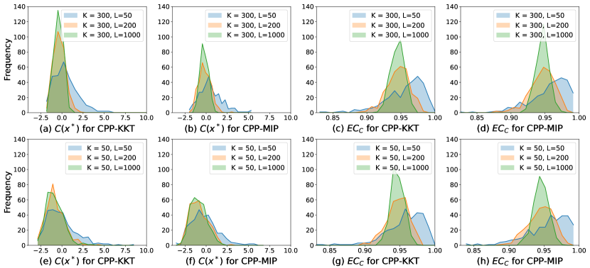
Figure 3: Supplementary Results for the General Nonlinear CCO Problem

Supplementary Results for Feasibility Guarantees. We showcase the effect of the size of the training dataset $K$ and the calibration dataset $L$ on the guarantee in Theorem 3.2 by repeating the second step in the Experimental Procedure from the case study in Section 6. We let $N:=300,V:=1000$. We first fix $K=300$ and vary $L$. We show the empirical distribution of the upper bound $C(x_{2,j}^{*})$ for CPP-KKT in Figure 3(a) and for CPP-MIP in Figure 3(b). We demonstrate the empirical distribution of the empirical coverage $EC_{C,j}$ for CPP-KKT in Figure 3(c) and for CPP-MIP in Figure 3(d). Now, we choose $K=50$ and vary $L$. Similarly, we show the empirical distribution of the upper bound $C(x_{2,j}^{*})$ for CPP-KKT in Figure 3(e) and for CPP-MIP in Figure 3(f). We demonstrate the empirical distribution of the empirical coverage $EC_{C,j}$ for CPP-KKT in Figure 3(g) and for CPP-MIP in Figure 3(h). From the figures, one can infer as expected that the coverage in Theorem 3.2 benefits from a large training and a large calibration size.
Supplementary Results for Average Statistics. We showcase the effect of size of the training dataset $K$ and the calibration dataset $L$ on the computation times by repeating the experimental procedure from the case study in Section 6. We fix $N:=300$ and $V:=1000$ and show in Table LABEL:table:average_statistics the average statistics of the experimental results with $K=50,K=100,K=200,K=300,K=500$ and $L=50,L=200,L=500,L=750,L=1000$.

Table 1: Average Statistics with $N=300$ and $V=1000$ with Varying $K$ and $L$

		$\mathbf{C(x^{*})}$	$\mathbf{J(x^{*})}$	$\mathbf{EC_{0}}$	$\mathbf{EC_{C}}$	Solver Time (s)
K = 50, L = 50	CPP-KKT	0.211	-0.964	0.963	0.961	0.649
	CPP-MIP	0.105	-0.959	0.964	0.959	0.114
K = 50, L = 200	CPP-KKT	-0.49	-0.964	0.963	0.951	0.649
	CPP-MIP	-0.565	-0.959	0.964	0.949	0.114
K = 50, L = 500	CPP-KKT	-0.546	-0.964	0.963	0.95	0.649
	CPP-MIP	-0.62	-0.959	0.964	0.949	0.114
K = 50, L = 750	CPP-KKT	-0.523	-0.964	0.963	0.951	0.649
	CPP-MIP	-0.603	-0.959	0.964	0.95	0.114
K = 50, L = 1000	CPP-KKT	-0.541	-0.964	0.963	0.951	0.649
	CPP-MIP	-0.618	-0.959	0.964	0.95	0.114
K = 100, L = 50	CPP-KKT	0.838	-1.007	0.949	0.96	1.394
	CPP-MIP	0.767	-1.003	0.952	0.962	0.134
K = 100, L = 200	CPP-KKT	0.036	-1.007	0.949	0.949	1.394
	CPP-MIP	0.027	-1.003	0.952	0.951	0.134
K = 100, L = 500	CPP-KKT	-0.009	-1.007	0.949	0.949	1.394
	CPP-MIP	-0.035	-1.003	0.952	0.951	0.134
K = 100, L = 750	CPP-KKT	-0.01	-1.007	0.949	0.95	1.394
	CPP-MIP	-0.025	-1.003	0.952	0.951	0.134
K = 100, L = 1000	CPP-KKT	0.007	-1.007	0.949	0.95	1.394
	CPP-MIP	-0.107	-1.003	0.952	0.949	0.134
K = 200, L = 50	CPP-KKT	0.883	-1.007	0.951	0.963	7.273
	CPP-MIP	0.866	-1.008	0.95	0.962	0.186
K = 200, L = 200	CPP-KKT	0.044	-1.007	0.951	0.95	7.273
	CPP-MIP	0.026	-1.008	0.95	0.949	0.186
K = 200, L = 500	CPP-KKT	-0.062	-1.007	0.951	0.949	7.273
	CPP-MIP	-0.003	-1.008	0.95	0.95	0.186
K = 200, L = 750	CPP-KKT	0.01	-1.007	0.951	0.951	7.273
	CPP-MIP	0.007	-1.008	0.95	0.951	0.186
K = 200, L = 1000	CPP-KKT	-0.043	-1.007	0.951	0.95	7.273
	CPP-MIP	-0.03	-1.008	0.95	0.95	0.186
K = 300, L = 50	CPP-KKT	0.757	-1.008	0.951	0.959	6.476
	CPP-MIP	0.739	-1.009	0.951	0.96	0.225
K = 300, L = 200	CPP-KKT	0.048	-1.008	0.951	0.95	6.476
	CPP-MIP	0.048	-1.009	0.951	0.95	0.225
K = 300, L = 500	CPP-KKT	0.017	-1.008	0.951	0.951	6.476
	CPP-MIP	-0.028	-1.009	0.951	0.95	0.225
K = 300, L = 750	CPP-KKT	-0.023	-1.008	0.951	0.95	6.476
	CPP-MIP	-0.012	-1.009	0.951	0.95	0.225
K = 300, L = 1000	CPP-KKT	-0.046	-1.008	0.951	0.95	6.476
	CPP-MIP	-0.016	-1.009	0.951	0.95	0.225
K = 500, L = 50	CPP-KKT	0.874	-1.012	0.95	0.962	15.093
	CPP-MIP	0.827	-1.01	0.95	0.961	0.326
K = 500, L = 200	CPP-KKT	0.018	-1.012	0.95	0.948	15.093
	CPP-MIP	0.111	-1.01	0.95	0.951	0.326
K = 500, L = 500	CPP-KKT	0.014	-1.012	0.95	0.95	15.093
	CPP-MIP	0.011	-1.01	0.95	0.95	0.326
K = 500, L = 750	CPP-KKT	0.034	-1.012	0.95	0.951	15.093
	CPP-MIP	0.037	-1.01	0.95	0.951	0.326
K = 500, L = 1000	CPP-KKT	0.003	-1.012	0.95	0.95	15.093
	CPP-MIP	-0.004	-1.01	0.95	0.95	0.326

D.2 General Nonlinear CCO Problem: Comparison between CPP, SA, and SAA

Figure 4: Comparison between CPP and SAA

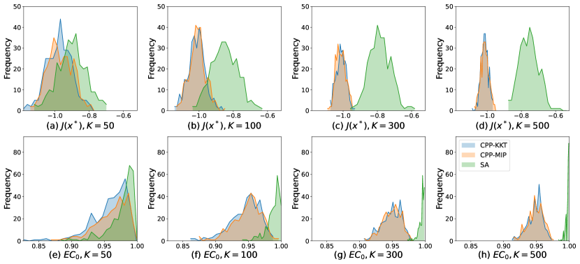
Figure 5: Comparison between CPP and SA

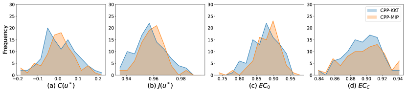
Figure 6: Results for the Optimal Control Problem

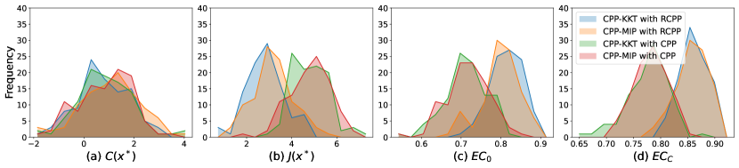
Figure 7: Results for the Portfolio Optimization Problem

We empirically compare our method with the scenario approach (SA) for general nonconvex problems from [23] and the sample average approximation (SAA) approach from [11] on the general nonlinear CCO problem from Section 6. We emphasize that CPP provides marginal probabilistic feasibility guarantees which are different from the feasibility guarantees of SA and SAA making a theoretical comparison difficult. In our comparison, we thus solve the CPP, SA, and SAA problems with the same number of training data $K$. For SA, this may result in conservative solutions.

Recall that in SAA, we approach the CCO problem by enforcing equation (1). In [11], for the approximation in (1), it is shown that for the choice of $\omega<\delta$ a feasibility guarantee can be provided conditioned on the domain of $x$. Under Lipschitz continuity of $f$, this can also be guaranteed by the chance constraint

$$\frac{1}{K}\Sigma_{i=1}^{K}\mathbbm{1}\{f(x,Y^{(i)})+\iota\leq 0\}\geq 1-\omega$$ (26)

for any $\omega<\delta,\iota\in\mathbb{R}>0$ where $\iota$ can be arbitrarily small. As mentioned in Remark (1), CPP shares algorithmic similarities with SAA for the special choice of $\omega=1-\frac{\lceil(K+1)(1-\delta)\rceil}{K}$. To show the similarity, we compare in Figure 4 the results attained by CPP and by SAA (with the choices of $\omega=0.01$ and $\omega=0.03$) for the general nonlinear CCO problem from Section 6 again with $N\coloneqq 300$ and $V\coloneqq 1000$ and for varying $K$. We omit $\iota$ in our comparison, since setting a small $\iota$ will have no practical impact to our experimental results. For a fair comparison, we use the equivalence-preserving MIP encoding introduced in Section 4 for the SAA. In Figure 4, we see that $SAA$ attains similar results to both CPP-KKT and CPP-MIP, especially when $\omega=0.03$, where the selected $\omega$ is closed to $1-\frac{\lceil(K+1)(1-\delta)\rceil}{K}$.

In SA, recall that we require all scenarios $Y^{(i)},\forall i\in\{1,\ldots,K\}$ to satisfy the constraint $f(x,Y^{(i)})\leq 0$ for the decision variable $x$. We compare SA and CPP, again on the general nonlinear CCO problem from Section 6, with varying $K$ in Figure 5 with $N\coloneqq 300$ and $V\coloneqq 1000$. As we expect, we see SA attains more conservative results than CPP, since CPP only requires a portion of the constraints on the scenarios to be satisfied. We remark that a feasibility guarantee exists for SA [23], but we will refrain from comparing to it in this paper since our feasibility guarantees are, as said before, marginal and with respect to $C(x^{*})$.

D.3 Optimal Control Problem: Plots

We show the results for the optimal control case study in Figure 6. The number of timeouts for CPP-KKT and CPP-MIP are $0$ and $16$ respectively. None of the methods have infeasible solution.

D.4 Portfolio Optimization Problem: Plots

To calculate the distribution shift, we use the KL divergence as our choise of f-divergence where $\phi(z)\coloneqq z\log(z)$. We estimate the distribution shift as $\epsilon\coloneqq 0.027$ by computing $D_{\phi}(\tilde{\mathcal{Y}},\mathcal{Y})$ following [63], where a closed-form expression for the KL-divergence is given as

$$D_{\phi}(\mathcal{N}(\mu_{1},\Sigma_{1}),\mathcal{N}(\mu_{2},\Sigma_{2}))=\frac{1}{2}(\text{tr}(\Sigma_{1}^{-1}\Sigma_{2}-I)+(\mu_{1}-\mu_{2})^{T}\Sigma_{1}^{-1}(\mu_{1}-\mu_{2})-\text{logdet}(\Sigma_{2}\Sigma_{1}^{-1})),$$ (27)

where $\mu_{1},\Sigma_{1}$ are the mean and covariance of $\tilde{\mathcal{Y}}$ and $\mu_{2},\Sigma_{2}$ are the mean and convariance of $\mathcal{Y}$. We show the results for the portfolio optimization case study in Figure 7, where we see that our RCPP achieves the expected coverage $EC_{0,j}$ and $EC_{C,j}$, while CPP undercovers and does not account for distribution shift. No timeouts of infeasible solutions are observed for all four methods. The average computation time for CPP-KKT with RCPP, CPP-MIP with RCPP, CPP-KKT with CPP, and CPP-MIP with CPP are 3.05s, 2.28s, 9.26s, 2.54s, respectively.

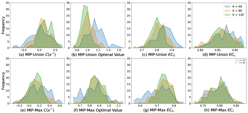
Figure 8: Results for the Case Study for JCCO

D.5 Case Study for JCCO

Problem Statement. In this section, we showcase how to use CPP to solve JCCO problems as explained in Appendix A. We are interested in solving the JCCO problem

$$\min_{x\in\mathbb{R}^{3}} cx$$ (28)

s.t. $$\text{Prob}(Ax-Y\leq\mathbf{0})\geq 1-\delta,$$

$$x\geq\mathbf{0},$$

where $x\in\mathbb{R}^{3}$ is the decision variable, $c=[1,1,1]$, $A=\begin{bmatrix}3&-12&2\\ -10&3&5\\ 5&3&-15\end{bmatrix}$, and $Y$ is a random vector where we fix $Y\sim lst(0,1,10)$ (a Student’s t-distribution) and $\delta:=0.2$. Note that we can use the linear JCCO program in (28) to encode practical problems including the probability set coverage problem [11].
Results. We repeat the experimental procedure from Section 6 with $N\coloneqq 100,V\coloneqq 1000,\text{ and }L\coloneqq 300$ with CPP-MIP using both the union bound (which we refer to as MIP-Union) and the maximum operator (which we refer to as MIP-Max) as introduced in Section D.5. We remark that we do not show the results for CPP-KKT due to the number of timeouts that we observed with the maximum operator encoding while the results for the union bound showed similar results as MIP-Union. We observe no timeout nor infeasible solution with CPP-MIP. We show the empirical distribution of $C(x^{*})$ for MIP-Union in Figure 8(a) and for MIP-Max in Figure 8(e) where both distributions are centered near zero. We highlight that MIP-Union, as expected, is more conservative in terms of the distribution of optimal values, which we show in Figure 8(b), as compared to MIP-Max, shown in Figure 8(f). Since the union bound is more conservative, we see the same trend on their corresponding distributions of $EC_{0}$ and $EC_{c}$ in Figure 8, where MIP-Union attains better coverage results. However, for both distributions, we observe the expected distributions of $EC_{c}$, both of which center above 0.8.

References

- [1] C. Dawson, A. Jasour, A. Hofmann, and B. Williams, “Chance-constrained trajectory optimization for high-dof robots in uncertain environments,” arXiv preprint arXiv:2302.00122, 2023.
- [2] Y. K. Nakka and S.-J. Chung, “Trajectory optimization of chance-constrained nonlinear stochastic systems for motion planning under uncertainty,” IEEE Transactions on Robotics, vol. 39, no. 1, pp. 203–222, 2022.
- [3] L. Blackmore, M. Ono, and B. C. Williams, “Chance-constrained optimal path planning with obstacles,” IEEE Transactions on Robotics, vol. 27, no. 6, pp. 1080–1094, 2011.
- [4] R. N. Sengupta and R. Kumar, “Robust and reliable portfolio optimization formulation of a chance constrained problem,” Foundations of Computing and Decision Sciences, vol. 42, no. 1, pp. 83–117, 2017.
- [5] B. K. Pagnoncelli, S. Ahmed, and A. Shapiro, “Computational study of a chance constrained portfolio selection problem,” Journal of Optimization Theory and Applications, vol. 142, no. 2, pp. 399–416, 2009.
- [6] X. Geng and L. Xie, “Data-driven decision making in power systems with probabilistic guarantees: Theory and applications of chance-constrained optimization,” Annual reviews in control, vol. 47, pp. 341–363, 2019.
- [7] T. Summers, J. Warrington, M. Morari, and J. Lygeros, “Stochastic optimal power flow based on convex approximations of chance constraints,” in 2014 Power Systems Computation Conference. IEEE, 2014, pp. 1–7.
- [8] H. Xu, C. Caramanis, and S. Mannor, “Robust regression and lasso,” Advances in neural information processing systems, vol. 21, 2008.
- [9] S. Pfrommer, T. Gautam, A. Zhou, and S. Sojoudi, “Safe reinforcement learning with chance-constrained model predictive control,” in Learning for Dynamics and Control Conference. PMLR, 2022, pp. 291–303.
- [10] A. Prékopa, Stochastic programming. Springer Science & Business Media, 2013, vol. 324.
- [11] J. Luedtke and S. Ahmed, “A sample approximation approach for optimization with probabilistic constraints,” SIAM Journal on Optimization, vol. 19, no. 2, pp. 674–699, 2008.
- [12] M. C. Campi and S. Garatti, “The exact feasibility of randomized solutions of uncertain convex programs,” SIAM Journal on Optimization, vol. 19, no. 3, pp. 1211–1230, 2008.
- [13] V. Vovk, A. Gammerman, and G. Shafer, Algorithmic learning in a random world. Springer, 2005, vol. 29.
- [14] G. Shafer and V. Vovk, “A tutorial on conformal prediction.” Journal of Machine Learning Research, vol. 9, no. 3, 2008.
- [15] V. Balasubramanian, S.-S. Ho, and V. Vovk, Conformal prediction for reliable machine learning: theory, adaptations and applications. Newnes, 2014.
- [16] A. N. Angelopoulos and S. Bates, “A gentle introduction to conformal prediction and distribution-free uncertainty quantification,” arXiv preprint arXiv:2107.07511, 2021.
- [17] A. Charnes and W. W. Cooper, “Chance-constrained programming,” Management science, vol. 6, no. 1, pp. 73–79, 1959.
- [18] C. Van de Panne and W. Popp, “Minimum-cost cattle feed under probabilistic protein constraints,” Management Science, vol. 9, no. 3, pp. 405–430, 1963.
- [19] S. Kataoka, “A stochastic programming model,” Econometrica: Journal of the Econometric Society, pp. 181–196, 1963.
- [20] A. Prékopa, “Logarithmic concave measures with application to stochastic programming,” Acta Scientiarum Mathematicarum, vol. 32, pp. 301–316, 1971.
- [21] G. C. Calafiore and M. C. Campi, “The scenario approach to robust control design,” IEEE Transactions on automatic control, vol. 51, no. 5, pp. 742–753, 2006.
- [22] M. C. Campi, S. Garatti, and M. Prandini, “The scenario approach for systems and control design,” Annual Reviews in Control, vol. 33, no. 2, pp. 149–157, 2009.
- [23] M. C. Campi, S. Garatti, and F. A. Ramponi, “A general scenario theory for nonconvex optimization and decision making,” IEEE Transactions on Automatic Control, vol. 63, no. 12, pp. 4067–4078, 2018.
- [24] S. Grammatico, X. Zhang, K. Margellos, P. Goulart, and J. Lygeros, “A scenario approach for non-convex control design,” IEEE Transactions on Automatic Control, vol. 61, no. 2, pp. 334–345, 2015.
- [25] G. C. Calafiore, D. Lyons, and L. Fagiano, “On mixed-integer random convex programs,” in 2012 IEEE 51st IEEE Conference on Decision and Control (CDC). IEEE, 2012, pp. 3508–3513.
- [26] M. C. Campi and S. Garatti, “Wait-and-judge scenario optimization,” Mathematical Programming, vol. 167, pp. 155–189, 2018.
- [27] Y. Yang and C. Sutanto, “Chance-constrained optimization for nonconvex programs using scenario-based methods,” ISA transactions, vol. 90, pp. 157–168, 2019.
- [28] J. Luedtke, S. Ahmed, and G. L. Nemhauser, “An integer programming approach for linear programs with probabilistic constraints,” Mathematical programming, vol. 122, no. 2, pp. 247–272, 2010.
- [29] A. Nemirovski and A. Shapiro, “Convex approximations of chance constrained programs,” SIAM Journal on Optimization, vol. 17, no. 4, pp. 969–996, 2007.
- [30] A. Nemirovski, “On safe tractable approximations of chance constraints,” European Journal of Operational Research, vol. 219, no. 3, pp. 707–718, 2012.
- [31] K. Margellos, P. Goulart, and J. Lygeros, “On the road between robust optimization and the scenario approach for chance constrained optimization problems,” IEEE Transactions on Automatic Control, vol. 59, no. 8, pp. 2258–2263, 2014.
- [32] S. Peng, “Chance constrained problem and its applications,” Ph.D. dissertation, Université Paris Saclay (COmUE); Xi’an Jiaotong University, 2019.
- [33] G. C. Calafiore and L. E. Ghaoui, “On distributionally robust chance-constrained linear programs,” Journal of Optimization Theory and Applications, vol. 130, pp. 1–22, 2006.
- [34] E. Delage and Y. Ye, “Distributionally robust optimization under moment uncertainty with application to data-driven problems,” Operations research, vol. 58, no. 3, pp. 595–612, 2010.
- [35] J. Cheng, E. Delage, and A. Lisser, “Distributionally robust stochastic knapsack problem,” SIAM Journal on Optimization, vol. 24, no. 3, pp. 1485–1506, 2014.
- [36] Z. Chen, D. Kuhn, and W. Wiesemann, “Data-driven chance constrained programs over wasserstein balls,” Operations Research, 2022.
- [37] A. R. Hota, A. Cherukuri, and J. Lygeros, “Data-driven chance constrained optimization under wasserstein ambiguity sets,” in 2019 American Control Conference (ACC). IEEE, 2019, pp. 1501–1506.
- [38] R. Ji and M. A. Lejeune, “Data-driven distributionally robust chance-constrained optimization with wasserstein metric,” Journal of Global Optimization, vol. 79, no. 4, pp. 779–811, 2021.
- [39] R. Jiang and Y. Guan, “Data-driven chance constrained stochastic program,” Mathematical Programming, vol. 158, no. 1-2, pp. 291–327, 2016.
- [40] Z. Hu and L. J. Hong, “Kullback-leibler divergence constrained distributionally robust optimization,” Available at Optimization Online, vol. 1, no. 2, p. 9, 2013.
- [41] R. J. Tibshirani, R. Foygel Barber, E. Candes, and A. Ramdas, “Conformal prediction under covariate shift,” Advances in neural information processing systems, vol. 32, 2019.
- [42] A. Lin and S. Bansal, “Verification of neural reachable tubes via scenario optimization and conformal prediction,” arXiv preprint arXiv:2312.08604, 2023.
- [43] R. Koenker and G. Bassett Jr, “Regression quantiles,” Econometrica: journal of the Econometric Society, pp. 33–50, 1978.
- [44] M. Cleaveland, I. Lee, G. J. Pappas, and L. Lindemann, “Conformal prediction regions for time series using linear complementarity programming,” arXiv preprint arXiv:2304.01075, 2023.
- [45] S. P. Boyd and L. Vandenberghe, Convex optimization. Cambridge university press, 2004.
- [46] A. Fischer, “A newton-type method for positive-semidefinite linear complementarity problems,” Journal of Optimization Theory and Applications, vol. 86, pp. 585–608, 1995.
- [47] A. Bemporad and M. Morari, “Control of systems integrating logic, dynamics, and constraints,” Automatica, vol. 35, no. 3, pp. 407–427, 1999.
- [48] T. Achterberg, “Scip: solving constraint integer programs,” Mathematical Programming Computation, vol. 1, pp. 1–41, 2009.
- [49] I. Gibbs and E. Candes, “Adaptive conformal inference under distribution shift,” Advances in Neural Information Processing Systems, vol. 34, pp. 1660–1672, 2021.
- [50] M. Zaffran, O. Féron, Y. Goude, J. Josse, and A. Dieuleveut, “Adaptive conformal predictions for time series,” in International Conference on Machine Learning. PMLR, 2022, pp. 25 834–25 866.
- [51] M. Cauchois, S. Gupta, A. Ali, and J. C. Duchi, “Robust validation: Confident predictions even when distributions shift,” arXiv preprint arXiv:2008.04267, 2020.
- [52] A. Gendler, T.-W. Weng, L. Daniel, and Y. Romano, “Adversarially robust conformal prediction,” in International Conference on Learning Representations, 2021.
- [53] Y. Romano, E. Patterson, and E. Candes, “Conformalized quantile regression,” Advances in neural information processing systems, vol. 32, 2019.
- [54] M. Sesia and E. J. Candès, “A comparison of some conformal quantile regression methods,” Stat, vol. 9, no. 1, p. e261, 2020.
- [55] J. Lei, A. Rinaldo, and L. Wasserman, “A conformal prediction approach to explore functional data,” Annals of Mathematics and Artificial Intelligence, vol. 74, pp. 29–43, 2015.
- [56] L. Guan and R. Tibshirani, “Prediction and outlier detection in classification problems,” Journal of the Royal Statistical Society Series B: Statistical Methodology, vol. 84, no. 2, pp. 524–546, 2022.
- [57] W. Xie, S. Ahmed, and R. Jiang, “Optimized bonferroni approximations of distributionally robust joint chance constraints,” Mathematical Programming, vol. 191, no. 1, pp. 79–112, 2022.
- [58] L. Lindemann, M. Cleaveland, G. Shim, and G. J. Pappas, “Safe planning in dynamic environments using conformal prediction,” IEEE Robotics and Automation Letters, 2023.
- [59] V. Raman, A. Donzé, M. Maasoumy, R. M. Murray, A. Sangiovanni-Vincentelli, and S. A. Seshia, “Model predictive control with signal temporal logic specifications,” in 53rd IEEE Conference on Decision and Control. IEEE, 2014, pp. 81–87.
- [60] A. K. Kuchibhotla, “Exchangeability, conformal prediction, and rank tests,” arXiv preprint arXiv:2005.06095, 2020.
- [61] R. Koenker, Quantile regression. Cambridge university press, 2005, vol. 38.
- [62] Y. Zhao, B. Hoxha, G. Fainekos, J. V. Deshmukh, and L. Lindemann, “Robust conformal prediction for stl runtime verification under distribution shift,” arXiv preprint arXiv:2311.09482, 2023.
- [63] L. Devroye, A. Mehrabian, and T. Reddad, “The total variation distance between high-dimensional gaussians with the same mean,” arXiv preprint arXiv:1810.08693, 2018.