Abstract.

There are several ways to establish the asymptotic normality of $L$-statistics, depending upon the selection of the weights generating function and the cumulative distribution function of the underlying model. Here, in this paper it is shown that the two of the asymptotic approaches are equivalent/equal for a particular choice of the weights generating function.

Keywords. Asymptotic normality; Equivalency; $L$-statistics; Robustness; Trimmed moments.

1 Introduction

For a positive integer $n$, let $X_{1},\ldots,X_{n}$ be an iid sample from an unknown true underlying cumulative distribution function $F$ with the parameter vector $\bm{\theta}=(\theta_{1},\cdots,\theta_{k})$. The motivation of most of the statistical inference is to estimate the parameter vector $\bm{\theta}$ from the available sample dataset. The corresponding order statistic of the sample is denoted by $X_{1:n},\ldots,X_{n:n}$. In order to estimate the parameter vector $\bm{\theta}$, the statistics we are interested here is a linear combination of the order values, so the name $L$-statistics, in the form

$$\widehat{\mu}_{j} :=\dfrac{1}{n}\sum_{i=1}^{n}J_{j}\left(\dfrac{i}{n+1}\right)h_{j}(X_{i:n}),\quad 1\leq j\leq k,$$ (1)

where $J_{j}:[0,1]\to\mathbb{R}_{\geq 0}$ represents a weights-generating. Both $J_{j}$ and $h_{j}$ are specially chosen functions, (see, e.g., Poudyal, 2021, Poudyal and Brazauskas, 2022) and are known that are specified by the statistician.

The corresponding population qualities are then given by

$$\mu_{j} \equiv\mu_{j}\left(\bm{\theta}\right)\equiv\mu_{j}\left(\theta_{1},\ldots,\theta_{k}\right)=\int_{0}^{1}{J_{j}(u)H_{j}(u)\,du,\quad 1\leq{j}\leq{k}},\mbox{ where }H_{j}:=h_{j}\circ F^{-1}.$$ (2)

Like classical method of moments, $L$-estimators are found by matching sample $L$-moments, Eq. (1), with population $L$-moments, Eq. (2), for $j=1,\ldots,k$, and then solving the system of equations with respect to $\theta_{1},\ldots,\theta_{k}$. The obtained solutions, which we denote by $\widehat{\theta}_{j}=\tau_{j}(\widehat{\mu}_{1},\ldots,\widehat{\mu}_{k})$, $1\leq j\leq k$, are, by definition, the $L$-estimators of $\theta_{1},\ldots,\theta_{k}$. Note that the functions $\tau_{j}$ are such that $\theta_{j}=\tau_{j}(\mu_{1}(\bm{\theta}),\ldots,\mu_{k}(\bm{\theta})).$

Further, define

$$\alpha_{j}(u) =\frac{1}{1-u}\int_{u}^{1}g_{j}(v)(1-v)\,dv,\quad\mbox{where}\quad g_{j}(v):=J_{j}(v)H_{j}^{\prime}(v),\quad 1\leq{j}\leq{k}.$$ (3)

Consider

$$\widehat{\bm{\mu}}:=\left(\widehat{\mu}_{1},\widehat{\mu}_{1},\ldots,\widehat{\mu}_{k}\right)\quad\mbox{and}\quad\bm{\mu}:=\left(\mu_{1},\mu_{2},\ldots,\mu_{k}\right).$$

Ideally, we expect that the statistics vector $\widehat{\bm{\mu}}$ converges in distribution to the population vector $\bm{\mu}$. As mentioned by Serfling (1980, §8.2 and references therein), there are several approaches of establishing asymptotic normality of $\widehat{\bm{\mu}}$ depending upon the various scenarios of the weights generating function $J$ and the underlying cdf $F$. This paper focuses only on a specific weights generating function $J$.

In particular, Chernoff et al. (1967, Remark 9) established that the $k$-variate vector $\sqrt{n}(\widehat{\bm{\mu}}-\bm{\mu})$, converges in distribution to the $k$-variate normal random vector with mean $\mathbf{0}$ and the variance-covariance matrix $\mathbf{\Sigma}:=\left[\sigma_{ij}^{2}\right]_{i,j=1}^{k}$ with the entries

$$\sigma_{ij}^{2} =\int_{0}^{1}{\alpha_{i}(u)\alpha_{j}(u)\,du}$$ (4)

$$=\int_{0}^{1}{\left(\frac{1}{1-u}\right)^{2}\left[\int_{u}^{1}{g_{i}(v)(1-v)}\,dv\int_{u}^{1}{g_{j}(w)(1-w)}\,dw\right]du}$$ (5)

$$=\int_{0}^{1}\int_{0}^{1}g_{i}(v)g_{j}(w)K(v,w)\,dv\,dw,$$ (6)

where the function $K(v,w)$ is defined as

$$K(v,w) :=K(w,v)=v\wedge w-vw=\min\{v,w\}-vw,\quad\mbox{for}\quad 0\leq v\leq w\leq 1.$$ (7)

For given $0\leq a_{j}<1-b_{j}\leq 1$, and with the specific weights-generating function

$$J_{j}(s) =\left\{\begin{array}[]{ll}(1-a_{j}-b_{j})^{-1},&a_{j}<s<1-b_{j};\\ 0,&\text{otherwise},\\ \end{array}\right.\quad 1\leq j\leq k,$$ (10)

the sample $L$-moments, Eq. (1), and the population $L$-moments, Eq. (2) are simply the sample and population trimmed moments, respectively. For these specific weights-generating functions, Brazauskas et al. (2007, 2009) independently established an equivalent simplified expression for $\sigma_{ij}^{2}$, which can be written as

$$\sigma_{ij}^{2} =\Gamma\int_{a_{i}}^{1-b_{i}}\int_{a_{j}}^{1-b_{j}}{K(v,w)}\ dh_{j}(F^{-1}(v))\ dh_{i}(F^{-1}(w)),\quad\Gamma:=\prod_{r=i,j}\left(1-a_{r}-b_{r}\right)^{-1}.$$ (11)

The motivation of this paper is to show the equivalency of the Eqs. (4), (5), (6), and (11).

2 Preliminaries

In order to establish the equivalency of the different approaches mentioned in Section 1, we summarize essential measure theoretic preliminaries in this section.

Let $E\subseteq\mathbb{R}^{2}$ and $f:E\to\mathbb{R}$ are Lebesgue measurable set and function, respectively. Then, following Folland (1999, p. 65), we define

$$\mbox{For a fixed $x$, {\bf$x$-section}}: \quad E_{x}:=\left\{y\in\mathbb{R}:(x,y)\in E\right\}\quad\mbox{and}\quad f_{x}(y):=f(x,y),$$ (12)

$$\mbox{For a fixed $y$, {\bf$y$-section}}: \quad E_{y}:=\left\{x\in\mathbb{R}:(x,y)\in E\right\}\quad\mbox{and}\quad f_{y}(x):=f(x,y).$$ (13)

It is well known that, Fubini’s Theorem provides a crucial link between multiple integrals and iterated integrals, assuming the function involved is integrable. Essentially, it enables evaluation of double integrals by swapping the order of integration (and, by extension, multiple integrals) as iterated one dimensional integrals. Here, we state the Fubini’s Theorem without introducing the concept of product measure.

Theorem 1 (Fubini’s Theorem - Folland (1999), p. 67).

Let $E:=[a,b]\times[c,d]\subseteq\mathbb{R}^{2}$, s.t. $a<b$ and $c<d$, is a rectangular region. Consider a function

$$f:E\to\mathbb{R}\quad\mbox{s.t.}\quad\int_{E}\left|f(x,y)\right|\,dy\,dx<\infty,$$

then the Fubini’s Theorem states that

$$\int_{a}^{b}\int_{c}^{d}f(x,y)\,dy\,dx =\int_{E_{x}}\left(\int_{E_{y}}f(x,y)\,dy\right)\,dx=\int_{E_{y}}\left(\int_{E_{x}}f(x,y)\,dx\right)\,dy,$$ (14)

$$\mbox{i.e.,}\quad\int_{E}f(x,y)\,dy\,dx =\int_{E_{x}}\left(\int_{E_{y}}f_{x}(y)\,dy\right)\,dx=\int_{E_{y}}\left(\int_{E_{x}}f_{y}(x)\,dx\right)\,dy.$$ (15)

An immediate application of the Fubini’s Theorem is the following corollary.

Corollary 1.

Let $g_{1}:\mathbb{R}\to\mathbb{R}$ and $g_{2}:\mathbb{R}\to\mathbb{R}$ are two integrable functions in the finite interval $[a,b]$ with $a<b$ such that

$$\int_{E}\left|g_{1}(x)g_{2}(y)\right|\,dy\,dx<\infty,$$

where $E=[a,b]\times[a,b]$. Then it follows that

$$\left(\int_{a}^{b}g_{1}(x)\,dx\right)\left(\int_{a}^{b}g_{2}(y)\,dy\right) =\int_{E}g_{1}(x)g_{2}(y)\,dy\,dx=\int_{a}^{b}\int_{a}^{b}g_{1}(x)g_{2}(y)\,dy\,dx.$$ (16)

In particular if $g_{1}\equiv g_{2}=g$, then Eq. (16) takes the form

$$\left(\int_{a}^{b}g(x)\,dx\right)^{2} =\left(\int_{a}^{b}g(x)\,dx\right)\left(\int_{a}^{b}g(y)\,dy\right)=\int_{a}^{b}\int_{a}^{b}g(x)g(y)\,dy\,dx.$$ (17)

3 Main Results

Here, we establish the equivalency of the two asymptotic approaches for the weights-generating function given by Eq. (10). That is, we establish the equivalency of the Eqs. (4), (5), (6), and (11).

Eq. (5) follows obviously from (4).

Eq. (5) $\implies$ Eq. (6): From Corollary 1, we have

$$\alpha_{i}(u)\alpha_{j}(u) =\left(\frac{1}{1-u}\right)^{2}\left[\int_{u}^{1}{g_{i}(v)(1-v)}\,dv\int_{u}^{1}{g_{j}(w)(1-w)}\,dw\right]$$ (18)

$$=\left(\frac{1}{1-u}\right)^{2}\int_{u}^{1}\int_{u}^{1}g_{i}(v)g_{j}(w)(1-v)(1-w)\,dv\,dw.$$ (19)

Then from Eq. (5), it follows that

$$\sigma_{ij}^{2} =\int_{0}^{1}\left(\frac{1}{1-u}\right)^{2}\left[\int_{u}^{1}\int_{u}^{1}g_{i}(v)(1-v)g_{j}(w)(1-w)\,dv\,dw\right]\,du$$

$$=\int_{\Omega}g_{i}(v)g_{j}(w)\left(\frac{1}{1-u}\right)^{2}(1-v)(1-w)\,dv\,dw\,du,$$ (20)

where the domain of integration, $\Omega\subset[0,1]^{3}$, in Eq. (20), is defined as

$$\Omega :=\left\{0\leq u\leq 1,\ u\leq v\leq 1,\ u\leq w\leq 1\right\}$$

$$=\left\{0\leq x\leq v\wedge w,\ 0\leq v\leq 1,\ 0\leq w\leq 1,\right\}\subseteq\mathbb{R}^{3}.$$ (21)

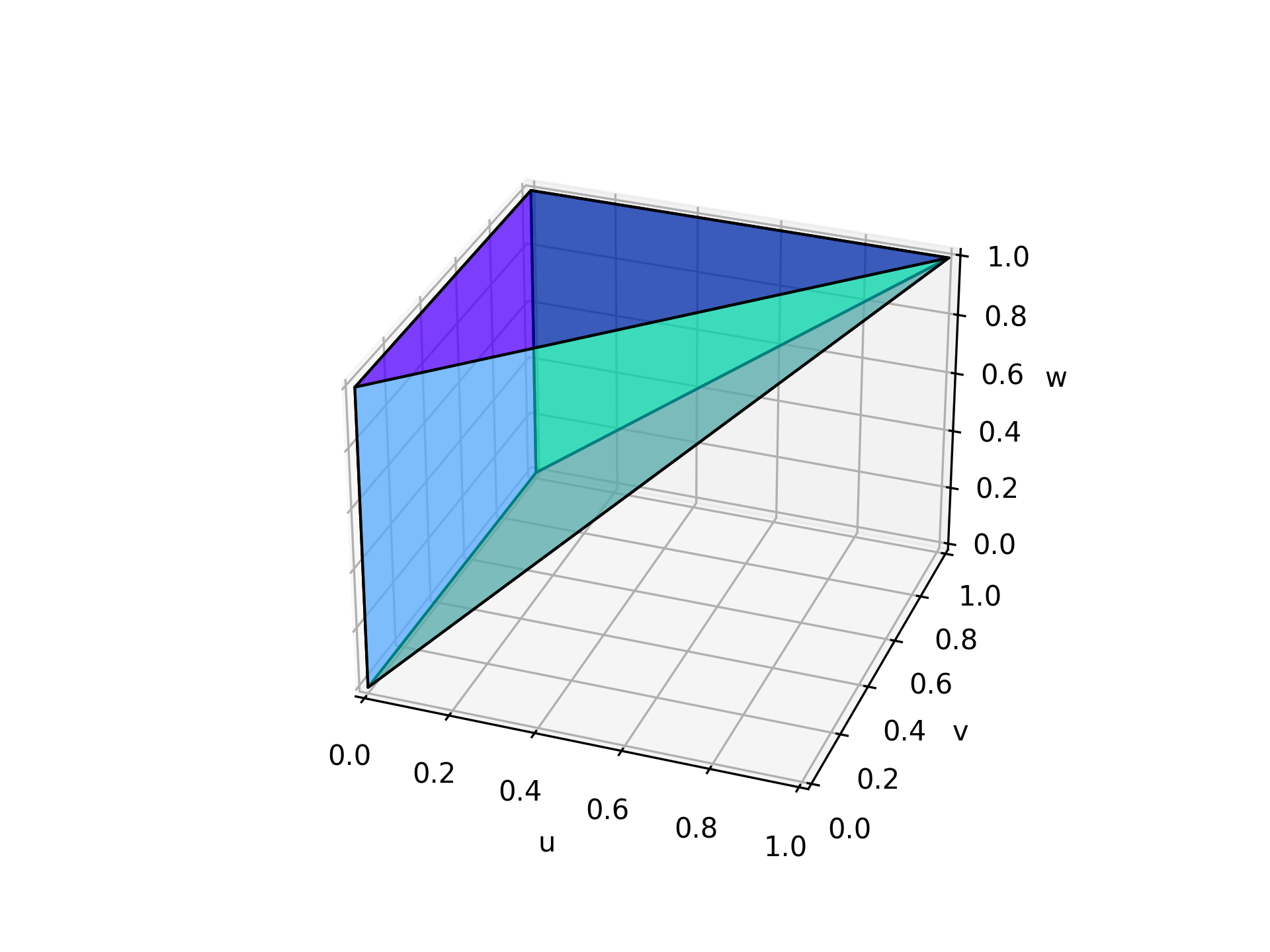
Figure 1: Visualization of the set $\Omega$.

It is clear that $\Omega$ – a rectangular pyramid as shown in Figure 1, is a measurable subset of the unit cube $[0,1]^{3}$. That is, the Lebesgue measure of $\Omega$ is simply the volume of $\Omega$ which is 1/3. Also, note that $\Omega_{u}=v\wedge w$, $\Omega_{v}=[0,1]$, and $\Omega_{w}=[0,1]$. Since $\Omega$ is measurable and assuming the functions involved in Eq. (20) satisfy the conditions for Fubini’s Theorem, then the order of integration in Eq. (20) can be changed. That is,

$$\sigma_{ij}^{2} =\int_{\Omega}g_{i}(v)g_{j}(w)\left(\frac{1}{1-u}\right)^{2}(1-v)(1-w)\,dv\,dw\,du$$

$$=\int_{\Omega_{u}}\int_{\Omega_{w}}\int_{\Omega_{v}}g_{i}(v)g_{j}(w)\left(\frac{1}{1-u}\right)^{2}(1-v)(1-w)\,dv\,dw\,du$$

$$=\int_{\Omega_{w}}\int_{\Omega_{v}}\int_{\Omega_{u}}g_{i}(v)g_{j}(w)\left(\frac{1}{1-u}\right)^{2}(1-v)(1-w)\,du\,dv\,dw$$

$$=\int_{\Omega_{w}}\int_{\Omega_{v}}g_{i}(v)g_{j}(w)\left(\int_{\Omega_{u}}\left(\frac{1}{1-u}\right)^{2}\,du\right)(1-v)(1-w)\,dv\,dw$$

$$=\int_{\Omega_{w}}\int_{\Omega_{v}}g_{i}(v)g_{j}(w)\left.\left(\frac{1}{1-u}\right)\right|_{u=0}^{u=v\wedge w}(1-v)(1-w)\,dv\,dw$$

$$=\int_{\Omega_{w}}\int_{\Omega_{v}}g_{i}(v)g_{j}(w)\left(\frac{1}{1-v\wedge w}-1\right)(1-v)(1-w)\,dv\,dw.$$ (22)

As observed in Eq. (22), in order to establish Eq. (5) $\implies$ Eq. (6), it simply remains to show that

$$K(v,w) =v\wedge w-vw=\left(\frac{1}{1-v\wedge w}-1\right)(1-v)(1-w).$$ (23)

To establish this equality, we investigate in two scenarios.

• If $v\leq w$, then $v\wedge w=v$ and we get

  $$\left(\frac{1}{1-v\wedge w}-1\right)(1-v)(1-w)=\left(\frac{1}{1-v}-1\right)(1-v)(1-w)=v-vw=K(v,w).$$

• If $v>w$, then $v\wedge w=v$ and it follows that

  $$\left(\frac{1}{1-v\wedge w}-1\right)(1-v)(1-w)=\left(\frac{1}{1-w}-1\right)(1-v)(1-w)=w-vw=K(v,w).$$

Therefore, Eq. (22) takes the form

$$\sigma_{ij}^{2} =\int_{\Omega_{w}}\int_{\Omega_{v}}g_{i}(v)g_{j}(w)\left(\frac{1}{1-v\wedge w}-1\right)(1-v)(1-w)\,dv\,dw$$

$$=\int_{\Omega_{w}}\int_{\Omega_{v}}g_{i}(v)g_{j}(w)K(v,w)\,dv\,dw$$

$$=\int_{0}^{1}\int_{0}^{1}g_{i}(v)g_{j}(w)K(v,w)\,dv\,dw,$$ (24)

which is Eq. (6) as desired.

Eq. (6) $\implies$ Eq. (11): As observed in Eq. (2), first, we note that

$$H_{j}(u) =h_{j}(F^{-1}(u))\quad\implies\quad H_{j}^{\prime}(u)du=dh_{j}(F^{-1}(u)).$$ (25)

Now, for the special weight function given by Eq. (10), then Eq. (6) coverts to

$$\sigma_{ij}^{2} =\int_{0}^{1}\int_{0}^{1}g_{i}(v)g_{j}(w)K(v,w)\,dv\,dw$$ (26)

$$=\int_{0}^{1}\int_{0}^{1}J_{j}(v)J_{i}(w)K(v,w)\,dh_{j}(F^{-1}(v))\,dh_{i}(F^{-1}(w))$$

$$=\Gamma\int_{a_{i}}^{1-b_{i}}\int_{a_{j}}^{1-b_{j}}K(v,w)\,dh_{j}(F^{-1}(v))\,dh_{i}(F^{-1}(w))$$

$$=\Gamma\int_{a_{i}}^{1-b_{i}}\int_{a_{j}}^{1-b_{j}}\left[\text{min}\>\{v,w\}-vw\right]dh_{j}(F^{-1}(v))\,dh_{i}(F^{-1}(w))$$

$$=\Gamma\int_{a_{i}}^{1-b_{i}}\int_{a_{j}}^{1-b_{j}}\left[v\wedge w-vw\right]dh_{j}(F^{-1}(v))\,dh_{i}(F^{-1}(w)),$$ (27)

which is exactly Eq. (11).

References

• Brazauskas etΒ al. (2007) Brazauskas, V., Jones, B.L., and Zitikis, R. (2007). Robustification and performance evaluation of empirical risk measures and other vector-valued estimators. METRON–International Journal of Statistics, 65(2), 175–199.
• Brazauskas etΒ al. (2009) Brazauskas, V., Jones, B.L., and Zitikis, R. (2009). Robust fitting of claim severity distributions and the method of trimmed moments. Journal of Statistical Planning and Inference, 139(6), 2028–2043.
• Chernoff etΒ al. (1967) Chernoff, H., Gastwirth, J.L., and Johns, Jr., M.V. (1967). Asymptotic distribution of linear combinations of functions of order statistics with applications to estimation. Annals of Mathematical Statistics, 38(1), 52–72.
• Folland (1999) Folland, G.B. (1999). Real Analysis: Modern Techniques and Their Applications. Second edition. John Wiley & Sons, New York.
• Poudyal (2021) Poudyal, C. (2021). Robust estimation of loss models for lognormal insurance payment severity data. ASTIN Bulletin. The Journal of the International Actuarial Association, 51(2), 475–507.
• Poudyal and Brazauskas (2022) Poudyal, C. and Brazauskas, V. (2022). Robust estimation of loss models for truncated and censored severity data. Variance – The scientific journal of the Casualty Actuarial Society, 15(2), 1–20.
• Serfling (1980) Serfling, R.J. (1980). Approximation Theorems of Mathematical Statistics. John Wiley & Sons, New York.