Replicability is Asymptotically Free in Multi-armed Bandits

Abstract

This work is motivated by the growing demand for reproducible machine learning. We study the stochastic multi-armed bandit problem. In particular, we consider a replicable algorithm that ensures, with high probability, that the algorithm’s sequence of actions is not affected by the randomness inherent in the dataset. We observe that existing algorithms require $O(1/\rho^{2})$ times more regret than nonreplicable algorithms, where $\rho$ is the level of nonreplication. However, we demonstrate that this additional cost is unnecessary when the time horizon $T$ is sufficiently large for a given $\rho$, provided that the magnitude of the confidence bounds is chosen carefully. We introduce an explore-then-commit algorithm that draws arms uniformly before committing to a single arm. Additionally, we examine a successive elimination algorithm that eliminates suboptimal arms at the end of each phase. To ensure the replicability of these algorithms, we incorporate randomness into their decision-making processes. We extend the use of successive elimination to the linear bandit problem as well. For the analysis of these algorithms, we propose a principled approach to limiting the probability of nonreplication. This approach elucidates the steps that existing research has implicitly followed. Furthermore, we derive the first lower bound for the two-armed replicable bandit problem, which implies the optimality of the proposed algorithms up to a $\log\log T$ factor for the two-armed case.

1 Introduction

The multi-armed bandit (MAB) problem is one of the most well-known instances of sequential decision-making problems in uncertain environments, which can model various real-world scenarios. The problem involves conceptual entities called arms, of which there are a total of $K$. At each round $t=1,2,\dots$, the forecaster selects one of the $K$ arms and receives a corresponding reward. The forecaster’s objective is to maximize the cumulative reward over these rounds. Maximizing this cumulative reward is equivalent to minimizing regret, the difference between the forecaster’s cumulative reward and the reward of the best arm. The initial investigation of this problem took place within the field of statistics (Thompson, 1933; Robbins, 1952). In the past two decades, the machine learning community has conducted extensive research in this area, driven by numerous applications, including website optimization, A/B testing, and the formulation of meta-algorithms for algorithmic procedures (Auer et al., 2002; Li et al., 2010; Komiyama et al., 2015; Li et al., 2017).

Several algorithms have proven to be effective. Notably, the upper confidence bound (UCB, Lai and Robbins, 1985; Auer et al., 2002) and Thompson sampling (TS, Thompson, 1933) are widely recognized. Research has shown that these algorithms are asymptotically optimal (Cappé et al., 2013; Agrawal and Goyal, 2012; Kaufmann et al., 2012) in terms of regret, which means that these efficient algorithms exploit accumulated reward information to the fullest extent possible.

1.1 Replicability

One possible drawback of such efficiency is the algorithm’s stability when dealing with small changes in the dataset, which can make replicating results challenging. To illustrate this, consider the following example:

Example 1.1.

(Crowdsourcing (Abraham et al., 2013; Tran-Thanh et al., 2014)) Imagine a company conducting a crowd-based A/B testing with $K$ items. In this scenario, each round $t$ corresponds to a worker visiting their website, and each reward represents the feedback provided by the worker, such as a five-star rating. The key statistic of interest here is the mean score given by the workers. By using UCB or TS to allocate an item to each user, the system can quickly eliminate unpopular items from the candidate set. Although the company aims to publish the results, it is reluctant to disclose all the specific details of the setup. Therefore, it provides the experimental protocol along with summary statistics.

In Example 1.1, the original dataset is not disclosed, making it impossible for an external institution to perfectly replicate the experiment. To address this lack of guarantee due to the vague dataset specification, we focus on the algorithm’s stability. Broadly speaking, a stable algorithm is robust against minor changes in the dataset. Notable categories of stability encompass differential privacy (Dwork et al., 2014), worst-case and average sensitivity (Varma and Yoshida, 2021), and pseudo-determinicity (Gat and Goldwasser, 2011). Among these notions of stability, we consider the replicability (Impagliazzo et al., 2022) in this work. In simple terms, a replicable algorithm exhibits almost identical behavior on two datasets sharing the same data-generating process. This concept aligns well with Example 1.1, where the data-generating process is clearly defined as a material method, whereas the dataset itself remains undisclosed.

Another advantage of promoting replicability in the context of sequential learning is its relation to statistical testing. It is well-known that the standard frequentist confidence interval no longer holds for the results of the multi-armed bandit problem because such an adaptive algorithm violates the assumption of statistical testing that the number of samples is fixed. In general, mean statistics derived from the multi-armed bandit algorithm are downward biased (Xu et al., 2013; Shin et al., 2019), and this bias persists even for a large sample scheme (Lai and Wei, 1982), rendering the use of standard confidence intervals ineffective even for asymptotics (Deshpande et al., 2018). Replicability is one of the best methods to address such bias because it forces the algorithm to exhibit identical behavior in multiple runs with different datasets sharing a common underlying data-generating process.

Table 1: Comparison of regret bounds in the $K$-armed and linear bandit problems. Means $\{\mu_{i}\}_{i\in[K]}$ are sorted in descending order, $\Delta_{i}=\mu_{1}-\mu_{i}$ is the suboptimality gap of the arm $i$, and $\Delta=\Delta_{2}$. The RSE algorithm is referenced multiple times, which implies that it has the smallest regret among the bounds. The lower bound is derived for the case with two arms. Here, $\tilde{O}$ omits a polylog factor in $d,K,T$.

Problem	Esfandiari et al. (2023a)	This work
$K$-armed	$O\left(\sum_{i=2}^{K}\frac{1}{\Delta_{i}}\frac{K^{2}\log T}{\rho^{2}}\right)$	$O\left(\sum_{i=2}^{K}\frac{\Delta_{i}}{\Delta^{2}}\left(\log T+\frac{\log(K(\log T)/\rho)}{\rho^{2}}\right)\right)$         (REC (Theorem 3) and RSE (Theorem 4)) $O\left(\sum_{i=2}^{K}\frac{1}{\Delta_{i}}\left(\log T+\frac{K^{2}\log(K(\log T)/\rho)}{\rho^{2}}\right)\right)$         (RSE, Theorem 4) $O\left(\sqrt{KT\left(\log T+\frac{K^{2}\log(K(\log T)/\rho)}{\rho^{2}}\right)}\right)$         (RSE, Theorem 4) $\Omega\left(\left(\frac{1}{\Delta}\right)\max\left(\log T,\frac{1}{\rho^{2}\log((\rho\Delta)^{-1})}\right)\right)$         (Lower bound, Theorem 5)
Linear	$\tilde{O}\left(\frac{K^{2}\sqrt{dT}}{\rho^{2}}\right)$	$O\left(\frac{d}{\Delta^{2}}\left(\log T+\frac{\log(K(\log T)/\rho)}{\rho^{2}}\right)\right)$ (RLSE, Theorem 8) $\tilde{O}\left(\frac{dK}{\rho}\sqrt{T}\right)$ (RLSE, Theorem 8)

1.2 Our Contributions

The concept of replicability in learning was formalized by Impagliazzo et al. (2022). As far as we know, Esfandiari et al. (2023a) is the sole work that provides algorithms studying replicability for the multi-armed bandit problem. The regret of the algorithms therein is

$$O\left(\sum_{i=2}^{K}\frac{1}{\Delta_{i}}\frac{K^{2}\log T}{\rho^{2}}\right),$$ (1)

which is $K^{2}/\rho^{2}$ times larger than that of nonreplicable algorithms, such as UCB and TS. Here, $K$ is the number of arms, $T$ is the number of rounds, $\Delta_{i}$ is the suboptimality gap for arm $i$, and $\rho$ is the probability of nonreplication. Although the additional factor might appear necessary for the cost of replicability, it is somewhat disappointing to pay such a cost for replication. Upon closer examination of the problem, we discovered that the cost for the replicability can be decoupled from the original regret. Namely, we obtain regret of

$$O\Biggl{(}\underbrace{\sum_{i=2}^{K}\frac{1}{\Delta_{i}}\log T}_{\text{Regret for nonreplicable bandits}}+\ \ \ \underbrace{\sum_{i=2}^{K}\frac{1}{\Delta_{i}}\frac{K^{2}\log(K(\log T)/\rho)}{\rho^{2}}}_{\text{Regret for replicability}}\ \Biggr{)}.$$ (2)

This equation 2 is encouraging in the following sense. When we fix $K,\rho$ and consider sufficiently large $T$, then the $O(\log T)$ first term dominates the $O(\log\log T)$ second term. If we ignore the second term, we obtain a regret of $O(\sum_{i=2}^{K}\frac{\log T}{\Delta_{i}})$, which matches the optimal rate of regret in stochastic bandits. Although equation 2 may not always be the prevailing bound, it is substantially more effective than the existing bound in equation 1. This improvement is attributed to how the factors $\log T$ and $K^{2}/\rho^{2}$ are decomposed. To elaborate further, the algorithmic contributions of this work are outlined as follows.

• After the problem setup (Section 2), we introduce a principled framework for bounding nonreplication probability, which is often used implicitly in the literature (Section 3). The framework is quite general and can be extended into a more general class of sequential learning problems, such as episodic reinforcement learning.

• We then introduce the Replicable Explore-then-Commit (REC) algorithm (Section 4), which has a regret bound of

  $$O\left(\sum_{i=2}^{K}\frac{\Delta_{i}}{\Delta^{2}}\log T+\sum_{i=2}^{K}\frac{\Delta_{i}}{\Delta^{2}}\frac{\log(K(\log T)/\rho)}{\rho^{2}}\right).$$ (3)

  The advantage of  equation 3 is that both terms are $\tilde{O}(K)$, which is better than equation 2 when the suboptimality gaps for each arm are within a constant factor.

• However, depending on the suboptimality gaps,  equation 3 can be arbitrarily worse compared with existing bound of  equation 1. To deal with this issue, we introduce the Replicable Successive Elimination (RSE) algorithm (Section 5) regret bound is the minimum of equation 2 and equation 3. Furthermore, based on these bounds, we derive a distribution-independent regret bound for the replicable $K$-armed bandit problem.

• We derive the first lower bound for the replicable $K$-armed bandits (Section 6) that implies the optimality of equation 2 for $K=2$ up to a logarithmic factor of $K,\rho,\Delta$, and $\log T$.

• We further consider the linear bandit problem (Section 7), in which each of the $K$ arms is associated with $d<K$ features. We show that a rather straightforward modification of RSE yields an algorithm with a regret bound of $O(d)$, independent of $K$.

The performance of REC and RSE are supported by simulations (Section 8). A comparison of existing algorithms and our algorithms is summarized in Table 1.

2 Problem Setup

We consider the finite-armed stochastic bandit problem with $T$ rounds. At each round $t$, the forecaster who adopts an algorithm selects one of the arms $I_{t}\in[K]:=\{1,2,3,\dots,K\}$ and receives the corresponding reward $r_{t}$. Each arm $i\in[K]$ has an (unknown) mean parameter $\mu_{i}\in\mathbb{R}$. Here, $\mu_{i}\in[a,b]$ for some $a,b\in\mathbb{R}$ and let $S=b-a$. We assume $S$ to be a constant. The reward at round $t$ is $r_{t}=\mu_{I_{t}}+\eta_{t},$ where $\eta_{t}$ is a $\sigma$-subgaussian random variable that is independently drawn at each round. The subgaussian assumption is quite general that is not limited to Gaussian random variables. Any bounded random variable is subgaussian, and thus, it is capable of representing binary events (Yes or No) and ordered choice (e.g., 5-star rating). For subgaussian random variables, the following inequality holds.

Lemma 1 (Concentration inequality).

Let $X_{1},X_{2},\ldots,X_{N}$ be $N$ independent (zero-mean) $\sigma$-subgaussian random variables, and $\hat{\mu}_{N}=(1/N)\sum_{i}X_{i}$ be the empirical mean. Then, for any ${\epsilon}>0$ we have

$$\mathbb{P}\left[|\hat{\mu}_{N}|\geq{\epsilon}\right]\leq 2\exp\left(\frac{-{\epsilon}^{2}N}{2\sigma^{2}}\right).$$ (4)

For ease of discussion, we assume the mean reward of each arm is distinct. In this case, we can assume $\mu_{1}>\mu_{2}>\dots>\mu_{K}$ without loss of generality. Of course, an algorithm cannot exploit this ordering. A quantity called regret is defined as follows:

$$\mathrm{Regret}(T):=\sum_{t\in[T]}(\mu_{1}-\mu_{I_{t}})=\sum_{i\in[K]}\Delta_{i}N_{i}(T),$$

where $\Delta_{i}=\mu_{1}-\mu_{i}$ and $N_{i}(T)$ is the number of draws on arm $i$ during the $T$ rounds. We also denote $\Delta=\min_{i\geq 2}\Delta_{i}=\Delta_{2}$. The performance of an algorithm is measured by the expected regret, where the expectation is taken over (hypothetical) multiple runs. Before discussing the replicability, we formalize the notion of dataset in a sequential learning problem because the reward $r_{t}$ in the aforementioned procedure is drawn adaptively upon the choice of the arm $I_{t}$. The fact that each noise term $\eta_{t}$ is drawn independently enables us to reformulate the problem as follows:

Definition 2.1.

(Dataset) The process of the multi-armed bandit problem is equivalent to the following: First, draw a matrix $(r_{i,n})_{i\in[K],n\in[T]}$, where $r_{i,n}=\mu_{i}+\eta_{i,n}$ and $\eta_{i,n}$ are an independent $\sigma$ subgaussian random variable. Second, run a multi-armed bandit problem. Here, $r_{t}$ is the $(I_{t},N_{I_{t}}(t))$-entry of the matrix. We call this matrix a dataset and denote it as $\mathcal{D}$. We call $(\mu_{i})_{i\in[K]}$ a data-generating process or a model.

Following Esfandiari et al. (2023a), we consider the class of replicable algorithms that, with high probability, gives exactly the same sequence of selected arms for two independent runs.

Definition 2.2.

($\rho$-replicability, Impagliazzo et al. 2022; Esfandiari et al. 2023a) For $\rho\in[0,1]$, an algorithm is $\rho$-replicable if,

$$\mathbb{P}_{U,\mathcal{D}^{(1)},\mathcal{D}^{(2)}}\left[(I^{(1)}_{1},I^{(1)}_{2},\dots,I^{(1)}_{T})=(I^{(2)}_{1},I^{(2)}_{2},\dots,I^{(2)}_{T})\right]\geq 1-\rho,$$ (5)

where $U$ represents the internal randomness, and $\mathcal{D}^{(1)},\mathcal{D}^{(2)}$ are the two datasets that are drawn from the same data-generating process $\{\mu_{i}\}_{i\in[K]}$. Here, $(I^{(1)}_{1},I^{(1)}_{2},\dots,I^{(1)}_{T})$ (resp. $(I^{(2)}_{1},I^{(2)}_{2},\dots,I^{(2)}_{T})$) is the sequence of draws with $U,\mathcal{D}^{(1)}$ (resp. $U,\mathcal{D}^{(2)}$).

We may consider $U$ as a sequence of uniform random variables defined on the interval $[0,1]$. This sequence is utilized by the algorithm to control its behavior, ensuring it selects the same sequence of arms for different datasets, denoted as $\mathcal{D}^{(1)}$ and $\mathcal{D}^{(2)}$. The value $\rho$ corresponds to the probability of nonreplication. The smaller $\rho$ is, the more likely the sequence of actions is replicated. By definition, any algorithm is $1$-replicable, and no nontrivial algorithm is $0$-replicable. In this paper, we consider $\rho\in(0,1)$ as an exogenous parameter, and our goal is to minimize the regret subject to the $\rho$-replicability.

3 General Bound of the Probability of nonreplication $\rho$

It is not very difficult to see that a standard bandit algorithm, such as UCB, lacks replicability. UCB, in each round, compares the UCB index of the arms, and thus, a minor change in the dataset can alter the sequence of draws $I_{1},I_{2},\dots,I_{T}$. Thus, designing a replicable algorithm must deviate significantly from standard bandit algorithms. This section presents a general framework for bounding nonreplicable probability in the multi-armed bandit problem. We believe that this framework can be applied to many other sequential learning problems. First, a replicable algorithm should limit its flexibility by introducing phases.

Definition 3.1.

A set of phases is a consecutive partition of rounds $[T]$. Namely, phase $p$ is a consecutive subset of $[T]$, and the first round of phase $p+1$ follows the last round of phase $p$, and each round belongs to one of the phases. We define $P$ to be the number of phases.

The sequence of draws $I_{1},I_{2},\dots,I_{T}$ is only allowed branch at the end of each phase, which we formalize in the following definition.

Definition 3.2.

(Randomness) The randomness $U$ consists of the one for each phase. Namely, $U=(U_{1},U_{2},\dots,U_{P})$.

Definition 3.3.

(Good events, decision variables, and decision points) We call the end of the final round of each phase a decision point, which we denote as $T_{p}$. For each $p\in[P]$, we consider the history $\mathcal{H}_{p}$ to be the set of all results up to the final round $T_{p}$ of phase $p$. Namely,

$$\mathcal{H}_{p}=(I_{1},r_{1},I_{2},r_{2},\dots,I_{T_{p}},r_{T_{p}})\cup(U_{1},U_{2},\dots,U_{p}).$$ (6)

Each phase $p$ is associated with good event $\mathcal{G}_{p}(\mathcal{H}_{p})$, which is a binary function of $\mathcal{H}_{p}$. Each phase $p$ is associated with a set of decision variables $d_{p}$. Decision variables take discrete values and are functions of $\mathcal{H}_{p}$. Moreover, the sequence of draws on the next phase $\{I_{T_{p}+1},I_{T_{p}+2},\dots,I_{T_{p+1}}\}$ is uniquely determined by the decision variables $d_{1},d_{2},\dots,d_{p}$.

Intuitively speaking, the good events correspond to the concentration of statistics with its probability we can bound with concentration inequalities (by Lemma 1). The set of decision variables uniquely determines the sequence of draws. Note that each phase can be associated with more than one decision variable. To obtain intuition, we consider the following example.

Example 3.4.

(A replicable elimination algorithm, Alg 2. in Esfandiari et al. (2023a)) At the end of each phase, the algorithm obtains an empirical estimate of $\mu_{i}$ for each arm. It tries to eliminate suboptimal arm $i$, and the corresponding decision variable is

$$d_{p,i}=\mathbf{1}[\max_{j}\mathrm{LCB}_{j}(p)\geq\mathrm{UCB}_{i}(p)],$$ (7)

where $\mathrm{UCB}_{i}(p),\mathrm{LCB}_{i}(p)$ are the (randomized) upper/lower confidence bounds of the arm $i$ at phase $p$. The set of decision variables at phase $p$ is $d_{p}=(d_{p,i})_{i}$. Here, $\mathbf{1}[\mathcal{E}]$ is $1$ if event $\mathcal{E}$ holds or $0$ otherwise. Under good events, by randomizing the confidence bounds with $U_{p}$, it bounds the probability of nonreplication of each decision variable.

In the following, we defined the nonreplication probability for each component.

Definition 3.5.

(Probability of bad event) Let $\rho^{G}_{p}=\mathbb{P}_{U,\mathcal{D}}\left[\mathcal{G}_{p}^{c}\right],$ where $\mathcal{G}^{c}$ is a complement event of $\mathcal{G}$.

Definition 3.6.

(nonreplication probability of a decision variable) Let $d_{p,i}$ be the $i$-th decision variable at phase $p$. Its nonreplication probability $\rho_{p,i}$ is defined as

$$\rho^{(p,i)}:=\mathbb{P}_{U,\mathcal{D}^{(1)},\mathcal{D}^{(2)}}\left[d_{p,i}^{(1)}\neq d_{p,i}^{(2)}\;\Biggl{|}\;\bigcap_{p^{\prime}=1}^{p-1}\left\{d_{p^{\prime}}^{(1)}=d_{p^{\prime}}^{(2)},\mathcal{G}_{p^{\prime}}^{(1)},\mathcal{G}_{p^{\prime}}^{(2)}\right\},\mathcal{G}_{p}^{(1)},\mathcal{G}_{p}^{(2)}\right],$$ (8)

where we use superscripts $(1)$ and $(2)$ for the corresponding variables on the two datasets $\mathcal{D}^{(1)},\mathcal{D}^{(2)}$.

Theorem 2.

(Replicability of an algorithm) An algorithm is $\rho$-replicabile with

$$\rho\leq 2\sum_{p}\rho^{G}_{p}+\sum_{p,i}\rho^{(p,i)}.$$ (9)

In summary, Theorem 2 enables us to decompose the nonreplication probability $\rho$ into the sum of the nonreplication probabilities due to the bad events $(\mathcal{G}^{c})$ and decision variables $(\rho^{(p,i)})$.

4 An $O(K)$-regret Algorithm for $K$-armed Bandit Problem

This section introduces the Replicable Explore-then-Commit (REC, Algorithm 1), an $O(K)$-regret algorithm for the $K$-armed bandit problem. This algorithm consists of multiple exploration phases and an exploitation period. At phase $p$, if the algorithm is in the exploration period, we draw each arm up to $N_{p}:=\lceil 8a^{2p}\sigma^{2}\rceil$ times, where $a>1$ is an algorithmic parameter. The last round of each phase is a decision point, where the algorithm decides whether it terminates the exploration period or not. For this aim, it utilizes the minimum suboptimality gap estimator $\hat{\Delta}(p)=\max_{i}\hat{\mu}_{i}(p)-\max_{i}^{(2)}\hat{\mu}_{i}(p),$ where $\max_{i}^{(2)}$ denotes the second largest element. This $\hat{\Delta}(p)$ is compared with the confidence bound. There are two keys in the confidence bound $(2+U_{p})\mathrm{Conf}^{\mathrm{max}}({p})$. First, it involves a random variable $U_{p}\sim\mathrm{Unif}(0,1)$. Second, it is defined as the maximum of $\mathrm{Conf}^{\mathrm{reg}}({p})$ and $\mathrm{Conf}^{\mathrm{max}}({p})$. Intuitively, $\mathrm{Conf}^{\mathrm{reg}}({p})$ ensures the good event for replicability (c.f., Section 3), while $\mathrm{Conf}^{\mathrm{max}}({p})$ is for small regret. Here, ${\epsilon}_{p}:=\frac{1}{a^{p}}$,

$$\mathrm{Conf}^{\mathrm{repr}}({p}):={\epsilon}_{p}\sqrt{\frac{\log(18K^{2}P/\rho)}{\rho^{2}}},\ \ \ \ \ \mathrm{Conf}^{\mathrm{reg}}({p}):={\epsilon}_{p}\sqrt{\log(KTP)},$$

and $\mathrm{Conf}^{\mathrm{max}}({p}):=\max(C_{\mathrm{mul}}\mathrm{Conf}^{\mathrm{repr}}({p}),\mathrm{Conf}^{\mathrm{reg}}({p}))$. Here, $C_{\mathrm{mul}}\in\mathbb{R}^{+}$ is an algorithmic parameter and $P=\min_{p}\{N_{p}\geq T\}=O(\log T)$ is the maximum number of phases.

$p=1,2,\ldots,P$ Draw shared random variable $U_{p}\sim\mathrm{Unif}(0,1)$.
Draw each arm for $N_{p}$ times.
$\hat{\Delta}(p)\geq(2+U_{p})\mathrm{Conf}^{\mathrm{max}}({p})$ fix the estimated best arm $\hat{i}^{*}\in\operatorname*{arg\,max}_{i}\hat{\mu}_{i}(p)$ and break the loop. Draw arm $\hat{i}^{*}$ for the rest of the rounds.

Algorithm 1 Replicable Explore-then-Commit (REC)

The following theorem guarantees the replicability and performance of Algorithm 1.

Theorem 3.

Let $C_{\mathrm{mul}}\geq 9/4$ and $a\geq 2$. Assume that $\rho\leq 1/2$. Then, Algorithm 1 is $\rho$-replicable and the following regret bound holds:

$$\mathbb{E}[\mathrm{Regret}(T)]=O\left(\sum_{i=2}^{K}\frac{\Delta_{i}}{\Delta^{2}}\left(\log T+\frac{\log(K(\log T)/\rho)}{\rho^{2}}\right)\right).$$ (10)

5 A Generalized Algorithm for $K$-armed Bandit Problem

Initialize the candidate set $\mathcal{A}_{1}=[K]$.
$p=1,2,\dots,P$ Draw shared random variables $U_{p,i}\sim\mathrm{Unif}(0,1)$ for $i=0,1,2,\dots,K$.
Draw each arm in $\mathcal{A}_{p}$ up to $N_{p}$ times.
$\mathcal{A}_{p+1}\leftarrow\mathcal{A}_{p}$.
$\hat{\Delta}(p)\geq(2+U_{p,0})\mathrm{Conf}^{\mathrm{max},a}({p})$ $\mathcal{A}_{p+1}=\{\operatorname*{arg\,max}_{i}\hat{\mu}_{i}(p)\}$.          $\rightarrow$ Eliminate all arms except for one. $i\in\mathcal{A}_{p+1}$ $\hat{\Delta}_{i}(p)\geq(2+U_{p,i})\mathrm{Conf}^{\mathrm{max},e}({p})$ $\mathcal{A}_{p+1}\leftarrow\mathcal{A}_{p+1}\setminus\{i\}$.          $\rightarrow$ Eliminate arm $i$.

Algorithm 2 Replicable Successive Elimination (RSE)

Although REC (Algorithm 1) is $O(K)$, which improves upon the existing $O(K^{3})$ regret bound in terms of its dependency on $K$, it is not an outright improvement. Considering $K,T,\rho$ as constants, the existing bound given in equation 1 is $O(\sum_{i}1/\Delta_{i})$. In contrast, REC has a bound of $O(\sum_{i}\Delta_{i}/\Delta^{2})$. This can be disadvantageous compared to equation 1 in scenarios where the ratio $\Delta_{i}/\Delta$ is large. To address this issue, we introduce Replicable Successive Elimination (RSE, Algorithm 2). Unlike Algorithm 1, it keeps the list of remaining arms $\mathcal{A}_{p}$ that it draws. At the end of each phase, it attempts to eliminate all but one arm. If that fails, it attempts to eliminate each arm $i$ individually. Here, $\hat{\Delta}_{i}(p)=\max_{j}\hat{\mu}_{j}(p)-\hat{\mu}_{i}(p)$ be the estimated suboptimality gap. For these two elimination mechanisms, we adopt different confidence bounds, which are parameterized by two values $\rho_{a},\rho_{e}>0$. Let

$$\mathrm{Conf}^{\mathrm{repr},a}({p}) :={\epsilon}_{p}\sqrt{\frac{\log(18K^{2}P/\rho_{a})}{\rho_{a}^{2}}},\ \ \ \ \ \mathrm{Conf}^{\mathrm{max},a}({p}):=\max(C_{\mathrm{mul}}\mathrm{Conf}^{\mathrm{repr},a}({p}),\mathrm{Conf}^{\mathrm{reg}}({p})),$$

$$\mathrm{Conf}^{\mathrm{repr},e}({p}) :={\epsilon}_{p}\sqrt{\frac{\log(18K^{2}P/\rho_{e})}{\rho_{e}^{2}}},\ \ \ \ \ \mathrm{Conf}^{\mathrm{max},e}({p}):=\max(C_{\mathrm{mul}}\mathrm{Conf}^{\mathrm{repr},e}({p}),\mathrm{Conf}^{\mathrm{reg}}({p})),$$

where $\mathrm{Conf}^{\mathrm{reg}}({p})$ was identical to that of Section 4. One can confirm that Algorithm 1 is a specialized version of Algorithm 2 where $(\rho_{a},\rho_{e})=(\rho,0)$, where $\rho_{e}=0$ implies that the single-arm elimination never occurs. Here, eliminating all but one arm is equivalent to switching to the exploration period. However, when $\rho_{e}>0$, it attempts to eliminate each arm as well. The following theorem guarantees the replicability and the regret of Algorithm 2.

Theorem 4.

Let $\rho_{a}=\rho/2$, and $\rho_{e}=\rho/(2(K-1))$. Let $C_{\mathrm{mul}}\geq 9/4$ and $a\geq 2$. Assume that $\rho\leq 1/2$. Then, Algorithm 2 is $\rho$-replicable. Moreover, the following three regret bounds hold:

$$\mathbb{E}[\mathrm{Regret}(T)] =O\left(\sum_{i=2}^{K}\frac{\Delta_{i}}{\Delta^{2}}\left(\log T+\frac{\log(K(\log T)/\rho)}{\rho^{2}}\right)\right),\text{\ \ \ \ (same as equation~{}\ref{ineq_reg_retc})}$$ (11)

$$\mathbb{E}[\mathrm{Regret}(T)] =O\left(\sum_{i=2}^{K}\frac{1}{\Delta_{i}}\left(\log T+\frac{K^{2}\log(K(\log T)/\rho)}{\rho^{2}}\right)\right),$$ (12)

$$\mathbb{E}[\mathrm{Regret}(T)] =O\left(\sqrt{KT\left(\log T+\frac{K^{2}\log(K(\log T)/\rho)}{\rho^{2}}\right)}\right).\text{\ \ (distribution-independent)}$$ (13)

In particular, the first term of equation 12 matches the optimal regret bound for nonreplicable bandit problem up to a constant factor. Since the second term is $O(\log\log T)$ as a function of $T$, this implies that for any fixed $K,\rho,\{\Delta_{i}\}$, replicability incurs asymptotically no cost as $T\rightarrow\infty$.

6 Regret Lower Bound for Replicable Algorithms

Following the literature, we consider the class of uniformly good algorithms. Intuitively speaking, an algorithm is uniformly good if it works with any model $(\mu_{1},\mu_{2},\dots,\mu_{K})$.

Definition 6.1 (Uniformly good, Lai and Robbins (1985)).

An algorithm is uniformly good, if for any $a>0$ and for any model $(\mu_{1},\mu_{2},\dots,\mu_{K})$, there exists a function $R(T)=o(T^{a})$ such that

$$\mathbb{E}[\mathrm{Regret}(T)]\leq R(T).$$ (14)

Theorem 5.

Consider a two-armed bandit problem where reward is drawn from $\mathrm{Bernoulli}(\mu_{i})$ for each arm $i=1,2$ with mean parameters $\mu_{1},\mu_{2}$. Consider an algorithm that is uniformly good and $\rho$-replicable. Then, for any $\Delta>0$, there exists an instance $(\mu_{1},\mu_{2})$ with $\Delta=|\mu_{1}-\mu_{2}|$ such that the regret of any $\rho$-replicable bandit algorithm is lower-bounded as

$$\mathbb{E}[\mathrm{Regret}(T)]=\Omega\left(\frac{1}{\rho^{2}\Delta\log((\rho\Delta)^{-1})}\right).$$ (15)

It is well-known (c.f., Theorem 1 in Lai and Robbins (1985)) that another lower bound

$$\mathbb{E}[\mathrm{Regret}(T)]=\Omega\left(\frac{\log T}{\Delta}\right)$$ (16)

holds for a uniformly good algorithm. Therefore, a lower bound for a $\rho$-replicable uniformly good algorithm is the maximum of equation 15 and equation 16. This bound implies that, for $K=2$, REC and RSE are optimal up to a polylogarithmic factor of $K,\rho,\Delta,$ and $\log T$. In particular, dependence on $T$ is optimal up to a $\log\log T$ factor.

7 An Algorithm for Linear Bandit Problem

Next, we consider the linear bandit problem. In this problem, each arm $i\in[K]$ is associated with a $d$-dimensional feature vector $\bm{x}_{i}\in\mathbb{R}^{d}$ and the reward $r_{t}$ of choosing an arm $I_{t}$ is $\bm{x}_{I_{t}}^{\top}\bm{\theta}+\eta_{t},$ where $\bm{\theta}$ is (unknown) shared parameter vector, and $\eta_{t}$ is a $\sigma$-subgaussian random variable. Namely, the mean $\mu_{i}=\bm{x}_{i}^{\top}\bm{\theta}$ can be estimated via known feature $\bm{x}_{i}$ and unknown shared coefficients $\bm{\theta}$. Without loss of generality, we assume $\mathrm{span}(\{\bm{x}_{i}\}_{i=1}^{K})=\mathbb{R}^{d}$.

We introduce the replicable linear successive elimination (RLSE). Similarly to RSE (Algorithm 2), this algorithm is elimination-based. The main innovation here is to use the G-optimal design that explores all dimensions in an efficient way. Namely,

Definition 7.1.

(G-optimal design) For $\mathcal{A}_{p}\subseteq[K]$, let $\pi$ be a distribution over $\mathcal{A}_{p}$. Let

$$\bm{V}(\pi)=\sum_{i\in\mathcal{A}_{p}}\pi(\bm{x}_{i})\bm{x}_{i}\bm{x}_{i}^{\top},\ \ \ \ g(\pi)=\max_{i\in\mathcal{A}_{p}}||\bm{x}_{i}||^{2}_{\bm{V}(\pi)^{-1}}.$$ (17)

A distribution $\pi^{*}$ is called a G-optimal design if it minimizes $g$, i.e., $\pi^{*}\in\operatorname*{arg\,min}_{\pi}g(\pi)$.

We use the following well-known result (See, e.g., Section 21 of Lattimore and Szepesvári (2020)).

Lemma 6 (Kiefer-Wolfowitz).

A G-optimal design $\pi^{*}$ satisfies $g(\pi^{*})=d$.

In this paper, we assume the availability of a constant approximation of optimal design $\pi^{*,\mathrm{app}}=\pi^{*,\mathrm{app}}(\mathcal{A}_{p})$ with $g(\pi^{*,\mathrm{app}})\leq 2d$ and its support $\mathrm{Supp}(\pi^{*,\mathrm{app}})=O(d\log\log d)$. An explicit construction of such an approximated G-optimal design is found in the literature. Given an oracle for an approximated G-optimal design, we define the allocation at phase $p$ to be $N^{\mathrm{lin}}_{i}(p)=\left\lceil N^{\mathrm{lin}}(p)\pi^{*,\mathrm{app}}_{i}\right\rceil,$where

$$N^{\mathrm{lin}}(p):=16a^{2p}\sigma^{2}d.$$ (18)

Note that $\sum_{i}N^{\mathrm{lin}}_{i}(p)\leq N^{\mathrm{lin}}(p)+K$. We use the following lemma for the confidence bound (see e.g., Section 21.1 of Lattimore and Szepesvári 2020):

Lemma 7 (Fixed-sample bound).

Consider the estimator $\hat{\bm{\theta}}_{p}$ at the end of phase $p$. Then, with probability at least $1-\delta$, the following bound holds uniformly for any $i\in\mathcal{A}_{p}$:

$$|\bm{x}_{i}^{\top}(\bm{\theta}-\hat{\bm{\theta}}_{p})|\leq\frac{{\epsilon}_{p}\sqrt{\log(\delta^{-1})}}{2}.$$

Furthermore, letting $\hat{\mu}_{i}=\bm{x}_{i}^{\top}\hat{\bm{\theta}}_{p}$ and $\hat{\Delta}_{ij}=|\hat{\mu}_{i}-\hat{\mu}_{j}|$, we have

$$|\Delta_{ij}-\hat{\Delta}_{ij}|\leq{\epsilon}_{p}\sqrt{\log(\delta^{-1})}.$$ (19)

Apart from applying approximated G-optimal exploration, the algorithm closely mirrors the steps of RSE. A comprehensive description of RLSE can be found in Appendix A.

Theorem 8.

Let $\rho_{a}=\rho/2$, and $\rho_{e}=\rho/(2(K-1))$. Let $C_{\mathrm{mul}}\geq 9/4$ and $a\geq 2$. Assume that $\rho\leq 1/2$. Then, RLSE is $\rho$-replicable. Moreover, the following two regret bounds hold:

$$\mathbb{E}[\mathrm{Regret}(T)] =O\left(\frac{d}{\Delta^{2}}\left(\log T+\frac{\log(K(\log T)/\rho)}{\rho^{2}}\right)\right),\text{\ \ \ \ (an $O(d)$ distribution-dependent bound)}$$ (20)

$$\mathbb{E}[\mathrm{Regret}(T)] =O\left(d\sqrt{T(\log T\log\log d)\left(\log T+\frac{K^{2}\log(K(\log T)/\rho)}{\rho^{2}}\right)}\right).\text{\ \ \ \ (distribution-independent bound)}$$ (21)

The first bound depends on $\Delta$ but is $\tilde{O}(1)$ to $K$. The second bound is distribution-independent and is smaller than the existing bound by at least $O(\sqrt{K}/\rho)$ factor (c.f., Table 1). Moreover, for any $K,\rho$, for sufficiently large $T$, the second bound is $O\left(d\sqrt{T(\log T)^{2}\log\log d}\right)$.

8 Simulation

We compared our REC (Algorithm 1) and RSE (Algorithm 2) with RASMAB (Algorithm 2 of Esfandiari et al. (2023a), “Replicable Algorithm for Stochastic Multi-Armed Bandits”). Three models of $K$-armed Gaussian bandit problems were considered. To ensure fair comparison, as RASMAB relies on the Hoeffding inequality, we standardized the variance of the arms at $0.5$. The results were averaged over $300$ runs. We optimize the amount of exploration in REC and RSE, and RASMAB for $\hat{\rho}=0.3$ by using a grid search. Here, the empirical nonreplication probability $\hat{\rho}$ is obtained by bootstrapping. Namely, assume that the algorithm results in $S$ different sequences of draws, where the corresponding number of occurrences for each sequence are $N_{(1)},N_{(2)},N_{(3)},\dots,N_{(S)}$. By definition, $\sum_{s}N_{(s)}=300$. Then, $\hat{\rho}:=1-\sum_{s}(N_{(s)}/300)^{2}$.

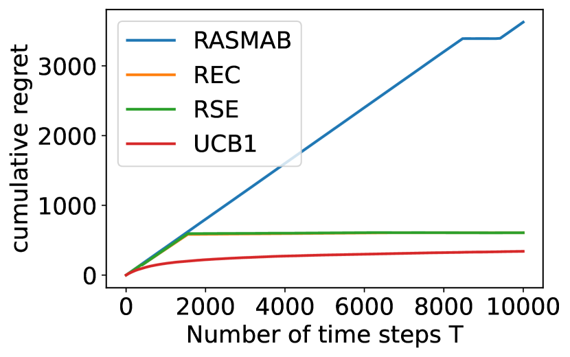
Model 1

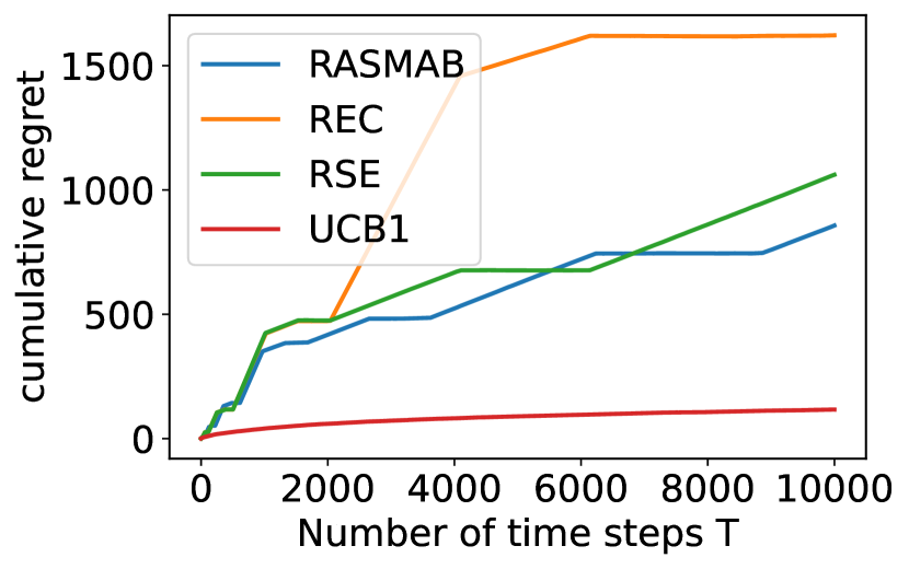
Model 2

Figure 1: Regret of algorithms. The horizontal axis indicates the number of rounds $t$ from $1$ to $T$, whereas the vertical axis indicates $\mathrm{Regret}(t)$. Results of REC and RSE in Model 1 are very similar.

We set the mean parameters as follows: $\bm{\mu}=(0.9,0.1,0.1,0.1,0.1,0.1,0.1,0.1,0.1,0.1)$ for Model 1 and $\bm{\mu}=(0.9,0.8,0.3)$ for Model 2. The amount of regret is depicted in Figure 1. A lower regret signifies superior performance. Being a nonreplicable algorithm, UCB1 naturally outperforms all other replicable algorithms for both cases.

In Model 1, with $\Delta_{K}/\Delta_{2}=1$, it favors REC and RSE because these algorithms can eliminate all arms simultaneously: REC and RSE not only outperform RASMAB but are also comparable to UCB1. This is consistent with our findings, which implies that the regret rates of these algorithms are identical to the regret rates of nonreplicable algorithms when $\log T=\Omega(\log(K(\log T)/\rho)/\rho^{2})$.

In Model 2, with a large $\Delta_{K}/\Delta_{2}=(0.9-0.3)/(0.9-0.8)=6$, it is more effective to eliminate arm $3$ (a clearly suboptimal arm) individually rather than all arms simultaneously. Therefore, RSE and RASMAB, which can eliminate each arm individually, outperform REC.

9 Related Work

Replicability was introduced by Impagliazzo et al. (2022) and they designed replicable algorithms for answering statistical queries, identifying heavy hitters, finding median, and learning halfspaces. Since then, replicable algorithms have been studied for bandit problems (Karbasi et al., 2023), reinforcement learning (Eaton et al., 2023), and clustering (Esfandiari et al., 2023b). The equivalence of various stability notions, including replicability and differential privacy (Dwork et al., 2014) was shown for a broad class of statistical problems (Bun et al., 2023). However, the equivalence therein does not necessarily guarantee an efficient conversion. Kalavasis et al. (2023) considered a relaxed notion of replicability. Note also that there are several relevant works Dixon et al. (2023); Chase et al. (2023) that study a different notion of replicability.

Stability in Sequential Learning

Stability has also been explored in the context of sequential learning. For example, robustness against corrupted distributions has been examined in the multi-armed bandit problem (Kim and Lim, 2016; Gajane et al., 2018; Kapoor et al., 2019; Basu et al., 2022). Differential privacy has also been considered in this context (Shariff and Sheffet, 2018; Basu et al., 2019; Hu and Hegde, 2022). Differential privacy considers the change of decision against the change of a single data point, whereas in the replicable bandits, we have more than one change of data points between two datasets that are generated from the identical data-generating process. Recent work (Dong and Yoshida, 2023) showed that an algorithm with a low average sensitivity (Varma and Yoshida, 2021) can be transformed to an online learning algorithm with low regret and inconsistency in the random-order setting, and hence in the stochastic setting.

Batched Bandit Problem

Prior to the introduction of the replicable bandit algorithm, the batched bandit problem was considered (Auer et al., 2002; Auer and Ortner, 2010; Cesa-Bianchi et al., 2013; Komiyama et al., 2013; Perchet et al., 2016; Gao et al., 2019; Esfandiari et al., 2021). In this problem, the algorithm needs to determine the sequence of draws at the beginning of each batch. Existing replicable bandit algorithms in Esfandiari et al. (2023a), as well as our algorithms, adopt phased approaches, and one can find similarities in the algorithmic design. Auer et al. (2002) proposed UCB2, which combines UCB with geometric size of the batches. Regarding the use of explore-then-commit strategy, Perchet et al. (2016) considered the two-armed batched bandit problem. They utilized the fact that the termination of the exploration phases in the explore-then-commit algorithm only occurs in a fixed number of rounds, a concept that we also utilize in the proof of our algorithms. However, their algorithm does not guarantee $\rho$-replicability for $\rho<1/2$. Our REC extends their results by introducing a randomized confidence level to guarantee a further level of replicability. Furthermore, our RSE generalizes both explore-then-commit and successive elimination (Gao et al., 2019; Esfandiari et al., 2023a) in a replicable way. Given $K,\rho$, for sufficiently large $T$, our algorithm’s performance is essentially similar to these batched algorithms Perchet et al. (2016); Gao et al. (2019). Note that, Esfandiari et al. (2023a) also briefly remarked the possibility of the use of the explore-then-commit strategy in replicable bandits.

10 Conclusion

We have examined multi-armed bandit algorithms that are $\rho$-replicable across various datasets generated from the same model. To ensure replicability, we introduced randomization to explore-then-commit and elimination algorithms. We demonstrated that the regret of these algorithms can be expressed as a sum of the standard bandit algorithm’s regret and the additional replicability-related regret. As these factors exhibit growth rates of $\Theta(\log T)$ and $o(\log T)$, respectively, for sufficiently large values of $T$, the replicability cost becomes negligible. This represents a significant improvement over existing algorithms. For our analysis, we have developed a framework based on decision variables, which can be used for bounding the probability of nonreplication in sequential replicable learning problems.

Appendix A Replicable Linear Successive Elimination

The Replicable Linear Successive Elimination (RLSE) algorithm is described in Algorithm 3.

Initialize the candidate set $\mathcal{A}_{1}=[K]$.
$p=1,2,\dots,P$ Draw shared random variables $U_{p,i}\sim\mathrm{Unif}(0,1)$ for each $i=0,1,2,\dots,K$.
Draw each arm $i$ for $\lceil N_{p}\pi^{*,\mathrm{app}}_{i}\rceil$ times.          $\rightarrow$ Approximated G-optimal exploration
$\mathcal{A}_{p+1}\leftarrow\mathcal{A}_{p}$.
$\hat{\Delta}(p)\geq(2+U_{p,0})\mathrm{Conf}^{\mathrm{max},a}({p})$ $\mathcal{A}_{p+1}=\{\operatorname*{arg\,max}_{i}\hat{\mu}_{i}(p)\}$.          $\rightarrow$ Eliminate all arms except for one. $i\in\mathcal{A}_{p+1}$ $\hat{\Delta}_{i}(p)\geq(2+U_{p,i})\mathrm{Conf}^{\mathrm{max},e}({p})$ $\mathcal{A}_{p+1}\leftarrow\mathcal{A}_{p+1}\setminus\{i\}$.          $\rightarrow$ Eliminate arm $i$.

Algorithm 3 Replicable Linear Successive Elimination (RLSE)

Appendix B Proofs on General Bound

Proof B.1 (Proof of Theorem 2).

Let $\mathcal{G}=\bigcap_{p}\mathcal{G}_{p}$. We have

$$\rho:=\mathbb{P}_{U,\mathcal{D}^{(1)},\mathcal{D}^{(2)}}\left[(I^{(1)}_{1},I^{(1)}_{2},\dots,I^{(1)}_{T})\neq(I^{(2)}_{1},I^{(2)}_{2},\dots,I^{(2)}_{T})\right]$$ (22)

$$\leq\mathbb{P}[(I^{(1)}_{1},I^{(1)}_{2},\dots,I^{(1)}_{T})\neq(I^{(2)}_{1},I^{(2)}_{2},\dots,I^{(2)}_{T}),\mathcal{G}^{(1)},\mathcal{G}^{(2)}]+\mathbb{P}_{\mathcal{D}^{(1)}}\left[\cup_{p}\mathcal{G}^{c}_{p}\right]+\mathbb{P}_{\mathcal{D}^{(2)}}\left[\cup_{p}\mathcal{G}^{c}_{p}\right]$$ (23)

$$\leq\mathbb{P}[(I^{(1)}_{1},I^{(1)}_{2},\dots,I^{(1)}_{T})\neq(I^{(2)}_{1},I^{(2)}_{2},\dots,I^{(2)}_{T}),\mathcal{G}^{(1)},\mathcal{G}^{(2)}]+2\sum_{p}\rho_{p}^{G}$$ (24)

    (by Definition 3.5) (25)

$$\leq\mathbb{P}\left[(d_{p}^{(1)})_{p=1}^{P}\neq(d_{p}^{(2)})_{p=1}^{P},\mathcal{G}^{(1)},\mathcal{G}^{(2)}\right]+2\sum_{p}\rho_{p}^{G}$$ (26)

    (by definition of decision variables) (27)

$$\leq\sum_{p}\mathbb{P}\left[d_{p}^{(1)}\neq d_{p}^{(2)},\cap_{p^{\prime}=1}^{p-1}\left\{d_{p^{\prime}}^{(1)}=d_{p^{\prime}}^{(2)}\right\},\mathcal{G}^{(1)},\mathcal{G}^{(2)}\right]+2\sum_{p}\rho_{p}^{G}$$ (28)

$$\leq\sum_{p}\mathbb{P}\left[d_{p}^{(1)}\neq d_{p}^{(2)},\cap_{p^{\prime}=1}^{p-1}\left\{d_{p^{\prime}}^{(1)}=d_{p^{\prime}}^{(2)},\mathcal{G}_{p^{\prime}}^{(1)},\mathcal{G}_{p^{\prime}}^{(2)}\right\},\mathcal{G}_{p}^{(1)},\mathcal{G}_{p}^{(2)}\right]+2\sum_{p}\rho_{p}^{G}$$ (29)

$$\leq\sum_{p}\mathbb{P}\left[d_{p}^{(1)}\neq d_{p}^{(2)}\,\biggl{|}\,\cap_{p^{\prime}=1}^{p-1}\left\{d_{p^{\prime}}^{(1)}=d_{p^{\prime}}^{(2)},\mathcal{G}_{p^{\prime}}^{(1)},\mathcal{G}_{p^{\prime}}^{(2)}\right\},\mathcal{G}_{p}^{(1)},\mathcal{G}_{p}^{(2)}\right]+2\sum_{p}\rho_{p}^{G}$$ (30)

$$\leq\sum_{p,i}\mathbb{P}\left[d_{p,i}^{(1)}\neq d_{p,i}^{(2)}\,\biggl{|}\,\cap_{p^{\prime}=1}^{p-1}\left\{d_{p^{\prime}}^{(1)}=d_{p^{\prime}}^{(2)},\mathcal{G}_{p^{\prime}}^{(1)},\mathcal{G}_{p^{\prime}}^{(2)}\right\},\mathcal{G}_{p}^{(1)},\mathcal{G}_{p}^{(2)}\right]+2\sum_{p}\rho_{p}^{G}$$ (31)

    (by union bound) (32)

$$=\sum_{p,i}\rho^{(p,i)}+2\sum_{p}\rho_{p}^{G}$$ (33)

$$\text{\ \ \ \ (by Definition \ref{def_nonrepr})}.$$ (34)

Appendix C Proofs on Algorithm 1

C.1 Stopping time

Let

$$p_{\mathrm{s}}=\min_{p}\left\{\mathrm{Conf}^{\mathrm{max}}({p})\leq\frac{10\Delta}{17}\right\}.$$

In the proof, we show that the algorithm is likely to break the loop at phase $p_{s}$ or $p_{s+1}$. Since $\mathrm{Conf}^{\mathrm{max}}({p})={\epsilon}_{p}\max\left(\sqrt{\log(KTP)},C_{\mathrm{mul}}\sqrt{\frac{\log(18K^{2}P/\rho)}{\rho^{2}}}\right)$, we can see that

$$N_{p_{s}}\leq 8a^{2}\sigma^{2}\left(\frac{17}{10\Delta}\right)^{2}\left(\log(KTP)+(C_{\mathrm{mul}})^{2}\frac{\log(18K^{2}P/\rho)}{\rho^{2}}\right).$$ (35)

C.2 Replicability of Algorithm 1

This section bounds the probability of nonreplication of Theorem 3. We use the general bound of Section 3. Let the good event (Definition 3.5) be

$$\mathcal{G} =\bigcap_{p\in[P]}\mathcal{G}_{p}$$ (36)

$$\mathcal{G}_{p} =\bigcap_{i,j\in[K]}\left\{|\Delta_{ij}-\hat{\Delta}_{ij}(p)|\leq\rho\mathrm{Conf}^{\mathrm{repr}}({p})\right\}.$$ (37)

Event $\mathcal{G}$ states that all estimators lie in a region that is $\rho$ times smaller than $\mathrm{Conf}^{\mathrm{repr}}({p})$.

Lemma 9.

Event $\mathcal{G}$ holds with probability at least $1-\rho/18$.

It is easy to see that the only decision variable at phase $p$ is

$$d_{(p,0)}:=\mathbf{1}\left[\hat{\Delta}(p)\geq(2+U_{p})\mathrm{Conf}^{\mathrm{max}}({p})\right].$$

Lemma 10.

Under $\mathcal{G}$, the probability of nonreplication is $\rho^{(p,0)}=0$ for any $p\neq p_{\mathrm{s}}$.

Lemma 10 states that the only effective decision variable is that of phase $p_{\mathrm{s}}$.

Lemma 11.

Under $\mathcal{G}$, the probability of nonreplication at each decision point is at most $\rho^{(p,0)}=8\rho/9$ for $p=p_{\mathrm{s}}$.

Proof C.1 (Proof of nonreplicability part of Theorem 3).

Theorem 2 and Lemmas 9–11 imply that the probability of misidentification is at most $2\times\rho/18+8\rho/9=\rho$, which completes the proof.

In the following, we derive Lemmas 9–11.

Proof C.2 (Proof of Lemma 9).

Since $\Delta_{ij}=\mu_{i}-\mu_{j}$, $\hat{\Delta}_{ij}-\Delta_{ij}$ is estimating the sum of two $\sigma$-subgaussian random variables, which is a $2\sigma$-subgaussian random variable. By using Lemma 1 and taking a union bound over all possible $K(K-1)/2$ pairs of $ij$ and phases $1,\dots,P$, Event $\mathcal{G}$ holds with high probability:

$$\mathbb{P}[\mathcal{G}] \geq 1-K(K-1)P\exp\left(-\frac{(\rho\mathrm{Conf}^{\mathrm{repr}}({p}))^{2}N_{p}}{8\sigma^{2}}\right)$$ (38)

$$\geq 1-K(K-1)P\exp\left(-\log(18K^{2}P/\rho)\right)\text{\ \ \ \ (by definition of $N_{p},\mathrm{Conf}^{\mathrm{repr}}({p})$)}$$ (39)

$$\geq 1-K(K-1)P\times\frac{\rho}{18K^{2}P}\geq 1-\frac{\rho}{18},$$ (40)

which completes the proof.

Proof C.3 (Proof of Lemma 10).

First, we show that there are at most $2$ phases where the break from the loop (i.e., $\min_{p}d_{(p,1)}=1$) occurs. We first show that a break never occurs if $p<p_{s}$, which implies

$$\Delta<\frac{17}{10}\mathrm{Conf}^{\mathrm{max}}({p}),$$

and thus

$$\hat{\Delta}(p) \leq\Delta+\rho\mathrm{Conf}^{\mathrm{repr}}({p})\text{\ \ \ \ (by $\mathcal{G}$)}$$ (41)

$$\leq\Delta+\frac{\rho}{C_{\mathrm{mul}}}\mathrm{Conf}^{\mathrm{max}}({p})$$ (42)

$$\leq\Delta+\frac{4\rho}{9}\mathrm{Conf}^{\mathrm{max}}({p})$$ (43)

$$\leq(\frac{17}{10}+\frac{4\rho}{9})\mathrm{Conf}^{\mathrm{max}}({p})$$ (44)

$$\leq 2\mathrm{Conf}^{\mathrm{max}}({p})\text{\ \ \ \ (by $\rho\leq 1/2$)}$$ (45)

$$\leq(2+U_{p})\mathrm{Conf}^{\mathrm{max}}({p}).$$ (46)

We next show that $p=p_{s}+1$, which implies

$$\Delta\geq\frac{17}{5}{\epsilon}_{p}\mathrm{Conf}^{\mathrm{max}}({p}).$$

implies a break, because

$$\hat{\Delta}(p) \geq\Delta-\rho\mathrm{Conf}^{\mathrm{repr}}({p})\text{\ \ \ (by $\mathcal{G}$)}$$ (47)

$$\geq\Delta-\frac{\rho}{C_{\mathrm{mul}}}\mathrm{Conf}^{\mathrm{max}}({p})$$ (48)

$$\geq\frac{17}{5}\mathrm{Conf}^{\mathrm{max}}({p})-\frac{4\rho}{9}\mathrm{Conf}^{\mathrm{max}}({p})$$ (49)

$$\geq 3\mathrm{Conf}^{\mathrm{max}}({p})\text{\ \ \ (by $\rho\leq 1/2$)}$$ (50)

$$\geq(2+U_{p})\mathrm{Conf}^{\mathrm{max}}({p}).$$ (51)

The above results, combined with the fact that ${\epsilon}_{p}$ is halved at each phase, implying that the only decision points where the decision variable can take both of $\{0,1\}$ are $p_{\mathrm{s}},p_{\mathrm{s}}+1$. Therefore, if the decision variable at phase $p_{\mathrm{s}}$ matches, the decision variable at $p_{\mathrm{s}}+1$ and subsequent match.

Proof C.4 (Proof of Lemma 11).

For phase $p_{s}$, we bound the probability of nonreplication. At the end of phase $p=p_{s}$, it utilizes the randomness $U_{p}\sim\mathrm{Unif}(0,1)$, and the random variable $(2+U_{p})\mathrm{Conf}^{\mathrm{max}}({p})$ is uniformly distributed on a region of size $\mathrm{Conf}^{\mathrm{max}}({p})$. Meanwhile, event $\mathcal{G}$ implies

$$\left|\left(\hat{\Delta}^{(1)}(p)-(2+U_{p})\mathrm{Conf}^{\mathrm{max}}({p})\right)-\left(\hat{\Delta}^{(2)}(p)-(2+U_{p})\mathrm{Conf}^{\mathrm{max}}({p})\right)\right|\leq 2\rho\mathrm{Conf}^{\mathrm{repr}}({p}).$$ (52)

This implication suggests that within a region of at most width $2\rho\mathrm{Conf}^{\mathrm{repr}}({p})$, the expressions $\left(\hat{\Delta}^{(1)}(p)-(2+U_{p})\mathrm{Conf}^{\mathrm{max}}({p})\right)$ and $\left(\hat{\Delta}^{(2)}(p)-(2+U_{p})\mathrm{Conf}^{\mathrm{max}}({p})\right)$ can have different signs. Therefore, the probability of nonreplication is at most

$$\frac{2\rho\mathrm{Conf}^{\mathrm{repr}}({p})}{\mathrm{Conf}^{\mathrm{max}}({p})}\leq 8\rho/9,$$

where the last inequality follows from the assumption $C_{\mathrm{mul}}\geq 9/4$.

C.3 Regret Bound of Algorithm 1

This section derives the regret bound in Theorem 3. We prepare the following events:

$$\mathcal{G}^{\mathrm{reg}} =\bigcap_{p\in[P]}\mathcal{G}^{\mathrm{reg}}_{p}$$ (53)

$$\mathcal{G}^{\mathrm{reg}}_{p} =\bigcap_{i,j\in[K]}\left\{|\Delta_{ij}-\hat{\Delta}_{ij}(p)|\leq\mathrm{Conf}^{\mathrm{reg}}({p})\right\}.$$ (54)

Event $\mathcal{G}^{\mathrm{reg}}$ states that all estimators lie in the confidence region. The following theorem bounds the probability such that event $\mathcal{G}^{\mathrm{reg}}$ occurs.

Lemma 12.

$$\mathbb{P}[\mathcal{G}^{\mathrm{reg}}]\geq 1-\frac{K}{T}.$$

Proof C.5 (Proof of Lemma 12).

The proof follows similar steps as Lemma 9. By using Lemma 1 and taking a union bound over all possible $K(K-1)/2$ pairs of $ij$ and phases $1,\dots,P$, Event $\mathcal{G}^{\mathrm{reg}}$ holds with high probability:

$$\mathbb{P}[\mathcal{G}^{\mathrm{reg}}] \geq 1-K(K-1)P\exp\left(-\frac{(\mathrm{Conf}^{\mathrm{reg}}({p}))^{2}N_{p}}{8\sigma^{2}}\right)$$ (55)

$$\geq 1-K(K-1)P\exp\left(-\log(KPT)\right)\text{\ \ \ \ (by definition of $N_{p}$, $\mathrm{Conf}^{\mathrm{reg}}({p})$)}$$ (56)

$$\geq 1-K(K-1)P\times\frac{1}{KPT}\geq 1-\frac{K}{T},$$ (57)

which completes the proof.

Assume that $\mathcal{G}^{\mathrm{reg}}$ holds. The following shows that the break occurs by the end of phase $p_{\mathrm{s}}+2$.

$$\hat{\Delta}(p_{\mathrm{s}}+2) \geq\Delta-2\mathrm{Conf}^{\mathrm{reg}}({p_{\mathrm{s}}+2})\text{\ \ \ \ (by $\mathcal{G}^{\mathrm{reg}}$)}$$ (58)

$$\geq\Delta-2\mathrm{Conf}^{\mathrm{max}}({p_{\mathrm{s}}+2})$$ (59)

$$\geq\frac{34}{5}\mathrm{Conf}^{\mathrm{max}}({p_{\mathrm{s}}+2})-2\mathrm{Conf}^{\mathrm{max}}({p_{\mathrm{s}}+2})\text{\ \ \ \ (by definition of $p_{\mathrm{s}}$)}$$ (60)

$$\geq 3\mathrm{Conf}^{\mathrm{max}}({p})\geq(2+U_{p})\mathrm{Conf}^{\mathrm{max}}({p}).$$ (61)

The regret up to this phase is at most

$$\sum_{i}\Delta_{i}\times N_{p_{\mathrm{s}}+2}.$$

We have

$$N_{p_{\mathrm{s}}+2} =O\left(\log T\times a^{2(p_{\mathrm{s}}+2)}\right)$$ (62)

$$=O\left(\log T\times a^{2p_{\mathrm{s}}}\right)$$ (63)

$$=O\left(\left(\frac{1}{\Delta}\right)^{2}\max\left(\log(KTP)+\frac{\log(KP/\rho)}{\rho^{2}}\right)\right).\text{\ \ \ \ (by equation~{}\ref{ineq_npstop})}$$ (64)

Moreover, assume that $\hat{\mu}_{i}(p)\geq\hat{\mu}_{1}(p)$ when a break occurs at phase $p$. Then,

$$\hat{\mu}_{i}(p)-\hat{\mu}_{1}(p) \geq(2+U_{p})\mathrm{Conf}^{\mathrm{max}}({p})\text{\ \ \ \ (by the fact that break occurs)}$$ (65)

$$>2\mathrm{Conf}^{\mathrm{max}}({p})$$ (66)

$$>2\mathrm{Conf}^{\mathrm{reg}}({p}).$$ (67)

Meanwhile, $\mathcal{G}^{\mathrm{reg}}$ implies for all phase $p$

$$\hat{\mu}_{i}(p)-\hat{\mu}_{1}(p)\leq 2\mathrm{Conf}^{\mathrm{reg}}({p}),$$ (68)

which implies  equation 67 never occurs. By proof of contradiction. $\hat{\mu}_{1}(p)>\hat{\mu}_{i}(p)$. Therefore, the empirically best arm is always the true best arm, and we have zero regret during the exploitation period under $\mathcal{G}^{\mathrm{reg}}$. In summary,

$$\mathbb{E}[\mathrm{Regret}(T)] \leq\mathbb{E}[\mathbf{1}[\mathcal{G}^{\mathrm{reg}}]\cdot\mathrm{Regret}(T)]+O(1)$$ (69)

    (equation 55 implies $$\Pr[(\mathcal{G}^{\mathrm{reg}})^{c}] K/T=O(1/T)$$ is ) (70)

$$\leq\underbrace{O\left(\sum_{i}\Delta_{i}N_{p_{s}+2}\right)}_{\text{Regret during exploration}}+\underbrace{0}_{\text{Regret during exploitation}}+\underbrace{O(1)}_{\text{Regret in the case of $(\mathcal{G}^{\mathrm{reg}})^{c}$}}$$ (71)

$$\leq O\left(\sum_{i}\frac{\Delta_{i}}{\Delta^{2}}\max\left(\log(KTP)+\frac{\log(KP/\rho)}{\rho^{2}}\right)\right),$$ (72)

which, combined with $P=O(\log T)$, completes the proof.

Appendix D Proofs on Algorithm 2

D.1 Replicability of Algorithm 2

Similarly to that of Theorem 3, we define the good event. Let the good event (Definition 3.5) be

$$\mathcal{G} =\bigcap_{p\in[P]}(\mathcal{G}_{p,0}\cap\bigcap_{i\in[K]}\mathcal{G}_{p,i})$$ (73)

$$\mathcal{G}_{a,0} =\bigcap_{i,j\in[K]}\left\{|\Delta_{ij}-\hat{\Delta}_{ij}(p)|\leq\rho_{a}\mathrm{Conf}^{\mathrm{repr},a}({p})\right\}$$ (74)

$$\mathcal{G}_{a,i} =\bigcap_{i,j\in[K]}\left\{|\Delta_{ij}-\hat{\Delta}_{ij}(p)|\leq\rho_{e}\mathrm{Conf}^{\mathrm{repr},e}({p})\right\}.$$ (75)

Lemma 13.

Event $\mathcal{G}$ holds with probability at least $1-\rho/18$. Moreover, under $\mathcal{G}$, arm $1$ (= best arm) is never eliminated (i.e., $1\in\mathcal{A}_{p}$ for all $p$).

There are $K+1$ binary decision variables at phase $p$. The first decision variable is

$$d_{(p,0)} :=\mathbf{1}\left[\hat{\Delta}(p)>(2+U_{p,0})\mathrm{Conf}^{\mathrm{max},a}({p})\right].$$ (76)

The other $K$ decision variables are

$$d_{(p,i)} :=\mathbf{1}\left[\hat{\Delta}_{i}(p)>(2+U_{p,i})\mathrm{Conf}^{\mathrm{max},e}({p})\right]$$ (77)

for each $i=1,2,\dots,K$. If all decision variables are identical between two runs then the sequence of draws is identical between them.

Lemma 14.

Let

$$p_{\mathrm{s},0}=\min_{p}\left\{\mathrm{Conf}^{\mathrm{max},a}({p})\leq\frac{10\Delta}{17}\right\}.$$

Under $\mathcal{G}$, we have $\rho^{(p,0)}=0$ for any $p\neq p_{\mathrm{s},0}$.

Lemma 15.

Let

$$p_{\mathrm{s},i}=\min_{p}\left\{\mathrm{Conf}^{\mathrm{max},e}({p})\leq\frac{10\Delta_{i}}{17}\right\},$$

for each $i\in[K]$. Then, $\rho^{(p,i)}=0$ for all $p\neq p_{\mathrm{s},i}$.

Lemma 16.

Under $\mathcal{G}$, the probability of nonreplication at each decision point is at most $\rho^{(p,0)}=8\rho_{a}/9$ or $\rho^{(p,i)}=8\rho_{e}/9$ for $i\in\{2,\dots,K\}$.

Proof D.1 (Proof of nonreplicability part of Theorem 4).

Theorem 2 and Lemmas 13–16 imply that the probability of misidentification is at most $(\rho_{a}+(K-1)\rho_{e})\times(2\times\frac{1}{18}+\frac{8}{9})=\rho$, which completes the proof.

Proof D.2 (Proof of Lemma 13).

By using essentially the same discussion as Lemma 9 yields the fact that event $\mathcal{G}$ holds with probability at least $1-\rho/18$.

In the following, we show that arm $1$ is never eliminated under $\mathcal{G}$. Elimination of arm $1$ at phase $p$ due to $\rho_{a}$ implies that there exists a suboptimal arm $i\neq 1$ such that

$$\hat{\mu}_{i}(p)-\mu_{1}(p)\geq(2+U_{p,0})\mathrm{Conf}^{\mathrm{max},a}({p})\geq 2\mathrm{Conf}^{\mathrm{max},a}({p}),$$ (78)

which never occurs under $\mathcal{G}$, since $\mathcal{G}$ implies

$$|\mu_{1}-\hat{\mu}_{1}(p)|,|\mu_{i}-\hat{\mu}_{i}(p)|<\mathrm{Conf}^{\mathrm{repr},a}({p})\leq\mathrm{Conf}^{\mathrm{max},a}({p})$$

and thus

$$\hat{\mu}_{i}(p)-\mu_{1}(p)<2\mathrm{Conf}^{\mathrm{max},a}({p})+\mu_{i}-\mu_{1}\leq 2\mathrm{Conf}^{\mathrm{max},a}({p}),$$ (79)

which contradicts equation 78. The same discussion goes for the elimination due to $\rho_{e}$.

Proof D.3 (Proof of Lemma 14).

Given arm $1$ is never eliminated in $\mathcal{A}_{p_{\mathrm{s},0}+1}$ unless $d_{(p,0)}=1$ occurs, the minimum gap $\Delta=\mu_{1}-\mu_{2}$ is the same as the minimum gap among $\mathcal{A}_{p_{\mathrm{s},0}+1}$. The rest of this Lemma, which shows $d_{(p,0)}=1$ for the first phase at $p=p_{\mathrm{s},0}$ or $p_{\mathrm{s},0}+1$, is very similar to that of Lemma 10, and thus we omit it. The only non-zero decision variable is $\rho^{(p,0)}$ at $p=p_{\mathrm{s},0}$ by using the same discussion.

Proof D.4 (Proof of Lemma 15).

We omit the proof because it is very similar to Lemma 10.

Proof D.5 (Proof of Lemma 16).

We omit the proof because the proof for each $i=0,1,2,\dots,K$ is very similar to Lemma 11.

D.2 Regret Bound of Algorithm 2

We prepare the following events:

$$\mathcal{G}^{\mathrm{reg}} =\bigcap_{p\in[P]}\mathcal{G}^{\mathrm{reg}}_{p}$$ (80)

$$\mathcal{G}^{\mathrm{reg}}_{p} =\bigcap_{i,j\in[K]}\left\{|\Delta_{ij}-\hat{\Delta}_{ij}(p)|\leq\mathrm{Conf}^{\mathrm{reg}}({p})\right\}.$$ (81)

Event $\mathcal{G}^{\mathrm{reg}}$ states that all estimators lie in the confidence region.

(A) The $O(K)$ regret bound: This part is very identical to that of Algorithm 1 because, under $\mathcal{G}^{\mathrm{reg}}$, all but arm $1$ is eliminated by phase $p_{\mathrm{s},0}+2$. We omit the proof to avoid repetition.

(B) The other two regret bounds: We first derive the distribution-dependent bound. We show that under $\mathcal{G}^{\mathrm{reg}}$, each arm $i$ is eliminated by phase $p_{\mathrm{s},i}+2$. Assume that $\mathcal{G}^{\mathrm{reg}}$ holds. The following shows that the break occurs by the end of phase $p_{\mathrm{s},i}+2$.

$$\hat{\mu}_{i}(p_{\mathrm{s},i}+2)-\hat{\mu}_{1}(p_{\mathrm{s},i}+2) \geq\Delta_{i}-2\mathrm{Conf}^{\mathrm{reg}}({p_{\mathrm{s},i}+2})\text{\ \ \ \ (by $\mathcal{G}^{\mathrm{reg}}$)}$$ (82)

$$\geq\Delta_{i}-2\mathrm{Conf}^{\mathrm{max},e}({p_{\mathrm{s},i}+2})$$ (83)

$$\geq\frac{34}{5}\mathrm{Conf}^{\mathrm{max},e}({p_{\mathrm{s},i}+2})-2\mathrm{Conf}^{\mathrm{max},e}({p_{\mathrm{s},i}+2})\text{\ \ \ \ (by definition of $p_{\mathrm{s},i}$)}$$ (84)

$$\geq 3\mathrm{Conf}^{\mathrm{max},e}({p})\geq(2+U_{p})\mathrm{Conf}^{\mathrm{max}}({p}).$$ (85)

Therefore, each arm $i$ is drawn at most

$$N_{i,\mathrm{max}} :=O\left(4^{p_{\mathrm{s},i}+2}\log T\right)$$ (86)

$$=O\left(\frac{1}{\Delta_{i}^{2}}\left(\log(KTP)+\frac{\log(KP/\rho_{e})}{(\rho_{e})^{2}}\right)\right)$$ (87)

$$=O\left(\frac{1}{\Delta_{i}^{2}}\left(\log(KTP)+\frac{K^{2}\log(KP/\rho)}{\rho^{2}}\right)\right)$$ (88)

times, and thus regret is bounded as

$$\mathbb{E}[\mathrm{Regret}(T)] \leq\mathbb{E}[\mathbf{1}[\mathcal{G}^{\mathrm{reg}}]\cdot\mathrm{Regret}(T)]+O(1)$$ (89)

$$\leq\underbrace{\sum_{i}\Delta_{i}N_{i,\mathrm{max}}}_{\text{Regret during exploration}}+\underbrace{0}_{\text{Regret during exploitation, which is $0$ by Lemma \ref{lem_good_rse}}}+\underbrace{O(1)}_{\text{Regret in the case of $(\mathcal{G}^{\mathrm{reg}})^{c}$}}$$ (90)

$$\leq O\left(\sum_{i}\frac{1}{\Delta_{i}}\left(\log(KTP)+\frac{K^{2}\log(KP/\rho)}{\rho^{2}}\right)\right)$$ (91)

$$\leq O\left(\sum_{i}\frac{1}{\Delta_{i}}\left((\log T)+\frac{K^{2}\log(K(\log T)/\rho)}{\rho^{2}}\right)\right),$$ (92)

which is the second regret bound of Theorem 4.

We finally derive the distribution-independent regret bound. Letting $N_{i}(T)$ be the number of draws of arm $i$ in the $T$ rounds, we have

$$\mathrm{Regret}(T)\mathbf{1}[\mathcal{G}^{\mathrm{reg}}] \leq\sum_{i}\Delta_{i}N_{i}(T)+O(1)$$ (93)

$$=\sum_{i}\Delta_{i}\sqrt{N_{i,\mathrm{max}}}\sqrt{N_{i}(T)}+O(1),$$ (94)

and

$$\sum_{i}\Delta_{i}\sqrt{N_{i,\mathrm{max}}}\sqrt{N_{i}(T)} \leq O(1)\times\sum_{i}\Delta_{i}\sqrt{\frac{1}{\Delta_{i}^{2}}\left((\log T)+\frac{K^{2}\log(K(\log T)/\rho)}{\rho}\right)}\sqrt{N_{i}(T)}$$ (95)

      (by equation 88) (96)

$$\leq O(1)\times\sum_{i}\sqrt{(\log T)+\frac{K^{2}\log(K(\log T)/\rho)}{\rho}}\sqrt{N_{i}(T)}$$ (97)

$$\leq O(1)\times\sqrt{(\log T)+\frac{K^{2}\log(K(\log T)/\rho)}{\rho}}\sqrt{KT}$$ (98)

$$\text{\ \ \ \ (by Cauchy-Schwarz and $\sum_{i}N_{i}(T)=T$)},$$ (99)

and thus

$$\mathbb{E}[\mathrm{Regret}(T)] \leq\mathbb{E}[\mathrm{Regret}(T)\mathbf{1}[\mathcal{G}^{\mathrm{reg}}]]+O(1)$$ (100)

$$=O\left(\sqrt{KT\left((\log T)+\frac{K^{2}\log(K(\log T)/\rho)}{\rho}\right)}\right),$$ (101)

which is the third regret bound of Theorem 4.

Appendix E Proofs on the Lower Bound

In the following, we derive Theorem 5. The proof is inspired by Theorem 7.2 of Impagliazzo et al. (2022) but is significantly more challenging due to the adaptiveness of sampling. In particular, Lemma 17 utilizes the change-of-measure argument and works even if the number of draws $N_{2}(T)$ on arm $2$ is a random variable.

Proof E.1 (Proof of Theorem 5).

The goal of the proof here is to derive the inequality:

$$\mathbb{E}[\mathrm{Regret}(T)]=\Omega\left(\frac{1}{\rho^{2}\Delta\log((\rho\Delta)^{-1})}\right).$$ (102)

We consider the set of models $\mathcal{P}$, where $\mu_{1}=1/2$ is fixed and $\mu_{2}\in[1/2-\Delta,1/2+\Delta]$. With a slight abuse of notation, we specify a model in $\mathcal{P}$ by $\mu_{2}-1/2$. We also denote $U$ to the internal randomness. For example,

$$\mathbb{P}_{-\Delta,U}[\mathcal{X}]$$

be the probability that event $\mathcal{X}$ occurs under the corresponding model $(\mu_{1},\mu_{2})=(1/2,1/2-\Delta)$ and randomness $U$.

Markov’s inequality on the regret and the assumption of uniformly goodness implies that, there exists a sublinear function $R(T)$ such that, at least 3/4 of the choice of the randomness $U$, we have $\mathbb{E}_{-\Delta,U}[\mathrm{Regret}(T)]\leq R(T)$. Similarly, at least 3/4 of the choice of the randomness $U$, we have $\mathbb{E}_{\Delta,U}[\mathrm{Regret}(T)]\leq R(T)$. By taking a union bound, at least half ($=1-(1/4+1/4)$) over the choice of $U$, we have

$$\max\{\mathbb{E}_{-\Delta,U}[\mathrm{Regret}(T)],\mathbb{E}_{\Delta,U}[\mathrm{Regret}(T)]\}\leq R(T).$$ (103)

Let $T_{0}$ be such that

$$\forall\,T\geq T_{0}\ R(T)\leq\frac{T\Delta}{8}.$$ (104)

In the following, we consider an arbitrary $T\geq T_{0}$. In parts (A) and (B), we fix $U$ such that equation 103 holds. Part (C) marginalizes it over $U$.

(A) Fix the randomness $U$ and consider behavior of algorithm for different models:

Let $N_{C}(U)$ be the smallest among the integer $n$ such that

$$\mathbb{P}_{-\Delta,U}\left[N_{2}(T)\geq n\right] \leq\frac{1}{4}\text{\ and}$$ (105)

$$\mathbb{P}_{\Delta,U}\left[N_{2}(T)\geq n\right] \geq\frac{3}{4}.$$ (106)

At least one such an integer exists; $n=T/2$ satisfies this condition because otherwise

$$\max\{\mathbb{E}_{-\Delta,U}[\mathrm{Regret}(T)],\mathbb{E}_{\Delta,U}[\mathrm{Regret}(T)]\}$$ (107)

$$\geq\max\left\{\mathbb{P}_{-\Delta,U}\left[N_{2}(T)\geq\frac{T}{2}\right]\frac{T\Delta}{2},\left(1-\mathbb{P}_{\Delta,U}\left[N_{2}(T)\geq\frac{T}{2}\right]\right)\frac{T\Delta}{2}\right\}$$ (108)

$$>\frac{T\Delta}{8}$$ (109)

$$\text{\ \ \ \ \ \ (by $\mathbb{P}_{-\Delta,U}\left[N_{2}(T)\geq\frac{T}{2}\right]>\frac{1}{4}$ or $\mathbb{P}_{\Delta,U}\left[N_{2}(T)\geq\frac{T}{2}\right]<\frac{3}{4}$)},$$ (110)

which violates equation 104.

By continuity, there exists $\nu=\nu(U)\in(-\Delta,+\Delta)$ such that $\mathbb{P}_{\nu,U}[N_{2}(T)\geq N_{C}(U)]=1/2$. By Lemma 17, there exists $C_{I}=\Theta(1)$ such that, for any $\nu^{\prime}\in[\nu-C_{I}/\sqrt{\log(N_{C}(U))N_{C}(U)},\nu+C_{I}/\sqrt{\log(N_{C}(U))N_{C}(U)}]=:\mathcal{I}(U)$ we have $\mathbb{P}_{\nu^{\prime},U}[N_{2}(T)\geq N_{C}(U)]\in(1/3,2/3)$.

(B) Marginalize it over models: Assume that we first draw a model uniformly random from $[-\Delta,\Delta]$, and then run the algorithm. Conditioned on the shared randomness $U$, with probability at least $C_{I}/(\sqrt{\log(N_{C}(U))N_{C}(U)}\Delta)$, we draw model in $\mathcal{I}(U)$. For a model in $\mathcal{I}(U)$, there is $2\times(1/3)\times(2/3)=4/9$ probability of nonreplicability.

(C) Marginalize it over shared random variable $U$: equation 103 implies that the discussions in (A) and (B) hold at least half of the random variable $U$. We let the set of such random variables as $\mathcal{U}_{half}$. Let

$$n_{c}=\frac{\int_{U\in\mathcal{U}_{half}}N_{C}(U)dP(U)}{\int_{U\in\mathcal{U}_{half}}dP(U)}$$

be the expected value of $N_{C}(U)$ marginalized over the distribution on $\mathcal{U}_{half}$. We have

$$\frac{1}{2}\times\frac{4}{9}\frac{C_{I}}{\sqrt{\log(n_{c})n_{c}}\Delta}$$ (111)

$$\leq\int_{U\in\mathcal{U}_{half}}\frac{4}{9}\frac{C_{I}}{\sqrt{\log(n_{c})n_{c}}\Delta}dP(U)$$ (112)

    (by at least half of $$U \mathcal{U}_{half}$$ are in ) (113)

$$\leq\int_{U\in\mathcal{U}_{half}}\frac{4}{9}\frac{C_{I}}{\sqrt{\log(N_{C}(U))N_{C}(U)}\Delta}dP(U)$$ (114)

    (by convexity of $$f(x):=1/\sqrt{x\log x} f(\mathbb{E}[x])\leq\mathbb{E}[f(x)]$$ and Jensen’s inequality ) (115)

$$\leq\rho$$ (116)

$$\text{\ \ \ \ (by part (B) and $\rho$-replicability)},$$ (117)

which implies

$$n_{c}=\Omega\left(\frac{1}{(\rho\Delta)^{2}\log((\rho\Delta)^{-1})}\right).$$ (118)

The regret is lower-bounded as

$$\max\{\mathbb{E}_{-\Delta}[\mathrm{Regret}(T)],\mathbb{E}_{\Delta}[\mathrm{Regret}(T)]\}$$ (119)

$$\geq\max\left\{\mathbb{P}_{-\Delta}[N_{2}(T)\geq n_{c}-1]\Delta(n_{c}-1),\left(1-\mathbb{P}_{\Delta}[N_{2}(T)\geq n_{c}-1]\right)\Delta(T-n_{c}+1)\right\}$$ (120)

$$\geq\max\left\{\mathbb{P}_{-\Delta}[N_{2}(T)\geq n_{c}-1]\Delta(n_{c}-1),\left(1-\mathbb{P}_{\Delta}[N_{2}(T)\geq n_{c}-1]\right)\Delta\left(\frac{T}{2}+1\right)\right\}$$ (121)

      (by $$n_{c}\leq T/2$$) (122)

$$\geq\frac{1}{4}\times\Delta(n_{c}-1)$$ (123)

      (by $$N_{C}(U)-1 n_{c}\leq T/2$$ violates equation 105 or equation 106, and ) (124)

$$=\Omega\left(\frac{1}{\rho^{2}\Delta\log((\rho\Delta)^{-1})}\right).\text{\ \ \ \ (by equation~{}\ref{ineq_ncbound})}$$ (125)

Remark E.2.

(Extension for $K$-armed Lower Bound) Here, equation 119 bounds at least one of two quantities $\mathbb{E}_{-\Delta}[\mathrm{Regret}(T)]$ or $\mathbb{E}_{\Delta}[\mathrm{Regret}(T)]$. If we can directly bound $\mathbb{E}_{-\Delta}[\mathrm{Regret}(T)]$, then we should be able to extend the results here to the $K$-armed case.

E.1 Lemmas for Regret Lower Bound

The following lemma is used to bound the gradient of the probability of occurrences. This lemma corresponds to the derivative of the acceptance function of Lemma 7.2 in Impagliazzo et al. (2022), but more technical due to the fact that $N_{2}(T)$ is a random variable.

Lemma 17.

(Likelihood ratio) Let

$$\mathcal{E}=\{N_{2}(T)\leq N_{C}\}$$ (126)

and $\nu$ be such that $\mathbb{P}_{\nu,U}[\mathcal{E}]=1/2$. There exists a value $C_{I}=\Theta(1)$ that does not depend on the shared random variable $U$ such that, for any model $\nu^{\prime}\in[\nu-C_{I}/\sqrt{\log(N_{C})N_{C}},\nu+C_{I}/\sqrt{\log(N_{C})N_{C}}]$, we have

$$\mathbb{P}_{\nu^{\prime},U}[\mathcal{E}]\in\left(\frac{1}{3},\frac{2}{3}\right).$$ (127)

Proof E.3 (Proof of Lemma 17).

In the following, we bound $\mathbb{P}_{\nu^{\prime},U}[\mathcal{E}]$ by using the change-of-measure argument.

Let the log-likelihood ratio between from models $\nu,\nu^{\prime}$ be

$$L_{t} =\sum_{n=1}^{N_{2}(t)}\log\left(\frac{X_{2,n}\left(\frac{1}{2}+\nu\right)+(1-X_{2,n})\left(\frac{1}{2}-\nu\right)}{X_{2,n}\left(\frac{1}{2}+\nu^{\prime}\right)+(1-X_{2,n})\left(\frac{1}{2}-\nu^{\prime}\right)}\right),$$ (128)

where $X_{2,n}$ is the $n$-th reward from arm $2$ and $N_{2}(t)$ be the number of draws on arm $2$ during the first $t$ rounds.

We have

$$\mathbb{P}_{\nu^{\prime},U}[\mathcal{E}] =\mathbb{E}_{\nu,U}\left[\mathbf{1}[\mathcal{E}]e^{-L_{T}}\right].\text{\ \ \ \ (change-of-measure)}$$ (129)

Note that, under $\nu$ the random variable

$$\log\left(\frac{X_{2,n}\left(\frac{1}{2}+\nu\right)+(1-X_{2,n})\left(\frac{1}{2}-\nu\right)}{X_{2,n}\left(\frac{1}{2}+\nu^{\prime}\right)+(1-X_{2,n})\left(\frac{1}{2}-\nu^{\prime}\right)}\right)$$

is mean $d_{\mathrm{KL}}(\nu,\nu^{\prime})$ and bounded by

$$R=\left|\log\left(\frac{2+\nu}{2+\nu^{\prime}}\right),\log\left(\frac{2-\nu}{2-\nu^{\prime}}\right)\right|=O(|\nu-\nu^{\prime}|)=O\left(\frac{C_{I}}{\sqrt{\log(N_{C})N_{C}}}\right).$$

Under $\mathcal{E}$, $N_{2}(T)\leq N_{C}$ and $L_{T}$ is bounded as the max of random variables

$$L_{T}\leq\max_{N\leq N_{C}}\left(\sum_{n\leq N}Z_{n}\right),$$

where

$$Z_{n}:=\log\left(\frac{X_{2,n}\left(\frac{1}{2}+\nu\right)+(1-X_{2,n})\left(\frac{1}{2}-\nu\right)}{X_{2,n}\left(\frac{1}{2}+\nu^{\prime}\right)+(1-X_{2,n})\left(\frac{1}{2}-\nu^{\prime}\right)}\right)$$

is a random variable with its mean $d_{\mathrm{KL}}(\nu,\nu^{\prime})$ and radius $R$. Hoeffding inequality and union bound over $N=1,2,\dots,N_{C}$ implies that, with probability at least $1-1/12$ we have

$$|L_{T}| \leq N_{C}d_{\mathrm{KL}}(1/2+\nu,1/2+\nu^{\prime})+R\sqrt{\log(2\times 12\times N_{C})N_{C}/2}$$ (130)

$$=O\left(N_{C}\times\frac{C_{I}^{2}}{\log(N_{C})N_{C}}\right)+O\left(\frac{C_{I}}{\sqrt{\log(N_{C})N_{C}}}\times\sqrt{N_{C}\log(N_{C})}\right)=O(C_{I})$$ (131)

and by setting an appropriate width $C_{I}=\Theta(1)$ guarantees that $e^{-L_{T}}\in[1-1/6,1+1/6]$ with probability at least $1-1/12$, which, together with the change-of-measure implies equation 127.

Appendix F Proofs on Algorithm 3

F.1 Replicability of Algorithm 3

We omit the derivation of the nonreplicability bound of Algorithm 3 because it is very similar to that of Algorithm 2. The only difference is that the amount of exploration is based on a G-optimal design, but its confidence bound of equation 19 suffices to derive the good event that is identical to equation 36.

F.2 Regret Bound of Algorithm 3

This section shows the regret bounds of Theorem 8. The main difference from Algorithm 2 is that the number of samples for each arm is $N^{\mathrm{lin}}_{i}(p)$ that satisfies $\sum_{i}N^{\mathrm{lin}}_{i}(p)\leq N^{\mathrm{lin}}(p)+K$.

(A) The $O(d)$ regret bound: We derive the first regret bound in Theorem 8. We first derive the distribution-dependent bound. Similar discussion to Lemma 16 states that, under $\mathcal{G}^{\mathrm{reg}}$, Line 3 in Algorithm 3 eliminates all but the best arm by phase $p_{\mathrm{s},0}+2$, where $p_{\mathrm{s},0}$ is identical to that of Algorithm 3. The regret is bounded as

$$\mathbb{E}[\mathrm{Regret}(T)]$$ (132)

$$\leq\mathbb{E}[\mathbf{1}[\mathcal{G}^{\mathrm{reg}}]\mathrm{Regret}(T)]+O(1)$$ (133)

$$\leq\underbrace{O\left(\sum_{i}N^{\mathrm{lin}}_{i}(p_{\mathrm{s},0}+2)\right)}_{\text{Regret during exploration}}+\underbrace{0}_{\text{Regret during exploitation}}+\underbrace{O(1)}_{\text{Regret in the case of $(\mathcal{G}^{\mathrm{reg}})^{c}$}}$$ (134)

$$=O\left(\frac{\sigma^{2}d}{({\epsilon}_{p_{\mathrm{s},0}})^{2}}+KP\right)$$ (135)

$$=O\left(\frac{\sigma^{2}d}{\Delta^{2}}\left(\log(KTP)+\frac{\log(KP/\rho)}{\rho^{2}}\right)+KP\right)$$ (136)

$$=O\left(\frac{\sigma^{2}d}{\Delta^{2}}\left(\log T+\frac{\log(K(\log T)/\rho)}{\rho^{2}}\right)\right),$$ (137)

which is the first regret bound of Theorem 8.

(B) The distribution-independent regret bound:

Similar discussion as Algorithm 2 states that, under $\mathcal{G}$, arm $i$ is eliminated by $p_{\mathrm{s},i}+2$. The regret is bounded as

$$\mathrm{Regret}(T)\mathbf{1}[\mathcal{G}] \leq\sum_{i}\Delta_{i}N_{i}(T)+O(1)$$ (138)

$$=\sum_{i}\Delta_{i}\sqrt{\sum_{p\leq p_{\mathrm{s},i}+2}N^{\mathrm{lin}}_{i}(p)}\sqrt{N_{i}(T)}+O(1),$$ (139)

and

$$\sum_{i}\Delta_{i}\sqrt{\sum_{p\leq p_{\mathrm{s},i}+2}N^{\mathrm{lin}}_{i}(p)}\sqrt{N_{i}(T)}$$ (140)

$$\leq O(1)\times\sum_{i}\Delta_{i}\sqrt{\frac{d}{\Delta_{i}^{2}}\left(\log T+\frac{K^{2}\log(K(\log T)/\rho)}{\rho^{2}}\right)}\sqrt{N_{i}(T)}$$ (141)

    (by equation 18) (142)

$$\leq O(1)\times\sum_{i}\sqrt{d\left(\log T+\frac{K^{2}\log(K(\log T)/\rho)}{\rho^{2}}\right)}\sqrt{N_{i}(T)}$$ (143)

$$\leq O(1)\times\sqrt{d\left(\log T+\frac{K^{2}\log(K(\log T)/\rho)}{\rho^{2}}\right)}\sqrt{TPd\log\log d}.$$ (144)

Here, in the last transformation, we used standard the standard Cauchy-Schwarz argument with $\sum_{i}N_{i}(T)=T$. The factor $Pd\log\log d$ is from the number of non-zero elements among $\{N_{i}(T)\}_{i}$; each phase uses an approximated G-optimal design with $O(d\log\log d)$ support, and thus there are $O(Pd\log\log d)$ non-zero elements of $N_{i}(T)$.

Therefore,

$$\mathbb{E}[\mathrm{Regret}(T)] \leq\mathbb{E}[\mathrm{Regret}(T)\mathbf{1}[\mathcal{G}]]+O(1)$$ (146)

$$=O\left(\sqrt{d\left(\log T+\frac{K^{2}\log(K(\log T)/\rho)}{\rho^{2}}\right)}\sqrt{TPd\log\log d}\right)$$ (147)

    (by equation 99) (148)

$$=O\left(d\sqrt{T(\log T\log\log d)\left(\log T+\frac{K^{2}\log(K(\log T)/\rho)}{\rho^{2}}\right)}\right),$$ (149)

    (by $$P=O(\log T)$$) (150)

which is the second regret bound of Theorem 8.

References

• Abraham etย al. (2013) Ittai Abraham, Omar Alonso, Vasilis Kandylas, and Aleksandrs Slivkins. Adaptive crowdsourcing algorithms for the bandit survey problem. In Proceedings of the 26th Annual Conference on Learning Theory (COLT), pages 882โ€“910, 2013.
• Agrawal and Goyal (2012) Shipra Agrawal and Navin Goyal. Analysis of Thompson sampling for the multi-armed bandit problem. In Proceedings of the 25th Conference on Learning Theory (COLT), pages 39.1โ€“39.26, 2012.
• Auer and Ortner (2010) Peter Auer and Ronald Ortner. UCB revisited: Improved regret bounds for the stochastic multi-armed bandit problem. Periodica Mathematica Hungarica, 61(1-2):55โ€“65, 2010.
• Auer etย al. (2002) Peter Auer, Nicolรฒ Cesa-Bianchi, and Paul Fischer. Finite-time analysis of the multiarmed bandit problem. Machine Learning, 47(2-3):235โ€“256, 2002.
• Basu etย al. (2019) Debabrota Basu, Christos Dimitrakakis, and Aristide C.ย Y. Tossou. Differential privacy for multi-armed bandits: What is it and what is its cost? CoRR, abs/1905.12298, 2019.
• Basu etย al. (2022) Debabrota Basu, Odalric-Ambrym Maillard, and Timothรฉe Mathieu. Bandits corrupted by nature: Lower bounds on regret and robust optimistic algorithm. CoRR, abs/2203.03186, 2022.
• Bun etย al. (2023) Mark Bun, Marco Gaboardi, Max Hopkins, Russell Impagliazzo, Rex Lei, Toniann Pitassi, Satchit Sivakumar, and Jessica Sorrell. Stability is stable: Connections between replicability, privacy, and adaptive generalization. In Proceedings of the 55th Annual ACM Symposium on Theory of Computing (STOC), pages 520โ€“527, 2023.
• Cappรฉ etย al. (2013) Olivier Cappรฉ, Aurรฉlien Garivier, Odalric-Ambrym Maillard, Rรฉmi Munos, and Gilles Stoltz. Kullbackรขย€ย“Leibler upper confidence bounds for optimal sequential allocation. The Annals of Statistics, 41(3):1516 โ€“ 1541, 2013.
• Cesa-Bianchi etย al. (2013) Nicolรฒ Cesa-Bianchi, Ofer Dekel, and Ohad Shamir. Online learning with switching costs and other adaptive adversaries. In 27th Annual Conference on Neural Information Processing Systems (NIPS), pages 1160โ€“1168, 2013.
• Chase etย al. (2023) Zachary Chase, Shay Moran, and Amir Yehudayoff. Replicability and stability in learning. CoRR, abs/2304.03757, 2023.
• Deshpande etย al. (2018) Yash Deshpande, Lesterย W. Mackey, Vasilis Syrgkanis, and Matt Taddy. Accurate inference for adaptive linear models. In Proceedings of the 35th International Conference on Machine Learning (ICML), pages 1202โ€“1211, 2018.
• Dixon etย al. (2023) Peter Dixon, A.ย Pavan, Jasonย Vander Woude, and N.ย V. Vinodchandran. List and certificate complexities in replicable learning. CoRR, abs/2304.02240, 2023.
• Dong and Yoshida (2023) Jing Dong and Yuichi Yoshida. General transformation for consistent online approximation algorithms. In Advances in Neural Information Processing Systems (NeurIPS), 2023.
• Dwork etย al. (2014) Cynthia Dwork, Aaron Roth, etย al. The algorithmic foundations of differential privacy. Foundations and Trendsยฎ in Theoretical Computer Science, 9(3โ€“4):211โ€“407, 2014.
• Eaton etย al. (2023) Eric Eaton, Marcel Hussing, Michael Kearns, and Jessica Sorrell. Replicable reinforcement learning. CoRR, abs/2305.15284, 2023.
• Esfandiari etย al. (2021) Hossein Esfandiari, Amin Karbasi, Abbas Mehrabian, and Vahabย S. Mirrokni. Regret bounds for batched bandits. In Proceedings of the 35th AAAI Conference on Artificial Intelligence (AAAI), pages 7340โ€“7348, 2021.
• Esfandiari etย al. (2023a) Hossein Esfandiari, Alkis Kalavasis, Amin Karbasi, Andreas Krause, Vahab Mirrokni, and Grigoris Velegkas. Replicable bandits. In The 11th International Conference on Learning Representations (ICLR), 2023a.
• Esfandiari etย al. (2023b) Hossein Esfandiari, Amin Karbasi, Vahab Mirrokni, Grigoris Velegkas, and Felix Zhou. Replicable clustering. CoRR, abs/2302.10359, 2023b.
• Gajane etย al. (2018) Pratik Gajane, Tanguy Urvoy, and Emilie Kaufmann. Corrupt bandits for preserving local privacy. In Proceedings of the 29th International Conference on Algorithmic Learning Theory (ALT), pages 387โ€“412, 2018.
• Gao etย al. (2019) Zijun Gao, Yanjun Han, Zhimei Ren, and Zhengqing Zhou. Batched multi-armed bandits problem. In Advances in Neural Information Processing Systems (NeurIPS), pages 501โ€“511, 2019.
• Gat and Goldwasser (2011) Eran Gat and Shafi Goldwasser. Probabilistic search algorithms with unique answers and their cryptographic applications. In Electronic Colloquium on Computational Complexity (ECCC), volumeย 18, page 136, 2011.
• Hu and Hegde (2022) Bingshan Hu and Nidhi Hegde. Near-optimal thompson sampling-based algorithms for differentially private stochastic bandits. In Proceedings of the 38th Conference on Uncertainty in Artificial Intelligence (UAI), pages 844โ€“852, 2022.
• Impagliazzo etย al. (2022) Russell Impagliazzo, Rex Lei, Toniann Pitassi, and Jessica Sorrell. Reproducibility in learning. In Proceedings of the 54th Annual ACM SIGACT Symposium on Theory of Computing (STOC), page 818รขย€ย“831, 2022.
• Kalavasis etย al. (2023) Alkis Kalavasis, Amin Karbasi, Shay Moran, and Grigoris Velegkas. Statistical indistinguishability of learning algorithms. In Proceedings of the 40th International Conference on Machine Learning (ICML), 2023.
• Kapoor etย al. (2019) Sayash Kapoor, Kumarย Kshitij Patel, and Purushottam Kar. Corruption-tolerant bandit learning. Machine Learning, 108(4):687รขย€ย“715, 2019.
• Karbasi etย al. (2023) Amin Karbasi, Grigoris Velegkas, Linย F. Yang, and Felix Zhou. Replicability in reinforcement learning. CoRR, abs/2305.19562, 2023.
• Kaufmann etย al. (2012) Emilie Kaufmann, Nathaniel Korda, and Rรฉmi Munos. Thompson sampling: An asymptotically optimal finite-time analysis. In Proceedings of the 23rd International Conference on Algorithmic Learning Theory (ALT), pages 199โ€“213, 2012.
• Kim and Lim (2016) Michaelย Jong Kim and Andrew E.ย B. Lim. Robust multiarmed bandit problems. Management Science, 62(1):264โ€“285, 2016.
• Komiyama etย al. (2013) Junpei Komiyama, Issei Sato, and Hiroshi Nakagawa. Multi-armed bandit problem with lock-up periods. In Asian Conference on Machine Learning (ACML), pages 116โ€“132, 2013.
• Komiyama etย al. (2015) Junpei Komiyama, Junya Honda, and Hiroshi Nakagawa. Optimal regret analysis of Thompson sampling in stochastic multi-armed bandit problem with multiple plays. In Proceedings of the 32nd International Conference on Machine Learning (ICML), pages 1152โ€“1161, 2015.
• Lai and Robbins (1985) T.L Lai and Herbert Robbins. Asymptotically efficient adaptive allocation rules. Advances in Applied Mathematics, 6(1):4โ€“22, 1985.
• Lai and Wei (1982) Tzeย Leung Lai and C.ย Z. Wei. Least squares estimates in stochastic regression models with applications to identification and control of dynamic systems. Annals of Statistics, 10:154โ€“166, 1982.
• Lattimore and Szepesvรƒยกri (2020) Tor Lattimore and Csaba Szepesvรƒยกri. Bandit Algorithms. Cambridge University Press, 2020.
• Li etย al. (2010) Lihong Li, Wei Chu, John Langford, and Robertย E. Schapire. A contextual-bandit approach to personalized news article recommendation. In Proceedings of the 19th International Conference on World Wide Web (WWW), pages 661โ€“670, 2010.
• Li etย al. (2017) Lisha Li, Kevinย G. Jamieson, Giulia DeSalvo, Afshin Rostamizadeh, and Ameet Talwalkar. Hyperband: A novel bandit-based approach to hyperparameter optimization. Journal of Machine Learning Research, 18:185:1โ€“185:52, 2017.
• Perchet etย al. (2016) Vianney Perchet, Philippe Rigollet, Sylvain Chassang, and Erik Snowberg. Batched bandit problems. The Annals of Statistics, 44(2):660 โ€“ 681, 2016.
• Robbins (1952) Herbert Robbins. Some aspects of the sequential design of experiments. Bulletin of the American Mathematical Society, 58(5):527 โ€“ 535, 1952.
• Shariff and Sheffet (2018) Roshan Shariff and Orย Sheffet. Differentially private contextual linear bandits. In Advances in Neural Information Processing Systems (NeurIPS), pages 4301โ€“4311, 2018.
• Shin etย al. (2019) Jaehyeok Shin, Aaditya Ramdas, and Alessandro Rinaldo. Are sample means in multi-armed bandits positively or negatively biased? In Advances in Neural Information Processing Systems (NeurIPS), page 7102รขย€ย“7111, 2019.
• Thompson (1933) Williamย R Thompson. On the likelihood that one unknown probability exceeds another in view of the evidence of two samples. Biometrika, 25(3/4):285โ€“294, 1933.
• Tran-Thanh etย al. (2014) Long Tran-Thanh, Trungย Dong Huynh, Avi Rosenfeld, Sarvapaliย D. Ramchurn, and Nicholasย R. Jennings. Budgetfix: budget limited crowdsourcing for interdependent task allocation with quality guarantees. In International Conference on Autonomous Agents and Multi-Agent Systems (AAMAS), pages 477โ€“484, 2014.
• Varma and Yoshida (2021) Nithin Varma and Yuichi Yoshida. Average sensitivity of graph algorithms. In Proceedings of the 2021 ACM-SIAM Symposium on Discrete Algorithms (SODA), pages 684โ€“703, 2021.
• Xu etย al. (2013) Min Xu, Tao Qin, and Tie-Yan Liu. Estimation bias in multi-armed bandit algorithms for search advertising. In Advances in Neural Information Processing Systems (NIPS), page 2400รขย€ย“2408, 2013.