Drift wave soliton formation via forced-driven zonal flow and implication on plasma confinement

Abstract

In this work, gyrokinetic theory of drift waves (DWs) self-regulation via the forced driven zonal flow (ZF) is presented, and finite diamagnetic drift frequency due to plasma nonuniformity is shown to play dominant role in ZF forced generation. The obtained nonlinear DW equation is a nonlinear Schrödinger equation, in which the linear dispersiveness, linear growth, nonuniformity of diamagnetic drift frequency, and cubic nonlinearity induced by feedback of forced-driven ZF to DWs are self-consistently included. The nonlinear DW equation is solved numerically in both uniform and nonuniform plasmas. It is shown that DW envelope soliton may form due to the balance of linear dispersiveness and nonlinearity, and lead to turbulence spreading to linearly stable region. It is further found that though the threshold on DW amplitude for soliton formation is well within the relevant parameter regimes of realistic tokamak experiments, solitons can not extend beyond the range bounded by the turning points of the wave packet when plasma nonuniformity is self-consistently accounted for.

I Introduction

Understanding the triggering and regulation mechanisms of anomalous transport is a significant issue for magnetically confined fusion research. Drift waves (DWs) turbulence Horton (1999), driven by free energy associated with plasma pressure nonuniformities intrinsic to confined plasmas, are considered as important candidates for inducing anomalous transport. As a consequence, understanding the nonlinear dynamics of DWs, including regulation, saturation and spreading to linearly stable region, is crucial for assessing the confinement of plasmas. Numerical simulations Lin et al. (1998); Liao et al. (2016); Dimits et al. (2000) and experiments Zhao et al. (2006); Conway et al. (2008); Lan et al. (2008); Zhong et al. (2015); Melnikov et al. (2017) have found that zonal flow (ZF) Chen et al. (2000); Diamond et al. (2005) generated by DWs can significantly reduce turbulence amplitude and the associated transport. Previous analytical theories on ZF generation by DWs have been focused on the spontaneous excitation via modulational instability Chen et al. (2000); Guzdar et al. (2001); in which DWs are scattered into linearly stable short radial wavelength domain by the nonlinearly excited ZF Chen et al. (2000); Hallatschek and Biskamp (2001). This nonlinear process has a finite threshold on DWs amplitude determined by the frequency mismatch, and the ZF growth rate, meanwhile, scales with the amplitude of DWs. However, it is very often found in numerical simulations that ZF grows at twice the DW instantaneous linear growth rate Wang et al. (2020); Dong et al. (2019); suggesting ZF generation via the so called “forced-driven” process Qiu et al. (2016) or “passive-excitation” Dong et al. (2019). Though forced-driven ZF by electromagnetic Alfvén waves has been extensively investigated Todo et al. (2010); Qiu et al. (2016); Biancalani et al. (2021), theoretical interpretation on forced-driven ZF by electrostatic DWs has not been revealed up to now.

In addition, turbulence spreading from linearly unstable region of DWs to the linearly stable region is important for the plasma confinement Garbet et al. (1994); Hahm et al. (2004, 2005); Zonca et al. (2004), because it might lead to the nonlocality of turbulence transport, which further results in the change of transport size scaling Lin et al. (2002). In the existing theoretical studies, DW solitons, formed due to the spontaneously excited ZF Guo et al. (2009) and/or its finite frequency counterpart geodesic acoustic mode (GAM) Winsor et al. (1968); Zonca and Chen (2008); Qiu et al. (2018); Conway et al. (2021); Chen et al. (2022), are found to contribute to turbulence spreading, because DW turbulence can be radially trapped by ZFs Diamond et al. (2005); Zonca et al. (2004); Guo et al. (2009) and solitons are characterized by preserving their amplitude and shape during propagation. Coherent DW solitons are formed as the linear dispersiveness of DWs is balanced by nonlinear wave trapping effect induced by ZF generated via modulational instability. As a consequence, ZF generated via forced-driven process could also be expected to generate DW solitons and enhance turbulence spreading in a similar way.

In this work, a paradigm model of DWs self-beating, i.e., forced-driven process, to generate zero frequency ZF is derived using nonlinear gyrokinetic theory. The obtained nonlinear DW equation is a nonlinear Schrödinger equation (NLSE), in which the linear dispersiveness, linear growth rate, plasma nonuniformity and cubic nonlinearity induced by feedback of forced-driven ZF to DW are self-consistently included. The NLSE is systematically investigated in uniform and nonuniform plasmas, with emphasis on the generation and propagation of solitons, and its consequences on plasma confinement. In uniform plasmas, soliton structures are formed, by balancing the linear dispersiveness and cubic nonlinearity, after DW amplitude reaching certain threshold; and, thereby, leading to enhanced turbulence spreading. It is found that the threshold on DW amplitude for soliton formation is $e\delta\phi/T_{{\rm i}}\simeq 0.02$, which is within the experimentally relevant parameter regime. Here, $e$ is the unit charge, $T_{\rm i}$ is the ion temperature, and $\delta\phi$ is the perturbed DW scalar potential. In nonuniform plasmas, the evolution of the corresponding DW eigenstates are investigated. It is found that the extent for wave propagation is not sensitive to either the existence or strength of nonlinearity, which implies that in nonuniform plasmas, solitons can not extend beyond the range bounded by the turning points of the wave packet induced by the nonuniformity of diamagnetic drift frequency. Analytic theory found that in the reference frame of the wavepacket, the envelope follows the same NLSE as that in uniform plasmas and the trajectory of envelope is essentially determined by the nonuniformity.

The rest of the paper are organised as follows: in Sec. II, the general nonlinear gyrokinetic framework is presented. Based on the theoretical model, the forced-driven ZF by DWs and feedback of ZF to DWs are investigated, respectively, in Sec. III and IV, which finally yields a NLSE governing the nonlinear evolution of DW. It is then investigated in both uniform and nonuniform plasmas. The soliton generation and propagation in uniform plasmas are investigated in Sec. V; while, in Sec. VI, the evolution of the corresponding linear eigenstates in nonuniform plasmas is considered. Finally, conclusion and discussions are provided in Sec. VII.

II Theoretical model

In this work , we consider the forced-driven process, in which a single-$n$ DW $\varOmega_{n}(\omega_{n},k_{\theta n})$ couples with its complex conjugate $\varOmega^{*}_{n}(-\omega_{n},-k_{\theta n})$ to generate ZF $\varOmega_{\rm Z}(\omega_{{\rm Z}},k_{r{\rm Z}})$ with $\omega_{{\rm Z}}\approx 0$, $k_{\parallel{\rm Z}}=0$, $k_{\theta{\rm Z}}=0$ and finite $k_{r{\rm Z}}$. Here, $n$/$m$ are the toroidal/poloidal mode numbers, $k_{r}$/$k_{\theta}$/$k_{\parallel}$ are the radial/poloidal/parallel wave numbers of modes, and the subscripts $n$ and $Z$ denote quantities associated with single-$n$ DW and ZF, respectively. To simplify the analysis without loss of generality, we assume that DW and ZF are both electrostatic fluctuations and $\gamma_{{\rm L}}/\omega_{n}\ll 1$, so that the parallel mode structure of DW is not affected by nonlinear radial envelope modulation process. Here, $\gamma_{\rm L}$ is the DW linear growth rate. In this case, the fluctuations can be expressed as

$$\delta\phi_{n} = A_{n}\left(r,t\right){\rm e}^{{\rm i}n\zeta-{\rm i}\omega_{n}t}\sum_{m}{\rm e}^{-{\rm i}m\theta}\varPhi\left(nq-m\right)+c.c.,$$ (1)

$$\delta\phi_{{\rm Z}} = \varPhi_{{\rm Z}}{\rm e}^{{\rm i}k_{r{\rm Z}}r-{\rm i}\omega_{{\rm Z}}t}+c.c.,$$ (2)

where $\varPhi(nq-m)$ is the fine radial structure due to finite $k_{\parallel}$. For simplicity, the large aspect ratio tokamak with concentric circular magnetic surfaces is considered, in which the magnetic field is given by $\boldsymbol{B}=B_{0}[\boldsymbol{e}_{\zeta}/(1+\epsilon\cos\theta)+\epsilon\boldsymbol{e}_{\theta}/q]$, where $\epsilon\equiv r/R\ll 1$ is the inverse aspect ratio, $R$ and $r$ are major and minor radii of the tokamak, respectively, $\zeta$ and $\theta$ are the toroidal and poloidal angles, and $q$ is the safety factor. Nonlinear interactions among DWs and ZF can be investigated using the electrostatic nonlinear gyrokinetic equation Frieman and Chen (1982)

$$\left(\omega+{\rm i}v_{\parallel}\partial_{l}+\omega_{{\rm Ds}}\right)\delta H_{k,{\rm s}}=\dfrac{q_{{\rm s}}}{T_{{\rm s}}}\left(\omega-\omega_{*{\rm s}}\right){\rm J}_{k}\delta\phi_{k}F_{0{\rm s}}$$

$$-{\rm i}\dfrac{c}{B_{0}}\varLambda_{k^{\prime},k^{\prime\prime}}^{k}{\rm J}_{k^{\prime}}{\rm\delta}\phi_{k^{\prime}}{\rm\delta}H_{k^{\prime\prime},{\rm s}}.$$ (3)

Here, $\omega_{*{\rm s}}\equiv k_{\theta}cT_{{\rm s}}/(eBL_{n})$ is the diamagnetic frequency due to plasma density nonuniformity, where $L_{n}\equiv-N/(\partial N/\partial r)$ is the characteristic length of ion density variation, $N$ is the equilibrium particle density, $\omega_{{\rm Ds}}\equiv\hat{\omega}_{{\rm ds}}C$ represents the magnetic drift motion, with $\hat{\omega}_{{\rm ds}}\equiv\omega_{{\rm ds}}\left(v_{\perp}^{2}/2+v_{\parallel}^{2}\right)/v^{2}_{\rm ts}$, $C\equiv\cos\theta-\sin\theta k_{r}/k_{\theta}$, $\omega_{\rm ds}\equiv k_{\theta}cT_{\rm s}/(eBR)$, and $v_{{\rm ts}}\equiv\sqrt{2T_{{\rm s}}/m_{{\rm s}}}$ is the thermal velocity. ${\rm J}_{k}\equiv{\rm J}_{k}\left(k_{\perp}\rho_{s}\right)$ is the Bessel function of zero index describing finite Larmor radius (FLR) effect, $\rho_{{\rm s}}\equiv v_{\perp}/\omega_{{\rm cs}}$ is the Larmor radius, and $\omega_{{\rm cs}}\equiv eB/\left(m_{{\rm s}}c\right)$ is the cyclotron frequency. The subscript $s$ reperesents the particle species $s=i,e$. For the clarity of the physics picture, the electron DW driven by plasma density nonuniformity is assumed, while the effects of temperature nonuniformity is neglected. The nonadiabatic gyro-center response $\delta H_{k,{\rm s}}$ can be separated into linear and nonlinear components, i.e., $\delta H\equiv\delta H^{{\rm L}}+\delta H^{{\rm NL}}$, with $\delta H^{{\rm NL}}\ll\delta H^{{\rm L}}$ and the subscript $k$ representing quantities associated with the mode $\varOmega_{k}$. The second term on the right hand side of Eq. (3) is the formally perpendicular nonlinear term, with $\varLambda_{k^{\prime},k^{\prime\prime}}^{k}\equiv\sum_{\boldsymbol{k}=\boldsymbol{k^{{}^{\prime}}}+\boldsymbol{k^{{}^{\prime\prime}}}}\boldsymbol{b}\cdot\left(\boldsymbol{k^{\prime\prime}}\times\boldsymbol{k^{\prime}}\right)$ representing the selection rule on frequency and wavenumber matching conditions for mode-mode coupling, while other notations are standard. The nonlinear gyrokinetic equation can be closed by the charge quasi-neutrality condition

$$\dfrac{e^{2}N}{T_{{\rm i}}}\left(1+\dfrac{1}{\tau}\right)\delta\phi_{k} = \left\langle e{\rm J_{0}}\delta H_{{\rm i}}\right\rangle_{k}-\left\langle e\delta H_{{\rm e}}\right\rangle_{k}.$$ (4)

Here, $\tau\equiv T_{{\rm e}}/T_{{\rm i}}$, and $\left\langle\cdots\right\rangle$ represents velocity space integration. The gyrokinetic theoretical framework will be used to derive the nonlinear equations for ZF forced excitation by DW, as well as the DW nonlinear evolution due to forced-driven ZF regulation.

III ZF forced driven by DWs

In this section, the nonlinear generation of ZF by DWs self-beating is investigated. The nonlinear gyrokinetic equation describing particle responses of ZF, $\varOmega_{\rm Z}(\omega_{\rm Z},k_{r{\rm Z}})$, can be written as

$$\left(\omega+{\rm i}\omega_{{\rm tr}}{\rm\partial}_{\theta}-\omega_{{\rm Drs}}\right)\delta H_{{\rm Z,s}}=\dfrac{q_{{\rm s}}}{T_{{\rm s}}}\omega{\rm J}_{{\rm Z}}{\rm\delta}\phi_{{\rm Z}}F_{0{\rm s}}$$

$$-{\rm i}\dfrac{c}{B_{0}}\varLambda_{k^{\prime},k^{\prime\prime}}^{k}{\rm J}_{k^{\prime}}\delta\phi_{k^{\prime}}\delta H_{k^{\prime\prime},{\rm s}},$$ (5)

where $\omega_{{\rm tr}}\equiv v_{\parallel}/(qR)$ is the transit frequency, $\omega_{{\rm Drs}}\equiv\hat{\omega}_{{\rm drs}}\sin\theta$, and $\hat{\omega}_{{\rm drs}}\equiv k_{r}cT_{\rm s}(v_{\perp}^{2}/2+v_{\parallel}^{2})/(eBRv^{2}_{\rm ts})$.

For electrons with $v_{{\rm te}}/(qR)\gg\omega_{n}$, the electron response of DW is adiabatic, i.e., $\delta H_{n{\rm,e}}=0$. Consequently, the nonlinear electron response for ZF $\delta H_{{\rm Z,e}}^{{\rm NL}}$ vanishes, as the result of vanishing source term in the nonlinear gyrokinetic equation. Then, the electron responses of ZF can be derived as $\delta H_{{\rm Z,e}}^{{\rm L}}=-(e/T_{{\rm e}})F_{0{\rm e}}\delta\phi_{{\rm Z}}$ and $\delta H_{{\rm Z,e}}^{{\rm NL}}=0$.

Ion responses to ZF can be obtained by implementing drift centre transformation, i.e., $\delta H_{{\rm Z,i}}=\delta H_{{\rm dz,i}}\exp({\rm i}\hat{\lambda}_{{\rm dz}}\cos\theta)$, with ${\hat{\lambda}}_{{\rm dz}}\equiv\hat{\omega}_{{\rm dri}}/\omega_{{\rm tr}}$ being the normalized drift orbit width. Substituting the expression of $\delta H_{{\rm Z,i}}$ to the gyrokinetic equation (5), noting the $\omega_{\rm Z}\ll v_{\rm ti}/(qR)$ ordering, and taking the dominant flux surface averaged quantities, the ion responses can be obtained as

$$\overline{\delta H_{{\rm Z,i}}^{{\rm L}}}=\left|\theta_{{\rm Z}}\right|^{2}\frac{e}{T_{{\rm i}}}{\rm J}_{{\rm Z}}F_{0{\rm i}}\delta\phi_{{\rm Z}},$$ (6)

and

$$\overline{\delta H_{{\rm Z,i}}^{{\rm NL}}} = \left|\theta_{{\rm Z}}\right|^{2}\dfrac{c}{B_{0}}k_{\theta n}\dfrac{e}{T_{{\rm i}}}{\rm J}_{n}^{2}F_{0{\rm i}}\dfrac{\omega_{*n{\rm i}}}{\omega_{n}^{2}}\partial_{r}|A_{n}|^{2},$$ (7)

where $\theta_{{\rm Z}}\equiv\overline{\exp(-{\rm i}\hat{\lambda}_{{\rm dz}}\cos\theta)}$ and $\overline{\left(\cdots\right)}\equiv\int_{0}^{{\rm 2\pi}}\left(\cdots\right){\rm d}\theta/(2\pi)$ denotes flux surface average. In deriving $\delta H^{\rm NL}_{\rm Z,i}$, the linear ion response to DW given by Eq. (10) is used. Furthermore, we have maintained only the meso- and macro-scale radial structures of ZF, averaging over the fine DW micro-scales assuming $\int_{-1}^{1}|\varPhi(nq-m)|^{2}{\rm d}(nq-m)=1$. Substituting the particle responses of ZF to the charge quasi-neutrality condition (4), the equation for ZF nonlinear excitation can be readily obtained as

$$\chi_{{\rm iZ}}\delta\phi_{{\rm Z}} = \dfrac{c}{B_{0}}k_{\theta n}\dfrac{\omega_{*n{\rm i}}}{\omega_{n}^{2}}\partial_{r}|A_{n}|^{2}.$$ (8)

Here, $\chi_{{\rm iZ}}\equiv 1-\left\langle\left|\theta_{{\rm Z}}\right|^{2}{\rm J_{Z}^{2}}F_{0{\rm i}}/N\right\rangle\approx 1.6k_{{\rm Z}}^{2}\rho_{{\rm ti}}^{2}q^{2}/\sqrt{\epsilon}$ represents the neoclassical inertia enhancement Rosenbluth and Hinton (1998), where $\rho_{\rm ti}\equiv v_{\rm ti}/\omega_{\rm ci}$ is the ion Larmor radius defined by ion thermal velocity. Equation (8) gives a distinctive ZF temporal evolution with respect to that of Ref. Chen et al. (2000) (Note the $-{\rm i}\omega_{\rm Z}$ operator on the left hand side of Eq. (3) therein). Equation (8) describes that the ZF grows at twice the instantaneous growth rate of DW, which is a typical feature of the forced-driven process Todo et al. (2010); Qiu et al. (2016); Wang et al. (2020), with the crucial role played by the nonlinear ion response to ZF due to thermal ion nonuniformity. Meanwhile, the forced driven process considered here is thresholdless, in contrast to the spontaneous excitation of ZF by DWs via modulational instability, which requires sufficiently large DWs amplitude to overcome the threshold due to frequency mismatch Chen et al. (2000). As a consequence, the forced-driven process is expected to occur once DWs are driven unstable, and that is the reason that forced-driven process is universally observed in micro turbulence simulations; while, ZF can be further excited via modulational instability after the amplitude of DWs reaching certain threshold.

Performing inverse Fourier transformation, and integrating in the radial direction, Eq. (8) can be re-written as

$$\delta E_{\rm Z} = \dfrac{\sqrt{\epsilon}}{1.6q^{2}\rho_{{\rm ti}}^{2}}\dfrac{c}{B_{0}}k_{\theta n}\dfrac{\omega_{*n{\rm i}}}{\omega_{n}^{2}}\left|A_{n}\right|^{2},$$ (9)

where $\delta E_{{\rm Z}}\equiv-{\rm\partial}_{r}\delta\phi_{{\rm Z}}$ is the radial electric field of ZF.

IV Nonlinear DW evolution due to forced driven ZF

Next, we consider the feedback of the forced-driven ZF to the pump DW. The adiabatic electron response for DW is adopted consistently with the $v_{\rm te}/(qR)\gg\omega_{n}$ ordering, i.e., $\delta H_{n{\rm,e}}=0$. The ion responses to DW can be derived, assuming $|\omega_{n}|\gg|k_{\parallel}v_{\parallel}|$, as

$$\delta H_{n,{\rm i}}^{{\rm L}}=\dfrac{e}{T_{\rm i}}F_{{\rm 0i}}\left(1-\dfrac{\omega_{*n{\rm i}}}{\omega_{n}}\right){\rm J}_{n}\delta\phi_{n},$$ (10)

and

$$\delta H_{n{\rm,i}}^{\rm NL} = \dfrac{c}{B_{0}}k_{\theta n}{\rm J}_{n}{\rm J_{Z}}\dfrac{e}{T_{{\rm i}}}F_{0{\rm i}}\dfrac{\omega_{*n{\rm i}}}{\omega_{n}^{2}}\delta\phi_{n}\delta E_{{\rm Z}}.$$

Substituting the particle responses of DW to the charge quasi-neutrality condition (4), the equation describing nonlinear modulation of forced-driven ZF on DW can written as

$$\epsilon_{0}\delta\phi_{n}+\dfrac{ck_{\theta n}}{B_{0}\omega_{n}}\delta\phi_{n}\delta E_{{\rm Z}} = 0,$$ (11)

where $\epsilon_{0}$ is the linear DWs dispersion relation. For the proof of principle demonstration, the electron DW in toroidal geometry is adopted for later analysis, i.e., $\epsilon_{0}\delta\phi_{n}\rightarrow\hat{\epsilon}_{0}A_{n}\hat{\phi}\left(\eta\right)$, with the linear dielectric operator in the ballooning space written as

$$\hat{\epsilon}_{0} = \left(1-\dfrac{\omega_{*n{\rm i}}}{\omega_{n}}\right)\dfrac{c_{{\rm s}}^{2}}{r^{2}R^{2}}\partial_{\eta}^{2}+1-\dfrac{\omega_{*n{\rm e}}}{\omega_{n}}$$ (12)

$$+\tau k_{\theta n}^{2}\rho_{{\rm ti}}^{2}\left[1+\hat{s}^{2}\left(\eta-\theta_{k}\right)^{2}\right]$$

$$-\tau\left(1-\dfrac{\omega_{*n{\rm i}}}{\omega_{n}}\right)\dfrac{\omega_{{\rm di}}}{\omega_{n}}g\left(\eta,\theta_{k}\right),$$

and $\eta$ being the extended poloidal angle along the equilibrium magnetic field. Here, $\theta_{k}\equiv k_{r}/\left(n\partial q/\partial r\right)$, $c_{{\rm s}}\equiv\sqrt{2T_{{\rm e}}/m_{{\rm i}}}$ is the sound speed, $\hat{\phi}(\eta)$ is the parallel mode structure of DW, $g\left(\eta,\theta_{k}\right)\equiv\cos\eta+\hat{s}\left(\eta-\theta_{k}\right)\sin\eta$ represents the curvature, and $\hat{s}\equiv r(\partial q/\partial r)/q$ is the magnetic shear. By combining Eqs. (9) and (11), the equation describing the nonlinear evolution of DW via forced-driven ZF modulation is given as

$$\hat{\epsilon}_{0}A_{n}-\dfrac{\sqrt{\epsilon}}{1.6q^{2}\rho_{{\rm ti}}^{2}}\dfrac{\tau c^{2}k_{\theta n}^{2}}{B_{0}^{2}\omega_{n}^{2}}\left|A_{n}\right|^{2}A_{n} = 0,$$ (13)

where we have assumed that DW is the ground state electron DW with $\omega_{n}\simeq\omega_{0}=\omega_{*n{\rm e}}/\left(1+k_{\theta n}^{2}\rho_{{\rm ti}}^{2}\right)$. Furthermore, we have integrated over the parallel mode structure, $\hat{\phi}(\eta)$, noting $\hat{\epsilon}_{0{\rm r}}\left(\omega_{n}=\omega_{0},r=r_{0},\theta_{k}=0\right)\hat{\phi}\left(\eta\right)=0$. For radially localized fluctuation structures, one can expand the DW eigenmode operator $\hat{\epsilon}_{0}$ around $\theta_{k}=0$ and $r=r_{0}$ as

$$\hat{\epsilon}_{0} \approx {\rm i}\left.\dfrac{\partial\hat{\epsilon}_{0{\rm r}}}{\partial\omega}\right|_{\omega_{0}}\left(\partial_{t}-\gamma_{{\rm L}}\right)+\dfrac{1}{2}\left.\dfrac{\partial^{2}\hat{\epsilon}_{0{\rm r}}}{\partial\theta_{k}^{2}}\right|_{0}\theta_{k}^{2}$$ (14)

$$-\dfrac{\omega_{*n{\rm e}}(r)-\omega_{*n{\rm e}}(r_{0})}{\omega_{0}}.$$

Substituting Eq. (14) into Eq. (13), it is found that the obtained nonlinear DW equation is a nonlinear Schrödinger equation (NLSE), which can be explicitly written as

$$\left(\partial_{t}-\gamma_{{\rm L}}+{\rm i}\tau\omega_{0}\rho_{{\rm ti}}^{2}\partial_{r}^{2}+{\rm i}\omega_{0}\varOmega(r)\right.$$

$$\left.+{\rm i}\omega_{0}\dfrac{\alpha}{\tau}\dfrac{e^{2}}{T_{{\rm i}}^{2}}\left|A_{n}\right|^{2}\right)A_{n}(r,t) = 0,$$ (15)

where $\alpha\equiv\left(\sqrt{\epsilon}/(1.6q^{2})\right)\left(k_{\theta n}^{2}\rho_{{\rm ti}}^{2}/4\right)\omega_{{\rm ci}}^{2}/\omega_{0}^{2}$ is the nonlinear coupling coefficient, and $\varOmega(r)=(\omega_{*n{\rm e}}(r)/\omega_{*n{\rm e}}(r_{0})-1)$ represents the plasma nonuniformity. The second, third, and fifth terms of Eq. (15) represent, respectively, the linear growth, linear dispersiveness, and cubic nonlinearity introduced by the feedback of forced driven ZF to DW. It is noteworthy that, the soliton generation due to the balance of linear dispersiveness and nonlinear wave trapping is an important topic, for its potential relevance to DW turbulence spreading. In addition, plasma nonuniformity at, e.g., pedestal region, may introduce a global potential, and prevent turbulence from spreading to linearly stable region Qiu et al. (2014). Due to the complexity of the nonlinear equation, especially when plasma nonuniformity is accounted for, the equation is mainly investigated numerically in the present work. For the convenience of numerical investigation, space and time are normalized to ion Larmor radius $\rho_{{\rm ti}}$ and ion diamagnetic frequency at $r=r_{0}$ $\omega_{*n{\rm i}}(r_{0})$, respectively, i.e., $r\rightarrow(r-r_{0})/\rho_{{\rm ti}}$, $\gamma_{\rm L}\rightarrow\gamma_{\rm L}/\omega_{*n{\rm i}}$ $t\rightarrow\omega_{*n{\rm i}}t$, $k_{r}\rightarrow k_{r}\rho_{{\rm ti}}$ and $\omega\rightarrow\omega/\omega_{*n{\rm i}}$, and $A_{n}$ is normalized to $e/T_{{\rm i}}$, i.e., $A=eA_{n}/T_{{\rm i}}$. Then, the normalized form of Eq. (15) can be written as

$$\left(\partial_{t}-\gamma_{{\rm L}}-{\rm i}\tau^{2}\partial_{r}^{2}-{\rm i}\alpha\left|A\right|^{2}-{\rm i}\tau\varOmega(r)\right)A = 0.$$ (16)

Before proceeding with numerical solution, it is necessary to derive the conservation laws of the nonlinear system, which reveals the essential information of the underlying physics and can be used to validate the numerical results. The NLSE typically has two conservation laws, which are conservation of “mass” (number of quasi-particles Zonca et al. (2015a)) and energy. The conservation of “mass” can be derived by adding $A^{*}\times$Eq. (16) to its complex conjugate, which yields

$$\partial_{t}|A|^{2}-{\rm i}\tau^{2}\partial_{r}\left(A^{*}\partial_{r}A-A\partial_{r}A^{*}\right) = 2\gamma_{{\rm L}}\left|A\right|^{2}.$$ (17)

Equation (17) is a continuity equation with source on the right hand side; while the second term on the left hand side represents the divergence of the “flux” $J=A^{*}\partial_{r}A-A\partial_{r}A^{*}$. Assuming vanishing flux at the boundary, the conserved quantity can be readily obtained by integrating over the radial domain as

$$\partial_{t}W = \left\langle 2\gamma_{{\rm L}}\left|A\right|^{2}\right\rangle_{r},$$ (18)

where $\left\langle\cdots\right\rangle_{r}\equiv\int_{-\infty}^{+\infty}\cdots{\rm d}r$ is the integration over the whole radial domain and $W\equiv\left\langle\left|A^{2}\right|\right\rangle_{r}$ is the “mass” of the system. The right hand side of Eq. (18) represents the source originates from the linear growth rate of DW. Meanwhile, the energy conservation law can be derived by subtracting $\partial_{t}A^{*}\times$Eq. (16) from its complex conjugate, which, following the same procedure, yields

$$\partial_{t}E = 2\gamma_{\rm L}\left\langle A\partial_{t}A^{*}\right\rangle_{r}.$$ (19)

Here, $E\equiv\left\langle\tau^{2}\left|\partial_{r}A\right|^{2}+\alpha\left|A\right|^{4}+\tau\varOmega\left|A\right|^{2}\right\rangle_{r}$ is the total energy of the system, with three terms representing the energy of DW, ZF, and the potential energy, respectively.

The numerical scheme used to solve the Eq. (16) is the pseudospectral method, which is characterized by multiplying nonlinear terms in physical space and transforming back to Fourier space instead of convolution sum in conventional spectral method. More specifically, the NLSE is Fourier transformed in radial direction into an ordinary differential equation, then, the forth order Runge-Kutta method is applied to solve the temporal evolution equation. The absorption boundary condition is applied to avoid un-physical reflection back to the simulation domain, which is achieved by an artificial damping layer near the boundary. Without loss of generality, the nonuniformity is taken as $\varOmega(r)=\exp(-r^{2}/L_{{\rm p}}^{2})-1$, with $r=0$ corresponding to gradient steepening for increasing $r$, and $L_{{\rm p}}$ being the characteristic length of nonuniformity. To estimate proper value of nonlinear coupling coefficient $\alpha$, we have, for typical parameters of tokamaks, $\sqrt{\epsilon}/(1.6q^{2})\sim 10^{-1}$, $k_{\theta n}^{2}\rho_{{\rm ti}}^{2}/4\sim 10^{-2}$, $\omega_{{\rm ci}}^{2}/\omega_{0}^{2}\sim 10^{5}$, which finally yields $\alpha\sim 10^{2}$. So it is reasonable to take $\alpha=100$ in the following numerical study, and $\tau=1$ is adopted. A convergence study is also carried out based on the conservation of $W$ and $E$, and it is found that accuracy converges at the number of grid points $N_{\rm g}=512$ for $r\in[-100,100]$, in both uniform and nonuniform cases. In the following numerical studies, the default grid setup is $N_{\rm g}=1024$ for $r\in[-100,100]$.

V DW soliton generation in uniform plasmas

In uniform plasmas, i.e., $\varOmega(r)=0$, the NLSE can be readily solved using travelling wave transformation. Furthermore, the linear DW growth rate is turned off to focus on the nonlinear evolution of a DW with given amplitude. Assuming a travelling wave solution $A=\hat{A}(T,\xi)\exp(-{\rm i}\omega t+{\rm i}k_{r}r)$, where $\xi=r-v_{{\rm g}}t$ is the coordinate in the moving frame of the wavepacket, $T$ represents the temporal evolution of the envelope in $\xi$ space, and $v_{{\rm g}}=2\tau^{2}k_{r}$ is the group velocity of the wavepacket, the NLSE (16) can then be written as an envelope equation

$$\left(\partial_{T}-{\rm i}\tau^{2}\partial_{\xi}^{2}+{\rm i}(\tau^{2}k_{r}^{2}-\omega)-{\rm i}\alpha\hat{A}^{2}\right)\hat{A} = 0.$$ (20)

For the one-soliton solution with constant envelope, $\hat{A}$ is stationary in $\xi$ space, i.e., $\partial_{T}\hat{A}=0$. The envelope equation (20) can be reduced to

$$\left(\partial_{\xi}^{2}-\dfrac{\tau^{2}k_{r}^{2}-\omega}{\tau^{2}}+\dfrac{\alpha}{\tau^{2}}\hat{A}^{2}\right)\hat{A} = 0,$$

which then yields the one-soliton solution in hyperbolic secant function form as

$$A_{S} = \sqrt{\dfrac{2}{\alpha}}{\rm sech}\left(r-v_{{\rm g}}t\right)e^{{\rm i}k_{r}r-{\rm i}\omega t}.$$ (21)

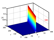
(a)

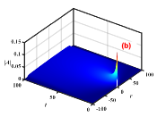
(b)

Figure 1: The spatial-temporal evolution of the one-soliton solution (a) with and (b) without nonlinearity, where $k_{r}=0.1$ is used.

The one-soliton solution can be verified numerically, by taking $A_{S}(t=0)$ as initial condition, and the spatial-temporal evolution of DW is shown in Fig. 1a. It is observed that the initial envelope propagates radially, with its shape and amplitude preserved. On the other hand, in the absence of nonlinearity, the evolution equation of DW can be derived from Eq. (20), which is a linear Schrödinger (complex diffusion) equation

$$\left(\partial_{T}-{\rm i}\tau^{2}\partial_{\xi}^{2}\right)\hat{A} = 0,$$ (22)

which then describes the envelope of DW decays as dispersive wave packet $\hat{A}\propto 1/\sqrt{T}\exp(-\xi^{2}/(\tau^{2}T))$, i.e., the amplitude of DW decreases and its width becomes wider to preserve the “mass” $W$, as shown in Fig. (1b). However, in the presence of nonlinearity, the linear dispersiveness is balanced by nonlinear trapping effect induced by the forced-driven ZF, and thus, soliton solution can be established, as shown in Fig. 1a.

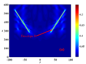
(a)

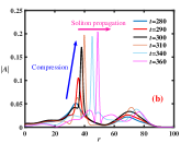
(b)

Figure 2: (a) The spatial-temporal evolution of the initial noise in uniform plasmas, with the red arrow pointing at the envelope “B”. (b) Snapshots of the radial mode structure of DW at a sequence of time, corresponding to the time in Fig. (a).

The forced-driven process may occur when DW amplitude is still small. Thus, it is worthwhile to demonstrate the soliton formation due to ZF self-consistently driven by DW growing from noise level, in the presence of linear growth rate $\gamma_{\rm L}$. In this case, DW is loaded initially as random noise, which grows exponentially due to finite linear growth rate $\gamma_{{\rm L}}$; meanwhile, the growth rate of zonal flow is $2\gamma_{{\rm L}}$. Since there is little saturation mechanism for DW in the present model (no feedback to $\gamma_{\rm L}$ due to ZF scattering), the linear DW growth rate is artificially turned off later to impose saturation. Without loss of generality, $\gamma_{{\rm L}}$ is uniform in space, i.e., $\gamma_{{\rm L}}=\gamma_{{\rm L}0}$ for $t\leq t_{{\rm c}}$, and $\gamma_{{\rm L}}=0$ for $t>t_{{\rm c}}$, where $t_{{\rm c}}$ is the time of “saturation”. The spatial-temporal evolution of DW is shown in Fig. 2a, where $t_{{\rm c}}=300$, $\gamma_{{\rm L0}}=0.025$ and $A_{0}=10^{-4}$ are adopted, with $A_{0}$ being the amplitude of initial noise. It is found that after its amplitude reaches certain threshold at $t\simeq 280$, the soliton structure formation can be observed with a significant compression process, which is more clearly shown in Fig. 2b. In the compression process from $t=280$ to $300$, the width of DW envelope decreases and its amplitude grows significantly faster than the linear growth rate, due to the self-trapping by forced-driven ZF and conservation of DW “mass" $W$. As the nonlinear trapping ($\propto|A|^{2}$) balances the dispersiveness, the steady propagation of solitons can be established, as shown by dashed curves in Fig. 2b. To have a better view on the propagation of solitons, the envelope “B” labeled in Fig. 2a is isolated by multiplying the mode structure at $t=310$ with a super-gaussian $\exp(-(r-r_{B})^{4}/L_{B}^{4})$, where $r_{{\rm B}}$ is the position of the peak of “B”, and $L_{{\rm B}}$ is the width of the filter. The evolution of the envelope “B” is shown in Fig. 3, in which a soliton with periodically oscillating amplitude can be observed. Thus, it is demonstrated that in uniform plasmas, linearly unstable DW with a small initial amplitude can form soliton structures after its amplitude reach certain threshold, with a significant compression.

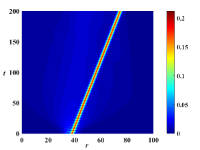
Figure 3: The spatial-temporal evolution of the envelope “B” of Fig. 2a.

The results shown above manifest the important feature of soliton generation due to the forced-driven ZF, but it requires sufficiently large DW amplitude. Thus, it is necessary to find out the threshold for soliton formation to determine the relevance to realistic tokamak plasmas. When dispersiveness dominates over the nonlinearity, DW envelope decays with time as demonstrated by Eq. (22). It is thus expected that as DW amplitude increases, the decay rate of a given envelope should decrease until it reaches steady state, and this defines the threshold on DW amplitude for soliton formation. In Fig. 4, the dependence of decay rate on DW amplitude is given for different DW initial width $L_{{\rm d}}$, with $A_{0}\exp(-r^{2}/L_{{\rm d}}^{2})$ given as initial condition . It is found that even for the case with $L_{\rm d}=10$, the threshold on DW amplitude for steady state soliton formation, is about $e\delta\phi_{n}/T_{\rm i}\simeq 0.02$. Though strictly speaking, soliton structures are characterized by preserving their shape and amplitude during propagation, significant turbulence spreading can be observed when its decay rate is smaller than characteristic time for turbulence spreading, i.e. $L/v_{{\rm g}}$, where $L$ is the system size. As a consequence, the threshold on DW amplitude should be smaller than that corresponding to the vanishing decay rate. The typical DW fluctuation level expected in tokamak experiments is $e\delta\phi_{n}/T_{{\rm i}}\simeq 0.05$, it is, thus, safe to conclude that the threshold on DW amplitude for soliton formation is within the relevant range of experimental and simulation parameters, and may contribute to the turbulence spreading, as shown in Fig. 5, where a DW envelope soliton is given as the initial condition. It is found that the initial DW perturbation flattens very quickly due to the linear dispersiveness in the linear case (L); however, in the nonlinear case (NL), the soliton structure is well preserved, and can, thus, propagate into much broader radial extent than the linear case. Besides, it is also worth mentioning that the threshold for soliton formation decreases with increasing $L_{{\rm d}}$, as shown in Fig. 4,which is consistent with the result given by the inverse scattering method. In fact, dispersiveness becomes weaker for wider (smoother) gaussian envelope, thus, the DW amplitude needed to nonlinearly balance the dispersiveness can be smaller. We note that, strictly speaking, the “turbulence spreading” in uniform plasma should be more precisely understood as propagation of the initial DW perturbation, while the wave packet broadens due to diffusion with $\Delta r\propto\sqrt{t}$, as there is no “linearly stable” or “linearly unstable” regions in uniform plasmas.

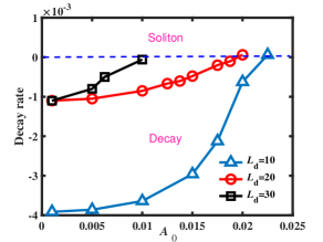
Figure 4: The dependence of decay rate of the envelope on its amplitude, with the triangle, circular and square symbols representing that for the initial width of envelope being 10, 20 and 30. The blue dashed line is the separatrix of decaying envelope and solitons.

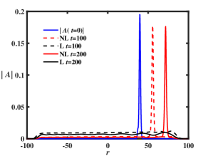
Figure 5: The radial mode structure in both linear and nonlinear cases at $t=100$ and $t=200$, with the envelope “B” of Fig. 2a giving as initial condition. The blue solid curve is the envelope “B”, the black and red dashed lines represent the linear and nonlinear mode structures at $t=100$, respectively, while, the black and red solid lines represent those at $t=200$.

VI DW soliton generation and propagation in nonuniform plasmas

In the last section, it is found that in uniform plasmas the formation of DW solitons can be observed when linear dispersiveness is balanced by nonlinear wave trapping effect induced by the forced-driven ZF, which can contribute to turbulence spreading. However, nonuniformity is intrinsic to magnetically confined plasmas including the excitation of DWs. Consequently, it is particularly important to understand the evolution of DW solitons in nonuniform plasmas. In the present analysis, the plasma nonuniformity is introduced via the radial dependence of the diamagnetic drift frequency, $\varOmega(r)$, in Eq. (16). It is noteworthy that, in Eq. (16), the nonuniformity not only serve as a nonuniform media for wave packet propagation, but also enables the formation of linear DW radial eigenstates before nonlinearity ($\propto|A|^{2}$) becomes significant. For DWs with the amplitude well below the threshold for soliton formation, Eq. (16), in the linear limit, reduces to

$$\left(\partial_{r}^{2}+\dfrac{\omega}{\tau^{2}}+\dfrac{1}{\tau}\varOmega(r)\right)A = 0.$$ (23)

Here, $\omega={\rm i}(\partial_{t}-\gamma_{\rm L})$ is the linear eigenfrequency. For the gaussian-shape nonuniformity considered in this work , i.e., $\varOmega(r)=\exp(-r^{2}/L_{{\rm p}}^{2})-1$, expanding about $r=0$, Eq. (23) becomes approximately the well-known Weber equation. The corresponding eigenfrequency and eigenfunctions are given by

$$A=A_{0}\exp(-r^{2}/(2L_{{\rm d}}^{2})){\rm H}_{\ell}(r/L_{{\rm d}}),$$ (24)

and $\omega=\tau^{3/2}(2n+1)/L_{\rm p}$, respectively, where $L_{{\rm d}}=(\tau L_{{\rm p}}^{2})^{1/4}$, and $H_{\ell}$ is the $\ell$-th Hermite polynomial. Taking the lowest eigenstate as initial condition, Fig. 6a demonstrates that the linearized Eq. (16) does retain the linear eigenmode solution. However, when the amplitude of DW increases and nonlinearity becomes more significant, the linear eigenstates might be qualitatively modified, as shown in Fig. 6b.

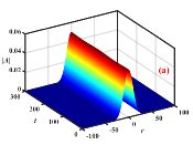
(a)

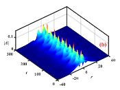
(b)

Figure 6: The spatial-temporal evolution of the lowest eigenstate ($\ell=0$) of the nonuniform plasma (a) without and (b) with nonlinearity. Here, $L_{\rm p}=100$, $A_{0}=0.05$ are used.

Among various potential effects of the nonlinearity on DW envelope evolution, it is particularly important to investigate if and how nonlinearities affect the trajectory of the wavepacket, which could qualitatively determine the radial extent of turbulence spreading. To demonstrate the propagation of solitons, the spatial-temporal evolution of the fourth eigenstate is shown in Fig. 7a, in which propagation and collisions of solitons can be clearly observed. Since trajectories of these solitons overlap with each other, the turning points for each of them is difficult to determine. In order to observe the propagation of a single soliton, soliton “C” labeled in Fig. 7a is, again, isolated by a filter, following the same procedures as that in former section. The spatial-temporal evolution of the soliton “C” is shown in Fig. 7b, where the soliton is reflected back and forth between the turning points located at $\pm r_{\rm tp}$, where the packet velocity vanishes.

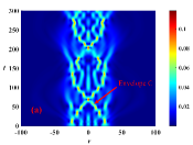
(a)

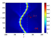
(b)

Figure 7: (a) The spatial-temporal evolution of the fourth order eigenstate, with the red arrow pointing at the envelope “C”. Here, $L_{{\rm p}}=100$ and $A_{0}=0.05$. (b) The spatial-temporal evolution of the envelope “C” alone, whose extent of propagation is bounded inside turning points indicated by two red dashed lines.

By artificially changing the amplitude of the envelope “C”, the dependence of radial position of the turning point $r_{{\rm tp}}$ on DW amplitude (i.e., nonlinearity) can be obtained and shown in Fig. 8. It is found that, within realistically reasonable DW amplitudes, $r_{{\rm tp}}$ is not sensitive to the strength of the nonlinearity, i.e., the radial extent for DW propagation is nearly the same as in the linear case. In the linear limit, the WKB expression is given by Eq. (23), i.e.,

$$\omega+\tau\varOmega(r) = \tau^{2}k_{r}^{2},$$ (25)

and turning points are located at $\tau\varOmega(r_{\rm tp})=\omega$. Assuming a constant $\omega$, we obtain $r_{\rm tp}$ as

$$r_{{\rm tp}} = \pm L_{\rm p}\sqrt{-\ln\left(1-\tau k_{r0}^{2}\right)}.$$ (26)

Here, $k_{r0}=\omega/\tau^{2}$ is the radial wavenumber at $r=0$. It is obvious that $r_{{\rm tp}}$ is proportional to $L_{{\rm p}}$, and increases with increasing $k_{r0}$. The expression for $r_{{\rm tp}}$ given by Eq. (26) can be examined numerically, and the dependence of $r_{{\rm tp}}$ on $k_{r0}$ is shown by the blue solid and dashed curves in Fig. 9a, where theoretical and numerical values agree well with each other.

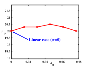
Figure 8: The dependence of $r_{{\rm tp}}$ on the amplitude of soliton “C”, which is adjusted by multiplying the original envelope with ratios.

That the wavepacket propagates, in the lowest order, as in the linear case, suggests taking the envelope as $A=\hat{A}(T,\xi)\exp({\rm i}\int^{r}k_{r}{\rm d}r^{\prime}-{\rm i}\omega t)$, with $k_{r}(r)$ satisfying the linear Eq. (25). The NLSE Eq. (16) then becomes

$$\left[\partial_{T}-{\rm i}\tau^{2}\partial_{\xi}^{2}-{\rm i}\alpha\hat{A}^{2}+\tau^{2}\partial_{r}k_{r}\right.$$

$$\left.-{\rm i}\left(\omega+\tau\varOmega(r)-\tau^{2}k_{r}^{2}\right)\right]\hat{A} = 0,$$ (27)

which, for regions far from the turning points, can be solved perturbatively by expanding $k_{r}$ as $k_{r}=k_{0}+k_{1}+k_{2}+\cdots$, with $k_{0}\gg k_{1}\gg k_{2}\gg\cdots$. Truncating the solution at the first order, the solution is $\hat{A}\propto 1/\sqrt{k_{0}}\exp({\rm i}\int^{r}k_{0}{\rm d}r^{\prime})$, in which $k_{0}=\sqrt{\omega/\tau^{2}+\varOmega(r)/\tau}$, if it is consistently assumed that the amplitude is sufficiently small that it enters at second order in the perturbation expansion. It implies that, as the wavepacket propagates away from local minimum of the potential well, its amplitude can be amplified due to the radial variation of the group velocity, i.e., the fourth term in the left hand side of Eq. (27), and vice versa. While, the trajectory of the envelope, $r_{\rm p}=\int^{t}v_{\rm g}{\rm d}t^{\prime}$, is determined by $k_{0}$, which is not affected by the nonlinearity in the weak amplitude expansion defined above, consistent with Fig. 8.

The WKB solution breaks down near the turning points, in which the potential well can be expanded around the turning points, and Eq. (27) can be reduced to

$$(\partial_{T}-{\rm i}\tau^{2}\partial_{\xi}^{2}-{\rm i}\alpha\hat{A}^{2}-{\rm i}\tau\dfrac{\partial\varOmega}{\partial r}\Delta r)\hat{A} = 0.$$ (28)

Here, $\Delta r=r-r_{\rm p}$ is the small deviation from the turning points. Considering $\partial_{\xi}^{2}\sim 1/\Delta^{2}\sim|\hat{A}|^{2}\gg\Delta r$ ordering for solitons, with $\Delta$ being the width of the wavepacket, Eq. (28) is essentially the NLSE in the moving frame of the wavepacket. This implies that the evolution of the envelope is governed by the same equation as that in uniform plasmas, except for the reflection induced by external potential $\partial\varOmega/\partial r\Delta r$, which can be neglected if the width of the wave packet is smaller than the distance from the turning point. Above all, it is found that the trajectory and turning points of the envelope are determined by the system nonuniformity via $\omega+\tau\varOmega(r)=\tau^{2}k_{r}^{2}$, i.e., Eq. (25). Thus, in nonuniform plasmas, the nonlinearity serves as a local potential well to balance the dispersiveness, while the system nonuniformity serves as a global potential well, which introduces extra trapping effect to the envelope and essentially determines the trajectory for envelope propagation. As a consequence, in nonuniform plasmas, the threshold on DW amplitude for soliton formation could be lower than that in uniform plasmas.

There is another aspect to demonstrate the extra trapping effect of DW by the nonuniformity. The bounce time, which is the period required for the envelope to travel between two turning points $r=-r_{{\rm tp}}$ and $r=r_{{\rm tp}}$, is given by

$$\tau_{{\rm b}} = 2\int_{0}^{r_{{\rm tp}}}\dfrac{{\rm d}r}{v_{{\rm g}}(r)},$$ (29)

where $v_{{\rm g}}(r)=2\tau^{2}\sqrt{k_{r0}^{2}-(1-\exp(-r^{2}/L_{{\rm p}}^{2}))}$ is the group velocity of the envelope. The dependence of $\tau_{{\rm b}}$ on $k_{r0}$ is shown by the red solid curve in Fig. 9a. It is found that for modes with $k_{r0}\leq 0.5$, after being reflected by the turning points, these components with different $k_{r0}$ will meet at $r_{0}$ at almost the same time, though they have different group velocities. The evolution of the envelope “C” in the absence of nonlinearity is shown in Fig. 9b, which can be compared with its nonlinear counterpart in Fig. 7b. It is observed in Fig. 9b that linear dispersiveness dominates the mode dynamics in the beginning, then peaks emerges with time intervals $\varDelta t$ being about 162, which is the $\tau_{{\rm b}}$ corresponding to the envelope “C” with $k_{r0}\leq 0.5$. Thus, the linear potential well introduced by the system nonuniformity has extra trapping effect to the envelopes in the absence of nonliearity, even though the envelope “C” is not a linear radial eigenstate of the system. In fact, it can be observed that the amplitude of peaks decreases each time they emerge, because high-$k_{r}$ modes have larger bounce time, thus, they will not collide at the same time. Here, it is worthwhile drawing a similarity of this phenomenon with the spatial bunching of beam electrons in the beam plasma system O’Neil et al. (1971). Even in that case, in fact, the spatial bunching, which is the counterpart of the amplitude peaking discussed here, is consequence of the “isochronism” in the particle (wave-packet) oscillations. Above all, in nonuniform plasmas, the soliton forms as it is trapped by the localized potential well induced by cubic nonlinearity. Then the soliton is reflected by the global potential well given by system nonuniformity, suppressing the DW turbulence spreading into linearly stable region via soliton generation.

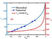
(a)

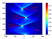
(b)

Figure 9: (a) The dependence of $r_{{\rm tp}}$ and $\tau_{{\rm b}}$ on $k_{r0}$, in which the blue solid curve and blue crosses are the theoretical and numerical values of $r_{\rm tp}$, respectively, corresponding to the vertical axis on the left; while, the red solid curve respresents $\tau_{\rm b}$ given by Eq. (29), corresponding to the vertical axis on the right. (b) The evolution of the envelope “C” alone in the absence of nonlinearity, with the red arrows representing the time and amplitude of the corresponding peaks.

VII Conclusion and discussion

In this work, a paradigm model of drift waves (DWs) self regulation via the forced driven zonal flow (ZF) is derived using nonlinear gyrokinetic theory. The obtained nonlinear DW equation is a nonlinear Schrödinger equation (NLSE), in which the linear dispersiveness, linear growth rate, plasma nonuniformity and cubic nonlinearity induced by feedback of forced driven ZF to DW are self-consistently included. The NLSE is systematically investigated in both uniform and nonuniform plasmas.

In uniform plasmas, soliton structures can form as DW amplitude reaching the threshold for the cubic nonlinearity to balance the linear dispersiveness; and, lead to turbulence spreading via convective DW soliton propagation. The threshold for soliton formation is found to be $e\delta\phi_{n}/T_{{\rm i}}\simeq 0.02$, well within the experimentally relevant parameter regime. As such forced driven generation of ZF by DW turbulence is universally observed in numerical simulations, it is of interest to further investigate the soliton formation in simulations.

In nonuniform plasmas, the evolution of the corresponding linear radial eigenstates is investigated. It is found that the extent for wave propagation is not sensitive to either the existence or strength of the nonlinearity, so in nonuniform plasmas, solitons can not extend beyond the range bounded by the turning points induced by plasma nonuniformity. As a result, in realistic geometry with intrinsic plasma nonuniformity, DW solitons can indeed form, however, it doesn’t further extend turbulence spreading to linearly stable region. The plasma nonuniformity, however, can slightly reduce the threshold on DW amplitude required for soliton generation, due to the additional trapping by the potential well introduced by diamagnetic drift frequency or any other nonuniformity.

An important theoretical progress of this work is the gyrokinetic description of forced-driven excitation of ZF by DWs, commonly observed in numerical simulations, which is a significant component of DW-ZF interactions. It is found that forced-driven excitation of ZF is through the nonlinear ion response to ZF induced by plasma nonuniformity, in contrast to the radial envelope modulation for spontaneous excitation Chen et al. (2000). This mechanism is, in fact, shown to be universal, and has been recently discussed in Ref. Falessi et al. (2023), where the concept of zonal state (ZS) Falessi and Zonca (2019); Zonca et al. (2021) was introduced as the self-consistent plasma equilibrium that is formed due to the excitation of ZF by plasma self-interactions and of their corresponding counterpart in the phase space, i.e., the phase space zonal structures (PSZS) Zonca et al. (2015b). Specific applications are given, e.g., in the ZF forced driven by toroidal Alfvén eigenmode in nonuniform plasmas Chen et al. (2023) to investigate the effects of ZF on Alfvén eigenmode nonlinear saturation and indirect effects on DW stability via forced-driven ZF mediation. Further analyses of these nonlinear interactions leading to self-consistent structure formation and corresponding results will be presented in future publications.

Data availability

The data that support the findings of this study are available from the corresponding author upon reasonable request.

References

- Horton (1999) W. Horton, Rev. Mod. Phys. 71, 735 (1999).
- Lin et al. (1998) Z. Lin, T. S. Hahm, W. W. Lee, W. M. Tang, and R. B. White, Science 281, 1835 (1998).
- Liao et al. (2016) X. Liao, Z. Lin, I. Holod, B. Li, and G. Y. Sun, Physics of Plasmas 23, 122305 (2016).
- Dimits et al. (2000) A. M. Dimits, G. Bateman, M. A. Beer, B. I. Cohen, W. Dorland, G. W. Hammett, C. Kim, J. E. Kinsey, M. Kotschenreuther, A. H. Kritz, et al., Physics of Plasmas 7, 969 (2000).
- Zhao et al. (2006) K. J. Zhao, T. Lan, J. Q. Dong, L. W. Yan, W. Y. Hong, C. X. Yu, A. D. Liu, J. Qian, J. Cheng, D. L. Yu, et al., Phys. Rev. Lett. 96, 255004 (2006).
- Conway et al. (2008) G. D. Conway, C. Troster, B. Scott, K. Hallatschek, and the ASDEX Upgrade Team, Plasma Physics and Controlled Fusion 50, 055009 (2008).
- Lan et al. (2008) T. Lan, A. D. Liu, C. X. Yu, L. W. Yan, W. Y. Hong, K. J. Zhao, J. Q. Dong, J. Qian, J. Cheng, D. L. Yu, et al., Physics of Plasmas 15, 056105 (2008).
- Zhong et al. (2015) W. Zhong, Z. Shi, Y. Xu, X. Zou, X. Duan, W. Chen, M. Jiang, Z. Yang, B. Zhang, P. Shi, et al., Nuclear Fusion 55, 113005 (2015).
- Melnikov et al. (2017) A. Melnikov, L. Eliseev, S. Lysenko, M. Ufimtsev, and V. Zenin, Nuclear Fusion 57, 115001 (2017).
- Chen et al. (2000) L. Chen, Z. Lin, and R. White, Physics of Plasmas 7, 3129 (2000).
- Diamond et al. (2005) P. H. Diamond, S.-I. Itoh, K. Itoh, and T. S. Hahm, Plasma Physics and Controlled Fusion 47, R35 (2005).
- Guzdar et al. (2001) P. N. Guzdar, R. G. Kleva, and L. Chen, Physics of Plasmas 8, 459 (2001).
- Hallatschek and Biskamp (2001) K. Hallatschek and D. Biskamp, Phys. Rev. Lett. 86, 1223 (2001).
- Wang et al. (2020) H. Y. Wang, I. Holod, Z. Lin, J. Bao, J. Y. Fu, P. F. Liu, J. H. Nicolau, D. Spong, and Y. Xiao, Physics of Plasmas 27, 082305 (2020).
- Dong et al. (2019) G. Dong, J. Bao, A. Bhattacharjee, and Z. Lin, Physics of Plasmas 26, 010701 (2019).
- Qiu et al. (2016) Z. Qiu, L. Chen, and F. Zonca, Physics of Plasmas 23, 090702 (2016).
- Todo et al. (2010) Y. Todo, H. Berk, and B. Breizman, Nuclear Fusion 50, 084016 (2010).
- Biancalani et al. (2021) A. Biancalani, A. Bottino, A. D. Siena, O. Gurcan, T. Hayward-Schneider, F. Jenko, P. Lauber, A. Mishchenko, P. Morel, I. Novikau, et al., Plasma Physics and Controlled Fusion 63, 065009 (2021).
- Garbet et al. (1994) X. Garbet, L. Laurent, A. Samain, and J. Chinardet, Nuclear Fusion 34, 963 (1994).
- Hahm et al. (2004) T. S. Hahm, P. H. Diamond, Z. Lin, K. Itoh, and S.-I. Itoh, Plasma Physics and Controlled Fusion 46, A323 (2004).
- Hahm et al. (2005) T. S. Hahm, P. H. Diamond, Z. Lin, G. Rewoldt, O. Gurcan, and S. Ethier, Physics of Plasmas 12, 090903 (2005).
- Zonca et al. (2004) F. Zonca, R. B. White, and L. Chen, Physics of Plasmas 11, 2488 (2004).
- Lin et al. (2002) Z. Lin, S. Ethier, T. S. Hahm, and W. M. Tang, Phys. Rev. Lett. 88, 195004 (2002).
- Guo et al. (2009) Z. Guo, L. Chen, and F. Zonca, Phys. Rev. Lett. 103, 055002 (2009).
- Winsor et al. (1968) N. Winsor, J. L. Johnson, and J. M. Dawson, Physics of Fluids 11, 2448 (1968).
- Zonca and Chen (2008) F. Zonca and L. Chen, Europhys. Lett. 83, 35001 (2008).
- Qiu et al. (2018) Z. Qiu, L. Chen, and F. Zonca, Plasma Science and Technology 20, 094004 (2018).
- Conway et al. (2021) G. D. Conway, A. I. Smolyakov, and T. Ido, Nuclear Fusion (2021).
- Chen et al. (2022) N. Chen, S. Wei, G. Wei, and Z. Qiu, Plasma Physics and Controlled Fusion 64, 015003 (2022).
- Frieman and Chen (1982) E. A. Frieman and L. Chen, Physics of Fluids 25, 502 (1982).
- Rosenbluth and Hinton (1998) M. N. Rosenbluth and F. L. Hinton, Phys. Rev. Lett. 80, 724 (1998).
- Qiu et al. (2014) Z. Qiu, L. Chen, and F. Zonca, Physics of Plasmas 21, 022304 (2014).
- Zonca et al. (2015a) F. Zonca, L. Chen, S. Briguglio, G. Fogaccia, A. V. Milovanov, Z. Qiu, G. Vlad, and X. Wang, Plasma Physics and Controlled Fusion 57, 014024 (2015a).
- O’Neil et al. (1971) T. M. O’Neil, J. H. Winfrey, and J. H. Malmberg, The Physics of Fluids 14, 1204 (1971).
- Falessi et al. (2023) M. V. Falessi, L. Chen, Z. Qiu, and F. Zonca, New Journal of Physics 25, 123035 (2023).
- Falessi and Zonca (2019) M. V. Falessi and F. Zonca, Physics of Plasmas 26, 022305 (2019).
- Zonca et al. (2021) F. Zonca, L. Chen, M. Falessi, and Z. Qiu, Journal of Physics: Conference Series 1785, 012005 (2021).
- Zonca et al. (2015b) F. Zonca, L. Chen, S. Briguglio, G. Fogaccia, G. Vlad, and X. Wang, New Journal of Physics 17, 013052 (2015b).
- Chen et al. (2023) L. Chen, Z. Qiu, F. Zonca, P. Liu, and R. Ma, in Westlake International Symposium on Plasma Physics (Hangzhou, China, 2023).