On max-plus two-sided linear systems whose solution sets are min-plus linear

Abstract

The max-plus algebra $\mathbb{R}\cup\{-\infty\}$ is defined in terms of a combination of the following two operations: addition, $a\oplus b:=\max(a,b)$, and multiplication, $a\otimes b:=a+b$. In this study, we propose a new method to characterize the set of all solutions of a max-plus two-sided linear system $A\otimes\bm{x}=B\otimes\bm{x}$. We demonstrate that the minimum “min-plus” linear subspace containing the “max-plus” solution space can be computed by applying the alternating method algorithm, which is a well-known method to compute single solutions of two-sided systems. Further, we derive a sufficient condition for the “min-plus” and “max-plus” subspaces to be identical. The computational complexity of the method presented in this study is pseudo-polynomial.

Keywords: max-plus algebra, min-plus algebra, tropical semiring, linear system, alternating method, L-convex set

2020MSC: 15A80, 15A06, 15A39

1 Introduction

The max-plus algebra, $\mathbb{R}\cup\{-\infty\}$, is defined in terms of the following two operations: addition, $a\oplus b:=\max(a,b)$, and multiplication, $a\otimes b:=a+b$. The max-plus algebra originated in steelworks [13, 14]. It has a wide range of applications in various fields of science and engineering, such as control theory and scheduling in railway systems [6, 25].

Linear systems over the max-plus algebra have been a popular topic of research for a long time. One-sided systems $A\otimes\bm{x}=\bm{b}$ were solved by the combinatorial way in the 1960s [13]. They were later solved algebraically by introducing a type of dual semiring with two operators: $a\oplus^{\prime}b:=\min(a,b)$ and $a\otimes^{\prime}b:=a+b$ [15]. However, two-sided systems $A\otimes\bm{x}=B\otimes\bm{x}$ are difficult to solve and remain an active topic of research from both theoretical and computational perspectives. A two-sided system can be reduced to a separated system $A\otimes\bm{x}=B\otimes\bm{y}$, which can be solved using the alternating method [17]. Based on the algebraic way to solve one-sided systems, this algorithm alternately applies max-plus and min-plus matrix multiplications. The alternating method is a pseudo-polynomial time algorithm if either $A$ or $B$ is an integer matrix. Currently, there is no known polynomial-time algorithm that can solve general two-sided max-plus linear systems. The existence of a solution to a two-sided system is equivalent to a mean payoff game [1]. Several algorithms have been developed to investigate the general case and its complexities [7, 12, 24]. Tropical linear systems, e.g., $A\otimes\bm{x}$, have also been considered in the literature, in which the solution is a vector such that the maximum $\bigoplus_{j}a_{ij}\otimes x_{j}$ is attained at least twice in each row $i$. This type of solution is obtained based on the theory of tropical geometry over fields with valuation [28, 31]. The solutions of $A\otimes\bm{x}=B\otimes\bm{x}$ are closely related to those of a tropical linear system $(A\oplus B)\otimes\bm{x}$. Further, tropical linear systems can be reduced to max-plus two-sided linear systems. Several algorithms have been proposed to investigate tropical linear systems [18, 19, 23]. In certain cases, either max-plus two-sided systems or tropical linear systems can be solved more efficiently. When the matrix $A$ is of size $n\times(n+1)$, tropical Cramer’s rule can be used to derive a tropical solution in $O(n^{3})$ time [2, 35]. Cramer’s rule has been extended to overdetermined cases [20]. When $A$ and $B$ are square matrices, two-sided max-plus linear systems can be solved under the assumption of idempotency of matrices [8], strong T systems [5], or minimally active or essential systems [27]. Linear systems can also be solved based on the symmetrized max-plus algebra by augmenting “sign-negative” elements and “balanced elements,” which behave as zeros [34]. Then, each term can be moved to the other side of the equality, yielding $(A\ominus B)\otimes\bm{x}=\bm{\varepsilon}$. In particular, this method is useful for solving the system $A\otimes\bm{x}\oplus\bm{c}=B\otimes\bm{x}\oplus\bm{d}$ for square matrices $A$ and $B$ because the inverse of $(A\ominus B)$ can be considered in terms of the symmetrized max-plus algebra. The concept of the symmetrized max-plus algebra has been extended to supertropical algebra and several techniques have been developed to investigate it [26].

The determination of the set of all solutions of max-plus two-sided linear systems is also an important problem. One method to identify all solutions using the usual linear inequalities was presented in [30]. Because the solution set is closed under addition and scalar multiplication in max-plus arithmetic, it is sufficient to determine a generating set of solutions as a max-plus subspace. A fundamental elimination method for deriving a generating set of the solution space was proposed in [10]. Although the elimination step is exhaustive and difficult to execute for large matrices, it ensures that the solution set is a finitely generated max-plus subspace. This idea is applied to derive efficient algorithms with a small number of inequalities [36, 37] and the sparsification method for solving max-plus linear inequalities [29]. Via analogy with polyhedral cone theory, the tropical double description method was proposed to compute a generating set of the solution space [3]. Additionally, tropical Cramer’s rule can be used to solve this problem [33]. The execution of such algorithms requires exponential time in the worst-case scenario. The known upper bound for the cardinality of the basis of the solution space can be expressed in terms of binomial coefficients in the sizes of matrices [4]. The method presented in [21] efficiently finds a large number of solutions based on a given solution.

The purpose of this study is to characterize the solution set of a max-plus two-sided linear system $A\otimes\bm{x}=B\otimes\bm{x}$ from the min-plus linear algebraic perspective. The primary tool used is the alternating method  [17]. As described above, the alternating method computes a single solution for each two-sided system. The obtained solution depends on the initial vectors. Hence, every solution may be obtained via the alternating method if the initial vector is appropriately selected. In the present study, we consider $m$ initial vectors corresponding to the $m$ rows of the system. Then, we obtain $m$ solutions using the alternating method and demonstrate that all the solutions of the system are contained in the min-plus linear subspace generated by these $m$ vectors. In other words, the min-plus closure of the solution set can be computed. In particular, if the solution set is also closed under the “min” operation for vectors, the solution set is then completely determined by applying the alternating method $m$ times. This type of subset plays an important role in combinatorial optimization. A subset that is both max-plus and min-plus linear is called an L-convex set [32]. In this study, we also derive a sufficient condition for the solution set of a two-sided system to be min-plus linear. Although the min-plus linearity of a subset is a global condition, we demonstrate that local min-plus convexity around the $m$ vectors computed using the alternating method is a sufficient condition for it. This implies that the complexity of computing the min-plus linear closure of the solution set as well as that of verifying the min-plus linearity of the solution set are both pseudo-polynomial time for two-sided systems defined by integer matrices.

The remainder of this paper is organized as follows. In Section 2, we introduce basic definitions of max-plus and min-plus linear algebra. In section 3, we summarize the results on max-plus two-sided linear systems and the solutions obtained using the alternating method. Stable solutions with respect to the algorithm play an important role in the discussion. In Section 4, we first restrict the set of solutions to those with finite entries to ensure that the solution set is bounded in the max-plus projective space. Then, we prove that the vectors computed via the alternating method generate the minimum min-plus linear subspace containing all solutions. In Section 5, we present a criterion for the solution set to be min-plus linear. First, we observe that min-plus linearity of a max-plus subspace is characterized in terms of local min-plus convexity. Then, we describe the cell where local min-plus convexity of a solution is violated. Finally, we demonstrate that verification of local min-plus convexity at the vectors computed via the alternating method is sufficient.

2 Max-plus algebra

2.1 Max-plus and min-plus algebras

Let $\mathbb{R}_{\max}=\mathbb{R}\cup\{\varepsilon\}$ be the set of real numbers $\mathbb{R}$ with an extra element $\varepsilon:=-\infty$. We define two operations—addition, $\oplus$, and multiplication, $\otimes$—on $\mathbb{R}_{\max}$ as follows:

$$a\oplus b=\max(a,b),\quad a\otimes b=a+b,\quad a,b\in\mathbb{R}_{\max}.$$

Then, ($\mathbb{R}_{\max},\oplus,\otimes$) is a commutative semiring called the max-plus algebra. Here, $\varepsilon$ is the additive identity and $e:=0$ is the multiplicative identity.

Similarly, the min-plus algebra is denoted by $\mathbb{R}_{\min}=\mathbb{R}\cup\{\varepsilon^{\prime}\}$, where $\varepsilon^{\prime}:=\infty$ and the following two operations hold:

$$a\oplus^{\prime}b=\min(a,b),\quad a\otimes^{\prime}b=a+b,\quad a,b\in\mathbb{R}_{\min}.$$

We extend the operations $\oplus,\otimes,\oplus^{\prime}$, and $\otimes^{\prime}$ to the set $\mathbb{R}_{\max,\min}:=\mathbb{R}\cup\{\varepsilon,\varepsilon^{\prime}\}$ as follows:

$$\varepsilon\oplus\varepsilon^{\prime} =\varepsilon^{\prime}\oplus\varepsilon=\varepsilon^{\prime},\quad\varepsilon\oplus^{\prime}\varepsilon^{\prime}=\varepsilon^{\prime}\oplus^{\prime}\varepsilon=\varepsilon,$$

$$\varepsilon\otimes\varepsilon^{\prime} =\varepsilon^{\prime}\otimes\varepsilon=\varepsilon,\quad\varepsilon\otimes^{\prime}\varepsilon^{\prime}=\varepsilon^{\prime}\otimes^{\prime}\varepsilon=\varepsilon^{\prime}.$$

For further details regarding max-plus and min-plus algebras, please refer to [6, 9, 16, 22, 25, 28, 31].

2.2 Max-plus linear algebra

Let $\mathbb{R}_{\max}^{n}$ and $\mathbb{R}_{\max}^{m\times n}$ be sets of $n$-dimensional max-plus column vectors and $m\times n$ max-plus matrices, respectively. The operations $\oplus$ and $\otimes$, are extended to max-plus vectors and matrices following conventional linear algebra. Let $\bm{\varepsilon}$ and $\mathcal{E}$ denote the max-plus zero vector and the zero matrix, respectively. Further, let $E_{n}$ denote the max-plus unit matrix of order $n$.

A subset of $\mathbb{R}_{\max}^{n}$ is called a max-plus subspace if it is closed under (max-plus) addition and scalar multiplication. For a subset $S\subset\mathbb{R}_{\max}^{n}$, we can easily verify that the set

$$\langle S\rangle_{\max}=\left\{\bigoplus^{r}_{i=1}a_{i}\otimes\bm{x}_{i}\biggm{|}r\in\mathbb{Z}_{>0},\ \bm{x}_{i}\in S,\ a_{i}\in\mathbb{R}_{\max}\text{ for }i=1,2,\dots,r\right\}$$

is a max-plus subspace of $\mathbb{R}_{\max}^{n}$. Subsequently, $\langle S\rangle_{\max}$ is called the max-plus subspace of $\mathbb{R}^{n}_{\max}$ generated by $S$. In particular, the max-plus subspace generated by a finite set $\{\bm{x}_{1},\bm{x}_{2},\dots,\bm{x}_{r}\}$ is denoted by $\langle\bm{x}_{1},\bm{x}_{2},\dots,\bm{x}_{r}\rangle_{\max}$. The minimum generating set of a max-plus subspace is called its basis. In the max-plus algebra, any finitely generated subspace has a basis that is unique up to scalar multiplication [11].

In the present study, we say that the max-plus subspace $V$ is projectively bounded if $V\subset\mathbb{R}^{n}\cup\{\bm{\varepsilon}\}$.

The definitions and notions describe in this subsection extend to analogous ones corresponding to the min-plus algebra. Thus, $\mathbb{R}_{\min}^{n}$ denotes the set of min-plus vectors, $\bm{\varepsilon}^{\prime}$ denotes the min-plus zero vector, etc. A vector or matrix is considered to be finite if it does not contain $\varepsilon$ or $\varepsilon^{\prime}$ as an element.

3 Max-plus linear systems

3.1 Alternating method for solving two-sided systems

The purpose of this study is to investigate all solutions of max-plus homogeneous linear systems

$$A\otimes\bm{x}=B\otimes\bm{x}$$ (3.1)

with $A,B\in\mathbb{R}_{\max}^{m\times n}$. Henceforth, we assume that the coefficient matrices, $A$ and $B$, are doubly $\mathbb{R}$-astic, i.e., all rows and columns contain at least one real number. Let $S(A,B)\subset\mathbb{R}_{\max}^{n}$ be the set of all solutions of (3.1). Then, $S(A,B)$ is a finitely generated max-plus subspace [10]. Although various algorithms have been developed to solve max-plus linear systems, we focus on an iterative algorithm called the alternating method.

First, consider a max-plus linear system with separate variables

$$A\otimes\bm{x}=B\otimes\bm{y},$$ (3.2)

where $A\in\mathbb{R}_{\max}^{m\times n},B\in\mathbb{R}_{\max}^{m\times k}$. Algorithm 3.1 solves the system (3.2). We introduce the following notations. The set $\{1,2,\dots,n\}$ is denoted by $[n]$. In a sequence of vectors $\{\bm{x}(r)\}_{r=0,1,\dots}$, the $i$th entry of $\bm{x}(r)$ is denoted by $x_{i}(r)$. Given $A=(a_{ij})\in\mathbb{R}_{\max}^{m\times n}$, the matrix $-A^{T}=(-a_{ji})\in\mathbb{R}_{\min}^{n\times m}$ is sometimes used as its pseudo-inverse matrix.

Algorithm 3.1 (Alternating Method [17]).

1. Take any vector $\bm{x}(0)\in\mathbb{R}^{n}$ and set $r:=0$.

2. We compute

   $$\bm{y}(r):=-B^{T}\otimes^{\prime}(A\otimes\bm{x}(r)),\quad\bm{x}(r+1):=-A^{T}\otimes^{\prime}(B\otimes\bm{y}(r)).$$

   1. If $x_{i}(r+1)<x_{i}(0)$ for $i\in[n]$, then there is no finite solution of (3.2).

   2. If $\bm{x}(r+1)=\bm{x}(r)$, then $(\bm{x}(r),\bm{y}(r))$ is a solution of (3.2) in $\mathbb{R}^{n}$.

   3. If neither (a) nor (b) holds, then set $r:=r+1$ and repeat (2).

The alternating method is a pseudo-polynomial algorithm. The following results demonstrate the computational complexity of the algorithm.

Proposition 3.2 ([17]).

If $A\in\mathbb{Z}^{m\times n},B\in(\mathbb{Z}\cup\{\varepsilon\})^{m\times k}$ and $\bm{x}(0)\in\mathbb{Z}^{n}$, then the alternating method terminates after finitely many steps. Further, if $|x_{i}(0)|$ is bounded by $K:=\max_{i,j}|a_{ij}|$, the computational complexity is $O(mn(n+k)K)$.

Now, we consider the max-plus linear system (3.1). This system is equivalent to the following system with separate variables:

$$\begin{pmatrix}A\\ B\end{pmatrix}\otimes\bm{x}=\begin{pmatrix}E_{m}\\ E_{m}\end{pmatrix}\otimes\bm{y}.$$ (3.3)

Hence, we can obtain a finite solution of (3.1) by applying the alternating method to (3.3). When $A=(a_{ij}),B=(b_{ij})\in\mathbb{Z}^{m\times n}$, the computational complexity of the alternating method for (3.1) is $O(mn(m+n)K)$, where $K=\max(\max_{i,j}|a_{ij}|,\max_{i,j}|b_{ij}|)$. One iteration step of the Algorithm 3.1 for (3.3) proceeds as follows:

$$\varphi_{0}(\bm{x}):= \begin{pmatrix}-A^{T}&-B^{T}\end{pmatrix}\otimes^{\prime}\left(\begin{pmatrix}E_{m}\\ E_{m}\end{pmatrix}\otimes\left(\begin{pmatrix}-E_{m}^{T}&-E_{m}^{T}\end{pmatrix}\otimes^{\prime}\left(\begin{pmatrix}A\\ B\end{pmatrix}\otimes\bm{x}\right)\right)\right)$$

$$= (-A^{T}\oplus^{\prime}-B^{T})\otimes^{\prime}((A\otimes\bm{x})\oplus^{\prime}(B\otimes\bm{x})).$$

Example 3.3.

Consider the linear system (3.1) for

$$A=\begin{pmatrix}0&1&-1\\ 0&-5&-5\\ 0&4&6\\ 0&3&-2\end{pmatrix},\quad B=\begin{pmatrix}0&-1&-1\\ 0&-4&-3\\ -1&1&6\\ -1&3&-3\end{pmatrix}.$$

Let $\bm{x}(0)=(0,4,3)^{T}$ be the initial vector of the alternating method. Then, we have:

$$\bm{x}(1) =\begin{pmatrix}0&0&0&0\\ -1&4&-4&-3\\ 1&3&-6&2\end{pmatrix}\otimes^{\prime}\left(\begin{pmatrix}5\\ 0\\ 9\\ 7\end{pmatrix}\oplus^{\prime}\begin{pmatrix}3\\ 0\\ 9\\ 7\end{pmatrix}\right)=\begin{pmatrix}0\\ 2\\ 3\end{pmatrix},$$

$$\bm{x}(2) =\begin{pmatrix}0&0&0&0\\ -1&4&-4&-3\\ 1&3&-6&2\end{pmatrix}\otimes^{\prime}\left(\begin{pmatrix}3\\ 0\\ 9\\ 5\end{pmatrix}\oplus^{\prime}\begin{pmatrix}2\\ 0\\ 9\\ 5\end{pmatrix}\right)=\begin{pmatrix}0\\ 1\\ 3\end{pmatrix},$$

$$\bm{x}(3) =\begin{pmatrix}0&0&0&0\\ -1&4&-4&-3\\ 1&3&-6&2\end{pmatrix}\otimes^{\prime}\left(\begin{pmatrix}2\\ 0\\ 9\\ 4\end{pmatrix}\oplus^{\prime}\begin{pmatrix}2\\ 0\\ 9\\ 4\end{pmatrix}\right)=\begin{pmatrix}0\\ 1\\ 3\end{pmatrix}.$$

Hence, $\bm{x}=(0,1,3)^{T}$ is the solution to (3.1).

3.2 Stable solutions obtained via the alternating method

Let us consider the max-plus linear system (3.1). By applying Algorithm 3.1 to the max-plus linear system (3.3), the monotonicity and stability of the iteration are evident. Let $\bm{x}(r)$ denote the vector in $r$th iteration of Algorithm 3.1.

Lemma 3.4 ([17]).

The sequence $\{\bm{x}(r)\}_{r=1,2,\cdots}$ is non-increasing, i.e., $\bm{x}(r+1)\leq\bm{x}(r)$ for $r\geq 1$.

Lemma 3.5 ([17]).

If $\bm{x}$ is a solution of (3.1), then $\varphi_{0}(\varphi_{0}(\bm{x}))=\varphi_{0}(\bm{x})$.

A solution to (3.1) that satisfies $\varphi_{0}(\bm{x})=\bm{x}$ is called a stable solution. The solution obtained via the alternating method is stable. As $\bm{x}\in S(A,B)$ implies $A\otimes\bm{x}=B\otimes\bm{x}$, a stable solution also satisfies

$$\bm{x}=(-A^{T})\otimes^{\prime}(A\otimes\bm{x})\oplus^{\prime}(-B^{T})\otimes^{\prime}(B\otimes\bm{x}).$$ (3.4)

The set of all stable solutions is denoted by $\tilde{S}(A,B)$.

Let $A_{i}$ and $B_{i}$ denote the $i$th rows of $A$ and $B$, respectively. For the system (3.1) and each $i\in[m]$, we define the following set:

$$M^{i}(\bm{x})=\{k\in[n]\ |\ A_{i}\otimes\bm{x}=a_{ik}\otimes x_{k}\ \text{or}\ B_{i}\otimes\bm{x}=b_{ik}\otimes x_{k}\}.$$

Then, stable solutions are characterized by the following proposition:

Proposition 3.6.

If the solution $\bm{x}\in S(A,B)$ satisfies $\bigcup_{i=1}^{m}M^{i}(\bm{x})=[n]$, then $\bm{x}$ is stable.

Proof.

We derive the equality $\bm{x}=(-A^{T})\otimes^{\prime}(A\otimes\bm{x})\oplus^{\prime}(-B^{T})\otimes^{\prime}(B\otimes\bm{x})$. The right-hand side of this equality can be expanded as follows:

$$(-A^{T})\otimes^{\prime}(A\otimes\bm{x})\oplus^{\prime}(-B^{T})\otimes^{\prime}(B\otimes\bm{x})$$

$$= \bigoplus_{i=1}^{m}\!\text{\Large${}^{\prime}$ }\left((-A_{i}^{T})\otimes^{\prime}(A_{i}\otimes\bm{x})\oplus^{\prime}(-B_{i}^{T})\otimes^{\prime}(B_{i}\otimes\bm{x})\right).$$

For $i\in[m]$, let $k\in[n]$ be an index such that $A_{i}\otimes\bm{x}=a_{ik}\otimes x_{k}$ or $B_{i}\otimes\bm{x}=b_{ik}\otimes x_{k}$. Then, we have either

$$[(-A_{i}^{T})\otimes^{\prime}(A_{i}\otimes\bm{x})]_{k}=-a_{ik}\otimes^{\prime}(a_{ik}\otimes x_{k})=x_{k}$$

or

$$[(-B_{i}^{T})\otimes^{\prime}(B_{i}\otimes\bm{x})]_{k}=-b_{ik}\otimes^{\prime}(b_{ik}\otimes x_{k})=x_{k},$$

where $[*]_{k}$ denotes the $k$th entry of the vector. Therefore, we have

$$[(-A_{i}^{T})\otimes^{\prime}(A_{i}\otimes\bm{x})\oplus^{\prime}(-B_{i}^{T})\otimes^{\prime}(B_{i}\otimes\bm{x})]_{k}\leq x_{k}.$$

Hence, the assumption $\bigcup_{i=1}^{m}M^{i}(\bm{x})=[n]$ implies

$$\bigoplus_{i=1}^{m}\!\text{\large${}^{\prime}$ }(-A_{i}^{T})\otimes^{\prime}(A_{i}\otimes\bm{x})\oplus^{\prime}(-B_{i}^{T})\otimes^{\prime}(B_{i}\otimes\bm{x})\leq\bm{x}.$$

However, we can easily verify that any vector $\bm{x}$ satisfies

$$(-A^{T})\otimes^{\prime}(A\otimes\bm{x})\geq\bm{x}$$

and that a similar inequality holds for $B$. Hence, we have

$$\bm{x}\leq(-A^{T})\otimes^{\prime}(A\otimes\bm{x})\oplus^{\prime}(-B^{T})\otimes^{\prime}(B\otimes\bm{x}).$$

This completes the proof of the proposition. ∎

4 Description of solutions as min-plus linear subspaces

For any $A,B\in\mathbb{R}_{\max}^{m\times n}$, a finite solution of the max-plus linear system (3.1) can be determined using the alternating method. However, determining the solution set $S(A,B)$ is a rather difficult problem. We demonstrate that the alternating method can be used to resolve this problem effectively, especially when $S(A,B)$ is also min-plus linear.

4.1 Projectively bounded solution spaces

For $\alpha,\beta\in\mathbb{R}$, consider the following matrix:

$$D_{\alpha,\beta}:=\begin{pmatrix}\alpha&\beta&\cdots&\cdots&\beta\\ \beta&\alpha&&&\vdots\\ \vdots&&\ddots&&\vdots\\ \vdots&&&\alpha&\beta\\ \beta&\cdots&\cdots&\beta&\alpha\end{pmatrix}.$$

Then, the following lemma holds.

Lemma 4.1.

For any $\alpha>0$, we have

$$S(D_{\alpha,0},D_{\alpha,-1})=\{\bm{x}\in\mathbb{R}^{n}\ |\ |x_{j}-x_{k}|\leq\alpha\text{ for }j,k\in[n]\}\cup\{\bm{\varepsilon}\}.$$

Proof.

For any vector $\bm{x}\in\mathbb{R}^{n}$, we have the following equivalence relations:

$$\bm{x}\in S(D_{\alpha,0},D_{\alpha,-1})$$

$$\Longleftrightarrow\quad \alpha\otimes x_{k}\oplus\bigoplus_{i\neq k}x_{i}=\alpha\otimes x_{k}\oplus\bigoplus_{i\neq k}(-1)\otimes x_{i}\quad({}^{\forall}k\in[n])$$

$$\Longleftrightarrow\quad \alpha\otimes x_{k}\geq\bigoplus_{i\neq k}x_{i}\quad({}^{\forall}k\in[n])$$

$$\Longleftrightarrow\quad \alpha\otimes x_{k}\geq x_{j}\quad({}^{\forall}j,k\in[n])$$

$$\Longleftrightarrow\quad \alpha\geq x_{j}-x_{k}\quad({}^{\forall}j,k\in[n])$$

$$\Longleftrightarrow\quad |x_{j}-x_{k}|\leq\alpha\quad({}^{\forall}j,k\in[n]).$$

We can also verify that all solutions except $\bm{\varepsilon}$ are finite. ∎

When we consider the system (3.1), it is helpful to introduce the matrix $C=(c_{ij})=-(A\oplus B)\in\mathbb{R}_{\min}^{m\times n}$.

Proposition 4.2.

For $A,B\in\mathbb{R}_{\max}^{m\times n}$, let $\alpha$ be any real number larger than $\max\{c_{ij}-c_{ik}\mid i\in[m],\ j,k\in[n],\ c_{ij},c_{ik}\in\mathbb{R}\}$. Then, the solution set $S(A,B)$ is projectively bounded if and only if $S(A,B)\subset S(D_{\alpha,0},D_{\alpha,-1})$.

Proof.

“If” part: By Lemma 4.1, $S(D_{\alpha,0},D_{\alpha,-1})$ is projectively bounded. Hence, $S(A,B)$ is projectively bounded if $S(A,B)\subset S(D_{\alpha,0},D_{\alpha,-1})$.

“Only if” part: Suppose $S(A,B)$ is projectively bounded, but $S(A,B)\not\subset S(D_{\alpha,0},D_{\alpha,-1})$. Then, there exists a vector $\bm{x}=(x_{1},x_{2},\dots,x_{n})^{T}\in S(A,B)$ such that $\bm{x}\not\in S(D_{\alpha,0},D_{\alpha,-1})$. By Lemma 4.1, there exist two indices $j,k\in[n]$, such that

$$x_{j}-x_{k}>\alpha.$$

Because $\alpha>\max_{i,j,k}\{c_{ij}-c_{ik}\}$, we have

$$-c_{ij}\otimes x_{j}>-c_{ik}\otimes x_{k}$$

for all $i\in[m]$. Therefore, we have

$$(A_{i}\oplus B_{i})\otimes\bm{x}>(a_{ik}\oplus b_{ik})\otimes x_{k}$$

for all $i\in[m]$. Hence, $(x_{1},x_{2},\dots,x_{k-1},\varepsilon,x_{k+1},\dots,x_{n})^{T}$ is also present in $S(A,B)$. This result contradicts the fact that $S(A,B)$ is projectively bounded. ∎

Let us consider matrices

$$\tilde{A}_{\alpha}=\begin{pmatrix}A\\ D_{\alpha,0}\end{pmatrix},\quad\tilde{B}_{\alpha}=\begin{pmatrix}B\\ D_{\alpha,-1}\end{pmatrix}.$$ (4.1)

From Proposition 4.2, we have $S(A,B)=S(\tilde{A}_{\alpha},\tilde{B}_{\alpha})$ if $S(A,B)$ is projectively bounded. Even when $S(A,B)$ is not projectively bounded, for any $\bm{x}\in S(A,B)\cap\mathbb{R}^{n}$, there exists a real number $\alpha>0$ such that $\bm{x}\in S(\tilde{A}_{\alpha},\tilde{B}_{\alpha})$. Hence, the set $S(\tilde{A}_{\alpha},\tilde{B}_{\alpha})$ can be considered to be an approximation of $S(A,B)$ for large $\alpha$. The system $\tilde{A}_{\alpha}\otimes\bm{x}=\tilde{B}_{\alpha}\otimes\bm{x}$ exhibits good properties when the alternating method is applied to it.

Proposition 4.3.

For any $\alpha>0$, every solution to $\tilde{A}_{\alpha}\otimes\bm{x}=\tilde{B}_{\alpha}\otimes\bm{x}$ is stable.

Proof.

Consider any vector, $\bm{x}\in S(\tilde{A}_{\alpha},\tilde{B}_{\alpha})$. Then, for any $k\in[n]$, the $(m+k)$th equation implies that

$$\alpha\otimes x_{k}\oplus\bigoplus_{i\neq k}x_{i}=\alpha\otimes x_{k}.$$

This implies that $k\in M^{m+k}(\bm{x})$; hence, $\bigcup_{i=1}^{m+n}M^{i}(\bm{x})=[n]$. Proposition 3.6 implies that $\bm{x}$ is a stable solution of $\tilde{A}_{\alpha}\otimes\bm{x}=\tilde{B}_{\alpha}\otimes\bm{x}$. ∎

4.2 Min-plus linear closure of the solution set

In this section, we characterize the max-plus subspace $S(A,B)$ from a min-plus algebraic perspective. Based on Proposition 4.3, we consider the system $\tilde{A}_{\alpha}\otimes\bm{x}=\tilde{B}_{\alpha}\otimes\bm{x}$ instead of the system (3.1), and assume that all solutions are stable, i.e., $S(A,B)=\tilde{S}(A,B)$. Further, we assume that $S(A,B)$ is projectively bounded. Let $\varphi(\bm{x})$ be the solution of (3.1) obtained by applying the alternating method to $\bm{x}(0):=\bm{x}$. We use the notation $C=-(A\oplus B)\in\mathbb{R}_{\min}^{m\times n}$. The $i$th row of $C$ is denoted by $C_{i}$.

Proposition 4.4.

For any matrix $A,B\in\mathbb{R}_{\max}^{m\times n}$, we have

$$S(A,B)\subset\langle\varphi(C^{T}_{1}),\varphi(C^{T}_{2}),\dots,\varphi(C^{T}_{m})\rangle_{\min}\cup\{\bm{\varepsilon}\}.$$

Proof.

Consider any vector $\bm{x}\in S(A,B)\setminus\{\bm{\varepsilon}\}$. Because $\bm{x}$ is a stable solution, the equality (3.4) implies

$$\bm{x}=\bigoplus_{i=1}^{m}\!\text{\large${}^{\prime}$ }t_{i}\otimes^{\prime}C^{T}_{i},$$

where $t_{i}$ denotes the $i$th entry of $A\otimes\bm{x}$ (or, equivalently, the $i$th entry of $B\otimes\bm{x}$). Based on the monotonicity of the operator $\varphi$, we have $\bm{x}=\varphi(\bm{x})\leq\varphi(t_{i}\otimes^{\prime}C_{i}^{T})$. Hence, we have

$$\bm{x}\leq\bigoplus_{i=1}^{m}\!\text{\large${}^{\prime}$ }\varphi(t_{i}\otimes^{\prime}C^{T}_{i})=\bigoplus_{i=1}^{m}\!\text{\large${}^{\prime}$ }t_{i}\otimes^{\prime}\varphi(C^{T}_{i}).$$

To demonstrate that $\varphi(C_{i}^{T})\leq C_{i}^{T}$, it is sufficient to derive $\varphi_{0}(C_{i}^{T})\leq C_{i}^{T}$ because $\varphi(C_{i}^{T})\leq\varphi_{0}(C_{i}^{T})$ holds by Lemma 3.4. We first note that $(A_{i}\otimes C_{i}^{T})\oplus^{\prime}(B_{i}\otimes C^{T}_{i})=0$ as $C_{i}=-(A_{i}\oplus B_{i})$. Then, we have

$$\varphi_{0}(C_{i}^{T}) =C^{T}\otimes^{\prime}((A\otimes C_{i}^{T})\oplus^{\prime}(B\otimes C^{T}_{i}))$$

$$=\bigoplus_{k=1}^{m}\!\text{\large${}^{\prime}$ }((A_{k}\otimes C_{i}^{T})\oplus^{\prime}(B_{k}\otimes C^{T}_{i}))\otimes^{\prime}C_{k}^{T}$$

$$=C_{i}^{T}\oplus^{\prime}\bigoplus_{k\neq i}\!\text{\large${}^{\prime}$ }((A_{k}\otimes C_{i}^{T})\oplus^{\prime}(B_{k}\otimes C^{T}_{i}))\otimes^{\prime}C_{k}^{T}$$

$$\leq C_{i}^{T}.$$

Thus, we have $\varphi(C_{i}^{T})\leq C_{i}^{T}$; hence,

$$\bigoplus_{i=1}^{m}\!\text{\large${}^{\prime}$ }t_{i}\otimes^{\prime}\varphi(C^{T}_{i})\leq\bigoplus_{i=1}^{m}\!\text{\large${}^{\prime}$ }t_{i}\otimes^{\prime}C^{T}_{i}=\bm{x}.$$

This proves the equality

$$\bm{x}=\bigoplus_{i=1}^{m}\!\text{\large${}^{\prime}$ }t_{i}\otimes^{\prime}\varphi(C^{T}_{i}),$$

which implies that $\bm{x}\in\langle\varphi(C^{T}_{1}),\varphi(C^{T}_{2}),\dots,\varphi(C^{T}_{m})\rangle_{\min}$. Hence, we conclude that $S(A,B)\subset\langle\varphi(C^{T}_{1}),\varphi(C^{T}_{2}),\dots,\varphi(C^{T}_{m})\rangle_{\min}\cup\{\bm{\varepsilon}\}$, ∎

For a projectively bounded max-plus subspace $V\subset\mathbb{R}_{\max}^{n}$, the smallest min-plus subspace of $\mathbb{R}_{\min}^{n}$ containing $V\setminus\{\bm{\varepsilon}\}$ is defined to be the min-plus linear closure of $V$. A projectively bounded max-plus subspace $V\subset\mathbb{R}_{\max}^{n}$ is called min-plus linear if $(V\setminus\{\bm{\varepsilon}\})\cup\{\bm{\varepsilon}^{\prime}\}$ is a min-plus subspace of $\mathbb{R}_{\min}^{n}$. The following corollary asserts that the min-plus linear closure of the solution set $S(A,B)$ can be obtained via the alternating method.

Corollary 4.5.

For any matrix $A,B\in\mathbb{R}_{\max}^{m\times n}$, the min-plus linear closure of $S(A,B)\setminus\{\bm{\varepsilon}\}$ is

$$\langle\varphi(C^{T}_{1}),\varphi(C^{T}_{2}),\ldots,\varphi(C^{T}_{m})\rangle_{\min}.$$

In particular, if $S(A,B)$ is min-plus linear, then

$$S(A,B)\setminus\{\bm{\varepsilon}\}=\langle\varphi(C^{T}_{1}),\varphi(C^{T}_{2}),\ldots,\varphi(C^{T}_{m})\rangle_{\min}\setminus\{\bm{\varepsilon}^{\prime}\}.$$

Example 4.6.

We consider the following matrices

$$A=\begin{pmatrix}0&1&-1\\ 0&-5&-5\\ 0&4&6\\ 0&3&-2\\ \alpha&0&0\\ 0&\alpha&0\\ 0&0&\alpha\end{pmatrix},\quad B=\begin{pmatrix}0&-1&-1\\ 0&-4&-3\\ -1&1&6\\ -1&3&-3\\ \alpha&-1&-1\\ -1&\alpha&-1\\ -1&-1&\alpha\end{pmatrix},$$

obtained from the matrices in Example 3.3 via extension (4.1). We set $\alpha=13$. Then, by setting

$$C_{1}=(0,-1,1), \quad C_{2}=(0,4,3),\quad C_{3}=(0,-4,-6),\quad C_{4}=(0,-3,2),$$

$$C_{5} =(\alpha,0,0),\quad C_{6}=(0,\alpha,0),\quad C_{7}=(0,0,\alpha),$$

we have

$$\varphi(C_{1})=(0,-1,1)^{T},\quad\varphi(C_{2})=(0,1,3)^{T},$$

$$\varphi(C_{3})\sim(0,-3,-5)^{T},\quad\varphi(C_{4})=(0,-3,2)^{T},$$

$$\varphi(C_{5})\sim( 0,-3,-5)^{T},\quad\varphi(C_{6})\sim(0,-1,0)^{T},\quad\varphi(C_{7})\sim(0,-1,3)^{T},$$

where scalar multiples are modified for $C_{3},C_{5},C_{6}$, and $C_{7}$ so that the first entries are $0$. The min-plus subspace generated by these seven vectors is illustrated by the shaded region in Figure 1.

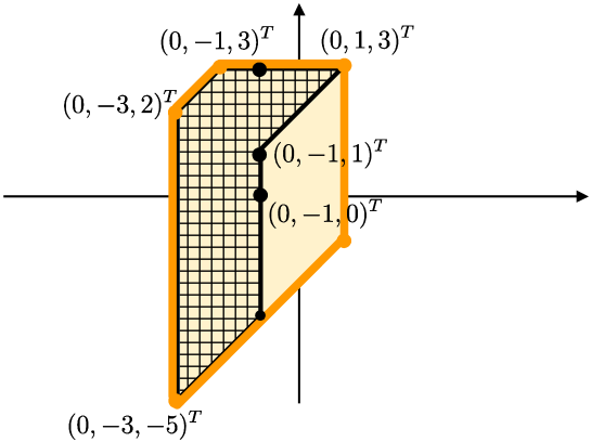
Figure 1: The solution set, $S(A,B)$, projected onto $x_{1}=0$ (lattice pattern) and its min-plus linear closure (shaded).

5 A criterion for the solution set to be min-plus linear

By Corollary 4.5, the solution set $S(A,B)$ can be computed via the alternating method if it is min-plus linear. In this section, we present a sufficient condition for the solution set $S(A,B)$ to be min-plus linear. First, we introduce the concept of local min-plus convex sets. We define the distance between $\bm{x}=(x_{1},x_{2},\dots,x_{n})^{T}\in\mathbb{R}^{n}$ and $\bm{y}=(y_{1},y_{2},\dots,y_{n})^{T}\in\mathbb{R}^{n}$ as follows:

$$d(\bm{x},\bm{y})=\max_{i\in[n]}|x_{i}-y_{i}|.$$

The $r$-neighborhood of $\bm{x}=(x_{1},x_{2},\dots,x_{n})^{T}\in\mathbb{R}^{n}$ is defined as

$$\mathcal{N}(\bm{x},r)=\{\bm{y}\in\mathbb{R}^{n}\ |\ d(\bm{x},\bm{y})<r\}$$

for $r>0$.

Definition 5.1.

Let $S\subset\mathbb{R}^{n}\cup\{\bm{\varepsilon}\}$ be a subset closed under scalar multiplication. Then, $S$ is said to be locally min-plus convex at $\bm{x}\in S\setminus\{\bm{\varepsilon}\}$ if there exists $r>0$ such that $\bm{y}\oplus^{\prime}\bm{z}\in S$ holds for any $\bm{y},\bm{z}\in\mathcal{N}(\bm{x},r)\cap S$.

In fact, the min-plus local convexity at every point of the max-plus subspace is equivalent to global min-plus linearity.

Proposition 5.2.

Let $S\subset\mathbb{R}_{\max}^{n}$ be a projectively bounded max-plus subspace. Then, $S$ is min-plus linear if and only if it is locally min-plus convex for any $\bm{x}\in S\setminus\{\bm{\varepsilon}\}$.

Proof.

The “only if” part is trivial. We need to prove the “if” part of the proposition. Suppose that $S$ is not min-plus linear. Then, there exist two vectors $\bm{x},\bm{y}\in S\setminus\{\bm{\varepsilon}\}$ such that $\bm{x}\oplus^{\prime}\bm{y}\not\in S$. We will find the point $\bm{p}^{*}\in S$ where $S$ is not locally min-plus convex, as shown in Figure 2. Consider the minimum positive number $\alpha$ such that

$$\bm{z}:=\alpha\otimes^{\prime}\bm{x}\oplus^{\prime}\bm{y}\in S.$$

By minimality of $\alpha$, we have

$$\bm{z}(\delta):=(\alpha-\delta)\otimes^{\prime}\bm{x}\oplus^{\prime}\bm{y}\not\in S$$

when $0<\delta<\alpha$. Further, let $\beta(\delta)$ be the maximum number such that

$$\bm{x}\oplus\beta(\delta)\otimes\bm{z}(\delta)\in S.$$

We set $\bm{u}(\delta)=\delta\otimes(\bm{x}\oplus\beta(\delta)\otimes\bm{z}(\delta))$. By maximality of $\beta(\delta)$, we have

$$\bm{v}(\delta):=\bm{x}\oplus(\beta(\delta)+\delta)\otimes\bm{z}(\delta)\not\in S.$$

As $S$ is a max-plus subspace, we have

$$\bm{w}(\delta):=\bm{x}\oplus(\beta(\delta)+\delta)\otimes\bm{z}\in S.$$

Now, we prove that $\bm{u}(\delta),\bm{v}(\delta)$ and $\bm{w}(\delta)$ are contained in the neighborhood of a certain fixed point $\bm{p}^{*}$ and satisfy $\bm{v}(\delta)=\bm{u}(\delta)\oplus^{\prime}\bm{w}(\delta)$. First, we determine $\bm{p}^{*}$ by demonstrating that $\lim_{\delta\to+0}\beta(\delta)$ exists.

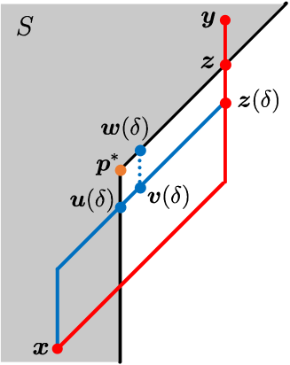
Figure 2: Proof of Lemma 5.2.

Lemma 5.3.

If $0<\delta^{\prime}<\delta$, then $\beta(\delta)\leq\beta(\delta^{\prime})$. Further, when $0<\delta<1$, $\beta(\delta)$ is bounded above.

Proof.

Let $\bm{x}=(x_{1},x_{2},\dots,x_{n})^{T}$ and $\bm{z}=(z_{1},z_{2},\dots,z_{n})^{T}$. Firstly, there exist $\delta>0$ and $I\subset[n]$ such that

$$z_{i}(\delta^{\prime})=\begin{cases}z_{i}&i\in I,\\ z_{i}-\delta^{\prime}&i\not\in I,\end{cases}$$

for any $0<\delta^{\prime}\leq\delta$. Then, we have

$$\bm{z}(\delta^{\prime})=\bm{z}(\delta)\oplus(-\delta^{\prime})\otimes\bm{z}.$$

Because $\bm{x}\oplus\beta(\delta)\otimes\bm{z}(\delta)\in S$, we have

$$\bm{x}\oplus\beta(\delta)\otimes\bm{z}(\delta^{\prime})=(\bm{x}\oplus\beta(\delta)\otimes\bm{z}(\delta))\oplus(\beta(\delta)-\delta^{\prime})\otimes\bm{z}\in S.$$

By maximality of $\beta(\delta^{\prime})$, we have $\beta(\delta)\leq\beta(\delta^{\prime})$. Next, let $\xi=\max_{i}x_{i}$ and $\zeta=\min_{i}z_{i}$. Because $\bm{z}(\delta)\geq(-1)\otimes\bm{z}$ for $\delta<1$, we have:

$$(\xi-\zeta+1)\otimes\bm{z}(\delta)\geq\xi\otimes(0,0,\dots,0)^{T}\geq\bm{x}.$$

Hence, for any $\beta\geq\xi-\zeta+1$, we have:

$$\bm{x}\oplus\beta\otimes\bm{z}(\delta)=\beta\otimes\bm{z}(\delta)\not\in S,$$

which implies that $\beta(\delta)<\xi-\zeta+1$, ∎

Proof of Proposition 5.2 (continued).

By Lemma 5.3, let $\beta^{*}=\lim_{\delta\to+0}\beta(\delta)$. Then, the desired point $\bm{p}^{*}$ is given by

$$\bm{p}^{*}=\bm{x}\oplus\beta^{*}\otimes\bm{z}.$$

Indeed, for any $r>0$, we can verify that $\bm{u}(\delta),\bm{v}(\delta),\bm{w}(\delta)\in\mathcal{N}(\bm{p}^{*},r)$ by taking sufficiently small $\delta>0$ such that $\beta^{*}-\beta(\delta)<\frac{r}{2}$ and $\delta<\frac{r}{2}$.

Next, we demonstrate that $\bm{v}(\delta)=\bm{u}(\delta)\oplus^{\prime}\bm{w}(\delta)$. Because $\bm{z}(\delta)\leq(\alpha-\delta)\otimes^{\prime}\bm{x}$, we have

$$\bm{x}\oplus(\delta-\alpha)\otimes\bm{z}(\delta)=\bm{x}\in S.$$

By maximality of $\beta(\delta)$, we have $\alpha+\beta(\delta)\geq\delta$. We also note that

$$\bm{z}(\delta)=(\alpha-\delta)\otimes^{\prime}\bm{x}\oplus^{\prime}\bm{y}=(\alpha-\delta)\otimes^{\prime}\bm{x}\oplus^{\prime}\alpha\otimes^{\prime}\bm{x}\oplus^{\prime}\bm{y}=(\alpha-\delta)\otimes^{\prime}\bm{x}\oplus^{\prime}\bm{z}.$$

Then, we have

$$\bm{u}(\delta) =\delta\otimes\bm{x}\oplus(\beta(\delta)+\delta)\otimes((\alpha-\delta)\otimes^{\prime}\bm{x}\oplus^{\prime}\bm{z})$$

$$=(\delta\otimes\bm{x}\oplus(\alpha+\beta(\delta))\otimes\bm{x})\oplus^{\prime}(\delta\otimes\bm{x}\oplus(\beta(\delta)+\delta)\otimes\bm{z})$$

$$=((\alpha+\beta(\delta))\otimes\bm{x})\oplus^{\prime}(\delta\otimes\bm{x}\oplus(\beta(\delta)+\delta)\otimes\bm{z}).$$

Here, we use the property $\bm{a}\oplus(\bm{b}\oplus^{\prime}\bm{c})=(\bm{a}\oplus\bm{b})\oplus^{\prime}(\bm{a}\oplus\bm{c})$. Thus, we have

$$\bm{u}(\delta)\oplus^{\prime}\bm{w}(\delta)$$

$$=\, ((\alpha+\beta(\delta))\otimes\bm{x})\oplus^{\prime}(\delta\otimes\bm{x}\oplus(\beta(\delta)+\delta)\otimes\bm{z})\oplus^{\prime}(\bm{x}\oplus(\beta(\delta)+\delta)\otimes\bm{z})$$

$$=\, ((\alpha+\beta(\delta))\otimes\bm{x})\oplus^{\prime}(\bm{x}\oplus(\beta(\delta)+\delta)\otimes\bm{z}).$$

On the other hand, we can express $\bm{v}(\delta)$ as follows

$$\bm{v}(\delta) =\bm{x}\oplus(\beta(\delta)+\delta)\otimes((\alpha-\delta)\otimes^{\prime}\bm{x}\oplus^{\prime}\bm{z})$$

$$=(\bm{x}\oplus(\alpha+\beta(\delta))\otimes\bm{x})\oplus^{\prime}(\bm{x}\oplus(\beta(\delta)+\delta)\otimes\bm{z})$$

$$=((\alpha+\beta(\delta))\otimes\bm{x})\oplus^{\prime}(\bm{x}\oplus(\beta(\delta)+\delta)\otimes\bm{z}),$$

This proves that $\bm{v}(\delta)=\bm{u}(\delta)\oplus^{\prime}\bm{w}(\delta)$. Hence, we conclude that $S(A,B)$ is not min-plus convex at $\bm{p}^{*}\in S$. ∎

Next, we discuss the local min-plus convexity of the solution set $S(A,B)$.

Definition 5.4.

Let $\bm{a}=(a_{1},a_{2},\dots,a_{n}),\bm{b}=(b_{1},b_{2},\dots,b_{n})\in\mathbb{R}^{1\times n}_{\max}$. We define the subset $R(\bm{a},\bm{b})\subset\mathbb{R}^{n}$ consisting of solutions $\bm{x}=(x_{1},x_{2},\dots,x_{n})^{T}$ of a single equation $\bm{a}\otimes\bm{x}=\bm{b}\otimes\bm{x}$ satisfying one of the following conditions:

1. There exist $i,j\in[n],\ i\neq j,$ such that

   $$\bm{a}\otimes\bm{x} =a_{i}\otimes x_{i}>a_{k}\otimes x_{k}\quad\text{ for }k\neq i,\text{ and}$$

   $$\bm{b}\otimes\bm{x} =b_{j}\otimes x_{j}>b_{k}\otimes x_{k}\quad\text{ for }k\neq j.$$

2. There exists $i\in[n]$ such that

   $$\bm{a}\otimes\bm{x} =a_{i}\otimes x_{i},$$

   $$\bm{b}\otimes\bm{x} =b_{i}\otimes x_{i}>b_{k}\otimes x_{k}\quad\text{ for }k\neq i.$$

3. For any $i\in[n]$,

   $$\bm{a}\otimes\bm{x}=a_{i}\otimes x_{i}\quad\Longleftrightarrow\quad\bm{b}\otimes\bm{x}=b_{i}\otimes x_{i}$$

   holds.

Proposition 5.5.

Let $\bm{a}=(a_{1},a_{2},\dots,a_{n}),\bm{b}=(b_{1},b_{2},\dots,b_{n})\in\mathbb{R}^{1\times n}_{\max}\setminus\{\bm{\varepsilon}\}$. For any vector $\bm{x}=(x_{1},x_{2},\dots,x_{n})^{T}\in S(\bm{a},\bm{b})\cap\mathbb{R}^{n}$, (i) and (ii) are equivalent:

1. $S(\bm{a},\bm{b})$ is locally min-plus convex at $\bm{x}$.

2. $\bm{x}\in R(\bm{a},\bm{b})$.

Proof.

(ii) $\Longrightarrow$ (i): Take any vector $\bm{x}\in R(\bm{a},\bm{b})$ and define

$$K(\bm{a},\bm{x}) =\{i\in[n]\mid\bm{a}\otimes\bm{x}=a_{i}\otimes x_{i}\},$$

$$K(\bm{b},\bm{x}) =\{i\in[n]\mid\bm{b}\otimes\bm{x}=b_{i}\otimes x_{i}\}.$$

Then, for sufficiently small $r>0$ and $\bm{y},\bm{z}\in\mathcal{N}(\bm{x},r)\cap S(\bm{a},\bm{b})$, we have

$$a_{i}\otimes y_{i}>a_{k}\otimes y_{k},\quad a_{i}\otimes z_{i}>a_{k}\otimes z_{k}$$

for $i\in K(\bm{a},\bm{x}),k\notin K(\bm{a},\bm{x})$, and

$$b_{i}\otimes y_{i}>b_{k}\otimes y_{k},\quad b_{i}\otimes z_{i} >a_{k}\otimes z_{k}$$

for $i\in K(\bm{b},\bm{x}),k\notin K(\bm{b},\bm{x})$. This yields

$$K(\bm{a},\bm{x})\supset K(\bm{a},\bm{y}),K(\bm{a},\bm{z}),\quad K(\bm{b},\bm{x})\supset K(\bm{b},\bm{y}),K(\bm{b},\bm{z}).$$

• Suppose $\bm{x}$ satisfies condition 1 of Definition 5.4 for $K(\bm{a},\bm{x})=\{i\}$ and $K(\bm{b},\bm{x})=\{j\}$. Then, we have

  $$a_{i}\otimes(y_{i}\oplus^{\prime}z_{i}) >a_{k}\otimes(y_{k}\oplus^{\prime}z_{k})\quad\text{ for }k\neq i,$$

  $$b_{j}\otimes(y_{j}\oplus^{\prime}z_{j}) >a_{k}\otimes(y_{k}\oplus^{\prime}z_{k})\quad\text{ for }k\neq j.$$

  Therefore, we compute

  $$\bm{a}\otimes(\bm{y}\oplus^{\prime}\bm{z}) =a_{i}\otimes(y_{i}\oplus^{\prime}z_{i})$$

  $$=(a_{i}\otimes y_{i})\oplus^{\prime}(a_{i}\otimes z_{i})$$

  $$=(b_{j}\otimes y_{j})\oplus^{\prime}(b_{j}\otimes z_{j})$$

  $$=b_{j}\otimes(y_{j}\oplus^{\prime}z_{j})$$

  $$=\bm{b}\otimes(\bm{y}\oplus^{\prime}\bm{z})$$

  This proves that $\bm{y}\oplus^{\prime}\bm{z}\in S(\bm{a},\bm{b})$.

• Suppose $\bm{x}$ satisfies condition 2 of Definition 5.4 for $K(\bm{b},\bm{x})=\{i\}$, which yields $a_{i}=b_{i}$. Then, we have

  $$a_{i}\otimes y_{i}=b_{i}\otimes y_{i} >b_{k}\otimes y_{k}\quad\text{ for }k\neq i,$$

  $$a_{i}\otimes z_{i}=b_{i}\otimes z_{i} >b_{k}\otimes z_{k}\quad\text{ for }k\neq i,$$

  and hence

  $$a_{i}\otimes y_{i} \geq a_{k}\otimes y_{k}\quad\text{ for }k\neq i,$$

  $$a_{i}\otimes z_{i} \geq a_{k}\otimes z_{k}\quad\text{ for }k\neq i.$$

  Therefore, we have

  $$\bm{a}\otimes(\bm{y}\oplus^{\prime}\bm{z})=a_{i}\otimes(y_{i}\oplus^{\prime}z_{i})=b_{i}\otimes(y_{i}\oplus^{\prime}z_{i})=\bm{b}\otimes(\bm{y}\oplus^{\prime}\bm{z}).$$

  Thus, we see that $\bm{y}\oplus^{\prime}\bm{z}\in S(\bm{a},\bm{b})$.

• Suppose $\bm{x}$ satisfies condition 3 of Definition 5.4. Then, we have

  $$K(\bm{a},\bm{y})=K(\bm{b},\bm{y}),\quad K(\bm{a},\bm{z})=K(\bm{b},\bm{z})$$

  since $a_{i}=b_{i}$ for all $i\in K(\bm{a},\bm{x})=K(\bm{b},\bm{x})$. Therefore, we have

  $$\bm{a}\otimes(\bm{y}\oplus^{\prime}\bm{z}) =a_{i}\otimes(y_{i}\oplus^{\prime}z_{i})$$

  $$=(a_{i}\otimes y_{i})\oplus^{\prime}(a_{i}\otimes z_{i})$$

  $$=(b_{i}\otimes y_{i})\oplus^{\prime}(b_{i}\otimes z_{i})$$

  $$=b_{i}\otimes(y_{i}\oplus^{\prime}z_{i})$$

  $$=\bm{b}\otimes(\bm{y}\oplus^{\prime}\bm{z}).$$

  Thus, we see that $\bm{y}\oplus^{\prime}\bm{z}\in S(\bm{a},\bm{b})$.

Based on these three cases, we conclude that $S(\bm{a},\bm{b})$ is locally min-plus convex at $\bm{x}$.

(i) $\Longrightarrow$ (ii): Consider any vector $\bm{x}\in\mathbb{R}^{n}$ such that $\bm{x}\not\in R(\bm{a},\bm{b})$. Then, we have the following four cases:

1. When $|K(\bm{a},\bm{x})|=|K(\bm{b},\bm{x})|=1$, $K(\bm{a},\bm{x})=K(\bm{b},\bm{x})$ implies condition 3 of Definition 5.4 and $K(\bm{a},\bm{x})\neq K(\bm{b},\bm{x})$ implies condition 1 of Definition 5.4. Hence, this case cannot occur if $\bm{x}\not\in R(\bm{a},\bm{b})$.

2. When $|K(\bm{a},\bm{x})|=1$ and $|K(\bm{b},\bm{x})|\neq 1$, $K(\bm{a},\bm{x})\subset K(\bm{b},\bm{x})$ implies condition 2 in Definition 5.4. Hence, we have $K(\bm{a},\bm{x})\not\subset K(\bm{b},\bm{x})$.

3. When $|K(\bm{a},\bm{x})|\neq 1$ and $|K(\bm{b},\bm{x})|=1$, $K(\bm{b},\bm{x})\not\subset K(\bm{a},\bm{x})$ as in case (b).

4. When $|K(\bm{a},\bm{x})|\neq 1$ and $|K(\bm{b},\bm{x})|\neq 1$, $K(\bm{a},\bm{x})=K(\bm{b},\bm{x})$ implies condition 3 of Definition 5.4. Hence, we have $K(\bm{a},\bm{x})\neq K(\bm{b},\bm{x})$.

From the aforementioned observations, there exist three distinct indices, $i_{1},i_{2},j$, such that:

$$\left\{\begin{array}[]{l}j\in K(\bm{b},\bm{x})\setminus K(\bm{a},\bm{x}),\\ i_{1},i_{2}\in K(\bm{a},\bm{x}),\end{array}\right.$$

or

$$\left\{\begin{array}[]{l}j\in K(\bm{a},\bm{x})\setminus K(\bm{b},\bm{x}),\\ i_{1},i_{2}\in K(\bm{b},\bm{x}).\end{array}\right.$$

In the former case, defining the two vectors $\bm{y}_{1},\bm{y}_{2}$ as

$$\bm{y}_{1}=(x_{1},x_{2},\dots,x_{i_{1}-1},x_{i_{1}}+r,x_{i_{1}+1},\dots,x_{j-1},x_{j}+r,x_{j+1},\dots,x_{n})^{T},$$

$$\bm{y}_{2}=(x_{1},x_{2},\dots,x_{i_{2}-1},x_{i_{2}}+r,x_{i_{2}+1},\dots,x_{j-1},x_{j}+r,x_{j+1},\dots,x_{n})^{T},$$

for a sufficiently small $r>0$, we have

$$\bm{a}\otimes\bm{y}_{1} =\bm{a}\otimes\bm{x}+r=\bm{b}\otimes\bm{x}+r=\bm{b}\otimes\bm{y}_{1},$$

$$\bm{a}\otimes\bm{y}_{2} =\bm{a}\otimes\bm{x}+r=\bm{b}\otimes\bm{x}+r=\bm{b}\otimes\bm{y}_{2}.$$

Hence, $\bm{y}_{1},\bm{y}_{2}\in R(\bm{x},r)\cap S(\bm{a},\bm{b})$. However, the vector $\bm{z}=\bm{y}_{1}\oplus^{\prime}\bm{y}_{2}$ satisfies $\bm{a}\otimes\bm{z}=\bm{a}\otimes\bm{x}$ and $\bm{b}\otimes\bm{z}=\bm{b}\otimes\bm{x}+r$, which yields $\bm{a}\otimes\bm{z}\neq\bm{b}\otimes\bm{z}$. Because $r>0$ can be taken to be arbitrarily small, $S(A,B)$ cannot be locally min-plus convex at $\bm{x}$. ∎

To verify the min-plus linearity of the solution set $S(A,B)$, the local min-plus convexity at only some special points needs to be verified. First, we present the following technical lemma.

Lemma 5.6.

If $\bm{y}\in S(A,B)$ satisfies $\bm{y}\leq\bm{x}$ for $\bm{x}\in\mathbb{R}^{n}$, then $\bm{y}\leq\varphi(\bm{x})$.

Proof.

We denote by $\bm{x}(r)$ the vector in the $r$th iteration of the alternating method applied to $\bm{x}(0):=\bm{x}$. It is sufficient to demonstrate that $\bm{y}\leq\bm{x}(r)$ implies $\bm{y}\leq\bm{x}(r+1)$. First, we assume $\bm{y}\leq\bm{x}(r)$ and $\bm{z}=A\otimes\bm{y}=B\otimes\bm{y}$. Then, we have

$$\bm{z}=(A\otimes\bm{y})\oplus^{\prime}(B\otimes\bm{y})\leq(A\otimes\bm{x}(r))\oplus^{\prime}(B\otimes\bm{x}(r)),$$

which yields

$$C^{T}\otimes^{\prime}\bm{z}\leq C^{T}\otimes^{\prime}((A\otimes\bm{x}(r))\oplus^{\prime}(B\otimes\bm{x}(r))).$$

As $(-A^{T})\otimes^{\prime}(A\otimes\bm{y})\geq\bm{y}$ and $(-B^{T})\otimes^{\prime}(B\otimes\bm{y})\geq\bm{y}$, we have

$$C^{T}\otimes^{\prime}\bm{z}=(-A^{T})\otimes^{\prime}(A\otimes\bm{y})\oplus^{\prime}(-B^{T})\otimes^{\prime}(B\otimes\bm{y})\geq\bm{y}.$$

This proves that

$$\bm{y}\leq C^{T}\otimes^{\prime}((A\otimes\bm{x}(r))\oplus^{\prime}(B\otimes\bm{x}(r)))=\bm{x}(r+1).$$

We obtain $\bm{y}\leq\varphi(\bm{x})$ via induction. ∎

Now, we present the main results.

Theorem 5.7.

If $\varphi(C_{i}^{T})\in R(A_{i},B_{i})$ holds for all $i\in[m]$, then $S(A,B)$ is min-plus linear.

Proof.

Let us assume that $S(A,B)$ is not min-plus linear. Then, by Proposition 5.2, there exists a vector $\bm{x}^{\star}=(x_{1}^{\star},x_{2}^{\star},\dots,x_{n}^{\star})^{T}\in S(A,B)$ such that $S(A,B)$ is not locally min-plus convex at $\bm{x}^{\star}$. In this case, $S(A_{i},B_{i})$ is not locally min-plus convex at $\bm{x}^{\star}$ for some $i\in[m]$, which implies that $\bm{x}^{\star}\notin R(A_{i},B_{i})$ by Proposition 5.5. It may be assumed that $\bm{x}^{\star}$ satisfies $\bm{x}^{\star}\leq C_{i}^{T}$ and $x^{\star}_{k}=c_{ik}$ for some $k\in[n]$ because $R(A_{i},B_{i})$ is closed under scalar multiplication. Because $(A_{i}\oplus B_{i})\otimes C_{i}^{T}=0=(a_{ik}\oplus b_{ik})\otimes c_{ik}$, we have

$$A_{i}\otimes\bm{x}^{\star}=B_{i}\otimes\bm{x}^{\star}=(A_{i}\oplus B_{i})\otimes C_{i}^{T}.$$

Further, because $\bm{x}^{\star}\leq\varphi(C_{i}^{T})\leq C_{i}^{T}$ by the proof of Proposition 4.4 and Lemma 5.6, we have

$$A_{i}\otimes\bm{x}^{\star}=B_{i}\otimes\bm{x}^{\star}=A_{i}\otimes\varphi(C_{i}^{T})=B_{i}\otimes\varphi(C_{i}^{T})=(A_{i}\oplus B_{i})\otimes C_{i}^{T}.$$

Therefore, we obtain

$$K(A_{i},\bm{x}^{\star})\subset K(A_{i},\varphi(C^{T}_{i})),\quad K(B_{i},\bm{x}^{\star})\subset K(B_{i},\varphi(C^{T}_{i})).$$

Hence, we can easily verify that $\bm{x}^{\star}\notin R(A_{i},B_{i})$ leads to $\varphi(C^{T}_{i})\notin R(A_{i},B_{i})$. This contradicts the assumption that $\varphi(C^{T}_{i})\in R(A_{i},B_{i})$ holds for all $i\in[m]$. This concludes the proof of this theorem. ∎

We note that Theorem 5.7 provides a sufficient, but not necessary, condition for $S(A,B)$ to be min-plus linear. This is due to the fact that $S(A,B)$ is locally min-plus convex at $\bm{x}$ if $S(A_{i},B_{i})$ is so for all $i\in[m]$, but the converse is not true. However, we can use Theorem 5.7 as a rather strict criterion.

Example 5.8.

Consider the linear system (3.1) for

$$A=\begin{pmatrix}0&1&-1\\ 0&-5&-5\\ 0&4&6\\ 0&3&-2\end{pmatrix},\quad B=\begin{pmatrix}0&-1&-1\\ 0&-4&0\\ -1&1&6\\ -1&3&-3\end{pmatrix}.$$

By applying the alternating method, we obtain

$$\varphi(C_{1})=(0,-1,0)^{T},\quad\varphi(C_{2})=(0,-1,0)^{T},$$

$$\varphi(C_{3})=(0,-3,-5)^{T},\quad\varphi(C_{4})=(0,-3,0)^{T}.$$

Since

$$K(A_{1},\varphi(C_{1}))=\{1,2\},\quad K(B_{1},\varphi(C_{1}))=\{1\},$$

$$K(A_{2},\varphi(C_{2}))=\{1\},\quad K(B_{2},\varphi(C_{2}))=\{1,3\},$$

$$K(A_{3},\varphi(C_{3}))=\{2,3\},\quad K(B_{3},\varphi(C_{3}))=\{3\},$$

$$K(A_{4},\varphi(C_{4}))=\{1,2\},\quad K(B_{3},\varphi(C_{3}))=\{2\},$$

the condition in Theorem 5.7 is satisfied. Hence, $S(A,B)$ is min-plus linear and

$$S(A,B)\setminus\{\bm{\varepsilon}\}=\langle\varphi(C^{T}_{1}),\varphi(C^{T}_{2}),\varphi(C^{T}_{3}),\varphi(C^{T}_{4})\rangle_{\min}\setminus\{\bm{\varepsilon}^{\prime}\}.$$

Summarizing the above results, we have the following algorithm that characterizes the solution set $S(A,B)$ of the max-plus linear system (3.1) for $A,B\in\mathbb{R}_{\max}^{m\times n}$. It is not required for $S(A,B)$ to be projectively bounded nor stable solutions.

Algorithm 5.9.

1. Let

   $$\tilde{A}=\begin{pmatrix}A\\ D_{\alpha,0}\end{pmatrix},\quad\tilde{B}=\begin{pmatrix}B\\ D_{\alpha,-1}\end{pmatrix}.$$

   for $\alpha=\max\{|c_{ij}-c_{ik}|\mid i\in[m],\ j,k\in[n],\ c_{ki},c_{kj}\in\mathbb{R}\}+1$, where $C=(c_{ij})=-(A\oplus B)$.

2. Replace all entries $\varepsilon$ in $\tilde{A}$ and $\tilde{B}$ with

   $$\beta=\min(\min\{a_{ij}\mid a_{ij}\in\mathbb{R}\},\min\{b_{ij}\mid b_{ij}\in\mathbb{R}\})-\alpha.$$

3. Let $\tilde{C}_{i}$ be the $i$th row of $-(\tilde{A}\oplus\tilde{B})$. Compute $\varphi(\tilde{C}_{i}^{T})$ for all $i\in[m+n]$ via the alternating method.

4. If $\left|[\varphi(\tilde{C}_{i}^{T})]_{j}-[\varphi(\tilde{C}_{i}^{T})]_{k}\right|<\alpha$ for all $i\in[m+n]$ and $j,k\in[n]$, then $S(A,B)=S(\tilde{A},\tilde{B})$ and it is projectively bounded; otherwise $S(A,B)$ is not projectively bounded and it is approximated by the projectively bounded subspace $S(\tilde{A},\tilde{B})$.

5. If $\varphi(\tilde{C}_{i}^{T})\in R(A_{i},B_{i})$ for all $i\in[m+n]$, then $S(\tilde{A},\tilde{B})$ is min-plus linear.

6. The min-plus linear closure of $S(\tilde{A},\tilde{B})$ is

   $$\langle\varphi(C^{T}_{1}),\varphi(C^{T}_{2}),\ldots,\varphi(C^{T}_{m+n})\rangle_{\min}.$$

   In particular, if $S(A,B)$ is projectively bounded and min-plus linear, then

   $$S(A,B)\setminus\{\bm{\varepsilon}\}=\langle\varphi(C^{T}_{1}),\varphi(C^{T}_{2}),\ldots,\varphi(C^{T}_{m+n})\rangle_{\min}\setminus\{\bm{\varepsilon}^{\prime}\}.$$

By Lemma 4.1, the replacement in Step 2 does not affect the set $S(\tilde{A},\tilde{B})$. Steps 4 and 5 operate correctly using Proposition 4.2 and Theorem 5.7, respectively. Step 6 follows from Corollary 4.5. The complexity of this algorithm is as follows:

Proposition 5.10.

If $A=(a_{ij}),B=(b_{ij})\in\mathbb{Z}^{m\times n}$, then the computational complexity of 5.9 is $O(n(m+n)^{3}K)$. where $K=\max(\max_{i,j}|a_{ij}|,\max_{i,j}|b_{ij}|)$.

Proof.

Because $\alpha\leq 2K+1$, all entries of $\tilde{A}$ and $\tilde{B}$ are bounded by $\pm(3K+1)$ after replacement in Step 2. Therefore, the complexity of the alternating method for $\tilde{A}\otimes\bm{x}=\tilde{B}\otimes\bm{x}$ is $O(n(m+n)^{2}K)$. Step 3 requires $(m+n)$ iterations of the alternating method. Verification of Steps 4 and 5 requires $O(n^{2}(m+n))$ and $O(n(m+n))$ computation time, respectively. Thus, the total computational complexity of the algorithm is $O(n(m+n)^{3}K)$. ∎

References

-
[1]
M. Akian, S. Gaubert, A. Guterman, Tropical polyhedra are equivalent to mean payoff games,
International Journal of Algebra and Computation, 22 (2012), 1250001.
https://doi.org/10.1142/S0218196711006674 -
[2]
M. Akian, S. Gaubert, A. Guterman, Tropical Cramer determinants revisited,
Contemporary Mathematics, 616 (2014) 1–4.
http://dx.doi.org/10.1090/conm/616/12324 -
[3]
X. Allamigeon, S. Gaubert, É. Goubault, Computing the vertices of tropical polyhedra using directed hypergraphs,
Discrete and Computational Geometry, 49 (2013) 247–279.
https://doi.org/10.1007/s00454-012-9469-6 -
[4]
X. Allamigeon, S. Gaubert, R. D. Katz, The number of extreme points of tropical polyhedra,
Journal of Combinatorial Theory, Series A, 118 (2011) 162–189.
https://doi.org/10.1016/j.jcta.2010.04.003 - [5] A. Aminu, On the solvability of homogeneous two-sided systems in max-algebra, Notes on Number Theory and Discrete Mathematics, 16 (2010) 5–15.
- [6] F. Baccelli, G. Cohen, G. J. Olsder, J. P. Quadrat, Synchronization and Linearity, Wiley, Chichester, 1992.
-
[7]
M. Bezem, R. Nieuwehuis, E. Rodríguez-Carbonell,
Exponential behaviour of the Butkovič-Zimmermann algorithm for solving two-sided linear systems in max-algebra,
Discrete Applied Mathematics, 156 (2008) 3506–3509.
https://doi.org/10.1016/j.dam.2008.03.016 -
[8]
P. Butkovič, Necessary solvability conditions of systems of linear extremal equations,
Discrete Applied Mathematics, 10 (1985) 19–26.
https://doi.org/10.1016/0166-218X(85)90056-3 - [9] P. Butkovič, Max-linear Systems: Theory and Algorithms, Springer-Verlag, London, 2010.
- [10] P. Butkovič, G. Hegedüs, An elimination method for finding all solutions of the system of linear equations over an extremal algebra, Ekonomicko-matematický obzor, 20 (1984) 203–215.
-
[11]
P. Butkovič, G. Schneider, S. Sergeev, Generators, extremals and bases of max cones,
Linear Algebra and its Applications, 421 (2007) 394–406.
https://doi.org/10.1016/j.laa.2006.10.004. -
[12]
P. Butkovič, K. Zimmermann, A strongly polynomial algorithm for solving two-sided linear systems in max-algebra,
Discrete Applied Mathematics, 154 (2006) 437–446.
https://doi.org/10.1016/j.dam.2005.09.008 - [13] R. A. Cuninghame-Green, Process synchronization in a steelworks–a problem of feasibility, Proceedings of the 2nd International Conference on Operational Research, Aix-en-Provence (1960) 323–328.
-
[14]
R. A. Cuninghame-Green, Describing industrial processes with interface and approximating their steady-state behavior,
Operations Research Quarterly, 13 (1962) 95–100.
https://doi.org/10.1057/jors.1962.10. -
[15]
R. A. Cuninghame-Green, Projections in minimax algebra,
Mathematical Programming, 10 (1976) 111–123.
https://doi.org/10.1007/BF01580656 - [16] R. A. Cuninghame-Green, Minimax Algebra, Springer-Verlag, Berlin Heidelberg, 1979.
-
[17]
R. A. Cuninghame-Green, P. Butkovič, The equation over ,
Theoretical Computer Science, 293 (2003) 3–12.
https://doi.org/10.1016/S0304-3975(02)00228-1 -
[18]
A. Davydow, Upper and lower bounds for Grigoriev’s algorithm for solving tropical linear systems,
Journal of Mathematical Sciences, 192 (2013) 295–302.
https://doi.org/10.1007/s10958-013-1395-5 -
[19]
A. Davydow, New algorithms for solving tropical linear systems,
St. Petersburg Mathematical Journal, 28 (2017) 727–740.
http://dx.doi.org/10.1090/spmj/1470 -
[20]
A. Davydow, An algorithm for solving an overdetermined tropical linear system using the analysis of stable solutions of subsystems,
Journal of Mathematical Sciences, 232 (2018) 25–35.
https://doi.org/10.1007/s10958-018-3856-3 -
[21]
V. M. Gonçalves, C. A. Maia, L. Hardouin, On the solution of Max-plus linear equations with application on the control of TEGs,
IFAC Proceedings Volumes, 45 (2012) 91–97.
https://doi.org/10.3182/20121003-3-MX-4033.00018 - [22] M. Gondran, M. Minoux, Graphs, Dioids and Semirings, Springer, New York, nger 2010.
-
[23]
D. Grigoriev, Complexity of solving tropical linear systems,
Computational Complexity, 22 (2013) 71–88.
https://doi.org/10.1007/s00037-012-0053-5 -
[24]
D. Grigoriev, V. V. Podolskii, Complexity of tropical and min-plus linear prevarieties,
Computational Complexity, 24 (2015) 31–64.
https://doi.org/10.1007/s00037-013-0077-5 - [25] B. Heidergott, G. J. Olsder, J. van der Woude, Max Plus at Work: Modeling and Analysis of Synchronized Systems: A Course on Max-plus Algebra and Its Applications, Princeton University Press, Princeton, 2005.
-
[26]
Z. Izhakian, L. Rowen, Supertropical matrix algebra II: Solving tropical equations,
Israel Journal of Mathematics, 186 (2011) 60–96.
https://doi.org/10.1007/s11856-011-0133-2 -
[27]
D. Jones, On two-sided max-linear equations,
Discrete Applied Mathematics, 254 (2019) 146–160.
https://doi.org/10.1016/j.dam.2018.06.011 - [28] M. Joswig, Essentials of Tropical Combinatorics, American Mathematical Society, Providence, 2021.
-
[29]
N. Krivulin, Complete solution of tropical vector inequalities using matrix sparsification,
Applications of Mathematics, 65 (2020) 755–775.
https://doi.org/10.21136/AM.2020.0376-19 -
[30]
E. Lorenzo, M. de la Puente. An algorithm to describe the solution set of any tropical linear system ,
Linear Algebra and Its Applications, 435 (2011) 884–901.
https://doi.org/10.1016/j.laa.2011.02.014 - [31] D. Maclagan, B. Sturmfels, Introduction to Tropical Geometry, American Mathematical Society, Providence, 2015.
-
[32]
K. Murota, Discrete convex analysis,
Mathematical Programming, 83 (1998) 313–371.
https://doi.org/10.1007/BF02680565 -
[33]
Y. Nishida, S. Watanabe, Y. Watanabe, A characterization of bases of tropical kernels in terms of Cramer’s rule,
Linear Algebra and Its Applications, 601 (2020) 301–310.
https://doi.org/10.1016/j.laa.2020.05.018 - [34] M. Plus, Linear systems in algebra, Proceedings of the 29th Conference on Decision and Control, Honolulu, 1990.
-
[35]
J. Richter-Gebert, B. Sturmfels, T. Theobald, First steps in tropical geometry,
Contemporary Mathematics, 377 (2005) 289–317.
http://dx.doi.org/10.1090/conm/377/06998 -
[36]
S. Sergeev, E. Wagneur, Basic solutions of systems with two max-linear inequalities,
Linear Algebra and its Applications, 435 (2011) 1758–1768.
https://doi.org/10.1016/j.laa.2011.02.033 -
[37]
E. Wagneur, L. Truffet, F. Faye, M. Thiam, Tropical cones defined by max-linear inequalities,
Contemporary Mathematics, 495 (2009) 351–366.
http://dx.doi.org/10.1090/conm/495/09706