Regression Trees for Fast and Adaptive Prediction Intervals

Abstract

Predictive models make mistakes. Hence, there is a need to quantify the uncertainty associated with their predictions. Conformal inference has emerged as a powerful tool to create statistically valid prediction regions around point predictions, but its naive application to regression problems yields non-adaptive regions. New conformal scores, often relying upon quantile regressors or conditional density estimators, aim to address this limitation. Although they are useful for creating prediction bands, these scores are detached from the original goal of quantifying the uncertainty around an arbitrary predictive model. This paper presents a new, model-agnostic family of methods to calibrate prediction intervals for regression problems with local coverage guarantees. Our approach is based on pursuing the coarsest partition of the feature space that approximates conditional coverage. We create this partition by training regression trees and Random Forests on conformity scores. Our proposal is versatile, as it applies to various conformity scores and prediction settings and demonstrates superior scalability and performance compared to established baselines in simulated and real-world datasets. We provide a Python package clover that implements our methods using the standard scikit-learn interface.

[inst1]organization=Department of Statistics, Federal University of São Carlos,city = São Carlos, postcode = 13566-590, state = São Paulo, country = Brazil

[inst2]organization=Institute of Mathematical Sciences and Computation, University of São Paulo,city = São Carlos, postcode = 13565-905, state = São Paulo, country = Brazil

[inst3]organization = Institute of Mathematics and Statistics, University of São Paulo, city = São Paulo, postcode = 05508-090, state = São Paulo, country = Brazil

1 Introduction

A large body of literature on regression analysis has been devoted to developing models to create point prediction for a label $Y$ based on features $\mathbf{x}$. However, in many applications, point predictions are not enough: practitioners also need to have a measure of uncertainty around the predicted value $\hat{\mu}(\mathbf{x})$. Several methods to create prediction sets around $\hat{\mu}(\mathbf{x})$ have been developed, but these sets traditionally require strong assumptions about the data-generating process to have the correct coverage (Butler and Rothman, 1980; Neter et al., 1996; Steinberger and Leeb, 2016).

More recently, conformal methods (Papadopoulos et al., 2002; Vovk et al., 2005, 2009; Lei et al., 2018) have emerged as a powerful tool to create prediction sets. A noteworthy characteristic of conformal methods is their ability to control the marginal coverage of prediction bands in a distribution-free setting. In other words, assuming only that the instances $(\mathbf{X},Y)$ are independently and identically distributed (i.i.d.), conformal prediction regions $C(\mathbf{X})$ possess the property that, for a fixed $\alpha\in(0,1)$ set by the user,

$$\mathbb{P}[Y\in C(\mathbf{X})]=1-\alpha$$

even when the model used to construct $C$ is misspecified.

However, achieving marginal coverage alone is often insufficient. Ideally, prediction regions should also be local. This is not always the case for conformal methods. For instance, the conditional coverage of conformal regions, given by $\mathbb{P}[Y\in C(\mathbf{X})|\mathbf{X}=\mathbf{x}]$, can deviate significantly from $1-\alpha$ at various locations $\mathbf{x}$. This is undesirable in practice as it implies that prediction sets may be well-calibrated overall but fail to cover the true $Y$ values for certain subgroups (Barocas et al., 2017). Such lack of calibration within specific groups raises serious fairness concerns, potentially leading to biased decision-making (Kleinberg et al., 2016; Zhao et al., 2020).

Unfortunately, in the distribution-free setting, it is impossible to construct predictive intervals $C(\mathbf{X})$ based on a finite number of samples that attain conditional coverage and have reasonable lengths (Lei and Wasserman, 2014; Foygel Barber et al., 2021). Some conformal methods bypass this negative result in the asymptotic regime and achieve conditional coverage asymptotically (Romano et al., 2019; Izbicki et al., 2022). Most of them, however, require new conformity scores that have no relationship to $\hat{\mu}(\mathbf{x})$ (see Section 1.2), and thus cannot be used to construct prediction intervals around the estimated regression function.

Thus, a key question is how to effectively construct local prediction intervals based on the estimated regression function.

1.1 Novelty and Contributions

In this paper, we propose a hierarchy of methods to construct local prediction intervals around point estimates of a regression function $\hat{\mu}(\mathbf{x})$. That is, our confidence sets have the shape

$$C(\mathbf{x})=(\hat{\mu}(\mathbf{x})-\hat{t}_{1-\alpha}(\mathbf{x}),\hat{\mu}(\mathbf{x})+\hat{t}_{1-\alpha}(\mathbf{x})).$$

Our methods interpolate between conformal and non-conformal procedures, yield calibrated intervals with theoretical guarantees, and exhibit improved scalability compared to literature baselines.

Our first method, which serves as a starting point in the hierarchy, is Locart. Locart is based on creating a partition ${\mathcal{A}}$ of the feature space, and defining the cutoffs $\hat{t}_{1-\alpha}(\mathbf{x})$ by separately applying conformal prediction to each element of ${\mathcal{A}}$. Contrary to conventional methodologies (refer to Section 1.2 for an overview of related works), the selection of ${\mathcal{A}}$ is guided by a data-driven optimization process designed to yield the most accurate estimates of the cutoffs. Specifically, the partition ${\mathcal{A}}$ is such that the output set of Locart, $C_{\textup{{Locart}}{}}(\mathbf{X})$, satisfies

$$\mathbb{P}[Y\in C_{\textup{{Locart}}{}}(\mathbf{X})|\mathbf{X}\in A]\approx\mathbb{P}[Y\in C_{\textup{{Locart}}{}}(\mathbf{X})|\mathbf{X}=\mathbf{x}]$$

and guarantees local coverage,

$$\mathbb{P}[Y\in C_{\textup{{Locart}}{}}(\mathbf{X})|X\in A]\geq 1-\alpha,$$

for every $A\in{\mathcal{A}}$. In other words, we expect Locart to have good conditional coverage.

In the next hierarchy level, we have Loforest. Loforest builds on Locart by using multiple regression trees on conformity scores to define its prediction interval. That is, Loforest is a Random Forest of trees on conformal scores. Although Loforest is not a conformal method, it shows excellent conditional coverage in practice (see Section 4).

1.2 Relation to other work

There exist many non-conformal approaches for uncertainty quantification in regression. These include Gaussian Processes (Rasmussen and Williams, 2005), quantile regression (Koenker and Bassett, 1978; Koenker, 2005; Meinshausen, 2006), the bootstrap, the jackknife, cross-validation (Efron and Gong, 1983), out-of-bag uncertainty estimates (Breiman, 1996), Bayesian neural networks (Neal, 2012), dropout-based approximate Bayesian inference (Gal and Ghahramani, 2016), and others (see Dey et al., 2022; Dewolf et al., 2022). In general, however, these methods fail to provide even marginally valid predictive intervals in the finite-sample setting (see, for instance, Barber et al. (2021) for the failure of jackknife and cross-validation).

In turn, a primary feature of all split conformal inference methods is that they always yield marginally valid prediction intervals (Papadopoulos et al., 2008; Vovk, 2012; Lei and Wasserman, 2014; Valle et al., 2023). Moreover, beyond marginal coverage, several conformal methods construct conditionally valid prediction intervals in the asymptotic regime or locally valid prediction intervals in the finite-sample setting. Methods falling into the first category often leverage consistent quantile regression estimators or rely on the design of sophisticated conformal scores whose conditional distribution (on $\mathbf{X}$) is independent of $\mathbf{X}$. This is the case, for instance, of conformalized quantile regression (Romano et al., 2019), distributional conformal prediction (Chernozhukov et al., 2021), Dist-split (Izbicki et al., 2020), and HPD-split (Izbicki et al., 2022). Nevertheless, different than ours, these methods are not based on estimates of the regression function $\hat{\mu}(\mathbf{x})$, which makes them unsuitable for building prediction intervals centered at $\hat{\mu}(\mathbf{x})$.

A common goal of the aforementioned methods is to make prediction intervals adapt to the local structure of the data. In the regression setting, this is often sought by normalizing conformal scores with point-wise model uncertainty estimates. This procedure, known as normalization (Papadopoulos et al., 2008, 2011; Johansson et al., 2014) or locally weighted conformal prediction (Lei et al., 2018), is similar to ours only in the sense we also accomplish data-adaptivity. Our approach, however, seeks adaptation with an optimal level of “granularity”, which, as discussed in Section 3, is not on the level of instances or point-wise. We give an example in Figure 1 where the locally weighted regression split method (Lei et al., 2018) with a perfectly estimated “normalizer” fails to provide prediction intervals that are asymptotically conditionally valid. See  A for details.

In fact, seeking adaptivity of prediction intervals on the level of instances is unfeasible, as constructing non-trivial conditionally valid prediction intervals is inherently hard in the finite-sample setting (Lei and Wasserman, 2014; Foygel Barber et al., 2021). As a consequence, many approaches have instead focused on defining sensible collections of subsets (e.g., partitions) of the feature space. This is the case of Vovk (2012), Lei and Wasserman (2014), Boström and Johansson (2020), Boström et al. (2021), and Foygel Barber et al. (2021). For instance, Lei and Wasserman partitions the feature space by creating a hyper-rectangular mesh, while Mondrian-based approaches (Boström and Johansson, 2020; Boström et al., 2021) define a partition with a predefined Mondrian taxonomy (Vovk et al., 2005). For both these methods, the split conformal approach is applied to each partition element to control local coverage similarly to ours. Notwithstanding, our approach is markedly different since the partition is derived in a data-adaptive manner based on the natural partition induced by training a regression tree of conformity scores. We remark that, although Papadopoulos and Haralambous (2010); Lei et al. (2018) train regression models for the conformal scores, this is done within the normalization framework and thus inherits its limitations. Meanwhile, Mondrian taxonomies induced by binning certain uncertainty estimates (Boström and Johansson, 2020), such as the conditional variance of the response (Boström et al., 2017), are suboptimal and fail to produce prediction intervals with asymptotic conditional coverage (see the example in Figure 1 and details on A). Finally, we are motivated by a goal similar to Ding et al. (2023), where the authors sought to cluster instances with a similar distribution of conformal scores. Nonetheless, their clustering scheme is class-conditional (i.e., $Y$-conditional), while ours is strictly $\mathbf{X}$-conditional.

Another framework for conformal inference in regression is localized conformal prediction (LCP) (Guan, 2021). LCP is based on weighting calibration samples according to their similarity to the test sample, as measured by a localizer. These similarity measures are then used to compute an estimate of the conditional (on $\mathbf{X}$) distribution of scores. In practice, because it requires storing the similarity matrix and recomputing the miscoverage level to rectify the induced non-exchangeability, LCP falls short in computational scalability. Within the LCP framework, LCP-RF (Amoukou and Brunel, 2023) is especially kindred to our approach. LCP-RF leverages the adaptive nearest neighbor (Lin and Jeon, 2006) characterization of Quantile Regression Forests (Meinshausen, 2006) to estimate the conditional distribution of scores. Two significant distinctions set us apart. First, we do not include the test sample in the estimate of the conditional distribution of scores, and thus, we do not have to adjust the miscoverage level (a trademark of LCP-based methods). Second, we do not construct the prediction intervals based on the estimated quantile of the Quantile Regression Forest. Instead, we estimate quantiles for every tree with a Quantile Regression Forest fitted on that tree and average these quantiles over all trees in the forest.

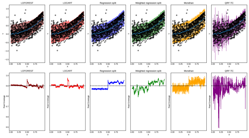
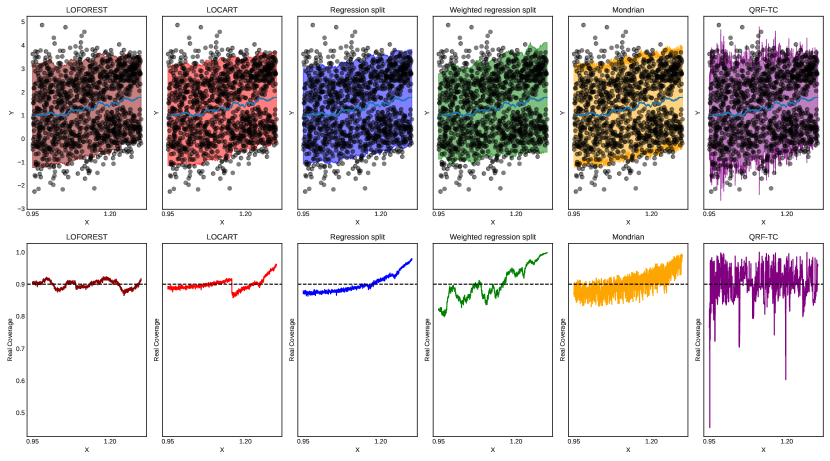
Figure 1: Top: failure of locally weighted regression split: the conditional mean absolute deviation of $[Y-\hat{\mu}(X)]$ is constant, but the conditional quantiles of $|Y-\hat{\mu}(X)|$ are not. Bottom: failure of using “difficulty” as the conditional variance of $Y$: the conditional variance $\mathbb{V}(Y|X=x)$ is constant, but the conditional quantiles of $|Y-\hat{\mu}(X)|$ are not. In both cases, the intervals do not adapt to the data’s local features and would fail to guarantee asymptotic conditional coverage. Our methods (Locart and Loforest), however, have good performance.

1.3 Notation and Organization

For an integer $n\geq 1$, we write $[n]$ to denote the set $\{1,\dots,n\}$. We will denote by $\sqcup$ the union of disjoint sets. We use $\mathbbm{1}\{\cdot\}$ for the indicator function. In addition, we denote by $\hat{q}_{\phi}(A)$ the empirical $\phi$-quantile of the set $A=\{a_{1},\dots,a_{n}\}$; that is,

$$\hat{q}_{\phi}(A)=\inf\left\{t:\frac{1}{n}\sum_{i=1}^{n}\mathbbm{1}\{a_{i}\leq t\}\geq\phi\right\}.$$

The remainder of the paper is organized as follows. We give an overview of Conformal Inference and Regression Trees/Forests in Section 2. In Section 3 we introduce our methods, discussing their properties and theoretical guarantees. In Section 4, we validate our approach in simulated and real-world datasets, comparing it to baselines. We conclude with a brief discussion in Section 5. All proofs are deferred to B.

2 Preliminaries

2.1 Conformal Inference

The main ingredient of the conformal inference framework is the conformity score $\hat{s}:{\mathcal{X}}\times{\mathcal{Y}}\to\mathbb{R}$, which measures how well the outputs of a regression or classification model accurately predict new labels $Y\in{\mathcal{Y}}$. In the regression setting, given an estimator $\hat{\mu}(\cdot)$ of the regression function $\mathbb{E}[Y|\mathbf{X}=\mathbf{x}]$, a standard choice is the regression residual $\hat{s}(\mathbf{x},y)=|y-\hat{\mu}(\mathbf{x})|$. Similarly, for the classification setting, given an estimator $\hat{\pi}_{Y}(\mathbf{x})$ of the true class probabilities $\pi_{Y}(\mathbf{x})$, one can use the generalized inverse quantiles from adaptive prediction sets (Romano et al., 2020) or its regularized version (Angelopoulos et al., 2020). In what follows, to avoid unnecessary restriction to either regression or classification, we let the underlying predictive model implicit in the choice of the conformity score. In this sense, “training” a conformal score refers to training this underlying predictive model and plugging it into the definition of the chosen conformity score.

A general method for obtaining prediction intervals in conformal inference with distribution-free guarantees is the split conformal prediction (split CP) framework (Papadopoulos et al., 2002; Vovk et al., 2005). Considering $\{(\mathbf{X}_{i},Y_{i})\}_{i=1}^{n+1}$ to be exchangeable data, split CP works as follows:

1. Split the data indices into two non-empty disjoint sets $I_{\textrm{train}}$ and $I_{\textrm{cal}}$, such that $I_{\textrm{train}}\sqcup I_{\textrm{cal}}=[n]$.

2. Train a conformity score $\hat{s}:{\mathcal{X}}\times{\mathcal{Y}}\to\mathbb{R}$ on $\{(\mathbf{X}_{i},Y_{i})\}_{i\in I_{\textrm{train}}}$.

3. Evaluate $\hat{s}(\mathbf{X}_{i},Y_{i})$ for all $i\in I_{\textrm{cal}}$.

4. Calculate $s^{*}$ as the empirical $\left(1+1/n_{\textrm{cal}}\right)(1-\alpha)$-quantile of $\hat{s}_{i}=\hat{s}(\mathbf{X}_{i},Y_{i})$ for $i\in I_{\textrm{cal}}$, where $n_{\textrm{cal}}$ is the size of $I_{\textrm{cal}}$.

5. For the new instance $(\mathbf{X}_{n+1},Y_{n+1})$, define the split conformal prediction set as

   $$C_{\textrm{split}}(\mathbf{X}_{n+1})=\{y\in{\mathcal{Y}}:\hat{s}(\mathbf{X}_{n+1},y)\leq s^{*}\}.$$ (1)

Because of the exchangeability of the data, the splitting step guarantees that the scores $\hat{s}_{i}$ for $i\in I_{\textrm{cal}}\sqcup\{n+1\}$ are also exchangeable. As a consequence, the rank of $\hat{s}(\mathbf{X}_{n+1},Y_{n+1})$ among these $n+1$ conformity scores is drawn uniformly from the $n+1$ possible indices. By choosing a cutoff $s^{*}$ as the empirical $\left(1+1/n_{\textrm{cal}}\right)(1-\alpha)$-quantile of the scores, we get that $\mathbb{P}[Y_{n+1}\in C_{\textrm{split}}(\mathbf{X}_{n+1})]=\mathbb{P}[\hat{s}(\mathbf{X}_{n+1},Y_{n+1})\leq s^{*}]\geq 1-\alpha$. The following theorem formalizes this explanation. Furthermore, it asserts that conditional on the training data (used to construct $\hat{s}$) and on average over all possible calibration datasets with $n_{\textrm{cal}}$ elements, the prediction band $C_{\textrm{split}}$ is not too wide provided $n_{\textrm{cal}}$ is sufficiently large. (See (Vovk, 2012; Bian and Barber, 2023) for guarantees incorporating the randomness of both the training and calibration datasets).

Theorem 1 (Lei et al., 2018).

Given an exchangeable sequence $(\mathbf{X}_{i},Y_{i})_{i=1}^{n+1}$ and a miscoverage level $\alpha\in(0,1)$,

$$\mathbb{P}[Y_{n+1}\in C_{\textrm{split}}(\mathbf{X}_{n+1})]\geq 1-\alpha,$$

where $C_{\textrm{split}}$ is the prediction band from the split conformal framework (1). In addition, if the conformal scores are almost surely distinct, then

$$\mathbb{P}[Y_{n+1}\in C_{\textrm{split}}(\mathbf{X}_{n+1})]\leq 1-\alpha+\frac{1}{n_{\textrm{cal}}+1}.$$

The split conformal framework can be naturally extended to produce prediction bands with local validity (Vovk et al., 2005; Lei and Wasserman, 2014). Let ${\mathcal{A}}=\{A_{1},\dots,A_{K}\}$ be a finite partition of the feature space and consider $\mathcal{T}:{\mathcal{X}}\to{\mathcal{A}}$ the function that maps $\mathbf{X}$ to the partition element it belongs. The extension works as follows: given the initial split $I_{\textrm{train}}$ and $I_{\textrm{cal}}$, we further split $I_{\textrm{cal}}$ into the sets $I_{j}=\{i\in I_{\textrm{cal}}:\mathcal{T}(\mathbf{X}_{i})=A_{j}\}$ for $j=1,\dots,K$. As before, the splitting step guarantees that the scores $\hat{s}_{i}$ for $i\in I_{j}\sqcup\{n+1\}$ are exchangeable. In complete analogy to split CP, for each split $I_{j}$, we calculate $s^{*}_{j}$ as the empirical $(1+1/n_{j})(1-\alpha)$-quantile of the scores $\hat{s}_{i}$ for $i\in I_{j}$, where $n_{j}$ is the size of $I_{j}$. Thus, we obtain that $\mathbb{P}[Y_{n+1}\in C_{\textrm{local}}(\mathbf{X}_{n+1})|\mathbf{X}_{n+1}\in A_{j}]\geq 1-\alpha$, where

$$C_{\textrm{local}}(\mathbf{X}_{n+1})=\{y\in{\mathcal{Y}}:\hat{s}(\mathbf{X}_{n+1},y)\leq s^{*}_{j}\}$$ (2)

is the local split conformal prediction set. If $I_{j}$ is an empty set, we take the convention that $s^{*}=+\infty$. Theorem 2 formalizes this discussion by stating the local validity of the prediction intervals (2).

Theorem 2.

Let ${\mathcal{A}}=\{A_{1},\dots,A_{K}\}$ be a finite partition of the feature space. Given an exchangeable sequence $(\mathbf{X}_{i},Y_{i})_{i=1}^{n+1}$ and a miscoverage level $\alpha\in(0,1)$,

$$\mathbb{P}[Y_{n+1}\in C_{\textrm{local}}(\mathbf{X}_{n+1})|\mathbf{X}_{n+1}\in A_{j}]\geq 1-\alpha,$$

for all $j=1,\dots,K$, where $C_{\textrm{local}}$ is the prediction band in (2).

Applying the split CP framework to each partition element entails a cost. If partition elements’ are not well-populated, prediction intervals grow wide. To see this, suppose we are given a realization of the dataset. If $\alpha=0.05$, then any partition element containing less than $\bar{n}=19$ instances will have trivial local bands, with $C_{\textrm{local}}(\cdot)=\mathbb{R}$. Therefore, the extension of split CP that attains local validity must be combined with a partition of the feature space whose elements are guaranteed to contain sufficiently many instances of the calibration split.

2.2 Regression Trees

Suppose we want to create an estimator $\hat{\mu}(\mathbf{x})$ of the regression function $\mathbb{E}[Y|\mathbf{X}=\mathbf{x}]$ given access to i.i.d samples $\{(\mathbf{X}_{i},Y_{i})\}_{i=1}^{n}$. Regression trees builds $\hat{\mu}$ by partitioning the feature space ${\mathcal{X}}$ in sets of the form $\{X_{j}\leq\ell\}$ and $\{X_{j}>\ell\}$, where $X_{j}$ is a feature and $\ell$ is a level. The splitting features and levels are chosen to minimize the sample variance of $Y$ inside each partition element. However, a “global” partitioning strategy is unfeasible due to the combinatorial hardness of testing all possible combinations of splitting features and levels. Instead, the partition is chosen by optimizing a greedy or local objective.

A standard way to greedily grow the tree is through the CART methodology (Breiman, 1993). Given a node t, starting from $\textup{{t}}=\textup{{t}}_{1}={\mathcal{X}}$ in the first step, the CART algorithm operates as follows:

1. Consider the left and right splits of t,

   $$\textup{{t}}_{L}(j,\ell)=\{\mathbf{X}\in\textup{{t}}:X_{j}\leq\ell\}\quad\textrm{and}\quad\textup{{t}}_{R}(s,\ell)=\{\mathbf{X}\in\textup{{t}}:X_{j}>\ell\}.$$

2. Determine the split $(\hat{\jmath},\hat{\ell})$ such that

   $$\frac{1}{N(\textup{{t}})}\Biggl{(}\sum\limits_{\mathbf{X}_{i}\in\textup{{t}}_{L}}(Y_{i}-\overline{Y}_{\textup{{t}}_{L}})^{2}+\sum_{\mathbf{X}_{i}\in\textup{{t}}_{R}}(Y_{i}-\overline{Y}_{\textup{{t}}_{R}})^{2}\Biggr{)}$$

   is minimized, where $N(\textup{{t}})=|\{\mathbf{X}\in\textup{{t}}\}|$ and $\overline{Y}_{\textup{{t}}}=\frac{1}{N(\textup{{t}})}\sum_{\mathbf{X}_{i}\in\textup{{t}}}Y_{i}$.

3. Recurse the procedure on $\textup{{t}}_{L}$ and $\textup{{t}}_{R}$ until the maximum depth $K$ is reached or some other stopping criterion is satisfied.

If the maximum depth $K$ of the tree is set to a high value, trees may overfit. This occurs after successive splittings of the training data since each terminal node of a tree may contain a single data instance. To avoid this, the tree may be pruned as the training unrolls or afterward. In the former case, called pre-pruning, the growth of the tree is controlled by setting the minimal amount of samples in each of its internal or terminal nodes (via the min_samples_split and min_samples_leaf hyperparameters, respectively, in the scikit-learn (Pedregosa et al., 2011) implementation). In the latter case, called post-pruning, subtrees or nodes are removed until a balance between model complexity and predictive performance is reached.

After training and pruning, the tree has a set of terminal nodes (or leaves) $\tilde{T}$ that can be naturally identified as a partition of the feature space. With this, define $\mathcal{T}:{\mathcal{X}}\to\tilde{T}$ as the function that maps a new instance $\mathbf{x}_{n+1}\in{\mathcal{X}}$ to the terminal node (partition element) it belongs. Then, the regression function estimate at $\mathbf{x}_{n+1}$ is $\hat{\mu}(\mathbf{x}_{n+1})=\overline{Y}_{\mathcal{T}(\mathbf{x}_{n+1})}$. It is also possible to view this estimate as a weighted nearest-neighbor method (Lin and Jeon, 2006); defining the weighting function

$$w_{i}(\mathbf{x})=\frac{\mathbbm{1}\{\mathbf{X}_{i}\in\mathcal{T}(\mathbf{x})\}}{N(\mathcal{T}(\mathbf{x}))},$$

the regression function estimate can be rewritten as

$$\hat{\mu}(\mathbf{x}_{n+1})=\sum_{i=1}^{n}w_{i}(\mathbf{x}_{n+1})Y_{i},$$

which highlights the data-adaptive nature of regression trees since the weight function is higher for the training points closer to the new instance $\mathbf{x}_{n+1}$. This property allows one to construct tree-based estimators of quantities beyond the conditional mean (Cevid et al., 2022). Indeed, Meinshausen (2006) shows that, under some mild assumptions, the function

$$\hat{F}(y|\mathbf{X}=\mathbf{x}_{n+1})=\sum_{i=1}^{n}w_{i}(\mathbf{x}_{n+1})\mathbbm{1}\{Y_{i}\leq y\}$$ (3)

is a consistent estimator of the conditional distribution $Y|\mathbf{X}=\mathbf{x}$ for all $\mathbf{x}\in{\mathcal{X}}$. Although the rate of convergence of $\hat{F}$ to the true distribution function might be possibly improved by bagging multiple trees, as done in Quantile Regression Forests (Meinshausen, 2006), the consistency holds even for a single tree. We will explore this fact to show the asymptotic conditional coverage property of Locart.

3 Methodology

In this section, we introduce our procedures for calibrating predictive intervals. First, building on the construction of the oracle prediction interval, we present an optimal partitioning scheme for local conformal. Then, we propose Local Coverage Regression Trees (Locart) as a realization of this scheme. Next, we introduce Local Coverage Regression Forests (Loforest), which is a non-conformal alternative to Locart based on averaging cutoff estimates that exhibit improved empirical performance. Then, we introduce the augmented versions of both algorithms, A-Locart and A-Loforest, that can further refine the partitions by augmenting the feature space. Finally, we present a weighted version of Loforest called W-Loforest that can be used to improve the locally weighted prediction intervals (Lei et al., 2018).

3.1 Motivation

We consider prediction sets of the form

$$C(\mathbf{x})=(\hat{\mu}(\mathbf{x})-\hat{t}_{1-\alpha}(\mathbf{x}),\hat{\mu}(\mathbf{x})+\hat{t}_{1-\alpha}(\mathbf{x})).$$

Ideally, we would like to choose the cutoff $\hat{t}_{1-\alpha}$ such that, for a fixed miscoverage level $\alpha\in(0,1)$, the prediction set $C(\mathbf{x})$ controls conditional coverage. The prediction set that uses this optimal cutoff is named the oracle prediction interval:

Definition 1 (Oracle prediction interval).

Given a regression estimator $\hat{\mu}$, the oracle prediction interval $C^{*}(\mathbf{x})$ is defined as

$$C^{*}(\mathbf{x}):=(\hat{\mu}(\mathbf{x})-t_{1-\alpha}^{*}(\mathbf{x}),\hat{\mu}(\mathbf{x})+t_{1-\alpha}^{*}(\mathbf{x})),$$

where $t_{1-\alpha}^{*}(\mathbf{x})$ is the $(1-\alpha)$-quantile of the regression residual $\hat{s}(\mathbf{X},Y)=|Y-\hat{\mu}(\mathbf{X})|$ conditional on $\mathbf{X}=\mathbf{x}$. This is the only symmetric interval around $\hat{\mu}(\cdot)$ such that

$$\mathbb{P}[Y\in C^{*}(\mathbf{X})|\mathbf{X}=\mathbf{x},\hat{\mu}]=1-\alpha.$$

It is of course impossible to obtain $t^{*}_{1-\alpha}$ in practice. Our goal is, therefore, to get as close as possible to $t^{*}_{1-\alpha}$. We will do this by calibrating the cutoff $\hat{t}_{1-\alpha}(\mathbf{x})$ using a local conformal approach.

To recover $t^{*}_{1-\alpha}$ effectively, the partition ${\mathcal{A}}$ must be designed such that all $\mathbf{x}$ values within the same element $A\in{\mathcal{A}}$ (approximately) share the same optimal cutoff. This is because a local conformal method, by design, will yield the same cutoff for all $\mathbf{x}$ values belonging to the same element $A\in{\mathcal{A}}$. In other words, if $A$ is such that all $\mathbf{x}\in A$ approximately share the same $t^{*}_{1-\alpha}$, then

$$\mathbb{P}[Y\in C(\mathbf{X})|\mathbf{X}=\mathbf{x},\hat{\mu}]\approx\mathbb{P}[Y\in C(\mathbf{X})|\mathbf{X}\in A,\hat{\mu}]=1-\alpha,$$

that is, the local conformal intervals $C(\mathbf{X})$ will not only have local coverage but will also be close to conditional coverage.

Euclidean partitions are one approach that aims to achieve this objective (Lei and Wasserman, 2014): as $\text{dim}(A)\longrightarrow 0$, $A$ will only have a single point $\mathbf{x}$, and therefore all elements of $A$ will share the same optimal cutoff. Euclidean partitions, however, are not optimal: two $\mathbf{x}$’s may be far from each other but still share the same optimal cutoff, as the next examples show:

Example 1.

[Location family] Let $h(y)$ be a density, $\mu(\mathbf{x})$ a function, and $Y|\mathbf{x}\sim h(y-\mu(\mathbf{x}))$. In this case, $t^{*}_{1-\alpha}(\mathbf{x}_{a})=t^{*}_{1-\alpha}(\mathbf{x}_{b})$, for every $\mathbf{x}_{a},\mathbf{x}_{b}\in\mathbb{R}^{d}$. For instance, if $Y|\mathbf{x}\sim N(\beta^{t}\mathbf{x},\sigma^{2})$, then all instances have the same optimal cutoff. Thus, in this special scenario, a unitary partition ${\mathcal{A}}=\mathcal{X}$ would already lead to conditional validity as the calibration sample increases.

Example 2.

[Irrelevant features] If $\mathbf{x}_{S}$ is a subset of the features such that the conditional densities satisfy $f(y|\mathbf{x})=f(y|\mathbf{x}_{S})$, then $t^{*}_{1-\alpha}(\mathbf{x})=t^{*}_{1-\alpha}(\mathbf{x}_{S})$, that is, the optimal cutoff does not depend on the irrelevant features, $S^{c}$. These irrelevant features, however, affect the Euclidean distance between $\mathbf{x}$’s.

Therefore, even if two $\mathbf{x}$ values are distant, they can still be included in the same $A$ if they share the same $t^{*}_{1-\alpha}(\mathbf{x})$. This is equivalent to saying that the optimal partition should group instances with the same conditional distribution of the residuals $\hat{s}(\mathbf{X},Y)|\mathbf{X}=\mathbf{x}$.

Theorem 3 formalizes the construction and optimality of such partition.

Theorem 3 (The coarsest partition with same oracle cutoffs).

Let $\mathcal{A}$ be a partition of ${\mathcal{X}}$ such that, for any $A\in\mathcal{A}$, $\mathbf{x}_{1},\mathbf{x}_{2}\in A$ if and only if $\hat{s}(\mathbf{X},Y)|\mathbf{X}=\mathbf{x}_{1}\sim\hat{s}(\mathbf{X},Y)|\mathbf{X}=\mathbf{x}_{2}$, where $\hat{s}(\mathbf{X},Y)=|Y-\hat{\mu}(\mathbf{X})|$. Let $t_{1-\alpha}^{*}(\mathbf{x})$ be $(1-\alpha)$-quantile of the regression residual, as in Definition 1. Then,

1. If $\mathbf{x}_{1},\mathbf{x}_{2}\in A$, then $t_{1-\alpha}^{*}(\mathbf{x}_{1})=t_{1-\alpha}^{*}(\mathbf{x}_{2})$ for every $\alpha\in(0,1)$

2. If $\mathcal{J}$ is another partition of ${\mathcal{X}}$ such that, for any $J\in\mathcal{J}$, $\mathbf{x}_{1},\mathbf{x}_{2}\in J$ implies that $t_{1-\alpha}^{*}(\mathbf{x}_{1})=t_{1-\alpha}^{*}(\mathbf{x}_{2})$ for every $\alpha\in(0,1)$, then

   $$\mathbf{x}_{1},\mathbf{x}_{2}\in J\implies\mathbf{x}_{1},\mathbf{x}_{2}\in A.$$

Locart attempts to recover the partition described in this theorem. We explore this approach in the next section.

3.2 Locart: Local Coverage Regression Trees

A regression tree naturally induces a partition of the feature space. Moreover, as discussed in Section 2.2, regression trees are consistent estimators of conditional distributions. Thus, a regression tree that predicts the residual $\hat{s}(\mathbf{X},Y)$ using $\mathbf{x}$ as an input attempts to recover the partition described by Theorem 3, that is, the partition that groups features according to the conditional distribution of the residuals. This is, therefore, how Locart builds the partition ${\mathcal{A}}$. We detail Locart’s algorithm and practical considerations in Section 3.2.1 and formalize its theoretical properties in Section 3.2.2.

3.2.1 The algorithm

Given a regression estimator $\hat{\mu}(\cdot)$ trained on $\{(\mathbf{X}_{i},Y_{i})\}_{i\in I_{\textrm{train}}}$ and the calibration split with indices $I_{\textrm{cal}}$, Locart consists of four steps, as outlined in 2:

1. Obtain the regression residuals $\hat{s}_{i}$ of $\hat{\mu}$ on $I_{\textrm{cal}}$, that is, compute $\hat{s}_{i}=\hat{s}(\mathbf{X}_{i},Y_{i})=|\hat{\mu}(\mathbf{X}_{i})-Y_{i}|$, for every $i\in I_{\textrm{cal}}$.

2. Create the dataset $\{(\mathbf{X}_{i},\hat{s}_{i})\}_{i\in I_{\textrm{cal}}}$ of pairs of features and regression residuals computed on the calibration dataset, and split it into two disjoint sets $I_{\textrm{part}}$ and $I_{\textrm{cut}}$.

3. Fit a regression tree on $\{(\mathbf{X}_{i},\hat{s}_{i})\}_{i\in I_{\text{part}}}$ that predicts the residuals $\hat{s}$ based on the features $\mathbf{X}$. This tree induces a partition ${\mathcal{A}}$ of the feature space generated by its terminal nodes, as discussed in Section 2. Let $\mathcal{T}:{\mathcal{X}}\to{\mathcal{A}}$ be the function mapping an element of ${\mathcal{X}}$ to the partition element it belongs.

4. Estimate $\hat{t}_{1-\alpha}(\mathbf{x}_{n+1})$ for a new instance $\mathbf{x}_{n+1}$ by applying the conformal approach to all instances in $\{(\mathbf{X}_{i},s_{i})\}_{i\in I_{\text{cut}}}$ that fall into the same element of ${\mathcal{A}}$ as $\mathbf{x}_{n+1}$ does. That is, we estimate $\hat{t}_{1-\alpha}(\mathbf{x}_{n+1})$ as

   $$\hat{t}_{1-\alpha}(\mathbf{x}_{n+1})=\hat{q}_{1-\alpha}(A(\mathbf{x}_{n+1}))$$ (4)

   where

   $$A(\mathbf{x}_{n+1})=\left\{\hat{s}_{i}:\mathcal{T}(\mathbf{x}_{i})=\mathcal{T}(\mathbf{x}_{n+1}),(\mathbf{X}_{i},\hat{s}_{i})\in\{(\mathbf{X}_{i},\hat{s}_{i})\}_{i\in I_{\text{cut}}}\right\}.$$ (5)

5. Using $\hat{t}_{1-\alpha}(\mathbf{x}_{n+1})$ from Equation 4, define the Locart prediction interval as

   $$C_{\textup{{Locart}}{}}(\mathbf{x})=(\hat{\mu}(\mathbf{x})-\hat{t}_{1-\alpha}(\mathbf{x}),\hat{\mu}(\mathbf{x})+\hat{t}_{1-\alpha}(\mathbf{x})).$$

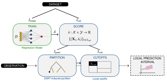
Figure 2: Schematic diagram of Locart. Train: a regression model (e.g., neural network) is fitted on the $I_{\textrm{train}}$ split, producing the estimator $\hat{\mu}$. Score: the regression residuals are calculated on $I_{\textrm{cal}}$ and a new dataset of features and residuals produced. This dataset is split into $I_{\textrm{part}}$, used to create a partition of the feature space by fitting a regression tree of residuals, and $I_{\textrm{cut}}$, used to populate this partition and calculate cutoffs that calibrate prediction intervals locally. In each partition element, the residuals are (approximately) uniformly distributed. As a result, the local thresholds computed in each leaf will converge to the oracle threshold in the asymptotic regime. The path of a new observation ( ): the partition element it belongs to is identified; then, the local cutoff is retrieved; next, this cutoff is used to create an adaptive interval centered at the prediction of the regression model for this observation.

When using the regression tree algorithm to partition, we may need to control tree growth to avoid empty or redundant partitions. To do that, we perform pre and post-pruning. The pre-pruning is done by fixing the min_samples_split hyperparameter in values such as 100 samples, which enables us to obtain well-populated partitions/leaves resulting in accurate cutoff estimations. For the post-pruning step, we remove extra leaves and nodes via cost-complexity pruning (as implemented in the scikit-learn library) until we balance partition complexity and predictive performance, reducing the amount of less informative partition elements.

The remaining regression tree hyperparameters are fixed at scikit-learn’s defaults. As a result, we can construct our flexible and adaptive partitions without hyperparameter tuning, which requires multiple refits and could drastically increase the algorithm’s running time. Plus, as we make use of the scikit-learn’s efficient CART implementation, Locart often outperforms benchmarks in the run-time comparison (see Section 4). It is also worth noticing that, to increase Locart’s power and circumvent sample size reduction in the calibration step, the splitting of the calibration set presented in Step 2 can be skipped, as it is only necessary to derive the theoretical properties explored in Section 3.2.2. The empirical results in Section 4 reinforce this observation, as Locart presents good performances without splitting the calibration set.

3.2.2 Theoretical properties

By construction of the algorithm, if we fix the partition index set $I_{\textrm{part}}$, Locart produces a fixed partition ${\mathcal{A}}$ of the feature space, and thus, satisfies Theorem 2 (i.e., it is locally valid). Consequently, it also satisfies marginal validity. Corollaries 1 and 2 formalize both statements:

Corollary 1 (Local coverage property of Locart).

Given an i.i.d. sequence $(\mathbf{X}_{i},Y_{i})_{i=1}^{n+1}$ and a fixed partition ${\mathcal{A}}$ of the feature space ${\mathcal{X}}$ induced by Locart using $I_{\textrm{part}}$, the predictive intervals of Locart satisfy:

$$\mathbb{P}[Y_{n+1}\in C_{\textup{{Locart}}{}}(\mathbf{X}_{n+1})|\mathbf{X}_{n+1}\in A,I_{\textrm{part}},I_{\textrm{train}}]\geq 1-\alpha,$$

for all $A\in{\mathcal{A}}$.

Corollary 2 (Marginal coverage property of Locart).

Given an exchangeable sequence $(\mathbf{X}_{i},Y_{i})_{i=1}^{n+1}$, the predictive intervals of Locart satisfy:

$$\mathbb{P}[Y_{n+1}\in C_{\textup{{Locart}}{}}(\mathbf{X}_{n+1})|I_{\textrm{train}}]\geq 1-\alpha.$$

Also, notice that the Locart cutoff $\hat{t}_{1-\alpha}(\mathbf{x}_{n+1})$ can be written as the inverse of the conditional distribution estimator from Equation 3 at level $1-\alpha$, that is:

$$\hat{t}_{1-\alpha}(\mathbf{X}_{n+1})=\hat{F}^{-1}(1-\alpha|\mathbf{X}_{n+1})\;.$$ (6)

Thus, it is intuitive to think that, by the consistency of regression trees as conditional distribution estimators (Meinshausen, 2006), the Locart cutoff will be close to the oracle cutoff as sample size increases. Indeed, under additional assumptions about the partition’s scheme and conditional cumulative distribution, Locart converges to the oracle prediction interval on the asymptotic regime.

To show this, we first assume that asymptotically: (i) the partition elements’ are well-populated and (ii) the partition is sufficiently thin:

Assumption 1.

Let $A_{n}(\mathbf{x})$, denote the Locart partition element assigned to $\mathbf{x}$, as in Equation 5, when $I_{cut}$ has size $n$. Then,

$$\lim_{n\rightarrow\infty}\inf_{\mathbf{x}\in{\mathcal{X}}}n\cdot\mathbb{P}[A_{n}(\mathbf{x})]>0.$$

Also, we assume that the partition-based $1-\alpha$ quantile of the conditional distribution of $Y$ is close to the $1-\alpha$ quantile of the true conditional distribution of $Y$ given $\mathbf{X}$:

Assumption 2.

Let $F_{\mathbf{x}}(y|\mathbf{X}_{i})\coloneqq\mathbb{P}[Y_{i}\leq y|\mathbf{X}_{i}\in A_{n}(\mathbf{x})]$. For every $\mathbf{x}$, $F_{\mathbf{x}}$ is continuous and increasing in a neighborhood around $F^{-1}(1-\alpha|\mathbf{x})$ and $\sup_{\mathbf{x}\in{\mathcal{X}}}|F^{-1}_{\mathbf{x}}(1-\alpha|\mathbf{X}_{i})-F^{-1}(1-\alpha|\mathbf{x})|=o_{\mathbb{P}}(1)$.

Under both assumptions, Locart converges to the oracle prediction interval in Theorem 4:

Theorem 4 (Consistency of Locart).

Let $(\mathbf{X}_{i},Y_{i})_{i=1}^{n+1}$ be an i.i.d sequence. Consider $\hat{t}_{1-\alpha}(\mathbf{X}_{n+1})$ and $t_{1-\alpha}^{*}(\mathbf{X}_{n+1})$ the Locart cutoff estimate and the oracle cutoff for the test point $\mathbf{X}_{n+1}$. Then, under Assumptions 1 and 2 , $|t^{*}(\mathbf{X}_{n+1})-\hat{t}_{1-\alpha}(\mathbf{X}_{n+1})|=o_{\mathbb{P}}(1)$.

Finally, by using Theorem 4 in the asymptotic regime, we show that Locart satisfies asymptotic conditional validity, as formalized in Theorem 5.

Theorem 5 (Asymptotic conditional validity of Locart).

Let $(\mathbf{X}_{i},Y_{i})_{i=1}^{n+1}$ be an i.i.d sequence. Under Assumptions 1 and 2, Locart satisfies asymptotic conditional validity.

3.3 Loforest: Local Coverage Regression Forest

Regression trees have difficulty in modeling some functional relationships such as additive structures (Hastie et al., 2009). Thus, Locart may yield suboptimal results in datasets where regression residuals exhibit such behavior. Moreover, given the decision tree partition structure, Locart may also provide poor cutoff estimates for instances in the boundaries of its partition elements. Loforest improves Locart by drawing upon the success of Random Forests. It seeks to increase the expressivity of Locart and provides smoother cutoff estimates. Concretely, Loforest builds several partitions ${\mathcal{A}}_{k}$ by fitting many decision trees to bootstrap samples (one for each tree) of the original residuals and features in the calibration set. Let $B$ be the number of created decision trees. Loforest, as depicted in Figure 3, consists of five steps:

1. Obtain the regression residuals $\hat{s}_{i}$ of $\hat{\mu}$ on $I_{\textrm{cal}}$, that is, compute $\hat{s}_{i}=\hat{s}(\mathbf{X}_{i},Y_{i})=|\hat{\mu}(\mathbf{X}_{i})-Y_{i}|$, for every $i\in I_{\textrm{cal}}$.

2. Create the dataset $\{(\mathbf{X}_{i},s_{i})\}_{i\in I_{\textrm{cal}}}$ of pairs of features and regression residuals computed on the calibration dataset, and randomly split it into two disjoint sets $I_{\textrm{part}}$ and $I_{\textrm{cut}}$.

3. Fit a Random Forest on $\{(X_{i},s_{i})\}_{i\in I_{part}}$, which predicts the residuals $\hat{s}$ based on the features $\mathbf{X}$. This algorithm induces several partitions of the feature space ${\mathcal{A}}_{j}$, $j=1,\dots,B$, using the decision tree algorithm on each of the $B$ bootstrap samples.

4. For a new instance $\mathbf{x}_{n+1}$, estimate the local cutoff $\hat{t}_{1-\alpha}^{(k)}(\mathbf{x}_{n+1})$ in each decision tree the same way as done in the Locart algorithm, using the dataset $\{(\mathbf{X}_{i},s_{i})\}_{i\in I_{cut}}$.

5. Compute the final cutoff $\hat{t}_{1-\alpha}(\mathbf{x}_{n+1})$ by averaging all the cutoffs obtained in each decision-tree partition ${\mathcal{A}}_{k}$:

   $$\widehat{t}_{1-\alpha}(\mathbf{x}_{n+1}):=\frac{1}{n}\sum_{k=1}^{B}\widehat{t}_{1-\alpha}^{(k)}(\mathbf{x}_{n+1}).\;$$ (7)

6. Using $t_{1-\alpha}(\mathbf{x}_{n+1})$ from Equation 7, define the Loforest prediction interval as

   $$C_{\textup{{Loforest}}{}}(\mathbf{x})=(\hat{\mu}-\widehat{t}_{1-\alpha}(\mathbf{x}),\hat{\mu}+\widehat{t}_{1-\alpha}(\mathbf{x})).$$

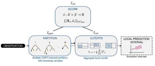
Figure 3: Schematic diagram of Loforest, as a modification of the scoring procedure of Locart. The regression residuals are calculated on $I_{\textrm{cal}}$, and a new dataset of features and residuals is produced. This dataset is split into $I_{\textrm{part}}$, used to create multiple partitions (each one associated with a bootstrap sample of $I_{\textrm{part}}$) of the feature space by fitting a Random Forest of residuals, and $I_{\textrm{cut}}$, used to populate these partitions and calculate the cutoffs for each tree. The path of a new observation ( ): all the partition elements it belongs to are identified; then, the local cutoffs for each partition are retrieved; next, an average of all the cutoffs is used to create an adaptive interval centered at the prediction of the regression model for this observation. As a result of the averaging step, these intervals are smoother than their Locart counterparts.

As in Locart, to obtain meaningful local cutoffs in each decision tree, it is essential to control each decision tree growth by either pre or post-pruning. Nevertheless, post-pruning can become computationally expensive if applied to all bootstrap trees. Most importantly, it can diminish the variability between the decision trees and undermine the benefit of ensembling different partitions induced by the Random Forest ensemble. Thus, for Loforest, we only apply a pre-pruning step in the same way as in Section 3.2.1, fixing the min_samples_split hyperparameter in values such as 100 samples. For the remaining Random Forest hyperparameters, we set the number of trees as 100.

Our implementation of Loforest uses the scikit-learn Random Forest implementation and, as a consequence, is scalable, as shown in the benchmarking studies in Section 4. Similarly to Locart, empirical results attest that we can skip splitting the calibration set presented in step 2 without harming the method’s performance. The results presented in Section 4 show that Loforest outperforms several baselines with respect to conditional and marginal coverage of its intervals in benchmark datasets.

3.4 A-Locart and A-Loforest: augmenting the feature space

In Sections 3.2 and 3.3, we discuss how Locart and Loforest obtain prediction intervals by partitioning the feature space. Such strategies aim to recover the optimal partition from Theorem 3, which groups each sample according to the conditional distribution of residuals. In both methods, we only use the original features to create one or several partitions of the feature space.

The idea of the augmented versions of these methods, A-Locart and A-Loforest, is to improve the partitioning by providing additional statistics (i.e., other functions of the features) as inputs of the trees. One possible way of doing this is by giving first-order proxies to the conditional distribution of residuals. This can be done by using an estimate of $\mathbb{V}[Y|\mathbf{X}]$, for example. Notice that using $\widehat{\mathbb{V}}[Y|\mathbf{X}]$ as a feature is closely connected to the approach adopted in Mondrian Conformal Regressors (Vovk et al., 2005; Boström and Johansson, 2020). In fact, by using conditional variance estimates as new covariates, we generalize the Mondrian taxonomy by expanding the binning based on $\mathbb{V}[Y|\mathbf{X}]$ to a general partitioning of both $\mathbb{V}[Y|\mathbf{X}]$ and ${\mathcal{X}}$. This avoids the need to tune or fix the number of bins, as we use Locart and Loforest engines to obtain the partitions. Moreover, it also avoids the adversarial setting for the vanilla Mondrian approach where the variance is constant, but the conditional quantiles of residuals are not (as discussed in Section 1 and expanded in A).

In general, we may also add as features of our model other proxies for the distribution of the residuals (e.g., their conditional mean absolute deviation, as used by Lei et al. (2018)) or new feature representations (e.g., random Fourier features (Rahimi and Recht, 2007) and random projections (Fradkin and Madigan, 2003)). Section 4 illustrates how the augmentation procedure can improve Locart and Loforest partitioning.

3.5 Extensions to other conformal scores and W-Loforest

In the previous sections, we focused on partitioning ${\mathcal{X}}$ based on the regression residuals. However, as introduced in Section 2.1, this is a particular choice of conformity score. In some cases, it is preferable to build locally valid prediction intervals based on other conformity scores, such as the quantile score and the weighted regression score, mainly when performing inferential tasks other than regression (e.g., quantile regression, conditional distribution estimation).

The Locart and Loforest frameworks can be straightforwardly generalized to accommodate any of these situations since these methods are completely agnostic to the choice of conformity score. Even the theoretical guarantees for Locart are not directly tied to the regression residual and naturally extend to other conformity scores. In Section 4, we showcase the benefits of using the weighted regression score of Lei et al. (2018) within Loforest, an approach we call W-Loforest.

4 Experiments

In this section, we compare the conditional coverage performance of Locart, A-Locart, Loforest, A-Loforest and W-Loforest to other state-of-the-art methods for conformal regression and regression intervals on simulated and real-world datasets.

We use Random Forests as the base model for estimating $\hat{\mu}(\cdot)$ across all methods. We set n_estimators to 100, i.e., predictions are averaged over 100 trees. We set a common miscoverage level for predictive intervals at $\alpha=0.1$. We compare our methods against the following baselines:

• Regression split (Vovk et al., 2005; Lei et al., 2018): implemented in the nonconformist library (Linusson et al., 2021). The only hyperparameter is the miscoverage level.

• Weighted regression split (Lei et al., 2018): implemented in our library, clover. We use a Random Forest regressor to estimate the mean absolute deviation of the residuals. The only hyperparameter is the miscoverage level.

• Mondrian split (Boström and Johansson, 2020): implemented in our library, clover. We use the default difficulty estimator (variance of predictions across trees in the Random Forest). Difficulty estimates were binned in $k=30$ groups according to the quantiles $(1/k,2/k,\dots,\frac{k-1}{k},1)$.

• QRF-TC (Amoukou and Brunel, 2023; Guan, 2021): implemented in the acpi library (Amoukou and Brunel, 2023). We set the calibration model as a Random Forest Regressor with 100 trees, a minimal node size of 10, a maximum tree depth of 15, and squared error as the split criterion.

To evaluate the conditional validity of intervals output by all methods, we employed the SMIS metric (Gneiting and Raftery, 2007) for real-world datasets and the conditional coverage absolute deviation for synthetic datasets. We also evaluated marginal validity by computing the average marginal coverage for all datasets. These metrics are briefly described in Section 4.1. We replicate the experiments 100 times and compute the average and standard error at the end to estimate the various measures of interest. To give a comprehensive analysis, we divide our evaluation into three parts: conformal methods only, non-conformal methods only, and a combined assessment of all methods. Additionally, we assess the running time of each method to compare their scalability.

4.1 Metrics for assessing marginal and conditional validity

In this section, we introduce the metrics used in the experiments. Here, we denote by $C(\cdot)$ any prediction interval and by $\{(\mathbf{x}_{i},y_{i})\}_{i\in I_{\textrm{test}}}$ a testing set used to compute coverage diagnostics for all compared methods.

4.1.1 Conditional coverage absolute deviation (CCAD)

In the simulation study, we know the ground truth distribution of $Y|\mathbf{X}$. Thus, we can directly measure the conditional coverage. We do this by evaluating the conditional coverage absolute deviation (CCAD): for each $i\in I_{\textrm{test}}$, we obtain a sample $\mathcal{D}=\{(\mathbf{x}_{i},Y_{1},\dots,\mathbf{x}_{i},Y_{B_{y}}\}$ of size $B_{y}$ (fixed as $1,000$) from $Y|\mathbf{X}=\mathbf{x}_{i}$ and compute

$$\delta_{\alpha}(\mathbf{x}_{i})=\frac{1}{B_{y}}\sum_{y\in\mathcal{D}}\mathbbm{1}\{y\in C(\mathbf{x}_{i})\}.$$

$\delta_{\alpha}(\mathbf{x}_{i})$ is an estimate of the conditional coverage $\mathbb{P}[Y\in C(\mathbf{X})|\mathbf{X}=\mathbf{x}_{i}]$. We derive the conditional coverage absolute deviation (CCAD) by averaging the absolute difference between $\delta_{\alpha}(\mathbf{x}_{i})$ and the nominal level $1-\alpha$ for all $i\in I_{\textrm{test}}$,

$$\textrm{CCAD}=\frac{1}{|I_{\textrm{test}}|}\sum_{i\in I_{\textrm{test}}}\left|\delta_{\alpha}(\mathbf{x}_{i})-(1-\alpha)\right|.$$ (8)

4.1.2 Standard Mean Interval Score (SMIS)

In real-world datasets, we cannot compute CCAD because the data-generating process is unknown. Instead, we use the standard mean interval score (SMIS) from Gneiting and Raftery (2007). The interval score associated with $y$ and the miscoverage level $\alpha$ is calculated as

$$\text{IS}_{\alpha}(C(\mathbf{x}),y)= \,(\max{C(\mathbf{x})}-\min{C(\mathbf{x}))}$$

$$+\frac{2}{\alpha}(\min{C(\mathbf{x})}-y)\mathbbm{1}\{y<\min{C(\mathbf{x})}\}$$

$$+\frac{2}{\alpha}(y-\max{C(\mathbf{x})})\mathbbm{1}\{y>\max{C(\mathbf{x})}\},$$ (9)

where $\min{C(\mathbf{x})}$ and $\max{C(\mathbf{x})}$ are the minimum and maximum of the (closed) prediction interval $C(\mathbf{x})$. Intuitively, the interval score penalizes large prediction intervals (first term) that do not contain $y$ (second and third terms) in proportion to how far $y$ is from the limits of the interval and the stricter the miscoverage level. In other words, this score prioritizes the narrowest valid (i.e., containing $y$) prediction interval. The standard mean interval score is then the average over the whole testing set $\{(\mathbf{X}_{i},Y_{i})\}_{i\in I_{\textrm{test}}}$:

$$\textrm{SMIS}_{\alpha}(C,\mathcal{D})=\frac{1}{|I_{\textrm{test}}|}\sum_{i\in I_{\textrm{test}}}\text{IS}_{\alpha}(C(\mathbf{X}_{i}),Y_{i})\;,$$ (10)

which gives us a general balance of interval length and coverage of $y$ for the prediction interval method $C$. Thus, it can be interpreted as an approximate measure of conditional coverage.

4.1.3 Average marginal coverage

We also estimate the average marginal coverage $\mathbb{P}[Y\in C(\mathbf{X})]$ using

$$\text{AMC}=\frac{1}{|I_{\textrm{test}}|}\sum_{i\in I_{\textrm{test}}}\mathbbm{1}\{y_{i}\in C(\mathbf{x}_{i})\}.$$ (11)

4.2 Simulated data performances

We adopt the simulated settings employed in Izbicki et al. (2022), incorporating some modifications to the number of noisy variables and introducing two additional scenarios. Let $\mathbf{X}=(X_{1},\dots,X_{d})$, where $X_{i}\overset{\text{i.i.d}}{\sim}\text{Unif}(-1.5,1.5)$, and $d$ and $p$ denotes the total number of features and relevant features respectively. The selected simulated settings are as follows:

• Homoscedastic:

  $$Y|\mathbf{x}\sim N\left(\frac{2}{p}\sum_{i=1}^{p}x_{i},1\right)$$

• Heteroscedastic:

  $$Y|\mathbf{x}\sim N\left(\frac{2}{p}\sum_{i=1}^{p}x_{i},0.25+2\left|\frac{1}{p}\sum_{i=1}^{p}x_{i}\right|\right)$$

• Asymmetric:

  $$Y|\mathbf{x}=\frac{2}{p}\sum_{i=1}^{p}x_{i}+\varepsilon,$$

  where $\varepsilon\sim\text{Gamma}\left(1+\gamma\left|\frac{\sum_{i=1}^{p}x_{i}}{p}\right|,1+\gamma\left|\frac{\sum_{i=1}^{p}x_{i}}{p}\right|\right)$, with $\gamma=0.6$ and $1.5$

• $t$-residuals:

  $$Y|\mathbf{x}=\frac{2}{p}\sum_{i=1}^{p}x_{i}+\varepsilon,$$

  where $\varepsilon\sim\text{t}_{4}$.

• Non-Correlated Heteroscedastic:

  $$Y|\mathbf{x}\sim N\left(1,0.25+\left|\frac{2}{p}\sum_{i=1}^{p}x_{i}\right|\right)$$

To enhance the diversity of simulated scenarios, we consider three values for the number of significant features $p$: $1,3$, and $5$ and fix $d$ as $20$ for all possible scenarios. For each value of $p$, we generate a total of 10,000 training and calibration samples and 5,000 testing samples.

In each run, we evaluate the performance of various methods by estimating the mean conditional coverage absolute deviation (CCAD) and the marginal coverage (AMC) associated with the predictive intervals. To determine these metrics, we employ a holdout testing set and measure the running time required for the calibration step for each method.

In general, all methods achieve marginal coverage levels that are very close to the nominal value of 90%, as shown in Table 4 (see C for details). However, when it comes to conditional coverage, Table 1 and Figure 4 indicate variations in performance across different methods:

• In both homoscedastic settings (homoscedastic and $t$-residuals), we observe in Table 1 that the regression split method demonstrates the best performance, closely followed by Locart and A-Locart. This is because the cutoff $\hat{t}_{1-\alpha}(\mathbf{x})$ remains constant for $\mathbf{x}$. Locart and A-Locart decision trees capture this behavior and reduce to a trivial tree with only one leaf, effectively replicating the regression split.

• In all other settings, particularly the asymmetric and heteroscedastic settings, our non-conformal methods (Loforest, A-Loforest) exhibit superior performance. Additionally, among the conformal methods, the first panel in Figure 4 and Table 1 demonstrate that our two conformal procedures also excel in these settings.

• QRF-TC does not perform as well as either the other non-conformal or conformal methods, as evident from Table 1 and the second and third panels in Figure 4.

• Considering a comprehensive analysis of all methods and settings, the third panel of Figure 4 indicates that our methods outperform all other regression interval methods.

Table 1: Mean conditional coverage absolute deviation (CCAD) values for each method and simulation setting. The average across 100 runs is reported with two times the standard error in brackets. Values in bold indicate the methods with better performance in a $95\%$ confidence interval. In general, our methods achieve the best performance in almost all datasets.

Dataset $p$ Type of method Conformal Non-conformal Locart A-Locart RegSplit W-RegSplit Mondrian Loforest A-Loforest W-Loforest QRF-TC Asym. 1 0.033 (0.0004) 0.036 (0.0004) 0.06 (0.0003) 0.042 (0.0002) 0.039 (0.0002) 0.028 (0.0002) 0.026 (0.0002) 0.039 (0.0002) 0.041 (0.0003) Asym. 3 0.046 (0.0007) 0.04 (0.0003) 0.051 (0.0003) 0.045 (0.0003) 0.041 (0.0003) 0.037 (0.0003) 0.036 (0.0002) 0.041 (0.0003) 0.049 (0.0005) Asym. 5 0.045 (0.0003) 0.04 (0.0003) 0.045 (0.0003) 0.046 (0.0003) 0.041 (0.0002) 0.039 (0.0002) 0.037 (0.0002) 0.043 (0.0003) 0.048 (0.0006) Asym. 2 1 0.04 (0.0005) 0.043 (0.0005) 0.086 (0.0003) 0.045 (0.0003) 0.041 (0.0002) 0.027 (0.0002) 0.028 (0.0002) 0.042 (0.0002) 0.049 (0.0004) Asym. 2 3 0.064 (0.0007) 0.055 (0.0003) 0.084 (0.0003) 0.055 (0.0003) 0.053 (0.0003) 0.048 (0.0003) 0.05 (0.0002) 0.051 (0.0003) 0.065 (0.0005) Asym. 2 5 0.072 (0.0004) 0.059 (0.0003) 0.073 (0.0003) 0.063 (0.0003) 0.058 (0.0002) 0.06 (0.0003) 0.054 (0.0002) 0.057 (0.0003) 0.068 (0.0005) Heterosc. 1 0.029 (0.0005) 0.032 (0.0004) 0.066 (0.0002) 0.041 (0.0001) 0.031 (0.0002) 0.017 (0.0002) 0.019 (0.0002) 0.04 (0.0001) 0.044 (0.0004) Heterosc. 3 0.054 (0.0006) 0.046 (0.0003) 0.069 (0.0002) 0.051 (0.0002) 0.043 (0.0002) 0.041 (0.0003) 0.041 (0.0001) 0.049 (0.0002) 0.062 (0.0004) Heterosc. 5 0.064 (0.0004) 0.052 (0.0002) 0.066 (0.0002) 0.057 (0.0002) 0.051 (0.0002) 0.056 (0.0003) 0.049 (0.0002) 0.054 (0.0002) 0.064 (0.0004) Homosc. 1 0.01 (0.0001) 0.01 (0.0001) 0.01 (0.0001) 0.034 (0.0002) 0.017 (0.0003) 0.012 (0.0001) 0.012 (0.0001) 0.033 (0.0001) 0.028 (0.0005) Homosc. 3 0.012 (0.0001) 0.012 (0.0001) 0.012 (0.0001) 0.035 (0.0001) 0.018 (0.0003) 0.013 (0.0001) 0.013 (0.0001) 0.033 (0.0001) 0.03 (0.0004) Homosc. 5 0.012 (0.0001) 0.012 (0.0001) 0.012 (0.0001) 0.035 (0.0002) 0.018 (0.0002) 0.014 (0.0001) 0.014 (0.0001) 0.033 (0.0001) 0.03 (0.0004) Non-corr. heterosc. 1 0.029 (0.0006) 0.031 (0.0006) 0.066 (0.0002) 0.041 (0.0002) 0.05 (0.0003) 0.016 (0.0002) 0.017 (0.0002) 0.04 (0.0001) 0.044 (0.0004) Non-corr. heterosc. 3 0.054 (0.0006) 0.063 (0.0006) 0.068 (0.0002) 0.05 (0.0002) 0.065 (0.0002) 0.041 (0.0003) 0.054 (0.0004) 0.048 (0.0002) 0.061 (0.0005) Non-corr. heterosc. 5 0.064 (0.0004) 0.064 (0.0002) 0.065 (0.0002) 0.057 (0.0002) 0.063 (0.0002) 0.056 (0.0003) 0.059 (0.0002) 0.054 (0.0002) 0.064 (0.0004) $t$-residuals 1 0.011 (0.0001) 0.011 (0.0001) 0.011 (0.0001) 0.035 (0.0002) 0.017 (0.0003) 0.013 (0.0001) 0.013 (0.0001) 0.033 (0.0001) 0.03 (0.0006) $t$-residuals 3 0.012 (0.0001) 0.012 (0.0001) 0.012 (0.0001) 0.035 (0.0002) 0.018 (0.0003) 0.014 (0.0001) 0.013 (0.0001) 0.033 (0.0001) 0.03 (0.0005) $t$-residuals 5 0.011 (0.0001) 0.011 (0.0001) 0.011 (0.0001) 0.035 (0.0002) 0.017 (0.0003) 0.013 (0.0001) 0.013 (0.0001) 0.032 (0.0001) 0.03 (0.0005)

In terms of computational costs, Figure 7 illustrates that Locart, A-Locart, and Mondrian are the most affordable methods, accounting for less than 1% of the total running time. Except for QRF-TC, the remaining methods exhibit moderate to low computational costs, utilizing between 1% and 10% of the total simulation running time. Conversely, QRF-TC stands out as the most resource-intensive method, requiring considerably more than 10% of the running time to produce predictive intervals. To provide context, when executed on a computer with an Intel Core i7-8700 CPU with 3.20GHz, 6 cores, 12 threads, and 54 GB of RAM, QRF-TC takes an average of approximately 11 minutes to process a dataset comprising 10,000 training and calibration samples with 20 dimensions. In contrast, W-Loforest, the second most computationally demanding method, halts in approximately 1 minute and 15 seconds.

Figure 4: Frequency of times each method performs better in simulated settings according to CCAD in three different comparisons: between only conformal methods (first panel), between only non-conformal methods (second panel), and between all methods altogether (third panel). The plots indicate that our methods have competitive performance and are flexible to different data scenarios.

Therefore, we conclude through these comparisons that, despite some of our methods not being conformal, our framework simultaneously displays excellent conditional validity performance and superior scalability. These results also highlight the flexibility of our methods in adapting to different data-generating processes (e.g., homoscedastic, heteroscedastic, correlated design).

Figure 5: Mean proportion of running time spent in each method for each simulation setting. Our methods are highlighted in bold. Our methods are scalable compared to competing approaches, and considerably cheaper than LCP-based methods.

4.3 Real data performances

Next, we comprehensively compared various regression predictive interval methods using real-world datasets listed in Table 2. Each dataset was split into three distinct sets: training (40%), calibration (40%), and testing (20%). We evaluated the performance of each method by computing the SMIS score, the marginal coverage (AMC) on the testing set, and the running time during the calibration step.

Table 2: Real-world data information. For each dataset, $n$ is the sample size, and $p$ is the number of features.

Dataset $n$ $p$ Source Dataset $n$ $p$ Source Concrete 1030 8 Concrete (UCI) Electric 10000 12 Electric (UCI) Airfoil 1503 5 Airfoil (UCI) Bike 10886 12 Bike (Kaggle) Wine white 1599 11 Wine white (UCI) Meps19 15781 141 Meps19 (clover repository) Star 2161 48 Star (ACPI repository) Superconductivity 21263 81 Superconductivity (UCI) Wine red 4898 11 Wine red (UCI) News 39644 59 News (UCI) Cycle 9568 4 Cycle (UCI) Protein 45730 8 Protein (UCI)

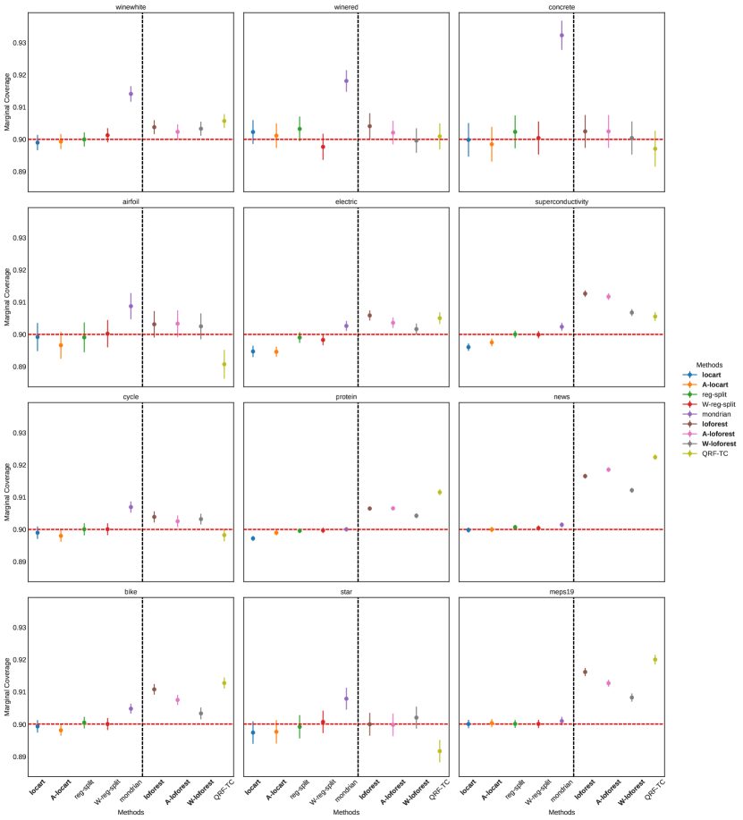
Figure 9: Marginal coverage 95% confidence interval of each method for each real dataset. The red dotted line indicates the nominal level ($1-\alpha=0.9$) and the black dotted line separates the conformal from the non-conformal methods. In general, all conformal methods are close to the nominal level for each real dataset, while the non-conformal ones present slight over-coverage in some of the datasets.

Regarding the marginal coverage of each method, Figure 9 in C reveals two main observations:

• Except for the Mondrian method, all conformal methods demonstrate marginal coverage that is close to the nominal level across all datasets. However, the Mondrian method exhibits over-coverage in small datasets such as winewhite, winered, concrete, and airfoil. This can be attributed to the large number of fixed bins ($k=30$) relative to the small sample sizes, resulting in bins with only a few instances grouped together. Consequently, larger cutoffs are generated in each partition.

• Among the non-conformal methods, some show slight over-coverage in specific datasets such as superconductivity, news, meps19, and bike. Notably, QRF-TC demonstrates occasional instances of under-coverage, as observed in the airfoil and star datasets. Thus, even though some of our methods are non-conformal, they generally exhibit marginal coverage at least greater than the nominal level.

Table 3: SMIS values for each method and real-world dataset. The average across 100 runs is reported with two times the standard deviation in brackets. Values in bold indicate the method with better performance in a 95% confidence interval. Both A-Locart and A-Loforest have good performance.

Type of method Dataset Conformal Non-conformal Locart A-Locart RegSplit W-RegSplit Mondrian Loforest A-Loforest W-Loforest QRF-TC Concrete 27.301 (0.526) 26.196 (0.497) 27.729 (0.542) 28.290 (0.442) 28.490 (0.399) 27.729 (0.542) 27.729 (0.542) 28.290 (0.442) 25.497 (0.487) Airfoil 10.395 (0.170) 10.232 (0.168) 10.915 (0.194) 10.140 (0.176) 10.587 (0.157) 10.341 (0.173) 10.201 (0.167) 10.085 (0.176) 9.533 (0.153) Wine white 2.950 (0.0217) 2.884 (0.023) 2.977 (0.022) 3.012 (0.021) 2.864 (0.021) 2.905 (0.022) 2.853 (0.021) 2.996 (0.021) 2.843 (0.021) Star 973.786 (6.959) 973.614 (7.094) 972.470 (7.053) 1042.652 (7.450) 1007.822 (7.278) 970.550 (6.959) 970.513 (6.981) 1039.369 (7.387) 997.357 (8.134) Wine red 2.780 (0.033) 2.750 (0.0307) 2.798 (0.033) 2.874 (0.031) 2.843 (0.031) 2.758 (0.032) 2.725 (0.031) 2.869 (0.030) 2.725 (0.034) Cycle 15.850 (0.118) 15.211 (0.120) 15.930 (0.121) 15.480 (0.110) 15.191 (0.115) 15.623 (0.116) 15.087 (0.118) 15.386 (0.109) 15.420 (0.109) Electric $\times\,\,(10^{-2})$ 5.360 (0.03) 5.320 (0.03) 5.580 (0.03) 5.050 (0.02) 5.340 (0.03) 5.220 (0.02) 5.190 (0.02) 4.990 (0.02) 5.170 (0.02) Bike 179.017 (1.549) 162.536 (1.112) 221.847 (1.832) 165.679 (1.098) 163.245 (1.126) 178.467 (1.397) 160.772 (1.105) 164.572 (1.074) 171.750 (1.242) Meps19 73.316 (0.977) 67.089 (1.068) 105.539 (1.191) 66.575 (1.033) 66.697 (1.105) 71.681 (0.957) 66.585 (1.068) 66.574 (1.005) 69.372 (0.966) Superconductivity 41.248 (0.280) 37.590 (0.223) 53.095 (0.283) 41.005 (0.230) 39.165 (0.223) 39.953 (0.237) 36.571 (0.212) 40.147 (0.225) 37.352 (0.214) News $\times\,(10^{4})$ 3.304 (0.043) 2.988 (0.040) 3.571 (0.043) 2.953 (0.040) 2.961 (0.042) 3.163 (0.041) 2.911 (0.040) 2.966 (0.040) 3.124 (0.040) Protein 16.607 (0.047) 14.039 (0.048) 17.583 (0.036) 14.693 (0.044) 14.045 (0.043) 16.303 (0.037) 13.812 (0.046) 14.612 (0.043) 15.388 (0.038)

Based on Table 3 and Figure 6, we also conclude the following:

• Table 3 demonstrates that our conformal and non-conformal methods, particularly A-Loforest and A-Locart, exhibit strong performance across most datasets, except for the airfoil dataset. Notably, A-Loforest shows remarkable performance in larger datasets such as protein, superconductivity, and bike-sharing data. This indicates that our adaptive partitioning of the feature space effectively functions in larger data and achieves favorable conditional coverage in such settings.

• Analyzing the first panel of Figure 6, we observe that our conformal proposal outperforms competing conformal methods in five datasets. Moreover, by referring to Table 3, we find that A-Locart generally performs equally or better than Mondrian, suggesting that our approach enhances the conditional variance binning of Mondrian by incorporating other features and increasing their flexibility.

• Further examination of Table 3 reveals that QRF-TC achieves superior performance in small datasets, notably the airfoil dataset, but lags behind other non-conformal and conformal methods in all other scenarios.

• Notably, for the star dataset, as indicated in Table 3, the regression split combined with our set of methods (Locart, A-Locart, Loforest, A-Loforest) outperforms other approaches.

• Overall, Figure 6 demonstrates that our class of methods achieves strong conditional coverage performance across real-world datasets.

Figure 6: Frequency of times each method performs better in real datasets according to SMIS in three different comparisons: between only conformal methods (first panel), between only non-conformal methods (second panel), and between all methods altogether (third panel). All panels suggest that both A-Locart and A-Loforest stand out as the most frequent methods. The third panel suggests also that, among all methods, A-Loforest has a superior performance across several real datasets.

Regarding the computational cost analysis of each method, Figure 7 exhibits a behavior similar to what was observed in the simulated experiments, but with some variations. In addition to Locart, A-Locart, and Mondrian, regression split is also identified as one of the most computationally efficient methods, with a running time spanning from 0.1% to close to 1% of the total analysis running time. Although the remaining methods, except for QRF-TC, demonstrate moderate to low computational costs (time consumption between 1% and 10%) for the majority of datasets, W-reg-split and W-Loforest exceed 10% consumption in the superconductivity and news datasets. This may be attributed to the high computational cost of training the MAD model in these contexts, which is avoided by both Loforest and A-Loforest.

Finally, we reinforce that QRF-TC is considerably more computationally costly than all the other methods in real data settings. For comparison, QRF-TC takes on average 14.4 seconds and 5 minutes to run concrete and protein datasets, respectively, while W-Loforest (the second most computationally heavy algorithm) takes 0.4 and 23 seconds to run each.

Figure 7: Mean proportion of running time spent in each method for each real dataset. Our methods are highlighted in bold. Even for medium to big data, our methods are still scalable compared to the remaining approaches.

5 Final Remarks

We propose two methods to calibrate prediction intervals: Locart and Loforest. These methods produce adaptive prediction intervals based on a sensible partition of the feature space created by training regression trees on conformity scores. A central aspect of Locart and Loforest is their applicability to high-dimensional settings, as our partition is not based on distance metrics on the feature space. Instead, this partition is obtained by grouping instances according to the conditional distribution of the conformal scores. Furthermore, these methods can be extended to calibrate prediction intervals based on any conformal score.

From a theoretical perspective, we show that Locart produces prediction intervals with marginal and local coverage guarantees. In addition, we prove that, under additional assumptions, Locart has asymptotic conditional coverage. Since Loforest is essentially an ensemble of Locart instances, we expect that Loforest inherits the properties of Locart while stabilizing the cutoff estimates that define the prediction intervals.

We validated our methods in simulated and real datasets, where they exhibited superior performance compared to baselines. In the simulated settings, our methods and their extensions, such as A-Locart and A-Loforest, present good conditional coverage and control the marginal coverage at the nominal level. The same holds when applying these methods to real data for both small and large samples. In all scenarios, our methods outperform established state-of-art algorithms, such as LCP and QRF-TC, including in running time comparisons.

We provide a Python package, named clover, that implements our methods using the scikit-learn interface and replicates all experiments done in this work. For future work, we intend to apply our class of methods to other conformal scores, thus improving their local coverage properties.

6 Acknowledgments

L. M. C. C. is grateful for the fellowship provided by Fundação de Amparo à Pesquisa do Estado de São Paulo (FAPESP), grant 2022/08579-7. R. I. is grateful for the financial support of FAPESP (grants 2019/11321-9 and 2023/07068-1) and CNPq (grant 309607/2020-5). M. P. O. was supported through grant 2021/02178-8, São Paulo Research Foundation (FAPESP). R. B. S. produced this work as part of the activities of FAPESP Research, Innovation and Dissemination Center for Neuromathematics (grant 2013/07699-0). The authors are also grateful for the suggestions given by Rodrigo F. L. Lassance.

Appendix A Failures of baselines

We recall, from the discussion of Section 3.1, that the oracle prediction interval depends on the conditional quantiles of the regression residual (calculated with the true regression function). Unless the data is homoscedastic, the residual is non-constant across the feature space, and so is its quantile when seen as a function of $\mathbf{x}\in{\mathcal{X}}$. Therefore, any method that seeks to approximate the oracle prediction interval (and inherit its optimal properties) should be based on conformity scores that adapt to the data’s local features. In the following, we present some data-generating processes where purportedly adaptive methodologies fail.

A.1 Locally weighted regression split

Let $\hat{\mu}$ be an estimator of the regression function. Lei et al. uses the conditional mean absolute deviation (MAD) of $[Y-\hat{\mu}(X)]|X=x$ to normalize prediction intervals. To see why this might fail, consider

$$Y|X=x\sim\begin{cases}\textrm{Laplace}(0,M),&\quad x\in[0,1),\\ \textrm{Beta}(\alpha,\beta),&\quad x\in[1,2],\end{cases}$$

where $\alpha=2,\beta=2$, and $M=\frac{2\alpha^{\alpha}\beta^{\beta}}{B(\alpha,\beta)(\alpha+\beta)^{\alpha+\beta+1}}$, with $B(\alpha,\beta)$ the Beta function. The conditional mean absolute deviation of $Y|X=x$ is constant and equal to $M$. The conditional quantiles of $|Y-\mu(X)|$, however, depend on whether $x\in[0,1)$ or $x\in[1,2]$. Therefore, normalizing with the MAD does not render the locally weighted regression residual adaptive in this situation.

Difficulty as conditional variance of $Y$

Boström et al. uses the empirical variance of predictions made by the trees of a Random Forest to normalize prediction regions. Even in the hypothetical scenario where we replace the empirical variance with the true conditional variance of the labels, $\mathbb{V}(Y|X=x)$, the variance-normalized prediction intervals cannot yield asymptotically valid prediction intervals. To see this, consider the mixture model

$$Y|X=x\sim 0.5\,N(-x,s^{2}-x^{2})+0.5\,N(x,s^{2}-x^{2}),$$

where we take $x\in[0,1]$ for simplicity and $s$ sufficiently large so as to $Y|X$ be unimodal. It is easy to show that $\mathbb{V}(Y|X=x)=s^{2}$, thus independent of $x$. On the other hand, the conditional quantiles of $|Y-\mu(X)|$ or of $|Y||X=x$ (since $\mu(x)=0$) depends on $x$: as $x$ increases, the density is concentrated at larger values of $x$, forcing the quantiles to drift away from zero. It follows that even if the samples have the same conditional variance – and thus, would be binned together in the approach of Boström et al. – they do not have the same distribution of regression residuals. Therefore, normalization with conditional variance cannot be used to construct prediction intervals that adapt to the data heteroscedasticity.

Appendix B Proofs

The proofs are organized into four subsections: B.1 proves that Locart has local and marginal validity (Theorem 2 and Corollaries 1 and 2), B.2 proves Theorem 3, B.3 proves the consistency of Locart (Theorem 4), and B.4 proves Locart asymptotic conditional validity (Theorem 5). Additionally, to conduct the proof on the last subsection (B.4) we make use of the following definitions:

Definition 2 (Convergence to the oracle prediction interval).

A prediction interval method $C(\cdot)$ converges to the oracle prediction interval $C^{*}(\cdot)$ if:

$$\mathbb{P}[Y_{n+1}\in C^{*}(\mathbf{X}_{n+1})\Delta C(\mathbf{X}_{n+1})]=o(1),\;\text{where $A\Delta B:=(A\cap B^{c})\cup(B\cap A^{c})$}\;.$$

Definition 3 (Asymptotic conditional validity (Lei et al., 2018)).

A prediction interval method $C(\cdot)$ satisfies asymptotic conditional validity if there exist random sets $\Lambda_{n}$, such that $\mathbb{P}[X_{n+1}\in\Lambda_{n}|\Lambda_{n}]=1-o_{\mathbb{P}}(1)$ and:

$$\sup_{\mathbf{x}_{n+1}\in\Lambda_{n}}\left|\mathbb{P}[Y_{n+1}\in C(\mathbf{X}_{n+1})|\mathbf{X}_{n+1}=\mathbf{x}_{n+1}]-(1-\alpha)\right|=o(1)\;.$$

B.1 Theorem 2

Proof of Theorem 2.

Let $A_{j}\in{\mathcal{A}}$ be an arbitrary partition element. Consider $I_{j}=\{i\in I_{\textrm{cal}}:\mathbf{X}_{i}\in A_{j}\}$. Since the full data $\{(\mathbf{X}_{i},Y_{i})\}_{i\in I_{\textrm{cal}}\sqcup\{n+1\}}$ is exchangeable, the scores $\hat{s}_{i}$ for $i\in I_{j}\sqcup\{n+1\}$ are exchangeable conditional on $I_{j}$ and $\mathbf{X}_{n+1}\in A_{j}$. Therefore, by the definition of $s^{*}_{j}$,

$$\mathbb{P}[Y_{n+1}\in C_{\textrm{local}}(\mathbf{X}_{n+1})|\mathbf{X}_{n+1}\in A_{j},I_{j}] =\mathbb{P}[\hat{s}(\mathbf{X}_{n+1},Y_{n+1})\leq s^{*}_{j}|\mathbf{X}_{n+1}\in A_{j},I_{j}]$$

$$\geq 1-\alpha.$$

Because this holds for all $I_{j}$, the bound is true after marginalizing over $I_{j}$. Thus,

$$\mathbb{P}[Y_{n+1}\in C_{\textrm{local}}(\mathbf{X}_{n+1})|\mathbf{X}_{n+1}\in A_{j}]\geq 1-\alpha.$$ (12)

As this holds for an arbitrary element $A_{j}$, (12) is valid for all $j=1,\dots,K$. Corollary 1 is proved by applying Theorem 2 in the Locart partition and Corollary 2 follows from Lei and Wasserman.∎

B.2 Theorem 3

Proof of Theorem 3.

To prove item 1 notice that if $\mathbf{x}_{1},\mathbf{x}_{2}\in A$, then $\hat{s}(\mathbf{X},Y)|\mathbf{X}=\mathbf{x}_{1}\sim\hat{s}(\mathbf{X},Y)|\mathbf{X}=\mathbf{x}_{2}$, which by Definition 1 implies directly that $t_{1-\alpha}^{*}(\mathbf{x}_{1})=t_{1-\alpha}^{*}(\mathbf{x}_{2})$ for any $\alpha\in(0,1)$. To show item 2, assume that $\mathbf{x}_{1},\mathbf{x}_{2}\in J$, and then $t_{1-\alpha}^{*}(\mathbf{x}_{1})=t_{1-\alpha}^{*}(\mathbf{x}_{2})$ for every $\alpha\in(0,1)$. Conclude that $F_{\hat{s}(\mathbf{X},Y)|\mathbf{X}=\mathbf{x}_{1}}^{-1}(1-\alpha|\mathbf{x}_{1})=F_{\hat{s}(\mathbf{X},Y)|\mathbf{X}=\mathbf{x}_{2}}^{-1}(1-\alpha|\mathbf{x}_{2})$ for every $\alpha\in(0,1)$. Thus, from the monotonicity and continuity of $F_{{\hat{s}(\mathbf{X},Y)|\mathbf{X}=\mathbf{x}}}$, we obtain that $F_{{\hat{s}(\mathbf{X},Y)|\mathbf{X}=\mathbf{x}}_{1}}(r|\mathbf{x}_{1})=F_{{\hat{s}(\mathbf{X},Y)|\mathbf{X}=\mathbf{x}}_{2}}(r|\mathbf{x}_{2})$ for all $r\in\mathbb{R}$. It follows that $\hat{s}(\mathbf{X},Y)|\mathbf{X}=\mathbf{x}_{1}\sim\hat{s}(\mathbf{X},Y)|\mathbf{X}=\mathbf{x}_{2}$, and therefore $\mathbf{x}_{1},\mathbf{x}_{2}\in A$. ∎

B.3 Theorem 4

Proof of Theorem 4.

Under Assumptions 1 and 2, the theorem follows from Lemma 34 in Izbicki et al. (2022). ∎

B.4 Theorem 5

To prove Theorem 5 we use the following Lemmas 1 and 2 proved below:

Lemma 1.

If a prediction interval method $C(\cdot)$ converges to the oracle prediction interval $C^{*}(\cdot)$, then it satisfies asymptotic conditional coverage.

Proof of Lemma 1.

Since $\mathbb{P}[Y_{n+1}\in C^{*}(\mathbf{X}_{n+1})\Delta C(\mathbf{X}_{n+1})]=o(1)$, it follows from Markov’s inequality and the dominated convergence theorem that

$$\mathbb{P}[Y_{n+1}\in C^{*}(\mathbf{X}_{n+1})\Delta C(\mathbf{X}_{n+1})|\mathbf{X}_{n+1}]=o_{\mathbb{P}}(1)\;.$$

Therefore, there exists $\phi_{n}=o(1)$ such that, for

$$\Lambda_{n+1}^{c}=\{\mathbf{x}_{n+1}\in{\mathcal{X}}:\mathbb{P}[Y_{n+1}\in C^{*}(\mathbf{X}_{n+1})\Delta C(\mathbf{X}_{n+1})|\mathbf{X}_{n+1}=\mathbf{x}_{n+1}]>\phi_{n}\}\;,$$

one obtains $\mathbb{P}[\mathbf{X}_{n+1}\in\Lambda_{n+1}^{c}]=o(1)$. Conclude that $\mathbb{P}[\mathbf{X}_{n+1}\in\Lambda_{n+1}]=1-o(1)$ and that:

$$\sup_{\mathbf{x}_{n+1}\in\Lambda_{n}}\Big{|}\mathbb{P}[Y_{n+1}\in C(\mathbf{X}_{n+1})|\mathbf{X}_{n+1}=\mathbf{x}_{n+1}]-(1-\alpha)\Big{|}$$

$$\leq\sup_{\mathbf{x}_{n+1}\in\Lambda_{n}}\Big{|}\mathbb{P}[Y_{n+1}\in C^{*}(\mathbf{X}_{n+1})\Delta C(\mathbf{X}_{n+1})|\mathbf{X}_{n+1}=\mathbf{x}_{n+1}]\Big{|}\leq\phi_{n}=o(1).$$

∎

Lemma 2.

Let $C^{*}=(\hat{\mu}(\mathbf{X}_{n+1})-t^{*}_{1-\alpha}(\mathbf{X}_{n+1}),\hat{\mu}(\mathbf{X}_{n+1})+t^{*}_{1-\alpha}(\mathbf{X}_{n+1}))$ and $C_{\textup{{Locart}}{}}=(\hat{\mu}(\mathbf{X}_{n+1})-\hat{t}_{1-\alpha}(\mathbf{X}_{n+1}),\hat{\mu}(\mathbf{X}_{n+1})+\hat{t}_{1-\alpha}(\mathbf{X}_{n+1}))$, where $\hat{t}(.)$ is the Locart estimated cutoff for a fixed induced partition. Under Assumption 1:

$$\mathbb{P}[Y_{n+1}\in C^{*}\Delta C_{\textup{{Locart}}{}}|\mathbf{X}_{n+1}]=o_{\mathbb{P}}(1)\;.$$

Proof of Lemma 2.

Under Assumption 1, $|t_{1-\alpha}^{*}(\mathbf{X}_{n+1})-\hat{t}_{1-\alpha}(\mathbf{X}_{n+1})|=o_{\mathbb{P}}(1)$ by Theorem 4. Thus, there exists $\lambda_{n}=o(1)$ such that $\mathbb{P}[|t_{1-\alpha}^{*}(\mathbf{X}_{n+1})-\hat{t}_{1-\alpha}(\mathbf{X}_{n+1})|>\lambda_{n}]=o(1)$. Note that, $\{Y_{n+1}\in C^{*}\Delta C_{\textup{{Locart}}{}}\}\subseteq\{|t_{1-\alpha}^{*}(\mathbf{X}_{n+1})-\hat{t}_{1-\alpha}(\mathbf{X}_{n+1})|>\lambda_{n}\}$. Thus:

$$\mathbb{P}[Y_{n+1}\in C^{*}\Delta C_{\textup{{Locart}}{}}] \leq\mathbb{P}[|t_{1-\alpha}^{*}(\mathbf{X}_{n+1})-\hat{t}_{1-\alpha}(\mathbf{X}_{n+1})|>\lambda_{n}]$$

$$=o(1)\,.$$

Since $\mathbb{P}[Y_{n+1}\in C^{*}\Delta C_{\textup{{Locart}}{}}]=o(1)$ if follows from Markov’s inequality that $\mathbb{P}[Y_{n+1}\in C^{*}\Delta C_{\textup{{Locart}}{}}|\mathbf{X}_{n+1}]=o_{\mathbb{P}}(1)$. ∎

Now, we prove Theorem 5.

Proof of Theorem 5.

Follows directly from Lemmas 1 and 2. ∎

Appendix C Experiments additional figures and tables

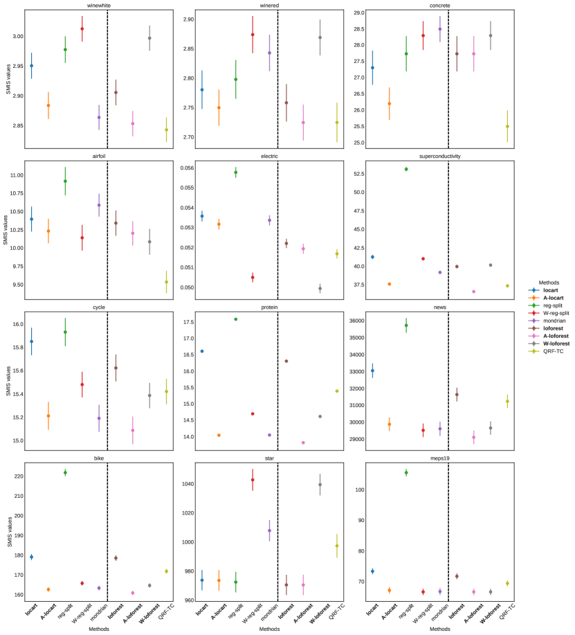
Figure 8: Smis 95% confidence interval of each method for each real dataset. The black dotted line separates the conformal from the non-conformal methods. We observe that A-Locart and A-Loforest stand out in several datasets and have good performances in general.

Table 4: Mean marginal coverage values of each method for each kind of simulation. The average across 100 simulations is reported with two times the standard error in brackets. Values in bold indicate methods with the most distant marginal coverage from the nominal ($1-\alpha=0.9$).

kind p Locart A-Locart RegSplit WRegSplit Mondrian Loforest A-Loforest W-Loforest QRF-TC Asym. 1 0.897 (0.001) 0.898 (0.001) 0.898 (0.001) 0.898 (0.001) 0.9 (0.001) 0.903 (0.001) 0.906 (0.001) 0.905 (0.001) 0.906 (0.001) Asym. 3 0.897 (0.001) 0.898 (0.001) 0.898 (0.001) 0.898 (0.001) 0.9 (0.001) 0.906 (0.001) 0.905 (0.001) 0.906 (0.001) 0.9 (0.002) Asym. 5 0.898 (0.001) 0.899 (0.001) 0.899 (0.001) 0.898 (0.001) 0.9 (0.001) 0.905 (0.001) 0.905 (0.001) 0.906 (0.001) 0.898 (0.002) Asym. 2 1 0.897 (0.001) 0.898 (0.001) 0.9 (0.001) 0.899 (0.001) 0.9 (0.001) 0.904 (0.001) 0.906 (0.001) 0.905 (0.001) 0.913 (0.001) Asym. 2 3 0.893 (0.001) 0.897 (0.001) 0.896 (0.001) 0.897 (0.001) 0.898 (0.001) 0.911 (0.001) 0.904 (0.001) 0.904 (0.001) 0.906 (0.001) Asym. 2 5 0.899 (0.001) 0.899 (0.001) 0.9 (0.001) 0.9 (0.001) 0.901 (0.001) 0.911 (0.001) 0.908 (0.001) 0.908 (0.001) 0.904 (0.001) Heterosc. 1 0.898 (0.001) 0.899 (0.001) 0.898 (0.001) 0.901 (0.001) 0.902 (0.001) 0.902 (0.001) 0.903 (0.001) 0.902 (0.001) 0.902 (0.001) Heterosc. 3 0.896 (0.001) 0.9 (0.001) 0.899 (0.001) 0.9 (0.001) 0.902 (0.001) 0.906 (0.001) 0.902 (0.001) 0.902 (0.001) 0.9 (0.001) Heterosc. 5 0.899 (0.001) 0.9 (0.001) 0.9 (0.001) 0.9 (0.001) 0.902 (0.001) 0.904 (0.001) 0.902 (0.001) 0.902 (0.001) 0.899 (0.002) Homosc. 1 0.9 (0.001) 0.9 (0.001) 0.9 (0.001) 0.901 (0.001) 0.902 (0.001) 0.901 (0.001) 0.901 (0.001) 0.902 (0.001) 0.897 (0.002) Homosc. 3 0.901 (0.001) 0.901 (0.001) 0.901 (0.001) 0.901 (0.001) 0.903 (0.001) 0.902 (0.001) 0.902 (0.001) 0.902 (0.001) 0.896 (0.002) Homosc. 5 0.901 (0.001) 0.901 (0.001) 0.901 (0.001) 0.901 (0.001) 0.902 (0.001) 0.902 (0.001) 0.901 (0.001) 0.903 (0.001) 0.895 (0.001) Non-corr. heterosc. 1 0.898 (0.001) 0.898 (0.001) 0.898 (0.001) 0.9 (0.001) 0.9 (0.001) 0.902 (0.001) 0.902 (0.001) 0.902 (0.001) 0.902 (0.001) Non-corr. heterosc. 3 0.896 (0.001) 0.897 (0.001) 0.899 (0.001) 0.9 (0.001) 0.901 (0.001) 0.906 (0.001) 0.904 (0.001) 0.902 (0.001) 0.9 (0.001) Non-corr. heterosc. 5 0.898 (0.001) 0.899 (0.001) 0.9 (0.001) 0.9 (0.001) 0.901 (0.001) 0.904 (0.001) 0.902 (0.001) 0.902 (0.001) 0.898 (0.002) $t$-residuals 1 0.9 (0.001) 0.9 (0.001) 0.9 (0.001) 0.901 (0.001) 0.902 (0.001) 0.903 (0.001) 0.904 (0.001) 0.904 (0.001) 0.897 (0.002) $t$-residuals 3 0.901 (0.001) 0.901 (0.001) 0.901 (0.001) 0.901 (0.001) 0.903 (0.001) 0.904 (0.001) 0.904 (0.001) 0.905 (0.001) 0.898 (0.002) $t$-residuals 5 0.901 (0.001) 0.901 (0.001) 0.901 (0.001) 0.902 (0.001) 0.903 (0.001) 0.904 (0.001) 0.904 (0.001) 0.906 (0.001) 0.898 (0.002)

References

- Butler and Rothman (1980) R. Butler, E. D. Rothman, Predictive intervals based on reuse of the sample, Journal of the American Statistical Association 75 (1980) 881–889.
- Neter et al. (1996) J. Neter, M. H. Kutner, C. J. Nachtsheim, W. Wasserman, et al., Applied linear statistical models (1996).
- Steinberger and Leeb (2016) L. Steinberger, H. Leeb, Leave-one-out prediction intervals in linear regression models with many variables, arXiv preprint arXiv:1602.05801 (2016).
- Papadopoulos et al. (2002) H. Papadopoulos, K. Proedrou, V. Vovk, A. Gammerman, Inductive confidence machines for regression, in: European Conference on Machine Learning, Springer, 2002, pp. 345–356.
- Vovk et al. (2005) V. Vovk, et al., Algorithmic learning in a random world, Springer Science & Business Media, 2005.
- Vovk et al. (2009) V. Vovk, I. Nouretdinov, A. Gammerman, et al., On-line predictive linear regression, The Annals of Statistics 37 (2009) 1566–1590.
- Lei et al. (2018) J. Lei, M. G’Sell, A. Rinaldo, R. J. Tibshirani, L. Wasserman, Distribution-free predictive inference for regression, Journal of the American Statistical Association 113 (2018) 1094–1111.
- Barocas et al. (2017) S. Barocas, M. Hardt, A. Narayanan, Fairness in machine learning, Nips tutorial 1 (2017) 2.
- Kleinberg et al. (2016) J. Kleinberg, S. Mullainathan, M. Raghavan, Inherent trade-offs in the fair determination of risk scores, arXiv preprint arXiv:1609.05807 (2016).
- Zhao et al. (2020) S. Zhao, T. Ma, S. Ermon, Individual calibration with randomized forecasting, in: International Conference on Machine Learning, PMLR, 2020, pp. 11387–11397.
- Lei and Wasserman (2014) J. Lei, L. Wasserman, Distribution-free prediction bands for non-parametric regression, Journal of the Royal Statistical Society: Series B (Statistical Methodology) 76 (2014) 71–96.
- Foygel Barber et al. (2021) R. Foygel Barber, E. J. Candes, A. Ramdas, R. J. Tibshirani, The limits of distribution-free conditional predictive inference, Information and Inference: A Journal of the IMA 10 (2021) 455–482.
- Romano et al. (2019) Y. Romano, E. Patterson, E. Candes, Conformalized quantile regression, in: H. Wallach, H. Larochelle, A. Beygelzimer, F. d'Alché-Buc, E. Fox, R. Garnett (Eds.), Advances in Neural Information Processing Systems, volume 32, Curran Associates, Inc., 2019. URL: https://proceedings.neurips.cc/paper_files/paper/2019/file/5103c3584b063c431bd1268e9b5e76fb-Paper.pdf.
- Izbicki et al. (2022) R. Izbicki, G. Shimizu, R. B. Stern, Cd-split and hpd-split: efficient conformal regions in high dimensions, Journal of Machine Learning Research (2022).
- Rasmussen and Williams (2005) C. E. Rasmussen, C. K. I. Williams, Gaussian Processes for Machine Learning, The MIT Press, 2005. doi:10.7551/mitpress/3206.001.0001.
- Koenker and Bassett (1978) R. Koenker, G. Bassett, Regression quantiles 46 (1978) 33–50. URL: https://www.jstor.org/stable/1913643. doi:10.2307/1913643.
- Koenker (2005) R. Koenker, Quantile Regression, Econometric Society Monographs, Cambridge University Press, 2005. doi:10.1017/CBO9780511754098.
- Meinshausen (2006) N. Meinshausen, Quantile regression forests, Journal of Machine Learning Research 7 (2006) 983–999.
- Efron and Gong (1983) B. Efron, G. Gong, A leisurely look at the bootstrap, the jackknife, and cross-validation, The American Statistician 37 (1983) 36–48. URL: https://www.jstor.org/stable/2685844. doi:10.2307/2685844.
- Breiman (1996) L. Breiman, Out-of-bag estimation, Technical Report, Statistics Department, University of California, 1996. URL: https://www.stat.berkeley.edu/users/breiman/OOBestimation.pdf.
- Neal (2012) R. Neal, Bayesian Learning for Neural Networks, Lecture Notes in Statistics, Springer New York, 2012. URL: https://books.google.com.br/books?id=LHHrBwAAQBAJ.
- Gal and Ghahramani (2016) Y. Gal, Z. Ghahramani, Dropout as a bayesian approximation: Representing model uncertainty in deep learning, in: M. F. Balcan, K. Q. Weinberger (Eds.), Proceedings of The 33rd International Conference on Machine Learning, volume 48 of Proceedings of Machine Learning Research, PMLR, New York, New York, USA, 2016, pp. 1050–1059. URL: https://proceedings.mlr.press/v48/gal16.html.
- Dey et al. (2022) B. Dey, D. Zhao, J. A. Newman, B. H. Andrews, R. Izbicki, A. B. Lee, Calibrated predictive distributions via diagnostics for conditional coverage, arXiv preprint arXiv:2205.14568 (2022).
- Dewolf et al. (2022) N. Dewolf, B. D. Baets, W. Waegeman, Valid prediction intervals for regression problems, Artificial Intelligence Review (2022) 1–37.
- Barber et al. (2021) R. F. Barber, E. J. Candès, A. Ramdas, R. J. Tibshirani, Predictive inference with the jackknife+ 49 (2021) 486–507. doi:10.1214/20-AOS1965.
- Papadopoulos et al. (2008) H. Papadopoulos, A. Gammerman, V. Vovk, Normalized nonconformity measures for regression conformal prediction, in: Proceedings of the IASTED International Conference on Artificial Intelligence and Applications (AIA 2008), 2008, pp. 64–69.
- Vovk (2012) V. Vovk, Conditional validity of inductive conformal predictors, in: Asian conference on machine learning, 2012, pp. 475–490.
- Valle et al. (2023) D. Valle, R. Izbicki, R. V. Leite, Quantifying uncertainty in land-use land-cover classification using conformal statistics, Remote Sensing of Environment 295 (2023) 113682.
- Chernozhukov et al. (2021) V. Chernozhukov, K. Wüthrich, Y. Zhu, Distributional conformal prediction, Proceedings of the National Academy of Sciences 118 (2021).
- Izbicki et al. (2020) R. Izbicki, G. Shimizu, R. B. Stern, Distribution-free conditional predictive bands using density estimators, in: Proceedings of AISTATS 2020, volume 108, 2020, pp. 3068–3077.
- Papadopoulos et al. (2011) H. Papadopoulos, V. Vovk, A. Gammerman, Regression conformal prediction with nearest neighbours, Journal of Artificial Intelligence Research 40 (2011) 815–840.
- Johansson et al. (2014) U. Johansson, H. Boström, T. Löfström, H. Linusson, Regression conformal prediction with random forests, Machine Learning 97 (2014) 155–176. doi:10.1007/s10994-014-5453-0.
- Boström and Johansson (2020) H. Boström, U. Johansson, Mondrian conformal regressors, in: Conformal and Probabilistic Prediction and Applications, PMLR, 2020, pp. 114–133.
- Boström et al. (2021) H. Boström, U. Johansson, T. Löfström, Mondrian conformal predictive distributions, in: Conformal and Probabilistic Prediction and Applications, PMLR, 2021, pp. 24–38.
- Papadopoulos and Haralambous (2010) H. Papadopoulos, H. Haralambous, Neural networks regression inductive conformal predictor and its application to total electron content prediction, in: K. Diamantaras, W. Duch, L. S. Iliadis (Eds.), Artificial Neural Networks – ICANN 2010, Lecture Notes in Computer Science, Springer, Berlin, Heidelberg, 2010, pp. 32–41. doi:10.1007/978-3-642-15819-3_4.
- Boström et al. (2017) H. Boström, H. Linusson, T. Löfström, U. Johansson, Accelerating difficulty estimation for conformal regression forests, Annals of Mathematics and Artificial Intelligence 81 (2017) 125–144. URL: https://api.semanticscholar.org/CorpusID:26467763.
- Ding et al. (2023) T. Ding, A. N. Angelopoulos, S. Bates, M. I. Jordan, R. J. Tibshirani, Class-conditional conformal prediction with many classes, 2023. doi:10.48550/ARXIV.2306.09335. arXiv:2306.09335.
- Guan (2021) L. Guan, Localized conformal prediction: A generalized inference framework for conformal prediction, arXiv preprint arXiv:2106.08460 (2021).
- Amoukou and Brunel (2023) S. I. Amoukou, N. J. Brunel, Adaptive conformal prediction by reweighting nonconformity score, arXiv preprint arXiv:2303.12695 (2023).
- Lin and Jeon (2006) Y. Lin, Y. Jeon, Random forests and adaptive nearest neighbors, Journal of the American Statistical Association 101 (2006) 578–590.
- Romano et al. (2020) Y. Romano, M. Sesia, E. J. Candès, Classification with valid and adaptive coverage (2020). doi:10.48550/ARXIV.2006.02544. arXiv:2006.02544.
- Angelopoulos et al. (2020) A. N. Angelopoulos, S. Bates, M. Jordan, J. Malik, Uncertainty sets for image classifiers using conformal prediction, in: International Conference on Learning Representations, 2020.
- Bian and Barber (2023) M. Bian, R. F. Barber, Training-conditional coverage for distribution-free predictive inference, Electronic Journal of Statistics 17 (2023) 2044–2066. doi:10.1214/23-EJS2145.
- Breiman (1993) L. Breiman, Classification and regression trees, Chapman & Hall, 1993.
- Pedregosa et al. (2011) F. Pedregosa, G. Varoquaux, A. Gramfort, V. Michel, B. Thirion, O. Grisel, M. Blondel, P. Prettenhofer, R. Weiss, V. Dubourg, J. Vanderplas, A. Passos, D. Cournapeau, M. Brucher, M. Perrot, Édouard Duchesnay, Scikit-learn: Machine learning in python, Journal of Machine Learning Research 12 (2011) 2825–2830. URL: http://jmlr.org/papers/v12/pedregosa11a.html.
- Cevid et al. (2022) D. Cevid, L. Michel, J. Näf, P. Bühlmann, N. Meinshausen, Distributional random forests: Heterogeneity adjustment and multivariate distributional regression, Journal of Machine Learning Research 23 (2022) 1–79. URL: http://jmlr.org/papers/v23/21-0585.html.
- Hastie et al. (2009) T. Hastie, R. Tibshirani, J. H. Friedman, J. H. Friedman, The elements of statistical learning: data mining, inference, and prediction, volume 2, Springer, 2009.
- Rahimi and Recht (2007) A. Rahimi, B. Recht, Random features for large-scale kernel machines, Advances in neural information processing systems 20 (2007).
- Fradkin and Madigan (2003) D. Fradkin, D. Madigan, Experiments with random projections for machine learning, in: Proceedings of the ninth ACM SIGKDD international conference on Knowledge discovery and data mining, 2003, pp. 517–522.
- Linusson et al. (2021) H. Linusson, I. Samsten, Z. Zając, M. Villanueva, nonconformist: Python implementation of the conformal prediction framework., https://github.com/donlnz/nonconformist, 2021.
- Amoukou and Brunel (2023) S. I. Amoukou, N. J. Brunel, ACPI: Adaptive conformal prediction intervals, https://github.com/salimamoukou/ACPI, 2023.
- Gneiting and Raftery (2007) T. Gneiting, A. E. Raftery, Strictly proper scoring rules, prediction, and estimation, Journal of the American statistical Association 102 (2007) 359–378.