Dynamically Generated Decoherence-Free Subspaces and Subsystems on Superconducting Qubits
Abstract
Decoherence-free subspaces and subsystems (DFS) preserve quantum information by encoding it into symmetry-protected states unaffected by decoherence. An inherent DFS of a given experimental system may not exist; however, through the use of dynamical decoupling (DD), one can induce symmetries that support DFSs. Here, we provide the first experimental demonstration of DD-generated DFS logical qubits. Utilizing IBM Quantum superconducting processors, we investigate two and three-qubit DFS codes comprising up to six and seven noninteracting logical qubits, respectively. Through a combination of DD and error detection, we show that DFS logical qubits can achieve up to a 23% improvement in state preservation fidelity over physical qubits subject to DD alone. This constitutes a beyond-breakeven fidelity improvement for DFS-encoded qubits. Our results showcase the potential utility of DFS codes as a pathway toward enhanced computational accuracy via logical encoding on quantum processors.
I Introduction
Scalable quantum computation relies on the ability to perform high-fidelity quantum logic operations. The path toward such operations is challenging due to inherent system-environment interactions and systematic errors. Ultimately, both induce noise processes that degrade qubit coherence and gate accuracy. Therefore, addressing noise in quantum systems is paramount to attaining viable and reliable quantum computation.
Broadly, approaches designed to manage noise in quantum systems seek to suppress, correct, or avoid errors [1]. Error suppression approaches (e.g., dynamical decoupling (DD) [2, 3, 4]) rely on the application of appropriately modulated control fields [5] such as fast and strong pulses to effectively average out noise [6]. In contrast, quantum error correction (QEC) leverages logical encodings of a collection of physical qubits to actively detect and correct errors [7, 8, 9, 10]. As a passive alternative, decoherence-free subspaces (DFSs) and noiseless subsystems (NS) form a special class of quantum codes that provide error avoidance by exploiting symmetries in the system-environment interaction [11, 12, 13, 14, 15, 16]. The three approaches can be unified under a single, symmetry-based framework [17]. Error mitigation, the newest category of quantum error management, utilizes information from an ensemble of quantum experiments to reduce noise-biasing in expectation values [18]. While in principle, each class of protocols can be employed on its own, it has long been appreciated that practical quantum error management schemes are likely to necessitate multiple approaches working in concert [19, 20, 21, 22, 23, 24, 25, 26, 27] to achieve utility-scale quantum computation and, eventually, fault tolerance [28].
Despite the elusiveness of fault tolerance, utility-scale quantum computing may be on the horizon in part due to advancements in error management. Demonstrations on currently available noisy quantum processors have showcased the potential for classes of protocols to be executed independently and simultaneously. For example, confirmation of quantum error mitigation’s effectiveness has been shown for quantum algorithms, such as the variational quantum eigensolver [29, 30] and quantum dynamics simulations [31]. Relatedly, a quantum algorithmic scaling advantage enabled by error suppression via DD has recently been demonstrated in superconducting systems [32] building on longstanding experimental evidence of its utility [33, 34, 35, 36, 37, 38, 39, 40, 41, 42, 43, 44, 45, 46, 47]. Combining the two approaches has also been shown to be fruitful for enhancing quantum algorithm performance [31].
Noisy quantum devices have further led to proof-of-principle demonstrations of QEC [48, 49, 50, 51, 52, 53, 54, 55]. This has included instances of error detection utilized to protect variational quantum algorithms [56]. Furthermore, verification of the added benefits of DD has been observed. For example, it has been incorporated into error correcting codes to protect idle qubits during long syndrome measurement acquisition and reset periods [51, 52, 55, 57, 58]. Error mitigation, DD, and quantum error detection have all been combined in a recent demonstration of better-than-classical execution of Grover’s algorithm [59].
Despite early experimental instantiations [60, 61, 62, 63, 64, 65, 66], DFSs have yet to be examined as a scalable approach to error management in the current quantum computing era [67]. Their ability to circumvent measurement-based feedback gives them a potential advantage over their error-correcting counterparts. Furthermore, DFS codes can be readily integrated with error suppression to dynamically engineer the required symmetries of the code [21, 68, 69, 70, 71, 72, 73, 74, 75]. Given their relative economy of qubit- and control-resource requirements, the question arises: what role can DFSs play in practical error management schemes for near-term and future quantum processors?
We address this question specifically for error-protected quantum memory and idle gates. DFSs are employed in conjunction with DD and error detection procedures to preserve logical qubit states on the IBM Quantum Platform (IBMQP) superconducting qubit processors. Specially designed DD sequences are used to engineer an effective noise environment and enforce symmetry conditions conducive to DFSs and NSs composed of two and three physical qubits, respectively. We present evidence for the existence of dynamically-generated DFSs and demonstrate their ability to surpass the fidelity of physical qubits subject to DD alone. The scalability of DFSs is showcased through the simultaneous generation and preservation of multiple logical qubits, where logical qubit fidelity up to 23% better than those achieved by the physical qubit constituents is observed. Together, these results highlight the potential utility of DFSs when used in conjunction with error suppression and detection procedures to enhance logical error management on quantum processors.
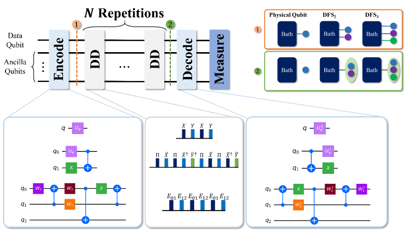
An overview of our methodology is presented in Fig. 1. Physical and logical protocols are compared by first encoding the qubits and then subjecting them to an error management protocol. As the objective is to evaluate each protocol’s ability to preserve qubit states, we apply repetitions of said protocols for equivalent time durations. State fidelity is then determined by applying a decoding operation and measuring in the computational basis. Physical qubits are protected by error suppression, while logical DFS qubits undergo error suppression and detection. We focus on the 2 and 3-qubit DFS code, with encoding operations and dynamical symmetry-generating sequences for each shown in the bottom-left and bottom-middle of Fig. 1, respectively. Error detection is applied after measurement via post-selection based on the state of the ancilla qubits.
This paper is organized as follows. In Section II, background on DFS codes and DD is presented. Sections III and IV showcase the results of the study. Evidence of collective interactions generated by logical DD is exhibited in Section III, while time-dependent preservation is the focus of Section IV. In the latter, we assess the performance of logical encodings against physical error suppression and highlight instances where DFS codes prevail. Section V summarizes the results and concludes.
II Decoherence-Free Subspaces and Dynamical Decoupling
II.1 Decoherence-Free Subspaces and Noiseless Subsystems
As passive error-correcting codes, DFSs leverage intrinsic symmetries in the system-environment interaction. Their construction is based on identifying subspaces of the system Hilbert space unaffected by noise. More concretely, consider an open quantum system described by the Hamiltonian
| (1) |
where is the pure system Hamiltonian and is the pure bath Hamiltonian, generating dynamics only within the system and bath Hilbert spaces and , respectively. The interaction between the system and its environment is captured by , which can be generically expressed as , where and act exclusively on the system and bath, respectively.
DFS encoding relies on finding a “good” subspace that is unaffected by . As long as the system is initialized in and no operations are performed by to take the system out of , the time evolution will be unaffected by the decoherence resulting from [15]. Group theoretic arguments show that under reasonable mathematical assumptions about the system operators , always exists and it is possible to perform scalable, universal quantum computation in the DFS [76]. More precisely, the system Hilbert space can be decomposed as a direct sum over the irreducible representations (irreps) of the associative algebra generated by the set : , such that each noiseless subsystem , where is the degeneracy of irrep , is invariant under the effects of [16]. That is,
| (2) |
where the states remain invariant under the error algebra , while can be altered by the arbitrary operator without consequence to the computation. Quantum information is stored in . When the irrep dimension , reduces to a DFS, i.e., a “good” subspace .
In this study, we employ DFS protection against collective interactions, which arises when the system-bath coupling is invariant under qubit permutation. The -qubit system-environment interaction under such permutation symmetry is fully described in terms of the total spin operator , where ; thus, . Below, DFS codes consisting of qubits will be denoted as DFSN for brevity.
II.1.1 Collective Dephasing DFS
The simplest type of collective system-bath interaction for which a DFS can be identified is collective dephasing, i,e., with . In turn, one can identify the smallest logical qubit encoded within two physical qubits. The subspace invariant under collective dephasing, which we refer to as DFS2, is spanned by the logical states and . A circuit describing the generation of an arbitrary state within the logical subspace is shown in Fig. 1. Logical manipulations that preserve the DFS consist of all Hermitian operators that belong to the commutant of the error algebra, , i.e., all operators that commute with the noise. One such set of encoding operators is given by
| (3a) | ||||
| (3b) | ||||
where [76, 77]. Logical rotations within the DFS are therefore defined by , where .
II.1.2 Collective Decoherence DFS
Decoherence-free subsystems, or NSs, build upon the notion of noise-invariant subspaces to more generally define subsystems corresponding to preserved degrees of freedom. Such a subsystem can be constructed when a quantum system is subject to collective decoherence, i.e., and , using a minimum of three physical qubits [16, 78]. The logical space is constructed from four orthonormal states:
| (4) | ||||
These states are composed of the singlet state and triplet states , , and . The 3-qubit code (DFS3) is defined by the logical states
| (5) | ||||
where and specify the gauge. Note that here the gauge degrees of freedom are that of a single qubit and thus, . Fig. 1 displays the encoding circuit for the DFS3 code with and ; see Appendix A for an extension to arbitrary and . Computations on the three-qubit code are generated by the logical operators [76]:
| (6) | ||||
| (7) |
where denotes a SWAP operation between the th and th physical qubits. We note as an aside, that this forms the basis for universal quantum computation using just the Heisenberg interaction [76, 79, 80], specifically in quantum dot systems [81, 75, 82].
II.2 Error Detection in DFS Codes
Passive quantum codes share many commonalities with their active correcting counterparts. Specifically, DFSs can be described as a highly degenerate quantum error correcting code with infinite distance when all operations are restricted to the code space. Of course, in practice, logical operations are not ideal and leakage outside of the code space can occur. It is in this domain that the stabilizer properties of the DFS codes can be employed for an additional layer of protection.
Under the stabilizer formalism, continuous (non-Abelian) stabilizers can be defined based on the DFS condition, Eq. 2 [76]. Collective dephasing yields as one of the stabilizer elements, while collective decoherence includes additional collective Pauli operations as stabilizer elements: and . As a result, the DFS can detect any odd number of single-qubit bit-flips under collective dephasing or of arbitrary single-qubit Pauli errors under collective decoherence. We utilize the error detection properties of the code here by performing post-selection (PS) after decoding. Measurement outcomes of data qubits are post-selected based on the state of specific ancilla qubits. Below, we show that the PS procedure boosts the code’s ability to maintain logical states.
II.3 Dynamically Generated DFSs
II.3.1 Dynamical Decoupling
Quantum processors rarely possess intrinsic noise environments with the ideal permutation symmetry of collective interactions. However, through the use of DD, such symmetries can be effectively engineered. DD sequences generally comprise control pulses applied at predetermined time intervals to modify the system-environment interaction . Given a unitary evolution subject to the total Hamiltonian [Eq. 1],
| (8) |
DD sequences with delta-function-like pulses result in the evolution
| (9) |
The total evolution time and are the control pulses. Conventionally, DD sequences are designed to effectively cancel the system-bath interaction (i.e., ) up to a certain order in . More precisely, an th order decoupling sequence yields an effective time evolution given by , where depends on both and [26, 83]. A notable example, which will be relevant in this study, is the universal decoupling sequence [3]
| (10) |
Utilizing and pulses, representing -rotations about the and axes of the single qubit Bloch sphere, respectively, offers first order () decoupling for general single qubit noise.
Beyond suppression of system-environment interactions, DD can be used to selectively average out components of to create the necessary conditions for a DFS. The group-theoretic foundations for such “symmetrizing” sequences are given in Refs. [4, 21]. Specific sequences for generating collective interactions are derived in Ref. [68] and are elaborated upon below. In principle, achieving symmetrization conditions conducive to a DFS can require fewer pulses than complete suppression of general multi-qubit system-environment interactions [84]; this is a potential advantage of combining DFSs with DD.
II.3.2 Dynamically Generated Collective Dephasing
Two-qubit collective dephasing is generated by DD sequences consisting of logical operations. In the most general two-qubit setting, where single and two-qubit couplings to the environment are allowed, two-qubit collective dephasing is created by a concatenation of three sequences consisting of rotations on the logical Bloch sphere (see Appendix B):
| (11) |
The inner-most sequence composed of operations is used to suppress leakage out of the DFS. In contrast, concatenating logical operators and enables cancellation of all logical single-qubit errors. Note that the suppression properties of the sequence are independent of concatenation ordering. All variations lead to an effective Hamiltonian with .
II.3.3 Dynamically Generated Collective Decoherence
The three-qubit collective decoherence condition can be generated using the sequence
| (12) |
Intuitively, the resulting evolution is akin to rapidly swapping the states of the qubits such that the environment cannot distinguish between them [75]. The sequence assumes the underlying noise model is given by , with and . The effective Hamiltonian resulting from the DD sequence is .
Practical implementation of the above sequences on the IBMQP requires composite pulses consisting of multiple noisy two-qubit gates. For example, includes three CNOTs, each of which demands two faulty cross-resonance gates [85]; see Appendix C for further details. As such, realizations of these sequences are quite far from the noiseless, delta-function-pulse idealization from which they were derived. Nonetheless, as we show below, dynamically generating DFSs with these composite operations is achievable despite the imperfections inherent in the two-qubit gates.
III Evidence of Collective Symmetry
III.1 Logical State Invariance
We investigate the presence of native and dynamically generated collective decoherence on the IBMQP. A single logical qubit is compared against its physical qubit constituents using a state-dependent fidelity analysis. The system is prepared in a quantum state lying in the -plane of the Bloch sphere, such that for physical qubits and equivalently is defined for DFS codes. For the DFS3 code [Eq. 5], we first focus on the particular gauge and for this comparison. An investigation of gauge dependence is presented below. We do not scan over the azimuthal angle as previous work has shown that the free evolution fidelity depends almost entirely on the elevation angle [42, 46] (see the discussion following Eq. (15) in Ref. [86] for an explanation of this effect).
Following physical or encoded state preparation, the system is allowed to freely evolve or is subjected to DD; the resulting state is denoted by . An inverse state preparation completes the evolution prior to measurement in the computational basis. This sequence of operations is used to evaluate a physical or logical protocol’s ability to preserve an initial state via the state fidelity
| (13) |
where ideally . We investigate this fidelity as a function of for both unprotected states undergoing free evolution and protected states. The term “protected” refers to both DD and logical DFS encodings, or their combination.
Unprotected states are obtained from idle (free) evolution, where the system is allowed to evolve according to its internal dynamics after state preparation. In order to equalize qubit resources between unprotected and encoded states, we report the best fidelity of three adjacent physical qubits. Unprotected states are compared against DFS encodings without DD (DFS2, DFS3) and with DD (DFS2+DD, DFS3+DD). All results, unless otherwise specified, include PS. We find that PS leads to an overall increase in fidelity for both logical encodings whether or not DD is employed. This is discussed further in Section IV.1, with additional details presented in Appendix G.
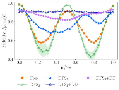
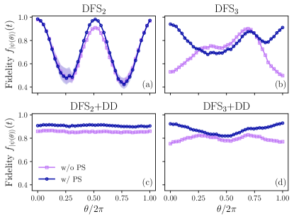
In Fig. 2, we show the state fidelity as a function of for a total evolution time of s, or one repetition of the DFS2+DD sequence, including logical state encoding/decoding. Experiments are performed on the five-qubit Manila device using qubits (2, 3, 4). While this subset of qubits yields the highest fidelity for logical encodings, we observe qualitatively similar behavior for alternative configurations; see Appendix H. Estimates of fidelity (solid lines) and 95% confidence intervals (CIs; shaded regions) are determined by bootstrapping over five realizations of the demonstration using measurement shots.

Logical encodings alone are not sufficient to observe collective dephasing/decoherence. The DFS2 code exhibits a state-dependent fidelity that is more consistent with free evolution. The DFS3 displays improved state fidelity, yet still a clear dependence upon the initial logical state. Thus, unsurprisingly, the IBMQP does not exhibit evidence of intrinsic collective interactions.
The inclusion of DD leads to substantially different behavior. The DFS2+DD protocol produces a near-state-invariant behavior consistent with collective dephasing. Similar results are observed for the DFS3+DD protocol, though some residual -dependence remains. Overall, DD substantially improves logical state fidelity and state invariance, consistent with dynamically generated collective interactions.
III.2 Gauge Invariance
Noiseless subsystems possess a gauge invariance that enables the logical computational basis states to be defined as subsystems, rather than subspaces. As an additional verification of collective decoherence generation, we examine the existence of this gauge invariance for the DFS3 code. We perform a state-dependent analysis similar to the previous subsection but also permit rotations within the gauge subspace. More concretely, we consider states of the form
| (14) |
where
| (15) | ||||
with the four constituent states defined in Eq. 4. The DFS3 code is prepared via the above state and subject to a single repetition of the DFS3+DD sequence or allowed to freely evolve for an equivalent duration. The state decoding procedure is performed before measurement in the computational basis and subsequent PS.
A comparison between a freely evolving DFS3 and the DFS3+DD protocol is shown in Fig. 3. Experiments are performed on the five-qubit Manila device using measurement shots. Estimates of mean fidelity [Eq. 13] are determined by bootstrapping over five realizations of the demonstration.
Evidence of gauge invariance is observed for both the DFS3 encoding alone and with the inclusion of the collective-symmetry-generating DD protocol. In the top panel of Fig. 3, the DFS3 fidelity determined via Eq. 13, is shown as a function of and . While there is a clear dependence of fidelity on the logical state, signatures of invariance to the gauge are more prominent. We quantify this invariance by examining the standard deviation of the fidelity over the gauge states and averaged over initial logical states. For the DFS3 encoding, the average standard deviation in fidelity is 0.023. In contrast, the DFS3+DD protocol exhibits an average standard deviation of 0.018. The absence of a significant difference in gauge invariance between the DFS3 and DFS3+DD protocols indicates that the gauge degree of freedom is robust under this device’s intrinsic decoherence mechanisms.
Consistent with the analysis in the previous subsection, DD improves the fidelity for all NS logical states. One of the most prominent features is the significant boost in fidelity for the gauge state with ; see the bottom panel of Fig. 3. This feature is easily explained by the state preparation circuit which requires an additional CNOT gate between the ancilla qubits for all . Ultimately, due to the topology of the hardware, this requires an additional SWAP operation as well; hence, the notable degradation in fidelity. Further details regarding the state preparation are discussed in Appendix A.
IV Preservation of Logical Qubits
Ultimately, the goal of our protection protocols is to extend the preservation of arbitrary quantum states. In this section, we evaluate each protocol’s performance by allowing the system to evolve under free or controlled evolution, i.e., the experiment depicted schematically in Fig. 1. Under unprotected (free) evolution, we prepare the state (we define below), let the system evolve according to its internal dynamics for fixed periods of time, apply , and measure in the computational basis. In the protected case, after encoding followed by the application of (logical-), the system is subject to repetitions of a DD sequence for a total evolution time of , where is the time for a single DD cycle. As in the case of free evolution, the experiment is completed by applying , decoding, and a measurement of all qubits in the computational basis. Below, we examine arbitrary state preservation for logical qubit encodings, starting with a single logical qubit and then scaling the protocols up to seven logical qubits. Unprotected states are compared against protected states using equivalent physical resources.
IV.1 Preservation of One Logical Qubit
First, we focus on the time-dependent state preservation of a single logical DFS qubit. Ideally, the preservation of an arbitrary state would be determined by sampling over the Haar distribution and calculating the average fidelity [87]. We estimate the Haar fidelity via
| (16) |
using an ensemble of states consisting of 14 Haar random states and the six eigenstates of the Pauli matrices, which we refer to as the poles of the Bloch sphere. We find this set to for estimating .
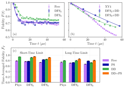
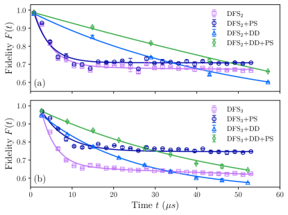
The average fidelity as a function of time is shown in Fig. 4 for experiments performed on the five-qubit Manila device. Mean fidelities and error bars are determined by bootstrapping over five realizations of the experiment and measurement shots. As in Section III.1, results are shown for the configuration of qubits with the highest average fidelity for logical encodings, i.e., qubits (2, 3, 4). Results for physical qubits consider the highest average fidelity among the three physical qubits used for the DFS3 code. While the DFS2 code only requires two physical qubits, we do not find a significant difference in performance when selecting the best performing qubit among two or three physical qubits. This holds for both the Free and XY4 cases. In the latter, the best performing qubit is typically the one subject to DD; hence, an additional neighbor qubit evolving freely does not alter the best performance.
Solid lines designate fits to the data using
| (17) | ||||
denote dimensionless weight parameters, such that
| (18) |
The time required to evolve the system for repetitions of a DD sequence (or the free evolution equivalent) is given by , where is the time for state encode, decode, and measurement. Short and long-term coherence times are determined by and , respectively, while is the oscillation frequency. Additional information regarding the fitting procedure can be found in Appendix F.
Figure 4(a) displays the time-dependent state-averaged fidelity for unprotected physical (Free) and logical (DFS2, DFS3) qubits subject to PS alone. The fidelities of the Free and DFS2 cases are statistically indistinguishable. However, the DFS3 case has a notably longer short-term decay time, while its long-time decay is essentially infinite; see Table 1. The longer decay time is accompanied by a higher fidelity. We attribute PS to the enhancement in fidelity, and substantiate this claim via an examination of the time-averaged fidelity:
| (19) |
In Figure 4(c), the time-averaged fidelity is shown for all protocols in two regimes designated by the DD repetition time of the sequence used for the DFS2 code. The short-time limit is set by the single repetition time , where , while the long-time limit corresponds to , i.e, . All estimates of are calculated by cubic spline integration, with subsequent means and CIs determined by bootstrapping.
The DFS3 code benefits substantially from PS in both the short and long-time limit. PS results in approximately 14% and 17% improvement in the DFS3 time-averaged fidelity over the bare encoding, respectively. The DFS2 code obtains a mere 1.3% and 3% in comparison. This result is consistent with the stabilizer properties of the code in the sense that the DFS2 code cannot detect all single-qubit errors and is limited to bit-flips. The DFS3 possesses a larger set of detectable errors and therefore, obtains a more robust code space.
| Protocol | (s) | (Hz) | (s) | |
|---|---|---|---|---|
| Free | 0 | |||
| XY4 | ||||
| DFS2 w/PS | 0 | |||
| DFS2 w/DD+PS | 0 | |||
| DFS3 w/PS | 0 | |||
| DFS3 w/DD+PS | 0 | 0.97 |
In examining the enhancement afforded by error detection as a function of the initial state, we find that the DFS3 particularly benefits from PS for states approaching the poles of the logical Bloch sphere; see Appendix G. States near the logical ()-plane suffer from logical errors that typically render lower fidelities with PS. In contrast, DFS2 logical states only gain from PS near the logical state. Ultimately, this behavior leads to state-averaged fidelities that favor DFS3 when error detection is employed.
Despite the utility of PS, DD typically results in greater improvement in fidelity. In the case of DFS2, the short-time decay rate is greatly enhanced by the inclusion of DD. For example, we observed an approximately 60% increase in when DD is used in conjunction with PS as compared to PS alone. Qualitatively similar behavior appears for the time-averaged fidelity as well. DD results in a short-time limit increase of 17% and long-time limit increase of 3% relative to PS. Further incorporating PS with DD boosts by 3% and 7%, respectively, indicating that (1) DD is most impactful in the short-time limit (consistent with DD’s propensity to suppress non-Markovian but not Markovian errors) and (2) both protocols perform best when used together.
The DFS3 code exhibits similar characteristics, however, PS plays an important role in the short-time limit as well. On their own, PS and DD enable similar short-time fidelities; DD yields a 15% increase over the DFS alone, with PS further improving the DFS3+DD fidelity by 7%. This is accompanied by a nearly 8 improvement in from s for DFS3 with PS to s when DD is incorporated. In contrast, DD has a less appreciable effect on in the long-time limit. DD enhances the time-averaged fidelity of the DFS3 code (without PS) by approximately 8%. DD and PS again prove to be more beneficial when used together, achieving a 21% increase over the DFS3 encoding alone.
In Fig. 4(b), the logical encoding schemes with PS and DD are compared against DD on physical qubits. Qubit 3 is subject to XY4, while qubits 2 and 4 are allowed to evolve freely. After each total evolution time, the best qubit fidelity is taken, where the DD cycle time is ns for a gate time of ns. Alternative physical DD protocols were considered as well, e.g., applying XY4 simultaneously on all qubits, however, they typically resulted in worse fidelity. We attribute the degradation in fidelity to quantum crosstalk, which is exacerbated by simultaneous operations on nearest-neighbor qubits. As such, the protocol chosen here is one such approach that suppresses parasitic interactions and combats local environmental noise.
Utilizing XY4 as a benchmark for noise protection in physical qubits, we evaluate each logical protocol’s ability to outperform its physical qubit constituents. We find that DFS2 (with DD and PS) and XY4 possess comparable short-time fidelity decay; see Table 1. Similar results are observed for the time-averaged fidelity in the short-time limit. However, in the long-time limit, the distinction between the protocols becomes more apparent. The DFS2 code with DD and PS achieves a 7.25% improvement over XY4, while the DFS3 code attains a 1.25% enhancement. Overall, these results indicate that it is possible for DFS encodings to perform on-par with physical error suppression protocols in the short-time limit, while providing greater long-term protection of quantum memory.
IV.2 Preservation of Multiple Logical Qubits
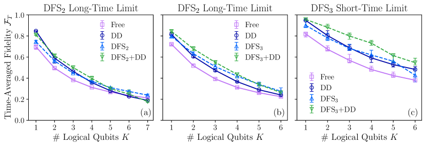
In order to justify the resource overhead of logical encoding, one must demonstrate that logical qubits can yield performance advantages over physical qubits, where is the encoding overhead, i.e., and for the DFS2 and DFS3 cases, respectively. The analysis in the previous subsection sheds light on this comparison for , where a single logical qubit performs similarly, if not better than physical qubits alone. We now expand this analysis to determine whether performance advantages persist with increasing . We focus on the preservation of the best physically adjacent logical (physical) qubits selected from a set of simultaneously generated logical (physical) qubits. The time-average fidelity serves as the comparison metric, where is the total time for encoding/decoding and one repetition of the DFS2+DD sequence, i.e., the so-called “short-time limit” discussed in Section IV.1.
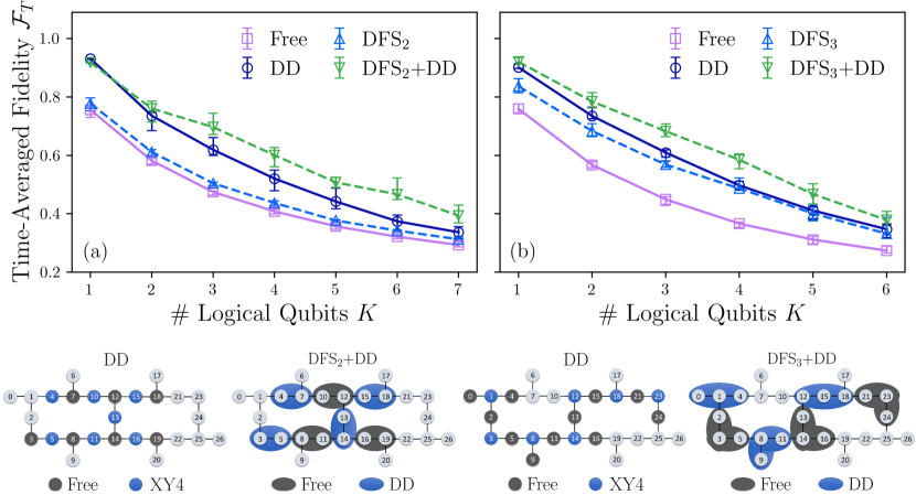
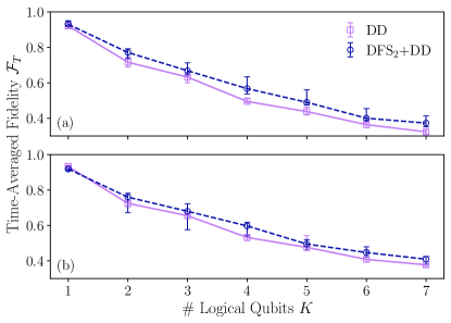
In Fig. 5, we summarize two comparisons in which () physical qubits are encoded into DFS2 ( DFS3) logical qubits on the 27-qubit Montreal device. The state-average fidelity is estimated for the states discussed in Section IV.1, using measurement shots. is determined by cubic spline integration of up to s. This is approximately equivalent to two repetitions of the DFS3 DD sequence, including state encode/decode procedures. Estimates of the mean and CI for the time-averaged fidelity are determined by bootstrapping.
Logical qubits are compared against physical qubits using a combination of DD and free evolution. We consider physical qubit protocols corresponding to free evolution on all qubits and a DD-protection scheme in which every other qubit within the array is subject to XY4. Those qubits not protected by DD are allowed to evolve freely. As in the case of the single logical qubit, this protocol outperforms simultaneously XY4 on all qubits due to its suppression of parasitic crosstalk [45, 47]. A schematic illustration of the DD protocol is shown below panels (a) and (b) in Fig. 5. We consider similar logical encoding schemes: (1) the qubits are prepared in the logical subspace and allowed to evolve freely and (2) upon preparing the logical subspaces, every other logical qubit is subject to the symmetrizing DD sequence. As in the case of the physical qubit DD-protection protocol, we find that simultaneous logical operations on neighboring qubits typically result in lower fidelity. As before, we suspect this behavior is due to crosstalk between neighboring physical qubits that propagates into logical errors. The logical qubit DD-protection protocols for the DFS2 and DFS3 encodings are summarized at the bottom of Fig. 5(a) and (b), respectively.
Above the protocol schematics in Fig. 5 are comparisons of the time-averaged fidelity as a function of the number of logical qubits for each protocol. In panel (a), results are shown for the DFS2 code. Among the available qubits, we select the best set of physically adjacent physical qubits based on CNOT gate error rates and decoherence times to perform our demonstrations. Physical qubit protocols are applied to the -qubit set, while the DFS2 protocols involve encoding the qubits into logical qubits. We then ask the question: requiring physical adjacency, how do the best logical qubits compare against the best physical qubits? Panel (a) summarizes our findings as a function of , where the DFS2 encoding with PS typically performs similarly to physical qubit free evolution. In contrast, upon incorporating DD, the DFS2 code outperforms the physical qubit DD protocol particularly for . Within error bars, the performance advantage of the DFS remains consistent up to , where time-averaged fidelities range from to higher than DD-protected physical qubits.
The performance advantage of DFS3 over physical qubits is even more substantial than DFS2. In Fig. 5(b), qubits are again selected based on CNOT gate error rates and decoherence times. Physical qubit protocols on qubits are compared against the DFS3 protocols on logical qubits. Contrary to the DFS3 code, the DFS3 code with PS alone yields sizable and consistent advantages over physical qubits subjected to free evolution; note the consistency with the discussion in Section IV.1. We find that this performance advantage persists as the number of logical qubits increases. Surprisingly, the benefits of the DFS3 with PS are considerable enough to result in near-equivalent time-averaged fidelity with that of DD on physical qubits, particularly for . As in the case of the DFS2 encoding, the inclusion of DD results in improved fidelity for the DFS3 code. The relative improvement in time-averaged fidelity varies from approximately to over the physical qubit DD protocol beyond . If instead the time-averaged fidelity is considered up to one cycle of the DFS3 (s) then a maximum improvement of over physical DD is achievable; a result comparable to the DFS2 case. In both cases, we find that DFS encoding, when combined with error detection and suppression outperforms physical error suppression on its own.
V Conclusions
In this work, we investigated the viability of DFS codes on currently available quantum devices. Using IBMQP superconducting qubit devices, we showed that DFS codes can achieve advantages over physical error suppression in the task of quantum state preservation. This was accomplished by devising logical qubit protection protocols that incorporate two key aspects: (1) noise-symmetrizing DD and (2) error detection provided by the stabilizer properties of the code. We established the advantage of these protocols for up to seven logical qubits, hence demonstrating their potential applicability and scalability on current and near-term quantum processors.
In evaluating the efficacy of the codes, we showed that the collective system-bath interactions required by DFS codes do not natively exist on the devices. However, such symmetries can be enforced through the application of specially designed pulse sequences. Despite their considerable gate depth, these sequences enable logical subspace invariance indicative of a DFS code with fidelity gains relative to unencoded qubits.
We showed that state invariance leads to improved logical qubit fidelity over error suppression protocols that are applied directly to physical qubits. We observed an enhancement in fidelity up to seven DFS2 and six DFS3 qubits encoded into and physical qubits, respectively. Error detection employed via post-selection resulted in logical qubit fidelities that surpass the XY4 DD sequence, particularly in the case of the DFS3 code. Moreover, when noise-symmetrizing DD was used in conjunction with post-selection, even greater performance gains were attainable. The DFS codes obtained up to a and improvement over XY4 in terms of the time-averaged fidelity, respectively. This constitutes a beyond-breakeven fidelity improvement for DFS-encoded qubits.
Additional studies are required to investigate the potential practical implementation of encoded quantum computation based on DFS codes. In particular, a demonstration of entangled logical qubits based on the methods we explored here is a natural next step. Nevertheless, we have already found encouraging results for the preservation of quantum states encoded within noninteracting copies of multiple logical qubits. Our protocol integrates error detection, avoidance, and suppression, and thus, highlights the significant potential of constructing error management schemes consisting of numerous techniques working in concert to enhance logical qubit fidelity.
VI Acknowledgements
GQ thanks Colin Trout for insightful discussions. BP is grateful to Dr. Namit Anand and Haimeng Zhang for useful comments. This work was supported in part by the U.S. Department of Energy (DOE), Office of Science, Office of Advanced Scientific Computing Research (ASCR) Quantum Computing Application Teams program under fieldwork proposal number ERKJ34 and the Accelerated Research in Quantum Computing program under Award Number DE-SC0020316. This research was supported by the ARO MURI grant W911NF-22-S-0007 and is based in part upon work supported by the National Science Foundation the Quantum Leap Big Idea under Grant No. OMA-1936388. This material is also based upon work supported by the Defense Advanced Research Projects Agency (DARPA) under Contract No. HR001122C0063. This research used resources of the Oak Ridge Leadership Computing Facility, which is a DOE Office of Science User Facility supported under Contract DE-AC05-00OR22725.
Appendix A DFS3 State Preparation
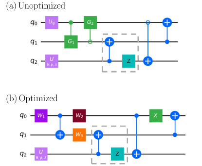
The DFS3 encoded states are prepared using the circuit defined in Ref. [88] and shown in Fig. 6. q0 denotes the data qubit, while q1 and q2 designate an additional ancilla qubit and gauge qubit, respectively. The controlled unitaries shown in the unoptimized circuit of Fig. 6(a) are defined via
| (22) | ||||
| (25) |
The circuit defined in the optimized circuit shown in Fig. 6(b) within the gray, dashed box is only executed if the gauge qubit is prepared in any state other than . Note that by definition of the DFS3 code, the gauge qubit can be initialized in any state while still satisfying the DFS preservation condition.
Compiling the state preparation circuit to the IBMQP gateset requires decomposition of the controlled gates and . The combined product of these gates can be replaced by a circuit that only requires one CNOT gate. This decomposition is accomplished via the Schmidt decomposition, where is rewritten as
| (26) |
where . The Schmidt decomposition is computed by taking the partial trace of each of the bipartite systems and computing the corresponding eigenvalues. For , we have and . We denote by the eigenvalues of . The eigenstates of and are and , respectively. The resulting unitaries from the decomposition are:
| (27) |
which can be derived from the Schmidt eigenvalues, and
The final optimized circuit is shown in Fig. 6(b).
Appendix B DFS2 DD Protocol
The DD sequence in Eq. 11 generates collective dephasing up to first-order in time-dependent perturbation theory. The sequence can achieve this suppression condition for general two-qubit system-environment interactions of the form
| (28) |
where denotes a bounded bath operator coupled to the system. The interaction Hamiltonian can be rewritten as
| (29) |
where denotes leakage errors, i.e., terms that cause transitions between states inside and outside of the DFS. The Hamiltonian includes operators that form undesirable logic gates on the DFS that couple to the bath and cause decoherence. Lastly, designates operators that either vanish or are proportional to identity on the DFS. The spanning subspaces for each Hamiltonian, in terms of the two-qubit Pauli basis are
| (30) |
where is the two-qubit identity operator and the logical operators in are defined in Eq. 3.
Following Ref. [70], it can be shown that logical operations can be used to design DD sequences that suppress all terms acting non-trivially on the DFS. Specifically, the sequence shown in Eq. 11 utilizes a concatenation of three sub-sequences that together suppress and in the ideal, instantaneous pulse limit. Each sub-sequence contains two pulses separated by free evolution periods of duration . As such, the generic construction of the sub-sequences can be defined by , where . Note that anticommutes with , so it suppresses leakage out of the DFS. The logical operators and can be used to suppress via a standard XY4 sequence, i.e., a concatenation of and . The concatenation of the leakage suppression and logical error suppression sequences yields the following sequence:
| (31) | ||||
where in the last line we used along with and .
Appendix C Implementation of DFS2 DD Pulses
The DD sequence used to generate the collective dephasing DFS the requires logical operations and . These logical unitaries are generated by logical operators and , respectively, which can take many forms. Belonging to the commutant of the error algebra only requires that the Hermitian operators be expressed as a linear combinations of the identity, , , and . The operators given in Eq. 3 define symmetric logical operators that satisfy the so-called independence property [76] (i.e., they act entirely within the specified DFS) and preserve all DFSs in the two-qubit Hilbert space [77]. Hence, operators on the logical subspace defined by do not enable mixing between the one-dimensional subspaces defined by and . While alternative, non-preserving logical operators, such as
| (32) | ||||
can be defined, empirical evidence shows that the symmetric operators yield higher fidelities.
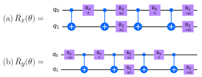
The preference towards the symmetric operators is quite surprising considering that their gate decomposition requires twice as many CNOT operators. This can be seen by utilizing commutativity to decompose the logical operators into products of two-local rotation operators. For example,
| (33) |
where each two-qubit interaction unitary can be decomposed into single qubit rotations bookended by CNOT gates; see Fig. 7(a). Following a similar decomposition, one obtains the circuit for in terms of the IBMQP gateset as shown in Fig. 7(b). The average logical gate time across the five data collection periods was s on the 5-qubit Manila device. The average logical gate time for the 27-qubit Montreal device was s.
Note that the definitions of non-symmetric logical operators yield unitaries similar to the first two-local interaction in the symmetric decomposition. For example, the non-symmetric logical -rotation operator is , which only requires two CNOT gates when decomposed via . Despite the reduction in gate time and depth, the non-symmetric operators do not outperform their symmetric counterparts.
Moreover, we do not observe improved performance from optimizing the gate decompositions of the symmetric logical operators. The decompositions given in Fig. 7 utilize four CNOTs, one more than what should be required for the decomposition of any two-qubit gate [87]. However, we find that optimizing the number of CNOT gates does not lead to better performance. We suspect that the four CNOT gate decomposition permits some form of inherent noise robustness not afforded by the optimized variation. Further investigation of the inherent hardware noise model is needed to fully understand this effect.
Appendix D DFS3 DD Protocol
The collective decoherence condition for the DFS3 code can be generated by the DD sequence shown in Eq. 12. This sequence is sufficient to symmetrize any linear system-environment interaction of the form
| (34) |
where and are bounded bath operators. In the ideal, instantaneous pulse limit, the dynamics after the sequence are governed by an effective Hamiltonian of the form , where is the duration of free evolution between pulses and . This result can be shown by writing the sequence as
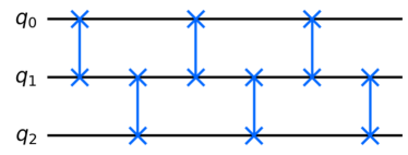
| (35) |
and computing the first-order term in the Magnus expansion with
| (36) |
Note that Eq. 35 can be reconciled with Eq. 12 by using and . The sequence’s circuit diagram is shown in Fig. 8.
Appendix E Hardware Specifications
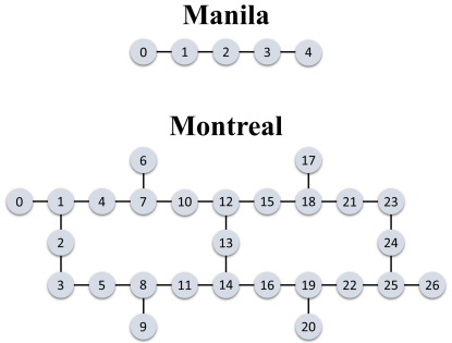
All demonstrations were performed on the IBMQP, a cloud-based quantum computing resource that offers access to superconducting transmon quantum processors. All circuits were written in Python using the Qiskit API created by IBM. We used the 5-qubit Manila and 27-qubit Montreal devices in our experiments. Each processor’s connectivity graph is shown in Fig. 9. The processor type, quantum volume (QV), and circuit layer operations per second (CLOPS) are detailed in Table 2.
| Device | Manila | Montreal |
|---|---|---|
| Processor | Falcon r5.11L | Falcon r4 |
| QV | 32 | 128 |
| CLOPS | 2.8K | 2.7K |
Qubit characteristics, such as , times, gate error rates, readout error rates, and gate durations for each device are presented in Tables 3-4. In all cases, qubit characteristics are collected over the duration of data collection, i.e., five realizations of each demonstration collected over multiple days. Values shown in the tables denote averages with error bars indicating one standard deviation.
Qubit characteristics for Manila are shown in Tables 3 and 4 for experiments performed during September 20-25, 2022. typically ranges from 120.8 s to 200 s, whereas varies from 43 s to 71.3 s. Single qubit gate error rates are on the order of and readout error rates on the order of . In Table 4, specifications for CNOT gate error rates and durations are shown to range from to and approximately 277 to 469 ns. Data is shown for control-target qubit pairs where the gate duration is shorter. Reverse ordering will incur an additional single qubit gate that increases both the error rate in accordance with Table 3 and gate duration by approximately 35.55 ns.
A similar set of data for Montreal is shown in Tables 5 and 6. We show data specifically for the qubits used in the demonstrations. Averages and standard deviations are determined from calibration data collected during October 11-20, 2022. Qubit relaxation and dephasing times vary across the device as s and s, respectively. Similar to Manila, single qubit gate error rates are on the order of and CNOT error rates are on the order of . Readout error rates are on the order of for a majority of the qubits used in the demonstrations. Variations in CNOT gate error rates are accompanied by varying duration for a significant subset of qubits; see Table 6.
| Qubit | 1Q Gate Error | Readout Error | ||
|---|---|---|---|---|
| 0 | ||||
| 1 | ||||
| 2 | ||||
| 3 | ||||
| 4 |
| Qubits (C,T) | CNOT Error Rate | CNOT Duration [ns] |
|---|---|---|
| (0,1) | 277.33 | |
| (1,2) | 469.33 | |
| (2,3) | 355.55 | |
| (4,3) | 298.67 |
| Qubit | 1Q Gate Error | Readout Error | ||
|---|---|---|---|---|
| 0 | ||||
| 1 | ||||
| 2 | ||||
| 3 | ||||
| 4 | ||||
| 5 | ||||
| 7 | ||||
| 8 | ||||
| 9 | ||||
| 10 | ||||
| 11 | ||||
| 12 | ||||
| 13 | ||||
| 14 | ||||
| 15 | ||||
| 16 | ||||
| 18 | ||||
| 19 | ||||
| 21 | ||||
| 23 | ||||
| 24 |
| Qubits (C,T) | CNOT Error Rate | CNOT Duration [ns] |
|---|---|---|
| (0,1) | ||
| (3,2) | ||
| (1,4) | ||
| (5,3) | ||
| (4,7) | ||
| (9,8) | ||
| (11,8) | ||
| (12,10) | ||
| (13,14) | ||
| (15,12) | ||
| (16,14) | ||
| (15,18) | 597.33 | |
| (16,19) | 270.22 | |
| (23,21) | 391.11 | |
| (23,24) |
Appendix F Data Collection and Analysis
F.1 Data Collection Practices
The IBMQP devices are subject to recalibration every few hours. During calibration, the characterization of qubit transition frequencies, error rates, and decoherence times are performed alongside updates to single-qubit and two-qubit pulse waveforms. We observe that qubit performance can vary significantly between, and even within, calibration cycles. Fluctuations in qubit characteristic parameters typically manifest as large shifts in fidelity when data is collected across calibrations. Furthermore, variations in the fidelity are observed depending upon when one performs the experiment. For example, experiments performed soon after a calibration can be distinct from those performed just before a calibration. While this variability is likely due to drift in qubit frequencies and/or the control master clock, knowledge of the potential origin of the errors does not necessarily imply that it is straightforward to mitigate.
Our demonstrations require a large suite of quantum circuits to be executed and thus, we are subject to data collection across multiple calibration cycles. In order to address the effects of hardware variability, we incorporate three practices in our circuit execution. Let us describe each practice by first defining a demonstration consisting of sets of circuits . Each set is composed of circuits each of approximately equivalent total time . For example, could describe a DD experiment where different DD repetitions are applied and consists of different DD sequences of equivalent total time.
The first practice is intrinsic to the definition of . During circuit creation, we organize the circuits such that those with the same total time are performed immediately after each other; hence, . In this manner, we aim to mitigate potential variability in the hardware noise environment as data is collected for different error protection protocols at the same . In addition, the order in which circuits are implemented is randomized with respect to . For example, a demonstration consisting of total times may be executed on hardware in the following order: . We find that this approach effectively averages variability due to calibrations across all rather than isolating it to specific total times. Lastly, multiple realizations (or replications) of each demonstration are executed over many hours or even days to collect data under a variety of hardware conditions. The data is then compiled and used to estimate various statistical quantities via bootstrapping. We find that this approach enables a more reliable estimate of an error protection protocol’s performance.
F.2 Bootstrapping
The results reported in the main text display the mean and confidence intervals estimated via the bootstrapping method described in Ref. [89]. This technique is implemented by randomly sampling data points (with replacement) from a data set of size and then computing the mean of this bootstrapped sample. By repeating this procedure times, a new, bootstrapped data set of size is generated. The mean and confidence interval (CI) can be calculated based on this bootstrapped data set. This approach is used to estimate mean fidelities and CIs for Eqs. 13, 16 and 19, which are used in the comparisons shown in Figs. 2-5.
F.3 Fitting Protocol
Data fits are performed for fidelity vs. time comparisons shown in Fig. 4. Bootstrapped estimates of fidelity are fit to the generic fit equation given in Eq. 17. Parameter reductions of the fit equation are also considered, most notably in cases where generic fits suggest parameters are inconsequential. Various fits derived from Eq. 17 are compared using the Akaike information criterion (AIC) [90], an estimator of prediction error. Fits shown in the main text correspond to the cases where AIC is minimal among the fit variations considered.
Appendix G Post-Selection Analysis
A crucial component for the success of the DFS codes is the use of post-selection (PS) to detect errors in the logical states. In the DFS2 protocol, post-selected states are aggregated based on the state of the ancilla qubit. Namely, combined two-qubit states in which the ancilla returns to the ground state after decoding are deemed viable. In the DFS3 code, the gauge qubit ( in Fig. 6) is used to identify valid states. In this section, we examine PS from a variety of different viewpoints to highlight its impact on fidelity and protocol resources.
G.1 State-Dependence
The impact of PS on fidelity is strongly dependent upon the logical state and encoding. In the case of the DFS2 code, only minor improvements in fidelity are found when using PS without error suppression. States near the state are particularly enhanced by PS, as can be seen in Fig. 10(a). Near equivalent fidelity between the DFS with and without PS suggests that the logical states are predominately plagued by logical errors or bit-flip errors rather than detectable single qubit phase-flip errors. Through DD, the logical fidelity greatly improves on average, and similarly, so does the effectiveness of error detection. The reduction of the logical error rate enables detectable errors to become more pronounced so that PS yields an average increase in the fidelity of 6.1%; see Fig. 10(c).
The DFS3 code offers a striking contrast to the DFS2 code when DD is not employed. States near the poles of the logical Bloch sphere are highly susceptible to noise that error detection can reduce considerably. This suggests that the primary error is of weight one. Conversely, states approaching the logical state are negatively impacted by PS, implying that logical errors are dominant. Despite these distinctions between the DFS2 and DFS3 codes, similarities re-emerge upon the introduction of DD. Symmetrization leads to an overall improvement in logical state fidelity and detectable errors. On average, PS yields a 9.7% improvement in the DFS3+DD fidelity. Illustrations of the DFS3 and DFS3+DD state dependence are shown in panels (b) and (d) of Fig. 10.

G.2 Time-Dependence
Investigating the effectiveness of PS as a function of time provides an alternative perspective on each protection protocol. In this section, we study the number of post-selected shots and state-averaged fidelity as a function of time. The former is shown in Fig. 11, while the latter is displayed in Fig. 12. Both are produced from the same data set used to create Fig. 4 in the main text; hence, they focus on the time-dependent state preservation of a single logical qubit.
The cost of PS is a reduction in the total number of experimental measurements (or shots) that can be used to estimate state fidelity. Fig. 11 illustrates the cost for each code with and without DD. Interestingly, DD does not always increase the total number of viable shots. In the case of the two-qubit protocol, the total number of post-selected shots reduces more slowly with the DFS alone. After one cycle of DD, the quantity of PS shots reduces by approximately 4%. Of course, this does not imply an increase in state fidelity due to the presence of logical errors, as is indicated by Fig. 4. DD with PS is still more advantageous than PS alone but ultimately requires more shots to achieve a particular sampling threshold.
The three-qubit DFS code contrasts with the two-qubit case. Specifically, the DFS3 code benefits from DD in regards to the total number of PS shots. The DFS3 code alone is subject to a dramatic reduction after approximately 10 s, where only about half of the total shots satisfy the PS criteria. DD affords a substantial improvement, increasing the total PS shot counts by over 31%. As such, PS and DD improve the total viable shot count and fidelity.
Despite the dissimilarity in total PS shot count between the codes, the trend in fidelity is universal: DD and PS used together typically supply the greatest positive impact on code performance. In Fig. 12, the state-averaged fidelity as a function of time is shown for each code under a variety of conditions. The data shown in each panel is used to produce the time-averaged fidelity shown in Fig. 4. It serves an additional purpose here, giving an additional viewpoint on PS and DD over a range of times not limited to the short- and long-time limits. This is particularly useful for observing crossovers in fidelity between protocols. For example, while DD+PS yields the highest fidelity for both protocols at short times (one repetition), PS is generally better suited for periods of long state preservation. The transition in preferred protocol arises due to apparent steady-state behavior in the fidelity that is inconsistent with the completely mixed state. In fact, it is more consistent with a convergence towards a partial symmetric subspace, most notably in the case of the DFS3 code. Further analysis is required to clarify this behavior.
| Configuration | Logical Qubits |
|---|---|
| 1 | (15,18),(10,12),(4,7),(13,14),(11,8),(16,19),(5,3) |
| 2 | (22,25),(20,19),(24,23),(21,18),(15,12),(13,14),(11,8) |
| 3 | (4,1),(2,3),(10,7),(5,8),(15,12),(11,14),(17,18) |
Appendix H Logical Qubit Fidelity and Qubit Variability
In the main text, we showcase demonstrations that provide evidence of logical encodings outperforming physical qubits via DFS codes combined with error detection and suppression. In Sections IV.1 and IV.2, data is shown for specific subsets of qubits on Manila and Montreal. In this section, we show that the behavior observed from these devices is not limited to those subsets; it can also be found in other qubit configurations.
H.1 One Logical Qubit
First, we focus on the single logical qubit case discussed in Section IV.1. The results shown in Fig. 4 are for the qubit mapping . While this subset of qubits yields the highest fidelity for the logical protection protocols, it is not the only subset that conveys an advantage from logical encoding. In Fig. 13, results are shown for two additional qubit configurations (a) and (b) ; see Fig. 9 for device topology. Average qubit fidelity is determined by bootstrapping over the set of 20 states discussed in Section IV.1. Mean fidelities and CIs are determined from one realization of the demonstration performed on October 20, 2022. Note that in both cases, the DFS encoding, DD, and PS together yield higher fidelities and slower fidelity decay rates than XY4 alone. Thus, empirical findings suggest that the relative improvements from the DFS protocol are robust to variability in qubit characteristics.
H.2 Multiple Logical Qubits
We further illustrate the robustness of the DFS code through additional studies of the time-averaged fidelity as a function of the number of logical qubits. In Fig. 14, the time-averaged fidelity in the short-time limit is shown for two additional configurations of physical qubits outlined in Table 7. Panel (a) and (b) display results for configurations 2 and 3, respectively, with configuration 1 shown in the main text (Fig. 5). Each panel contains a comparison between the physical DD and logical DFS2+DD (with PS) protocols outlined in Section IV.2. In both cases, the logical encoding performs similarly or somewhat better than physical-qubit DD, consistent with the results shown in the main text.
Appendix I Time-Averaged Fidelity at Different Integration Times
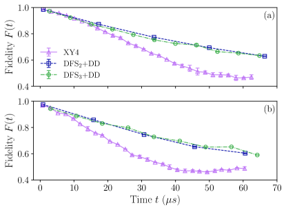
In the main text, results were shown for the time-averaged fidelity with an integration time equivalent to one DFS2+DD repetition, including encoding and decoding time. In this section, we consider additional integration times and examine the efficacy of each logical protocol. In Fig. 15, the DFS2 and DFS3 codes are compared against physical encoding schemes in the long-time limit in panels (a) and (b). Panel (c) compares the DFS3 code to physical encodings for an integration time of one DFS3+DD repetition with encoding and decoding. As in the main text, all logical protocols utilize PS.
Longer integration time lowers the fidelity. This is particularly true for both the physical DD and DFS2+DD protocols. Reduction in fidelity is accompanied by near equivalent performance among both DD-based protocols. Alternatively, the DFS2 without DD exhibits improvements in this regime such that it begins to outperform all protocols for . The steady-state behavior observed in Fig. 12 in the long-time limit ultimately explains this crossover in performance.
PS continues to be an essential part of the DFS3 protocol outperforming physical qubit error suppression. Both DFS3 and DFS3+DD achieve a higher fidelity than DD alone, with the advantage of the DFS3 increasing with . The performance improvement is so significant that both the DFS3 and DFS3+DD protocols perform nearly identically for .
Lastly, we comment on an additional short-time limit scenario relative to the DFS3 code. The main text defines the short-time limit as one cycle of the DFS2+DD sequence or approximately two cycles of the DFS3+DD sequence. Here, we consider an integration time of one DFS3+DD sequence, with results of this comparison shown in Fig. 15(c). The result is a more pronounced disparity between the physical and logical protocols. The DFS3 code achieves fidelities nearly equivalent to DD, while the DFS3+DD protocol yields a maximum improvement in of 23.6% over DD. The success of both protocols further justifies employing passive QEC codes as a viable logical encoding option for near-term devices.
References
- Lidar and Brun [2013] D. Lidar and T. Brun, eds., Quantum Error Correction (Cambridge University Press, Cambridge, UK, 2013).
- Viola and Lloyd [1998] L. Viola and S. Lloyd, Dynamical suppression of decoherence in two-state quantum systems, Phys. Rev. A 58, 2733 (1998).
- Viola et al. [1999] L. Viola, E. Knill, and S. Lloyd, Dynamical decoupling of open quantum systems, Physical Review Letters 82, 2417 (1999).
- Zanardi [1999] P. Zanardi, Symmetrizing evolutions, Physics Letters A 258, 77 (1999).
- Gordon et al. [2008] G. Gordon, G. Kurizki, and D. A. Lidar, Optimal dynamical decoherence control of a qubit, Phys. Rev. Lett. 101, 010403 (2008).
- Suter and Álvarez [2016] D. Suter and G. A. Álvarez, Colloquium: Protecting quantum information against environmental noise, Rev. Mod. Phys. 88, 041001 (2016).
- Shor [1995] P. W. Shor, Scheme for reducing decoherence in quantum computer memory, Physical review A 52, R2493 (1995).
- Steane [1996] A. M. Steane, Error correcting codes in quantum theory, Phys. Rev. Lett. 77, 793 (1996).
- Gottesman [1996] D. Gottesman, Class of quantum error-correcting codes saturating the quantum hamming bound, Phys. Rev. A 54, 1862 (1996).
- Gaitan [2008] F. Gaitan, Quantum Error Correction and Fault Tolerant Quantum Computing (Taylor & Francis Group, Boca Raton, 2008).
- Alicki [1988] R. Alicki, Limited thermalization for the Markov mean-field model of atoms in thermal field, Physica A: Statistical Mechanics and its Applications 150, 455 (1988).
- G.M. Palma, K.-A. Suominen and A.K. Ekert [1996] G.M. Palma, K.-A. Suominen and A.K. Ekert, Quantum Computers and Dissipation, Proc. R.. Soc. London Ser. A 452, 567 (1996).
- Zanardi and Rasetti [1997] P. Zanardi and M. Rasetti, Noiseless Quantum Codes, Physical Review Letters 79, 3306 (1997).
- Duan and Guo [1997] L.-M. Duan and G.-C. Guo, Preserving coherence in quantum computation by pairing quantum bits, Physical Review Letters 79, 1953 (1997).
- Lidar et al. [1998] D. A. Lidar, I. L. Chuang, and K. B. Whaley, Decoherence-free subspaces for quantum computation, Physical Review Letters 81, 2594 (1998).
- Knill et al. [2000] E. Knill, R. Laflamme, and L. Viola, Theory of quantum error correction for general noise, Phys. Rev. Lett. 84, 2525 (2000).
- Zanardi [2000] P. Zanardi, Stabilizing quantum information, Physical Review A 63, 012301 (2000).
- Cai et al. [2022] Z. Cai, R. Babbush, S. C. Benjamin, S. Endo, W. J. Huggins, Y. Li, J. R. McClean, and T. E. O’Brien, Quantum error mitigation, arXiv preprint arXiv:2210.00921 (2022).
- Lidar et al. [1999] D. A. Lidar, D. Bacon, and K. B. Whaley, Concatenating decoherence-free subspaces with quantum error correcting codes, Phys. Rev. Lett. 82, 4556 (1999).
- Lidar et al. [2000] D. A. Lidar, D. Bacon, J. Kempe, and K. Birgitta Whaley, Protecting quantum information encoded in decoherence-free states against exchange errors, Physical Review A 61, 052307 (2000).
- Viola et al. [2000] L. Viola, E. Knill, and S. Lloyd, Dynamical generation of noiseless quantum subsystems, Phys. Rev. Lett. 85, 3520 (2000).
- Alber et al. [2001] G. Alber, T. Beth, C. Charnes, A. Delgado, M. Grassl, and M. Mussinger, Stabilizing distinguishable qubits against spontaneous decay by detected-jump correcting quantum codes, Physical Review Letters 86, 4402 (2001).
- Alber et al. [2003] G. Alber, T. Beth, C. Charnes, A. Delgado, M. Grassl, and M. Mussinger, Detected-jump-error-correcting quantum codes, quantum error designs, and quantum computation, Physical Review A 68, 012316 (2003).
- Khodjasteh and Lidar [2002] K. Khodjasteh and D. A. Lidar, Universal fault-tolerant quantum computation in the presence of spontaneous emission and collective dephasing, Physical Review Letters 89, 197904 (2002).
- Khodjasteh and Lidar [2003] K. Khodjasteh and D. A. Lidar, Quantum computing in the presence of spontaneous emission by a combined dynamical decoupling and quantum-error-correction strategy, Physical Review A 68, 022322 (2003), erratum: ibid, Phys. Rev. A 72, 029905 (2005).
- Ng et al. [2011] H. K. Ng, D. A. Lidar, and J. Preskill, Combining dynamical decoupling with fault-tolerant quantum computation, Phys. Rev. A 84, 012305 (2011).
- Paz-Silva and Lidar [2013] G. A. Paz-Silva and D. A. Lidar, Optimally combining dynamical decoupling and quantum error correction, Sci. Rep. 3, 1530 (2013).
- Campbell et al. [2017] E. T. Campbell, B. M. Terhal, and C. Vuillot, Roads towards fault-tolerant universal quantum computation, Nature 549, 172 EP (2017).
- Dumitrescu et al. [2018] E. F. Dumitrescu, A. J. McCaskey, G. Hagen, G. R. Jansen, T. D. Morris, T. Papenbrock, R. C. Pooser, D. J. Dean, and P. Lougovski, Cloud quantum computing of an atomic nucleus, Phys. Rev. Lett. 120, 210501 (2018).
- Kandala et al. [2019] A. Kandala, K. Temme, A. D. Córcoles, A. Mezzacapo, J. M. Chow, and J. M. Gambetta, Error mitigation extends the computational reach of a noisy quantum processor, Nature 567, 491 (2019).
- Kim et al. [2023] Y. Kim, C. J. Wood, T. J. Yoder, S. T. Merkel, J. M. Gambetta, K. Temme, and A. Kandala, Scalable error mitigation for noisy quantum circuits produces competitive expectation values, Nature Physics , 1 (2023).
- Pokharel and Lidar [2023] B. Pokharel and D. A. Lidar, Demonstration of algorithmic quantum speedup, Physical Review Letters 130, 210602 (2023).
- Carr and Purcell [1954] H. Y. Carr and E. M. Purcell, Effects of diffusion on free precession in nuclear magnetic resonance experiments, Phys. Rev. 94, 630 (1954).
- Meiboom and Gill [1958] S. Meiboom and D. Gill, Modified spin-echo method for measuring nuclear relaxation times, Review of scientific instruments 29, 688 (1958).
- Haeberlen and Waugh [1968] U. Haeberlen and J. S. Waugh, Coherent averaging effects in magnetic resonance, Physical Review 175, 453 (1968).
- Biercuk et al. [2009a] M. J. Biercuk, H. Uys, A. P. VanDevender, N. Shiga, W. M. Itano, and J. J. Bollinger, Experimental uhrig dynamical decoupling using trapped ions, Physical Review A 79, 062324 (2009a).
- Biercuk et al. [2009b] M. J. Biercuk, H. Uys, A. P. VanDevender, N. Shiga, W. M. Itano, and J. J. Bollinger, Optimized dynamical decoupling in a model quantum memory, Nature 458, 996 (2009b).
- Sagi et al. [2010] Y. Sagi, I. Almog, and N. Davidson, Process tomography of dynamical decoupling in a dense cold atomic ensemble, Physical Review Letters 105, 053201 (2010).
- Naydenov et al. [2011] B. Naydenov, F. Dolde, L. T. Hall, C. Shin, H. Fedder, L. C. Hollenberg, F. Jelezko, and J. Wrachtrup, Dynamical decoupling of a single-electron spin at room temperature, Physical Review B 83, 081201 (2011).
- van der Sar et al. [2012] T. van der Sar, Z. H. Wang, M. S. Blok, H. Bernien, T. H. Taminiau, D. M. Toyli, D. A. Lidar, D. D. Awschalom, R. Hanson, and V. V. Dobrovitski, Decoherence-protected quantum gates for a hybrid solid-state spin register, Nature 484, 82 (2012).
- Souza et al. [2012] A. M. Souza, G. A. Álvarez, and D. Suter, Robust dynamical decoupling, Philosophical Transactions of the Royal Society A: Mathematical, Physical and Engineering Sciences 370, 4748 (2012).
- Pokharel et al. [2018] B. Pokharel, N. Anand, B. Fortman, and D. A. Lidar, Demonstration of Fidelity Improvement Using Dynamical Decoupling with Superconducting Qubits, Physical Review Letters 121, 10.1103/PhysRevLett.121.220502 (2018).
- Jurcevic et al. [2021] P. Jurcevic, A. Javadi-Abhari, L. S. Bishop, I. Lauer, D. F. Bogorin, M. Brink, L. Capelluto, O. Günlük, T. Itoko, N. Kanazawa, A. Kandala, G. A. Keefe, K. Krsulich, W. Landers, E. P. Lewandowski, D. T. McClure, G. Nannicini, A. Narasgond, H. M. Nayfeh, E. Pritchett, M. B. Rothwell, S. Srinivasan, N. Sundaresan, C. Wang, K. X. Wei, C. J. Wood, J.-B. Yau, E. J. Zhang, O. E. Dial, J. M. Chow, and J. M. Gambetta, Demonstration of quantum volume 64 on a superconducting quantum computing system, Quantum Sci. Technol. 6, 025020 (2021).
- Aharony et al. [2021] S. Aharony, N. Akerman, R. Ozeri, G. Perez, I. Savoray, and R. Shaniv, Constraining rapidly oscillating scalar dark matter using dynamic decoupling, Physical Review D 103, 075017 (2021).
- Tripathi et al. [2022] V. Tripathi, H. Chen, M. Khezri, K.-W. Yip, E. Levenson-Falk, and D. A. Lidar, Suppression of Crosstalk in Superconducting Qubits Using Dynamical Decoupling, Physical Review Applied 18, 024068 (2022).
- Ezzell et al. [2023] N. Ezzell, B. Pokharel, L. Tewala, G. Quiroz, and D. A. Lidar, Dynamical decoupling for superconducting qubits: A performance survey, Physical Review Applied 20, 064027 (2023).
- Zhou et al. [2023] Z. Zhou, R. Sitler, Y. Oda, K. Schultz, and G. Quiroz, Quantum crosstalk robust quantum control, Physical Review Letters 131, 210802 (2023).
- Boulant et al. [2005] N. Boulant, L. Viola, E. M. Fortunato, and D. G. Cory, Experimental implementation of a concatenated quantum error-correcting code, Phys. Rev. Lett. 94, 130501 (2005).
- Harper and Flammia [2019] R. Harper and S. T. Flammia, Fault-tolerant logical gates in the ibm quantum experience, Phys. Rev. Lett. 122, 080504 (2019).
- Andersen et al. [2020] C. K. Andersen, A. Remm, S. Lazar, S. Krinner, N. Lacroix, G. J. Norris, M. Gabureac, C. Eichler, and A. Wallraff, Repeated quantum error detection in a surface code, Nature Physics 16, 875 (2020).
- Chen et al. [2021] Z. Chen, K. J. Satzinger, J. Atalaya, A. N. Korotkov, A. Dunsworth, D. Sank, C. Quintana, M. McEwen, R. Barends, P. V. Klimov, et al., Exponential suppression of bit or phase errors with cyclic error correction, Nature 595, 383 (2021).
- Krinner et al. [2022] S. Krinner, N. Lacroix, A. Remm, A. Di Paolo, E. Genois, C. Leroux, C. Hellings, S. Lazar, F. Swiadek, J. Herrmann, et al., Realizing repeated quantum error correction in a distance-three surface code, Nature 605, 669 (2022).
- Sivak et al. [2023] V. Sivak, A. Eickbusch, B. Royer, S. Singh, I. Tsioutsios, S. Ganjam, A. Miano, B. Brock, A. Ding, L. Frunzio, et al., Real-time quantum error correction beyond break-even, Nature 616, 50 (2023).
- Miao et al. [2022] K. C. Miao, M. McEwen, J. Atalaya, D. Kafri, L. P. Pryadko, A. Bengtsson, A. Opremcak, K. J. Satzinger, Z. Chen, P. V. Klimov, et al., Overcoming leakage in scalable quantum error correction, arXiv preprint arXiv:2211.04728 (2022).
- Google Quantum AI [2023] Google Quantum AI, Suppressing quantum errors by scaling a surface code logical qubit, Nature 614, 676 (2023).
- Urbanek et al. [2020] M. Urbanek, B. Nachman, and W. A. de Jong, Error detection on quantum computers improving the accuracy of chemical calculations, Phys. Rev. A 102, 022427 (2020).
- Postler et al. [2023] L. Postler, F. Butt, I. Pogorelov, C. D. Marciniak, S. Heußen, R. Blatt, P. Schindler, M. Rispler, M. Müller, and T. Monz, Demonstration of fault-tolerant steane quantum error correction, arXiv preprint arXiv:2312.09745 (2023).
- Bluvstein et al. [2023] D. Bluvstein, S. J. Evered, A. A. Geim, S. H. Li, H. Zhou, T. Manovitz, S. Ebadi, M. Cain, M. Kalinowski, D. Hangleiter, et al., Logical quantum processor based on reconfigurable atom arrays, Nature , 1 (2023).
- Pokharel and Lidar [2022] B. Pokharel and D. Lidar, Better-than-classical Grover search via quantum error detection and suppression (2022), arXiv:2211.04543 [quant-ph] .
- Kwiat et al. [2000] P. G. Kwiat, A. J. Berglund, J. B. Altepeter, and A. G. White, Experimental verification of decoherence-free subspaces, Science 290, 498 (2000).
- Viola et al. [2001] L. Viola, E. M. Fortunato, M. A. Pravia, E. Knill, R. Laflamme, and D. G. Cory, Experimental realization of noiseless subsystems for quantum information processing, Science 293, 2059 (2001).
- Ollerenshaw et al. [2003] J. E. Ollerenshaw, D. A. Lidar, and L. E. Kay, Magnetic resonance realization of decoherence-free quantum computation, Phys. Rev. Lett. 91, 217904 (2003).
- Mohseni et al. [2003] M. Mohseni, J. S. Lundeen, K. J. Resch, and A. M. Steinberg, Experimental application of decoherence-free subspaces in an optical quantum-computing algorithm, Phys. Rev. Lett. 91, 187903 (2003).
- Fortunato et al. [2003] E. M. Fortunato, L. Viola, M. A. Pravia, E. Knill, R. Laflamme, T. F. Havel, and D. G. Cory, Exploring noiseless subsystems via nuclear magnetic resonance, Phys. Rev. A 67, 062303 (2003).
- Altepeter et al. [2004] J. B. Altepeter, P. G. Hadley, S. M. Wendelken, A. J. Berglund, and P. G. Kwiat, Experimental investigation of a two-qubit decoherence-free subspace, Phys. Rev. Lett. 92, 147901 (2004).
- Pushin et al. [2011] D. A. Pushin, M. G. Huber, M. Arif, and D. G. Cory, Experimental realization of decoherence-free subspace in neutron interferometry, Phys. Rev. Lett. 107, 150401 (2011).
- Preskill [2018] J. Preskill, Quantum Computing in the NISQ era and beyond, Quantum 2, 79 (2018).
- Wu and Lidar [2002] L. A. Wu and D. A. Lidar, Creating decoherence-free subspaces using strong and fast pulses, Phys. Rev. Lett. 88, 207902 (2002).
- Wu et al. [2002] L. A. Wu, M. S. Byrd, and D. A. Lidar, Efficient universal leakage elimination for physical and encoded qubits, Phys. Rev. Lett. 89, 127901 (2002).
- Byrd and Lidar [2002] M. S. Byrd and D. A. Lidar, Comprehensive encoding and decoupling solution to problems of decoherence and design in solid-state quantum computing, Phys. Rev. Lett. 89, 047901 (2002).
- Lidar and Wu [2003a] D. A. Lidar and L. A. Wu, Encoded recoupling and decoupling: An alternative to quantum error-correcting codes applied to trapped-ion quantum computation, Physical Review A 67, 032313 (2003a).
- Lidar and Wu [2003b] D. A. Lidar and L.-A. Wu, Quantum computers and decoherence: exorcising the demon from the machine, in Proc. SPIE, Noise and Information in Nanoelectronics, Sensors, and Standards, Vol. 5115 (2003) pp. 256–270.
- Byrd et al. [2005] M. S. Byrd, D. A. Lidar, L.-A. Wu, and P. Zanardi, Universal leakage elimination, Phys. Rev. A 71, 052301 (2005).
- Fong and Wandzura [2011] B. H. Fong and S. M. Wandzura, Universal quantum computation and leakage reduction in the 3-qubit decoherence free subsystem, Quantum. Inf. Comput. 11, 1003 (2011).
- West and Fong [2012] J. R. West and B. H. Fong, Exchange-only dynamical decoupling in the three-qubit decoherence free subsystem, New Journal of Physics 14, 083002 (2012).
- Kempe et al. [2001] J. Kempe, D. Bacon, D. A. Lidar, and K. B. Whaley, Theory of decoherence-free fault-tolerant universal quantum computation, Phys. Rev. A 63, 042307 (2001).
- Fortunato et al. [2002] E. M. Fortunato, L. Viola, J. Hodges, G. Teklemariam, and D. G. Cory, Implementation of universal control on a decoherence-free qubit, New Journal of Physics 4, 5 (2002).
- Yang and Gea-Banacloche [2001] C.-P. Yang and J. Gea-Banacloche, Three-qubit quantum error-correction scheme for collective decoherence, Physical Review A 63, 022311 (2001).
- D. Bacon, J. Kempe, D. P. DiVincenzo, D. A. Lidar, and K. B. Whaley [2001] D. Bacon, J. Kempe, D. P. DiVincenzo, D. A. Lidar, and K. B. Whaley, Encoded universality in physical implementations of a quantum computer, in Proceedings of the 1st International Conference on Experimental Implementations of Quantum Computation, Sydney, Australia, edited by R. Clark (Rinton, Princeton, NJ, 2001) p. 257, quant-ph/0102140 .
- J. Kempe, D. Bacon, D.P. DiVincenzo and K.B. Whaley [2001] J. Kempe, D. Bacon, D.P. DiVincenzo and K.B. Whaley, Encoded Universality from a Single Physical Interaction, Quant. Inf. Comput. 1, 33 (2001).
- DiVincenzo et al. [2000] D. P. DiVincenzo, D. Bacon, J. Kempe, G. Burkard, and K. B. Whaley, Universal quantum computation with the exchange interaction, Nature 408, 339 (2000).
- Weinstein et al. [2023] A. J. Weinstein, M. D. Reed, A. M. Jones, R. W. Andrews, D. Barnes, J. Z. Blumoff, L. E. Euliss, K. Eng, B. H. Fong, S. D. Ha, D. R. Hulbert, C. A. C. Jackson, M. Jura, T. E. Keating, J. Kerckhoff, A. A. Kiselev, J. Matten, G. Sabbir, A. Smith, J. Wright, M. T. Rakher, T. D. Ladd, and M. G. Borselli, Universal logic with encoded spin qubits in silicon, Nature 615, 817 (2023).
- Xia et al. [2011] Y. Xia, G. S. Uhrig, and D. A. Lidar, Rigorous performance bounds for quadratic and nested dynamical decoupling, Phys. Rev. A 84, 062332 (2011).
- Lidar [2014] D. A. Lidar, Review of decoherence-free subspaces, noiseless subsystems, and dynamical decoupling, in Quantum Information and Computation for Chemistry (John Wiley & Sons, Inc., 2014) pp. 295–354.
- McKay et al. [2018] D. C. McKay, T. Alexander, L. Bello, M. J. Biercuk, L. Bishop, J. Chen, J. M. Chow, A. D. Córcoles, D. Egger, S. Filipp, J. Gomez, M. Hush, A. Javadi-Abhari, D. Moreda, P. Nation, B. Paulovicks, E. Winston, C. J. Wood, J. Wootton, and J. M. Gambetta, Qiskit Backend Specifications for OpenQASM and OpenPulse Experiments, arXiv:1809.03452 [quant-ph] (2018), arXiv:1809.03452 [quant-ph] .
- Tripathi et al. [2023] V. Tripathi, H. Chen, E. Levenson-Falk, and D. A. Lidar, Modeling low- and high-frequency noise in transmon qubits with resource-efficient measurement (2023), arXiv:2303.00095 [quant-ph] .
- Nielsen and Chuang [2011] M. A. Nielsen and I. L. Chuang, Quantum Computation and Quantum Information: 10th Anniversary Edition, 10th ed. (Cambridge University Press, USA, 2011).
- Li et al. [2011] C.-K. Li, M. Nakahara, Y.-T. Poon, N.-S. Sze, and H. Tomita, Recursive encoding and decoding of the noiseless subsystem and decoherence-free subspace, Physical Review A 84, 044301 (2011).
- Stine [1989] R. Stine, An introduction to bootstrap methods: Examples and ideas, Sociological Methods & Research 18, 243 (1989).
- Stoica and Selen [2004] P. Stoica and Y. Selen, Model-order selection: a review of information criterion rules, IEEE Signal Processing Magazine 21, 36 (2004).