The Implicit Bias of Gradient Noise: A Symmetry Perspective

Abstract

We characterize the learning dynamics of stochastic gradient descent (SGD) when continuous symmetry exists in the loss function, where the divergence between SGD and gradient descent is dramatic. We show that depending on how the symmetry affects the learning dynamics, we can divide a family of symmetry into two classes. For one class of symmetry, SGD naturally converges to solutions that have a balanced and aligned gradient noise. For the other class of symmetry, SGD will almost always diverge. Then, we show that our result remains applicable and can help us understand the training dynamics even when the symmetry is not present in the loss function. Our main result is universal in the sense that it only depends on the existence of the symmetry and is independent of the details of the loss function. We demonstrate that the proposed theory offers an explanation of progressive sharpening and flattening and can be applied to common practical problems such as representation normalization, matrix factorization, and the use of warmup.

1 Introduction

Stochastic gradient descent (SGD) and its variants have become the cornerstone algorithms used in deep learning. In this work, we analyze the dynamics of SGD by working on its widely-adopted stochastic differential equation model (Li et al.,, 2019; Hu et al.,, 2017; Li et al., 2021a, ; Sirignano and Spiliopoulos,, 2020; Fontaine et al.,, 2021):

$$\mathop{}\!\mathrm{d}{\theta}_{t}=-\nabla L(\theta_{t})\mathop{}\!\mathrm{d}t+\sqrt{2\sigma^{2}\Sigma(\theta_{t})}\mathop{}\!\mathrm{d}W_{t},$$ (1)

where $\Sigma(\theta)$ is the covariance matrix of gradient noise (see Section 2 for details) with the prefactor $\sigma^{2}=\eta/(2S)$ modeling the impact of finite learning rate and batch size; $W_{t}$ denotes the Brownian motion. $\eta$ and $S$ denote the learning rate and batch size, respectively.

When $\sigma=0$, Eq. (1) corresponds to gradient descent (GD). However, SGD and GD can exhibit significantly different behaviors. A key observation is that SGD often converges to solutions that generalize better than those selected by GD in neural network training (Shirish Keskar et al.,, 2016; Wu et al.,, 2018; Zhu et al.,, 2018; Liu et al.,, 2021; Ziyin et al.,, 2022). Notably, even when $\sigma^{2}\ll 1$, suggesting a close resemblance between SGD and GD over finite time (Li et al.,, 2019), their long-time behaviors can still differ substantially (Pesme et al.,, 2021). These observations indicate that gradient noise can bias the dynamics significantly, and revealing the underlying mechanism is thus crucial for understanding the disparities between SGD and GD.

Contribution.

In this paper, we study the influence of SGD noise through a lens of symmetry. Our key contributions are summarized as follows. We show that

1. when symmetry exists in the loss function, the dynamics of SGD can be precisely characterized and is different from GD along the degenerate direction;

2. the treatment of common symmetries, including the rescaling and scaling symmetry in deep learning, can be unified in a single theoretical framework that we call the exponential symmetry;

3. every exponential symmetry has a unique and attractive fixed point along the degenerate direction for SGD;

4. important deep learning phenomena such as progressive sharpening/flattening and latent representation formation can happen as a result of symmetry and noise.

See Figure 1 for an illustration of our result for the simplest examples. We will apply the theory to various training settings in deep learning and show that the theory offers novel insights regarding various training techniques (such as minibatch training and warm-up) and components of common model architectures (such as normalization and matrix factorization). This work is organized as follows. We present the main theoretical results in Section 3. We apply our theory to understand specific problems and present numerical results in Section 4. We discuss the most closely related works in Section 5. The last section concludes this work and points to important future problems. All the proofs are presented in the Appendix.

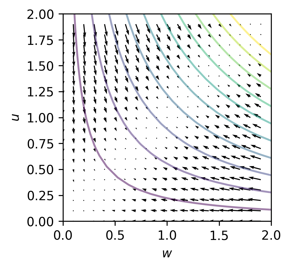
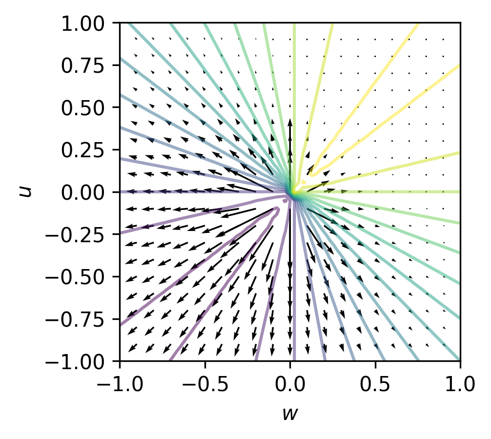
Figure 1: SGD has a systematic bias in the degenerate directions of the loss landscape. The solid lines show the equipotential lines of the loss, and the arrows show the projections of the parameter update in the degenerate directions. Let $x$ be a standard normal variable. Left: the loss function $\ell=uwx$ contains a rescaling symmetry. Right: $\ell=\frac{u+w}{\sqrt{u^{2}+w^{2}}}x$ contains a scaling symmetry. In both cases, the SGD has a nonvanishing flow along the degenerate directions of the loss. More importantly, the flows are monotonic and vanish at a unique and attractive point ($u=w$ for rescaling symmetry and $|u|$, $|w|=\infty$ for scaling symmetry) along each equipotential line. This behavior is qualitatively different from GD, where the motion along the degenerate direction vanishes.

2 Preliminaries

Setup and Notations.

Let $\ell:\Omega\times\mathcal{Z}\mapsto\mathbb{R}$ denote the per-sample loss, with $\Omega$ and $\mathcal{Z}$ denoting the parameter and sample space, respectively. Here, $z\in\mathcal{Z}$ includes both the input and label and accordingly. We use $\mathbb{E}_{z}=\mathbb{E}$ to denote the expectation over of a given training set. Therefore, $L(\theta)=\mathbb{E}_{z}[\ell(\theta,z)]$ is the empirical risk function. The covariance of gradient noise is given by

$$\Sigma(\theta)=\mathbb{E}_{z}[\nabla\ell(\theta,z)\nabla\ell(\theta,z)^{\top}]-\nabla L(\theta)\nabla L(\theta)^{\top}.$$

Additionally, we use $\Sigma_{v}(\theta):=\mathbb{E}_{z}[\nabla_{v}\ell(\theta,z)\nabla_{v}\ell(\theta,z)^{\top}]-\nabla_{v}L(\theta)\nabla_{v}L(\theta)^{\top}$ to denote the covariance of gradient noise impacting on the subset of parameters $v$. Denote by $(\theta_{t})_{t\geq 0}$ the trajectory of SGD or GD. For any $h:\Omega\mapsto\mathbb{R}$, we write $h_{t}=h(\theta_{t})$ and $\dot{h}(\theta_{t})=\frac{\mathop{}\!\mathrm{d}}{\mathop{}\!\mathrm{d}t}h(\theta_{t})$ for brevity. When the context is clear, we also use $\ell(\theta)$ to denote $\ell(\theta,z)$.

Symmetry.

The per-sample loss $\ell(\cdot,\cdot)$ is said to possess the $Q$-symmetry if

$$\ell(\theta,z)=\ell(Q_{\rho}(\theta),z),\forall\rho\in\mathbb{R},$$ (2)

where $(Q_{\rho})_{\rho\in\mathbb{R}}$ is a set of transformation parameterized by $\rho\in\mathbb{R}$. Without loss of generality, we assume $Q_{0}=\mathrm{id}$. The most common symmetries exist within the model $f$, namely $f_{\theta}$ is invariant under certain transformations of $\theta$. However, our formalism is slightly more general in the sense that it is also possible for the model to be variant while the per-sample loss remains unchanged, which appears in self-supervised learning (Ziyin et al., 2023b, ), for example.

3 General Theory

By taking the derivative with respect to $\rho$ at $\rho=0$ in Eq. (2), we have

$$0=\nabla_{\theta}\ell(\theta,z)\cdot J(\theta),$$ (3)

where $J(\theta)=\frac{\mathop{}\!\mathrm{d}Q_{\rho}(\theta)}{\mathop{}\!\mathrm{d}\rho}|_{\rho=0}$. Denote by $C$ be the antiderivative of $J$, that is, $\nabla C(\theta)=J(\theta)$. Then, taking the expectation over $z$ in (3) gives the following conservation law for GD solutions $(\theta_{t})_{t\geq 0}$:

$$\dot{C}(\theta_{t})=0.$$ (4)

Essentially, this is a consequence of the Noether’s theorem (Noether,, 1918), and $C$ can be called a “Noether charge.” The conservation law (4) implies that the GD trajectory is constrained on the manifold $\{\theta:C(\theta)=C(\theta_{0})\}$. We refer to Kunin et al., (2020) for a study of this type of conservation laws under the Bregman Lagrangian (Jordan,, 2018).

3.1 Noether Flow in Degenerate Directions

In this paper, we are interested in how $C(\theta_{t})$ changes, if it changes at all, under SGD. By Ito’s lemma, we have the following Noether flow:

$$\dot{C}(\theta_{t})=\sigma^{2}{\rm Tr}\left[\Sigma(\theta_{t})\nabla^{2}C(\theta_{t})\right],$$ (5)

where $\nabla^{2}C$ denotes the Hessian matrix of $C$. The derivation is deferred to Appendix A. By definition, $\Sigma(\theta_{t})$ is always positive semidefinite (PSD). Thus, we immediately have: if $\nabla^{2}C$ is PSD throughout training, $C(\theta_{t})$ is a monotonically increasing function of time. Conversely, if $\nabla^{2}_{\theta}C$ is negative semidefinite (NPD), $C(\theta_{t})$ is a monotonically decreasing function of time.

The existence of the symmetry implies that any solution $\theta$ resides within a connected, loss-invariant manifold, defined as $\mathcal{M}_{\theta}:=\{Q_{\rho}(\theta)\,:\,\rho\in\mathbb{R}\}$. We term directions within this manifold as “degenerate directions”, since movement along them does not change the loss value. Notably, the biased flow (5) suggests that SGD noise can drive SGD to explore within this manifold along these degenerate directions, since the value of $C(\theta)$ for $\theta\in\mathcal{M}_{\theta}$ can vary.

3.2 exponential symmetries

Now, let us focus on a family of symmetries that is common in deep learning. For the reason to be explained in the next section, we will refer to this class of symmetries as exponential symmetries.

Definition 1.

$(Q_{\rho})_{\rho}$ is said to be a exponential symmetry if $J(\theta):=\frac{\mathop{}\!\mathrm{d}}{\mathop{}\!\mathrm{d}\rho}Q_{\rho}(\theta)|_{\rho=0}=A\theta$ for a symmetric matrix $A$.

This implies when $\rho\ll 1$, $Q_{\rho}=\mathrm{id}+\rho A+o(\rho)$. In the sequel, we also use the words “$A$-symmetry” and “$Q$-symmetry” interchangeably since all properties of $Q_{\rho}$ we need can be derived from $A$. This definition applies to the following symmetries that are common in deep learning:

• Rescaling symmetry: $Q_{\rho}(a,b)=(a(\rho+1),b/(\rho+1))$, which appears in linear and ReLU networks (Dinh et al.,, 2017; Ziyin et al., 2023a, ). In this symmetry, $A=\mathrm{diag}(I_{a},-I_{b})$, where $I$ is the identity matrix with dimensions matching that of $a$ and $b$.

• Scaling symmetry: $Q_{\rho}\theta=(\rho+1)\theta$, which exists whenever part of the model normalized using techniques like batch normalization Ioffe and Szegedy, (2015), layer normalization Ba et al., (2016), or weight normalization Salimans and Kingma, (2016). In this case, $A=I$.

• Double rotation symmetry: This symmetry appears when parts of the model involve a matrix factorization problem. Detailed discussion on this can be found in Section 4.2.

We note that it is possible for a subset of parameters to not to involve in the symmetry. Mathematically, this corresponds to the case when $A$ is low-rank.

It is obvious that under this $Q$ symmetry, the conserved quantity under GD flow has a simple quadratic form:

$$C(\theta)=\theta^{T}A\theta.$$ (6)

Moreover, the interplay between this symmetry and weight decay can be explicitly characterized in our framework. To this end, we need the following definition.

Definition 2.

For any $\gamma\in\mathbb{R}$, we say $\ell_{\gamma}(\theta,x):=\ell(\theta,x)+\gamma\|\theta\|^{2}$ has the $Q$ symmetry as long as $\ell(\theta,x)$ has the $Q$ symmetry.

For the SGD dynamics that minimizes $L_{\gamma}(\theta)=\mathbb{E}_{x}[\ell_{\gamma}(\theta,x)]$, it follows from (5) that

$$\dot{C}(\theta_{t})=-\gamma C(\theta_{t})+\sigma^{2}{\rm Tr}[\Sigma(\theta_{t})A]=:G(\theta_{t}).$$ (7)

Thus, a positive $\gamma$ always causes $C(\theta_{t})$ to decay, and the influence of symmetry is determined by the spectrum of $A$. Denote by $A=\sum_{j}\mu_{j}n_{j}n_{j}^{\top}$ the eigen decomposition of $A$. Then,

$${\rm Tr}[\Sigma(\theta_{t})A]=\sum_{i:\lambda_{i}>0}\mu_{i}n_{i}^{T}\Sigma(\theta_{t})n_{i}+\sum_{j:\lambda_{j}<0}\mu_{j}n_{j}^{T}\Sigma(\theta_{t})n_{j}.$$

This gives a very clear interpretation of the interplay between SGD noise and the exponential symmetry: the noise along the positive directions of $A$ causes $C(\theta_{t})$ to grow, while the noise along the negative directions causes $C(\theta_{t})$ to decay. In other words, the noise-induced dynamics of $C(\theta_{t})$ is determined by the competition between the noise along the positive- and negative-eigenvalue directions of $A$.

Time Scales.

The above analysis implies that the dynamics of SGD can be decomposed into two parts: the dynamics that directly reduces loss, and the dynamics along the degenerate direction of the loss, which is governed by Eq (5). These two dynamics have essentially independent time scales. The first part is independent of the $\sigma^{2}$ in expectation, whereas the time scale of the dynamics in the degenerate directions depends linearly on $\sigma^{2}$.

The first time scale $t_{\rm erm}$ is due to the dynamics of empirical risk minimization. The second time scale $t_{\rm equi}$ is the time scale for Eq. (5) to reach equilibrium, which is irrelevant to direct risk minimization. When the parameters are properly tuned, $t_{\rm erm}$ is of order $1$, whereas $t_{\rm equi}$ is proportional to $\sigma^{2}=\eta/(2S)$. Therefore, when $\sigma^{2}$ is large, the parameters will stay close to the equilibrium point early in the training, and one can expect that $\dot{C}(\theta_{t})$ is approximately zero after $t_{\rm equi}$. In line with Li et al., (2020), this can be called the fast-equilibrium phase of learning. Likewise, when $\sigma^{2}\ll 1$, the approach to equilibrium will be slower than the actual time scale of risk minimization, and the dynamics in the degenerate direction only takes off when the model has reached a local minimum. This can be called the slow-equilibrium phase of learning.

3.3 Equilibrium Conditions and Fixed Point Theorem

It is important and practically relevant to study the stationary points of dynamics in Eq. (7). When there is weight decay, the stationary point is reached when $-\gamma C(\theta)+\eta{\rm Tr}[\Sigma(\theta)A]=0$. Naively, because $\Sigma(\theta)$ can be a relatively arbitrary function of $\theta$, one might feel that it is generally impossible to guarantee the existence of a fixed point. Remarkably, we prove below that a fixed point exists and is unique and attractive.

To start, consider the exponential maps generated by $A$:

$$e^{\lambda A}\theta:=\lim_{\rho\to 0}(I+\rho A+o(\rho))^{\lambda/\rho}\theta,$$

which applies the symmetry transformation to $\theta$ for $\lambda/\rho$ times. Then, it follows that if we apply $Q_{\rho}$ transformation to $\theta$ infinitely many times and for a perturbatively small $\rho$,

$$\ell(\theta)=\ell\left(e^{\lambda A}\theta\right).$$ (8)

Thus, the exponential symmetry implies the symmetry with respect to an exponential map, a fundamental element of Lie groups (Hall and Hall,, 2013). Note that exponential-map symmetry is also a exponential symmetry by definition. For the exponential map, the degenerate direction is clear: for any $\lambda$, $\theta$ connects to $e^{\lambda A}\theta$ in the degenerate direction. Therefore, the degenerate direction for any exponential symmetry is unbounded. Now, we prove the following fixed point theorem, which shows that for every exponential symmetry and every $\theta$, there must exist a corresponding fixed point in the degenerate direction.

Theorem 1.

Let the per-sample loss satisfy the $A$ exponential symmetry and $\theta_{\lambda}:=\exp[\lambda A]\theta$. Then, for any $\theta$ and any $\gamma\geq 0$,

1. $G(\theta_{\lambda})$ is a monotonically decreasing function of $\lambda$;

2. there exists a $\lambda^{*}\in\mathbb{R}\cup\{\pm\infty\}$ such that $G(\theta_{\lambda})=0$;

3. in addition, if ${\rm Tr}[\Sigma(\theta)A]\neq 0$ or ${\rm Tr}[\theta\theta^{T}A]\neq 0$, $\lambda^{*}$ is unique and $G(\theta_{\lambda})$ is strictly monotonic;

4. in addition to (3), if $\Sigma(\theta)$ is differentiable, $\lambda^{*}(\theta)$ is a differentiable function of $\theta$.

Part (1) of the theorem deserves a second look. Essentially, it implies that the unique stationary point is attractive. This is because $\dot{C}$ always have the same sign as $\lambda^{*}$ and so $C$ will move in the direction to decrease $|\lambda^{*}|$, and stabilize at where $|\lambda^{*}|=0$. In other words, SGD will always move to restore the balance if it is perturbed away from $\lambda^{*}=0$.

Parts (2) and (3) show that a fixed point exists. We note that it is far more common for the conditions of uniqueness to hold because there is generally no reason for ${\rm Tr}[\Sigma(\theta)A]$ or ${\rm Tr}[\theta\theta^{T}A]$ to vanish simultaneously, except in some very restrictive subspaces. One major (perhaps the only) reason for the first trace to vanish is when an interpolation minimum, where all gradient noise vanishes, exists and the model has reached it. However, interpolation minima is irrelevant for modern large-scale problems such as large language models because the amount of available text for training far exceeds the size of the largest models currently. Even when the interpolation minimum exists, the unique fixed point should still exist when the training is not complete. See Figure 1.

Part (4) means that the fixed points of the dynamics is well-behaved. If the parameter $\theta$ has a small fluctuation around a given location, $C$ will also have a small fluctuation around the fixed point solution. This justifies approximating $C$ by a constant value when $\theta$ changes slowly and with small fluctuation.

Properties of fixed points.

Suppose $\theta^{*}$ is a fixed point of dynamics (7). Then, it must satisfy

$$C(\theta^{*})=\frac{\sigma^{2}}{2\gamma}{\rm Tr}\left[\Sigma(\theta^{*})A\right].$$ (9)

Hence, a large weight decay leads to a small $|C(\theta^{*})|$, whereas a large gradient noise leads to a large $|C(\theta^{*})|$. When there is no weight decay, we get a different equilibrium condition: ${\rm Tr}[\Sigma(\theta^{*})A]=0$, which can be finite only when $A$ contains both positive and negative eigenvalues. This equilibrium condition is equivalent to

$$\sum_{i:\lambda_{i}>0}\mu_{i}n_{i}^{T}\Sigma(\theta^{*})n_{i}=-\sum_{j:\lambda_{j}<0}\mu_{j}n_{j}^{T}\Sigma(\theta^{*})n_{j}.$$ (10)

Namely, the overall gradient fluctuation in the two different subspaces specified by the symmetry $A$ must balance. We will see that the main implication of this result is that the gradient noise between different layers of a deep neural network should be balanced at the end of training.

4 Applications

In this section, we analyze a few important problems within our theoretical framework. These examples are prototypes of what appears frequently in deep learning practice and substantiate our arguments with numerical examples of standard nonlinear neural networks.

4.1 Scale Invariance

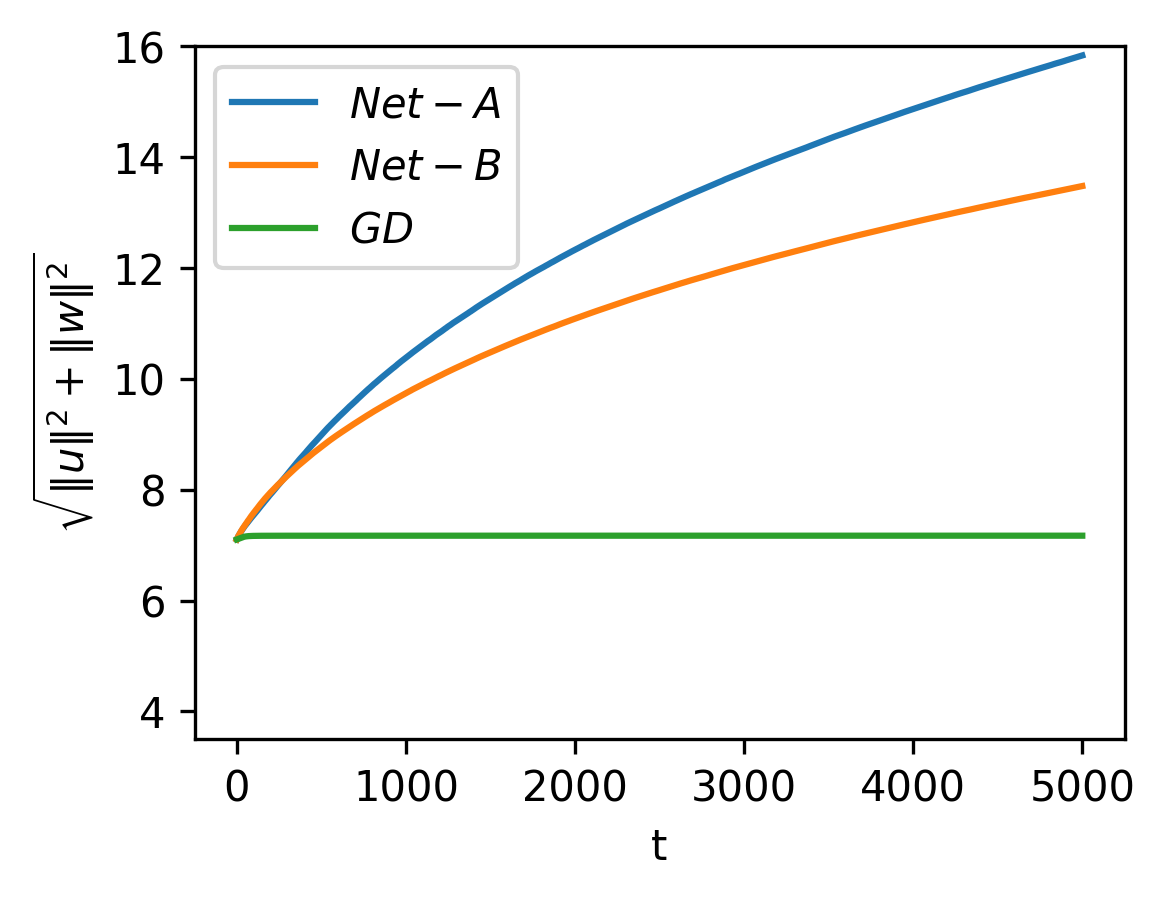
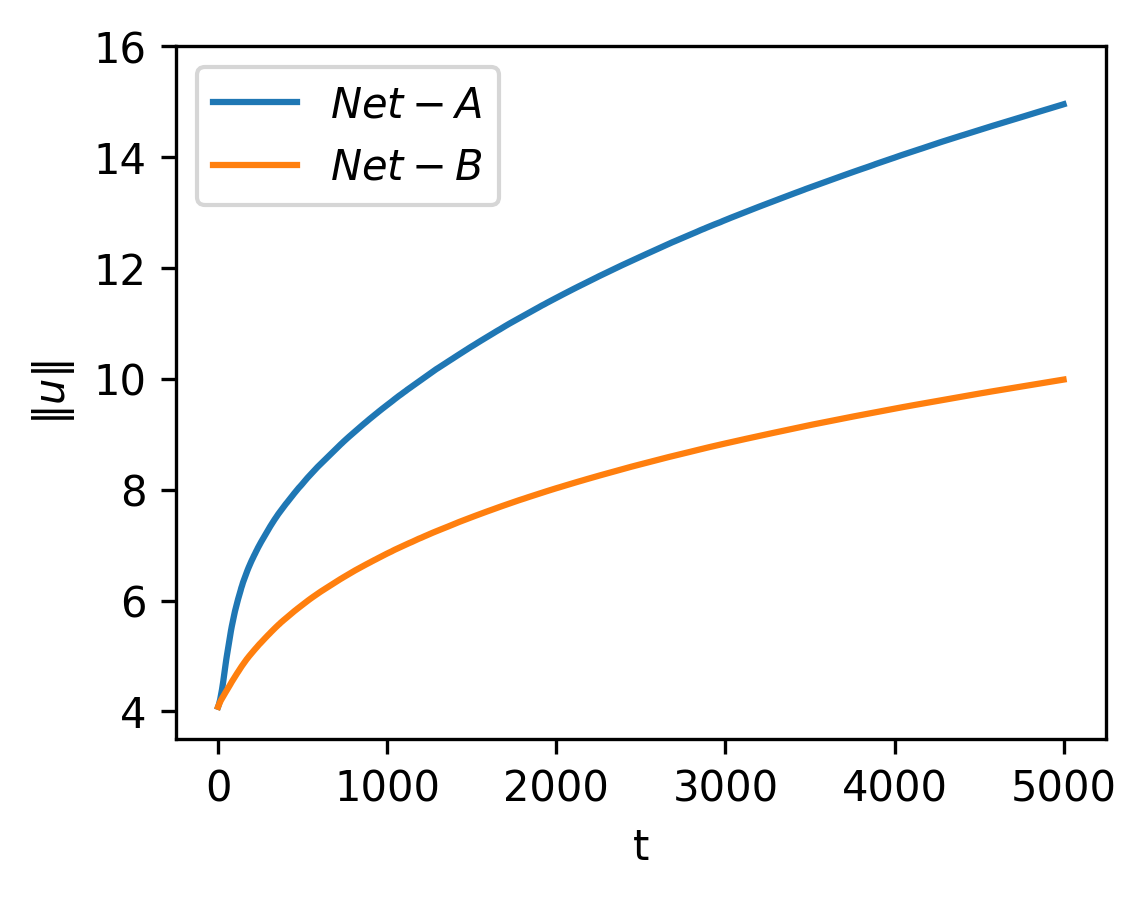
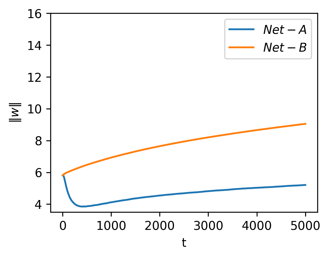
Figure 2: When there is scaling symmetry, the norm of the parameters increases monotonically under SGD but remains unchanged under GD. Left: evolution of the total model norm for two-layer nonlinear networks where there is a rescaling symmetry. Mid: evolution of the second layer. Right: evolution of the first layer. This shows that the evolution of each layer can be vastly different, but the total norm of the parameters with the scaling symmetry is always monotonically increasing. Also, note that for net $B$, each layer also has the rescaling symmetry, and so the norm of each layer for net-$B$ is also increasing. In contrast, net-$A$ does not have the layer-wise symmetry, and the individual norms can be either increasing or decreasing.

Let us start with a controlled experiment for the simplest case. The scale invariance appears when common normalization techniques such as batch normalization (Ioffe and Szegedy,, 2015) and layer normalization (Ba et al.,, 2016) are used. Let $\ell(\theta,x)$ denote a per-sample loss such that for any $\rho\in\mathbb{R}^{+}$: $\ell(\theta,x)=\ell(\rho\theta,x)$, where $\theta\in\mathbb{R}^{d}$. For this symmetry, $A=I$. Thus, by Eq. (7), we have during SGD training that

$$\frac{\mathop{}\!\mathrm{d}}{\mathop{}\!\mathrm{d}t}\|\theta_{t}\|^{2}=-\gamma\|\theta_{t}\|^{2}+\sigma^{2}{\rm Tr}[\Sigma(\theta_{t})].$$ (11)

Thus, without weight decay, the parameter norm increases monotonically and even diverges, particularly for under-parameterized models where the gradient noise is typically non-degenerate.

Here, we numerically compare two networks trained on GD and SGD: Net-A: $f(x)=\sum_{j}\frac{u_{j}}{\|w\|}\tanh({w_{j}^{T}}x/{\|u\|_{F}})$; and Net-B: $f(x)=\sum_{j}\frac{u_{ij}}{\|u\|}\tanh({w_{j}^{T}}x/{\|w\|_{F}})$. Here, $w$ and $u$ are matrices and $w_{j}$ denotes the $j$-th row of $w$ and $u_{j}$ denotes the $j$-th column of $u$. The two networks are different functions of $u$ and $w$. However, both networks have the global scale invariance: if we scale both $U$ and $W$ by an arbitrary positive scalar $\rho$, the network output and loss function remain unchanged for any sample $x$. We train these two networks on simple linear Gaussian data with GD or SGD. Figure 2 shows the result. Clearly, for SGD, both networks have a monotonically increasing norm, whereas the norm remains unchanged when the training proceeds with GD. What’s more, Net-B has two additional layer-wise scale invariances where one can scale only $u$ (or only $w$) by $\rho$ while keeping the loss function unchanged. This means that both layers will have a monotonically increasing norm, which is not the case for Net-A.

Recent works have studied the dynamics of SGD under the scale-invariant models when weight decay is present (Wan et al.,, 2021; Li et al.,, 2020). Our result shows that the model parameters will diverge without weight decay, leading to potential numerical problems. Combining the two results, the importance of having weight decay becomes clear: it prevents the divergence of models.

4.2 Generalized Matrix Factorization

exponential symmetry is also observed when the model involves a (generalized) matrix factorization. This occurs in standard matrix completion problems (Srebro et al.,, 2004) or within the self-attention of transformers through the key and query matrices (Vaswani et al.,, 2017). For a (generalized) matrix factorization problem, we have the following symmetry in the objective:

$$\ell(U,W,\theta^{\prime})=\ell(UA,A^{-1}W,\theta^{\prime})$$ (12)

for any invertible matrix $A$. We can consider the types of $A$ that is perturbatively away from identity: $A=I+\rho B+O(\rho^{2})$, and $A^{-1}=I-\rho B+O(\rho^{2})$. Therefore, for an arbitrary symmetric $B$, we have a conserved quantity for GD: $C_{B}(\theta)={\rm Tr}[UBU^{T}]-{\rm Tr}[W^{T}BW].$ This conservation law can also be written in the matrix form, which is well-known for GD (Du et al.,, 2018; Marcotte et al.,, 2023):

$$(W_{t}W^{T}_{t}-U_{t}^{T}U_{t})=(W_{0}W^{T}_{0}-U^{T}_{0}U_{0}).$$ (13)

For SGD, applying (5) gives the following proposition.

Proposition 1.

Suppose the symmetry (12) holds. Let $U=(\tilde{u}_{1},\cdots,\tilde{u}_{d_{2}})^{\top}\in\mathbb{R}^{d_{2}\times d}$, $W=(\tilde{w}_{1},\cdots,\tilde{w}_{d_{0}})\in\mathbb{R}^{d\times d_{0}}$, where $\tilde{u}_{i},\tilde{w}_{j}\in\mathbb{R}^{d}$. Let $C_{B}(\theta)={\rm Tr}[UBU^{T}]-{\rm Tr}[W^{T}BW]$ for any symmetruc matrix $B\in\mathbb{R}^{d\times d}$. Then, for SGD, we have

$$\dot{C}_{B}(\theta_{t})=\sigma^{2}\left(\sum_{i=1}^{d_{2}}{\rm Tr}[\Sigma_{\tilde{u}_{i}}(\theta_{t})B]-\sum_{j=1}^{d_{0}}{\rm Tr}[\Sigma_{\tilde{w}_{j}}(\theta_{t})B]\right).$$

For diagonal $B$ matrices, this solution reduces to the previous result found in Ziyin et al., 2023a . This problem is rather easily solvable when $U\in\mathbb{R}^{1\times d}$ and $W\in\mathbb{R}^{d\times 1}$. In this case, taking $B=E_{k,l}+E_{l,k}$ where $E_{i,j}$ denotes the matrix with entries of $1$ at $(i,j)$ and zeros elsewhere. For this choice of $B$, we obtain that $C_{B}(\theta)=W_{k}W_{l}-U_{k}U_{l}$, and applying the results we have derived, it is easy to show that for some random variable $r$: $\dot{C}_{B}(\theta_{t})=-{\rm Var}[r(\theta_{t})]C_{B}(\theta_{t}),$ which signals a exponential decay. For common problems, ${\rm Var}[r(\theta_{t})]>0$ (Ziyin et al., 2023a, ). Since the choice of $B$ is arbitrary, we have that $W_{k}W_{l}\to U_{k}U_{l}$ for all $k$ and $l$. The message is rather striking: SGD automatically converges to a solution where all neurons outputs the same sign (${\rm sgn}(U_{i}W_{i})={\rm sgn}(U_{j}W_{j})$) at an exponential rate.

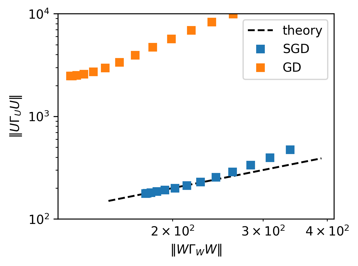
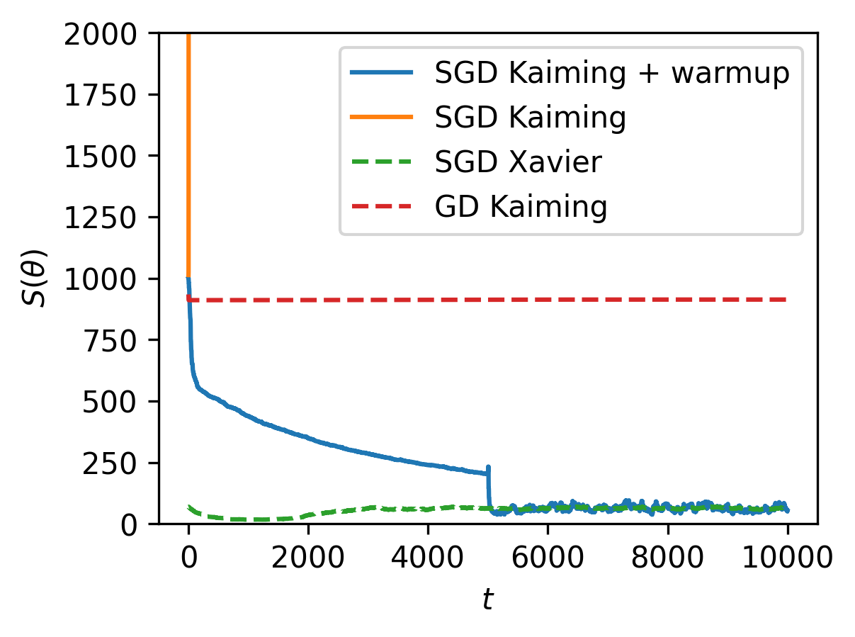
Figure 3: Comparison between GD and SGD for matrix factorizations. Left: converged solutions of SGD agree with the prediction of Theorem 2, but is an order of magnitude away from the solution found by GD, even if they start from the same init.. Right: Dynamics of the stability condition $S$ during the training of a rank-1 matrix factorization problem. The solid lines show the training of SGD with Kaiming init. When the learning rate ($\eta=0.008$) is too large, SGD diverges (orange line). However, when one starts training at a small learning rate ($0.001$) and increases $\eta$ to $0.008$ after 5000 iterations, the training remains stable. This is because SGD training improves the stability condition during training, in agreement with the theory. In contrast, the stability condition of GD and that of SGD with a Xavier init increases only slightly. Also, note that both Xavier and Kaiming init. under SGD converges to the same stability condition, also in agreement with the theory.

4.3 Balance and Stability of Matrix Factorization

To provide more concrete insights, let us consider a two-layer linear network (this can also be seen as a variant of standard matrix factorizations):

$$\ell_{\gamma}=\|UWx-y\|^{2}+\gamma(\|U\|_{F}^{2}+\|W\|_{F}^{2}).$$ (14)

where $x\in\mathbb{R}^{d_{x}}$ is the input data, and $y=y^{\prime}+\epsilon\in\mathbb{R}^{d_{y}}$ is a noisy version of the label. The ground truth mapping is linear and realizable: $y^{\prime}=U^{*}W^{*}x$. The second moments of the input and noise are denoted as $\Sigma_{x}=\mathbb{E}[xx^{T}]$ and $\Sigma_{\epsilon}=\mathbb{E}[\epsilon\epsilon^{T}]$, respectively.

The following theorem gives the fixed point of Noether flow.

Theorem 2.

Let $r=UWx-y$ be the prediction residual. Then, for any fixed $B$, $\dot{C}_{B}=0$ if

$$W\Gamma_{W}W^{T}=U^{T}\Gamma_{U}U,$$ (15)

where $\Gamma_{W}=\mathbb{E}[\|r\|^{2}xx^{T}]+2\gamma I$, $\Gamma_{U}=\mathbb{E}[\|x\|^{2}rr^{T}]+2\gamma I$.

The balance condition takes a more suggestive form when the model is at the global minimum, where $U^{*}W^{*}x-y=\epsilon$. Assuming that $\epsilon$ and $x$ are independent and that there is no weight decay, we have:

$$W\bar{\Sigma}_{x}W^{T}=U^{T}\bar{\Sigma}_{\epsilon}U$$ (16)

Here, the bar over the matrices indicates that they have been normalized by their traces: $\bar{\Sigma}=\Sigma/{\rm Tr}[\Sigma]$. The matrices $\Gamma_{W}$ and $\Gamma_{U}$ simplifies because at the global minimum, $r_{i}=\epsilon_{i}$ and so $\mathbb{E}[\|x\|^{2}rr^{T}]={\rm Tr}[\Sigma_{x}]\Sigma_{\epsilon}$ and $\mathbb{E}[\|r\|^{2}xx^{T}]={\rm Tr}[\Sigma_{\epsilon}]\Sigma_{x}$. This condition should be compared with the alignment condition for GD in Eq. (13), where perfect alignment is never possible and completely depends on the initialization. This condition simplifies further if both $\bar{\Sigma}_{x}$ and $\bar{\Sigma}_{\epsilon}$ are isotropic, where the equation simplifies to $WW^{T}/d_{x}=U^{T}U/d_{y}$. Namely, the two layers will be perfectly aligned, and the overall balance depends only on input and output dimensions. Figure 3-left shows an experiment that directly confirms the prediction of Theorem 2. Here, every point corresponds to the converged solution of an independent run with the same initialization and training procedures but different values of $\Sigma_{\epsilon}$. In agreement with the theory, the two layers are aligned according to Theorem 2 under SGD, but not under GD. In fact, GD finds solutions that are more than an order of magnitude away from SGD.

An important usage of this result is to explain both why warmup is effective in training neural networks (where progressive flattening happens) and why progressive sharpening happens (Jastrzebski et al.,, 2019), which can, in turn, be used to understand the edge of stability (Wu et al.,, 2018; Cohen et al.,, 2021). To see this, we first derive a metric of stability condition for this model.

Proposition 2.

For the per-sample loss (14), let $S(\theta):={\rm Tr}[\nabla^{2}L(\theta)]$. Then, $S(\theta)=d_{y}\|W\Sigma_{x}^{1/2}\|_{F}^{2}+\|U\|_{F}^{2}{\rm Tr}[\Sigma_{x}]$.

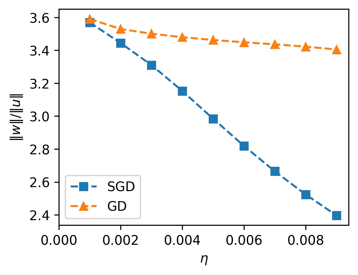
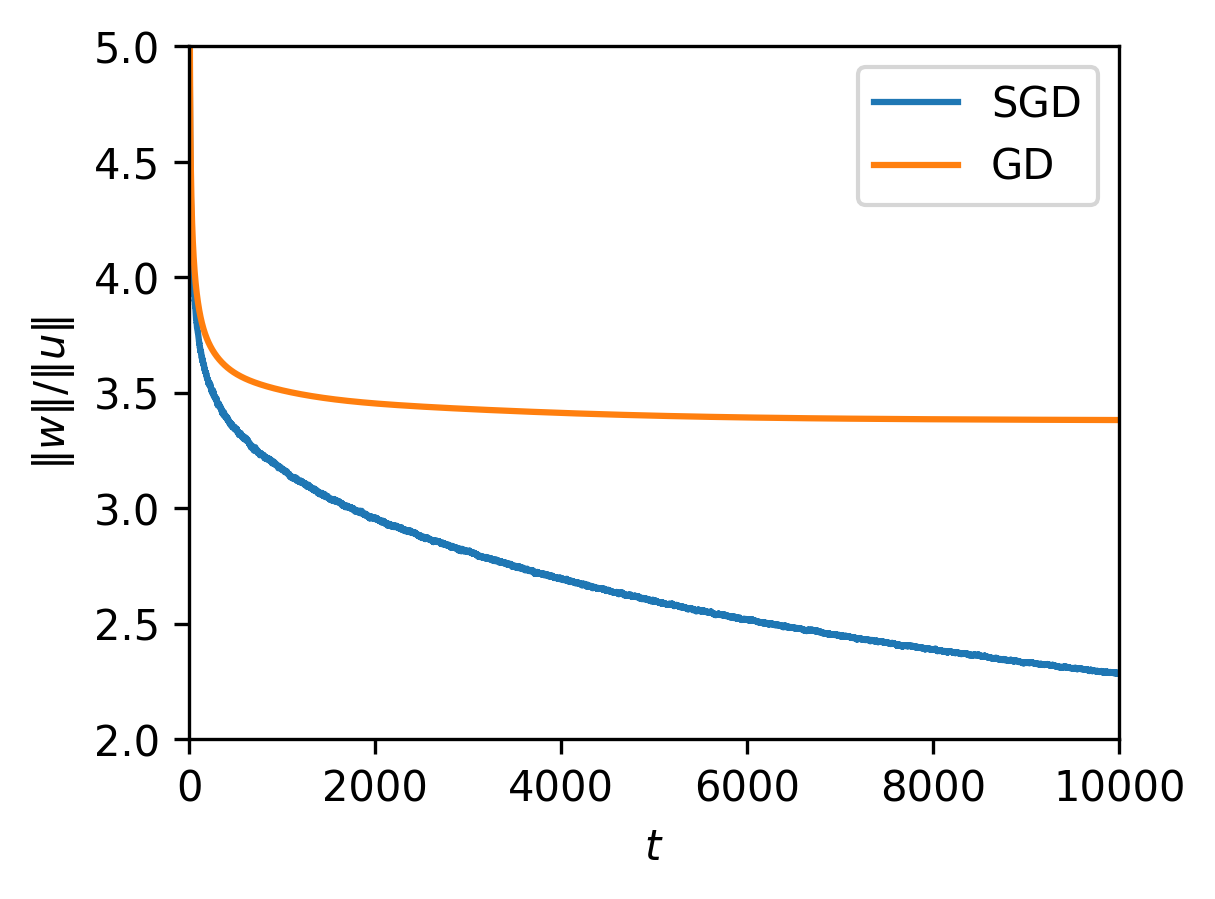
Figure 4: Training of a deep linear residual network under SGD and GD. When SGD is used, the model is biased towards a more balanced solution in comparison with GD training training. Left: the norm ratio between the two layers after training at different learning rates. The learning rate has a negligible effect on the norm ratio for the solution found by GD. In contrast, the solution found by SGD has more and more balanced borm under SGD when the training proceeds under a higher learning rate. It is clear that when the learning rate is small, the deviation from the GD is also small and linear in $\eta$, in agreement with the theory. Right: Example of learning dynamics for a fixed learning rate of $\eta=0.01$.

The trace of the Hessian is a good metric of the local stability of the GD and SGD algorithm because the trace upper bounds the largest Hessian eigenvalue. For a random Gaussian initialization with variance $\Gamma_{W}^{2}$ and $\Gamma_{U}^{2}$, the trace at initialization is, in expectation,

$$S_{\rm init}=d_{y}d{\rm Tr}[\Sigma_{x}](\Gamma_{W}^{2}+\Gamma_{U}^{2}).$$

Let us analyze the simplest case of an autoencoding task, where the model is close to the global minimum, $y^{\prime}=x$, and $\Sigma_{x}\propto I_{d_{x}}$, $\Sigma_{\epsilon}\propto I_{d_{y}}$. At the end of the training, the model is close to the global minimum and satisfies Proposition 2. Here, the rank of $U$ and $W$ matters and is upper bounded by $\min(d,d_{x})$, and at the global minimum, $U$ and $W$ are full-rank (equal to $\min(d,d_{x})$), and all the singular values are $1$. Thus, we have that

$$\begin{cases}S_{\rm init}=d_{x}d(\Gamma_{U}^{2}+\Gamma_{W}^{2}){\rm Tr}[\Sigma_{x}],\\ S_{\rm end}=2\min(d,d_{x}){\rm Tr}[\Sigma_{x}].\end{cases}$$ (17)

The change of the stability condition thus depends crucially on the initialization scheme. For Xavier init, $\Gamma_{U}^{2}=(d_{y}+d)^{-1}$ and $\Gamma_{W}^{2}=(d+d_{x})^{-1}$. Therefore, we have that $S_{\rm init}\approx S_{\rm end}$ (but $S_{\rm init}$ slightly smaller), which suggests that for the Xavier init., the sharpness of loss experiences a small sharpening during training (but not by much, and so it often appears roughly unchanged). For Kaiming init., $\Gamma_{U}^{2}=1$ and $\Gamma_{W}^{2}=d_{x}^{-1}$. Therefore, it always holds that $S_{\rm init}\geq S_{\rm end}$, and so the stability improves as the training proceeds. The only case when the Kaiming init. does not experience progressive flattening is when $d=d_{x}=d_{y}$, which agrees with the common observation that training is easier if the widths of the model are balanced (Hanin and Rolnick,, 2018). See Figure 3-right for an experiment when $d=1$, where progressive flattening of Kaiming init. is the most significant. A major technique that our theory can explain is using warmup to stabilize training in the early stage. This technique was first proposed in Goyal et al., (2017) for training CNNs, where it was observed that the training is divergent if we start the training at a fixed large learning rate $\eta_{\max}$. However, this divergent behavior disappears if we perform a warmup training, where the learning rate is increased gradually from a minimal value to $\eta_{\max}$. Later, the same technique is found to be crucially useful for training large language models (Popel and Bojar,, 2018). Before our work, almost no theory explained why warmup is helpful in training, and our result fills an important gap in this regard.

Also, Theorem 2 also offers a unified theory for explaining both the progressive sharpening and the progressive flattening: the sharpness of SGD after training depends on the alignment of the model with the distribution of data and noise, which in turn, decided by the fixed point of SGD. Depending on the data distribution, the alignment can both increase and decrease the sharpness.

4.4 Lack of Symmetry and Bias of SGD

Now, let us briefly consider what happens if the loss function does not have the symmetry. Here, we focus on the qualitative behavior and leave the complete analysis to future work. As a minimal model, let us consider the following loss function: $\ell=\ell_{1}(\theta,x)+\zeta\ell_{2}(\theta)$. Here, $\ell_{1}$ has the $A$-symmetry, whereas $\ell_{2}(\theta)$ has no symmetry nor randomness and so $\ell_{2}$ does not affect $\Sigma$ at all. $\zeta$ determines the relative strength between the two terms. In totality, $\ell$ no longer has the $A$-symmetry.

As previously, let $C_{A}=\theta^{\top}A\theta$ be $A$. Then,

$$\dot{C}_{A}(\theta)=-\zeta(\nabla\ell_{2})^{\top}A\theta^{*}+\eta{\rm Tr}[\Sigma(\theta)A],$$ (18)

whose fixed point is

$$\zeta(\nabla\ell_{2})^{\top}A\theta^{*}={\rm Tr}[\Sigma(\theta)A].$$ (19)

This balance condition thus depends strongly on how large $\zeta$ is. When $\zeta$ is perturbatively small, we see that SGD still favors the fixed point given by Theorem 1, but with a first-order correction in $\zeta$.

Conversely, if $\zeta$ is very large and $\sigma^{2}$ is very small, we can expand around a local minimum of the loss function $\theta^{*}$, and so the fixed point becomes

$$\zeta(\theta-\theta^{*})^{\top}H(\theta^{*})A\theta^{*} =\sigma^{2}{\rm Tr}[\Sigma(\theta^{*})A]$$

$$+O(\sigma^{2}\|\theta-\theta^{*}\|+\|\theta-\theta^{*}\|^{2}),$$ (20)

where $H$ is the Hessian of the empirical loss $\ell_{2}$. Certainly, this implies that SGD will stay around a point that deviates from the local minimum by an $O(\eta)$ amount. This stationary point potentially has many solutions. For example, one class of solution is when $\theta-\theta^{*}$ is an eigenvector of $H$ with eigenvalue $h^{*}>0$ and eigenvector $n$, we can denote $s=(\theta-\theta^{*})^{T}m$ obtain a direct solution on $s$:

$$s=\frac{\eta{\rm Tr}[\Sigma(\theta^{*})A]}{h^{*}n^{T}A\theta^{*}},$$ (21)

certainly, this deviation disappears in the limit $\sigma^{2}\to 0$. Therefore, this implicit regularization effect is only a consequence of SGD training and is not present under GD. With this condition, one can obtain a clean expression of the deviation of the quantity $C$ from its local minimum value $C^{*}:=(\theta^{*})^{T}A\theta^{*}$. We have that

$$C(\theta) =C^{*}+2(\theta-\theta^{*})^{T}A\theta^{*}+O(\|\theta-\theta^{*}\|^{2})$$ (22)

$$=C^{*}+2\frac{\eta}{h^{*}}{\rm Tr}[\Sigma A].$$ (23)

This shows that our results in the previous section are still qualitatively correct. The quantity $C$ will be systematically larger than the local minimum values of $C$ if the approximate symmetry matrix $A$ is PD. It is systematically smaller if $A$ is ND. When $A$ contains both positive and negative eigenvalues, the deviation of $C$ depends on the local gradient fluctuation balancing condition. Also, note that when the smallest eigenvalue of $H$ is close to zero (which is true for common neural networks), the dominant factor that biases $C$ occurs in this space. Therefore, it is, in general, not a bad idea to approximate the deviation as $C(\theta)\approx C^{*}+2\frac{\eta}{h_{\min}}{\rm Tr}[\Sigma A],$ where $h_{\min}$ is the smallest eigenvalue of the Hessian at the local minimum. In reality, $\zeta$ is neither too large nor too small, and one expects that the solution favored by SGD is an effective interpolation between the true local minimum and the fixed point favored by the symmetries.

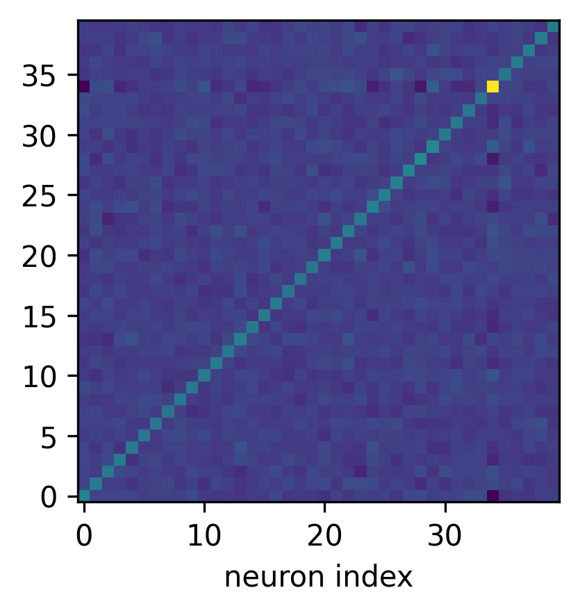
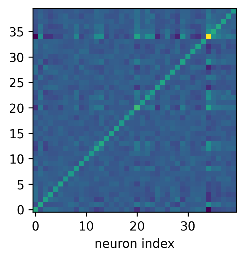
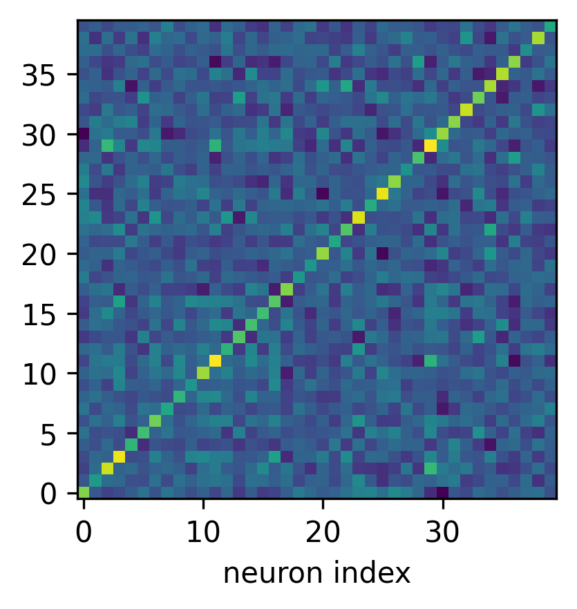
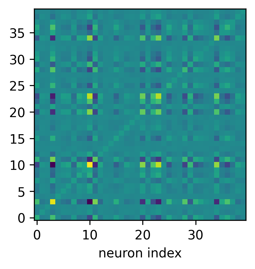
Figure 5: The latent representations of a two-layer tanh net trained under SGD (left) are similar across different layers, in agreement with the theory. However, the learned representations are dissimilar under GD (right). Here, we plot the matrices $W\bar{\Sigma}_{x}W$ (first and third plots) and $U\bar{\Sigma}_{\epsilon}U$ (second and fourth plots). Note that the quantity $W\bar{\Sigma}_{x}W$ is equal to the covariance of the preactivation representation of the first layer. This means that SGD and GD learn qualitatively different features after training.

A relevant and interesting example is when residual connections are used in a fully connected network. As a minimal model, consider the following residual deep linear network, where both $U$ and $W$ are square matrices of weights: $f(x)=(I+W)(I+U)x$. This network no longer has the rescaling symmetry. However, noticing that $(I+W)(I+U)=I+W+U+WU$, we see that the symmetry is partially exists in the model. We perform experiments on a dataset where both $x$ and $\epsilon$ have an isotropic covariance. According to the discussion in the previous section, SGD will converge to the most balanced solution after training if there are no residual connections. Thus, this implies that when trained with SGD, the network will have a more balanced norm than training under GD. Figure 4 shows that the theory agrees with the experiment.

Another example is shown in Figure 5, where we compare the latent representation of a two-layer tanh net with the prediction of 2. Tanh networks are a very natural example to compare against linear networks because, in many ways, they are close to a linear network. For example, when the parameters are close to zero, a tanh network is approximately linear and thus has the desired symmetries. Also, the tanh activation is strictly monotonic and thus qualitatively similar to a linear activation. Also, the quantity $W\bar{\Sigma}_{x}W$ has a very clean interpretation as the normalized covariance matrix of pre-activation hidden representation. Here, the task is a simple autoending task, where $x\in\mathbb{R}^{40}$ and $y=x+\epsilon$. $x$ is sampled from an isotropic Gaussian, and $\epsilon$ is an independent non-isotropic (but diagonal) Gaussian noise such that ${\rm Var}[\epsilon_{1}]=5$ and ${\rm Var}[\epsilon_{i}]=1$ for $i\neq 1$. We train with SGD or GD for $10^{4}$ iterations. The experimental results show that if trained with SGD, the learned representation agrees with the prediction of Theorem 2 very well, whereas under GD, the model learned a completely different representation. This suggests that our result may be greatly useful for understanding the structures of latent representations of trained neural networks.

5 Related Works

Very few works study the dynamics of SGD in the degenerate directions of the loss landscape. There are two closely related prior works. Ziyin et al., 2023a studies the dynamics of SGD when there is a simple rescaling symmetry and applies it to derive the stationary distribution of SGD for linear networks. In our framework, this setting corresponds to the special case of the symmetric matrix $A$ being a diagonal matrix where some of the diagonal elements are one while others are zero. Another highly related work is Li et al., (2020), which studies the dynamics of continuous-time SGD in the presence of simple scale invariance and weight decay. In the analysis, this work assumes the existence of the fixed point of the dynamics, which we proved the existence of, and does not consider the far larger family of invariance with respect to generic exponential maps. Also related is the study of conservation laws under gradient flow (Tanaka and Kunin,, 2021; Marcotte et al.,, 2023), which we have discussed in Section 3. A main limitation of these works is that they do not take the stochasticity of minibatch sampling into account. As a main implication of our theory, GD and SGD have a non-perturbative essential difference even if the minibatch noise is perturbatively small.

Wu et al., (2018) and Wu et al., (2022) shows that the same global minima can exhibit different stabilities for GD and so GD and SGD naturally prefer different solutions. Further, Blanc et al., (2020) and Li et al., 2021b propose a diffusion-based model to describe SGD’s exploration process on the global minima manifold. For a comprehensive survey of this topic, we refer to Vardi, (2023) the references therein. Our results are different from this line of works as our main focus is on the symmetry.

6 Conclusion

In this work, we have studied the common continuous symmetries, such as the rescaling symmetry and the scaling symmetry in deep learning in a unified perspective. We constructed the theoretical frameworks of exponential symmetries to study the special tendency of SGD to stay close to a special fixed point along the degenerate directions in the loss landscape. We proved that every exponential symmetry leads to a unique and essentially attractive fixed point in the degenerate direction. This point also has a clean interpretation: it is the point where the gradient noises of SGD in different subspaces balance and align. A major advantage of our result is that it only relies on the existence of symmetries and is independent of the particular definitions of model architecture or data distribution.

  Appendix  

Appendix A Proofs

A.1 Ito’s Lemma and Derivation of Eq. (5)

Let a vector $X_{t}$ follow the following stochastic process:

$$\mathop{}\!\mathrm{d}X_{t}=\mu_{t}\mathop{}\!\mathrm{d}t+G_{t}\mathop{}\!\mathrm{d}W_{t}$$ (24)

for a matrix $G_{t}$. Then, the dynamics of any function of $X_{t}$ can be written as (Ito’s Lemma)

$$\mathop{}\!\mathrm{d}f(X_{t})=\left(\nabla_{X}^{\top}f\mu_{t}+\frac{1}{2}{\rm Tr}[G_{t}^{\top}\nabla^{2}f(X_{t})G_{t}]\right)\mathop{}\!\mathrm{d}t+\nabla f(X_{t})^{\top}G_{t}\mathop{}\!\mathrm{d}W_{t}.$$ (25)

Applying this result to quantity $C(\theta)$ under the SGD dynamics, we obtain that

$$dC=\left(\nabla^{\top}C\nabla L+\frac{\sigma^{2}}{2}{\rm Tr}[\Sigma(\theta)\nabla^{2}C]\right)dt+\nabla^{\top}C\sqrt{\sigma^{2}\Sigma(\theta)}dW_{t},$$ (26)

where we have used $\mu_{t}=\nabla L$, $G_{t}=\sqrt{\sigma^{2}\Sigma(\theta)}$. By Eq. (3), we have that

$$\nabla^{\top}C\nabla L=\mathbb{E}[\nabla^{\top}C\nabla\ell]=0,$$ (27)

and

$$\nabla^{\top}C\Sigma=\mathbb{E}[\nabla^{\top}C\nabla\ell\nabla^{\top}\ell]-\mathbb{E}[\nabla^{\top}C\nabla\ell]\mathbb{E}[\nabla^{\top}\ell]=0.$$ (28)

Because ${\Sigma(\theta)}$ and $\sqrt{\Sigma(\theta)}$ share eigenvectors, we have that

$$\nabla^{\top}C\sqrt{\sigma^{2}\Sigma(\theta)}=0.$$ (29)

Therefore, we have derived:

$$dC=\frac{\sigma^{2}}{2}{\rm Tr}[\Sigma(\theta)\nabla^{2}C]dt.$$ (30)

A.2 Proof of Theorem 1

Proof.

First of all, let us establish the relationship between $\nabla\ell(\theta)$ and $\nabla\ell(\exp(\lambda A))$. By the definition of the quadrative symmetry, we have that for an arbitrary $\lambda$,

$$\ell(\theta)=\ell(e^{\lambda A}\theta).$$ (31)

Taking the derivative of both sides, we obtain that

$$\nabla_{\theta}\ell(\theta)=e^{\lambda A}\nabla_{\theta_{\lambda}}\ell(\theta_{\lambda}),$$ (32)

The standard result of Lie groups shows that $e^{\lambda A}$ is full-rank and symmetric, and its inverse is $e^{-\lambda A}$. Therefore, we have

$$e^{-\lambda A}\nabla_{\theta}\ell(\theta)=\nabla_{\theta_{\lambda}}\ell(\theta_{\lambda}).$$ (33)

Now, we apply this relation to the trace of interest. By definition,

$$\Sigma(\theta_{\lambda}) =\mathbb{E}[\nabla_{\theta_{\lambda}}\ell(\theta_{\lambda})\nabla_{\theta_{\lambda}}^{\top}\ell(\theta_{\lambda})]$$ (34)

$$=e^{-\lambda A}\Sigma(\theta)e^{-\lambda A}.$$ (35)

Because $e^{\lambda A}$ is a function of $A$, it commutes with $A$. Therefore,

$${\rm Tr}[\Sigma(\theta_{\lambda})A] ={\rm Tr}[e^{-\lambda A}\Sigma(\theta)e^{-\lambda A}A]$$ (36)

$$={\rm Tr}[e^{-2\lambda A}\Sigma(\theta)A].$$ (37)

Similarly, the regularization term is

$$\gamma\theta_{\lambda}^{\top}A\theta_{\lambda}=\gamma{\rm Tr}[\theta^{\top}\theta Ae^{2\lambda A}]$$ (38)

Now, if ${\rm Tr}[\Sigma(\theta)A]=\theta^{\top}A\theta=0$, we have already proved item (2) of the theorem. Therefore, let us consider the case when either (or both) ${\rm Tr}[\Sigma(\theta)A]\neq 0$ or $\theta^{\top}A\theta\neq 0$

Without loss of generality, we assume $\gamma\geq 0$, and the case of $\gamma<0$ follows an analogous proof. In such a case, we can write the trace in terms of the eigenvectors $n_{i}$ of $A$:

$$-\gamma\theta_{\lambda}^{\top}A\theta_{\lambda}+\eta{\rm Tr}[\Sigma(\theta_{\lambda})A] =\underbrace{\eta\sum_{\mu_{i}>0}e^{-2\lambda|\mu_{i}|}|\mu_{i}|\sigma_{i}^{2}+\gamma\sum_{\mu_{i}<0}e^{-2\lambda|\mu_{i}|}|\mu_{i}|\tilde{\theta}_{i}^{2}}_{I_{1}(\lambda)}-\underbrace{\left(\eta\sum_{\mu_{i}<0}e^{2\lambda|\mu_{i}|}|\mu_{i}|\sigma_{i}^{2}+\gamma\sum_{\mu_{i}>0}e^{2\lambda|\mu_{i}|}|\mu_{i}|\tilde{\theta}_{i}^{2}\right)}_{I_{2}(\lambda)}$$

$$=:I(\lambda),$$

where $\mu_{i}$ is the $i$-th eigenvalue of $A$, $\tilde{\theta}_{i}=(n_{i}^{\top}\theta_{i})^{2}$, $\sigma_{i}^{2}=n_{i}^{\top}\Sigma(\theta)n_{i}\geq 0$ is the norm of the projection of $\Sigma$ in this direction.

By definition, $I_{1}$ is either a zero function or strictly monotonically increasing function with $I_{1}(-\infty)=+\infty,I_{1}(+\infty)=0$ Likewise, $I_{2}$ is either a zero function or a strictly monotonically increasing function with $I_{2}(-\infty)=0,I_{2}(+\infty)=+\infty$. By the assumption ${\rm Tr}(\Sigma(\theta)A)\neq 0$ or ${\rm Tr}(\theta\theta^{\top}A)\neq 0$, we have that at least one of $I_{1}$ and $I_{2}$ must be a strictly monotonic function.

• If $I_{1}$ or $I_{2}$ is zero, we can take $\lambda$ to be either $+\infty$ or $-\infty$ to satisfy the condition.

• If both $I_{1}$ and $I_{2}$ are nonzero, then $I=I_{1}-I_{2}$ is a strictly monotonically decreasing function with $I(-\infty)=+\infty$ and $I(+\infty)=-\infty$. Therefore, there must exist only a unique $\lambda^{*}\in\mathbb{R}$ such that $I(\lambda^{*})=0$.

For the proof of (4), we denote the multi-variable function $J(\theta;\lambda):=G(\theta_{\lambda})$. Given that $\Sigma(\theta)$ is differentiable, $\frac{\partial J}{\partial\theta}$ exists.

It is easy to see that $\frac{\partial J}{\partial\lambda}$ is continuous. Moreover, for any $\theta$ and $\lambda=\lambda^{*}(\theta)$,

$$-\frac{\partial J}{2\partial\lambda}=\eta\sum_{\mu_{i}>0}e^{-2\lambda|\mu_{i}|}|\mu_{i}|^{2}\sigma_{i}^{2}+\gamma\sum_{\mu_{i}<0}e^{-2\lambda|\mu_{i}|}|\mu_{i}|^{2}\tilde{\theta}_{i}^{2}+\eta\sum_{\mu_{i}<0}e^{2\lambda|\mu_{i}|}|\mu_{i}|^{2}\sigma_{i}^{2}+\gamma\sum_{\mu_{i}>0}e^{2\lambda|\mu_{i}|}|\mu_{i}|^{2}\tilde{\theta}_{i}^{2}\neq 0.$$

Consequently, according to the Implicit Function Theorem, the function $\lambda^{*}(\theta)$ is differentiable. Additionally, $\frac{\partial\lambda}{\partial\theta}=-\frac{\frac{\partial J}{\partial\theta}}{\frac{\partial J}{\partial\lambda}}$.

∎

A.3 Proof of Proposition 1

Proof.

Recall that $U=(\tilde{u}_{1},\cdots,\tilde{u}_{d_{2}})^{\top}\in\mathbb{R}^{d_{2}\times d}$, $W=(\tilde{w}_{1},\cdots,\tilde{w}_{d_{0}})\in\mathbb{R}^{d\times d_{0}}$, where $\tilde{u}_{i},\tilde{w}_{i}\in\mathbb{R}^{d}$. $\theta=\text{vec}(U,W)=(\tilde{u}_{1}^{\top},\cdots,\tilde{u}_{d_{2}}^{\top},\tilde{w}_{1}^{\top},\cdots,\tilde{w}_{d_{0}}^{\top})^{\top}\in\mathbb{R}^{(d_{2}+d_{0})d}$.

$$\dot{C}=\eta{\rm Tr}(\Sigma(\theta)\nabla_{\theta\theta}^{2}C),$$

For $\nabla_{\theta\theta}^{2}C$, it holds that

$$\nabla^{2}_{\tilde{u}_{i},\tilde{u}_{j}}C=\begin{cases}B,\ &i=j;\\ 0,\ &\text{otherwise}.\end{cases},\quad\nabla^{2}_{\tilde{w}_{i},\tilde{w}_{j}}C=\begin{cases}-B,\ &i=j;\\ 0,\ &\text{otherwise}.\end{cases}\quad\nabla^{2}_{\tilde{u}_{i},\tilde{w}_{j}}C=0.$$

Therefore,

$${\rm Tr}[\Sigma(\theta)\nabla_{\theta\theta}^{2}C]=\sum_{i=1}^{n}{\rm Tr}\left[\nabla_{\theta}\ell_{i}\nabla_{\theta}\ell_{i}^{\top}\nabla_{\theta\theta}^{2}C\right]=\sum_{i=1}^{n}\left(\sum_{k=1}^{d_{2}}{\rm Tr}\left[\nabla_{\tilde{u}_{k}}\ell_{i}\nabla_{\tilde{u}_{k}}\ell_{i}^{\top}B\right]-\sum_{l=1}^{d_{0}}{\rm Tr}\left[\nabla_{\tilde{w}_{l}}\ell_{i}\nabla_{\tilde{w}_{l}}\ell_{i}^{\top}B\right]\right)$$

$$= \sum_{k=1}^{d_{2}}{\rm Tr}[\Sigma(\tilde{u}_{k})B]-\sum_{l=1}^{d_{0}}{\rm Tr}[\Sigma(\tilde{w}_{l})B].$$

The proof is complete. ∎

A.4 Proofs of Proposition 2

Proof.

The loss function is

$$\ell=\|UWx-y\|^{2}+\gamma(\|U\|_{F}^{2}+\|W\|_{F}^{2}).$$

Let us adopt the following notation: $U=(\tilde{u}_{1},\cdots,\tilde{u}_{d_{y}})^{\top}\in\mathbb{R}^{d_{y}\times d}$, $W=(\tilde{w}_{1},\cdots,\tilde{w}_{d_{x}})\in\mathbb{R}^{d\times d_{x}}$, where $\tilde{u}_{i},\tilde{w}_{i}\in\mathbb{R}^{d}$. $\theta=\text{vec}(U,W)=(\tilde{u}_{1}^{\top},\cdots,\tilde{u}_{d_{y}}^{\top},\tilde{w}_{1}^{\top},\cdots,\tilde{w}_{d_{x}}^{\top})^{\top}\in\mathbb{R}^{(d_{x}+d_{y})d}$.

Due to

$$\nabla_{\tilde{u}_{i}}\ell=Wx(\tilde{u}_{i}^{\top}Wx-y_{i})+2\gamma\tilde{u}_{i},\quad\forall i\in[d_{y}];$$

$$\nabla_{\tilde{w}_{j}}\ell=\sum_{i=1}^{d_{y}}\tilde{u}_{i}x_{j}\left(\tilde{u}_{i}^{\top}Wx-y_{i}\right)+2\gamma\tilde{w}_{j},\quad\forall j\in[d_{x}];$$

the diagonal blocks of the Hessian $\nabla_{\theta\theta}^{2}\ell$ have the following form:

$$\nabla_{\tilde{u}_{i},\tilde{u}_{i}}^{2}\ell=Wxx^{\top}W^{\top}+2\gamma I,\quad\forall i\in[d_{y}];$$

$$\nabla_{\tilde{w}_{j},\tilde{w}_{j}}^{2}\ell=x_{j}^{2}\sum_{i=1}^{d_{y}}\tilde{u}_{i}\tilde{u}_{i}^{\top}+2\gamma I,\quad\forall j\in[d_{x}].$$

The trace of the Hessian is a good metric of the local stability of the GD and SGD algorithm because the trace upper bounds the largest Hessian eigenvalue. For this loss function, the trace of the Hessian of the empirical risk is

$$S(U,W):={\rm Tr}[\nabla_{\theta\theta}^{2}\ell-2\gamma I]$$

$$= \sum_{i=1}^{d_{y}}{\rm Tr}[Wxx^{\top}W^{\top}]+\sum_{j=1}^{d_{x}}{\rm Tr}[x_{j}^{2}\sum_{i=1}^{d_{y}}\tilde{u}_{i}\tilde{u}_{i}^{\top}]$$

$$= d_{y}{\rm Tr}[W\Sigma_{x}W^{\top}]+\|U\|_{F}^{2}{\rm Tr}[\Sigma_{x}]=d_{y}\|W\Sigma_{x}^{1/2}\|_{F}^{2}+\|U\|_{F}^{2}{\rm Tr}[\Sigma_{x}],$$

where $\Sigma_{x}=xx^{\top}$. ∎

Appendix B Proof of Theorem 2

Proof.

First, we split $U$ and $W$ like $U=({u}_{1},\cdots,{u}_{d})\in\mathbb{R}^{d_{y}\times d}$ and $W=({w}_{1}^{\top},\cdots,{w}_{d}^{\top})^{\top}\in\mathbb{R}^{d\times d_{x}}$. The quantity under consideration is $C_{B}={\rm Tr}[UBU^{\top}]-{\rm Tr}[W^{\top}BW]$ for an arbitrary symmetric matrix $B$. What will be relevant to us is the type of $B$ that is indexed by two indices $k$ and $l$ such that

$$\begin{cases}B^{(k,l)}_{ij}=B^{(k,l)}_{ji}=1&\text{if $i=k$ and $j=l$ or $i=l$ and $j=k$};\\ B^{(k,l)}_{ij}=0&\text{otherwise}.\end{cases}$$ (39)

Specifically, for $k,l\in[d]$, we select $B^{(k,l)}_{i,j}=\delta_{i,k}\delta_{j,l}+\delta_{i,l}\delta_{j,k}$ in $C_{B}$. With this choice, for an arbitrary pair of $k$ and $l$,

$$C_{B^{(k,l)}}={u}_{k}^{\top}u_{l}-{w}_{k}^{\top}w_{l}.$$

and

$$W^{\top}B^{(k,l)}W=w_{k}w_{l}^{\top}+w_{l}w_{k}^{\top},$$ (40)

$$UB^{(k,l)}U^{\top}=u_{k}u_{l}^{\top}+u_{l}u_{k}^{\top},$$ (41)

Therefore,

$$\mathbb{E}\sum_{i=1}^{d_{y}}{\rm Tr}\left[\Sigma(\tilde{u}_{i})B^{(k)}\right] =\mathbb{E}\sum_{i=1}^{d_{y}}(\tilde{u}_{i}^{\top}Wx-y_{i})^{2}{\rm Tr}\left[Wxx^{\top}W^{\top}B^{(k)}\right]$$ (42)

$$=\mathbb{E}\left[\|r\|^{2}{\rm Tr}[Wxx^{\top}W^{\top}B^{(k,l)}]\right]$$ (43)

$$={\rm Tr}\left[\mathbb{E}[\|r\|^{2}xx^{\top}]W^{\top}B^{(k)}W\right]$$ (44)

$$={\rm Tr}[\Sigma_{W}^{\prime}(w_{k}w_{l}^{\top}+w_{l}w_{k}^{\top})]$$ (45)

$$=2w_{k}^{\top}\Sigma_{w}^{\prime}w_{l}$$ (46)

where we have defined $r_{i}=\tilde{u}_{i}^{\top}Wx-y_{i}$ and $\Sigma_{W}^{\prime}=\mathbb{E}[\|r\|^{2}xx^{\top}]$.

Likewise, we have that

$$\mathbb{E}\sum_{j=1}^{d_{x}}{\rm Tr}\left[\Sigma(\tilde{w}_{j})B^{(k)}\right] =\mathbb{E}\sum_{j=1}^{d_{x}}x_{j}^{2}{\rm Tr}\left[\left(\sum_{i=1}^{d_{y}}\tilde{u}_{i}(\tilde{u}_{i}^{\top}Wx-y_{i})\right)\left(\sum_{i=1}^{d_{y}}(\tilde{u}_{i}^{\top}Wx-y_{i})\tilde{u}_{i}^{\top}\right)B^{(k)}\right]$$

$$={\rm Tr}\left[\mathbb{E}[\|x\|^{2}U^{\top}rr^{\top}UB^{(k,l)}]\right]$$

$$={\rm Tr}[\Sigma_{U}^{\prime}UB^{(k,l)}U^{\top}]$$

$$=2u_{k}^{\top}\Sigma_{u}^{\prime}u_{l}.$$

where we have defined $\Sigma_{u}^{\prime}=\mathbb{E}[\|x\|^{2}rr^{\top}]$. Therefore, we have found that for arbitrary pair of $k$ and $l$

$$\dot{C}_{B^{(k,l)}}=-2\gamma(u_{k}^{\top}u_{l}-w_{k}^{\top}w_{l})+2\eta(w_{k}^{\top}\Sigma_{w}^{\prime}w_{l}-u_{k}^{\top}\Sigma_{u}^{\prime}u_{l}).$$ (47)

The fixed point of this dynamics is:

$$w_{k}^{\top}\Sigma_{w}w_{l}=u_{k}^{\top}\Sigma_{u}u_{l}.$$ (48)

where $\Sigma_{w}=\eta\Sigma_{w}^{\prime}+\gamma I$ and $\Sigma_{U}=\eta\Sigma_{u}^{\prime}+\gamma I$. Because this holds for arbitrary $k$ and $l$, the equation can be written in a matrix form:

$$W\Sigma_{w}W^{\top}=U^{\top}\Sigma_{u}U.$$ (49)

Let $V=UW$. To show that a solution exists for an arbitrary $V$. Let $W^{\prime}=W\sqrt{\Sigma_{w}}$ and $U^{\prime}=\sqrt{\Sigma_{u}}U$, which implies that

$$U^{\prime}W^{\prime}=\sqrt{\Sigma_{u}}V\sqrt{\Sigma_{w}}:=V^{\prime},$$ (50)

and

$$W^{\prime}(W^{\prime})^{\top}=(U^{\prime})^{\top}U^{\prime}.$$ (51)

Namely, $U^{\prime}$ and $(W^{\prime})^{\top}$ must have the same right singular vectors and singular values. This gives us the following solution. Let $V^{\prime}=LSR$ be the singular value decomposition of $V^{\prime}$, where $L$ and $R$ are orthogonal matrices an $S$ is a positive diagonal matrix. Then, for an arbitrary orthogonal matrix $F$, the following choice of $U^{\prime}$ and $W^{\prime}$ satisfies the two conditions:

$$\begin{cases}U^{\prime}=L\sqrt{S}F;\\ W^{\prime}=F^{\top}\sqrt{S}R.\end{cases}$$ (52)

This finishes the proof. ∎

References

- Ba et al., (2016) Ba, J. L., Kiros, J. R., and Hinton, G. E. (2016). Layer normalization. arXiv preprint arXiv:1607.06450.
- Blanc et al., (2020) Blanc, G., Gupta, N., Valiant, G., and Valiant, P. (2020). Implicit regularization for deep neural networks driven by an ornstein-uhlenbeck like process. In Conference on learning theory, pages 483–513. PMLR.
- Cohen et al., (2021) Cohen, J. M., Kaur, S., Li, Y., Kolter, J. Z., and Talwalkar, A. (2021). Gradient descent on neural networks typically occurs at the edge of stability. arXiv preprint arXiv:2103.00065.
- Dinh et al., (2017) Dinh, L., Pascanu, R., Bengio, S., and Bengio, Y. (2017). Sharp Minima Can Generalize For Deep Nets. ArXiv e-prints.
- Du et al., (2018) Du, S. S., Hu, W., and Lee, J. D. (2018). Algorithmic regularization in learning deep homogeneous models: Layers are automatically balanced. Advances in neural information processing systems, 31.
- Fontaine et al., (2021) Fontaine, X., Bortoli, V. D., and Durmus, A. (2021). Convergence rates and approximation results for sgd and its continuous-time counterpart. In Belkin, M. and Kpotufe, S., editors, Proceedings of Thirty Fourth Conference on Learning Theory, volume 134 of Proceedings of Machine Learning Research, pages 1965–2058. PMLR.
- Goyal et al., (2017) Goyal, P., Dollár, P., Girshick, R., Noordhuis, P., Wesolowski, L., Kyrola, A., Tulloch, A., Jia, Y., and He, K. (2017). Accurate, large minibatch sgd: Training imagenet in 1 hour. arXiv preprint arXiv:1706.02677.
- Hall and Hall, (2013) Hall, B. C. and Hall, B. C. (2013). Lie groups, Lie algebras, and representations. Springer.
- Hanin and Rolnick, (2018) Hanin, B. and Rolnick, D. (2018). How to start training: The effect of initialization and architecture. Advances in Neural Information Processing Systems, 31.
- Hu et al., (2017) Hu, W., Li, C. J., Li, L., and Liu, J.-G. (2017). On the diffusion approximation of nonconvex stochastic gradient descent. arXiv preprint arXiv:1705.07562.
- Ioffe and Szegedy, (2015) Ioffe, S. and Szegedy, C. (2015). Batch normalization: Accelerating deep network training by reducing internal covariate shift. arXiv preprint arXiv:1502.03167.
- Jastrzebski et al., (2019) Jastrzebski, S., Szymczak, M., Fort, S., Arpit, D., Tabor, J., Cho, K., and Geras, K. (2019). The break-even point on optimization trajectories of deep neural networks. In International Conference on Learning Representations.
- Jordan, (2018) Jordan, M. I. (2018). Dynamical, symplectic and stochastic perspectives on gradient-based optimization. In Proceedings of the International Congress of Mathematicians: Rio de Janeiro 2018, pages 523–549. World Scientific.
- Kunin et al., (2020) Kunin, D., Sagastuy-Brena, J., Ganguli, S., Yamins, D. L., and Tanaka, H. (2020). Neural mechanics: Symmetry and broken conservation laws in deep learning dynamics. arXiv preprint arXiv:2012.04728.
- Li et al., (2019) Li, Q., Tai, C., and E, W. (2019). Stochastic modified equations and dynamics of stochastic gradient algorithms i: Mathematical foundations. Journal of Machine Learning Research, 20(40):1–47.
- Li et al., (2020) Li, Z., Lyu, K., and Arora, S. (2020). Reconciling modern deep learning with traditional optimization analyses: The intrinsic learning rate. Advances in Neural Information Processing Systems, 33:14544–14555.
- (17) Li, Z., Malladi, S., and Arora, S. (2021a). On the validity of modeling sgd with stochastic differential equations (sdes).
- (18) Li, Z., Wang, T., and Arora, S. (2021b). What happens after sgd reaches zero loss?–a mathematical framework. In International Conference on Learning Representations.
- Liu et al., (2021) Liu, K., Ziyin, L., and Ueda, M. (2021). Noise and fluctuation of finite learning rate stochastic gradient descent.
- Marcotte et al., (2023) Marcotte, S., Gribonval, R., and Peyré, G. (2023). Abide by the law and follow the flow: Conservation laws for gradient flows.
- Noether, (1918) Noether, E. (1918). Invariante variationsprobleme. Königlich Gesellschaft der Wissenschaften Göttingen Nachrichten Mathematik-physik Klasse, 2:235–267.
- Pesme et al., (2021) Pesme, S., Pillaud-Vivien, L., and Flammarion, N. (2021). Implicit bias of sgd for diagonal linear networks: a provable benefit of stochasticity. Advances in Neural Information Processing Systems, 34:29218–29230.
- Popel and Bojar, (2018) Popel, M. and Bojar, O. (2018). Training tips for the transformer model. arXiv preprint arXiv:1804.00247.
- Salimans and Kingma, (2016) Salimans, T. and Kingma, D. P. (2016). Weight normalization: A simple reparameterization to accelerate training of deep neural networks. Advances in neural information processing systems, 29.
- Shirish Keskar et al., (2016) Shirish Keskar, N., Mudigere, D., Nocedal, J., Smelyanskiy, M., and Tang, P. T. P. (2016). On Large-Batch Training for Deep Learning: Generalization Gap and Sharp Minima. ArXiv e-prints.
- Sirignano and Spiliopoulos, (2020) Sirignano, J. and Spiliopoulos, K. (2020). Stochastic gradient descent in continuous time: A central limit theorem. Stochastic Systems, 10(2):124–151.
- Srebro et al., (2004) Srebro, N., Rennie, J., and Jaakkola, T. (2004). Maximum-margin matrix factorization. Advances in neural information processing systems, 17.
- Tanaka and Kunin, (2021) Tanaka, H. and Kunin, D. (2021). Noether’s learning dynamics: Role of symmetry breaking in neural networks. In Ranzato, M., Beygelzimer, A., Dauphin, Y., Liang, P., and Vaughan, J. W., editors, Advances in Neural Information Processing Systems, volume 34, pages 25646–25660. Curran Associates, Inc.
- Vardi, (2023) Vardi, G. (2023). On the implicit bias in deep-learning algorithms. Communications of the ACM, 66(6):86–93.
- Vaswani et al., (2017) Vaswani, A., Shazeer, N., Parmar, N., Uszkoreit, J., Jones, L., Gomez, A. N., Kaiser, Ł., and Polosukhin, I. (2017). Attention is all you need. Advances in neural information processing systems, 30.
- Wan et al., (2021) Wan, R., Zhu, Z., Zhang, X., and Sun, J. (2021). Spherical motion dynamics: Learning dynamics of normalized neural network using sgd and weight decay. Advances in Neural Information Processing Systems, 34:6380–6391.
- Wu et al., (2018) Wu, L., Ma, C., et al. (2018). How sgd selects the global minima in over-parameterized learning: A dynamical stability perspective. Advances in Neural Information Processing Systems, 31.
- Wu et al., (2022) Wu, L., Wang, M., and Su, W. (2022). The alignment property of SGD noise and how it helps select flat minima: A stability analysis. Advances in Neural Information Processing Systems, 35:4680–4693.
- Zhu et al., (2018) Zhu, Z., Wu, J., Yu, B., Wu, L., and Ma, J. (2018). The anisotropic noise in stochastic gradient descent: Its behavior of escaping from sharp minima and regularization effects. arXiv preprint arXiv:1803.00195.
- (35) Ziyin, L., Li, H., and Ueda, M. (2023a). Law of balance and stationary distribution of stochastic gradient descent. arXiv preprint arXiv:2308.06671.
- Ziyin et al., (2022) Ziyin, L., Liu, K., Mori, T., and Ueda, M. (2022). Strength of minibatch noise in SGD. In International Conference on Learning Representations.
- (37) Ziyin, L., Lubana, E. S., Ueda, M., and Tanaka, H. (2023b). What shapes the loss landscape of self supervised learning? In The Eleventh International Conference on Learning Representations.