GSINA: Improving Subgraph Extraction for Graph Invariant Learning via Graph Sinkhorn Attention

Abstract

Graph invariant learning (GIL) has been an effective approach to discovering the invariant relationships between graph data and its labels for different graph learning tasks under various distribution shifts. Many recent endeavors of GIL focus on extracting the invariant subgraph from the input graph for prediction as a regularization strategy to improve the generalization performance of graph learning. Despite their success, such methods also have various limitations in obtaining their invariant subgraphs. In this paper, we provide in-depth analyses of the drawbacks of existing works and propose corresponding principles of our invariant subgraph extraction: 1) the sparsity, to filter out the variant features, 2) the softness, for a broader solution space, and 3) the differentiability, for a soundly end-to-end optimization. To meet these principles in one shot, we leverage the Optimal Transport (OT) theory and propose a novel graph attention mechanism called Graph Sinkhorn Attention (GSINA). This novel approach serves as a powerful regularization method for GIL tasks. By GSINA, we are able to obtain meaningful, differentiable invariant subgraphs with controllable sparsity and softness. Moreover, GSINA is a general graph learning framework that could handle GIL tasks of multiple data grain levels. Extensive experiments on both synthetic and real-world datasets validate the superiority of our GSINA, which outperforms the state-of-the-art GIL methods by large margins on both graph-level tasks and node-level tasks. Our code is publicly available at https://github.com/dingfangyu/GSINA.

I Introduction

Graph data is ubiquitous in real-world applications, e.g. social networks [57], supply chain networks [52], and chemical molecules [51]. Graph machine learning, especially graph neural networks (GNNs), has shown promising results in various graph-related tasks [39; 35; 50]. In spite of the success, existing approaches often rely on the I.I.D. assumption, assuming the train and test graph data are drawn from the same distribution. However, distribution shifts, i.e., the mismatches between different data domains widely exist especially for complex graph data. The out-of-distribution (OOD) generalization has become a main obstacle and hot topic in graph representation learning.

In particular, graph invariant learning (GIL), which aims to capture the invariant relationships between graph data and labels for graph OOD generalization, has been extensively studied in various generalization tasks such as graph-level [24; 5; 46; 26; 8] and node-level [25; 58; 45] tasks. GIL can be roughly divided into two research lines [23], namely explicit representation alignment and invariance optimization. The main idea of the explicit representation alignment methods is to align graph representations among multiple environments. These methods are designed to minimize the difference across various environments with the regularization strategies [58; 5; 45]. The invariance optimization methods, on the other hand, are based on the principle of invariance, which assumes the invariant property inside data or the invariant features under distribution shifts. Many of the invariance optimization methods are aimed at handling graph OOD generalization by discovering graph invariant features (e.g. crucial nodes and edges) under distribution shifts [46; 26; 8]. As empirical collateral evidence, crucial graph information usually exists in a few edges and nodes in real-world scenarios. For instance, in the chemical field, key functional groups in a molecule yield a certain property like solubility [44]. In the financial risk management field, the risk level of a community is often determined by a few key members [42].

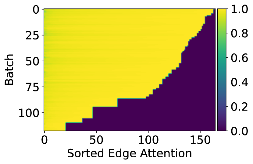
(a) Demo (GSAT)

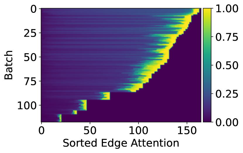
(b) Demo (ours)

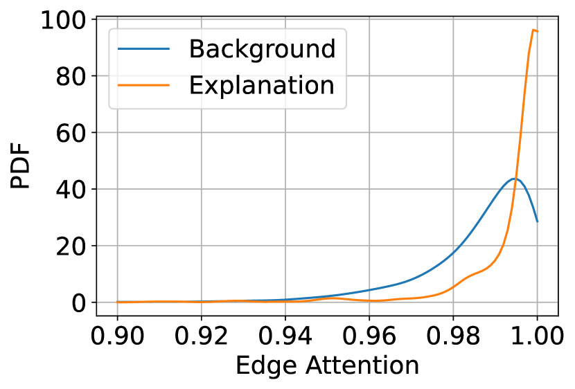
(c) PDF (GSAT)

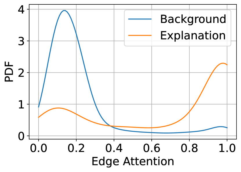
(d) PDF (ours)

Figure 1: Subgraph sparsity of GSAT [26] and our GSINA ($r=0.3$) on a batch of data in SPMotif ($b=0.5$) dataset. Fig. 1(a), 1(b) demonstrate the learned edge importances (attention values) by GSAT and our GSINA for each edge of the graphs in the batch, the bottom right black regions are non-edge padding. The X-axis represents edges (sorted by attention values), and the Y-axis represents graphs. Fig. 1(c), 1(d) are the PDF plots of edge attention distributions generated by GSAT and our GSINA for the edges in Background (label-independent) part and Explanation (label-related) part.

The invariance optimization methods [26; 46; 8] have made considerable efforts for the sound generalizability and inherent interpretability of their invariant feature discovery, and there are two mainstream schemes: 1) the Information Bottleneck (IB) [36] scheme [54; 26] exploits IB principle to extract label-relevant graph invariant features with information constraint, 2) the top-$k$ Subgraph Selection scheme [46; 8] intuitively chooses the top-$k$ most influential edges as the ‘invariant subgraph’. Despite the success of those studies, there are still limitations that need to be stated and addressed for the effectiveness of their methods.

For the IB based methods, they might not proactively guarantee the sparsity of subgraphs, which has also been mentioned in [26]. As shown in Fig. 1, we provide a demonstration with the latest IB based GIL SOTA: Graph Stochastic Attention (GSAT) [26], which evaluates the importance of each edge by assigning edge attention, and as shown in Fig. 1(a), 1(c), GSAT lacks sparsity: the edge attention for the Background part and the Explanation part are similar, making it difficult to make a prediction based on the most valuable invariant features, which are supposed to be more distinguishable.

For the top-$k$ based methods, they capture the invariant subgraph in a ‘hard’ way, i.e. only the top-$k$ part is kept for training and prediction, and the other part is neglected. As only restricted information is utilized, hard subgraph extraction results in a restricted solution space to find the optimal invariant subgraph, and problematically, an ill-posed optimization: the top-$k$ selection operation itself is not differentiable (it does not provide gradients for model backward pass), to make them ‘trainable’, these methods are ‘partially differentiable’ for learning after assigning the differentiable weighting scores output from their subgraph extractors for top-$k$ selection to the extracted subgraph (as the practices in [46; 8]). Moreover, as the top-$k$ selection discards part of the graph structure, these methods could only be used for the tasks of graph level, for a grainer task level, e.g. node level, these methods are not applicable as the graph structure is incomplete (part of the nodes have been discarded), and there is no way to learn all of the node representations.

TABLE I: Comparison with SOTA invariance optimization GIL methods.

	Sparse	Soft	Differentiable
GSAT [26] (IB)	No	Yes	Fully
CIGA [8] (top-$k$)	Yes	No	Partially
Ours	Yes	Yes	Fully

How to extract the invariant subgraph for graph invariant learning? We summarize 3 principles for an invariant subgraph extractor to address the above-mentioned issues of invariance optimization GIL: 1) sparsity (as shown in Fig. 1(b), 1(d)) to effectively filter out the variant features, and the invariant subgraph should be sufficiently distinguishable to avoid confusion with the variant part, 2) softness (compared with the ‘hard selection’ ways) to enlarge the subgraph solution space, to numerically evaluate the graph feature importances, and no graph information omissions, and 3) differentiability (also based on softness) for a soundly end-to-end optimization, and to ensure the invariant subgraph extractor could be learned to generate sparse and soft subgraphs.

To achieve these principles, we have also taken inspiration from the designs and characteristics of the existing GIL works [46; 26; 8], as summarized in Tab. I, GSAT [26] is soft and differentiable as it is based on graph attention mechanism, DIR [46] and CIGA [8] are sparse as their top-$k$ operations explicitly constrain the proportion of their subgraphs to their input graphs. Additionally, recent advances in cardinality-constrained combinatorial optimization [49; 43] illustrate that the top-$k$ problem could be addressed in an approximated soft version by a series of soft and differentiable iterative numerical calculations of the Optimal Transport (OT) [29] theoretic Sinkhorn algorithm [33], with bounded constraint violations. Based on these fundamental endeavors, we propose a novel and general graph attention mechanism [40; 26]: Graph Sinkhorn Attention (GSINA) for improving GIL tasks of multiple levels, GSINA evaluates the graph features (nodes and edges) importance by assigning sparse and soft graph attention values. As an invariance optimization method, GSINA defines its invariant subgraph in the manner of graph attention, which serves as a powerful regularization to improve GIL.

Therefore, our contributions are as follows successively:

1) We analyze the necessity of sparsity, softness, and differentiability in subgraph extraction for GIL, which is lacking in previous IB and top-$k$ based methods.

2) We propose Graph Sinkhorn Attention (GSINA), a GIL framework by learning fully differentiable invariant subgraphs with controllable sparsity and softness to improve multiple levels of graph generalization tasks.

3) Extensive experiments validate the superiority of our GSINA, which could outperform the state-of-the-art GIL methods by large margins.

II Preliminaries and Related Works

The related works cover different aspects of our work, including the problem formulation of graph out-of-distribution (OOD) generalization and Graph Invariant Learning (GIL), the inductive bias behind invariant subgraph extraction, and the cardinality-constrained combinatorial optimization for a fully differentiable top-$k$ operation.

II-A Graph Invariant Learning

The concept of invariant learning involves utilizing the invariant relationships between features and labels across various distributions while disregarding any spurious correlations that may arise [24]. Through this approach, it is possible to attain a high level of out-of-distribution (OOD) generalization in the presence of distribution shifts.

Graph OOD problem considers a series of graph datasets $\mathcal{G}=\{\mathcal{G}^{e}\}_{e}$ collected from multiple environments $\mathcal{E}_{\text{all}}$. For each dataset $\mathcal{G}^{e}=\{(G_{i}^{e},Y_{i}^{e})\}_{i=1}^{N^{e}}$ collected from environment $e$, $(G_{i}^{e},Y_{i}^{e})$ is a graph-label pair sampled from it and $N^{e}$ is the number of such pairs in $\mathcal{G}_{e}$. In the graph OOD settings, the environments of the training and testing datasets, i.e. $\mathcal{E}_{tr}$ and $\mathcal{E}_{te}$ are always different, leading to the problem of distribution shift and the demand for model generalizability. The environment label $e$ for graphs is always unobserved since it is expensive to collect for most scenarios. Therefore, methods that impose requirements on environmental labels also limit their practical application.

Graph Invariant Learning (GIL) is aimed at learning an environment-agnostic function $f:\bigcup\mathcal{G}\rightarrow\mathcal{Y}$ to predict the label $Y$ for downstream tasks. The goal of GIL is to train an optimal $f^{*}$ that it generalizes well on all environments, we can formulate the problem as:

$$f^{*}=\arg\min_{f}\max_{e\in\mathcal{E}_{all}}\mathcal{R}(f|e),$$ (1)

where $\mathcal{R}(f|e)=\mathbb{E}_{(G,Y)\in\mathcal{G}^{e}}[l(f(G),Y)]$ is the empirical risk of the predictor $f$ on the environment $e$ and $l:\mathcal{Y}\times\mathcal{Y}\rightarrow\mathbb{R}$ is the loss function.

As the problem in Eq. 1 is difficult to solve since the environment variable $e$ is always unobserved, a new line of research has emerged recently that focuses on subgraphs, with the goal of identifying an invariant subgraph of the input, which has a stable relationship to the label; and filtering out the other part of the input, which is environment-relevant or spurious. There are existing approaches that aim to explicitly extract invariant subgraphs (with various definitions), guided by the information bottleneck (IB) principle [54; 26] or top-$k$ selection [46; 8]. In particular, [26] introduces Graph Stochastic Attention (GSAT), a novel attention mechanism that constructs inherently interpretable and generalizable GNNs. The attention is formulated as an information bottleneck by introducing stochasticity into the attention mechanism, which constrains the information flow from the input graph to the prediction. By penalizing the amount of information from the input data, GSAT is expected to be more generalizable. [8] proposes a Causality Inspired Invariant Graph LeArning (CIGA) framework to capture the invariance of graphs under various distribution shifts. Specifically, they characterize potential distribution shifts on graphs with causal models, which focus only on subgraphs containing the most information regarding the causes of labels. Overall, these new approaches provide exciting opportunities for achieving interpretability and generalizability in GNNs without requiring expensive domain labels.

II-B Cardinality-Constrained Combinatorial Optimization

Combinatorial optimization (CO) is a fundamental problem of computer science and operations research [3]. Particularly, cardinality-constraint optimization is a permutation-based CO problem that exists widely in real-world applications [7; 6], whose final solution includes at most $k$ non-zero entries, i.e., the cardinality constraint $\|\mathbf{x}\|_{0}\leq k$. Choosing the top-$k$ most influential edges for the invariant subgraph, which is a constraint-critical scenario, could also be regarded as a cardinality-constraint CO problem. Handling the constraint violation is the core of the cardinality-constraint CO problem as a tighter constraint violation leads to better performance [43]. Erdos Goes Neural [19] places a penalty term for a constraint violation in the loss, but the constraint violation is unbounded. [48] develops a soft algorithm by recasting the top-$k$ selection as an optimal transport problem [41] with the Sinkhorn algorithm [33]. Although the upper limit of constraint violation is provided, in the worst situation, the bound might diverge. [43] further addresses the issue and proposes a method with a tighter upper bound by introducing the Gumbel trick, making the constraint violation arbitrarily controlled. These studies provide us with a theoretical basis to formulate the problem of GIL from the perspective of combinatorial optimization.

III Approach

In this section, we first introduce the optimization, or learning objective of our Graph Sinkhorn Attention (GSINA) for Graph Invariant Learning (GIL) at a high level in Sec. III-A. Then in Sec. III-B we present the implementation details of GSINA: the utilization of the Sinkhorn algorithm to obtain the sparse, soft, and differentiable invariant subgraph as a kind of graph attention mechanism, and the general representation learning framework for GIL of multiple-level tasks.

III-A Graph Sinkhorn Attention: Optimization

Aiming at finding the invariant subgraph $G_{S}$ with a stable relationship to the label $Y$, we formulate it as a mutual information $I(G_{S};Y)$ maximization problem like the practices in [54; 26; 8]. On the other hand, constraints should be applied on the invariant subgraph $G_{S}$ to ensure its informative conciseness (i.e., the information of the variant or redundant part of the input graph $G$ should be damped), the constraints act as regularizations and improve the generalization of graph learning tasks. As we discussed in Sec. I, the information bottleneck (IB) based methods [54; 26] might hardly guarantee the subgraph conciseness (lack of sparsity), and the partially differentiable top-$k$ selection based methods [46; 8] generate hard subgraphs and shrink the subgraph solution space. Differently, we leverage a subgraph extractor $g_{\phi}(G,r,\tau)$ generating softly cardinality-constrained subgraph $G_{S}$, the subgraph ratio $r$ is the cardinality constraint controlling the sparsity of $G_{S}$, and $\tau$ is a temperature hyperparameter controlling the softness of $G_{S}$, which will be detailedly discussed in Sec. III-B.

Our subgraph extractor $g_{\phi}(G,r,\tau)$ acts as a sparsity and softness regularization of $G_{S}$, and the mutual information maximization problem can be formulated as:

$$\max_{\phi}I\left(G_{S};Y\right),\,\text{s.t.}\,\,G_{S}\sim g_{\phi}(G,r,\tau).$$ (2)

As the direct estimation of mutual information $I(G_{S};Y)$ is intractable, we derive its lower bound with the help of a variational approximation distribution $P_{\theta}(Y|G_{S})$ parameterized by $\theta$, which also acts as the predictor of label $Y$ given the invariant subgraph $G_{S}$:

$$I\left(G_{S};Y\right)=\iint_{G_{S},Y}P(G_{S},Y)\log\frac{P(G_{S},Y)}{P(G_{S})P(Y)}\mathrm{d}G_{S}\mathrm{d}Y$$ (3)

$$=\int_{G_{S}}P(G_{S})\int_{Y}P(Y|G_{S})\log P_{\theta}(Y|G_{S})\mathrm{d}Y$$

$$\quad+KL[P(Y|G_{S})\|P_{\theta}(Y|G_{S})]\mathrm{d}G_{S}+H(Y)$$

$$\geq\int_{G_{S}}P(G_{S})\int_{Y}P(Y|G_{S})\log P_{\theta}(Y|G_{S})\mathrm{d}Y\mathrm{d}G_{S}+H(Y)$$

$$=\mathbb{E}_{G_{S},Y}\left[\log{P_{\theta}(Y|G_{S})}\right]+H(Y),$$

where $H(Y)=-\int_{Y}P(Y)\log P(Y)\mathrm{d}Y$ is a constant entropy of the label distribution $P(Y)$ and can be omitted in the optimization, the problem in Eq. 2 can be optimized by maximizing the lower bound item in Eq. 3 and the final learning objective of GSINA is:

$$\max_{\theta,\phi}\,\mathbb{E}_{G_{S},Y}\left[\log{P_{\theta}(Y|G_{S})}\right],\,\text{s.t.}\,\,G_{S}\sim g_{\phi}(G,r,\tau).$$ (4)

It results in an end-to-end forward pipeline: first extracting the invariant subgraph $G_{S}$ from the input graph $G$, then making prediction $Y$ based on $G_{S}$. Note that though sharing similarities, GSINA is unlike the IB based methods [54; 26]: the subgraph information of GSINA is constrained by our subgraph extractor $g_{\phi}(G,r,\tau)$, which is able to explicitly control the sparsity $r$ and softness $\tau$ of the invariant subgraph.

III-B Graph Sinkhorn Attention: Implementation

To extract a sparse, soft, and differentiable invariant subgraph $G_{S}$ from the input graph $G$, we leverage a softly cardinality-constrained subgraph extractor $g_{\phi}(G,r,\tau)$ based on the Sinkhorn Algorithm.

The goal of graph attention mechanisms [40; 26] is to assign attention coefficients to different parts of the input graph structure, evaluating their respective importance for the prediction of the target label $Y$. Beyond the graph attention mechanisms designed in [40; 26], we take the sparsity and softness of the attention distribution into consideration by applying differentiable top-$k$ [48; 43] to evaluate the importance of edges. According to Sec. II-B, it has a corresponding popular OT-theoretic solution of the Sinkhorn algorithm [33], and the Gumbel re-parameterization trick could be adopted to enhance the performance according to the practice in [43]. For edge attention, GSINA softly highlights the top-$r$ ratio most influential edges and ‘filters out’ other edges by assigning sparse edge attention to the input graph $G$ (as shown in Fig. 1, 2) and provides soft attention distribution. Based on GSINA edge attention, sparse and soft GSINA node attention could be designed based on graph neighborhood aggregation to evaluate the importance of nodes.

We will start by describing the implementation of edge and node attention in GSINA, and then the general framework for multiple-level GIL tasks via GSINA.

Edge Attention. As an initial step, a composition of $\text{GNN}_{\phi}$ and $\text{MLP}_{\phi}$ is leveraged to obtain learnable node features $\left\{\mathbf{n}_{i}|i\in\mathcal{V}\right\}$ and edge scores $s=\{s_{e}|e\in\mathcal{E}\}$ of the input graph $G=(\mathcal{V},\mathcal{E})$:

$$\left\{\mathbf{n}_{i}\right\} =\text{GNN}_{\phi}(G),\,\,i\in\mathcal{V},$$ (5)

$$s_{e} =\text{MLP}_{\phi}(\mathbf{n}_{i},\mathbf{n}_{j}),\,\,e=(i,j).$$

Softly selecting the top-$r$ scored edges as the invariant subgraph could be interpreted as a relaxed OT problem, whose setting is to move $rN_{e}$ items to the destination of the invariant part, and the other $(1-r)N_{e}$ elements to the other destination of the variant part, where $N_{e}$ is the number of the edges. During the training phase, the Gumbel re-parameterization trick $\tilde{s_{e}}=s_{e}-\sigma\log(-\log u_{e}),u_{e}\sim U(0,1)$ [17; 43], where $\sigma$ is the factor of Gumbel noise and $\sigma=0$ in validation and testing phases, could be adopted to enlarge the sampling space and to improve the generalization performances, i.e. the Gumbel trick allows less important edges to participate in training (without being poorly trained due to low attention, resulting in underfitting), and remains the sampling accuracy. Defining $\mathbf{D}$ as the distance matrix of the OT problem, $\mathbf{R}$ and $\mathbf{C}$ as the marginal distributions, and $\mathbf{T}$ as the transportation plan moving $rN_{e}$ items to $\text{max}(s)$ (invariant) and $(1-r)N_{e}$ items to $\text{min}(s)$ (variant), the OT problem for GSINA edge attention can be formulated as follows:

$$\begin{gathered}\mathbf{D}=\begin{bmatrix}\tilde{s_{1}}-\min(s),&\tilde{s_{2}}-\min(s),&\dots,&\tilde{s}_{N_{e}}-\min(s)\\ \max(s)-\tilde{s_{1}},&\max(s)-\tilde{s_{2}},&\dots,&\max(s)-\tilde{s}_{N_{e}}\end{bmatrix},\\ \mathbf{R}=[(1-r)N_{e},\,rN_{e}]^{\top},\,\mathbf{C}=[1,\,1,\,\dots,\,1]^{\top}\in\mathbb{R}^{N_{e}\times 1},\\ \min_{\mathbf{T}}\text{tr}(\mathbf{T}^{\top}\mathbf{D})-\tau H(\mathbf{T}),\\ \text{s.t.}\quad\mathbf{T}\in[0,1]^{2\times N_{e}},\,\,\mathbf{T}\mathbf{1}=\mathbf{R},\,\,\mathbf{T}^{\top}\mathbf{1}=\mathbf{C},\end{gathered}$$ (6)

where $\tau H(\mathbf{T})$ is the entropic regularizer [12] of the OT problem, and $\tau$ is the temperature hyperparameter controlling the softness of the transportation plan $\mathbf{T}$. The result of $\mathbf{T}$ could be iteratively calculated by the Sinkhorn algorithm:

$$\mathbf{T}_{0}=\exp\left(-\frac{\mathbf{D}}{\tau}\right),$$ (7)

$$\mathbf{T}_{k}=\operatorname{diag}\left(\mathbf{T}_{k-1}\mathbf{1}\oslash\mathbf{R}\right)^{-1}\mathbf{T}_{k-1},$$ (8)

$$\mathbf{T}_{k}=\mathbf{T}_{k-1}\operatorname{diag}(\mathbf{T}_{k-1}^{\top}\mathbf{1}\oslash\mathbf{C})^{-1},$$ (9)

where $\mathbf{T}_{0}$ in Eq. 7 is the initialization, the equations of $\mathbf{T}_{k}$ in Eq. 8 and 9 are alternative iterations of row- and column-wise normalizations to satisfy the two constraints $\mathbf{T}\mathbf{1}=\mathbf{R}$ and $\mathbf{T}^{\top}\mathbf{1}=\mathbf{C}$, $\oslash$ is element-wise division.

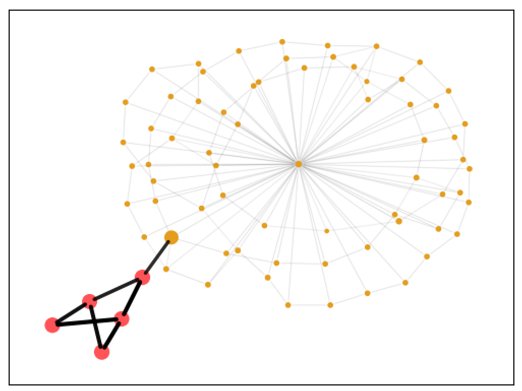
Figure 2: Example of GSINA invariant subgraph $G_{S}$ from SPMotif dataset. The ground truth (nodes) of the invariant subgraph is colored red, and the other part is yellow. The edge widths and node sizes are given by GSINA original outputs (we do not apply sharpening tricks for visualizations like GSAT [26] and CIGA [9]). It is shown that our GSINA assigns sparse and soft attention $\{\alpha^{V},\alpha^{E}\}$ to the nodes and edges of the input graph $G$. More visualization results can be found in https://github.com/dingfangyu/GSINA/vis.

Eventually, the edge attention $\alpha^{E}=\{\alpha^{E}_{e}|e\in\mathcal{E}\}$ could be obtained from the procedure above:

$$\left[\alpha^{E}_{1},\,\alpha^{E}_{2},\,\dots,\alpha^{E}_{N_{e}}\right]=\mathbf{T}[1,:].$$ (10)

Node Attention. Given the sparse, soft, and differentiable edge attention $\alpha^{E}$, a natural consideration is to evaluate the importance of nodes. Hence, the node attention $\alpha^{V}=\{\alpha^{V}_{i}|i\in\mathcal{V}\}$ in our GSINA is proposed, which could be obtained by an aggregation of the edge attention in the neighborhood of each node $i$:

$$\alpha^{V}_{i}=\text{AGG}(\{\alpha^{E}_{e}|e=(i,j)\land e\in\mathcal{E}\}).$$ (11)

For the ‘hard’ top-$k$ based GIL methods [46; 8], only the selected part is kept to be the invariant subgraph $G_{S}$ and the other part $\overline{G_{S}}$ is just discarded. In other words, the node importance is 1 for nodes in $G_{S}$ and 0 for nodes in $\overline{G_{S}}$. Our node attention is a soft and fully differentiable version to mimic their invariant subgraph extractions.

General Graph Invariant Learning Framework. Our invariant subgraph extraction results in a graph weighted by the Graph Sinkhorn (Edge and Node) Attention, with the properties of sparsity, softness, and differentiability, the mathematical definition of the invariant subgraph $G_{S}$ of our GSINA is in the manner of graph attention:

$$G_{S}=\{G,\alpha^{V},\alpha^{E}\}\sim g_{\phi}(G,r,\tau).$$ (12)

Based on the definition of our invariant subgraph in Eq. 12, the prediction process (the predictor $P_{\theta}(Y|G_{S})$ in Eq. 4) could be regularized by our GSINA message passing mechanism in Eq. 13. For the $l$-th GNN message passing layer, GSINA weights each message $m_{\theta}(\mathbf{h}_{i}^{(l)},\mathbf{h}_{j}^{(l)},\mathbf{h}_{ij}^{(l)})$ by edge attention $\alpha^{E}_{ij}$, $\mathbf{h}_{ij}^{(l)}$ is the representation of edge $(i,j)$ (if applicable), $\bigoplus$ is any permutation invariant aggregation function, $\gamma_{\theta}$ is the GNN update function, and $\mathbf{h}_{i}^{(l+1)}$ is updated representation. If the graph representation $\mathbf{h}_{G}$ is obtained from a readout $f_{\theta}$ of node representations output from the $L$-th (final) GNN layer $\{\mathbf{h}_{i}^{(L)}|i\in\mathcal{V}\}$, each node representation $\mathbf{h}_{i}^{(L)}$ is weighted by our node attention $\alpha^{V}_{i}$ in our GSINA, GSINA is general due to its applicability to multiple-level (i.e. graph-level and node-level) GIL tasks:

$$\mathbf{h}_{i}^{(l+1)} =\gamma_{\theta}\left(\mathbf{h}_{i}^{(l)},\bigoplus_{j\in\mathcal{N}_{i}}\alpha^{E}_{ij}*m_{\theta}(\mathbf{h}_{i}^{(l)},\mathbf{h}_{j}^{(l)},\mathbf{h}_{ij}^{(l)})\right),$$ (13)

$$\mathbf{h}_{G}\,\,\,\, =f_{\theta}\left(\{\alpha^{V}_{i}*\mathbf{h}_{i}^{(L)}|i\in\mathcal{V}\}\right).$$ (14)

The procedure of the GSINA training algorithm is shown in Alg. 1.

Algorithm 1 The training procedure.

Parameters: the number of training epoch $E$; the number of batch size $B$; the sparsity $r$; the softness $\tau$; the sinkhorn iterations $n$.

Input: training dataset $\mathcal{G}=\{G_{i},Y_{i}\}_{i}^{N}$.

Output: the trained parameters $\theta$ and $\phi$ in Sec. III-A.

1:  Initialize parameters $\theta$ and $\phi$;// For each epoch

2:  for $i=1,\dots,E$ do

3:     Sample data batches $\mathcal{B}=\{\mathcal{G}_{1},\mathcal{G}_{2},\dots,\mathcal{G}_{b}\}$ from $\mathcal{G}$ with batch size $B$;// For each batch

4:     for $j=1,\dots,b$ do

5:        $G=\{G_{m}|(G_{m},Y_{m})\in\mathcal{G}_{j}\}$;

6:        $Y=\{Y_{m}|(G_{m},Y_{m})\in\mathcal{G}_{j}\}$;// Forward: get $G_{S}=\{G,\alpha^{V},\alpha^{E}\}\sim g_{\phi}(G,r,\tau)$ by Eq. 12

7:        Get edge scores $s=\{s_{e}|e\in\mathcal{E}\}$ with $\text{GNN}_{\phi}$ and $\text{MLP}_{\phi}$ by Eq. 5;

8:        Prepare $\mathbf{D},\mathbf{R},\mathbf{C}$ of the OT problem by Eq. 6;

9:        Initialize $\mathbf{T}_{0}$ by Eq. 7;

10:        for $k=1,\dots,n$ do

11:           Update $\mathbf{T}_{k}$ by Eq. 8 and 9;

12:        end for

13:        Get GSINA edge and node attention $\{\alpha^{V},\alpha^{E}\}$ by Eq. 10 and 11; // Forward: get the learning objective $\log{P_{\theta}(Y|G_{S})}$ in Eq. 4 by Eq. 13 and 14

14:        if Graph-level GIL task then

15:           Get $h_{G}$ by Eq. 14;

16:           Modelize the distribution $P_{\theta}(Y|G_{S})$ with $h_{G}$;

17:        else if Node-level GIL task then

18:           Get $\{h^{L}_{v}|v\in\mathcal{V}\}$ by Eq. 13;

19:           Modelize the distribution $P_{\theta}(Y|G_{S})$ with $\{h^{L}_{v}|v\in\mathcal{V}\}$;

20:        end if

21:        Get the learning objective $\log{P_{\theta}(Y|G_{S})}$ in Eq. 4; // Backward

22:        Optimize parameters $\theta$ and $\phi$ via gradient descent;

23:     end for

24:  end for

25:  Output the parameters $\theta$ and $\phi$;

IV Experiments

To demonstrate our GSINA’s superiority, we conduct experiments on various graph invariant learning tasks, including graph-level and node-level OOD generalizations. For the graph-level GIL, we compare with both IB and top-$k$ based SOTAs, i.e. GSAT [26] and CIGA [8], respectively. It is worth noting the reason for performing separate experiments is for fair comparisons, as the experimental settings of these two benchmarks of GSAT and CIGA are quite different, including differences in datasets, GNN backbones, baselines, etc. Besides, both GSAT and CIGA involve extensive hyperparameter tuning, all these present challenges in unifying the benchmarks. Nevertheless, our separate experiments have demonstrated our superiority over each of them. For the node-level GIL, we make a comparison with EERM [45]. Furthermore, we provide 1) hyperparameter studies, 2) ablation studies of GSINA components, 3) runtime and complexity analysis, and 4) interpretability analysis of the extracted invariant subgraph. We introduce the datasets, baselines, evaluation metrics, and experiment settings and provide results analysis in this section. All experiments are conducted for 5 runs on RTX-2080Ti (11GB) GPUs, and the average and standard deviation are reported.

IV-A On Graph-Level Tasks: versus IB Based GIL

TABLE II: Dataset Statistics of the GSAT benchmark used in Tab. LABEL:tab:gsat, following the datasets used in DIR [46].

	Spurious-Motif			MNIST-75sp (reduced)			Graph-SST2			OGBG-Molhiv
	Train	Val	Test	Train	Val	Test	Train	Val	Test	Train	Val	Test
Classes#		3			10			2			2
Graphs#	9,000	3,000	6,000	20,000	5,000	10,000	28,327	3,147	12,305	32,901	4,113	4,113
Avg. N#	25.4	26.1	88.7	66.8	67.3	67.0	17.7	17.3	3.45	25.3	27.79	25.3
Avg. E#	35.4	36.2	131.1	539.3	545.9	540.4	33.3	33.5	4.89	54.1	61.1	55.6
Metrics		ACC			ACC			ACC			ROC-AUC

TABLE III: Comparision with the IB based GIL, graph-level OOD generalization performances on GSAT [26] benchmark.

	MolHiv (AUC)	Graph-SST2	MNIST-75sp	Spurious-motif
				$b=0.5$	$b=0.7$	$b=0.9$
GIB [54]	${76.43}{\scriptstyle\pm 2.65}$	$82.99{\scriptstyle\pm 0.67}$	$93.10{\scriptstyle\pm 1.32}$	$54.36{\scriptstyle\pm 7.09}$	$48.51{\scriptstyle\pm 5.76}$	$46.19{\scriptstyle\pm 5.63}$
DIR [46]	$76.34{\scriptstyle\pm 1.01}$	$82.32{\scriptstyle\pm 0.85}$	$88.51{\scriptstyle\pm 2.57}$	$45.49{\scriptstyle\pm 3.81}$	$41.13{\scriptstyle\pm 2.62}$	$37.61{\scriptstyle\pm 2.02}$
GIN [50]	$76.69{\scriptstyle\pm 1.25}$	$82.73{\scriptstyle\pm 0.77}$	$95.74{\scriptstyle\pm 0.36}$	$39.87{\scriptstyle\pm 1.30}$	$39.04{\scriptstyle\pm 1.62}$	$38.57{\scriptstyle\pm 2.31}$
GIN+GSAT [26]	$76.47{\scriptstyle\pm 1.53}$	$82.95{\scriptstyle\pm 0.58}$	$96.24{\scriptstyle\pm 0.17}$	$52.74{\scriptstyle\pm 4.08}$	$49.12{\scriptstyle\pm 3.29}$	$44.22{\scriptstyle\pm 5.57}$
GIN+ours	$\mathbf{77.99}{\scriptstyle\pm 0.97}$	$\mathbf{83.66}{\scriptstyle\pm 0.37}$	$\mathbf{96.73}{\scriptstyle\pm 0.16}$	$\mathbf{55.16}{\scriptstyle\pm 5.69}$	$\mathbf{56.83}{\scriptstyle\pm 6.32}$	$\mathbf{49.86}{\scriptstyle\pm 6.10}$
PNA [10]	$78.91{\scriptstyle\pm 1.04}$	$79.87{\scriptstyle\pm 1.02}$	$87.20{\scriptstyle\pm 5.61}$	$68.15{\scriptstyle\pm 2.39}$	$66.35{\scriptstyle\pm 3.34}$	$61.40{\scriptstyle\pm 3.56}$
PNA+GSAT [26]	$80.24{\scriptstyle\pm 0.73}$	$80.92{\scriptstyle\pm 0.66}$	$93.96{\scriptstyle\pm 0.92}$	$68.74{\scriptstyle\pm 2.24}$	$64.38{\scriptstyle\pm 3.20}$	$57.01{\scriptstyle\pm 2.95}$
PNA+ours	$\mathbf{80.55}{\scriptstyle\pm 0.97}$	$\mathbf{82.18}{\scriptstyle\pm 1.01}$	$\mathbf{95.48}{\scriptstyle\pm 0.37}$	$\mathbf{76.39}{\scriptstyle\pm 1.85}$	$\mathbf{73.96}{\scriptstyle\pm 2.87}$	$\mathbf{62.51}{\scriptstyle\pm 5.86}$

TABLE IV: Statistics of ogbg-mol* datasets of GSAT benchmark in Tab. LABEL:tab:gsat_ogbg. For all the datasets, we use the scaffold split with the split ratio of 80/10/10.

Name	#Graphs	Average	Average	#Tasks	Task	Metric
		#Nodes	#Edges		Type
bace	1,513	34.1	36.9	1	Binary class.	ROC-AUC
bbbp	2,039	24.1	26.0	1	Binary class.	ROC-AUC
clintox	1,477	26.2	27.9	2	Binary class.	ROC-AUC
tox21	7,831	18.6	19.3	12	Binary class.	ROC-AUC
sider	1,427	33.6	35.4	27	Binary class.	ROC-AUC

TABLE V: Comparision with the IB based GIL, graph-level OOD generalization performances on other OGBG-Mol datasets in GSAT [26] benchmark.

	molbace	molbbbp	molclintox	moltox21	molsider
PNA [10]	$73.52{\scriptstyle\pm 3.02}$	$67.21{\scriptstyle\pm 1.34}$	$86.72{\scriptstyle\pm 2.33}$	$75.08{\scriptstyle\pm 0.64}$	$56.51{\scriptstyle\pm 1.90}$
GSAT [26]	${77.41}{\scriptstyle\pm 2.42}$	$\mathbf{69.17}{\scriptstyle\pm 1.12}$	${87.80}{\scriptstyle\pm 2.36}$	$74.96{\scriptstyle\pm 0.66}$	${57.58}{\scriptstyle\pm 1.23}$
ours	$\mathbf{79.57}{\scriptstyle\pm 1.38}$	$67.86{\scriptstyle\pm 0.91}$	$\mathbf{90.08}{\scriptstyle\pm 2.06}$	$\mathbf{75.47}{\scriptstyle\pm 0.55}$	$\mathbf{58.61}{\scriptstyle\pm 1.09}$

To make a direct and fair comparison with the IB based GIL methods, we choose GSAT [26] as the baseline, we perform evaluations strictly in line with its original experiment settings, including the datasets, GNN backbones, metrics, and optimization settings. To compare with GSAT, the hyperparameter $r$ for GSINA is chosen according to our validation performances. The statistics and evaluation metrics of these datasets are shown in Tab. II and IV and the experiment results are given in Tab. LABEL:tab:gsat, LABEL:tab:gsat_ogbg.

Datasets. We use the synthetic Spurious-Motif (SPMotif) datasets from DIR [46], where each graph is constructed by a combination of a motif graph directly determining the graph label, and a base graph providing spurious correlation to graph label, and we use datasets with spurious correlation degree $b=$ 0.5, 0.7 and 0.9. For real-world datasets, we use MNIST-75sp [21], where each image in MNIST is converted to a superpixel graph, Graph-SST2 [34; 55], which is a sentiment analysis dataset, and each text sequence in SST2 is converted to a graph, following the splits in DIR [46], Graph-SST2 contains degree shifts, and molecular property prediction datasets from the OGBG [47; 15] benchmark (molhiv, molbace, molbbbp, molclintox, moltox21, molsider).

Metrics. We test the classification accuracy (ACC) for SPMotif datasets, MNIST-75sp, Graph-SST2, and ROC-AUC for OGBG datasets following [26].

Baselines. Following the baselines and the corresponding settings in GSAT [26], we compare with interpretable GNNs GIB [54] and DIR [46], and we use GIN [50] and PNA [10] as backbones for GSAT and GSINA.

GNN Backbone Architectures. For GSINA with GIN and PNA backbones for the experiments on GSAT benchmark (reported in Tab. LABEL:tab:gsat, LABEL:tab:gsat_ogbg), our GNN backbone settings of GIN and PNA are strictly in line with those in GSAT settings. We use 2 layers GIN with 64 hidden dimensions and 0.3 dropout ratio. We use 4 layers PNA with 80 hidden dimensions, 0.3 dropout ratio, and no scalars are used. We directly follow PNA and GSAT using (mean, min, max, std) aggregators for OGBG datasets, and (mean, min, max, std, sum) aggregators for all other datasets.

More Architecture Settings. For all experiments of GSINA and for simplicity, the $\text{MLP}_{\phi}$ in our subgraph extractor $g_{\phi}$ is a 2-layer MLP, $\text{MLP}_{\phi}(\mathbf{n}_{i},\mathbf{n}_{j})$ is implemented by inputting concatenated $[\mathbf{n}_{i},\mathbf{n}_{j}]$, and outputting a 1-dim edge score $s_{ij}$, then a batch normalization layer ($s:=\frac{s-\text{mean}(s)}{\text{std}(s)}$) is applied to normalize the edge scores to a stable value range; and the aggregator of GSINA node attention to aggregate the edge attention values in a node’s neighborhood is the ‘max’ aggregator.

Batch Size. In line with GSAT, we use a batch size of 128 for all datasets.

Optimization. We use Adam optimizers for graph classification experiments reported in Tab. LABEL:tab:gsat, LABEL:tab:gsat_ogbg strictly in line with the settings of GSAT. Our GSINA with GIN backbone uses 0.003 learning rate for Spurious-Motifs and 0.001 for all other datasets. Our GSINA with PNA backbone uses 0.003 learning rate for Graph-SST2 and Spurious-Motifs, and 0.001 learning rate for all other datasets.

Epoch. For graph classification experiments on GSAT and CIGA benchmarks, we perform early stopping to avoid overfitting. Based on the difficulty of fitting the dataset, we set the early stopping patience to 10 for the SPMotif (both GSAT and CIGA benchmarks) datasets, DrugOOD-Size and TU datasets, 3 for Graph-SST2 and Graph-SST5, 5 for Twitter, 20 for DrugOOD-Assay/Scaffold and 30 for MNIST-75sp. We do not use early stopping for OGBG datasets (molhiv, molbace, molbbbp, molclintox, moltox21, molsider), and simply train them to the end of epochs (200 epochs for GIN + GSINA, 100 for PNA + GSINA) to achieve better performances. For TU datasets, like the practices of pre-training in CIGA, we pretrain them for 30 epochs to avoid underfitting. For EERM benchmark, we do not perform early stoppings or pre-trainings, we follow the epochs used in EERM work and train to the end, which is 200 epochs for all datasets except for 500 epochs for OGB-Arxiv.

Hyperparameter Settings of $r$. We perform $r$ selection based on the validation performances. For GIN backboned GSINA, we set $r=$ 0.9 for OGBG-Molhiv, 0.2 for Graph-SST2, 0.5 for MNIST-75sp, 0.6 for SPMotif-0.5, 0.6 for SPMotif-0.7, and 0.4 for SPMotif-0.9. For PNA backboned GSINA, we set $r=$ 0.7 for OGBG-Molhiv, 0.5 for OGBG-Molbace, 0.8 for OGBG-Molbbbp, 0.7 for OGBG-Molclintox, 0.7 for OGBG-Moltox21, 0.8 for OGBG-Molsider, 0.8 for Graph-SST2, 0.6 for MNIST-75sp, 0.1 for SPMotif-0.5, 0.3 for SPMotif-0.7, and 0.5 for SPMotif-0.9.

Performances Analysis. Tab. LABEL:tab:gsat reports the graph classification performances on GSAT benchmark, GSINA achieves better performances than the baselines of interpretable GNNs GIB, DIR, and GSAT. GSINA outperforms GSAT by large margins on all 6 datasets for both GNN backbones GIN and PNA. Tab. LABEL:tab:gsat_ogbg reports the graph classification performances for another 5 OGBG-Mol datasets with smaller sizes than those in Tab. LABEL:tab:gsat. Following GSAT, we compare with PNA backboned baselines, and GSINA mostly outperforms.

These improvements demonstrate the effectiveness of our sparsity compared with GSAT (based on IB constraint). Especially, we observe relatively big improvements on SPMotif datasets. There are about at most 10% improvements than GSAT in classification accuracy on SPMotif ($b=0.7$) in Tab. LABEL:tab:gsat, which indicates the superiority of our GSINA on the datasets with more distinguishable subgraph properties, such as the SPMotif datasets, where the invariant subgraphs can be clearly separable due to their data generation processes.

IV-B On Graph-Level Tasks: versus Top-$k$ Based GIL

To make a comparison with the top-$k$ based GIL methods, we choose CIGA [8] as the baseline. The statistics and evaluation metrics of these datasets are shown in Tab. VI and the experiment results are given in Tab. VII, VIII.

TABLE VI: Dataset statistics of CIGA benchmark used in experiments of Tab. VII and VIII.

Datasets	# Training	# Validation	# Testing	# Classes	# Nodes	# Edges	Metrics
SPMotif	$9,000$	$3,000$	$3,000$	$3$	$44.96$	$65.67$	ACC
SST5	$6,090$	$1,186$	$2,240$	$5$	$19.85$	$37.70$	ACC
Twitter	$3,238$	$694$	$1,509$	$3$	$21.10$	$40.20$	ACC
DrugOOD-Assay	$34,179$	$19,028$	$19,032$	$2$	$32.27$	$70.25$	ROC-AUC
DrugOOD-Scaffold	$21,519$	$19,041$	$19,048$	$2$	$29.95$	$64.86$	ROC-AUC
DrugOOD-Size	$36,597$	$17,660$	$16,415$	$2$	$30.73$	$66.90$	ROC-AUC
PROTEINS	$511$	$56$	$112$	$2$	$39.06$	$145.63$	MCC
DD	$533$	$59$	$118$	2	$284.32$	$1,431.32$	MCC
NCI1	$1,942$	$215$	$412$	$2$	$29.87$	$64.6$	MCC
NCI109	$1,872$	$207$	$421$	$2$	$29.68$	$64.26$	MCC

TABLE VII: Comparision with top-$k$ based GIL, graph-level OOD generalization on synthetic datasets of CIGA benchmark.

	SPMotif-Struc			SPMotif-Mixed
	bias=$0.33$	bias=$0.60$	bias=$0.90$	bias=$0.33$	bias=$0.60$	bias=$0.90$
ERM [38]	$59.49{\scriptstyle\pm 3.50}$	$55.48{\scriptstyle\pm 4.84}$	$49.64{\scriptstyle\pm 4.63}$	$58.18{\scriptstyle\pm 4.30}$	$49.29{\scriptstyle\pm 8.17}$	$41.36{\scriptstyle\pm 3.29}$
IRM [2]	$57.15{\scriptstyle\pm 3.98}$	$61.74{\scriptstyle\pm 1.32}$	$45.68{\scriptstyle\pm 4.88}$	$58.20{\scriptstyle\pm 1.97}$	$49.29{\scriptstyle\pm 3.67}$	$40.73{\scriptstyle\pm 1.93}$
V-Rex [22]	$54.64{\scriptstyle\pm 3.05}$	$53.60{\scriptstyle\pm 3.74}$	$48.86{\scriptstyle\pm 9.69}$	$57.82{\scriptstyle\pm 5.93}$	$48.25{\scriptstyle\pm 2.79}$	$43.27{\scriptstyle\pm 1.32}$
EIIL [11]	$56.48{\scriptstyle\pm 2.56}$	$60.07{\scriptstyle\pm 4.47}$	$55.79{\scriptstyle\pm 6.54}$	$53.91{\scriptstyle\pm 3.15}$	$48.41{\scriptstyle\pm 5.53}$	$41.75{\scriptstyle\pm 4.97}$
IB-IRM [1]	$58.30{\scriptstyle\pm 6.37}$	$54.37{\scriptstyle\pm 7.35}$	$45.14{\scriptstyle\pm 4.07}$	$57.70{\scriptstyle\pm 2.11}$	$50.83{\scriptstyle\pm 1.51}$	$40.27{\scriptstyle\pm 3.68}$
CNC [56]	$70.44{\scriptstyle\pm 2.55}$	$66.79{\scriptstyle\pm 9.42}$	$50.25{\scriptstyle\pm 10.7}$	$65.75{\scriptstyle\pm 4.35}$	$59.27{\scriptstyle\pm 5.29}$	$41.58{\scriptstyle\pm 1.90}$
ASAP [30]	$64.87{\scriptstyle\pm 13.8}$	$64.85{\scriptstyle\pm 10.6}$	$57.29{\scriptstyle\pm 14.5}$	$66.88{\scriptstyle\pm 15.0}$	$59.78{\scriptstyle\pm 6.78}$	$50.45{\scriptstyle\pm 4.90}$
DIR [46]	$58.73{\scriptstyle\pm 11.9}$	$48.72{\scriptstyle\pm 14.8}$	$41.90{\scriptstyle\pm 9.39}$	$67.28{\scriptstyle\pm 4.06}$	$51.66{\scriptstyle\pm 14.1}$	$38.58{\scriptstyle\pm 5.88}$
CIGAv1 [8]	$71.07{\scriptstyle\pm 3.60}$	$63.23{\scriptstyle\pm 9.61}$	$51.78{\scriptstyle\pm 7.29}$	$74.35{\scriptstyle\pm 1.85}$	$64.54{\scriptstyle\pm 8.19}$	$49.01{\scriptstyle\pm 9.92}$
CIGAv2 [8]	$\mathbf{77.33}{\scriptstyle\pm 9.13}$	$69.29{\scriptstyle\pm 3.06}$	$63.41{\scriptstyle\pm 7.38}$	$72.42{\scriptstyle\pm 4.80}$	$70.83{\scriptstyle\pm 7.54}$	$54.25{\scriptstyle\pm 5.38}$
ours	$75.49{\scriptstyle\pm 4.26}$	$\mathbf{74.25}{\scriptstyle\pm 2.53}$	$\mathbf{73.54}{\scriptstyle\pm 5.54}$	$\mathbf{82.70}{\scriptstyle\pm 6.28}$	$\mathbf{77.03}{\scriptstyle\pm 2.66}$	$\mathbf{68.89}{\scriptstyle\pm 8.17}$
Oracle (IID)	$88.70{\scriptstyle\pm 0.17}$	$88.70{\scriptstyle\pm 0.17}$	$88.70{\scriptstyle\pm 0.17}$	$88.73{\scriptstyle\pm 0.25}$	$88.73{\scriptstyle\pm 0.25}$	$88.73{\scriptstyle\pm 0.25}$

TABLE VIII: Comparision with top-$k$ based GIL, graph-level OOD generalization on real-world datasets of CIGA [8] benchmark, bold font for the best performance on each dataset and underline for the second.

	Graph-SST5	Twitter	Drug-Assay	Drug-Sca	Drug-Size	NCI1	NCI109	PROT	DD
ERM [38]	$43.89{\scriptstyle\pm 1.73}$	$60.81{\scriptstyle\pm 2.05}$	$71.79{\scriptstyle\pm 0.27}$	$68.85{\scriptstyle\pm 0.62}$	$66.70{\scriptstyle\pm 1.08}$	$0.15{\scriptstyle\pm 0.05}$	$0.16{\scriptstyle\pm 0.02}$	$0.22{\scriptstyle\pm 0.09}$	$0.27{\scriptstyle\pm 0.09}$
IRM [2]	$43.69{\scriptstyle\pm 1.26}$	$63.50{\scriptstyle\pm 1.23}$	$72.12{\scriptstyle\pm 0.49}$	$68.69{\scriptstyle\pm 0.65}$	$66.54{\scriptstyle\pm 0.42}$	$0.17{\scriptstyle\pm 0.02}$	$0.14{\scriptstyle\pm 0.01}$	$0.21{\scriptstyle\pm 0.09}$	$0.22{\scriptstyle\pm 0.08}$
V-Rex [22]	$43.28{\scriptstyle\pm 0.52}$	$63.21{\scriptstyle\pm 1.57}$	$72.05{\scriptstyle\pm 1.25}$	$68.92{\scriptstyle\pm 0.98}$	$66.33{\scriptstyle\pm 0.74}$	$0.15{\scriptstyle\pm 0.04}$	$0.15{\scriptstyle\pm 0.04}$	$0.22{\scriptstyle\pm 0.06}$	$0.21{\scriptstyle\pm 0.07}$
EIIL [11]	$42.98{\scriptstyle\pm 1.03}$	$62.76{\scriptstyle\pm 1.72}$	$72.60{\scriptstyle\pm 0.47}$	$68.45{\scriptstyle\pm 0.53}$	$66.38{\scriptstyle\pm 0.66}$	$0.14{\scriptstyle\pm 0.03}$	$0.16{\scriptstyle\pm 0.02}$	$0.20{\scriptstyle\pm 0.05}$	$0.23{\scriptstyle\pm 0.10}$
IB-IRM [1]	$40.85{\scriptstyle\pm 2.08}$	$61.26{\scriptstyle\pm 1.20}$	$72.50{\scriptstyle\pm 0.49}$	$68.50{\scriptstyle\pm 0.40}$	$66.64{\scriptstyle\pm 0.28}$	$0.12{\scriptstyle\pm 0.04}$	$0.15{\scriptstyle\pm 0.06}$	$0.21{\scriptstyle\pm 0.06}$	$0.15{\scriptstyle\pm 0.13}$
CNC [56]	$42.78{\scriptstyle\pm 1.53}$	$61.03{\scriptstyle\pm 2.49}$	$72.40{\scriptstyle\pm 0.46}$	$67.24{\scriptstyle\pm 0.90}$	$65.79{\scriptstyle\pm 0.80}$	$0.16{\scriptstyle\pm 0.04}$	$0.16{\scriptstyle\pm 0.04}$	$0.19{\scriptstyle\pm 0.08}$	$0.27{\scriptstyle\pm 0.13}$
ASAP [30]	$44.16{\scriptstyle\pm 1.36}$	$60.68{\scriptstyle\pm 2.10}$	$70.51{\scriptstyle\pm 1.93}$	$66.19{\scriptstyle\pm 0.94}$	$64.12{\scriptstyle\pm 0.67}$	$0.16{\scriptstyle\pm 0.10}$	$0.15{\scriptstyle\pm 0.07}$	$0.22{\scriptstyle\pm 0.16}$	$0.21{\scriptstyle\pm 0.08}$
GIB [54]	$38.64{\scriptstyle\pm 4.52}$	$48.08{\scriptstyle\pm 2.27}$	$63.01{\scriptstyle\pm 1.16}$	$62.01{\scriptstyle\pm 1.41}$	$55.50{\scriptstyle\pm 1.42}$	$0.13{\scriptstyle\pm 0.10}$	$0.16{\scriptstyle\pm 0.02}$	$0.19{\scriptstyle\pm 0.08}$	$0.01{\scriptstyle\pm 0.18}$
DIR [46]	$41.12{\scriptstyle\pm 1.96}$	$59.85{\scriptstyle\pm 2.98}$	$68.25{\scriptstyle\pm 1.40}$	$63.91{\scriptstyle\pm 1.36}$	$60.40{\scriptstyle\pm 1.42}$	$0.21{\scriptstyle\pm 0.06}$	$0.13{\scriptstyle\pm 0.05}$	$0.25{\scriptstyle\pm 0.14}$	$0.20{\scriptstyle\pm 0.10}$
CIGAv1 [8]	$44.71{\scriptstyle\pm 1.14}$	$63.66{\scriptstyle\pm 0.84}$	${72.71}{\scriptstyle\pm 0.52}$	$69.04{\scriptstyle\pm 0.86}$	$67.24{\scriptstyle\pm 0.88}$	${0.22}{\scriptstyle\pm 0.07}$	$\mathbf{0.23}{\scriptstyle\pm 0.09}$	$\underline{0.40}{\scriptstyle\pm 0.06}$	$\mathbf{0.29}{\scriptstyle\pm 0.08}$
CIGAv2 [8]	$\underline{45.25}{\scriptstyle\pm 1.27}$	$\underline{64.45}{\scriptstyle\pm 1.99}$	$\mathbf{73.17}{\scriptstyle\pm 0.39}$	$\mathbf{69.70}{\scriptstyle\pm 0.27}$	$\mathbf{67.78}{\scriptstyle\pm 0.76}$	$\underline{0.27}{\scriptstyle\pm 0.07}$	$\underline{0.22}{\scriptstyle\pm 0.05}$	$0.31{\scriptstyle\pm 0.12}$	$0.26{\scriptstyle\pm 0.08}$
ours	$\mathbf{45.84}{\scriptstyle\pm 0.52}$	$\mathbf{64.64}{\scriptstyle\pm 1.71}$	$\underline{72.84}{\scriptstyle\pm 0.50}$	$\underline{69.57}{\scriptstyle\pm 0.39}$	$\underline{67.48}{\scriptstyle\pm 0.33}$	$\mathbf{0.28}{\scriptstyle\pm 0.07}$	${0.21}{\scriptstyle\pm 0.04}$	$\mathbf{0.41}{\scriptstyle\pm 0.07}$	$\mathbf{0.29}{\scriptstyle\pm 0.07}$
Oracle (IID)	$48.18{\scriptstyle\pm 1.00}$	$64.21{\scriptstyle\pm 1.77}$	$85.56{\scriptstyle\pm 1.44}$	$84.71{\scriptstyle\pm 1.60}$	$85.83{\scriptstyle\pm 1.31}$	$0.32{\scriptstyle\pm 0.05}$	$0.37{\scriptstyle\pm 0.06}$	$0.39{\scriptstyle\pm 0.09}$	$0.33{\scriptstyle\pm 0.05}$

Datasets. We use the synthetic SPMotif datasets from DIR, with structural shift degrees $b=$ 0.33, 0.6 and 0.9, denoted as SPMotif (-struc). Besides, we use the SPMotif (-mixed) from CIGA [8], whose distribution shifts are additionally mixed with attribute shifts. For real-world datasets, in line with CIGA, to validate the generalization performance with more complicated relationships under distribution shifts, we use sentiment analysis datasets Graph-SST5 [55] and Twitter [13] with degree shifts, DrugOOD datasets [18], which is from AI-aided Drug Discovery, the split schemes including assay, scaffold and size, and the datasets from TU [27] benchmarks (nci1, nci109, proteins, dd) to examine the OOD generalization under graph size shifts.

Metrics. We test the classification accuracy (ACC) for SPMotif datasets, Graph-SST5, Twitter, ROC-AUC for DrugOOD datasets, and Matthews correlation coefficient (MCC) for TU datasets following [4; 8].

Baselines. Following the baselines and the corresponding settings in CIGA [8], in addition to ERM [38], we also compare with interpretable GNNs GIB, DIR, ASAP Pooling [30], as well as the invariant learning methods IRM [2], V-Rex [22], IB-IRM [1], EIIL [11] and CNC [56], and the Oracle (IID) performances on the datasets without distribution shifts are also reported, we use the GNN architectures in line with CIGA to test GSINA.

GNN Backbone Architectures. For GSINA with GCN or GIN layers for the experiments on CIGA benchmark (reported in Tab. VII, VIII), our GNN backbone settings are also strictly in line with those in CIGA settings. We use 3-layer GNN with Batch Normalization between layers and JK residual connections at last layer. We use GCN with mean readout for all datasets except Proteins and DrugOOD datasets. For Proteins, we use GIN and max readout. For DrugOOD datasets, we use 4-layer GIN with sum readout. The hidden dimensions are fixed as 32 for SPMotif, TU datasets, and 128 for SST5, Twitter, and DrugOOD datasets.

Batch Size. In line with CIGA, we use a batch size of 32 for all datasets, except for DrugOOD datasets, where we use 128.

Optimization. We use Adam optimizers for graph classification experiments reported in VII, VIII strictly in line with the settings of CIGA. We use 0.001 learning rate for all datasets.

Epoch. We perform early stopping to avoid overfitting. Based on the difficulty of fitting the dataset, we set the early stopping patience to 10 for the SPMotif datasets, DrugOOD-Size and TU datasets, 3 for Graph-SST5, 5 for Twitter, and 20 for DrugOOD-Assay/Scaffold. For TU datasets, like the practices of pre-training in CIGA, we pretrain them for 30 epochs to avoid underfitting.

Hyperparameter Settings of $r$. As CIGA also performs top-$r$ subgraph extractions, we regard its settings of $r$ as reasonable and follow them, which are 0.25 for SPMotif, 0.3 for Proteins and DD, 0.6 for NCI1, 0.7 for NCI109, 0.5 for SST5 and Twitter, and 0.8 for DrugOOD datasets, respectively.

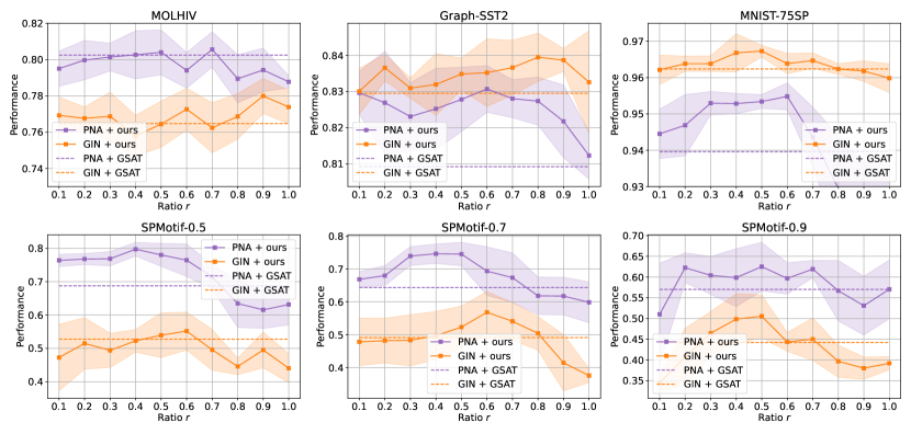
Figure 3: Hyperparameter sensitivity analysis of the sparsity $r$ in GSINA.

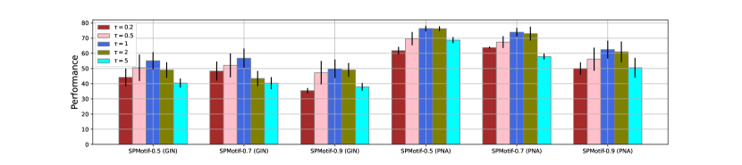
Figure 4: Hyperparameter sensitivity analysis of the temperature $\tau$ (for softness) in GSINA.

Performances Analysis. Tab. VII, VIII report the OOD generalization performances on CIGA benchmark. Our GSINA outperforms all the baselines of interpretable GNNs (ASAP, GIB, and DIR) by large margins. For the invariant learning baselines, our GSINA also achieves better performances. Compared with CIGA, GSINA achieves the best performances on SPMotif (except for -struct, $b=$ 0.33), Graph-SST5, Twitter, proteins and dd. On nci1, nci109, and DrugOOD datasets, GSINA produces results comparable to CIGA, indicating the difficulties of these OOD generalization tasks, meanwhile, the improvements of CIGA compared to ERM on DrugOOD datasets are also by little margin.

These improvements demonstrate the effectiveness of our softness and fully differentiability compared with CIGA (based on top-$k$). There are also large improvements observed on SPMotif datasets. Similar to Sec. IV-A, about 15% improvement than CIGA in classification accuracy on SPMotif (-mixed, $b=$ 0.9) in Tab. VII is observed.

IV-C Hyperparameter Studies

As shown in Fig. 3, for the 6 datasets used in the GSAT benchmark and reported in Tab. LABEL:tab:gsat, there are rough ‘increasing-decreasing’ patterns in the curve of predictive performance and subgraph ratio (i.e. sparsity) $r$, which reflects our GSINA is sensible to the hyperparameter $r$. The patterns of the curves in Fig. 3 show that a too-small or a too-large $r$ results in worse generalization. When $r$ is too small, it is more likely that the extracted subgraph $G_{S}$ is too sparse and lacks information; when $r$ is too large, it also results in a $G_{S}$ lack of information, as more redundant parts of the input graph $G$ would be selected, which results in a $G_{S}$ with little difference with $G$, and when $r=1.0$, GSINA degenerates to ERM with all edge attention set to 1.

As shown in Fig. 4, we analyze the hyperparameter sensitivity of the Sinkhorn temperature $\tau\in\{0.2,0.5,1,2,5\}$ on the SPMotif datasets (of GSAT benchmark, with both GIN and PNA backboned GSINA), which demonstrates $\tau=1$ is a reasonable and effective choice. When $\tau$ is too small, the model lacks softness and generates too ‘hard’ subgraphs; when $\tau$ is too large, the model is too soft and generates subgraphs that are too smooth and lack information. Both cases lead to reduced performances.

More Hyperparameter Settings. In our GSINA framework, we globally fix the Sinkhorn temperature $\tau$ (for softness) and Gumbel noise factor $\sigma$ (for randomness) to $1$, and the Sinkhorn iteration numbers to $10$.

TABLE IX: Dataset statistics of EERM benchmark used in experiments of Fig. 5, 6 and 7.

Dataset	Distribution Shift	#Nodes	#Edges	#Classes	Train/Val/Test Split	Metric	Adapted From
Cora		2,703	5,278	10	by graphs	Accuracy	[53]
Amazon-Photo	Artificial Transformation	7,650	119,081	10	by graphs	Accuracy	[32]
Twitch-explicit		1,912 - 9,498	31,299 - 153,138	2	by graphs	ROC-AUC	[31]
Facebook-100	Cross-Domain Transfers	769 - 41,536	16,656 - 1,590,655	2	by graphs	Accuracy	[37]
Elliptic		203,769	234,355	2	by time	F1 Score	[28]1
OGB-Arxiv	Temporal Evolution	169,343	1,166,243	40	by time	Accuracy	[16]

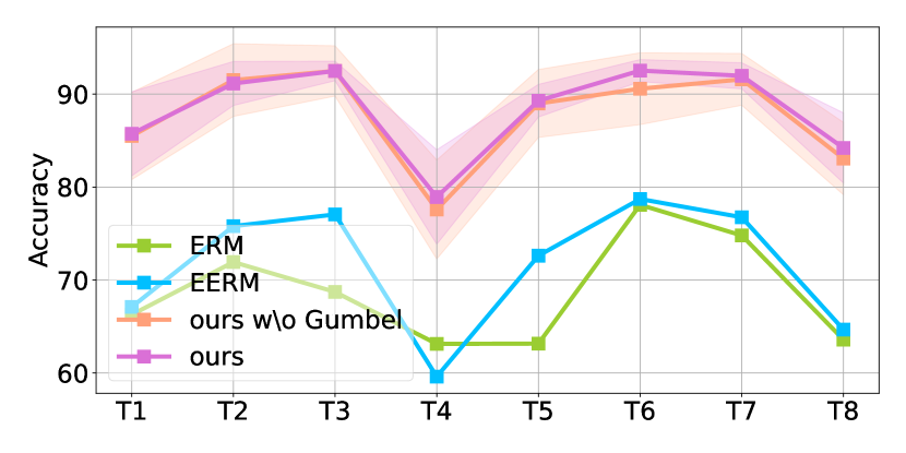
(a) Cora

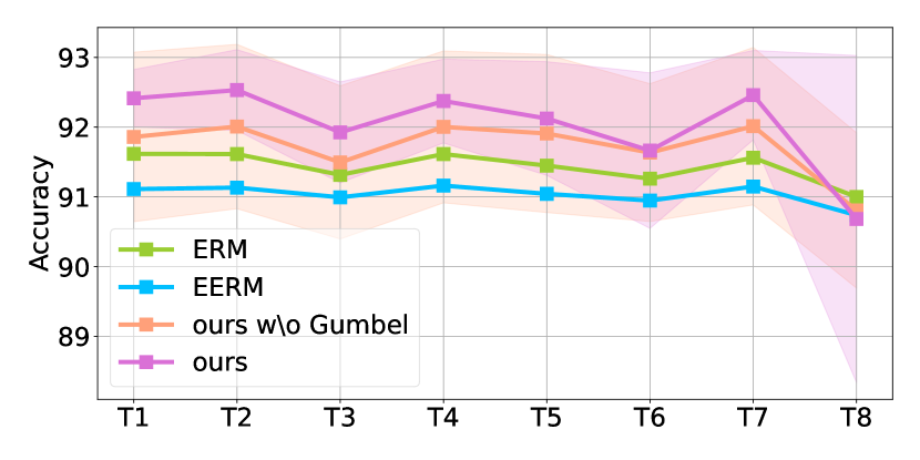
(b) Amazon-Photo

Figure 5: Node-level OOD generalization performances for ‘Artificial Transformation’.

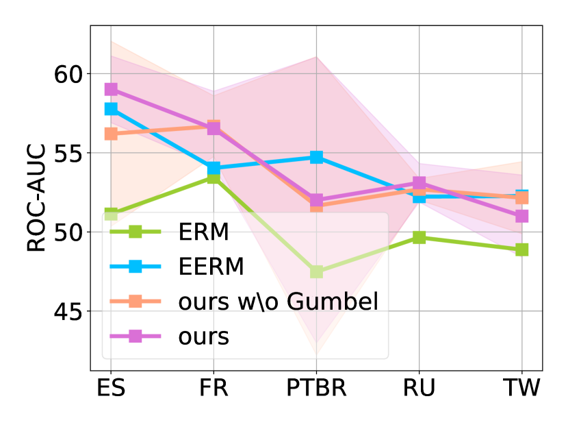
(a) Twitch-explicit

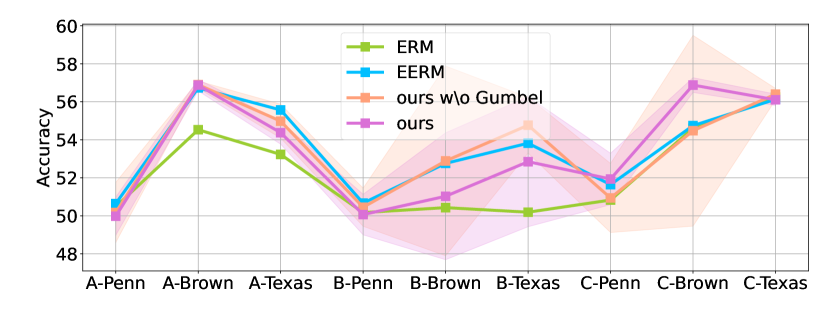
(b) Facebook-100

Figure 6: Node-level OOD generalization performances for ‘Cross-Domain Transfers’.

More Discussions. Our GSINA’s model selection procedure is simpler than CIGA (the ‘hard’ top-$k$ based GIL SOTA), with other settings fixed, what is required to tune to achieve SOTA performances in GSINA is just the sparsity $r$, while CIGA has additional loss balancing hyperparameters (2 losses corresponding to CIGAv1 and CIGAv2) to tune.

IV-D On Node-Level GIL Tasks

Datasets. We follow the datasets and protocols used in EERM [45], which involve 3 types of distribution shifts: 1) “Artificial Transformation”: synthetic spurious features are added to Cora and Amazon-Photo, and there are 8 testing graphs (T1 $\sim$ T8) for both datasets, 2) “Cross-Domain Transfers”: each graph in Twitch-explicit and Facebook-100 corresponds to distinct domains; for Twitch-explicit, DE is used for training, ENGB for validation and 5 graphs ES, FR, PTBR, RU, TW for testing; for Facebook-100, 3 different training sets are used, we denote them as A = (Johns Hopkins, Caltech, Amherst), B = (Bingham, Duke, Princeton), C = (WashU, Brandeis, Carnegie), the validation set is (Cornell, Yale), and the testing set is (Penn, Brown, Texas), 3) “Temporal Evolution”: train/val/test splits for Elliptic and OGB-Arxiv are made by time, Elliptic provides 9 test graphs (T1 $\sim$ T9), and OGB-Arxiv provides 3 time windows (14-16, 16-18, 18-20). The dataset details are shown in Tab. IX.

Metrics. We test the node classification accuracy (ACC) on Cora, Amazon-Photo, Facebook-100, OGB-Arxiv, ROC-AUC for Twitch-explicit, and F1-score for Elliptic.

Baselines. We compare our GSINA with ERM [38] and EERM [45], following the settings in EERM, we use GCN [20] as backbone subgraph extractors, predictors and spurious features generators (if applicable) for Cora, Amazon-Photo, Twitch-explicit and Facebook-100, SAGE [14] for Elliptic and OGB-Arxiv.

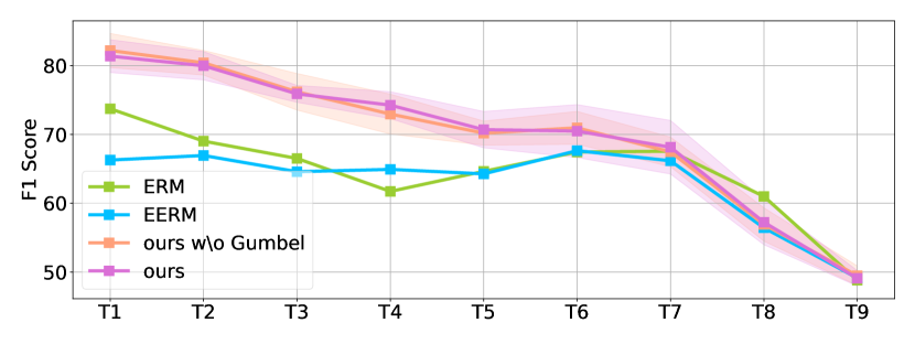
(a) Elliptic

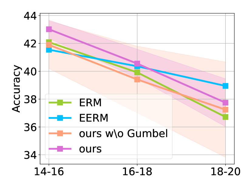
(b) OGB-Arxiv

Figure 7: Node-level OOD generalization performances for ‘Temporal Evolution’.

GNN Backbone Architectures. For GSINA with GCN and SAGE backbones for the experiments on EERM benchmark (reported in Fig. 5, 6, 7), our GNN backbone settings of GCN and SAGE are strictly in line with those in EERM settings, where we use ReLU as the activation, add self-loops and use batch normalization for graph convolution in each layer. We use 2 layers GCN with hidden size 32 for Cora, Amazon-Photo, Twitch-explicit, and Facebook-100; and 5 layers SAGE with hidden size 32 for Elliptic and OGB-Arxiv.

Optimization. For all datasets, we follow the AdamW optimizers used in EERM. To reproduce EERM results, we strictly follow the original settings of EERM. For the setting of our GSINA, we use the same settings with the experiments of ERM, where we use 0.01 learning rate for Cora, Amazon-Photo, and Twitch-explicit, 0.001 for Facebook-100, and 0.0002 for Elliptic.

Epoch. We follow the epochs used in EERM work and train to the end, which is 200 epochs for all datasets except for 500 epochs for OGB-Arxiv.

Hyperparameter Settings of $r$. According to the hyperparameter studies in Sec. IV-C, we regard $r=0.5$ as a reasonable choice and uniformly set it for all node classification experiments with our GSINA for simplicity.

Performances Analysis. Fig. 5, 6, 7 reports the generalization performance for the distribution shifts of ‘Artificial Transformation’, ‘Cross-Domain Transfers’, and ‘Temporal Evolution’, respectively. Under most testing scenarios, our GSINA outperforms ERM for node classification. We achieve better results than EERM on Cora, Amazon-Photo, Elliptic, and comparable results to EERM on Twitch-explicit, Facebook-100, and OGB-Arxiv. Especially, our GSINA achieves an improvement of about 20% for classification accuracy on Cora.

IV-E Ablation Studies

We provide our ablation studies on both graph and node classification tasks. Tab. X reports detailed experiment results on SPMotif datasets in the GSAT benchmark, the ablation versions of our GSINA are without (w/o) the Gumbel noise, Node Attention, or both (denoted as G & N), with the same $r$ as the full GSINA (note that it is not necessary the optimal $r$ for these ablation versions). As the Node Attention is not required for node classification tasks, the ablation studies in Fig. 5, 6, 7 only provide the version without the Gumbel noise.

From the ablation studies, we observe performance degradations for graph and node level tasks when learning GSINA without Gumbel noise, Node Attention, or both, demonstrating the effectiveness of the proposed components of GSINA. Moreover, in the node classification tasks, the ablation versions provide higher variances on Cora, Amazon-Photo, and OGB-Arxiv, which demonstrate the Gumbel trick could stabilize the learning of GSINA.

TABLE X: Ablation studies on SPMotif datasets.

	Spurious-motif
	$b=0.5$	$b=0.7$	$b=0.9$
GIN+ours	$\mathbf{55.16}{\scriptstyle\pm 5.69}$	$\mathbf{56.83}{\scriptstyle\pm 6.32}$	${49.86}{\scriptstyle\pm 6.10}$
w/o Gumbel	$48.27{\scriptstyle\pm 4.80}$	$45.25{\scriptstyle\pm 7.15}$	$\mathbf{50.28}{\scriptstyle\pm 2.83}$
w/o NodeAttn	$47.34{\scriptstyle\pm 7.99}$	$54.63{\scriptstyle\pm 6.99}$	$48.41{\scriptstyle\pm 1.16}$
w/o G&N	$46.28{\scriptstyle\pm 5.67}$	$45.40{\scriptstyle\pm 3.22}$	$44.44{\scriptstyle\pm 6.56}$
GIN+GSAT	$52.74{\scriptstyle\pm 4.08}$	$49.12{\scriptstyle\pm 3.29}$	$44.22{\scriptstyle\pm 5.57}$
PNA+ours	$\mathbf{76.39}{\scriptstyle\pm 1.85}$	$\mathbf{73.96}{\scriptstyle\pm 2.87}$	$\mathbf{62.51}{\scriptstyle\pm 5.86}$
w/o Gumbel	$69.95{\scriptstyle\pm 2.76}$	$69.67{\scriptstyle\pm 3.44}$	$62.14{\scriptstyle\pm 4.64}$
w/o NodeAttn	$71.60{\scriptstyle\pm 1.89}$	$58.70{\scriptstyle\pm 3.82}$	$58.20{\scriptstyle\pm 2.70}$
w/o G&N	$71.75{\scriptstyle\pm 2.42}$	$67.50{\scriptstyle\pm 4.51}$	$61.34{\scriptstyle\pm 1.72}$
PNA+GSAT	$68.74{\scriptstyle\pm 2.24}$	$64.38{\scriptstyle\pm 3.20}$	$57.01{\scriptstyle\pm 2.95}$

IV-F Runtime and Complexity Analysis

Our GSINA has two different settings for subgraph extraction in a batch (we always selected the better one for experiments). The first (denoted as micro) setting is to compute soft top-$r$ for each graph in the batch, which is slower, we use it on Spmotif, TU-PROT, TU-DD, Graph-SST2, MNIST-75sp, OGBG-Molbbbp, OGBG-Molclintox, OGBG-Moltox21, OGBG-Molsider. The second (denoted as macro) setting is to compute soft top-$r$ just once for the entire batch (which can be considered as a large graph composed of several smaller graphs), which is faster, we use it on Graph-SST5, Twitter, Drug-Assay, Drug-Sca, Drug-Size, TU-NCI1, TU-NCI109, OGBG-Molhiv, OGBG-Molbace. The macro setting computes the top-$r$ for the whole graph and relaxes the constraint of top-$r$ on each individual graph, which is useful when the distribution shifts are complicated, and in that case, it is difficult to find a uniform reasonable $r$ for each graph. Therefore, the macro vs micro model selection in GSINA is highly dependent on the characteristics of the dataset, and we select the one with better performance for each dataset. On the other hand, CIGA uses hard top-$k$ selection for subgraph extraction for each graph (similar to the micro setting) in the batch. And we have implemented GSAT (note that it is without hyperparameter tuning) on the CIGA benchmark for training time comparison, GSAT is similar to the macro setting to an extent, GSAT models the probability $p$ of each edge belonging to the invariant part, while does not consider how many graphs are in the batch.

TABLE XI: Training time comparison on CIGA benchmark, we record the training time in terms of s/epoch.

	Spmotif	Graph-SST5	Twitter	Drug-Assay	Drug-Sca	Drug-Size	TU-NCI1	TU-NCI109	TU-PROT	TU-DD
ERM	$5.80{\scriptstyle\pm 0.22}$	$3.99{\scriptstyle\pm 0.10}$	$2.12{\scriptstyle\pm 0.29}$	$9.77{\scriptstyle\pm 2.12}$	$6.70{\scriptstyle\pm 0.66}$	$10.81{\scriptstyle\pm 1.10}$	$1.26{\scriptstyle\pm 0.07}$	$1.22{\scriptstyle\pm 0.08}$	$0.40{\scriptstyle\pm 0.08}$	$0.37{\scriptstyle\pm 0.09}$
GSAT	$11.08{\scriptstyle\pm 0.29}$	$7.74{\scriptstyle\pm 0.08}$	$4.13{\scriptstyle\pm 0.14}$	$17.03{\scriptstyle\pm 0.66}$	$10.85{\scriptstyle\pm 0.60}$	$17.95{\scriptstyle\pm 1.07}$	$2.45{\scriptstyle\pm 0.10}$	$2.39{\scriptstyle\pm 0.08}$	$0.71{\scriptstyle\pm 0.08}$	$0.72{\scriptstyle\pm 0.09}$
GSINA-macro	$14.80{\scriptstyle\pm 0.32}$	$9.50{\scriptstyle\pm 0.23}$	$5.21{\scriptstyle\pm 0.13}$	$19.83{\scriptstyle\pm 1.24}$	$12.68{\scriptstyle\pm 0.67}$	$23.15{\scriptstyle\pm 1.54}$	$3.14{\scriptstyle\pm 0.12}$	$3.00{\scriptstyle\pm 0.09}$	$0.89{\scriptstyle\pm 0.07}$	$1.04{\scriptstyle\pm 0.06}$
CIGA	$21.66{\scriptstyle\pm 0.91}$	$14.34{\scriptstyle\pm 0.25}$	$7.96{\scriptstyle\pm 0.21}$	$54.83{\scriptstyle\pm 1.22}$	$33.74{\scriptstyle\pm 0.62}$	$58.45{\scriptstyle\pm 0.92}$	$5.01{\scriptstyle\pm 0.13}$	$4.48{\scriptstyle\pm 0.05}$	$1.19{\scriptstyle\pm 0.08}$	$1.36{\scriptstyle\pm 0.11}$
GSINA-micro	$34.58{\scriptstyle\pm 0.63}$	$24.52{\scriptstyle\pm 0.37}$	$13.04{\scriptstyle\pm 0.21}$	$97.43{\scriptstyle\pm 3.12}$	$59.47{\scriptstyle\pm 0.69}$	$101.28{\scriptstyle\pm 0.75}$	$7.43{\scriptstyle\pm 0.11}$	$7.37{\scriptstyle\pm 0.13}$	$1.93{\scriptstyle\pm 0.09}$	$2.14{\scriptstyle\pm 0.11}$

We conducted experiments on the training time of the models on all datasets of the CIGA benchmark. In Tab. XI, we report experimental results of training time comparison on CIGA benchmark, ERM is always the fastest, and our second setting (GSINA-macro) is often much faster than CIGA and a bit slower than GSAT due to iterative computations (Eq. 6); while the first setting (GSINA-micro), also due to iterative computations (Eq. 6) in subgraph extraction, is slower than CIGA’s hard top-k selection. However, since we can set the number of iterations to a relatively small value (we uniformly used 10), GSINA does not introduce a significant computing overhead and is always within 2 $\times$ CIGA’s complexity.

IV-G Further Discussions

TABLE XII: Interpretation Performance (AUC).

	Spurious-motif
	$b=0.5$	$b=0.7$	$b=0.9$
GNNExplainer	$62.62{\scriptstyle\pm 1.35}$	$62.25{\scriptstyle\pm 3.61}$	$58.86{\scriptstyle\pm 1.93}$
PGExplainer	$69.54{\scriptstyle\pm 5.64}$	$72.33{\scriptstyle\pm 9.18}$	${72.34}{\scriptstyle\pm 2.91}$
GraphMask	$72.06{\scriptstyle\pm 5.58}$	$73.06{\scriptstyle\pm 4.91}$	$66.68{\scriptstyle\pm 6.96}$
GIB [54]	$57.29{\scriptstyle\pm 14.35}$	$62.89{\scriptstyle\pm 15.59}$	$47.29{\scriptstyle\pm 13.39}$
DIR [46]	${78.15}{\scriptstyle\pm 1.32}$	${77.68}{\scriptstyle\pm 1.22}$	$49.08{\scriptstyle\pm 3.66}$
GIN+GSAT	$\underline{78.45}{\scriptstyle\pm 3.12}$	$74.07{\scriptstyle\pm 5.28}$	$71.97{\scriptstyle\pm 4.41}$
GIN+ours	$65.13{\scriptstyle\pm 10.00}$	$60.78{\scriptstyle\pm 8.09}$	$55.86{\scriptstyle\pm 3.56}$
PNA+GSAT	$\mathbf{83.34}{\scriptstyle\pm 2.17}$	$\mathbf{86.94}{\scriptstyle\pm 4.05}$	$\mathbf{88.66}{\scriptstyle\pm 2.44}$
PNA+ours	$75.66{\scriptstyle\pm 1.56}$	$\underline{80.47}{\scriptstyle\pm 1.06}$	$\underline{80.10}{\scriptstyle\pm 2.04}$

TABLE XIII: Interpretation precision@5 of with the GNN backbone ‘SPMotifNet’ in DIR [46].

	Spurious-motif
	$b=0.5$	$b=0.7$	$b=0.9$
GNNExplainer	$0.203\scriptstyle{\pm 0.019}$	$0.167\scriptstyle{\pm 0.039}$	$0.066\scriptstyle{\pm 0.007}$
DIR [46]	$0.255\scriptstyle{\pm 0.016}$	$0.247\scriptstyle{\pm 0.012}$	$0.192\scriptstyle{\pm 0.044}$
GSAT [26]	$\mathbf{0.519}\scriptstyle{\pm 0.022}$	$\mathbf{0.503}\scriptstyle{\pm 0.034}$	$\underline{0.416}\scriptstyle{\pm 0.081}$
ours	$\underline{0.419}\scriptstyle{\pm 0.030}$	$\underline{0.401}\scriptstyle{\pm 0.046}$	$\mathbf{0.429}\scriptstyle{\pm 0.040}$

Subgraph Interpretability Discussions. In addition to the generalizability detailedly discussed above, for the completeness of this paper, here we discuss the interpretability of our GSINA with regard to the accuracy of the invariant subgraph extraction, although our interpretability is inferior. The interpretability is evaluated based on SPMotif datasets, which have labeled ground truths of explanation subgraphs (a.k.a invariant subgraphs $G_{S}$). The interpretability evaluation metrics are following previous studies DIR [46] and GSAT [26] for the performance of explanation subgraph recognition, which is a problem of binary classification for each edge. Following DIR and GSAT, we perform edge binary classifications, for metrics, we evaluate ROC-AUC (with GIN and PNA backbones, following the setting of GSAT) and precision@5 (with the GNN backbone ‘SPMotifNet’ used in DIR [46]).

As shown in Tab. LABEL:tab:xauc, LABEL:tab:prec5, our GSINA (PNA and SPMotifNet backbones) mostly outperform interpretable GNNs DIR and GIB as well as other post-hoc [26] GNN explainers, showing our inherent interpretability to extract invariant subgraphs. However, our GSINA is inferior to GSAT in interpretability, we tend to believe that it is due to the innate characteristics of top-$k$ based methods: intuitively, for a ‘hard’ top-$k$, the output value is binary (0 / 1), meaning an item belongs to top-$k$ or not, ‘hard’ top-$k$ does not consider the relative ranking of items at all, while the prevalent metrics for binary classification (e.g. AUC, precision@5) always do. Hence, it is not natural to evaluate the subgraph recognition performance of top-$k$ based methods. However, GSAT does not restrict edge predictions to (approximated) binary like top-$k$ methods, so that it achieves more flexible edge attention weights and better performance in interpretability. Due to the utilization of soft top-$r$ operation in GSINA, it places more mathematical constraints on the graph attention value distribution compared to GSAT. The choice of $r$ in GSINA significantly impacts the attention distribution, whereas GSAT is not subject to this issue. To sum up, the design of GSAT, as mentioned above, is a tradeoff. It excels in interpretability, but it falls short in effectively filtering out variant parts (as described in Sec. I, Fig. 1). This leads to GSAT having a less optimal ability to make predictions using subgraphs compared to GSINA.

Subgraph Property Discussions. In this paper, we have taken three meaningful properties: sparsity, softness, and differentiability, into consideration to improve the invariant subgraph extraction for GIL methods. However, it is definitely not the final solution of the GIL subgraph extraction. There might be other interesting considerations of how the extracted invariant subgraph should be, such as subgraph connectivity or completeness, as it might be expected that the invariant regions should represent coherent structures and patterns rather than disjoint disconnected components. For such considerations, we would like to provide elementary solutions and discuss the difficulties of the problems.

Regarding the issue of subgraph connectivity, we believe it depends on the characteristics of the data. The crucial subgraphs might be either connected or not, for example, a molecule may have multiple disconnected functional groups playing a key role. Connectivity was not explicitly considered in our GSINA design, if desired, a penalty loss (like the connectivity loss in GIB [54]) could be added to our learning objective in Sec. III-A to enhance connectivity. However, the subgraph is latent and inferred by the GNN from data, the understanding of data by the model does not necessarily have to be consistent with that of humans. On the other hand, what humans consider a ‘complete subgraph’ may still have redundant parts in the model’s learning process. It is difficult for us to determine definitively which nodes or edges should be included in a ‘complete invariant subgraph’. Moreover, since many datasets may lack ground-truth information about the invariant subgraph, it is also challenging to define a metric or penalty loss for completeness. Currently, even without a guarantee of subgraph connectivity or completeness, GSINA could still improve GIL performances based on its extracted subgraphs.

V Conclusion

In this paper, we have proposed Graph Sinkhorn Attention (GSINA), a general invariance optimization framework for Graph Invariant Learning (GIL) to improve the generalization for both graph and node level tasks by extracting the sparse, soft, and differentiable invariant subgraphs in the manner of graph attention. Extensive experiments have shown the superiority of GSINA against the state-of-the-arts on both graph and node level GIL tasks.

References

- [1] Kartik Ahuja, Ethan Caballero, Dinghuai Zhang, Jean-Christophe Gagnon-Audet, Yoshua Bengio, Ioannis Mitliagkas, and Irina Rish. Invariance principle meets information bottleneck for out-of-distribution generalization. Advances in Neural Information Processing Systems, 34:3438–3450, 2021.
- [2] Martin Arjovsky, Léon Bottou, Ishaan Gulrajani, and David Lopez-Paz. Invariant risk minimization. arXiv preprint arXiv:1907.02893, 2019.
- [3] Giorgio Ausiello, Pierluigi Crescenzi, Giorgio Gambosi, Viggo Kann, Alberto Marchetti-Spaccamela, and Marco Protasi. Complexity and approximation: Combinatorial optimization problems and their approximability properties. Springer Science & Business Media, 2012.
- [4] Beatrice Bevilacqua, Yangze Zhou, and Bruno Ribeiro. Size-invariant graph representations for graph classification extrapolations. In International Conference on Machine Learning, pages 837–851. PMLR, 2021.
- [5] Davide Buffelli, Pietro Liò, and Fabio Vandin. Sizeshiftreg: a regularization method for improving size-generalization in graph neural networks. arXiv preprint arXiv:2207.07888, 2022.
- [6] T-J Chang, Nigel Meade, John E Beasley, and Yazid M Sharaiha. Heuristics for cardinality constrained portfolio optimisation. Computers & Operations Research, 27(13):1271–1302, 2000.
- [7] Wei Chen, Xiaoming Sun, Jialin Zhang, and Zhijie Zhang. Network inference and influence maximization from samples. In International Conference on Machine Learning, pages 1707–1716. PMLR, 2021.
- [8] Yongqiang Chen, Yonggang Zhang, Yatao Bian, Han Yang, MA Kaili, Binghui Xie, Tongliang Liu, Bo Han, and James Cheng. Learning causally invariant representations for out-of-distribution generalization on graphs. Advances in Neural Information Processing Systems, 35:22131–22148, 2022.
- [9] Yongqiang Chen, Yonggang Zhang, Han Yang, Kaili Ma, Binghui Xie, Tongliang Liu, Bo Han, and James Cheng. Invariance principle meets out-of-distribution generalization on graphs. arXiv preprint arXiv:2202.05441, 2022.
- [10] Gabriele Corso, Luca Cavalleri, Dominique Beaini, Pietro Liò, and Petar Veličković. Principal neighbourhood aggregation for graph nets. In Advances in Neural Information Processing Systems, pages 13260–13271, 2020.
- [11] Elliot Creager, Jörn-Henrik Jacobsen, and RichardS. Zemel. Environment inference for invariant learning, Oct 2020.
- [12] Marco Cuturi. Sinkhorn distances: Lightspeed computation of optimal transport. In C.J. Burges, L. Bottou, M. Welling, Z. Ghahramani, and K.Q. Weinberger, editors, Advances in Neural Information Processing Systems, volume 26. Curran Associates, Inc., 2013.
- [13] Li Dong, Furu Wei, Chuanqi Tan, Duyu Tang, Ming Zhou, and Ke Xu. Adaptive recursive neural network for target-dependent twitter sentiment classification. In Proceedings of the 52nd Annual Meeting of the Association for Computational Linguistics (Volume 2: Short Papers), Jun 2015.
- [14] Will Hamilton, Zhitao Ying, and Jure Leskovec. Inductive representation learning on large graphs. Advances in neural information processing systems, 30, 2017.
- [15] Weihua Hu, Matthias Fey, Marinka Zitnik, Yuxiao Dong, Hongyu Ren, Bowen Liu, Michele Catasta, and Jure Leskovec. Open graph benchmark: Datasets for machine learning on graphs. In Advances in Neural Information Processing Systems, pages 22118–22133, 2020.
- [16] Weihua Hu, Matthias Fey, Marinka Zitnik, Yuxiao Dong, Hongyu Ren, Bowen Liu, Michele Catasta, and Jure Leskovec. Open graph benchmark: Datasets for machine learning on graphs. In Advances in Neural Information Processing Systems (NeurIPS), 2020.
- [17] Eric Jang, Shixiang Gu, and Ben Poole. Categorical reparameterization with gumbel-softmax. In International Conference on Learning Representations, 2017.
- [18] Yuanfeng Ji, Lu Zhang, Jiaxiang Wu, Bingzhe Wu, Long-Kai Huang, Tingyang Xu, Yu Rong, Lanqing Li, Jie Ren, Ding Xue, et al. Drugood: Out-of-distribution (ood) dataset curator and benchmark for ai-aided drug discovery–a focus on affinity prediction problems with noise annotations. arXiv preprint arXiv:2201.09637, 2022.
- [19] Nikolaos Karalias and Andreas Loukas. Erdos goes neural: an unsupervised learning framework for combinatorial optimization on graphs. Advances in Neural Information Processing Systems, 33:6659–6672, 2020.
- [20] Thomas N Kipf and Max Welling. Semi-supervised classification with graph convolutional networks. arXiv preprint arXiv:1609.02907, 2016.
- [21] Boris Knyazev, Graham W Taylor, and Mohamed Amer. Understanding attention and generalization in graph neural networks. In Advances in Neural Information Processing Systems, pages 4204–4214, 2019.
- [22] David Krueger, Ethan Caballero, Joern-Henrik Jacobsen, Amy Zhang, Jonathan Binas, Dinghuai Zhang, Remi Le Priol, and Aaron Courville. Out-of-distribution generalization via risk extrapolation (REx). In International Conference on Machine Learning, pages 5815–5826. PMLR, 2021.
- [23] Haoyang Li, Xin Wang, Ziwei Zhang, and Wenwu Zhu. Out-of-distribution generalization on graphs: A survey. arXiv preprint arXiv:2202.07987, 2022.
- [24] Haoyang Li, Ziwei Zhang, Xin Wang, and Wenwu Zhu. Learning invariant graph representations for out-of-distribution generalization. In Advances in Neural Information Processing Systems, 2022.
- [25] J. Ma, P. Cui, K. Kuang, X. Wang, and W. Zhu. Disentangled graph convolutional networks. In International Conference on Machine Learning, 2019.
- [26] Siqi Miao, Mia Liu, and Pan Li. Interpretable and generalizable graph learning via stochastic attention mechanism. In International Conference on Machine Learning, pages 15524–15543. PMLR, 2022.
- [27] Christopher Morris, Nils M Kriege, Franka Bause, Kristian Kersting, Petra Mutzel, and Marion Neumann. Tudataset: A collection of benchmark datasets for learning with graphs. arXiv preprint arXiv:2007.08663, 2020.
- [28] Aldo Pareja, Giacomo Domeniconi, Jie Chen, Tengfei Ma, Toyotaro Suzumura, Hiroki Kanezashi, Tim Kaler, Tao B. Schardl, and Charles E. Leiserson. Evolvegcn: Evolving graph convolutional networks for dynamic graphs. In AAAI Conference on Artificial Intelligence (AAAI), pages 5363–5370, 2020.
- [29] Gabriel Peyré, Marco Cuturi, et al. Computational optimal transport: With applications to data science. Foundations and Trends® in Machine Learning, 11(5-6):355–607, 2019.
- [30] Ekagra Ranjan, Soumya Sanyal, and Partha Pratim Talukdar. ASAP: Adaptive structure aware pooling for learning hierarchical graph representations. arXiv preprint arXiv:1911.07979, 2019.
- [31] Benedek Rozemberczki, Carl Allen, and Rik Sarkar. Multi-scale attributed node embedding. Journal of Complex Networks, 9(2), 2021.
- [32] Oleksandr Shchur, Maximilian Mumme, Aleksandar Bojchevski, and Stephan Günnemann. Pitfalls of graph neural network evaluation. CoRR, abs/1811.05868, 2018.
- [33] Richard Sinkhorn. A relationship between arbitrary positive matrices and doubly stochastic matrices. Annals of Mathematical Statistics, 35:876–879, 1964.
- [34] Richard Socher, Alex Perelygin, Jean Wu, Jason Chuang, Christopher D Manning, Andrew Y Ng, and Christopher Potts. Recursive deep models for semantic compositionality over a sentiment treebank. In Proceedings of the conference on empirical methods in natural language processing, pages 1631–1642, 2013.
- [35] Yongduo Sui, Xiang Wang, Jiancan Wu, Min Lin, Xiangnan He, and Tat-Seng Chua. Causal attention for interpretable and generalizable graph classification. In Proceedings of the 28th ACM SIGKDD Conference on Knowledge Discovery and Data Mining, pages 1696–1705, 2022.
- [36] Naftali Tishby and Noga Zaslavsky. Deep learning and the information bottleneck principle. In 2015 ieee information theory workshop (itw), pages 1–5. IEEE, 2015.
- [37] Amanda L. Traud, Peter J. Mucha, and Mason A. Porter. Social structure of facebook networks. CoRR, abs/1102.2166, 2011.
- [38] Vladimir Vapnik. Principles of risk minimization for learning theory, Dec 1991.
- [39] P. Velikovi, G. Cucurull, A. Casanova, A. Romero, P Liò, and Y. Bengio. Graph attention networks. In International Conference on Learning Representations, 2018.
- [40] Petar Veličković, Guillem Cucurull, Arantxa Casanova, Adriana Romero, Pietro Liò, and Yoshua Bengio. Graph attention networks, 2018.
- [41] Cédric Villani et al. Optimal transport: old and new, volume 338. Springer, 2009.
- [42] Daixin Wang, Jianbin Lin, Peng Cui, Quanhui Jia, Zhen Wang, Yanming Fang, Quan Yu, Jun Zhou, Shuang Yang, and Yuan Qi. A semi-supervised graph attentive network for financial fraud detection. In 2019 IEEE International Conference on Data Mining (ICDM), pages 598–607. IEEE, 2019.
- [43] Runzhong Wang, Li Shen, Yiting Chen, Xiaokang Yang, Dacheng Tao, and Junchi Yan. Towards one-shot neural combinatorial solvers: Theoretical and empirical notes on the cardinality-constrained case. In The Eleventh International Conference on Learning Representations, 2023.
- [44] Joanna Wencel-Delord and Frank Glorius. C–h bond activation enables the rapid construction and late-stage diversification of functional molecules. Nature chemistry, 5(5):369–375, 2013.
- [45] Qitian Wu, Hengrui Zhang, Junchi Yan, and David Wipf. Handling distribution shifts on graphs: An invariance perspective. arXiv preprint arXiv:2202.02466, 2022.
- [46] Yingxin Wu, Xiang Wang, An Zhang, Xiangnan He, and Tat-Seng Chua. Discovering invariant rationales for graph neural networks. In International Conference on Learning Representations, 2022.
- [47] Zhenqin Wu, Bharath Ramsundar, Evan N Feinberg, Joseph Gomes, Caleb Geniesse, Aneesh S Pappu, Karl Leswing, and Vijay Pande. Moleculenet: a benchmark for molecular machine learning. Chemical science, 9(2):513–530, 2018.
- [48] Yujia Xie, Hanjun Dai, Minshuo Chen, Bo Dai, Tuo Zhao, Hongyuan Zha, Wei Wei, and Tomas Pfister. Differentiable top-k operator with optimal transport, 2020.
- [49] Yujia Xie, Hanjun Dai, Minshuo Chen, Bo Dai, Tuo Zhao, Hongyuan Zha, Wei Wei, and Tomas Pfister. Differentiable top-k with optimal transport. In Neural Information Processing Systems, 2020.
- [50] Keyulu Xu, Weihua Hu, Jure Leskovec, and Stefanie Jegelka. How powerful are graph neural networks? arXiv preprint arXiv:1810.00826, 2018.
- [51] Nianzu Yang, Kaipeng Zeng, Qitian Wu, Xiaosong Jia, and Junchi Yan. Learning substructure invariance for out-of-distribution molecular representations. In Advances in Neural Information Processing Systems, 2022.
- [52] Shuo Yang, Zhiqiang Zhang, Jun Zhou, Yang Wang, Wang Sun, Xingyu Zhong, Yanming Fang, Quan Yu, and Yuan Qi. Financial risk analysis for smes with graph-based supply chain mining. In Proceedings of the Twenty-Ninth International Conference on International Joint Conferences on Artificial Intelligence, pages 4661–4667, 2021.
- [53] Zhilin Yang, William W. Cohen, and Ruslan Salakhutdinov. Revisiting semi-supervised learning with graph embeddings. In International Conference on Machine Learning (ICML), pages 40–48, 2016.
- [54] Junchi Yu, Tingyang Xu, Yu Rong, Yatao Bian, Junzhou Huang, and Ran He. Graph information bottleneck for subgraph recognition. arXiv preprint arXiv:2010.05563, 2020.
- [55] Hao Yuan, Haiyang Yu, Shurui Gui, and Shuiwang Ji. Explainability in graph neural networks: A taxonomic survey. arXiv preprint arXiv:2012.15445, 2020.
-
[56]
Michael Zhang, NimitS. Sohoni, HongyangR. Zhang, Chelsea Finn, and Christopher R
’e. Correct-n-contrast: A contrastive approach for improving robustness to spurious correlations. - [57] Yanfu Zhang, Shangqian Gao, Jian Pei, and Heng Huang. Improving social network embedding via new second-order continuous graph neural networks. In Proceedings of the 28th ACM SIGKDD Conference on Knowledge Discovery and Data Mining, pages 2515–2523, 2022.
- [58] Qi Zhu, Natalia Ponomareva, Jiawei Han, and Bryan Perozzi. Shift-robust GNNs: Overcoming the limitations of localized graph training data. Advances in Neural Information Processing Systems, 34, 2021.