“To renormalize or not to renormalize ?” in the proton-deuteron scattering calculations

Abstract

We discuss two approaches which, by applying the screening method, permit one to include the long range proton-proton (pp) Coulomb force in proton-deuteron (pd) momentum-space scattering calculations. In the first one, based on Alt-Grassberger-Sandhas (AGS) equation, presented in Phys. Rev. C71, 054005 (2005) and 73, 057001 (2006), one needs to renormalize elastic scattering amplitude before calculating observables. In the second treatment, proposed by us in Eur. Phys. Journal A 41, 369 (2009), 41, 385 (2009), and arXiv:2310.03433 [nucl.th], this renormalization is avoided. For the proton induced deuteron breakup reaction both approaches require renormalization of the corresponding transition amplitudes. We derive the basic equations underlying both methods under the assumption that all contributing partial wave states are included and explain why in our approach renormalization of the elastic scattering amplitude is superfluous. We show that in order to take into account in the screening limit all partial waves it is required that four additional terms, based on the 3-dimensional and partial-wave projected pp Coulomb t-matrices, identical for both approaches, must appear in transition amplitudes. We investigate importance of these terms for elastic pd scattering below the breakup threshold.

The Hamlet-like question in the title arose when two preprints  [1] and  [2], both dealing with the problem how to include the long range proton-proton (pp) Coulomb force in momentum space pd scattering calculations through a screened Coulomb interaction, were posted. The arguments presented in  [2] show that in the well established approach of Refs. [3, 4] the interplay of the pp Coulomb potential and the deuteron bound state pole in the neutron-proton t-matrix makes renormalization of the elastic scattering transition amplitude necessary prior to calculating observables. Contrary to that, in our approach presented in  [1, 5, 6], one avoids such renormalization. In the following we explain similarities and differences of both treatments and provide justification why the renormalization in our method for elastic scattering is unnecessary. We also discuss a very important problem, indispensable in any treatment of the long-range Coulomb force: how to take into account, in addition to partial waves utilised when solving corresponding three-nucleon (3N) scattering equations, all higher partial wave states.

Let us start with the well established approach of Refs. [3, 4] based on the AGS equation for the pd transition operator $U$  [7, 8]:

$$U\left|{\Phi}\right\rangle=PG_{0}^{-1}\left|{\Phi}\right\rangle+PtG_{0}U\left|{\Phi}\right\rangle~{},$$ (1)

where $P$ is defined in terms of transposition operators, $P=P_{12}P_{23}+P_{13}P_{23}$, $G_{0}$ is the free 3N propagator and $|\Phi>$ is the initial state composed of a deuteron and a momentum eigenstate of the proton. The t-matrix $t$ is a solution of the 2-body Lippmann-Schwinger (LS) equation, with the interaction which contains in case of the pp system in addition to the nuclear part also the Coulomb pp force (assumed to be screened and parametrized by some parameter $R$). If the state $U|\Phi>$ is known, the elastic pd scattering amplitude $<\Phi~{}^{\prime}|U|\Phi>$, with $|\Phi~{}^{\prime}>$ being the final pd state, can be obtained by quadratures in the standard manner.

In our approach we use the breakup operator T defined as:

$$T=tG_{0}U~{}.$$ (2)

It fulfills the 3N Faddeev equation which, when nucleons interact with pairwise forces only, is given by  [9, 8]:

$$T|\Phi>=tP|\Phi>+tPG_{0}T|\Phi>~{}.$$ (3)

The above form of the Faddeev equation ensures that the T operator reflects directly the properties of the t-matrix. Here the elastic scattering amplitude is calculated from solutions of (3) by  [8, 9]:

$$\left\langle{\Phi^{\prime}}\right|U\left|{\Phi}\right\rangle = \left\langle{\Phi^{\prime}}\right|PG_{0}^{-1}\left|{\Phi}\right\rangle+\left\langle{\Phi^{\prime}}\right|PT\left|{\Phi}\right\rangle~{},$$ (4)

and the transition amplitude for breakup $<\Phi_{0}|U_{0}|\Phi>$ is expressed in terms of $T\left|{\Phi}\right\rangle$ by [8, 9]

$$\left\langle{\Phi_{0}}\right|U_{0}\left|{\Phi}\right\rangle = \left\langle{\Phi_{0}}\right|(1+P)T\left|{\Phi}\right\rangle~{},$$ (5)

where $|\Phi_{0}>=|\vec{p}\,\vec{q}\,m_{1}m_{2}m_{3}\nu_{1}\nu_{2}\nu_{3}>$ is the state of three free outgoing nucleons. In the approach based on the AGS equation the transition amplitude for breakup is given also by Eq. (5) but with T replaced by U.

The AGS, (1), as well as the Faddeev, (3), equations are solved in the momentum-space partial-wave basis $|pq\bar{\alpha}>$:

$$|pq\bar{\alpha}>\equiv|pq(ls)j(\lambda\frac{1}{2})I(jI)J(t\frac{1}{2})T>~{},$$ (6)

where one can differentiate between the partial wave states $|pq\alpha>$ with total 2N angular momentum $j$ below some value $j_{max}$: $j\leq j_{max}$, in which the nuclear, $V_{N}$, as well as the pp screened Coulomb interaction, $V_{c}^{R}$ (in isospin $t=1$ states only), act, and the states $|pq\beta>$ with $j>j_{max}$, for which only the screened Coulomb force $V_{c}^{R}$ is present in the pp subsystem. Incorporation of the $|pq\beta>$ states is indispensable due to the long range nature of the pp Coulomb force and the necessity to perform finally the screening limit $R\to\infty$. In the following we derive for both approaches the equations in a subspace restricted to $|pq\alpha>$ states only, which, however, incorporate all contributions from the complementary subspace of $|pq\beta>$ states. The states $|pq\alpha>$ and $|pq\beta>$ form together a complete system of states (in the following we use shorthand notation $\sum\limits_{\alpha}{\int{p^{2}dpq^{2}dq\left|{pq\alpha}\right\rangle\left\langle{pq\alpha}\right|}}\equiv{\left|{\alpha}\right\rangle\left\langle{\alpha}\right|}$):

$$\int{p^{2}dpq^{2}dq}(\sum\limits_{\alpha}{\left|{pq\alpha}\right\rangle}\left\langle{pq\alpha}\right|+\sum\limits_{\beta}{\left|{pq\beta}\right\rangle}\left\langle{pq\beta}\right|)={\left|{\alpha}\right\rangle\left\langle{\alpha}\right|}+{\left|{\beta}\right\rangle\left\langle{\beta}\right|}={\rm I}\\ ~{}$$ (7)

where I is the identity operator.

Let us start with our approach. Projecting Eq. (3) for $T|\Phi>$ on the $|pq\alpha>$ and $|pq\beta>$ states one gets the following system of coupled integral equations  [1]:

$$\left\langle{pq\alpha}\right|T\left|{\Phi}\right\rangle = \left\langle{pq\alpha}\right|t_{N+c}^{R}P\left|{\Phi}\right\rangle+\left\langle{pq\alpha}\right|t_{N+c}^{R}PG_{0}{\left|{\alpha^{\prime}}\right\rangle\left\langle{\alpha^{\prime}}\right|}T\left|{\Phi}\right\rangle$$ (8)

$$+ \left\langle{pq\alpha}\right|t_{N+c}^{R}PG_{0}{\left|{\beta^{\prime}}\right\rangle\left\langle{\beta^{\prime}}\right|}T\left|{\Phi}\right\rangle~{},$$ (9)

$$\left\langle{pq\beta}\right|T\left|{\Phi}\right\rangle = \left\langle{pq\beta}\right|t_{c}^{R}P\left|{\Phi}\right\rangle+\left\langle{pq\beta}\right|t_{c}^{R}PG_{0}\left|{\alpha^{\prime}}\right\rangle\left\langle{\alpha^{\prime}}\right|T\left|{\Phi}\right\rangle~{},$$ (10)

where $t_{N+c}^{R}$ and $t_{c}^{R}$ are t-matrices generated by the interactions $V_{N}+V_{c}^{R}$ and $V_{c}^{R}$, respectively.

Inserting $<pq\beta|T|\Phi>$ from (10) into (9) and using (7) one gets:

$$\left\langle{pq\alpha}\right|T\left|{\Phi}\right\rangle = \left\langle{pq\alpha}\right|t_{N+c}^{R}P\left|{\Phi}\right\rangle+\left\langle{pq\alpha}\right|t_{N+c}^{R}PG_{0}t_{c}^{R3d}P\left|{\Phi}\right\rangle$$ (11)

$$- \left\langle{pq\alpha}\right|t_{N+c}^{R}PG_{0}\left|{\alpha^{\prime}}\right\rangle\left\langle{\alpha^{\prime}}\right|t_{c}^{R}P\left|{\Phi}\right\rangle$$ (12)

$$+ \left\langle{pq\alpha}\right|t_{N+c}^{R}PG_{0}\left|{\alpha^{\prime}}\right\rangle\left\langle{\alpha^{\prime}}\right|T\left|{\Phi}\right\rangle$$ (13)

$$+ \left\langle{pq\alpha}\right|t_{N+c}^{R}PG_{0}t_{c}^{R3d}PG_{0}\left|{\alpha^{\prime}}\right\rangle\left\langle{\alpha^{\prime}}\right|T\left|{\Phi}\right\rangle$$ (14)

$$- \left\langle{pq\alpha}\right|t_{N+c}^{R}PG_{0}\left|{\alpha^{\prime}}\right\rangle\left\langle{\alpha^{\prime}}\right|t_{c}^{R}PG_{0}\left|{\alpha^{\prime\prime}}\right\rangle\left\langle{\alpha^{\prime\prime}}\right|T\left|{\Phi}\right\rangle~{}.$$ (15)

This is a set of coupled integral equations in the space of the $\left|{{\alpha}}\right\rangle$ states, which exactly incorporates the contributions of the pp Coulomb interaction from all partial wave states up to infinity. It is clear that there is a price to pay for taking into account all states $|pq\beta>$: the necessity to work with the 3-dimensional Coulomb t-matrix $t_{c}^{R3d}$, obtained by solving the 3-dimensional LS equation  [10].

Presently it is practically impossible to solve Eq. (15) in its full glory. The reason are drastic amount of computer resources and of computer time required to calculate the second and the fifth terms with the 3-dimensional Coulomb t-matrix. Luckily enough, one can rather easily eliminate them at the expense of increasing the basis of $\left|{{\alpha}}\right\rangle$ states. Namely, extending the set $\left|{{\alpha}}\right\rangle$ by adding channels with higher angular momenta, in which only the pp Coulomb interaction is present, permits one to completely neglect the four terms in (15) due to their mutual cancellation: the second with the third and the fifth with the sixth term. The set (15) is then reduced to:

$$\left\langle{pq\alpha}\right|T\left|{\Phi}\right\rangle = \left\langle{pq\alpha}\right|t_{N+c}^{R}P\left|{\Phi}\right\rangle+\left\langle{pq\alpha}\right|t_{N+c}^{R}PG_{0}\left|{\alpha^{\prime}}\right\rangle\left\langle{\alpha^{\prime}}\right|T\left|{\Phi}\right\rangle~{},$$ (16)

which is a basic equation in our approach (in  [1] called a simplified one). It has identical structure as so frequently used 3N Faddeev equation for neutron-deuteron (nd) scattering [9].

To calculate in our approach the elastic scattering transition amplitude one needs in (4) the second term $\left\langle{\vec{p}\vec{q}~{}}\right|T\left|{\Phi}\right\rangle$ composed of low ($\alpha$) and high ($\beta$) partial wave contributions for $T|\Phi>$. Using the completeness relation (7) one gets:

$$\left\langle{\vec{p}\vec{q}~{}}\right|T\left|{\Phi}\right\rangle = \left\langle{\vec{p}\vec{q}~{}}\right|{\alpha^{\prime}}\left\rangle\right\langle{\alpha^{\prime}}\left|T\right|{\Phi}\left\rangle+\left\langle{\vec{p}\vec{q}~{}}\right|t_{c}^{R3d}P\left|{\Phi}\right\rangle-\left\langle{\vec{p}\vec{q}~{}}\right|{\alpha^{\prime}}\right\rangle\left\langle{\alpha^{\prime}}\right|t_{c}^{R}P\left|{\Phi}\right\rangle$$ (17)

$$+ \left\langle{\vec{p}\vec{q}~{}}\right|t_{c}^{R3d}PG_{0}\left|{\alpha^{\prime}}\right\rangle\left\langle{\alpha^{\prime}}\right|T\left|{\Phi}\right\rangle-\left\langle{\vec{p}\vec{q}~{}}\right|{\alpha^{\prime}}\left\rangle\right\langle{\alpha^{\prime}}\left|t_{c}^{R}PG_{0}\right|{\alpha^{\prime\prime}}\left\rangle\right\langle{\alpha^{\prime\prime}}\left|T\right|{\Phi}\left\rangle\right.~{}.$$ (18)

To account correctly for contributions from $\left|{{\beta}}\right\rangle$ states again four terms are required, two of which contain 3-dimensional Coulomb t-matrix. The first one, $\left\langle{\vec{p}\vec{q}~{}}\right|t_{c}^{R3d}P\left|{\Phi}\right\rangle$, corresponds to the amplitude of the Rutherford point-deuteron pd scattering and the second one, $\left\langle{\vec{p}\vec{q}~{}}\right|t_{c}^{R3d}PG_{0}\left|{\alpha^{\prime}}\right\rangle\left\langle{\alpha^{\prime}}\right|T\left|{\Phi}\right\rangle$, is a modification of the first one by nucleon-nucleon (NN) interactions.

Now we derive analogous relations in the approach based on the AGS equation. Projecting (1) on the $|pq\alpha>$ and $|pq\beta>$ states and using shorthand notation:

$$\sum\limits_{\alpha,\tilde{\alpha}}{\int{p^{2}dpq^{2}dqp^{\prime 2}dp^{\prime}\left|{pq\alpha}\right\rangle t^{\alpha\tilde{\alpha}}(p,p^{\prime};E-\frac{3}{4m}q^{2})G_{0}\left\langle{pq\tilde{\alpha}}\right|}}\equiv\left|{\alpha}\right\rangle t^{\alpha}G_{0}\left\langle{\alpha}\right|$$

one gets the following system of coupled integral equations:

$$\left\langle{pq\alpha}\right|U\left|{\Phi}\right\rangle = \left\langle{pq\alpha}\right|PG_{0}^{-1}\left|{\Phi}\right\rangle+\left\langle{pq\alpha}\right|P\left|{\alpha^{\prime}}\right\rangle t_{N+c}^{R{\alpha^{\prime}}}G_{0}{\left\langle{\alpha^{\prime}}\right|}U\left|{\Phi}\right\rangle$$ (19)

$$+ \left\langle{pq\alpha}\right|P\left|{\beta^{\prime}}\right\rangle t_{c}^{R{\beta^{\prime}}}G_{0}\left\langle{\beta^{\prime}}\right|U\left|{\Phi}\right\rangle~{},$$ (20)

$$\left\langle{pq\beta}\right|U\left|{\Phi}\right\rangle = \left\langle{pq\beta}\right|PG_{0}^{-1}\left|{\Phi}\right\rangle+\left\langle{pq\beta}\right|P\left|{\alpha^{\prime}}\right\rangle t_{N+c}^{R{\alpha^{\prime}}}G_{0}\left\langle{\alpha^{\prime}}\right|U\left|{\Phi}\right\rangle$$ (21)

$$+ \left\langle{pq\beta}\right|P\left|{\beta^{\prime}}\right\rangle t_{c}^{R{\beta^{\prime}}}\left\langle{\beta^{\prime}}\right|P\left|{\Phi}\right\rangle$$ (22)

$$+ \left\langle{pq\beta}\right|P\left|{\beta^{\prime}}\right\rangle t_{c}^{R{\beta^{\prime}}}G_{0}\left\langle{\beta^{\prime}}\right|P\left|{\alpha^{\prime}}\right\rangle t_{N+c}^{R{\alpha^{\prime}}}G_{0}\left\langle{\alpha^{\prime}}\right|U\left|{\Phi}\right\rangle~{}.$$ (23)

Inserting $<pq\beta|U|\Phi>$ from (23) into (20) and using (7) one gets finally:

$$\left\langle{pq\alpha}\right|U\left|{\Phi}\right\rangle = \left\langle{pq\alpha}\right|PG_{0}^{-1}\left|{\Phi}\right\rangle+\left\langle{pq\alpha}\right|P\left|{\alpha^{\prime}}\right\rangle t_{N+c}^{R{\alpha^{\prime}}}G_{0}{\left\langle{\alpha^{\prime}}\right|}U\left|{\Phi}\right\rangle$$ (24)

$$- \left\langle{pq\alpha}\right|P\left|{\alpha^{\prime}}\right\rangle t_{c}^{R{\alpha^{\prime}}}\left\langle{\alpha^{\prime}}\right|P\left|{\Phi}\right\rangle+\left\langle{pq\alpha}\right|Pt_{c}^{R3d}P\left|{\Phi}\right\rangle$$ (25)

$$- \left\langle{pq\alpha}\right|P\left|{\alpha^{\prime}}\right\rangle t_{c}^{R{\alpha^{\prime}}}G_{0}{\left\langle{\alpha^{\prime}}\right|}P\left|{\alpha^{\prime\prime}}\right\rangle t_{N+c}^{R{\alpha^{\prime\prime}}}G_{0}{\left\langle{\alpha^{\prime\prime}}\right|}U\left|{\Phi}\right\rangle$$ (26)

$$+ \left\langle{pq\alpha}\right|Pt_{c}^{R3d}G_{0}P\left|{\alpha^{\prime\prime}}\right\rangle t_{N+c}^{R{\alpha^{\prime\prime}}}G_{0}{\left\langle{\alpha^{\prime\prime}}\right|}U\left|{\Phi}\right\rangle~{}.$$ (27)

This is a set of coupled integral equations in the space spanned by the $\left|{{\alpha}}\right\rangle$ states, analogous to (18) in our approach.

Again, extending the set $\left|{{\alpha}}\right\rangle$ by adding a finite number of channels with higher angular momenta, leads to cancellations between last four terms and set (27) is reduced to the following basic equation for approach based on AGS equation  [3, 4]:

$$\left\langle{pq\alpha}\right|U\left|{\Phi}\right\rangle = \left\langle{pq\alpha}\right|PG_{0}^{-1}\left|{\Phi}\right\rangle+\left\langle{pq\alpha}\right|P\left|{\alpha^{\prime}}\right\rangle t_{N+c}^{R{\alpha^{\prime}}}G_{0}\left\langle{\alpha^{\prime}}\right|U\left|{\Phi}\right\rangle~{}.$$ (28)

To calculate the elastic scattering transition amplitude $\left\langle{\Phi^{\prime}}\right|U\left|{\Phi}\right\rangle$ one needs $\left\langle{\vec{p}\vec{q}~{}}\right|U\left|{\Phi}\right\rangle$ composed of low ($\alpha$) and high ($\beta$) partial wave contributions for $U|\Phi>$. Employing the completeness relation (7) and Eq. (27) one gets:

$$\left\langle{\vec{p}\vec{q}~{}}\right|U\left|{\Phi}\right\rangle = \left\langle{\vec{p}\vec{q}~{}}\right|PG_{0}^{-1}\left|{\Phi}\right\rangle+\left\langle{\vec{p}\vec{q}~{}}\right|P\left|{\alpha^{\prime}}\right\rangle t_{N+c}^{R{\alpha^{\prime}}}G_{0}{\left\langle{\alpha^{\prime}}\right|}U\left|{\Phi}\right\rangle$$ (29)

$$- \left\langle{\vec{p}\vec{q}~{}}\right|P\left|{\alpha^{\prime}}\right\rangle t_{c}^{R{\alpha^{\prime}}}{\left\langle{\alpha^{\prime}}\right|}P\left|{\Phi}\right\rangle+\left\langle{\vec{p}\vec{q}~{}}\right|Pt_{c}^{R3d}P\left|{\Phi}\right\rangle$$ (30)

$$- \left\langle{\vec{p}\vec{q}~{}}\right|P\left|{\alpha^{\prime}}\right\rangle t_{c}^{R{\alpha^{\prime}}}G_{0}{\left\langle{\alpha^{\prime}}\right|}P\left|{\alpha^{\prime\prime}}\right\rangle t_{N+c}^{R{\alpha^{\prime\prime}}}G_{0}{\left\langle{\alpha^{\prime\prime}}\right|}U\left|{\Phi}\right\rangle$$ (31)

$$+ \left\langle{\vec{p}\vec{q}~{}}\right|Pt_{c}^{R3d}G_{0}P\left|{\alpha^{\prime\prime}}\right\rangle t_{N+c}^{R{\alpha^{\prime\prime}}}G_{0}{\left\langle{\alpha^{\prime\prime}}\right|}U\left|{\Phi}\right\rangle~{}.$$ (32)

Using relation (2) between $U$ and $T$ one finds that indeed amplitudes and thus also observables are the same in both treatments.

It should be emphasized that only by extending the set of $\left|{{\alpha}}\right\rangle$ states is it possible to neglect in (15) and (27) the terms which contain the 3-dimensional Coulomb t-matrices, and to reduce the problem in both approaches to numerically well treatable equations (16) and (28). The indication that cancellations takes place is given by convergence of predictions with respect to the total angular momentum in the two-nucleon (2N) subsystem $j_{max}$, which defines the set of $\left|{{\alpha}}\right\rangle$ states. It will be denoted in the following by $j_{s}\,j_{max}$ with $j_{s}$ being the largest angular momentum in which the 2N interaction acts [1].

It is evident that a correct treatment of the Coulomb force in both approaches requires inclusion of four additional terms in the elastic (and also breakup) transition amplitudes (the last four terms in (18) and (32)).

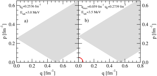
Figure 1: (color online) Regions of the Jacobi momenta $q$ and $p$ values in $(q-p)$ plane which contribute to the breakup reaction ((red) solid line at $E=3.5$ MeV, showing ellipse $\frac{p^{2}}{m}+\frac{3}{4m}q^{2}=\frac{3}{4m}q_{max}^{2}=\frac{3}{4m}q_{0}^{2}+E_{d}$ ) and elastic scattering ($<\Phi^{\prime}|PT|\Phi>$ term) (gray highlighted region) at the incoming nucleon laboratory energy $E=3.0$ and $3.5$ MeV.

It was shown in  [2] (see also  [3, 4] and references therein) that in the treatment based on AGS equation (28) the elastic scattering transition amplitude acquires in the screening limit $R\to\infty$ an infinitely oscillating phase factor and must be renormalized before calculating observables. As a consequence, each term in (32) containing $U\left|{\Phi}\right\rangle$ has to be renormalized. In our approach we solve instead of AGS the 3N Faddeev equation (16) for the $\left\langle{pq\alpha}\right|PT\left|{\Phi}\right\rangle$ states, from which later elastic scattering transition amplitude is calculated. In this way we avoid the main source of the oscillating phase factor described in  [2] and the necessity of renormalization of the elastic scattering amplitude. Additionally, the structure of 3N Faddeev equation guarantees that their solutions inherit properties from the two-nucleon t-matrices providing thus an additional argument that renormalization is redundant. Namely, the properties of t-matrices generated by the screened Coulomb force alone (in the case of partial wave decomposed t-matrices also those generated by a combination of Coulomb and nuclear parts) as well as their screening limits were studied theoretically in the past in numerous papers  [11, 12, 13, 14, 15, 16, 17, 18, 19] and later some of these properties were confirmed numerically in  [10]. The most important finding was that such off-shell t-matrices have a well defined screening limit while the half- and on-shell ones acquire in this limit an infinitely oscillating phase factor. At the same time, the elastic pd scattering amplitude gets contributions of $\left\langle{pq\alpha}\right|T\left|{\Phi}\right\rangle$ states only from the off-shell region of the Jacobi momenta magnitudes $q$ and $p$ in ($q-p$) plane: $\frac{p^{2}}{m}+\frac{3}{4m}q^{2}\neq\frac{3}{4m}q_{max}^{2}=\frac{3}{4m}q_{0}^{2}+E_{d}$, where $m$ is the nucleon mass, $E_{d}$ is the (negative) deuteron binding energy, and $q_{0}$ is the magnitude of the relative pd momentum. That off-shell region of $q-p$ values does not overlap with the ellipse from which half-on-shell contributions to the breakup reaction come. In Fig. 1 we exemplify that off-shell part and the separation of the breakup and elastic scattering regions in the $(q-p)$ plane for the energy of a pd system $E=3.5$ MeV, which is slightly above the breakup threshold and for which both reactions are possible, and at $E=3.0$ MeV, which is below the breakup threshold and for which only elastic scattering is allowed. The fact that elastic pd scattering requires only off-shell solutions of the Faddeev equations and that the off-shell two-nucleon t-matrices have a well defined screening limit is the reason why in our method no renormalization of elastic scattering amplitudes is needed. Contrary to that, the breakup amplitudes acquire the oscillating phase factor originating from half-shell t-matrices.

In order to compare results of two approaches and check that indeed our method does not need the renormalization, we applied our approach at a low proton energy below the breakup threshold, where effects of the pp Coulomb force as well as contributions of different terms to the elastic scattering amplitude are expected to be dominant and where also results of the AGS approach are available at $E=3.0$ MeV  [3]. In Fig. 2 we show our predictions obtained with the AV18 NN potential [20] and $j_{s}3j7$ $\left|{\alpha}\right\rangle$ basis at $3.0$ MeV compared to existing elastic scattering data for the cross section and analyzing powers. The red short dashed line show results obtained with only the first three terms in elastic scattering transition amplitude (18), which is the approximation used also in Ref. [3]. The red solid lines are predictions for neutron-deuteron scattering. It is clear that in this region of energies the Coulomb force effects indeed are large and dominant at all angles as evidenced by comparing the red solid and short dashed lines. It is astonishing how good the overall description of tensor analyzing power data is in spite of their small magnitudes of $\approx 1\%$. The vector analyzing powers $A_{y}$ and $iT_{11}$ are underestimated by theory what is very well known in the literature under the name “low energy analyzing power puzzle”. Even more interesting is the good agreement for practically all shown observables, with the exception of $A_{y}$ and $iT_{11}$, between our $3.0$ MeV results and the predictions based on the AGS approach, as far as it can be judged from Fig. 9 of Ref. [3]. This good agreement strongly supports the statement that both approaches have to provide the same predictions for all observables and that in our approach renormalization of the elastic scattering amplitude is indeed superfluous. The differences for $A_{y}$ and $iT_{11}$ can be very probably traced back to the well known large sensitivity of these observables to the ${}^{3}P_{j}$ components of the NN interaction [9] and different dynamics used by us and in  [3].

In Fig. 2 we show also by dotted blue lines results with the last term in (18) included. It is evident that the term $-\left\langle{\vec{p}\vec{q}~{}}\right|\sum\limits_{\alpha^{\prime}}{\int{\left|{\alpha^{\prime}}\right\rangle\left\langle{\alpha^{\prime}}\right|}}t_{c}^{R}PG_{0}S\sum\limits_{\alpha^{\prime\prime}}{\int{\left|{\alpha^{\prime\prime}}\right\rangle\left\langle{\alpha^{\prime\prime}}\right|}}T\left|{\Phi}\right\rangle$ is significant at low energies and that it deteriorates good description of data obtained with the first three terms. In  [1] it was shown that at energies above $\approx 10$ MeV the contribution of that term to elastic scattering observables is negligible and at $10$ MeV it starts to influence some spin observables. It is thus unavoidable below the breakup threshold to investigate how significant are effects of inclusion of the fourth term $\left\langle{\vec{p}\vec{q}~{}}\right|t_{c}^{R3d}PG_{0}\sum\limits_{\alpha^{\prime}}{\int{\left|{\alpha^{\prime}}\right\rangle\left\langle{\alpha^{\prime}}\right|}}T\left|{\Phi}\right\rangle$ in the elastic scattering transition amplitude. Since the fifth term has a negative sign and contains partial wave contributions to the Coulomb t-matrix whose full 3-dimensional form is contained in the fourth term, one would expect that they would at least partially cancel each other and the inclusion of the fourth term should restore at least partly the good description of data.

The computation of the fourth term with the 3-dimensional Coulomb t-matrix $t_{c}^{R3d}$, can be done according to expressions (D.9), (D.6), and (D.8) of Ref. [5]. It requires integrations over components of two vectors: over vector $\vec{q}$ in (D.9), and over $\vec{p}~{}^{\prime}$ or $\vec{q}_{4}$ in (D.6) or (D.8), respectively. Below the breakup threshold only channels $\alpha\neq\alpha_{d}$ contribute to (D.6). Since below the breakup threshold the decomposition (D.7) is superfluous, (D.8) provides the full contribution from $\alpha_{d}$ channels, obtained by replacing the second part of splitting (D.7) with the left side of (D.7). The contributions from (D.6) and (D.8) must be determined numerically and this is the most time consuming part of the calculations.

In Fig. 2 the indigo crosses show the results obtained with all the terms in (18) included. As expected the fourth and fifth terms cancel each other to a large extent and a good description of data for the cross section and tensor analyzing powers is essentially regained.

To get an idea about the magnitude of the Coulomb force effects for other elastic scattering observables we show in Figs. 3-6 analogous predictions as in Fig. 2 but for selected spin correlations (Fig. 3), proton to proton (Fig. 4), proton to deuteron (Fig. 5), and deuteron to proton (Fig. 6) spin transfer coefficients. The figures reveal a wide spectrum of importance and magnitude of the Coulomb force effects, dependent on the observable. For most of observables the effects are large in a wide range of angles, for example for spin correlations from Fig. 3 and some of spin transfers ($K_{y}^{x}(N-N)$, $K_{y}^{xz}(N-D)$, $K_{zz}^{y}(D-N)$). For some large effects are restricted to forward region of angles below $\approx 90^{o}$ ($K_{x}^{x}(N-N)$, $K_{z}^{x}(N-N)$, $K_{z}^{z}(N-N)$, $K_{x}^{x}(N-D)$, $K_{z}^{x}(N-D)$, $K_{z}^{z}(N-D)$, $K_{x}^{z}(D-N)$, $K_{z}^{z}(D-N)$). There are some interesting cases of observables which for the neutron-deuteron scattering vanish and become nonzero for the proton-deuteron interaction, as for example the nucleon to nucleon spin transfer coefficient $K_{y}^{x}(N-N)$ shown in Fig. 4. These nonzero values are due to a large charge independence breaking of pp and neutron-proton (np) interactions in isospin $t=1$ states, caused by the Coulomb pp force. In our calculations we used the charge dependent AV18 potentials, taking np and pp NN interactions of this model for the pd and nd systems. In all isospin $t=1$ states both total isospins of the 3N system $T=\frac{1}{2}$ and $T=\frac{3}{2}$ were taken into account. Vanishing of the $K_{y}^{x}(n-n)$ for nd scattering shows that the difference between np and pp NN AV18 potentials is too weak to induce nonzero values for this observable.

The very interesting and most important effect seen in all figures is that practically in all cases (large) effects caused by adding the fifth term to the elastic scattering transition amplitude are removed when including simultaneously the fourth term. In consequence, it is needless to account for these terms in elastic scattering amplitude what drastically simplifies and accelerates determination of the Coulomb force effects.

Summarizing, we have shown that the two discussed approaches which enable to include the long range Coulomb force in momentum-space pd scattering calculations by applying a screening method have to provide the same results for all observables. In each method the cancellation between terms containing 3-dimensional and partial wave decomposed Coulomb t-matrices is decisive for establishing workable equations, whose structure is identical to the commonly used equations for neutron-deuteron scattering. Solutions of these equations together with four additional terms, two of which contain the 3-dimensional Coulomb t-matrices, permit one to get the elastic scattering (and breakup) transition amplitudes. In the approach based on the AGS equation it is unavoidable to perform renormalization of the elastic scattering amplitudes before calculating observables. In the approach based on the Faddeev equation such renormalization can be completely avoided. We have shown numerically that the cancellation of last two terms in elastic scattering transition amplitude enables one to determine the pp Coulomb force effects in the pd scattering nearly as easily as to compute observables in neutron-deuteron scattering.

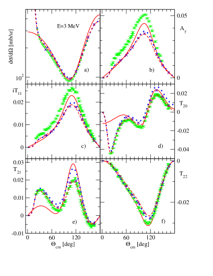
Figure 2: (color online) Comparison of data and predictions for the pd scattering cross section $\frac{d\sigma}{d\Omega}$, proton vector $A_{y}$, deuteron vector $iT_{11}$ and deuteron tensor $T_{20}$, $T_{21}$, $T_{22}$ analyzing powers. They are shown as functions of a c.m. proton scattering angle $\Theta_{cm}$ and were calculated at the incoming proton laboratory energy $E=3.0$ MeV with the approach based on Faddeev equation (16) and transition amplitude (18). The exponentialy screened Coulomb force ($R=40$ fm, $n=4$) and the AV18 potential [20] restricted to the $j\leq 3$ partial waves have been applied. To solve Faddeev equation the set $j_{s}3j7$ of $\left|{\alpha}\right\rangle$ states was used. The red short dashed lines show the results when only the first three terms in (18) are taken into account. The blue dotted lines are predictions when also the fifth term in (18) ($-\left\langle{\vec{p}\vec{q}~{}}\right|{\alpha^{\prime}}\left\rangle\right\langle{\alpha^{\prime}}\left|t_{c}^{R}PG_{0}\right|{\alpha^{\prime\prime}}\left\rangle\right\langle{\alpha^{\prime\prime}}\left|T\right|{\Phi}\left\rangle\right.$) is included. The pure Coulomb term $\left\langle{\Phi^{\prime}}|Pt_{c}P|{\Phi}\right\rangle$ was determined using the screening limit expresion for the off-shell 3-dimensional Coulomb t-matrix (Eq. (19) in Ref. [1]). The indigo crosses show the results with all terms in (18) included. The red solid lines are predictions for nd elastic scattering and green circles represent the pd data from Ref. [21].

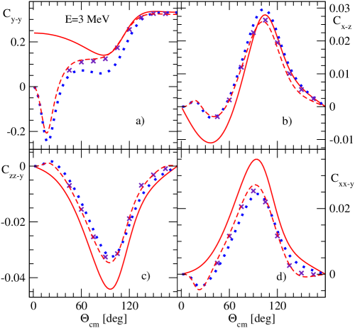
Figure 3: (color online) The same as in Fig. 2 but for selected spin correlation coefficients. For description of lines see Fig. 2.

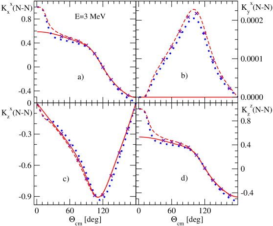
Figure 4: (color online) The same as in Fig. 2 but for selected proton to proton spin transfer coefficients. For description of lines see Fig. 2.

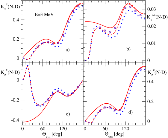
Figure 5: (color online) The same as in Fig. 2 but for selected proton to deuteron spin transfer coefficients. For description of lines see Fig. 2.

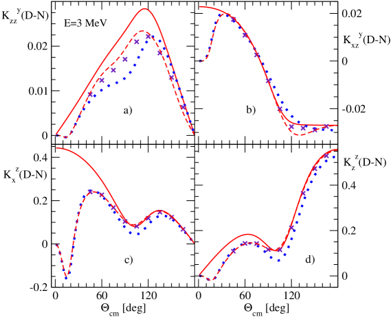
Figure 6: (color online) The same as in Fig. 2 but for selected deuteron to proton spin transfer coefficients. For description of lines see Fig. 2.

References

[1] H. Witała, J. Golak, and R. Skibiński,
arXiv:2310.03433 [nucl.th].
[2] A. Deltuva, arXiv:2311.14605v1 [nucl.th].
[3] A. Deltuva, A. C. Fonseca, and P. U. Sauer,
Phys. Rev. C71, 054005 (2005).
[4] A. Deltuva, A. C. Fonseca, and P. U. Sauer,
Phys. Rev. C72, 054004 (2005).
[5] H. Witała, R. Skibiński, J. Golak,
W. Glöckle,
Eur. Phys. Journal A41, 369 (2009).
[6] H. Witała, R. Skibiński, J. Golak,
W. Glöckle,
Eur. Phys. Journal A41, 385 (2009).
[7] E. O. Alt, P. Grassberger, W. Sandhas, Nucl. Phys. B2,
167 (1967).
[8] W. Glöckle, The Quantum Mechanical Few-Body Problem,
Springer Verlag 1983.
[9] W. Glöckle, H. Witała, D. Hüber, H. Kamada, J.
Golak, Phys. Rep. 274, 107 (1996).
[10] R. Skibiński, J. Golak, H. Witała, and W.Glöckle,
Eur. Phys. Journal A40, 215 (2009).
[11] E. O. Alt, W. Sandhas, and H. Ziegelmann, Phys. Rev. C
17, 1981 (1978).
[12] J.C.Y. Chen and A.C. Chen,
in Advances of Atomic and Molecular Physics,
edited by D. R. Bates and J. Estermann ( Academic, New York, 1972), Vol. 8.
[13] L. P. Kok, H. van Haeringen, P
hys. Rev. C21, 512 (1980).
[14] W.F. Ford, Phys. Rev. 133, B1616 (1964).
[15] W.F. Ford, J. Math. Phys. 7, 626 (1966).
[16] J.R. Taylor, Nuovo Cimento B23, 313 (1974).
[17] M.D. Semon and J.R. Taylor,
Nuovo Cimento A26, 48 (1975).
[18] L. P. Kok, H. van Haeringen,
Phys. Rev. Lett. 46, 1257 (1981).
[19] H. van Haeringen, Charged Particle Interactions,
Theory and Formulas, (Coulomb Press, Leyden, 1985).
[20] R. B. Wiringa, V. G. J. Stoks, R. Schiavilla,
Phys. Rev. C51, 38 (1995).
[21] S. Shimizu et al., Phys. Rev. C 52,
1193 (1995).