Abstract

We study autoequivalences of $D^{b}Coh(X)$ associated to B-brane transport around loops in the stringy Kähler moduli of $X$. We consider the case of $X$ being certain resolutions of determinantal varieties embedded in $\mathbb{P}^{d}\times G(k,n)$. Such resolutions have been modeled, in general, by nonabelian gauged linear sigma models (GLSM). We use the GLSM construction to determine the window categories associated with B-brane transport between different geometric phases using the machinery of grade restriction rule and the hemisphere partition function. In the family of examples analyzed the monodromies around phase boundaries enjoy the interpretation as loop inside link complements. We exploit this interpretation to find a decomposition of autoequivalences into simpler spherical functors and we illustrate this in two examples of Calabi-Yau 3-folds $X$, modeled by an abelian and nonabelian GLSM respectively. In additon we also determine explicitly the action of the autoequivalences on the Grothendieck group $K(X)$ (or equivalently, B-brane charges).

1 Introduction

The study of derived equivalences or equivalences between triangulated categories using gauged linear sigma models [1] (GLSM) is already a well established subject in physics and mathematics [2, 3, 4, 5]. In the present work we proposed the analysis of autoequivalences of derived categories $D^{b}Coh(X)$ of coherent sheaves of Calabi-Yau (CY) varieties $X$ that are given by resolutions of determinantal varieties. The GLSMs having a geometric phase corresponding to a NLSM on $X$ where constructed and their defomation moduli space throughly analyzed in [6]. In particular, their stringy Kähler moduli $\mathcal{M}_{K}(X)$ was completely determined for an extensive family of examples. We will focus on the families termed linear PAX models in [6], which we review in section 2. Let us mention the main characteristics of these models, some of them that encompasses the main novelties of our analysis:

1. The CY variety $X$ is presented as a non-complete intersection inside the space $\mathbb{P}^{n(n-k)-1}\times G(n-k,n)$. Therefore, standard techniques, for example, to determine $\mathcal{M}_{K}(X)$, such as the ones coming from mirror symmetry do not apply generically in these examples.

2. The GLSM realizing $X$ has gauge group $G=U(1)\times U(n-k)$. Therefore $\mathrm{dim}\mathcal{M}_{K}(X)=2$ and it has shown to have three geometric phases [6] denoted by $X_{A}$, $X_{A^{T}}$ and $Y_{A}$

The B-branes of the GLSM are, in part, specified by a representation $\rho_{M}:G\rightarrow GL(M,\mathbb{C})$, whose weights are constrained by the grade restriction rule at the different phase boundaries [7]. We will first focus on determining the window categories defined by the grade restriction rules at the $(X_{A},X_{A^{T}})$ phase boundary and at the $(X_{A},Y_{A})$ phase boundary which we call $X$ and $Y$ phase boundary, respectively. Denoting the weights of $\rho_{M}$ as $q^{0}$ for the $U(1)$ factor and $q^{\alpha}$, $\alpha=1,\ldots,n-k$ for the $U(n-k)$ factor, the window category $\mathbb{W}_{Y}(\theta_{0})$ at the $Y$ boundary is determined (see section 4) to be given by

$$-\frac{n(n-k)}{2}<\frac{\theta_{0}}{2\pi}+q^{0}<\frac{n(n-k)}{2},$$ (1.1)

and the window category $\mathbb{W}_{X}(\theta_{1})$ at the $X$ boundary is determined by the hypercube

$$-\frac{k+1}{2}<\frac{\theta_{1}}{2\pi}+q^{\alpha}<\frac{k+1}{2},\qquad\text{For all \ }\alpha$$ (1.2)

As an application/check of these results, we compute the monodromy around the phase boundaries in two specific examples, one is an abelian model, the determinantal quintic $X_{5}\subset\mathbb{P}^{4}\times\mathbb{P}^{4}$ and the Gulliksen-Negard (GN) determinantal variety $X_{GN}\subset\mathbb{P}^{7}\times G(2,4)$, both CY 3-folds. In the case of $X_{5}$, the computation is standard and can be performed using the already known techniques of [7], so, it serves as a good check for our general results. We find the that the autoequivalence $T_{X}\in\mathrm{Aut}(D^{b}Coh(X_{5}))$ associated to the monodromy around the $X$ phase boundary is given by:

$$T_{X}=\mathcal{D}_{x}^{-5}(\mathcal{D}_{x}T_{\mathcal{O}_{X_{5}}})^{5}\qquad\mathcal{D}_{x}:=-\otimes\mathcal{O}_{X_{5}}(1,0)$$ (1.3)

and the autoequivalence $T_{Y}$ corresponding to the monodromy around the $Y$ phase boundary:

$$T_{Y}=\mathcal{D}_{y}^{-5}(\mathcal{D}_{y}T_{\mathcal{O}_{X_{5}}})^{5}\qquad\mathcal{D}_{y}:=-\otimes\mathcal{O}_{X_{5}}(0,-1)$$ (1.4)

where $T_{E}$ denotes the spherical twist with respect to the object $E$. Likewise for $X_{GN}$ we obtain

$$T_{X}=-\otimes\mathcal{O}_{X_{GN}}(-4,0)$$ (1.5)

and

$$T_{Y}=\mathcal{D}^{-3}(T_{\mathcal{O}_{X_{GN}}}\mathcal{D})^{3}T_{S_{X}}T_{\mathcal{O}_{X}}\mathcal{D}T_{S_{X}}\mathcal{D}^{-1}$$ (1.6)

where in this case $\mathcal{D}:=-\otimes\mathcal{O}_{X_{GN}}(0,-1)$ and $\mathcal{O}_{X_{GN}}(0,-1)$ stands for $\mathcal{O}_{X_{GN}}$ twisted by $\mathrm{det}^{-1}S_{X}$ where $S_{X}$ stands for the tautological subbundle of $G(2,4)$ pulled back to $X_{GN}$. The expressions for $T_{X}$ in both examples are directly found from functors mapping between the windows. On the other hand, the expression for $T_{Y}$ is found in an analogous way, however, its decomposition in terms of simpler spherical functors is found after a careful analysis of the fundamental group $\pi_{1}(\mathcal{M}_{K}(X))$ around the $Y$ phase boundary, as it was done in [10] for some specific abelian models (see section 5). A similar decomposition in principle exists for $T_{X}$ as well but we can only determine it in the case of $X_{5}$, being $\pi_{1}(\mathcal{M}_{K}(X_{GN}))$ near the $X$ boundary too technically challenging to analyze.

The paper is organized as follows. In section 2 we review the general aspects about GLSMs for determinantal varieties from [6] and in particular the ones for linear PAX models as well as the two working examples $X_{5}$ and $X_{GN}$. In section 3 after reviewing the construction of B-branes and the hemisphere partition function $Z_{\mathcal{B}}(t)$ (3.4) for GLSMs, following mostly [7, 5, 11] we compute explicitly the B-branes corresponding to generators of $D^{b}Coh(X_{A})$ and check against their central charges (via the hemisphere partition function) that they indeed give the correct geometric content. We present explicit expressions for the central charges in the $X_{A}$ phase. In 4 we compute the grade restriction rule determining the window categories at the $X$ and $Y$ phase boundaries and the empty branes at the different phases that will be used to compute monodromies later on. In 5 we use the window categories and empty branes to compute the monodromies as autoequivalences acting on $D^{b}Coh(X_{A})$ and using the B-brane central charges from 3, we compute the matrices corresponding to $T_{X}$ and $T_{Y}$ as acting on the basis of the K-theory/brane charges.

2 GLSMs for Determinantal Varieties

In this section we review the construction of GLSMs for certain determinantal CYs. We will focus on the construction of a class of $U(1)\times U(k)$ gauge theories, termed ’PAX models’ in [6]. In particular we will be interested in linear PAX models (defined below). These models includes our main working examples, the determinantal quintic [12, 13] in ${{\mathbb{P}}}^{4}$ and the Gullinksen-Negard (GN) CY [14] (or more precisely, its resolution) in ${{\mathbb{P}}}^{7}\times G(2,4)$.

2.1 Determinantal Varieties and PAX Model

Let $B$ be a compact algebraic variety of dimension $d$, and two holomorphic vector bundles $\mathcal{E}$, $\mathcal{F}$ over $B$ of rank $n$ and $m$ respectively. Without loss of generality, assume $m\leq n$. In addition, consider a holomorphic section $A$ of the bundle $\operatorname{Hom}(\mathcal{E},\mathcal{F})$. Then, the determinantal variety $Z(A,k)$, for $0\leq k<m$ is defined by:

$$Z(A,k)=\{\phi\in B\ |\ \operatorname{rank}A(\phi)\leq k\},$$ (2.1)

$Z(A,k)$ is an algebraic variety, with $I(Z(A,k))$ the ideal generated by all $(k+1)\times(k+1)$ minors of $A$. Since, in general, the number of $(k+1)\times(k+1)$ minors generally exceeds the codimension of $Z(A,k)$ in $B$, which is $(m-k)(n-k)$, determinantal varieties are generically non-complete intersections. When $\operatorname{Hom}(\mathcal{E},\mathcal{F})$ is generated by global sections, all singularities on $Z(A,k)$ arise only at $Z(A,k-1)\subset Z(A,k)$, or at singularities induced from $B$.

Denote $B_{\mathcal{E},k}$ the fibration of the (relative) Grassmannian of $k$-planes plane in the fibers of $\mathcal{E}$ i.e. the fiber of $B_{\mathcal{E},k}$ over $\phi\in B$ is given by $G(k,\mathcal{E}_{\phi})$:

(2.2)

We can use $B_{\mathcal{E},n-k}$ (with fibers $G(n-k,\mathcal{E})$) to construct a desingularization $\tilde{Z}(A,k)$ of $Z(A,k)$ through an incidence correspondence [15]:

$$X_{A}:=\tilde{Z}(A,k)=\{p\in B_{\mathcal{E},n-k}\ |\ A(\pi(p))\circ\pi^{-1}(p)=0\},$$ (2.3)

then, the incidence correspondence $X_{A}$ resolves the singularities located at $Z(A,k-1)\subset Z(A,k)$ and $X_{A}$ is birational to $Z(A,k)$.

Consider now $B_{\mathcal{E}^{\vee},k}$ (with fibers $Gr(k,\mathcal{E}^{\vee})$) where $\mathcal{E}^{\vee}$ denotes the dual bundle to $\mathcal{E}$ and let $\mathcal{U}$ be the rank $k$ sub-bundle and $\mathcal{Q}$ the rank $n-k$ quotient sub-bundle on $B_{\mathcal{E}^{\vee},k}$, which restrict to the corresponding bundles on $Gr(k,\mathcal{E}^{\vee})$. Define then the bundle $\mathcal{X}$ by

$$\mathcal{X}:=(\pi^{*}\mathcal{E}^{\vee}/\mathcal{U})\otimes\pi^{*}\mathcal{F}\cong\operatorname{Hom}(\mathcal{Q}^{\vee},\pi^{*}\mathcal{F}),$$ (2.4)

which has a global holomorphic section $\tilde{A}$ induced from $A$ :

$$\tilde{A}:B_{\mathcal{E}^{\vee},k}\rightarrow\mathcal{Q}\otimes\pi^{*}\mathcal{F},\quad\tilde{A}=f\circ\pi^{*}A.$$ (2.5)

It is then straightforward to show that $X_{A}$ is isomorphic to the variety $X_{\tilde{A}}$ given by the zeroes of $\tilde{A}$ in $B_{\mathcal{E}^{\vee},k}$ [6]. That is

$$X_{\tilde{A}}=\{\tilde{A}=0\}\cap B_{\mathcal{E}^{\vee},k}\cong X_{A}$$ (2.6)

The advantage of having $X_{\tilde{A}}$ is that, it is a complete intersection, hence, topological invariants can be computed straightforwadly in $X_{\tilde{A}}$ and then related to the topological invariants in $X_{A}$ using the isomorphism. For instance, the total Chern class of $X_{\tilde{A}}$ is givne by

$$c(X_{\tilde{A}})=\frac{c(B_{\mathcal{E}^{\vee},k})}{c(\mathcal{X})}.$$ (2.7)

In particular,

$$c_{1}(X_{\tilde{A}})= c_{1}(B_{\mathcal{E}^{\vee},k})-c_{1}(\mathcal{X})$$ (2.8)

$$=\pi^{*}c_{1}(B)-(m-k)\pi^{*}c_{1}(\mathcal{E}^{\vee})-(n-k)\pi^{*}c_{1}(\mathcal{F})-(n-m)c_{1}(\mathcal{U}).$$

The Euler characteristic $\chi(X_{\tilde{A}})$ can be evaluated by

$$\chi(X_{\tilde{A}})=\int_{X_{\tilde{A}}}c_{top}(X_{\tilde{A}})=\int_{B_{\mathcal{E}^{\vee},k}}c_{top}(\mathcal{X})\wedge c_{top}(X_{\tilde{A}}).$$ (2.9)

Furthermore, the intersection numbers $I(\gamma_{k_{1}},\cdots,\gamma_{k_{s}})$ for cohomology classes $\gamma_{k}\in H^{ev}(X_{\tilde{A}},{{\mathbb{Z}}})$ induced from $B_{\mathcal{E}^{\vee},k}$ are computed by

$$I(\gamma_{k_{1}},\cdots,\gamma_{k_{s}})=\int_{X_{\tilde{A}}}\gamma_{k_{1}}\wedge\cdots\wedge\gamma_{k_{s}}=\int_{B_{\mathcal{E}^{\vee},k}}c_{top}(\mathcal{X})\wedge\gamma_{k_{1}}\wedge\cdots\wedge\gamma_{k_{s}}.$$ (2.10)

In the followig we will work with particular familes of smooth determinantal varieties $X_{A}$, that were termed ’PAX models’ in [6]. These families are also called linear determinantal varietes and arise whenever $\mathcal{E}$ takes the form ($\mathcal{F}$ remains arbitrary)

$$\mathcal{E}=\mathcal{L}\otimes\mathcal{O}_{B}^{\oplus n}$$ (2.11)

where $\mathcal{L}$ is a line bundle. In such case, the fibration becomes trivial:

$$B_{\mathcal{E}^{\vee},k}\cong B\times G(k,n)$$ (2.12)

and the variety $X_{A}$ can be written as

$$\begin{gathered}X_{A}=\{(\phi,x)\in B\times G(n-k,n)\ |\ A(\phi)x=0\}\end{gathered}$$ (2.13)

For our interest on determinantal Calabi-Yau 3-folds, we require

$$\dim X_{A}=d-(n-k)(m-k)=3,\quad c_{1}(X_{A})=0.$$ (2.14)

Then the dimension of singular loci is $2k-(n+m-2)$. Hence a 3-fold has non-empty singular locus if $n-1=m-1=k$. Otherwise, there is no locus of reduced rank with generic $A$. Furthermore, we will restrict to the case

$$m=n,$$ (2.15)

i.e. $A$ will be a square matrix. Several possible generalizations of these conditions are discussed in [6].

2.2 GLSM Construction

In this subsection we introduce a construction for a GLSM that implements the linear determinantal varieties discussed above. More precisely, here we review the construction of [6] for a linear determinantal variety i.e. a GLSM that has a geometric phase corresponding to a nonlinear sigma model with target space $X_{A}$. In this construction we will restrict to the case that the variety $B$ is a projective space. In general we can consider $B$ to be any toric variety, in a straightforward way. For this purpose, consider the gauge group

$$G=U(1)^{s}\times U(n-k)$$ (2.16)

and matter superfields (chiral superfields) in the following representation of $G$: $\Phi_{a}$, $a=1,\cdots,d+s$ in the trivial representation of $U(n-k)$ and in with weights $Q_{a}$ under $U(1)^{s}$. $P_{i}$, $i=1,\ldots,n$ in the fundamental of $U(n-k)$ and weights $-\mathfrak{q}_{i}$ under $U(1)^{s}$. $X_{i}$, $i=1,\ldots,n$ in the antifundamental of $U(n-k)$ and weights $q_{i}$ under $U(1)^{s}$. Chossing a basis for $U(1)^{s}=U(1)_{1}\times\cdots\times U(1)_{s}$ we can summarize the matter representation in the following table ($l=1,\ldots,s$)

$$\begin{array}[]{c|ccc}&\Phi_{a}&P_{i}&X_{i}\\ \hline\cr U(1)_{l}&Q_{a}^{l}&-\mathfrak{q}_{i}^{l}&-q_{i}^{l}\\ U(n-k)&0&\mathbf{n-k}&\overline{\mathbf{n-k}}\end{array}$$ (2.17)

The matter interact via the $G$-invariant superpotential

$$W=\sum_{i,j=1}^{n}\mathrm{Tr}(P_{i}A(\Phi)^{ij}X_{j}),$$ (2.18)

there the trace is taken over $U(n-k)$ and $A(\Phi)^{ij}$ is homogeneous in $\Phi$, however its degree depends on the particular model. Then, (2.18) is $G$-invariant, provided that

$$\deg_{l}\left(A(\phi)^{ij}\right)=\mathfrak{q}_{i}^{l}+q_{j}^{l},\quad\forall i,j=1,\cdots,n.$$ (2.19)

where $\deg_{l}(f)$ denotes the weight of $f$ under $U(1)_{l}$. In the following we will denote $\phi,x$ and $p$ the lowest components of the superfields $\Phi,X$ and $P$ respectively.

This model was called PAX model in [6] and we will refer in general to these family of models, as such. The anomaly-free $U(1)_{A}$ condition is given by

$$\sum_{a=1}^{d+s}Q_{a}^{l}=(n-k)\deg_{l}\left(\det A(\phi)\right),\quad\forall l=1,\cdots,s.$$ (2.20)

and the central charge of PAX model is given by

$$\hat{c}:=\frac{c}{3}=d-(n-k)^{2}.$$ (2.21)

In [6] these models are shown to correspond to geometric GLSMs for $X_{A}$ and the $c_{1}(X_{A})$ condition to be equivalent to 2.20. In the following subsection we will review a subfamily of these models termed linear PAX models.

2.3 Linear PAX model for Calabi-Yau 3-folds

A linear PAX model is defined by the condition that $A(\Phi)$ is linear in $\Phi$. Therefore we can write

$$A(\Phi)=\sum_{a=1}^{d+s}A^{a}\Phi_{a},\qquad A^{a}\in\mathrm{Mat}_{n\times n}(\mathbb{C}).$$ (2.22)

In the following we will set

$$s=1\qquad Q_{a}=1,$$ (2.23)

then this model corresponds to a two parameter GLSM with a geometric phase corresponding to $X_{A}\subset\mathbb{P}^{d}\times G(n-k,n)$. The condition 2.20 can then be fullfiled with the following choice of matter representations:

$$\begin{array}[]{c|ccc}&\Phi_{a}&P_{i}&X_{i}\\ \hline\cr U(1)&1&-1&0\\ U(n-k)&0&\mathbf{n-k}&\overline{\mathbf{n-k}}\end{array}$$ (2.24)

Recall the FI-theta parameters can be written as $t=\zeta-i\theta$, where [11]

$$t\in\left(\frac{\mathfrak{t}^{\vee}_{\mathbb{C}}}{2\pi i\mathrm{P}}\right)^{W_{G}}\cong\frac{\mathfrak{z}^{\vee}_{\mathbb{C}}}{2\pi i\mathrm{P}^{W_{G}}},$$ (2.25)

here $\mathrm{P}$ denotes the weight lattice, $W_{G}$ the Weyl subgroup of $G$, $\mathfrak{t}$ the Cartan subalgebra of $\mathfrak{g}=\mathrm{Lie}(G)$ and $\mathfrak{z}=\mathrm{Lie}(Z(G))$. In the present case we can choose a basis where the FI-theta parameters for $U(1)$ and $U(n-k)$ can be denoted $t_{0}$ and $t_{1}$ respectively, $t_{\alpha}=\zeta_{\alpha}-i\theta_{\alpha}$, $\alpha=0,1$. The phases of these models are all weakly coupled and were determined in [6] aas we proceed to review. All the phases corresponde to NLSMs whose target space is given by the classical geometry of the Higgs branch, that is

$$X_{\zeta}:=\mu^{-1}(0)/G\cap\{dW^{-1}(0)\}$$ (2.26)

where $\mu:V\rightarrow\mathfrak{g}^{\vee}$ denotes the moment map on the vector space $V$ (whose coordinates are $(\phi,x,p)$). Then, the equations $\mu^{-1}(0)=0$ corresponds to the D-term equations, for each factor of $G$:

$$\begin{gathered}U(1):\quad\sum_{a=1}^{d+1}|\phi_{a}|^{2}-\sum_{i=1}^{n}\mathrm{Tr}(p_{i}p^{\dagger,i})-\zeta_{0}=0\\ U(n-k):\qquad\sum_{i=1}^{n}\left(p_{i}p^{\dagger,i}-x^{\dagger,i}x_{i}\right)-\zeta_{1}\mathbf{1}_{n-k}=0\end{gathered}$$ (2.27)

where $\mathbf{1}_{n-k}$ denotes the identity in $\mathrm{Mat}_{n-k\times n-k}(\mathbb{C})$. The F-term equations $dW^{-1}(0)$ from the superpotental (2.18) become:

$$\sum_{j=1}^{n}(A^{a,ij}\phi_{a})x_{j}=0,\quad\sum_{i=1}^{n}p_{i}(A^{a,ij}\phi_{a})=0,\quad\sum_{i,j=1}^{n}\operatorname{Tr}(p_{i}A^{a,ij}x_{j})=0.$$ (2.28)

The phase space of this result, generically, in three phases[6], see Fig. 1, each corresponding to NLSMs whose target spaces are the smooth determinantal varieties $X_{A}$, $X_{A^{T}}$ and $Y_{A}$ respectively. Explicitly, they are given by ($Y_{A}\cong Y_{A^{T}}$):

$$\zeta_{0}>0,\zeta_{1}<0 : X_{A}=\{(\phi,x)\in{{\mathbb{P}}}^{d}\times Gr(n-k,n)\ |\ A(\phi)^{ij}x_{j}=0\},$$

$$\zeta_{0}+(n-k)\zeta_{1}>0,\zeta_{1}>0 : X_{A^{T}}=\{(\phi,p)\in{{\mathbb{P}}}^{d}\times Gr(n-k,n)\ |\ A(\phi)^{ij}p_{i}=0\},$$

$$\zeta_{0}+(n-k)\zeta_{1}<0,\zeta_{0}<0 : Y_{A}=\{(p,x)\in{{\mathbb{P}}}(S^{\oplus n})\rightarrow Gr(n-k,n)\ |\ \operatorname{Tr}(p_{i}A^{a,ij}x_{j})=0\}.$$

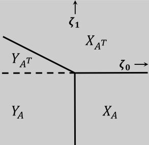
Figure 1: Classical moduli space for linear PAX model. The phase boundary between $Y_{A}$ and $Y_{A^{T}}$ only exists for $\lfloor\sqrt{nk-1}\rfloor\geq k+1$ and $n-k\geq 2$, thus is absent in our explicit examples.

The classical phase boundaries get quantum corrected because of the existence of mixed Coulomb-Higgs mixed branches where the theory breaks down. The loci where these branches occur is a hypersurface (which can have multiple components) in the FI-theta space [1], usually called simply the discriminant of the GLSM. When projected to the $\zeta$-plane (i.e. the FI space), it asymptotically coincides with the classical phase boundaries (up to possibly a constant shift). These descriminants where computed for abelian models in [1, 16] and for nonabelian models in [17]. The nonabelian case is much less straightforward but there is strong evidence [18] supporting the discriminat of PAX models, computed in [6]. Set $q_{\alpha}:=\exp(-t_{\alpha})$ then the discriminant is decribed by the (reducible) parametrized curve[6]

$$(q_{0}(\xi),q_{1}(\xi))=\left((-1)^{n(n-k)}\prod_{\alpha=1}^{n-k}\frac{(1+\omega^{n_{\alpha}}\xi)^{n}}{\xi^{n}},\xi^{n}\right),$$ (2.29)

where $\omega:=e^{2\pi i/n}$, $n_{\alpha}\neq n_{\beta}$ for $\alpha\neq\beta=1,\cdots,n-k$.

Imposing $X_{A}$ to be a CY threefold restricts $(k,n)$ to be

$$(k,n)=(4,5),\ (2,4),\ (1,5)$$ (2.30)

embedded in ${{\mathbb{P}}}^{4}\times{{\mathbb{P}}}^{4}$, ${{\mathbb{P}}}^{7}\times G(2,4)$ and ${{\mathbb{P}}}^{19}\times{{\mathbb{P}}}^{4}$ respectively. The last one is isomorphic to the first one by Seiberg-like duality [19]. Thus $(4,5)$ and $(2,4)$ will serve as the main examples for this paper, which we proceed to analyze their GLSMs in detail in the following subsection.

2.3.1 Determinantal quintic in ${{\mathbb{P}}}^{4}$

This model corresponds to $(k,n)=(4,5)$ and is an abelian GLSM, whose matter content and vector R-charges $U(1)_{R}$ are summarized in the following table:

$$\begin{array}[]{c|ccc}&\Phi_{a}&P_{i}&X_{i}\\ \hline\cr U(1)_{0}&1&-1&0\\ U(1)_{1}&0&1&-1\\ U(1)_{R}&2(1-\epsilon-\delta)&2\epsilon&2\delta\end{array}$$ (2.31)

for $a,i,j=1,\cdots,5$ and $2\epsilon,2\delta\in[0,2)$. Its classical Higgs branch is given by

$$\begin{gathered}X_{A}=\quad\{(\phi,x)\in{{\mathbb{P}}}^{4}\times{{\mathbb{P}}}^{4}\ |\ A(\phi)_{i}\cdot x=0\}\\ X_{A^{T}}=\quad\{(\phi,p)\in{{\mathbb{P}}}^{4}\times{{\mathbb{P}}}^{4}\ |\ p\cdot A(\phi)^{j}=0\}\\ Y_{A}=\quad\{(p,x)\in{{\mathbb{P}}}(\mathcal{O}(-1)^{\oplus 5})\rightarrow{{\mathbb{P}}}^{4}\ |\ p\cdot A^{a}\cdot x=0\},\end{gathered}$$ (2.32)

the variety $X_{A}$ corresponds to the resolved determinantal quintic studied in [20, 21]. Passing through each phase boundary rcorresponds to a flop transition between geometries of both sides.

The determinantal variety $Z(A,4)\subset{{\mathbb{P}}}^{4}$ generically has isolated singular nodal points. This can be verified by the Thom-Porteus formula. In this case $\mathcal{E}=\mathcal{O}^{\oplus 5}$, $\mathcal{F}=\mathcal{O}(1)^{\oplus 5}$, then the cohomology class of the singular loci is given by

$$[Z(A,3)]=\left|\begin{array}[]{cc}c_{2}(\mathcal{F})&c_{3}(\mathcal{F})\\ c_{1}(\mathcal{F})&c_{2}(\mathcal{F})\end{array}\right|=100H^{4}-50H^{4}=50H^{4},$$ (2.33)

where $H$ denotes the hyperplane class of ${{\mathbb{P}}}^{4}$. Therefore, $Z(A,3)$ is generically composed of $50$ singular nodal points. Using the intersection formulae (2.10), one can determine the topological data of $X_{A}$ to be

$$\begin{gathered}\chi(X_{A})=-100\quad c_{2}(X_{A})\cdot H=50\quad c_{2}(X_{A})\cdot\varsigma_{1}=50\\ H^{3}=5\quad H^{2}\cdot\varsigma_{1}=10\quad H\cdot\varsigma_{1}^{2}=10\quad\varsigma_{1}^{3}=5\end{gathered}$$ (2.34)

where $\varsigma_{1}$ denotes the hyperplane class of the Grassmannian $G(1,5)\cong{{\mathbb{P}}}^{4}$. Then we can compute the Hodge numbers of $X_{A}$ to be $(h^{1,1},h^{2,1})=(2,52)$. In particular, positive Kahler cone generators $H$ and $\varsigma_{1}$ are symptotically identified with $\zeta_{0}+\zeta_{1}$ and $\zeta_{1}$ in $X_{A^{T}}$, and $\zeta_{0}$ and $-\zeta_{1}$ in $X_{A}$.

The discriminant in FI parameter space is given by

$$\Delta:\quad(q_{0},q_{1})=\left(-\frac{(1+\xi)^{5}}{\xi^{5}},\xi^{5}\right),$$ (2.35)

which exactly match the result from mirror symmetry [22]:

$$\Delta:\quad(u+v+w)^{5}-5^{4}uvw(u+v+w)^{2}+5^{5}uvw(uv+vw+wu)=0\subset{{\mathbb{P}}}^{2}$$ (2.36)

where we identify $[u,v,w]=[q_{1},q_{0}q_{1},1]\in{{\mathbb{P}}}^{2}$ in the $X_{A^{T}}$ phase and $[u,v,w]=[1,q_{0},q_{1}^{-1}]$ in the $X_{A}$ phase. This identification also matches the FI parameters for generators on each phase. Furtherly, three large volume points corresponding to classical phases are given by

$$u=v=0,\quad v=w=0,\quad w=u=0.$$ (2.37)

The full moduli space is illustrated in Fig.2. $\Delta$ intersects with the divisors $\{w=0\}$, $\{u=0\}$ and $\{v=0\}$ at the points $[1:-1:0]$, $[0:1:-1]$ and $[1:0:-1]$, respectively. All intersections are tangential and of of degree 5.

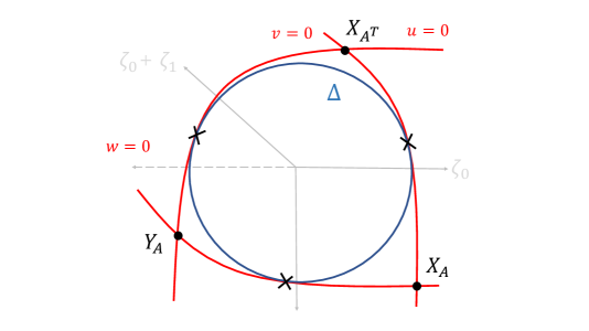
Figure 2: Moduli space for determinantal quintic

2.3.2 GN Calabi-Yau in ${{\mathbb{P}}}^{7}$

This model is a two parameter non-abelian GLSM whose gauge gorup is $G=U(1)\times U(2)$ and with matter content

$$\begin{array}[]{c|ccc}&\Phi_{a}&P_{i}&X_{i}\\ \hline\cr U(1)&1&-1&0\\ U(2)&0&\mathbf{2}&\overline{\mathbf{2}}\\ U(1)_{R}&2(1-\epsilon-\delta)&2\epsilon&2\delta\end{array}$$ (2.38)

for $a=1,\cdots,8$, $i=1,\cdots,4$. The Higgs branch geometries are given by

$$\begin{gathered}X_{A}:\quad\{(\phi,x)\in{{\mathbb{P}}}^{7}\times Gr(2,4)\ |\ A(\phi)_{i}\cdot x^{\alpha}=0\}\\ X_{A^{T}}:\quad\{(\phi,p)\in{{\mathbb{P}}}^{7}\times Gr(2,4)\ |\ p_{\alpha}\cdot A(\phi)^{j}=0\}\\ Y_{A}:\quad\{(p,x)\in{{\mathbb{P}}}(S^{\oplus 4})\rightarrow Gr(2,4)\ |\ p\cdot A^{a}\cdot x=0\}\end{gathered}$$ (2.39)

The geometry of $X_{A}$ is an incidence correspondence for $Z(A,2)$ as

$$Z(A,2)=\{\phi\in{{\mathbb{P}}}^{7}\ |\ \operatorname{rank}(A(\phi))\leq 2\},$$ (2.40)

with topological data

$$\begin{gathered}\chi(X_{A})=-64\quad c_{2}(X_{A})\cdot H=56\quad c_{2}(X_{A})\cdot\varsigma_{1}=56\\ H^{3}=20\quad H^{2}\cdot\varsigma_{1}=20\quad H\cdot\varsigma_{1}^{2}=16\quad\varsigma_{1}^{3}=8\end{gathered}$$ (2.41)

where hyperplane classes are $H$ of ${{\mathbb{P}}}^{7}$ and Schubert class $\varsigma_{1}=c_{1}(Q)$ of $Gr(2,4)$, asymptotically correspond to $\zeta_{0}+2\zeta_{1}$ and $\zeta_{1}$ in $X_{A^{T}}$, and $\zeta_{0}$ and $-\zeta_{1}$ in $X_{A}$. The resulting number $(h^{1,1},h^{2,1})=(2,34)$ matches the result in [23]. Note that Gulliksen and Negård first implicitly described this particular CY 3-fold in terms of a resolution of the corresponding ideal sheaf [14]. The variety was analyzed as a determinantal variety in [23],[24].

Similar analysis shows that $X_{A}$ is the resolution of desingularized variety $Z(\mathcal{A},7)$, for

$$Z(\mathcal{A},7)=\{x\in Gr(2,4)\ |\ \operatorname{rank}\mathcal{A}\leq 7\}$$ (2.42)

in term of $8\times 8$ matrix $\mathcal{A}=A^{a}_{i}\cdot x_{\alpha}$. It has generically 56 nodal points, and the Kähler parameter $2\varsigma_{1}-H$ in $X_{A}$ measures the volume of the 56 blown-up ${{\mathbb{P}}}^{1}$s.

The descriminant from GLSM is given by curves

$$\begin{gathered}\Delta_{1}:\quad(1+w)^{4}-2z(1-6w+w^{2})+z^{2}=0\\ \Delta_{2}:\quad-(1+w)^{8}+4z(1+34w+w^{2})(1+w)^{4}-2z^{2}(3-372w+1298w^{2}-372w^{3}+3w^{4})\\ +4z^{3}(1+34w+w^{2})-z^{4}=0\end{gathered}$$ (2.43)

in where $(w,z)$ should be identified to $(q_{1},q_{0}q_{1}^{2})$ for $X_{A^{T}}$ and to $(q_{1}^{-1},q_{0})$ for $X_{A}$ according to Kähler parameters. Then the moduli structure is symmetric under $q_{1}\mapsto q_{1}^{-1}$. However the full structure of moduli is not known. The moduli structure for $X_{A}$ is illustrated in Fig.3. Note that $\Delta_{1},\Delta_{2}$ intersects divisors at $(z,w)=(0,-1)$ tangentially of degree $4,8$, and at $(1,0)$ of degree $2,4$ respectively.

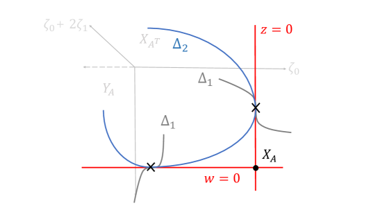
Figure 3: Moduli space for GN Calabi-Yau around $X_{A}$. The $X_{A^{T}}$ side is identical.

The mirror family for this CY is not known, however, its GLSM predicts that the mirror family contains three large complex structure points characterized by maximal unipotent monodromy, and it has a discriminant locus consisting of the two rational curves in (2.43), and boundary divisors associated to the FI parameters tending to infinity.

3 B-branes and their central charges for determinantal varieties

In this section we will review the construction of B-branes on GLSMs from [7, 5] and their central charges as defined in [5]. Afterwards we will apply these results to the specific case of the determinantl quintic and the GN CY defined in section 2.

3.1 B-branes in GLSMs

B-branes on GLSM are defined as boundary conditions that preserve the B-type subset of the $\mathcal{N}=(2,2)$ supersymmetry. Namely if the left and right moving supercharges are denoted $\mathbf{Q}_{-},\overline{\mathbf{Q}}_{-}$ and $\mathbf{Q}_{+},\overline{\mathbf{Q}}_{+}$ respectively, the B-type supersymmetry is spanned by the supercharges $\mathbf{Q}_{B}:=\overline{\mathbf{Q}}_{+}+\overline{\mathbf{Q}}_{-}$ and its charge conjugate $\mathbf{Q}^{{\dagger}}_{B}:=\mathbf{Q}_{+}+\mathbf{Q}_{-}$. In general a GLSM involves chiral and twisted chiral fields, denote them collectively as $\phi$, (taking values in $V\cong\mathbb{C}^{N}$) and $\sigma$ (taking values in $\mathfrak{t}_{\mathbb{C}}$), respectively. One has to define boundary conditions for both types of fields, when dealing with B-branes [7, 5]. The boundary conditions for the chirals $\phi$, transforming on a representation $\rho_{m}:G\rightarrow GL(V)$ and $R:U(1)_{R}\rightarrow GL(V)$ of the gauge group and (vector) R-charge respectively, will involve the superpotential $W\in(\mathrm{Sym}V^{\vee})^{G}$. These boundary conditions are algebraic. We will label them by $\mathcal{B}:=(M,\rho_{M},R_{M},\mathbf{T})$, where the elements in this 4-tuple are defined as:

• Chan-Paton vector space: a $\mathbb{Z}_{2}$-graded, finite dimensional free $\mathrm{Sym}(V^{\vee})$ module denoted by $M=M_{0}\oplus M_{1}$.

• Boundary gauge and (vector) R-charge representation: $\rho_{M}:G\rightarrow GL(M)$, and $R_{M}:U(1)_{R}\rightarrow GL(M)$ are a pair of commuting and $\mathbb{Z}_{2}$-even representations, where the weights of $R_{M}$ are allowed to be real.

• Matrix factorization of $W$: Also known as the tachyon profile, a $\mathbb{Z}_{2}$-odd endomorphism $\mathbf{T}\in\mathrm{End}^{1}_{\mathrm{Sym}(V^{\vee})}(M)$ satisfying $\mathbf{T}^{2}=W\cdot\mathrm{id}_{M}$.

The group actions $\rho_{M}$ and $R_{M}$ must be compatible with $\rho_{m}$ and $R$, i.e. for all $\lambda\in U(1)_{R}$ and $g\in G$ the identities

$$R_{M}(\lambda)\mathbf{T}(R(\lambda)\phi)R_{M}(\lambda)^{-1} =\lambda\mathbf{T}(\phi),$$ (3.1)

$$\rho_{M}(g)^{-1}\mathbf{T}(\rho_{m}(g)\cdot\phi)\rho_{M}(g) =\mathbf{T}(\phi)$$

must hold. Denote the weights of $\rho_{m}$ as $Q_{j}:\mathfrak{t}^{\vee}\rightarrow\mathbb{R}$ and the weights of $R$ as $R_{j}\in\mathbb{R}$ for $j=1\ldots,N=\mathrm{dim}_{\mathbb{C}}V$. Define the collection of hyperplanes $\mathcal{H}\subset\mathfrak{t}_{\mathbb{C}}$ by

$$\mathcal{H}=\bigcup_{j=1}^{N}\bigcup_{n\in\mathbb{Z}_{\geq 0}}\left\{\sigma\in\mathfrak{t}_{\mathbb{C}}\Big{|}Q_{j}(\sigma)-i\frac{R_{j}}{2}-in=0\right\}$$ (3.2)

The other piece of data that we need to fully define the B-brane are the boundary conditions for the twisted chirals. That is, the specification of a profile $L_{t}$ (denoted to emphasize, in general, it may depend on $t$) for the zero modes of $\sigma\in\mathfrak{t}_{\mathbb{C}}$. $L_{t}$ corresponds to a gauge-invariant middle-dimensional subvariety $L_{t}\subset\mathfrak{g}_{\mathbb{C}}\setminus\mathcal{H}$ of the complexified Lie algebra of $G$ or equivalently its intersection $L_{t}\subset\mathfrak{t}_{\mathbb{C}}\setminus\mathcal{H}$ invariant under the action of the Weyl group $W_{G}\subset G$ [5]. In [5], an admissible contour is defined as a profile $L_{t}$ that is a continuous deformation of the real contour $L_{\mathbb{R}}:=\{\operatorname{Im}\sigma=0|\sigma\in\mathfrak{t}_{\mathbb{C}}\}$, such that the imaginary part of the boundary effective twisted superpotential $\widetilde{W}_{\text{eff},q}:\mathfrak{t}_{\mathbb{C}}\rightarrow\mathbb{C}$

$$\widetilde{W}_{\text{eff},q}(\sigma):=\left(\sum_{\alpha>0}\pm i\pi\,\alpha\cdot\sigma\right)-\left(\sum_{j}(Q_{j}(\sigma))\left(\log\left(\frac{iQ_{j}(\sigma)}{\Lambda}\right)-1\right)\right)-t(\sigma)+2\pi iq(\sigma)$$ (3.3)

approaches $+\infty$ in all asymptotic directions of $L_{t}$ and for all the weights $q\in\mathfrak{t}^{\vee}$ of $\rho_{M}$. Signs in the sum over positive roots $\alpha$ of $G$ depend on the Weyl chamber in which $\operatorname{Re}(\sigma)$ lies.

The GLSM B-branes, are then given by pairs $(\mathcal{B},L_{t})$. These are known to form a category which we denote as $MF_{G}(W)$ which was defined purely in terms of the data $\mathcal{B}$ in [4]. However the category $MF_{G}(W)$ with objects given by pairs $(\mathcal{B},L_{t})$ has its origins on the dynamics of B-branes on GLSMs [5] and it can be reduced to the data $\mathcal{B}$ when we are in a specific phase (and so, the data $L_{t}$ can be dropped), in the IR SCFT. However, in our approach, $L_{t}$ is crucial for deriving the relation between the categories of B-branes at different phases as was used for the derivation of the grade restriction rule in [7, 5] and we will review it in section 4.

3.2 Hemisphere Partition Function and Central Charge of B-branes

The central charge of B-branes (A-branes), for $\mathcal{N}=(2,2)$ theories is defined [29, 30] by the partition function the A-twisted (B-twisted) theory on a disk with an infinitely flat cylinder attached to it and boundary conditions corresponding to a B-brane (A-brane). This coupling of A/B-twist in the bulk of $\mathcal{N}=(2,2)$ theories and B/A-brane boundary conditions is a very natural object to study, for instance in SCFTs [31]. Using supersymmetric localization techniques [5, 27, 28] the central charge for a B-brane $(\mathcal{B},L_{t})\in MF_{G}(W)$ was computed in the context of GLSMs and found to be given by

$$Z_{\mathcal{B}}(t):=\int_{L_{t}\subset\mathfrak{t}_{\mathbb{C}}}d^{l_{G}}\sigma\prod_{\alpha>0}\alpha(\sigma)\sinh(\pi\alpha(\sigma))\prod_{j=1}^{N}\Gamma\left(iQ_{j}(\sigma)+\frac{R_{j}}{2}\right)e^{it(\sigma)}f_{\mathcal{B}}(\sigma).$$ (3.4)

where

$$f_{\mathcal{B}}(\sigma):=\mathrm{tr}_{M}\left(R_{M}(e^{i\pi})\rho_{M}(e^{2\pi\sigma})\right)$$ (3.5)

the symbol $\prod_{\alpha>0}$ denotes the product over the positive roots of $G$ and $l_{G}:=\mathrm{dim}(\mathfrak{t})$. The function (3.4) is conjectured to coincide with the IR central charge as defined by [29], for SCFTs i.e. nonanomalous GLSMs and to be related in a certain limit in the anomalous case (see [5, 11]). Is important to remark that in (3.4) the integration variable is dimensionless since it corresponds to $r\sigma$ (where $r$ is the radius of the hemisphere) but we denoted it $\sigma$ in order not to introduce more notation. In addition, (3.4) has a normalization of the form $C(r\Lambda)^{\frac{\hat{c}}{2}}$ where $\Lambda$ corresponds to the UV cut-off and $C$ is just a numerical constant. We will simply set this factor to a convenient numerical constant (specified in each example) in the following, but in general it should be considered for applications involving anomalous models [11], for instance. We will be concerned in this work only with geometric phases. The central charge for B-branes on NLSMs with a CY target space $X$ takes the form [32, 33, 34]

$$\begin{gathered}Z_{\mathcal{B}}(t)=\int_{X}e^{J}\hat{\Gamma}_{X}\mathrm{ch}(\mathcal{B})+\text{instantons}=:Z^{0}_{\mathcal{B}}(t)+\text{ instantons },\end{gathered}$$ (3.6)

where $J:=B+i\frac{\omega}{2\pi}\in H^{2}(X,\mathbb{C})$, $B\in H^{2}(X,\mathbb{Z})$ is the $B$-field and $\omega\in\mathcal{K}_{X}\subset H^{2}(X,\mathbb{R})$. $\mathcal{K}_{X}$ denotes the Kähler cone of $X$ and the instantons are weighted by

$$\exp\left(2\pi i\int_{\beta}J\right)\qquad\beta\in H_{2}(X,\mathbb{Z})$$ (3.7)

where $\beta$ is an effective curve class. The Gamma class $\hat{\Gamma}_{X}$ is a multiplicative characteristic class, given by

$$\hat{\Gamma}_{X}:=\prod_{j}\Gamma\left(1-\frac{\lambda_{j}}{2\pi i}\right)$$ (3.8)

where $\lambda_{j}$ are the Chern roots of the holomorphic tangent bundle $TX$ of $X$. It satisfies the important property

$$\hat{\Gamma}_{X}\hat{\Gamma}^{*}_{X}=\hat{A}_{X}$$ (3.9)

with $\hat{A}_{X}$ the $\hat{A}$-genus of $X$. For $X$ CY, the $\hat{A}$-genus equals the Todd class $\mathrm{Td}_{X}$. Because of (3.9), we can regard $\hat{\Gamma}_{X}$ as a root of $\hat{A}_{X}$ moreover, this root is not unique and $\hat{\Gamma}_{X}$ is just a particular choice [35], however this choice is different from the one corresponding to the Ramond-Ramond (RR) charge computed in [32, 33, 34]. The choice $\hat{\Gamma}_{X}$ encodes the perturbative corrections to the central charge. Fix $X$ to be a CY 3-fold, then $\hat{\Gamma}_{X}$ is explicitly given by

$$\hat{\Gamma}_{X}=1+\frac{1}{24}c_{2}(X)+\frac{\zeta(3)}{(2\pi i)^{3}}c_{3}(X).$$ (3.10)

Fix a basis $\{J_{\alpha}\}$ of $H^{2}(X,{{\mathbb{C}}})$ and so we can write $J=\kappa_{\alpha}J_{\alpha}$, $\kappa_{\alpha}\in\mathbb{C}$, then we can write explicitly the central charge at the zero-instanton sector for chosen basis of generators of $D^{b}Coh(X)$ given by sheaves, namely

$$\begin{gathered}\begin{aligned} Z^{0}_{\mathcal{O}_{X}}(t)=\frac{1}{3!}c_{\alpha\beta\gamma}\kappa_{\alpha}\kappa_{\beta}\kappa_{\gamma}+c_{\alpha}\kappa_{\alpha}+\frac{\zeta(3)}{(2\pi i)^{3}}\chi(X),\end{aligned}\\ c_{\alpha\beta\gamma}:=\int_{X}J_{\alpha}J_{\beta}J_{\gamma},\quad c_{\alpha}:=\frac{1}{24}\int_{X}c_{2}(X)J_{\alpha},\end{gathered}$$ (3.11)

Similarly, for each generator $J_{\alpha}$ we have a D4-brane $\mathcal{O}_{D_{\alpha}}$ corresponding to the structure sheaf of the divisor $D_{\alpha}$, dual to $J_{\alpha}$, having brane charge

$$Z^{0}_{\mathcal{O}_{D_{\alpha}}}(t)=\frac{1}{2}c_{\alpha\beta\gamma}\kappa_{\beta}\kappa_{\gamma}-\frac{1}{2}c_{\alpha\alpha\beta}\kappa_{\beta}+\frac{1}{6}c_{\alpha\alpha\alpha}+c_{\alpha}.$$ (3.12)

The D2-branes $\mathcal{O}_{C^{\alpha}}$ supported on the curve classes $C^{\alpha}$ have

$$Z^{0}_{\mathcal{O}_{C^{\alpha}}}(t)=\kappa_{\alpha}+1$$ (3.13)

while the D0-brane $\mathcal{O}_{p}$ supported at a point $p\in X$, i.e. the skyscraper sheaf at $p$, is normalized to

$$Z^{0}_{\mathcal{O}_{p}}(t)=1.$$ (3.14)

The lattice of B-brane charges is isomorphic to the Grothendieck group $K_{0}(X)$ of the CY $X$ which is spanned by homological classes of holomorphic vector bundles over $X$[40, 37]. Indeed the central charges $Z:D(X)\rightarrow\mathbb{C}$ factor through $K_{0}(X)$, hence we can always uniquely write the central charge of a B-brane $\mathcal{B}$ as:

$$Z_{\mathcal{B}}=a^{0}Z_{\mathcal{O}_{X}}+a^{\alpha}Z_{\mathcal{O}_{D_{\alpha}}}+a_{\alpha}Z_{\mathcal{E}_{\alpha}}+a_{0}Z_{\mathcal{O}_{P}}=:\left(a^{0},a^{\alpha},a_{\alpha},a_{0}\right),$$ (3.15)

where $a^{0},a^{\alpha},a_{\alpha},a_{0}\in\mathbb{Z}$.

3.3 B-branes and their central charges in linear PAX models and central charges

In this subsection we will perform the explicit evaluation of the (quantum corrected) central charge for the B-branes generating the derived category $D^{b}Coh(X_{A})$ for our choice of examples. Since all the phases are geometric (and weakly coupled) in the linear PAX models, the computations presented in this sections can be carried on in analogous way in other phases. In addition, the linear PAX models we are considering are CY 3-folds and have $h^{1,1}=2$, hence a canonical choice of generators for $D^{b}Coh(X_{A})$ will be chosen to be $\{\mathcal{O}_{X},\mathcal{O}_{D_{\alpha}},\mathcal{E}_{\alpha}\}$, $\alpha=0,1$ where $\mathcal{E}_{\alpha}$ is a twist of $\mathcal{O}_{C^{\alpha}}$. $\mathcal{O}_{C^{\alpha}}$ and $\mathcal{O}_{D_{\alpha}}$ are the structure sheaves of curves and divisors on $X_{A}$, respectively.

The convergence condition can be solved by requiring $\operatorname{Im}\sigma_{0}>0$ and $\operatorname{Im}\sigma_{1,\mathsf{k}}<0$ in the $X_{A}$ phase. Then, an admissible contour $\gamma$ can be taken as

$$\gamma:\quad\left(\sigma_{0},\sigma_{1}\right)=\left(\operatorname{Re}\sigma_{0}+i\left(\operatorname{Re}\sigma_{0}\right)^{2},\operatorname{Re}\sigma_{1,\mathsf{k}}-i\left(\operatorname{Re}\sigma_{1,\mathsf{k}}\right)^{2}\right),\quad\mathsf{k}=1,\ldots,k.$$ (3.16)

Then, in the limit of the R-charge of $\phi$ and $x$ to be zero, and that of $p$ to be $2$ (the exact R-charges at the IR fixed point in the $X_{A}$ phase) the integral (3.4) can be be evaluated by multidimensional residues in a neighbourhood of the poles.

3.3.1 Determinantal quintic in ${{\mathbb{P}}}^{4}$

The hemisphere partition function (3.4) of a B-brane $\mathcal{B}$ is given by

$$Z_{\mathcal{B}}(t)=\frac{1}{(2\pi i)^{8}}\int_{\gamma}d^{2}\sigma e^{it(\sigma)}\Gamma(i\sigma_{0}+1-\epsilon-\delta)^{5}\Gamma(i(\sigma_{1}-\sigma_{0})+\epsilon)^{5}\Gamma(-i\sigma_{1}+\delta)^{5}f_{\mathcal{B}}(\sigma),$$ (3.17)

where we have taken a normalization factor $(2\pi i)^{-8}$. The contour $\gamma$ is chosen so that is admissible in the $X_{A}$ phase. $Z_{\mathcal{B}}(t)$ is convergent, for any $\mathcal{B}$,provided $\operatorname{Im}\sigma_{0}>0$ and $\operatorname{Im}\sigma_{1}<0$, then, is straightforward to show that the following integration contour satisfy all the admissibility conditions:

$$\gamma:\quad\left(\sigma_{0},\sigma_{1}\right)=\left(\operatorname{Re}\sigma_{0}+i\left(\operatorname{Re}\sigma_{0}\right)^{2},\operatorname{Re}\sigma_{1}-i\left(\operatorname{Re}\sigma_{1}\right)^{2}\right).$$ (3.18)

The poles of Gamma functions lies in the families of hyperplanes

$$\mathcal{H}_{1}=\left\{\sigma_{0}=i(k+1-\epsilon-\delta)\right\}_{k=0}^{\infty},\ \mathcal{H}_{2}=\left\{\sigma_{1}=-i(k+\delta)\right\}_{k=0}^{\infty},\ \mathcal{H}_{3}=\left\{\sigma_{1}-\sigma_{0}=i(k+\epsilon)\right\}_{k=0}^{\infty}$$ (3.19)

where $k\in{{\mathbb{Z}}}_{\geq 0}$. The projection of the hyperplanes to the $\mathrm{Im}\sigma$ plane is illustrated in Fig.4. Given $\gamma$, using the prescription of [41, 42], the integral on $Z_{D^{2}}(\mathcal{B})$ can be reduced to an infinite sum of residues. When the FI parameters $\zeta$ are chosen on the chamber of the phase $X_{A}$, this sum is over the the residues of the poles located at $\mathcal{H}_{1}\cap\mathcal{H}_{2}$.

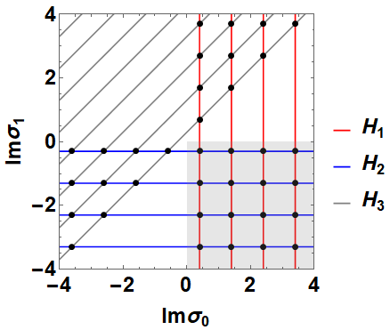
Figure 4: Gamma poles of the determinantal quintic. The admissible contour envelops poles in the lower-right quadrant.

Then the partition function (3.17) has a series expression as a sum over residues of admissible poles:

$$Z_{\mathcal{B}}(t)= \frac{1}{(2\pi i)^{8}}\sum_{n,m=0}^{\infty}\operatorname{Res}_{(z_{0},z_{1})=(n,m)}\left(\frac{\pi}{\sin\pi z_{0}}\right)^{5}\left(\frac{\pi}{\sin\pi z_{1}}\right)^{5}$$ (3.20)

$$\times \frac{\Gamma(z_{0}+z_{1}+1)^{5}}{\Gamma(z_{0}+1)^{5}\Gamma(z_{1}+1)^{5}}e^{-t_{0}z_{0}+t_{1}z_{1}}f_{\mathcal{B}}(iz_{0},-iz_{1}).$$

where we have taken the limit $(\delta,\epsilon)\rightarrow(0,1)$ to set the R-charges to their exact value in the $X_{A}$ phase. Since $\gamma$ is admissible for any element $\mathcal{B}\in MF_{G}(W)$, in the $X_{A}$ phase, in the following we will present a particular choice of representatives $\mathcal{B}$ that flows to our desired set of generators in $D^{b}Coh(X_{A})$. The tachyon profile

$$Q_{\mathcal{O}_{X}(p,q)}:=p_{i}\bar{\eta}^{i}+A(\phi)^{ij}x_{j}\eta_{i},$$ (3.21)

which is conveniently expressed in terms of free fermions $\eta_{i}$, $\bar{\eta}^{i}$ satisfying the Cifford algebra

$$\{\eta_{i},\bar{\eta}^{j}\}=\delta^{j}_{i},\quad\{\bar{\eta}^{i},\bar{\eta}^{j}\}=\{\eta_{i},\eta^{j}\}=0\qquad\text{ \ for all \ }i,j=1,\ldots,5$$ (3.22)

the representations $\rho_{M}$ and $R_{M}$ are uniquely determined by the choice of Clifford vaccum $|p,q\rangle$, on an irreducible representation of the gauge group $U(1)\times U(1)$, satisfying

$$\bar{\eta}^{i}|p,q\rangle=0\text{ \ \ for all \ }i,\qquad\rho_{M}(\lambda_{1},\lambda_{2})|p,q\rangle=\lambda_{1}^{p}\lambda_{2}^{q}|p,q\rangle\qquad R_{M}(\lambda)|p,q\rangle=|p,q\rangle$$ (3.23)

for all $(\lambda_{1},\lambda_{2})\in U(1)\times U(1)$ and $\lambda\in U(1)_{R}$. Then its brane factor $f_{\mathcal{O}_{X}(p,q)}(\sigma)$ can be straightforwardly computed:

$$f_{\mathcal{O}_{X}(p,q)}(\sigma)=\left(1-e^{2\pi(\sigma_{1}-\sigma_{0})}\right)^{5}e^{2\pi(p\sigma_{0}+q\sigma_{1})}.$$ (3.24)

These B-branes RG-flow to the objects $\mathcal{O}_{X_{A}}(p,q)\in D^{b}Coh(X_{A})$. It is possible to choose some subset of the $(p,q)$ pairs such that $\mathcal{O}_{X_{A}}(p,q)$ generate $D^{b}Coh(X_{A})$ but we are not going to use this basis here. The zero instanton sector of the B-brane $Q_{\mathcal{O}_{X}(p,q)}$ is given by

$$Z^{0}_{\mathcal{O}_{X}(p,q)}$$ (3.25)

$$= -\frac{100\zeta(3)}{(2\pi i)^{3}}+\frac{5}{12}(p-q)(5+2(p^{2}-5pq+q^{2}))$$

$$+\left(50+60(p^{2}-4pq+2q^{2})\right)\frac{\kappa_{0}}{24}$$

$$+\left(50+60(2p^{2}-4pq+q^{2})\right)\frac{\kappa_{1}}{24}$$

$$+\frac{5}{2}\left((p-2q)\kappa_{0}^{2}+4(p-q)\kappa_{0}\kappa_{1}+(2p-q)\kappa_{1}^{2}\right)$$

$$+\frac{5}{6}\kappa_{0}^{3}+5\kappa_{0}^{2}\kappa_{1}+5\kappa_{0}\kappa_{1}^{2}+\frac{5}{6}\kappa_{1}^{3},$$

where Kähler parameters are identified with

$$\kappa_{0}=-\frac{t_{0}}{2\pi i}-5/2,\qquad\kappa_{1}=\frac{t_{1}}{2\pi i}-5/2.$$ (3.26)

We remark that the identification (3.26) is only valid asymptotically i.e. it must be understood up to instanton correcions, in general $\kappa_{0}=-\frac{t_{0}}{2\pi i}-5/2+\mathcal{O}(\exp(-t_{0}))$ and likewise for $\kappa_{1}$. When $p=q=0$, (3.25) exactly matches equation (3.11) for the topological data of the determinantal quintic.

We expect tho divisor classes on $X_{A}$. We can choose these divisors for example to be given by $D_{\phi}:=\{\phi_{1}=0\}$ and $D_{x}:=\{x_{1}=0\}$. The B-branes RG-flowing to the structure sehaves $\mathcal{O}_{D_{\phi}}$ and $\mathcal{O}_{D_{x}}$ are given by the tachyon profiles

$$Q_{D_{\phi}}=Q_{\mathcal{O}_{X}}+\phi_{1}\chi\qquad Q_{D_{x}}=Q_{\mathcal{O}_{X}}+x_{1}\chi$$ (3.27)

respectively, where $\chi$ is an additional free fermion. By choosing the Clifford vacuum in the trivial representation of $G$ and $U(1)_{R}$, is straightforward to compute their brane factors:

$$\begin{gathered}f_{\mathcal{O}_{D_{\phi}}}(\sigma)=f_{\mathcal{O}_{X}}(\sigma)(1-e^{-2\pi\sigma_{0}})=f_{\mathcal{O}_{X}}(\sigma)-f_{\mathcal{O}_{X}(-1,0)}(\sigma),\\ f_{\mathcal{O}_{D_{x}}}(\sigma)=f_{\mathcal{O}_{X}}(\sigma)(1-e^{2\pi\sigma_{1}})=f_{\mathcal{O}_{X}}(\sigma)-f_{\mathcal{O}_{X}(0,1)}(\sigma).\end{gathered}$$ (3.28)

and their zero instanton partition functions are given by

$$\begin{gathered}Z^{0}_{\mathcal{O}_{D_{\phi}}}=\frac{5}{2}\kappa_{0}^{2}+10\kappa_{0}\kappa_{1}+5\kappa_{1}^{2}-\frac{5}{2}\kappa_{0}-5\kappa_{1}+\frac{35}{12},\\ Z^{0}_{\mathcal{O}_{D_{x}}}=\frac{5}{2}\kappa_{1}^{2}+10\kappa_{0}\kappa_{1}+5\kappa_{0}^{2}-\frac{5}{2}\kappa_{1}-5\kappa_{0}+\frac{35}{12}.\end{gathered}$$ (3.29)

which matches the expected geometric formula (3.12).

To obtain the curve and point class, is convenient to work at a generic but fixed smooth point in complex structure. Consider a generic $A$ such that the superpotential is given by

$$W=\sum_{i=1}^{5}p_{i}F_{i}(\phi,x),$$ (3.30)

where

$$F_{i}:=\phi_{1}x_{i}+\phi_{2}x_{i+1}+\cdots+\phi_{5}x_{i+4}.$$ (3.31)

All the sub-indices are understood mod 5. Let us show that this choice is indeed smooth. The Jacobian of $X_{A}$ is given by

$$\mathrm{Jac}(X_{A})=\left(\begin{array}[]{ccc|ccc}x_{1}&\cdots&x_{5}&\phi_{1}&\cdots&\phi_{5}\\ x_{2}&\cdots&x_{4}&\phi_{5}&\cdots&\phi_{4}\\ \vdots&&\vdots&\vdots&&\vdots\\ x_{5}&\cdots&x_{4}&\phi_{4}&\cdots&\phi_{1}\end{array}\right)=:\left(\vec{x}_{i}|\vec{\phi}_{i}\right)_{i=1}^{5}.$$ (3.32)

where we denoted the rows of $\mathrm{Jac}(X_{A})$ by $(\vec{x}_{i}|\vec{\phi}_{i})$. Define the rank $5$ matrices:

$$\mathcal{P}:=\left(\begin{array}[]{ccccc}0&1&0&0&0\\ 0&0&1&0&0\\ 0&0&0&1&0\\ 0&0&0&0&1\\ 1&0&0&0&0\\ \end{array}\right),\qquad\mathcal{C}:=\mathrm{diag}(1,\omega_{5},\omega_{5}^{2},\omega_{5}^{3},\omega_{5}^{4})$$ (3.33)

where $\omega_{5}$ is a fifth root of unity, $\omega_{5}^{5}=1$. Then, $\vec{x}_{i}=P^{i-1}\vec{x}_{1}$ and $\vec{\phi}_{i}=P^{1-i}\vec{\phi}_{1}$ for $i=1,\ldots 5$. WLOG, the equation defining a point in $X_{A}$, where $\mathrm{rank}(\mathrm{Jac}(X_{A}))<5$ can be written as

$$\vec{x}_{1}=\lambda\mathcal{P}^{r}\vec{x}_{1},\qquad\vec{\phi}_{1}=\lambda\mathcal{P}^{-r}\vec{\phi}_{1}$$ (3.34)

for $r=1,2,3$ or $4$ and $\lambda\in\mathbb{C}^{*}$. It is easy to show that a necessary condition for eqs. (3.34) to have a nontrivial solution is that $\lambda=\omega_{5}$. Then a general solution of (3.34) can be written as

$$\vec{x}_{1}=x\mathcal{C}^{a}\vec{q},\qquad\vec{\phi}_{1}=\phi\mathcal{C}^{a^{\prime}}\vec{q},\qquad\vec{q}:=(\omega_{5}^{4},\omega_{5}^{3},\omega_{5}^{2},\omega_{5},1)^{t},\quad x,\phi\in\mathbb{C}$$ (3.35)

where $a,a^{\prime}$ are the unique integers mod 5 satisfying $1-r+ra=0$ mod 5 and $1+r-ra^{\prime}=0$ mod 5. Is straightforward to show that $a+a^{\prime}=2$, for any $r$. Then, for example, the equation $F_{1}(\phi,x)=0$ implies $x\phi=0$ which implies either $\vec{x}_{1}=0$ or $\vec{\phi}_{1}=0$ which are points excluded in ${{\mathbb{P}}}^{4}\times{{\mathbb{P}}}^{4}$. Hence $\mathrm{Jac}(X_{A})$ is full rank everywhere in $X_{A}$.

Next, in order to define the B-brane definig a skyscraper sheaf in $X_{A}$, we use the fact that the point $P\in{{\mathbb{P}}}^{4}\times{{\mathbb{P}}}^{4}$, defined by the linear equations:

$$(\phi_{1}+\phi_{2})=\phi_{3}=\phi_{4}=\phi_{5}=0,$$

$$x_{1}-x_{2}=x_{2}-x_{3}=x_{3}-x_{4}=x_{4}-x_{5}=0$$ (3.36)

belong to $X_{A}$. At (3.3.1), the superpotential $W$ vanishes, then, by Hilbert’s Nullstellensatz there exists homogeneous functions $g_{I}(p,\phi,x)$, $I=1,\ldots,8$, such that $W$ can be written as

$$W=\sum_{i=1}^{5}p_{i}F_{i}(\phi,x)=\sum_{I=1}^{8}g_{I}(p,\phi,x)l_{I}(\phi,x)$$ (3.37)

with $l_{I}(\phi,x)$ the linear equations (3.3.1) defining the point. Therefore, we can write a tachyon profile, defining a matrix factorization of $W$ by

$$Q_{\mathcal{O}_{P}}=\sum_{I=1}^{8}\left(g_{I}\bar{\eta}_{I}+l_{I}\eta_{I}\right)$$ (3.38)

choosing the trivial representation for the Clifford vacuum, we obtain the brane factor

$$f_{\mathcal{O}_{P}}(\sigma)=\left(1-e^{2\pi\sigma_{1}}\right)^{4}\left(1-e^{-2\pi\sigma_{0}}\right)^{4}$$ (3.39)

that gives $Z^{0}_{\mathcal{O}_{P}}=1$. This B-brane flows to the skyscraper sheaf $\mathcal{O}_{P}$ on $X_{A}$.

The B-branes corresponding to structure sheaves of curves in $X_{A}$, can be obtained likewise. Consider the $7$ hyperplanes

$$(\phi_{1}+\phi_{2})=(\phi_{3}+\phi_{4})=\phi_{5}=0$$

$$x_{1}-x_{2}=x_{2}-x_{3}=x_{3}-x_{4}=x_{4}-x_{5}=0$$ (3.40)

This defines the curve $C^{0}$: $([\phi_{1}:-\phi_{1}:\phi_{3}:-\phi_{3}:0]\times[1:1:\cdots:1])\in{{\mathbb{P}}}^{4}\times{{\mathbb{P}}}^{4}$. Since this curve lies in $X_{A}$ using the Nullstellensatz we can write the tachyon profile:

$$Q_{\mathcal{O}_{C^{0}}}=\sum_{I=1}^{7}\left(\tilde{g}_{I}\bar{\eta}_{I}+\tilde{l}_{I}\eta_{I}\right)$$ (3.41)

where $\tilde{l}_{I}$ are the linear equations defining $C^{0}$ and $\tilde{g}_{I}$ the homogeneous polynomials that guarantees $Q_{\mathcal{O}_{C^{0}}}^{2}=W\mathrm{id}$. The same construction can be applied to obtain a matrix factorization corresponding to the structure sheaf of a curve $C^{1}$ in $X_{A}$, just by exchanging the roles of $x$ and $\phi$. Thus, we obtain the following brane factors:

$$\begin{gathered}f_{\mathcal{O}_{C^{0}}}(\sigma)=\left(1-e^{-2\pi\sigma_{0}}\right)^{3}\left(1-e^{2\pi\sigma_{1}}\right)^{4},\\ f_{\mathcal{O}_{C^{1}}}(\sigma)=\left(1-e^{2\pi\sigma_{1}}\right)^{3}\left(1-e^{-2\pi\sigma_{0}}\right)^{4}\end{gathered}$$ (3.42)

It is convenient to use the twisted B-branes whose zero-instanton central charge is given by $\kappa_{\alpha}$, $\alpha=0,1$. These are given by changing the charge of the vacuum in (3.42), in order to obtain the sheaves $\mathcal{O}_{C^{0}}(1,0)$ and $\mathcal{O}_{C^{1}}(0,1)$. The corresponding brane factors are

$$\begin{gathered}f_{0}(\sigma):=f_{\mathcal{O}_{C^{0}}(1,0)}(\sigma)=e^{-2\pi\sigma_{0}}\left(1-e^{-2\pi\sigma_{0}}\right)^{3}\left(1-e^{2\pi\sigma_{1}}\right)^{4},\\ f_{1}(\sigma):=f_{\mathcal{O}_{C^{1}}(0,1)}(\sigma)=e^{2\pi\sigma_{1}}\left(1-e^{2\pi\sigma_{1}}\right)^{3}\left(1-e^{-2\pi\sigma_{0}}\right)^{4}\end{gathered}$$ (3.43)

We are ready to compute the exact central charges of the B-branes generating $D^{b}Coh(X_{A})$. We compute them on the $X_{A}$ phase by using the residue expansion (3.20):

$$Z_{\mathcal{O}_{P}}(t) = \sum_{n,m=0}^{\infty}F_{nm}(t),$$

$$Z_{0}(t) = \kappa_{0}Z_{\mathcal{O}_{P}}(t)+\frac{5}{2\pi i}\sum_{n,m=0}^{\infty}\big{(}\psi_{nm}-\psi_{n}\big{)}F_{nm}(t)$$

$$Z_{1}(t) = \kappa_{1}Z_{\mathcal{O}_{P}}(t)+\frac{5}{2\pi i}\sum_{n,m=0}^{\infty}\big{(}\psi_{nm}-\psi_{m}\big{)}F_{nm}(t)$$

$$Z_{\mathcal{O}_{D_{\phi}}}(t) = -\frac{5}{2}\left(\kappa_{0}^{2}+4\kappa_{0}\kappa_{1}+2\kappa_{1}^{2}-2\right)Z_{\mathcal{O}_{P}}(t)+\frac{5}{2}(2\kappa_{0}+4\kappa_{1}-1)Z_{0}(t)+5(2\kappa_{0}+2\kappa_{1}-1)Z_{1}(t)$$

$$+ \frac{25}{2(2\pi i)^{2}}\sum_{n,m=0}^{\infty}\bigg{\{}5\left(\psi_{n}^{2}+2\psi_{m}^{2}+7\psi_{nm}^{2}+4\psi_{n}\psi_{m}-(6\psi_{n}-8\psi_{m})\psi_{nm}\right)$$

$$+ 7\psi^{\prime}_{nm}-\psi^{\prime}_{n}-2\psi^{\prime}_{m}\bigg{\}}F_{nm}(t)$$

$$Z_{\mathcal{O}_{D_{x}}}(t) = Z_{\mathcal{O}_{D_{\phi}}}(t)|_{(\kappa_{0}\leftrightarrow\kappa_{1},n\leftrightarrow m)}$$

$$Z_{\mathcal{O}_{X_{A}}}(t) = \left(\frac{5}{6}\kappa_{0}^{3}+5\kappa_{0}^{2}\kappa_{1}+5\kappa_{0}\kappa_{1}^{2}+\frac{5}{6}\kappa_{1}^{3}-5(\kappa_{0}+\kappa_{1})\right)Z_{\mathcal{O}_{P}}(t)$$ (3.44)

$$+ \left(-\frac{5}{2}\kappa_{0}^{2}-10\kappa_{0}\kappa_{1}-5\kappa_{1}^{2}+\frac{5}{2}(\kappa_{0}+2\kappa_{1})+\frac{25}{6}\right)Z_{0}(t)$$

$$+ \left(-\frac{5}{2}\kappa_{1}^{2}-10\kappa_{0}\kappa_{1}-5\kappa_{0}^{2}+\frac{5}{2}(\kappa_{1}+2\kappa_{0})+\frac{25}{6}\right)Z_{1}(t)$$

$$+ \kappa_{0}Z_{\mathcal{O}_{D_{\phi}}}(t)+\kappa_{1}Z_{\mathcal{O}_{D_{x}}}(t)-\frac{25}{6(2\pi i)^{3}}\sum_{n,m=0}^{\infty}\bigg{\{}-15(\psi_{m}+2\psi_{n}-3\psi_{nm})\psi^{\prime}_{m}$$

$$- 15(\psi_{n}+2\psi_{m}-3\psi_{nm})\psi^{\prime}_{n}$$

$$+ 25(\psi_{n}+\psi_{m}-2\psi_{nm})(\psi_{n}^{2}+\psi_{m}^{2}+7\psi_{nm}^{2}+5\psi_{n}\psi_{m}-7(\psi_{n}+\psi_{m})\psi_{nm})$$

$$+ 105(\psi_{n}+\psi_{m}-2\psi_{nm})\psi^{\prime}_{nm}+\psi^{\prime\prime}_{n}+\psi^{\prime\prime}_{m}-14\psi^{\prime\prime}_{nm}\bigg{\}}F_{nm}(t)$$

where $\psi(z):=\frac{\Gamma^{\prime}(z)}{\Gamma(z)}$ is the polygamma function, $\psi_{n}:=\psi(n+1)$ and $\psi_{nm}:=\psi(n+m+1)$. The function $F_{nm}(t)=F_{mn}(t)$ is given by

$$F_{nm}(t)=\left(\frac{(n+m)!}{n!\ m!}\right)^{5}e^{2\pi i(n\kappa_{0}+m\kappa_{1})}.$$ (3.45)

Finally, we relate the residue expansions (3.3.1) with the geometric formula proposed in [5, 43, 38, 44, 45, 46] . For this purpose, we first note the relation

$$\int_{X_{A}}g(H,\varsigma_{1})=\int_{{{\mathbb{P}}}^{4}\times{{\mathbb{P}}}^{4}}(H+\varsigma_{1})^{5}g(H,\varsigma_{1})=\oint_{(0,0)}\frac{dz_{0}dz_{1}}{(2\pi i)^{2}}\frac{(z_{0}+z_{1})^{5}}{(z_{0}z_{1})^{5}}g(z_{0},z_{1}),$$ (3.46)

the disk partition function (3.20) can be given in the integral of forms as ($\kappa(H)=H\kappa_{0}+\varsigma_{1}\kappa_{1},\ \kappa(n)=\kappa_{0}n_{0}+\kappa_{1}n_{1}$)

$$Z_{\mathcal{B}}(t)=\int_{X_{A}} \operatorname{ch}(\mathcal{B}^{LV})e^{\kappa(H)}\sum_{n_{0},n_{1}=0}^{\infty}e^{2\pi i\kappa(n)}\times$$ (3.47)

$$\left(\frac{\Gamma(1+n_{0}+n_{1}+(H+\varsigma_{1})/2\pi i)}{\Gamma(1+n_{0}+H/2\pi i)\ \Gamma(1+n_{1}+\varsigma_{1}/2\pi i)}\right)^{5}\operatorname{Td}_{X_{A}}$$

where

$$\operatorname{Td}_{X_{A}}=\frac{(H\cdot\varsigma_{1})^{5}\left(1-e^{-H-\varsigma_{1}}\right)^{5}}{(H+\varsigma_{1})^{5}\left(1-e^{-H}\right)^{5}\left(1-e^{-\varsigma_{1}}\right)^{5}},\quad\operatorname{ch}(\mathcal{B}^{LV})=\frac{f_{\mathcal{B}}(H/2\pi,-\varsigma_{1}/2\pi)}{f_{\mathcal{O}_{X}}(H/2\pi,\varsigma_{1}/2\pi)}.$$ (3.48)

where

$$f_{\mathcal{O}_{X}}(H/2\pi,\varsigma_{1}/2\pi)=(1-e^{-H-\varsigma_{1}})^{5}.$$ (3.49)

Consequently, the partition function (3.20) is given by the integral

$$Z_{\mathcal{B}}(t)= \int_{X_{A}}\operatorname{ch}(\mathcal{B}^{LV})\hat{\Gamma}_{X}I_{X}(\kappa)$$ (3.50)

with the corresponding Gamma class and I-function [47] for the determinantal quintic $X$ given by

$$\hat{\Gamma}^{*}_{X}=\left(\frac{\Gamma(1+H/2\pi i)\ \Gamma(1+\varsigma_{1}/2\pi i)}{\Gamma(1+(H+\varsigma_{1})/2\pi i)}\right)^{5},$$ (3.51)

$$I_{X}=e^{\kappa(H)}\ \hat{\Gamma}^{*}_{X}\sum_{n_{\alpha}\geq 0}e^{2\pi i\kappa(n)}\left(\frac{\Gamma(1+n_{0}+n_{1}+(H+\varsigma_{1})/2\pi i)}{\Gamma(1+n_{0}+H/2\pi i)\Gamma(1+n_{1}+\varsigma_{1}/2\pi i)}\right)^{5}$$ (3.52)

Last but not least, it’s worth mentioning that the periods in this abelian GLSM constitute the solution of Picard-Fuchs equations

$$\begin{gathered}\big{[}\Theta_{0}^{5}+z_{0}\left(\Theta_{0}+2\right)^{5}\big{]}Z_{\mathcal{B}}(t)=0,\\ \big{[}z_{1}\Theta_{1}^{5}-\left(\Theta_{1}-2\right)^{5}\big{]}Z_{\mathcal{B}}(t)=0,\\ \Theta_{\alpha}=z_{\alpha}d/dz_{\alpha}\quad z_{\alpha}=e^{-t_{\alpha}}.\end{gathered}$$ (3.53)

3.3.2 GN Calabi-Yau in ${{\mathbb{P}}}^{7}$

The hemisphere partition function (3.4) for the GN model is given by (to avoid cluttering we write $\sigma_{\mathsf{k}}:=\sigma_{1,\mathsf{k}}$)

$$Z_{\mathcal{B}}(t)=\int_{\gamma}d\sigma_{0}d\sigma_{1}d\sigma_{2}\ Z_{U(2)}(\sigma)Z_{\Gamma}(\sigma)e^{it_{0}\sigma_{0}+it_{1}(\sigma_{1}+\sigma_{2})}f_{\mathcal{B}}(\sigma)$$ (3.54)

where

$$\begin{gathered}Z_{U(2)}:=(\sigma_{1}-\sigma_{2})\sinh\pi(\sigma_{1}-\sigma_{2})\\ \begin{aligned} Z_{\Gamma}:=&\Gamma\left(i\left(\sigma_{1}-\sigma_{0}\right)+\epsilon\right)^{4}\Gamma\left(i\left(\sigma_{2}-\sigma_{0}\right)+\epsilon\right)^{4}\\ \times&\Gamma\left(i\sigma_{0}+1-\epsilon-\delta\right)^{8}\Gamma\left(-i\sigma_{1}+\delta\right)^{4}\Gamma\left(-i\sigma_{2}+\delta\right)^{4}\end{aligned}\end{gathered}$$

In this model B-brane $\mathcal{B}$ carries a representation of the $U(1)\times U(2)$ gauge group. This will be specified by a Young diagram $\lambda$, of height $2$ and two integers $(m,q)\in\mathbb{Z}^{2}$ specifying tensor product with the determinant representation $\mathrm{det}^{m}\mathbf{2}$ of $U(2)$ and with the one dimensional representation of $U(1)$ of weight $q$. Denote this representation by $(\lambda,q,m)$:

$$(\lambda,q,m):=\Sigma_{\lambda}\mathbf{2}\otimes\mathrm{det}^{m}\mathbf{2}\otimes\mathbb{C}(q)$$ (3.55)

where $\Sigma_{\lambda}$ denotes the Schur functor. For later use, we will define the brane factor associated with the fundamental representation $\yng(1):=\mathbf{2}$ as

$$f_{\yng(1)}(\sigma):=f_{(\mathbf{2},0,0)}(\sigma)=e^{2\pi\sigma_{1}}+e^{2\pi\sigma_{2}}$$ (3.56)

and the brane factor associated with the determinant representation $\mathrm{det}\mathbf{2}$ as

$$f_{\yng(1,1)}(\sigma):=f_{(0,0,1)}(\sigma)=e^{2\pi(\sigma_{1}+\sigma_{2})}.$$ (3.57)

The Gamma poles in GN CY lie in the collection of hyperplanes

$$\begin{gathered}\mathcal{H}_{1}=\left\{\sigma_{0}=i(k+1-\epsilon-\delta)\right\},\ \mathcal{H}_{2}=\left\{\sigma_{1}=-i(k+\delta)\right\},\ \mathcal{H}_{3}=\left\{\sigma_{2}=-i(k+\delta)\right\},\\ \mathcal{H}_{4}=\left\{\sigma_{1}-\sigma_{0}=i(k+\epsilon)\right\},\mathcal{H}_{5}=\left\{\sigma_{2}-\sigma_{0}=i(k+\epsilon)\right\},\ k\in{{\mathbb{Z}}}_{\geq 0}.\end{gathered}$$ (3.58)

Is straightforward to show that the following contour is admissible in the $X_{A}$ phase:

$$\gamma:\quad\left(\sigma_{0},\sigma_{1},\sigma_{2}\right)=\left(\operatorname{Re}\sigma_{0}+i\left(\operatorname{Re}\sigma_{0}\right)^{2},\operatorname{Re}\sigma_{1}-i\left(\operatorname{Re}\sigma_{1}\right)^{2},\operatorname{Re}\sigma_{2}-i\left(\operatorname{Re}\sigma_{2}\right)^{2}\right).$$ (3.59)

and it encircles the poles in the intersection $\mathcal{H}_{1}\cap\mathcal{H}_{2}\cap\mathcal{H}_{3}$. We illustrate this in Fig.5.

Figure 5: Gamma divisors (left) and corresponding poles (right) of GN Calabi-Yau. The admissible contour envelops poles in red, in the $(-,-,+)$ octant.

Thus this integral can be similarly evaluated by taking the residue at the poles, giving rise to the following series (in the $X_{A}$ phase, hence $(\delta,\epsilon)\rightarrow(0,1)$):

$$Z_{\mathcal{B}}(t)= \frac{-i}{(2\pi i)^{12}}\sum_{n,m,l=0}^{\infty}\operatorname{Res}_{(z_{\alpha})=(l,n,m)}\left(\frac{\pi}{\sin\pi z_{0}}\right)^{8}\left(\frac{\pi}{\sin\pi z_{1}}\right)^{4}\left(\frac{\pi}{\sin\pi z_{2}}\right)^{4}$$ (3.60)

$$\times \frac{\Gamma(z_{0}+z_{1}+1)^{4}\ \Gamma(z_{0}+z_{2}+1)^{4}}{\Gamma(z_{0}+1)^{8}\ \Gamma(z_{1}+1)^{4}\ \Gamma(z_{2}+1)^{4}}\left(z_{1}-z_{2}\right)\sin\pi\left(z_{1}-z_{2}\right)$$

$$\times e^{-t_{0}z_{0}+t_{1}(z_{1}+z_{2})}f_{\mathcal{B}}(iz_{0},-iz_{1},-iz_{2}).$$

We choose the normalization factor $-i(2\pi i)^{-12}$. for the period. The tachyon profile specifying $\mathcal{B}$ associated to the structure sheaf of $X_{A}$, $\mathcal{O}_{X_{A}}$ is straightforwadly obtained:

$$Q_{\mathcal{O}_{X}}:=p_{i}^{\mathsf{k}}{\bar{\eta}^{i}_{\mathsf{k}}}+A(\phi)^{ij}x_{j\mathsf{k}}\eta_{i}^{\mathsf{k}}$$ (3.61)

where fermions $\eta^{\mathsf{k}}_{i}$, $\bar{\eta}^{i}_{\mathsf{k}}$ transform in the fudamental and anti-fundamental representations of $U(2)$, respectively. They satisfy the Clifford algebra:

$$\{\eta^{\mathsf{k}}_{i},\bar{\eta}^{j}_{\mathsf{m}}\}=\delta_{i}^{j}\delta_{\mathsf{m}}^{\mathsf{k}}$$ (3.62)

We choose $\bar{\eta}^{j}_{\mathsf{k}}$ as the creation operators. By taking the Clifford vacuum to be in the $\mathrm{det}^{m}\mathbf{2}\otimes\mathbb{C}(q)$ representation of $U(1)\times U(2)$, we get

$$f_{\mathcal{O}_{X}(q,m)}(\sigma)=e^{2\pi q\sigma^{0}}e^{2\pi m(\sigma^{1}+\sigma^{2})}\left(1-e^{2\pi(\sigma_{1}-\sigma_{0})}\right)^{4}\left(1-e^{2\pi(\sigma_{2}-\sigma_{0})}\right)^{4}.$$ (3.63)

The zero instanton term $Z^{0}_{\mathcal{O}_{X}(q,m)}$ is given by

$$Z^{0}_{\mathcal{O}_{X}(q,m)} = -\frac{64\zeta(3)}{(2\pi i)^{3}}-\frac{1}{6}\left(14m+8m^{3}-2(7+24m^{2})q+60mq^{2}-20q^{3}\right)$$ (3.64)

$$+ 8\left(7+6(4m^{2}-10mq+5q^{2})\right)\frac{\kappa_{0}}{24}+8\left(7+3(4m^{2}-16mq+10q^{2})\right)\frac{\kappa_{1}}{24}$$

$$+ \left(5(2q-2m)\kappa_{0}^{2}+4(5q-4m)\kappa_{0}\kappa_{1}+2(4q-2m)\kappa_{1}^{2}\right)$$

$$+ \left(\frac{10}{3}\kappa_{0}^{3}+10\kappa_{0}^{2}\kappa_{1}+8\kappa_{0}\kappa_{1}^{2}+\frac{4}{3}\kappa_{1}^{3}\right),$$

where $\kappa_{0}=-\tau_{0}-4$, $\kappa_{1}=\tau_{1}-2$. The case $q=m=0$ recovers the topological data in (2.41). The divisor classes can be obtained from $\mathcal{O}_{X_{A}}$ by modifying the tachyon profile as

$$Q_{D_{\phi}} = Q_{\mathcal{O}_{X}}+h(\phi)\chi$$

$$Q_{D_{x}} = Q_{\mathcal{O}_{X}}+l(x)\chi$$ (3.65)

where $h(\phi)$ and $l(x)$ are linear functions of $\phi$ and $\varepsilon^{\mathsf{k}\mathsf{m}}x_{i,\mathsf{k}}x_{j,\mathsf{m}}$, respectively. The fermion $\chi$ is taken to be an annihilation operator whe acting on the Clifford vaccum. Then, the brane factors can be computed straightforwardly:

$$\begin{gathered}f_{\mathcal{O}_{D_{\phi}}}(\sigma)=f_{\mathcal{O}_{X}}(\sigma)-f_{\mathcal{O}_{X}(-1,0,0)}(\sigma),\\ f_{\mathcal{O}_{D_{x}}}(\sigma)=f_{\mathcal{O}_{X}}(\sigma)-f_{\mathcal{O}_{X}(0,0,1)}(\sigma)\end{gathered}$$ (3.66)

Their zero instanton partition functions gives the expected result:

$$\begin{gathered}Z^{0}_{\mathcal{O}_{D_{\phi}}}=10\kappa_{0}^{2}+20\kappa_{0}\kappa_{1}+8\kappa_{1}^{2}-10\kappa_{0}-10\kappa_{1}+\frac{17}{3},\\ Z^{0}_{\mathcal{O}_{D_{x}}}=10\kappa_{0}^{2}+16\kappa_{0}\kappa_{1}+4\kappa_{1}^{2}-8\kappa_{0}-4\kappa_{1}+\frac{11}{3}.\end{gathered}$$ (3.67)

We expect two curve classes and they can be also obtained by a simple reasoning. In order to obtain the tachyon profile for a curve contained in $\mathbb{P}^{7}$, note that we can choose a curve inside $\mathbb{P}^{7}$ that satisfies $A^{sj}(\phi)x_{j}=0$ for $s=1,2,3$. Indeed, since $x_{j,\mathsf{k}}$ can be seen as a $4\times 2$ matrix of rank $2$ in the $X_{A}$ phase, the equations $A^{sj}(\phi)x_{j}=0$ can be written as $M^{s,a}_{\mathsf{k}}\phi_{a}=0$, and as a $6\times 8$ matrix, $M$ is full rank, giving precisely a curve in the $\phi$ coordinates. WLOG, assume this curve is parametrized by $\phi_{1}$ and $\phi_{2}$. Then, the equations $A^{4j}(\phi)x_{j}=0$ can be solved by imposing two linear equations in $x$, namely $A^{4j,a}x_{j}=0$, $a=1,2$, giving a point in $G(2,4)$. Evidently this curve is contained in $X_{A}$. The tachyon profile then reads

$$Q_{C^{0}}=\sum_{s=1}^{3}\left(p_{s}^{\mathsf{k}}\bar{\eta}^{s}_{\mathsf{k}}+A^{s,j}(\phi)x_{j,\mathsf{k}}\eta_{s}^{\mathsf{k}}\right)+A^{4j,a}x_{j,\mathsf{k}}\chi^{\mathsf{k}}_{a}+\phi_{a}p_{4}^{\mathsf{k}}\bar{\chi}_{\mathsf{k}}^{a}$$ (3.68)

where $\chi$ and $\bar{\chi}$ are additional free fermions, decoupled from $\eta$ and $\bar{\eta}$. The brane factors is then straightforwardly computed:

$$f_{0}(\sigma)=e^{-2\pi\sigma_{0}}\left(1-e^{2\pi(\sigma_{1}-\sigma_{0})}\right)^{3}\left(1-e^{2\pi(\sigma_{2}-\sigma_{0})}\right)^{3}\left(1-e^{2\pi\sigma_{1}}\right)^{2}\left(1-e^{2\pi\sigma_{2}}\right)^{2},$$ (3.69)

where we have chosen the Clifford vaccum in the $\mathbb{C}(-1)$ representation of $U(1)$ in order to have $Z^{0}_{0}(t)=\kappa_{0}$. For a curve contained in $G(2,4)$, we can use the fact that generically, there exists points in $\mathbb{P}^{7}$ where $\operatorname{rank}A(\phi)=1$. We can always choose the complex structure such that one of those points is given by $\phi_{a}=0$ for $a\neq 1$. Then we choose $x_{j,\mathsf{k}}$ to be orthogonal to the hyperplane spanned by the image of the matrix $A^{1}$, i.e. $A^{ij,1}x_{j,\mathsf{k}}=0$. Then we intersect these $x$’s belonging to a $\mathbb{C}^{3}$ subspace of $\mathbb{C}^{4}$ with a hypersurface $b^{ij}\varepsilon^{\mathsf{k}\mathsf{m}}x_{i,\mathsf{k}}x_{j,\mathsf{m}}=0$. This gives the desired curve. The tachyon profile is given by

$$Q_{C^{1}}=\sum_{a=2}^{8}\left(p_{i}^{\mathsf{k}}A^{ij,a}x_{j,\mathsf{k}}\bar{\eta}_{a}+\phi_{a}\eta^{a}\right)+A^{ij,1}\phi_{1}x_{j,\mathsf{k}}\chi^{\mathsf{k}}_{i}+p_{i}^{\mathsf{k}}\bar{\chi}_{\mathsf{k}}^{i}+b^{ij}\varepsilon^{\mathsf{k}\mathsf{m}}x_{i,\mathsf{k}}x_{j,\mathsf{m}}\xi.$$ (3.70)

where $\xi$ is an additional free fermions, decoupled from all the rest. We twist the Clifford vaccum by $\mathrm{det}\mathbf{2}$ in order to have $Z^{0}_{1}(t)=\kappa_{1}$, the resulting brane factor is given by

$$f_{1}(\sigma)=e^{2\pi(\sigma_{1}+\sigma_{2})}\left(1-e^{2\pi(\sigma_{1}-\sigma_{0})}\right)\left(1-e^{2\pi(\sigma_{2}-\sigma_{0})}\right)\left(1-e^{2\pi(\sigma_{1}+\sigma_{2})}\right)\left(1-e^{-2\pi\sigma_{0}}\right)^{7}.$$ (3.71)

Finally, for the B-brane that RG-flows to a skyscraper sheaf $\mathcal{O}_{P}\in D^{b}Coh(X_{A})$, we simply intersect $C^{0}$ with a line $l(\phi)=l^{a}\phi_{a}$ in $\mathbb{P}^{7}$, hence the tachyon profile is given by

$$Q_{\mathcal{O}_{P}}=Q_{C^{0}}+l(\phi)\xi$$ (3.72)

but we choose the Clifford vacuum in the trivial representation, then, its brane factor

$$f_{\mathcal{O}_{P}}(\sigma)=\left(1-e^{2\pi(\sigma_{1}-\sigma_{0})}\right)^{3}\left(1-e^{2\pi(\sigma_{2}-\sigma_{0})}\right)^{3}\left(1-e^{2\pi\sigma_{1}}\right)^{2}\left(1-e^{2\pi\sigma_{2}}\right)^{2}\left(1-e^{-2\pi\sigma_{0}}\right).$$ (3.73)

evaluates to $Z^{0}_{\mathcal{O}_{P}}(t)=1$. This complete our search for representatives for a set of generators of $D^{b}Coh(X_{A})$. The full expressions for the periods periods are given by ($(l,n,m)\in{{\mathbb{Z}}}_{\geq 0}^{3}$)

$$Z_{\mathcal{O}_{P}}(t) = \sum_{l,n,m}\times\bigg{\{}1+2(n-m)\big{(}\psi_{ln}-\psi_{lm}+\psi_{m}-\psi_{n}\big{)}\bigg{\}}F_{lnm}(t)$$

$$Z_{0}(t) = \kappa_{0}Z_{\mathcal{O}_{P}}+\frac{2}{2\pi i}\sum_{l,n,m}$$ (3.74)

$$\times \bigg{\{}2\big{(}\psi_{ln}-\psi_{l}+\psi_{lm}-\psi_{l}\big{)}\big{(}1+2(n-m)\big{(}\psi_{ln}-\psi_{lm}+\psi_{m}-\psi_{n}\big{)}\big{)}$$

$$+ (n-m)\big{(}\psi^{\prime}_{ln}-\psi^{\prime}_{lm}\big{)}\bigg{\}}F_{lnm}(t)$$

$$Z_{1}(t) = \kappa_{1}Z_{\mathcal{O}_{P}}+\frac{1}{2\pi i}\sum_{l,n,m}$$ (3.75)

$$\times \bigg{\{}2\big{(}\psi_{ln}+\psi_{lm}-\psi_{n}-\psi_{m}\big{)}\big{(}1+2(n-m)(\psi_{ln}-\psi_{lm}+\psi_{m}-\psi_{n})\big{)}$$

$$+ (n-m)(\psi^{\prime}_{ln}-\psi^{\prime}_{lm}-\psi^{\prime}_{n}+\psi^{\prime}_{m})\bigg{\}}F_{lnm}(t)$$

$$Z_{\mathcal{O}_{D_{\phi}}}(t) = \left(\frac{19}{3}-10\kappa_{0}^{2}-16\kappa_{0}\kappa_{1}-4\kappa_{1}^{2}\right)Z_{\mathcal{O}_{P}}$$ (3.76)

$$+ (20\kappa_{0}+16\kappa_{1}-8)Z_{0}+(16\kappa_{0}+8\kappa 1-4)Z_{1}+I^{(D_{1})}$$

$$Z_{\mathcal{O}_{D_{x}}}(t) = \left(\frac{19}{3}-10\kappa_{0}^{2}-16\kappa_{0}\kappa_{1}-4\kappa_{1}^{2}\right)Z_{\mathcal{O}_{P}}$$ (3.77)

$$+ \left(20\kappa_{0}+16\kappa_{1}-8\right)Z_{0}+\left(16\kappa_{0}+8\kappa 1-4\right)Z_{1}+I^{(D_{1})}$$

$$Z_{\mathcal{O}_{X_{A}}}(t) = (\frac{10}{3}\kappa_{0}^{3}+10\kappa_{0}^{2}\kappa_{1}+8\kappa_{0}\kappa_{1}^{2}+\frac{4}{3}\kappa_{1}^{3}-9\kappa_{0}-\frac{19}{3}\kappa_{1})Z_{\mathcal{O}_{P}}$$ (3.78)

$$+ \left(\frac{17}{3}+10\kappa_{0}+8\kappa_{1}-10\kappa_{0}^{2}+20\kappa_{0}\kappa_{1}-8\kappa_{1}^{2}\right)Z_{0}$$

$$+ (5+10\kappa_{0}+4\kappa_{1}-10\kappa_{0}^{2}-16\kappa_{0}\kappa_{1}-4\kappa_{1}^{2})Z_{1}$$

$$+ \kappa_{0}Z_{\mathcal{O}_{D_{\phi}}}+\kappa_{1}Z_{\mathcal{O}_{D_{x}}}+I^{(X)}$$

where

$$F_{lnm}(t)=\left(\frac{(n+l)!\ (m+l)!}{l!\ l!\ n!\ m!}\right)^{4}(-1)^{n+m}e^{2\pi il\kappa_{0}+2\pi i(n+m)\kappa_{1}}.$$ (3.79)

we omit the lengthy closed expressions for the instanton series $I^{(D_{1})}$ and $I^{(X)}$ but we present some of their leading terms here:

$$\begin{gathered}I^{(D_{0})}=-\frac{10}{3}+\left(\frac{14}{(2\pi i)^{2}}-\frac{10}{3}\right)e^{2\pi i\kappa_{1}}+\frac{20}{3}e^{2\pi i\kappa_{2}}+\cdots\\ I^{(D_{1})}=-\frac{18}{3}-\frac{8}{3}e^{2\pi i\kappa_{0}}+\frac{16}{3}e^{2\pi i\kappa_{1}}+\cdots\\ I^{(X)}=-\frac{64\zeta(3)}{(2\pi i)^{3}}-\left(\frac{112+64\zeta(3)}{(2\pi i)^{3}}+\frac{32/3}{2\pi i}\right)e^{2\pi i\kappa_{0}}+\left(\frac{40/3}{2\pi i}-\frac{128\zeta(3)}{(2\pi i)^{3}}\right)e^{2\pi i\kappa_{1}}+\cdots\end{gathered}$$ (3.80)

One can always recover the exact result from the residue formula (3.60).

In order to find a geometric expression for $Z_{\mathcal{B}}(t)$, we use a theorem from [48], that states that given a variety $V$ with a $G$-action we can write and integral over the symplectic quotient $V\sslash G$ as in integral over $V\sslash T_{G}$, where $T_{G}$ denotes the maximal torus. More precisley:

$$\int_{V\sslash G}a=\frac{1}{|W_{G}|}\int_{V\sslash T_{G}}e\cup\tilde{a}$$ (3.81)

where $e=\prod_{\alpha}e(\alpha)$ is a product over all roots of $G$ and $e(\alpha)$ is the Euler class of the line bundle over $V\sslash T_{G}$ with weight $\alpha$. $a$ is a class in $H^{*}(V\sslash G)$ and $\tilde{a}\in H^{*}(V\sslash T_{G})$ its lift. In the example at hand $V$ is linear space, hence the formula (3.81) becomes

$$\int_{\mathbb{P}^{7}\times G(2,4)}f(\varsigma_{1},H,\ldots)=\frac{1}{2}\int_{\mathbb{P}^{7}\times\mathbb{P}^{4}\times\mathbb{P}^{4}}(H_{1}-H_{2})(H_{1}+H_{2})\cup f(H,H_{1},H_{2})$$ (3.82)

Where $f(\varsigma_{1},H,\ldots)$ denotes a function in $H^{*}(\mathbb{P}^{7}\times G(2,4))$ and $f(H,H_{1},H_{2})$ the lift to a function in $H^{*}(\mathbb{P}^{7}\times\mathbb{P}^{4}\times\mathbb{P}^{4})$ where $H_{\alpha}$, $\alpha=1,2$ denotes the hyperplane classes of the $\mathbb{P}^{4}$ factors. The identification with the cohomology classes of $G(2,4)$ is $\varsigma_{1}=H_{1}+H_{2}$ and $H^{*}(Gr(2,4))$ is generated by $H_{1}+H_{2}$ and $H_{1}\cdot H_{2}$ as a ring:

$$H^{*}(Gr(2,4))\cong\frac{\mathbb{C}[H_{1},H_{2}]^{S_{2}}}{\langle d_{3},d_{4}\rangle}$$ (3.83)

where $S_{2}$ acts by $H_{1}\leftrightarrow H_{2}$ and $d_{i}(H_{1},H_{2})$ denotes the complete homogeneous function of degree $i$. In (3.4), the integral on the RHS of (3.81) can be inmediately identified, upon taking residues on the $X_{A}$ phase. In order to write it as an integral over $X_{A}$, note that the Euler class of the normal bundle of $X_{A}$ in $\mathbb{P}^{7}\times G(2,4)$ is given by $(H+H_{1})^{4}(H+H_{2})^{4}$, then we can write:

$$\int_{\mathbb{P}^{7}\times G(2,4)}(H+H_{1})^{4}(H+H_{2})^{4}\cup f(\varsigma_{1},H,\ldots)=\int_{X_{A}}f(\varsigma_{1},H,\ldots).$$ (3.84)

Define

$$\kappa(H):=\kappa_{0}H+\kappa_{1}\varsigma_{1}\qquad\kappa(n):=\kappa_{0}n_{0}+\kappa_{1}(n_{1}+n_{2})$$ (3.85)

Then, we can identify the power series (3.60) with the following integral over $X_{A}$

$$Z_{\mathcal{B}}(t)= \int_{X_{A}}\hat{\Gamma}_{X}I_{X}(\kappa)\operatorname{ch}(\mathcal{B}^{LV})$$ (3.86)

where we defined:

$$\operatorname{ch}(\mathcal{B}^{LV})=\frac{f_{\mathcal{B}}(H/2\pi,-H_{1}/2\pi,-H_{2}/2\pi)}{(1-e^{-(H+H_{1})})^{4}(1-e^{-(H+H_{2})})^{4}}$$ (3.87)

$$\hat{\Gamma}_{X}=\frac{\Gamma\left(1-\frac{H}{2\pi i}\right)^{8}\Gamma\left(1-\frac{H_{1}}{2\pi i}\right)^{4}\Gamma\left(1-\frac{H_{2}}{2\pi i}\right)^{4}\sin\left(\frac{H_{1}-H_{2}}{2i}\right)}{\Gamma\left(1-\frac{H+H_{1}}{2\pi i}\right)^{4}\Gamma\left(1-\frac{H+H_{2}}{2\pi i}\right)^{4}\frac{H_{1}-H_{2}}{2i}},$$ (3.88)

$$I_{X}(\kappa) = e^{\kappa(H)}\frac{\Gamma\left(1+\frac{H}{2\pi i}\right)^{8}\Gamma\left(1+\frac{H_{1}}{2\pi i}\right)^{4}\Gamma\left(1+\frac{H_{2}}{2\pi i}\right)^{4}}{\Gamma\left(1+\frac{H+H_{1}}{2\pi i}\right)^{4}\Gamma\left(1+\frac{H+H_{2}}{2\pi i}\right)^{4}}\sum_{n_{\alpha}\geq 0}e^{2\pi i\kappa(n)}\left(\frac{H_{1}-H_{2}}{2\pi i}+n_{1}-n_{2}\right)$$ (3.89)

$$\times (-1)^{n_{1}+n_{2}}\frac{\Gamma\left(1+H+H_{1}+n_{0}+n_{1}\right)^{4}\Gamma\left(1+H+H_{2}+n_{0}+n_{2}\right)^{4}}{\Gamma\left(1+n_{0}+H\right)^{8}\Gamma\left(1+n_{1}+H_{1}\right)^{4}\Gamma\left(1+n_{2}+H_{2}\right)^{4}}$$

4 Grade Restriction Rule and B-brane transport

Consider an arbitrary B-brane $\mathcal{B}$, then, generically its brane factor takes the form

$$f_{\mathcal{B}}(\sigma)=\sum_{m}R_{m}(e^{i\pi})e^{q_{m}(\sigma)}$$ (4.1)

where $q_{m}$ are the weights of the representation $\rho_{M}$, corresponding to $\mathcal{B}$. Then, denote $Z_{\mathcal{B}}(t;q)$ the summand $\exp(q(\sigma))\subset f_{\mathcal{B}}(\sigma)$ in (3.4). $Z_{\mathcal{B}}(t;q)$ has the following behavior, as $|\sigma|\gg 1$ [5] (as long as we keep $\sigma$ away from the singular hyperplanes $\mathcal{H}$):

$$Z_{\mathcal{B}}(t;q)\sim\int_{\gamma}d^{k}\sigma P(\sigma)\exp\left\{A_{q}(\sigma)+iB_{q}(\sigma)\right\}.$$ (4.2)

with $P(\sigma)$ a polynomial function and $A_{q},B_{q}$ real valued functions of $\sigma$. Denote

$$\sigma_{\alpha}=\nu_{\alpha}+i\rho_{\alpha}.$$ (4.3)

Absolute convergence of $Z_{\mathcal{B}}(t;q)$ is then determined by $A_{q}(\sigma)$, which is explicitly given by

$$A_{q}(\sigma)= \sum_{\alpha\in\Delta^{+}}\pi|\alpha(\nu)|+\left(-\zeta(\rho)+\theta(\nu)+2\pi q(\nu)\right)$$ (4.4)

$$+ \sum_{i}Q_{i}(\rho)\left(\log|Q_{i}(\sigma)|-1\right)-|Q_{i}(\nu)|\left[\frac{\pi}{2}+\arctan\frac{Q_{i}(\rho)}{|Q_{i}(\nu)|}\right].$$

Therefore, absolute convergence requires that $A_{q}(\sigma)<0$ in all asymptotic directions of $\gamma$. To be more precise we require $A_{q}(\sigma)<0$ for all the weights $q$ of $\rho_{M}$, separately. Inside a given phase, it is not hard to came up with an admissible contour $\gamma$, such as (3.59), for the $X_{A}$ phase in the linear PAX models. Indeed, the integral $Z_{\mathcal{B}}(t)$ on (3.59) is absolutely convergent on the $X_{A}$ phase for any $\rho_{M}$ i.e., the asymptotic condition $A_{q}(\sigma)<0$ is independent of $q$. It is not hard to find admissible contours that make $Z_{\mathcal{B}}(t)$ absolutely convergent in other phases. Since B-branes are insensitive to deformations of the theory, by operators that are $\mathbf{Q}_{B}$-exact, they are, in particular, invariant under small deformations of the FI-theta parameters. Under a finite deformation, a GLSM B-brane $\mathcal{B}$ in general, will have a different image under RG-flow to the IR fixed point. The comparisons between different IR images of the B-brane $\mathcal{B}$ is refered to as B-brane transport. For paths joining two values of the FI parameters, deep inside different phases, at fixed theta-angle it was studied in high detail in [7, 5] and [4, 3]. For these paths, it was shown in [7], that an admissible contour $\gamma$ exists along such path in (a covering of) FI-theta space, if and only if we impose some restriction on the weights of $\rho_{M}$. This is called the grade restriction rule in [7] and the restriction on the weights, is usually called a window, this defines a subcategory $\mathbb{W}(\theta)$ of $MF_{G}(W)$ called the window (sub)category. The notation $\mathbb{W}(\theta)$ emphasized the fact that the windows, and consequently the window categories, are not unique. They depend on the theta-angle on the covering space.

In the case at hand, of the linear PAX models, we are ultimately interested in monodromies with base point at the phase $X_{A}$. They will act as autoequivalences on $D^{b}Coh(X_{A})$ as we will see below. Therefore, we will study the window categories arising from a path joining a point $\zeta_{0}\gg 1$ and a point $\zeta_{0}\ll-1$, at a fixed $\zeta_{1}\ll-1$, we will refer to this as the $Y$ phase boundary. In addition we also need to study the $X$ phase boundary described analogously, but exchanging $\zeta_{0}$ with $\zeta_{1}$.

Determining the window categories of nonabelian GLSMs is not an easy task. However, in the family of examples at hand we can make use of the fact that the phases are weakly coupled and combine previously known results to get the desired windows. In the $Y$ phase boundary we can then consider first the GLSM at fixed value of the coupling $\zeta_{1}\ll-1$. At medium energies, this corresponds to a $U(1)$ gauged $G(n-k,n)$ sigma model where $x$ fields are the Stiefel coordinates on $G(n-k,n)$ and the $\phi$ and $p$ fields are $U(1)$-charged fields that takes values on sections of the trivial bundle and the canonical subbundle over $G(n-k,n)$, respectively. The fields interact via the restriciton of the superpotential (2.18). The $U(1)$ representations of the $p$ and $\phi$ fields are given by

$$\begin{array}[]{c|cc}&P^{\alpha}_{i}&\phi_{a}\\ \hline\cr U(1)&-1&1\end{array}$$ (4.5)

where $i=1,\cdots,n$, $\alpha=1,\cdots,n-k$, $a=1,\cdots,n(n-k)$. Then, we have locally, an abelian model fibered over $G(n-k,n)$ where $U(1)$ acts trivially on the base. So, the $U(1)$ gauge dynamics can be analyzed at a fixed point in the base. The grade restriction rule, and hence the window, for this abelian model can determined then using the results of [7], and is given by

$$-\frac{\sum_{i,Q^{0}_{i}>0}Q^{0}_{i}}{2}<\frac{\theta_{0}}{2\pi}+q^{0}<\frac{\sum_{i,Q^{0}_{i}>0}Q^{0}_{i}}{2},\qquad\sum_{i,Q^{0}_{i}>0}Q^{0}_{i}=n(n-k)$$ (4.6)

The weights of the gauge group $U(n-k)$ are unrestricted. We denote the window for this boundary as $\mathbb{W}_{Y}(\theta_{0})$ as it only depends on $\theta_{0}$.

On the other hand, at the $X$ phase boundary we can proceed in a similar way. When setting $\zeta_{0}\gg 1$, we can approximate the model locally, to a $U(n-k)$ gauge theory fibered over $\mathbb{P}^{n(n-k)-1}$, where the homogeneous coordinates of the $\mathbb{P}^{n(n-k)-1}$ are the $\phi$ fields. The $p$ fields are identified with fiber coordinates of $\mathcal{O}_{\mathbb{P}^{n(n-k)-1}}(-1)^{\oplus n}$ and $x$ fields with sections of the trivial bundle over $\mathbb{P}^{n(n-k)-1}$. Their $U(n-k)$ representations are:

$$\begin{array}[]{c|cc}&P_{i}&X_{i}\\ \hline\cr U(n-k)&\mathbf{n-k}&\overline{\mathbf{n-k}}\end{array}$$ (4.7)

where $i=1,\cdots,n$. The D-term solutions of the model above describe the geometry $S^{\oplus n}\rightarrow G(n-k,n)$ where fiber and base is exchanged when the sign of $\zeta_{1}$ flips. This model is called a grassmannian flop or ’glop’ in [50, 51]. This model was also analyzed, from the perspective of GLSM and hemisphere partition function convergence in [5], for the case of the gauge group being $U(2)$. The result is particularly simple and we can generalize the result in [5] (esentially just a rederivation) to the $U(n-k)$ case that concern us here. The Coulomb branch singularity of the model (4.7) occurs at $\zeta_{1}=0$. Then, in order to study the absolute convergence of $Z_{\mathcal{B}}(t)$, near the singularity i.e. at $\zeta_{1}=0$, it suffices to use a real contour: $\sigma_{2}\equiv 0$. Then, at this loci, (4.4) reduces to

$$\frac{1}{2\pi}A_{q}(\nu)=\frac{\theta_{1}}{2\pi}\sum_{\alpha=1}^{n-k}\nu_{\alpha}+\sum_{\alpha=1}^{n-k}q^{\alpha}\nu_{\alpha}-\frac{n}{2}\sum_{\alpha=1}^{n-k}|\nu_{\alpha}|+\frac{1}{2}\sum_{\alpha<\beta}|\nu_{\alpha}-\nu_{\beta}|.$$ (4.8)

$q^{\alpha}$ and $\nu_{\alpha}$, $(\alpha=1,\ldots,n-k)$ denote the weights and the components of $\sigma_{\alpha}$, $(\alpha=1,2)$ in the chosen basis, respectively. We need to impose that (4.8) remains strictly negative on all asymptotic directions in $\sigma$. Due to the symmetries of (4.8) this is straightforward to analyze. In each asymptotic direction some components of $\nu$ will grow, in absolute value, faster than others. This amounts to set an ordering of growth between the $|\nu_{\alpha}|$’s. Suppose for instance that the ordering is given by $|\nu_{n-k}|<|\nu_{n-k-1}|<\cdots<|\nu_{1}|$, then asymptocically

$$\sum_{\alpha<\beta}|\nu_{\alpha}-\nu_{\beta}|\sim\sum_{\alpha=1}^{n-k}(n-k-\alpha)|\nu_{1}|$$ (4.9)

Then, we can establish the bound:

$$\frac{1}{2\pi}A_{q}(\nu_{1})\leq \frac{\theta_{1}}{2\pi}\sum_{\alpha=1}^{n-k}\nu_{\alpha}+\sum_{\alpha=1}^{n-k}q^{\alpha}\nu_{\alpha}-\frac{n}{2}\sum_{\alpha=1}^{n-k}|\nu_{\alpha}|+\frac{n-k-1}{2}\sum_{\alpha=1}^{n-k}|\nu_{\alpha}|.$$ (4.10)

$$= \sum_{\alpha=1}^{n-k}\ \left[\left(\frac{\theta_{1}}{2\pi}+q^{\alpha}\right)\operatorname{sign}(\nu_{\alpha})-\frac{k+1}{2}\right]|\nu_{\alpha}|$$

and so, asymptocically, $A_{q}(\nu)$ coincides with the bound as $|\nu_{\alpha}|\rightarrow\infty$, for a particular $\alpha$. Thus we deduce the grade restriction rule

$$-\frac{k+1}{2}<\frac{\theta_{1}}{2\pi}+q^{\alpha}<\frac{k+1}{2},\qquad\text{For all \ }\alpha$$ (4.11)

This means that the set of charges $q^{\alpha}$, $\alpha=1,\ldots,k$ lies in a (hyper)cube of size $k$, an shifting $\theta_{1}$ by $2\pi$ shifts the position of this cube along the diagonal direction $(1,\ldots,1)\in\mathbb{Z}^{n-k}$. Note that, for the case $(k,n)=(2,4)$ i.e. the GN model, the rule (4.11) is completely consisten with the position of the discriminants (2.43). Namely, if we set $z=0$ (2.43), the only solution is $w=-1$ signaling a singularity at $\theta_{1}=\pi$ mod $2\pi$, which is consistent with (4.11) (and also the window found in [50, 51]). Let us use the notation $(\lambda,q,q^{0})$ as in (3.55) to denote a representation of $U(1)\times U(n-k)$ (so, in this case, $q$ denotes tensor by the representation $\mathrm{det}^{q}(\mathbf{n-k})$, $q\in\mathbb{Z}$). Then, the grade restriction rule (4.11) is equivalent to take the Young tableaux $\lambda$ within a $(n-k)\times k$ box $\Lambda_{(n-k)\times k}$. We will then abuse notation and denote by $\mathcal{W}_{\lambda(q)}(q^{0})$ indistinctly the sheaf in $D^{b}Coh(\mathbb{P}^{n(n-k)-1}\times G(n-k,n))$ and its corresponding GLSM B-brane. The sheaf corresponds to $\Sigma_{\lambda}S$ tensored by the corresponding line bundles. Because these sheaves form a full exceptional collection of $D^{b}Coh(\mathbb{P}^{n(n-k)-1}\times G(n-k,n))$, they will be our bulding blocks for complexes in $D^{b}Coh(X_{A})$ i.e., to every object in $D^{b}Coh(X_{A})$ we can always find a quasi-isomorphic one whose factors are free sheaves of the form $\mathcal{W}_{\lambda}(q)(q^{0})$, restricted to $X_{A}$. Indeed, the sheaves on the cube restriction rule (4.11) coincides with Kapranov’s exceptional collection for $Gr(n-k,n)$ [52]. Denote the window category on the $X$ phase boundary by $\mathbb{W}_{X}(l)$ as:

$$\begin{gathered}\mathbb{W}_{X}(l):=\langle\mathcal{W}_{\lambda(l)}(q^{0})\rangle,\quad q^{0},l\in{{\mathbb{Z}}},\\ \lambda=\big{(}k\geq\lambda_{1}\geq\cdots\geq\lambda_{n-k}\geq 0\big{)}\in\Lambda_{(n-k)\times k},\end{gathered}$$ (4.12)

which corresponding to choosing $\theta_{1}$ in the open interval

$$\theta_{1}\in(-(k+1)\pi-2\pi l,-(k-1)\pi-2\pi l).$$ (4.13)

We may also represent the Young diagrams in the window $\mathbb{W}_{X}(l)$ coming from shifting all $q^{\alpha}$ by $l$ by adding the vector $l\times(1,\ldots,1)$ to $\lambda=(\lambda_{1},\cdots,\lambda_{n-k})$ and allowing the $\lambda_{\alpha}$’s to be negative. Define

$$\mathbb{W}_{X}:=\mathbb{W}_{X}(0),$$ (4.14)

for simplicity. In particular, the rule (4.11) recovers the abelian case when $n-k=1$. At the $Y$ phase boundary, we denote the window category likewise by $\mathbb{W}_{Y}(l)$ and the abelian window according to (4.6) is simply given by

$$\mathbb{W}_{Y}(l)=\langle\mathcal{W}_{\lambda}(l),\cdots,\mathcal{W}_{\lambda}((n-k)n-1+l)\rangle,\quad l\in\mathbb{Z}.$$ (4.15)

for

$$\theta_{0}\in(-n(n-k)\pi-2\pi l,-(n(n-k)+2)\pi-2\pi l).$$ (4.16)

As a conlcusion, the window and its shift on each phase boundary of $X_{A}$ in PAX model is given by:

• determinantal quintic: $k=4,n=5$, $q\in{{\mathbb{Z}}}$

  $$\begin{gathered}\mathbb{W}_{X}=\langle\mathcal{W}(q,0),\cdots,\mathcal{W}(q,4)\rangle\\ \mathbb{W}_{Y}=\langle\mathcal{W}(-4,q),\cdots,\mathcal{W}(0,q)\rangle\\ \\ \mathbb{W}_{X}(1)=\langle\mathcal{W}(q,1),\cdots,\mathcal{W}(q,5)\rangle\\ \mathbb{W}_{Y}(-1)=\langle\mathcal{W}(-5,q),\cdots,\mathcal{W}(-1,q)\rangle\end{gathered}$$ (4.17)

• GN Calabi-Yau: $k=2,n=4$, $q\in{{\mathbb{Z}}},\ \lambda=(\lambda_{1}\geq\lambda_{2}\geq 0)$

  $$\begin{gathered}\mathbb{W}_{X}=\left\langle\mathcal{W}_{\cdot}(q),\mathcal{W}_{\yng(1)}(q),\mathcal{W}_{\yng(2)}(q),\mathcal{W}_{\yng(1,1)}(q),\mathcal{W}_{\yng(2,1)}(q),\mathcal{W}_{\yng(2,2)}(q)\right\rangle\\ \mathbb{W}_{Y}=\langle\mathcal{W}_{\lambda}(-7),\cdots,\mathcal{W}_{\lambda}(0)\rangle\\ \\ \mathbb{W}_{X}(1)=\left\langle\mathcal{W}_{\yng(1,1)}(q),\mathcal{W}_{\yng(2,1)}(q),\mathcal{W}_{\yng(3,1)}(q),\mathcal{W}_{\yng(2,2)}(q),\mathcal{W}_{\yng(3,2)}(q),\mathcal{W}_{\yng(3,3)}(q)\right\rangle\\ \mathbb{W}_{Y}(-1)=\langle\mathcal{W}_{\lambda}(-8),\cdots,\mathcal{W}_{\lambda}(-1)\rangle\end{gathered}$$ (4.18)

5 Application: Monodromy around singular divisors

5.1 Monodromy from window categories and discriminants

The main premise of te concept of B-brane transport has its origin on the fact that, given a $\mathcal{N}=(2,2)$ SCFT, marginal deformations constructed by $(a,c)$ operators are $\mathbf{Q}_{B}$-exact. Therefore, the space/category of B-branes on a SCFT will remain unaffected under such deformations. In the UV theory, described by the GLSM in the class of examples that concern us, these marginal deformations are implemented by deformations of the FI-theta parmeters $t$. The FI-theta parmeter space, when described by coordinates $e^{t}$, takes the form $(\mathbb{C}^{*})^{r}\setminus\Delta$, with the discrminant $\Delta$ given by some closed divisor in $(\mathbb{C}^{*})^{r}$. The discriminat $\Delta$ was analized thoroughly for the case of abelian GLSMs, in the mathematics literature in [53], using the laguage of complete intersections in toric varieties. These constructions have a direct interpretation in terms of mirror symmetry for CYs given by complete intersections in toric varieties [54, 55]. From a GLSM point of view, the loci $\Delta$ is the subspace in the FI-theta parameter space, where the theory is ill defined due to the appearance of noncompact mixed Coulomb-Higgs branches. Even though $\Delta$ can be defined more or less straightforwardly in the case of abelian GLSMs, the systematics for the general (nonabelian) case remain an open problem. In either case, $(\mathbb{C}^{*})^{r}\setminus\Delta$ gets a chamber structure, when projected to the $\mathrm{Re}(t)$-space with each chamber describing a phase of the GLSM. For the nonanomalous GLSMs that concern us, each phase has a well defined IR fixed point which can be described by a NLSM. Moreover, when $r=2$, the asymptotic direction along a phase boundary we can take WLOG to be $e^{-t_{\alpha}}=0$ for some specific $\alpha$. Then, locally, the FI-theta parameter space, when intersected with the plane $e^{-t_{\alpha}}=0$, looks like a punctured plane $\mathbb{C}^{*}$ with some points removed, corresponding to $\Delta$. We interpret the windows $\mathbb{W}(l)$ as a grade restriction rule for this local 1-parameter model. The intesection $\{e^{-t_{\alpha}}=0\}\cap\Delta$, in general can be given by more than one point. In the cases at hand is given by a single point, but we cannot discard the former case to occur. Then, the interpretation of $\mathbb{W}(l)$ is taken to be associated to the path going around $\Delta$ rather than within $\Delta$. More precisely, if $\Delta$ separates two chambers $I$ and $II$ with their IR B-branes categories given by $\mathcal{C}_{I}$ and $\mathcal{C}_{II}$, respectively, the equivalence corresponding to a path joining the a point in both chambers is given by

$$\mathcal{T}_{l}:\mathcal{C}_{I}\longrightarrow\mathbb{W}(l)\longrightarrow\mathcal{C}_{II}$$ (5.1)

where each arrow in (5.1) is interpreted as an equivalence between categories and the composition, denoted $\mathcal{T}_{l}$ is an equivalence between triangulated categories. We get a family of equivalences label by $l$, corresponding to the integer part of $\frac{\theta_{\alpha}}{2\pi}$ The constuction of $\mathcal{T}_{l}$ is very explicit using the GLSM interpretation (see [7, 56] for the abelian case and [57, 58, 49, 59] for nonabelian examples). We can also consider paths that surround $\Delta$ i.e. a closed path with base point at an specific phase, for example phase $I$, then, we have the following composition of equivalences

$$\mathcal{T}_{l,l+1}:\mathcal{C}_{I}\longrightarrow\mathbb{W}(l)\rightarrow\mathcal{C}_{II}\rightarrow\mathbb{W}(l+1)\longrightarrow\mathcal{C}_{I},$$ (5.2)

where again each arrow in (5.2) is interpreted as an equivalence. We remark that the functor $\mathcal{T}_{l,l+1}$ do not depend on $l$ (we can generalize it to $\mathcal{T}_{l,l^{\prime}+1}$, then it depends on $l-l^{\prime}$ ), so we can drop it from its definition. More importantly, being a composition of equivalences, $\mathcal{T}_{l,l+1}$ is an autoequivalence of $\mathcal{C}_{I}$: $\mathcal{T}_{l,l+1}\in\mathrm{Aut}(\mathcal{C}_{I})$. We illustrate this schematically in fig 6

Figure 6: Illustration of monodromy along Kähler singularity by brane transport proposal, whose path loops around the (tangential) intersection between the discriminant $\Delta$ and the divsor $z_{\alpha}=e^{-t_{\alpha}}=0$

The implementation of the equivalences in (5.1) and (5.2) is done through the objects in $MF_{G}(W)$ that are usually termed as empty branes. These are objects $\mathcal{E}_{I}\in MF_{G}(W)$ that RG-flow to null-homotopic objects in a given phase, for instance $\mathcal{C}_{I}$, but not on other phases. The projection $\pi_{I}:MF_{G}(W)\rightarrow\mathcal{C}_{I}$ is not an equivalence, however the restriction $\pi_{I}:\mathbb{W}(l)\rightarrow\mathcal{C}_{I}$ is. Therefore, the object $\mathcal{E}_{I}$ cannot satisfy the grade restriction conditions i.e. it does not belong to any window category $\mathbb{W}(l)$, $l\in\mathbb{Z}$. Given an object $\mathcal{B}\in MF_{G}(W)$, we can use empty branes such as $\mathcal{E}_{I}$ and its shifts and twists (which will be also empty branes) to construct a bound state $\mathcal{B}^{\prime}$, via the cone operation in triangulated categories, between them and $\mathcal{B}$. Due to the fact that $\mathcal{E}_{I}\not\in\mathbb{W}(l)$ we can build a bound state $\mathcal{B}^{\prime}$ satisfying

$$\pi_{I}(\mathcal{B}^{\prime})\cong\pi_{I}(\mathcal{B})\qquad\mathcal{B}^{\prime}\in\mathbb{W}(l)$$ (5.3)

where $\cong$ denotes quasi-isomprhism in $\mathcal{C}_{I}$, even if $\mathcal{B}$ do not belong to $\mathbb{W}(l)$. The B-brane charges are described by the Grothendieck group $K_{0}(\mathcal{C})$, which in the case $\mathcal{C}=D^{b}Coh(X)$ is the Grothendieck group generated by isomprphism classes of holomorphic vector bundles over $X$, which we will denote simply by $K(X)$. Then an empty brane $\mathcal{E}_{I}$ satisfies

$$\pi_{I}(\mathcal{E}_{I})=0\in K_{0}(\mathcal{C}_{I}),\qquad Z_{\mathcal{E}_{I}}|_{I}\equiv 0,$$ (5.4)

where $Z_{\mathcal{E}_{I}}|_{I}$ denotes the hemisphere partition function restricted to the phase $I$. Likewise we can use an empty brane to implement the equivalences $\mathbb{W}(l)\rightarrow\mathcal{C}_{II}\rightarrow\mathbb{W}(l+1)$ (in this notation that will be a B-brane $\mathcal{E}_{II}\in MF_{G}(W)$). Then, the net effect of (5.2) is expected to be an autoequivalence of $\mathcal{C}_{I}$ given by an spherical functor [60, 61]. When the intersection between the divisor $e^{-t_{\alpha}}=0$ and $\Delta$ is transversal and the phase $I$ is geometrical, then, in general, we expect that the autoequivalence $\mathcal{T}$ is something of the form of an EZ-spherical twist, originally studied by Horja in [62], and related to the B-brane supported on a subvariety $E\subset X$ that collapses to another subvariety $Z\subset X$. Actually, the type of spehrical functor that will be relevant for us, will be the ones of the form

$$T_{E}(\mathcal{B})=\operatorname{Cone}\left(\oplus_{i}\operatorname{Hom}(E,\mathcal{B}[i])\otimes E[-i]\rightarrow\mathcal{B}\right)\qquad\mathcal{B}\in\mathcal{C}_{I}=D^{b}Coh(X).$$ (5.5)

where $E\in D^{b}Coh(X)$ denotes some spherical object. Let us review a few properties of the functors $T_{E}$ that will become useful later. At the cohomology level, the action of $T_{E}$ is given by a reflexive action [63]

$$\operatorname{ch}(\mathcal{T}_{E}(\mathcal{B}))=\operatorname{ch}\mathcal{B}-\langle v(E),\mathcal{B}\rangle v(E)$$ (5.6)

where $v(E):=\operatorname{ch}(E)\hat{\Gamma}_{X}$ is called the Mukai vector of $E$, and $\langle-,-\rangle$ the Mukai pairing:

$$\langle\mathcal{B},\mathcal{B}^{\prime}\rangle:=\int_{X}\operatorname{ch}(\mathcal{B})^{\vee}\operatorname{ch}(\mathcal{B}^{\prime}).$$ (5.7)

Thus the action of $T_{E}$ on the hemisphere partition function is given by

$$T_{E}(Z_{\mathcal{B}})=Z_{\mathcal{B}}-\chi(E,\mathcal{B})Z_{E},$$ (5.8)

where $\chi(E,\mathcal{B})$ is the Euler characteristic:

$$\chi(E,\mathcal{B})=\sum_{k}(-1)^{k}\mathrm{dim}\mathrm{Ext}^{k}(E,\mathcal{B})$$ (5.9)

We remark that the quantity $\chi(E,\mathcal{B})$ can be physically described by the open Witten index i.e. the partition function on a cylinder with boundary conditions given by the B-branes corresponding to $E$ and $\mathcal{B}$. A localization formula for it (and so, valid in any phase) was derived in [5]:

$$\chi(E,\mathcal{B})=\frac{1}{|W_{G}|}\int_{\Gamma}\frac{d^{l_{G}}u}{(2\pi i)^{l_{G}}}\frac{\prod_{\alpha>0}\left(2\sinh\frac{\alpha(u)}{2}\right)^{2}}{\prod_{i}\left(2\sinh\frac{Q_{i}(u)}{2}\right)}f_{E}\left(\frac{u}{2\pi}\right)f_{\mathcal{B}}\left(\frac{-u}{2\pi}\right).$$ (5.10)

The integration contour $\Gamma$ was not determined, in full generality, in [5], but for the examples at hand, it can be taken as a torus encircling the origin (a general feature for models with weakly coupled geometric phases). The monodromies $\mathcal{T}$ we will encounter will not be in general (or ever, in the linear PAX examples we consider) of the form (5.5), the reason being that the intersection between the discriminant components $\{e^{-t_{\alpha}}=0\}$ and $\Delta$ is not transversal. However, the monodromies we will found at at the phase boundaries $X$ and $Y$ are intimately related with the ones of the form (5.5) as we will proceed to explain. The reason being mainly because when taking a path around a point that is not a transversal intersection point, we are going around ’multiple components’ of $\Delta$ at the same time. To be more precise, from a mirror perspective where the relevant moduli space is the complex structure moduli (or marginal deformations coming from the $(c,c)$ ring), in order to compute the monodromy of solutions around the singularities of the Picard-Fuchs equations will be necessary to resolve the non-transversal intersection by blowing up, until the complex moduli space becomes a smooth variety, as was done in [65, 66]. However, this smoothing procedure obscures the geometric meaning between monodromy, paths and discriminants and it is not the approach we will take here. We will rather use the approach of [10]: we will resolve the intersection $\{e^{-t_{\alpha}}=0\}\cap\Delta$ by taking a small 3-sphere around the intersection point. In general, suppose we have two divisors $D_{f}$ and $D_{g}$, defined by the polynomial equations $f(z_{1},z_{2})=0$ and $g(z_{1},z_{2})=0$ respectively, and WLOG assume they intersect at $(0,0)$. Then we define the 3-sphere $S^{3}_{\varepsilon}$, centered at their intersection point:

$$S^{3}_{\varepsilon}:=\{(z_{1},z_{2})\in\mathbb{C}^{2}:|z_{1}|^{2}+|z_{2}|^{2}=\varepsilon^{2}\}$$ (5.11)

for sufficiently small $\varepsilon$. Then $D_{f}\cap S^{3}_{\varepsilon}$ and $D_{g}\cap S^{3}_{\varepsilon}$ are real dimension one curves winding each other in $S^{3}_{\varepsilon}$ i.e. their union forms a link in $S^{3}_{\varepsilon}$ which we can visualize as a link $\mathcal{L}$ in $\mathbb{R}^{3}$.

Under Wirtinger representation (see for example[67]), we can study the fundamental group of the link complement $\pi_{1}(S^{3}_{\varepsilon}\setminus\mathcal{L})$, using as generators small loops around the components of $\mathcal{L}$. In our context these links components are components of $\Delta$ or $\{e^{-t_{\alpha}}=0\}$ and the single loops that generates $\pi_{1}(S^{3}_{\varepsilon}\setminus\mathcal{L})$ can be interpreted as loops corresponding to spherical twists of the form $T_{E}$ as in (5.5) when it corresponds to a loop around a component of $\Delta$, or of the form $\otimes\mathcal{(}D_{\alpha})$ when it is a loop around $\{e^{-t_{\alpha}}=0\}$. The path defining $\mathcal{T}$ will correspond to a particular path in $S^{3}_{\varepsilon}\setminus\mathcal{L}$ so, its decomposition in terms of the generators of $\pi_{1}(S^{3}_{\varepsilon}\setminus\mathcal{L})$ will provide a very nontrivial relation between $\mathcal{T}$, and the spherical functors $T_{E}$, $\otimes\mathcal{(}D_{\alpha})$. This serves as a very strong test on the window categories/grade restriction rules found in section 4. Last but not least, we remark that in the nonabelian GN model, since we do not have the full machinery of CY complete intersections on toric varieties, we cannot determine the objects $E$, or more precisely the functors $T_{E}$ corresponding to loops around independent components of $\Delta$, from first principles. However, we make an educated guess that is consistent with all results that can be computed independently, namely window categories and localization computations. In the GN case, we can then frame this as a solid conjecture about the decomposition of $\mathcal{T}$ into spherical functors $T_{E}$ and twists.

5.2 Empty branes and window equivalences

In order to perform the monodormy computation, as pointed out above, a key ingredient is to determine the empty brane for each phase in PAX model. In abelian GLSMs, the classical solution of the D-terms equations, for a fixed value of the FI parameters $\zeta$ is a toric variety which, topologially, can be written as $(\mathbb{C}^{N}\setminus Z_{\zeta})/(\mathbb{C}^{*})^{k}$. The closed set $Z_{\zeta}$ corresponds to the unstable loci of the symplectc quotient implemented by the D-terms. Then a natural candidate for the empty branes exist for $\zeta$ in the interior of a phase, namely the B-brane supported on $Z_{\zeta}$. This B-brane can be lifted to a an object in $MF_{G}(W)$ [7]. In the linear PAX models, the solution of the D-terms will take the form $\mathbb{P}^{n(n-k)-1}\times G(n-k,n)$, reflecting on the fact that the model is not abelian in general. Therefore, we cannot just use $Z_{\zeta}$ to construct empty branes, as we will see below. Let us first construct the empty branes relevant to the $Y$ phase boundary. In the $X_{A}$ phase, the ambient $\mathbb{P}^{n(n-k)-1}$ is spanned by the $\phi$ fields, hence clearly we have a distinguished unstable loci of the D-terms, given by $\phi_{a}=0$, for all $a=1,\ldots,n(n-k)$. A free resolution of this loci, in the $G$-equivariant derived category of the linear space $\mathcal{V}$ spanned by the chiral fields is straightforward to find, using a Koszul resolution:

$$\mathcal{K}_{\phi}:\quad 0\rightarrow\mathcal{W}(-n(n-k),0)\xrightarrow{\phi}\mathcal{W}(-n(n-k)+1,0)^{\oplus n(n-k)}\xrightarrow{\phi}\cdots\xrightarrow{\phi}\mathcal{W}(-1,0)^{\oplus n(n-k)}\xrightarrow{\phi}\mathcal{W}(0,0)\rightarrow 0.$$ (5.12)

As a GLSM B-brane the complex $\mathcal{K}_{\phi}$ corresponds to an object of the category $MF_{G}(W\equiv 0)$. However it is easily lifted to an object in $MF_{G}(W)$ by adding the appropriate terms to the tachyon profile corresponding to $\mathcal{K}_{\phi}$, explicitly:

$$Q_{\mathcal{K}_{\phi}}=\sum_{a}\left(p\cdot A^{a}\cdot x\right)\bar{\eta}_{a}+\phi_{a}\eta^{a}\in MF_{G}(W).$$ (5.13)

with brane factor (upon taking a trivial Clifford vacuum)

$$f_{\mathcal{K}_{\phi}}(\sigma)=\left(1-e^{-2\pi\sigma_{0}}\right)^{n(n-k)}.$$ (5.14)

Let us remark, that by the D-term equations (2.27), the boundary potential evaluated at $Q_{\mathcal{K}_{\phi}}$ is given by

$$\left\{Q_{\mathcal{K}_{\phi}},{Q^{\dagger}_{\mathcal{K}_{\phi}}}\right\}$$ (5.15)

$$= \sum_{a}\left(|pA^{a}x|^{2}+|\phi_{a}|^{2}\right)$$

$$= \left\{\begin{array}[]{l}\sum_{a}|pA^{a}x|^{2}+\sum_{i,\alpha}|p_{i}^{\alpha}|^{2}+\zeta_{0}\\ \text{or}\\ \sum_{a}|pA^{a}x|^{2}+\sum_{i,\alpha}|x_{i\alpha}|^{2}+\zeta_{0}+(n-k)\zeta_{1}\end{array}\right.$$

Thus $Q_{\mathcal{K}_{\phi}}$ boundary potential is nonvanishing in the $X_{A}$ and $X_{A^{T}}$ phases where $\zeta_{0}+(n-k)\zeta_{1}>0$ and $\zeta_{0}>0$, making this B-brane empty at the IR fixed point: it will RG-flow to an exact complex in $D^{b}Coh(X_{A})$ or $D^{b}Coh(X_{A^{T}})$. In particular its central charge identically vanishes [7], which can be checked explictly since the zeroes of $f_{\mathcal{K}_{\phi}}(\sigma)$ cancels all the relevant poles coming from the gamma function contribution coming from the $\phi$ fields. The empty brane $Q_{\mathcal{K}_{\phi}}$ (and its twists and shifts) can be used to restrict any B-brane in the $X_{A}$ phase to a window category $\mathbb{W}_{Y}(l)$, without changing its IR image. We would like to find now an empty brane that allows us to restrict any B-brane in the $Y_{A}$ phase to the window category $\mathbb{W}_{Y}(l)$ in the same fashion. Consider the matrix factorization of $Q_{\mathcal{O}_{X}}$ studied in section 3. Its boundary potential is given by:

$$\left\{Q_{\mathcal{O}_{X}},{Q^{\dagger}_{\mathcal{O}_{X}}}\right\}$$ (5.16)

$$= \sum_{\alpha,i}\left(|p_{1}^{\alpha}|^{2}+|A_{i}(\phi)x_{\alpha}|^{2}\right)$$

$$= \left\{\begin{array}[]{l}\sum_{a}|\phi_{a}|^{2}+\sum_{i,\alpha}|A_{i}(\phi)x_{\alpha}|^{2}-\zeta_{0}\\ \text{or}\\ \sum_{i,\alpha}\left(|x_{i\alpha}|^{2}+|A_{i}(\phi)x_{\alpha}|^{2}\right)-(n-k)\zeta_{1}\end{array}\right.$$

Thus similarly, $Q_{\mathcal{O}_{X}}$ is empty in the $Y_{A}$ phase, where $\zeta_{0},\zeta_{1}<0$. This brane can be used then to restrict general B-branes to the $\mathbb{W}_{Y}(l)$ in the $Y_{A}$ phase. In order to restrict B-branes to the window category $\mathbb{W}_{X}(l)$. This is when we need to make a distinction between abelian and nonabelian cases. In the abelian PAX model, the resolution of the loci $x\equiv 0$, given by:

$$\begin{gathered}\mathcal{K}_{x}:\quad\mathcal{W}(0,5)\rightarrow\mathcal{W}(0,4)^{\oplus 5}\rightarrow\cdots\rightarrow\mathcal{W}(0,1)^{\oplus 5}\rightarrow\mathcal{W}(0,0),\end{gathered}$$ (5.17)

its lift to $Q_{\mathcal{K}_{x}}$ is evident and this empty brane can be shown to be enough to restrict any B-brane to $\mathbb{W}_{X}(l)$. However, for the nonabelian model, even though $Q_{\mathcal{K}_{x}}$ (and all its twists and shifts) is a perfectly well defined empty brane, it is easy to see it is not enough for restricting any B-brane to $\mathbb{W}_{X}(l)$. Essentially, because now we have more than one weight to restrict. Indeed, the $U(2)$ D-term equation implies that for $\zeta_{1}>0$, for example, the unstable loci corresponds to the points $x$ where the matrix $x_{i}^{\alpha}$ has rank one or zero. Thus the empty brane must have support in a variety that is not even a complete intersection, hence a Koszul type free resolution is not going to work. The free resolution of a determinantal variety is called an Eagon-Northcott complex and it was first studied in [68]. For instance, let $\mathcal{O}_{\det}$ the sheaf of the determinantal variety $Z(A,k-1)$ where $A$ is a $k\times n$ matrix, or a section of $\operatorname{Hom}(S,V)$. Then the Eagon-Northcott resolution of $\mathcal{O}_{\det}$ is given by the exact sequence:

$$\wedge^{N}V\otimes\wedge^{k}S\otimes\operatorname{Sym}^{N-k}S\rightarrow\cdots\rightarrow\wedge^{k+1}V\otimes\wedge^{k}S\otimes S\rightarrow\wedge^{k}V\otimes\wedge^{k}S\rightarrow{{\mathbb{C}}}\rightarrow\mathcal{O}_{\det}$$ (5.18)

Thus empty branes used for grade restriction to $\mathbb{W}_{X}(l)$ will correponds to resolutions of the unstable loci inside $Gr(2,4)$, which will be given by the variety $Z(x,1)$. However, we will also need to consider the resolution of bundles over this loci. This problem was already addressed in [51]. For $G(2,4)$, there are three exact sequences that can be lifted to empty branes, namely

$$\begin{gathered}\mathcal{E}^{(1)}_{x}:\quad\mathcal{W}_{\yng(3,1)}(0)\rightarrow\mathcal{W}_{\yng(2,1)}(0)^{\oplus 4}\rightarrow\mathcal{W}_{\yng(1,1)}(0)^{\oplus 6}\rightarrow\mathcal{W}_{\cdot}(0)\\ \mathcal{E}^{(2)}_{x}:\quad\mathcal{W}_{\yng(3,2)}(0)\rightarrow\mathcal{W}_{\yng(2,2)}(0)^{\oplus 4}\rightarrow\mathcal{W}_{\yng(1,1)}(0)^{\oplus 4}\rightarrow\mathcal{W}_{\yng(1)}(0)\\ \mathcal{E}^{(3)}_{x}:\quad\mathcal{W}_{\yng(3,3)}(0)\rightarrow\mathcal{W}_{\yng(2,2)}(0)^{\oplus 6}\rightarrow\mathcal{W}_{\yng(2,1)}(0)^{\oplus 4}\rightarrow\mathcal{W}_{\yng(2)}(0)\end{gathered}$$ (5.19)

exchanging $x$ by $p$ is straightforward and the resulting complexes are given by:

$$\begin{gathered}\mathcal{E}^{(1)}_{p}:\quad\mathcal{W}_{\overline{\yng(3,1)}}(4)\rightarrow\mathcal{W}_{\overline{\yng(2,1)}}(3)^{\oplus 4}\rightarrow\mathcal{W}_{\overline{\yng(1,1)}}(2)^{\oplus 6}\rightarrow\mathcal{W}_{\cdot}(0)\\ \mathcal{E}^{(2)}_{p}:\quad\mathcal{W}_{\overline{\yng(3,2)}}(5)\rightarrow\mathcal{W}_{\overline{\yng(2,2)}}(4)^{\oplus 4}\rightarrow\mathcal{W}_{\overline{\yng(1,1)}}(2)^{\oplus 4}\rightarrow\mathcal{W}_{\overline{\yng(1)}}(1)\\ \mathcal{E}^{(3)}_{p}:\quad\mathcal{W}_{\overline{\yng(3,3)}}(6)\rightarrow\mathcal{W}_{\overline{\yng(2,2)}}(4)^{\oplus 6}\rightarrow\mathcal{W}_{\overline{\yng(2,1)}}(3)^{\oplus 4}\rightarrow\mathcal{W}_{\overline{\yng(2)}}(2)\end{gathered}$$ (5.20)

where the $\overline{(\ \ )}$ above the Young diagrams denotes the conjugate representations as it should be since the maps are depend on the $p$-fields. In [51] a general formulation for building these complexes is given, for any Grassmannian. We do not present here the lift of these complexes to $MF_{G}(W)$, however we remark that the same argument presented in [59] can be adapted to show that such lifts exist. For our purposes, we only need the complexes (5.19) and (5.20) in order to study the monodromy of the hemisphere partition function and find the autoequivalences associated to them.

We summarize the empty branes on each phase of the relevant examples:

• Determinantal quintic:

  $$X_{A}: \ \mathcal{K}_{\phi},\mathcal{K}_{x}$$ (5.21)

  $$X_{A^{T}}: \ \mathcal{K}_{\phi},\mathcal{O}_{X}$$

  $$Y_{A}: \ \mathcal{K}_{x},\mathcal{O}_{X}$$

• GN Calabi-Yau:

  $$X_{A}: \ \mathcal{K}_{\phi},\mathcal{E}_{x}$$ (5.22)

  $$X_{A^{T}}: \ \mathcal{K}_{\phi},\mathcal{E}_{p}$$

  $$Y_{A}: \ \mathcal{E}_{x},\mathcal{O}_{X}$$

In the process of computing the monodromies around the discriminant, we must map objects from one window category to another. We refer to this process as ’window shifting’. We chose then the theta angles in a way that the window shifting we will be performing corresponds to map objects already belonging to $\mathbb{W}_{Y}$ into $\mathbb{W}_{Y}(-1)$ and from $\mathbb{W}_{X}$ to $\mathbb{W}_{X}(1)$ for the $Y$ and $X$ boundary monodromies, respectively. These two window shifts can be achieved by using the empty branes to replace certain factors of the complex by taking cones with empty branes. We then summarize, for reference, what are the factors of the complex that should be replaced in the following window shifts (denoted with an arrow $\Rightarrow$):

• Determinantal quintic:

  $$\begin{gathered}\mathbb{W}_{Y}\Rightarrow\mathbb{W}_{Y}(-1):\quad\mathcal{W}(0,q)\mapsto\\ \left(\mathcal{W}(-5,q)\rightarrow\mathcal{W}(-4,q)^{\oplus 5}\rightarrow\cdots\rightarrow\mathcal{W}(-1,q)^{\oplus 5}\right)\end{gathered}$$ (5.23)

• GN Calabi-Yau:

  $$\begin{gathered}\mathbb{W}_{X}\Rightarrow\mathbb{W}_{X}(1):\\ \mathcal{W}_{\cdot}(q)\mapsto\left(\mathcal{W}_{\yng(1,1)}(q-2)^{\oplus 6}\rightarrow\mathcal{W}_{\yng(2,1)}(q-3)^{\oplus{4}}\rightarrow\mathcal{W}_{\yng(3,1)}(q-4)\right)\\ \mathcal{W}_{\yng(1)}(q)\mapsto\left(\mathcal{W}_{\yng(1,1)}(q-1)^{\oplus 4}\rightarrow\mathcal{W}_{\yng(2,2)}(q-3)^{\oplus{4}}\rightarrow\mathcal{W}_{\yng(3,1)}(q-4)\right)\\ \mathcal{W}_{\yng(2)}(q)\mapsto\left(\mathcal{W}_{\yng(2,1)}(q-1)^{\oplus 4}\rightarrow\mathcal{W}_{\yng(2,2)}(q-2)^{\oplus{6}}\rightarrow\mathcal{W}_{\yng(3,3)}(q-4)\right)\end{gathered}$$ (5.24)

  
  

  $$\begin{gathered}\mathbb{W}_{Y}\Rightarrow\mathbb{W}_{Y}(-1):\quad\mathcal{W}_{\lambda}(0)\mapsto\\ \left(\mathcal{W}_{\lambda}(-8)\rightarrow\mathcal{W}_{\lambda}(-7)^{\oplus 8}\rightarrow\cdots\rightarrow\mathcal{W}_{\lambda}(-1)^{\oplus 8}\right)\end{gathered}$$ (5.25)

5.3 Monodromies from window shift

We are now ready to compute the monodromies via brane transport through the window categories. We will consider monodromies around paths with base point at the $X_{A}$ phase. Schematically the process of transporting an arbitrary B-brane $\mathcal{B}\in MF_{G}(W)$ through the $X$ and $Y$ phase boundaries, can be written as:

$$\begin{gathered}T_{X}:\quad\mathcal{B}\xrightarrow{\mathcal{K}_{x}/\mathcal{E}_{x}}[\mathcal{B}]_{\mathbb{W}_{X}}\xrightarrow{\mathcal{O}_{X}/\mathcal{E}_{p}}[\mathcal{B}]_{\mathbb{W}_{X}(1)}\\ T_{Y}:\quad\mathcal{B}\xrightarrow{\mathcal{K}_{\phi}}[\mathcal{B}]_{\mathbb{W}_{Y}}\xrightarrow{\mathcal{O}_{X}}[\mathcal{B}]_{\mathbb{W}_{Y}(-1)}\end{gathered}$$ (5.26)

where $[\mathcal{B}]_{\mathbb{W}}$ denotes the equivalent B-brane, restricted to the window category $\mathbb{W}$ upon taking the corresponding cones: the objects above the arrows in (5.26) denote the empty branes necessary to restrict, via the cone construction, the branes on the left to the category on the right. At this point, given any $\mathcal{B}$, computing the monodromy as in (5.26) is algorithmic. In order to illustrate the process we perform the transport along a loop around the $X$ phase boundary for the GN model, for the B-brane $Q_{\mathcal{O}_{X}}$. Recall the brane factor of $Q_{\mathcal{O}_{X}}$:

$$f_{\mathcal{O}_{X}}=\left(1-e^{2\pi(\sigma_{1}-\sigma_{0})}\right)^{4}\left(1-e^{2\pi(\sigma_{2}-\sigma_{0})}\right)^{4}.$$ (5.27)

from it, we can read that such $Q_{\mathcal{O}_{X}}$ is not in $\mathbb{W}_{X}$ (neither in any other window category). Using (5.19) and their twists, the brane factor of $Q_{\mathcal{O}_{X}}$, restricted to $\mathbb{W}_{X}$ is given by

$$f_{[\mathcal{O}_{X}]_{\mathbb{W}_{X}}}$$ (5.28)

$$= \left(1-16\mathrm{q}^{-3}+30\mathrm{q}^{-4}-16\mathrm{q}^{-5}+\mathrm{q}^{-8}\right)$$

$$+ \left(-4\mathrm{q}^{-1}+24\mathrm{q}^{-3}-20\mathrm{q}^{-4}-20\mathrm{q}^{-5}+24\mathrm{q}^{-6}-4\mathrm{q}^{-8}\right)f_{\yng(1)}$$

$$+ \left(6\mathrm{q}^{-2}-16\mathrm{q}^{-3}+10\mathrm{q}^{-4}+10\mathrm{q}^{-6}-16\mathrm{q}^{-7}+6\mathrm{q}^{-8}\right)f_{\yng(2)}$$

$$+ \left(10\mathrm{q}^{-2}-90\mathrm{q}^{-4}+160\mathrm{q}^{-5}-90\mathrm{q}^{-6}+10\mathrm{q}^{-8}\right)f_{\yng(1,1)}$$

$$+ \left(-20\mathrm{q}^{-3}+60\mathrm{q}^{-4}-40\mathrm{q}^{-5}-40\mathrm{q}^{-6}+60\mathrm{q}^{-7}-20\mathrm{q}^{-8}\right)f_{\yng(2,1)}$$

$$+ \left(20\mathrm{q}^{-4}-80\mathrm{q}^{-5}+120\mathrm{q}^{-6}-80\mathrm{q}^{-7}+20\mathrm{q}^{-8}\right)f_{\yng(2,2)}$$

where $\mathrm{q}:=\exp(2\pi\sigma_{0})$, $f_{\yng(1)}$ and $f_{\yng(1,1)}$ are given by (3.56) and (3.57), respectively, and

$$\begin{gathered}f_{\yng(2)}=f^{2}_{\yng(1)}-f_{\yng(1,1)},\quad f_{\yng(2,1)}=f_{\yng(1,1)}f_{\yng(1)},\quad f_{\yng(2,2)}=f^{2}_{\yng(1,1)}.\end{gathered}$$ (5.29)

It can be cheked directly that $Z_{[\mathcal{O}_{X}]_{\mathbb{W}_{X}}}=Z_{\mathcal{O}_{X}}$, in the $X_{A}$ phase. Then one can directly apply the transport rule (5.24) to obtain

$$f_{T_{X}(\mathcal{O}_{X})}$$ (5.30)

$$= \left(1-16\mathrm{q}^{-3}+30\mathrm{q}^{-4}-16\mathrm{q}^{-5}+\mathrm{q}^{-8}\right)$$

$$\times\left(6\mathrm{q}^{-2}f_{\yng(1,1)}-4\mathrm{q}^{-3}f_{\yng(2,1)}+\mathrm{q}^{-4}f_{\yng(3,1)}\right)$$

$$+ \left(-4\mathrm{q}^{-1}+24\mathrm{q}^{-3}-20\mathrm{q}^{-4}-20\mathrm{q}^{-5}+24\mathrm{q}^{-6}-4\mathrm{q}^{-8}\right)$$

$$\times\left(4\mathrm{q}^{-1}f_{\yng(1,1)}-4\mathrm{q}^{-3}f_{\yng(2,2)}+\mathrm{q}^{-4}f_{\yng(3,2)}\right)$$

$$+ \left(6\mathrm{q}^{-2}-16\mathrm{q}^{-3}+10\mathrm{q}^{-4}+10\mathrm{q}^{-6}-16\mathrm{q}^{-7}+6\mathrm{q}^{-8}\right)$$

$$\times\left(4\mathrm{q}^{-1}f_{\yng(2,1)}-6\mathrm{q}^{-2}f_{\yng(2,2)}+\mathrm{q}^{-4}f_{\yng(3,3)}\right)$$

$$+ \left(10\mathrm{q}^{-2}-90\mathrm{q}^{-4}+160\mathrm{q}^{-5}-90\mathrm{q}^{-6}+10\mathrm{q}^{-8}\right)f_{\yng(1,1)}$$

$$+ \left(-20\mathrm{q}^{-3}+60\mathrm{q}^{-4}-40\mathrm{q}^{-5}-40\mathrm{q}^{-6}+60\mathrm{q}^{-7}-20\mathrm{q}^{-8}\right)f_{\yng(2,1)}$$

$$+ \left(20\mathrm{q}^{-4}-80\mathrm{q}^{-5}+120\mathrm{q}^{-6}-80\mathrm{q}^{-7}+20\mathrm{q}^{-8}\right)f_{\yng(2,2)},$$

where

$$f_{\yng(3,1)}=f_{\yng(1,1)}f_{\yng(2)},\quad f_{\yng(3,2)}=f_{\yng(2,2)}f_{\yng(1)},\quad f_{\yng(3,3)}=f^{3}_{\yng(1,1)}.$$ (5.31)

By evaluating $Z_{T_{X}(\mathcal{O}_{X})}$, the monodromy result on $K(X)$ is given by

$$Z_{T_{X}(\mathcal{O}_{X})}=Z_{\mathcal{O}_{X}}-4Z_{\mathcal{O}_{D_{\phi}}}+120Z_{0}+120Z_{1}-200Z_{\mathcal{O}_{P}}$$ (5.32)

We can repeat this procedure for the rest of the B-branes in the GN model and the determinantal quintic likewise. Finally we obtain the matrices associated with the monodromies obtained by the window shift operations (5.26):

• Determinantal quintic:

  $$M_{T_{X}}=\begin{pmatrix}1&&&&&\\ -5&1&&&&\\ 0&0&1&&&\\ 50&-25&-50&1&&\\ 100&-50&-100&0&1&\\ -100&75&150&-5&0&1\end{pmatrix},$$ (5.33)

  $$M_{T_{Y}}=\begin{pmatrix}1&&&&&\\ 0&1&&&&\\ -5&0&1&&&\\ 100&-100&-50&1&&\\ 50&-50&-25&0&1&\\ -100&150&75&0&-5&1\end{pmatrix}.$$ (5.34)

• GN Calabi-Yau:

  $$M_{T_{X}}=\begin{pmatrix}1&&&&&\\ -4&1&&&&\\ 0&0&1&&&\\ 120&-80&-80&1&&\\ 120&-80&-64&0&1&\\ -200&200&192&-4&0&1\end{pmatrix},$$ (5.35)

  $$M_{T_{Y}}=\begin{pmatrix}1&&&&&\\ 0&1&&&&\\ -4&0&1&&&\\ 96&-136&-64&1&&\\ 48&-64&-32&0&1&\\ -80&168&80&0&-4&1\end{pmatrix}.$$ (5.36)

The monodromy matrices are computed on the basis (3.15) and it action on the charge vector is given by:

$$T\circ\vec{a}=\vec{a}\cdot M_{T}\qquad\vec{a}:=(a^{0},a^{\alpha},a_{\alpha},a_{0})$$ (5.37)

Last but not least, we remark that the procedures (5.26) allow to determine $T_{X}$ and $T_{Y}$ exactly as functors, i.e. their exact action on the objects of $D^{b}Coh(X_{A})$. Here we just present their action on $K(X_{A})$ illustrated in the monodromy matrices. We will develop more details on the functors $T_{X}$ and $T_{Y}$ in the next subsection.

5.4 Decomposition of monodromies

In this subsection we explain how the previously computed monodromy around the $X$ and $Y$ boundaries decomposes in simpler ones, as in the cases analyzed in [10]. For this purpose we have to intersect the discriminant with a 3-sphere and analyze the resulting link, as we outlined in 5.1. We begin with the abelian model (determinantal quintic) where the massless objects asssociated to each component of the discriminant are easier to identify. For the nonabelian example (GN model), there are extra components in the discriminat whose associated functors are not straightforward to identify, but we have a proposal for them. Due to the complexity of the link of the $X$ boundary in the nonabelian case, we only have a proposal for the $Y$ boundary.

5.4.1 Determinantal quintic

We start by computing the monodromy matrix for the loop around the divisors $v=0$ and $w=0$ (using the notation of section 2). The functors are Serre twists

$$T_{(v)}=(-)\otimes\mathcal{O}_{X_{A}}(1,0),\qquad T_{(w)}=(-)\otimes\mathcal{O}_{X_{A}}(0,-1),$$ (5.38)

respectively. For objects in $MF_{G}(W)$, this corresponds to shift the gauge charges of the factors $\mathcal{W}(q^{0},q^{1})$ by $q^{0}\mapsto q^{0}+1$ and $q^{1}\mapsto q^{1}-1$ respectively. The corresponding matrices acting on the basis of charges (3.15) are

$$v\mapsto ve^{2\pi i}:\quad M_{T_{(v)}}:=\begin{pmatrix}1&&&&&\\ 1&1&&&&\\ 0&0&1&&&&\\ 5&5&10&1&&\\ 10&10&10&0&1&\\ 0&0&0&1&0&1\end{pmatrix}$$ (5.39)

$$w\mapsto we^{2\pi i}:\quad M_{T_{(w)}}=\begin{pmatrix}1&&&&&\\ 0&1&&&&\\ 1&0&1&&&&\\ 10&10&10&1&&\\ 5&10&5&0&1&\\ 0&0&0&0&1&1\end{pmatrix}$$ (5.40)

Now we compute the action of the spherical twist $T_{\mathcal{O}_{X_{A}}}$, since it also is going to become handy. We can compute the action on the basis of brane charges, by the use of the annulus partition function (5.10). For the determinantal quintic is given by

$$\chi(\mathcal{B},\mathcal{B}^{\prime})=\oint_{u=0}\frac{du_{0}du_{1}}{(2\pi i)^{2}} \left(2\sinh\frac{u_{0}}{2}\right)^{-5}\left(2\sinh\frac{u_{1}-u_{0}}{2}\right)^{-5}\left(2\sinh\frac{-u_{1}}{2}\right)^{-5}$$ (5.41)

$$\times f_{\mathcal{B}}\left(\frac{u}{2\pi}\right)f_{\mathcal{B}^{\prime}}\left(\frac{-u}{2\pi}\right)$$

which is evaluated by taking the residue at the origin. By abuse of notation, if we label the B-branes by their charge vector component in $\vec{a}$, as in (3.15), we obtain the following matrix:

$$\chi(a^{\alpha},a^{\prime\beta})=\begin{pmatrix}0&5&5&0&0&1\\ -5&0&0&-1&0&0\\ -5&0&0&0&-1&0\\ 0&1&0&0&0&0\\ 0&0&1&0&0&0\\ -1&0&0&0&0&0\end{pmatrix}.$$ (5.42)

Then, we can compute the action of $T_{\mathcal{O}_{X_{A}}}$ in the B-brane central charges using the formula (5.8):

$$\begin{aligned} \mathcal{B}\mapsto&T_{\mathcal{O}_{X_{A}}}(\mathcal{B}):\\ M_{T_{\mathcal{O}_{X}}}=&\begin{pmatrix}1&-5&-5&0&0&-1\\ &1&&&&\\ &&1&&&\\ &&&1&&\\ &&&&1&\\ &&&&&1\end{pmatrix}\\ =&\operatorname{Id}-\begin{pmatrix}1\\ 0\\ 0\\ 0\\ 0\\ 0\end{pmatrix}\circ\begin{array}[]{c}\begin{pmatrix}1&0&0&0&0&0\end{pmatrix}\\ \\ \\ \\ \\ \\ \end{array}\circ\begin{pmatrix}0&5&5&0&0&1\\ -5&0&0&-1&0&0\\ -5&0&0&0&-1&0\\ 0&1&0&0&0&0\\ 0&0&1&0&0&0\\ -1&0&0&0&0&0\end{pmatrix}\end{aligned}.$$ (5.43)

where $(1,0,0,0,0,0)$ is identified with the charge vector of the B-brane $Q_{\mathcal{O}_{X}}$. Now, we are ready to plot the link diagram around intersection points of $\Delta$ and $\{v=0\}$ or $\{w=0\}$. The situation is symmetric, and the link inside the $S^{3}$ centered either at $\Delta\cap\{v=0\}$ or $\Delta\cap\{w=0\}$ looks identical. They form a toric link of degree 5, whose embedding on $\mathbb{R}^{3}$ we draw in fig. 7, thanks to the plot_knot command of Maple. In addition, we show in fig. 8 the projection of the link to the plane along with all loop generators that we denote $e_{i}$, $i=1,\ldots,9$, $a$ and $b$ (all the green arrows in fig. 8 must be understood as loops with a base point outside the plane)

Figure 7: The 5-link between discriminant divisor $\Delta$ (Blue) and toric divisor $D=\{v=0\}$ (Red) for the determinantal quintic model.

Figure 8: A projection of the 5-link in Fig.7

The generators are subject to relations. Indeed, the fundamental group of the link in fig.7 is generated by $a,b$ and $e_{i}$’s can be expressed in terms of $a.b$ as

$$\begin{gathered}e_{1}=b^{-1}\circ a\circ b\\ e_{3}=b^{-1}\circ a^{-1}\circ b^{-1}\circ a\circ b\circ a\circ b\\ \vdots\\ e_{9}=(babababab)^{-1}\circ a\circ(babababab)=a\end{gathered}$$ (5.44)

Thus the link relation of generators from $e_{9}$ is

$$(ab)^{5}=(ba)^{5}.$$ (5.45)

The path going from the $X_{A}$ to the $X_{A^{T}}$ or $Y_{A}$ phase and back to $X_{A}$ (i.e. a loop around the $X$ or $Y$ boundary) is homotopically equivalent to $\{v=0\}\cap S^{3}$ and $\{w=0\}\cap S^{3}$, respectively. Therefore, we can express these paths in terms of generators of the fundamental group of the link, as:

$$e_{1}\circ e_{3}\circ e_{5}\circ e_{7}\circ e_{9}$$ (5.46)

$$= b^{-5}(ab)^{5}.$$

Finally, the test of the relations (5.45) and (5.46) using matrices is straightforward. Since $a$ is the generator of toric divisor and $b$ is that of conifold divisor, it can be checked effortlessly that the corresponding monodromy matrices indeed satisfy the following highly non-trivial relation of degree 5:

$$\begin{gathered}\left(T_{(v)}T_{\mathcal{O}_{X}}\right)^{5}=\left(T_{\mathcal{O}_{X}}T_{(v)}\right)^{5}\\ \left(T_{(w)}T_{\mathcal{O}_{X}}\right)^{5}=\left(T_{\mathcal{O}_{X}}T_{(w)}\right)^{5}\end{gathered}.$$ (5.47)

And as expected, the window shift monodromy are decomposed as

$$\begin{gathered}T_{X}=T_{(v)}^{-5}(T_{(v)}T_{\mathcal{O}_{X}})^{5},\\ T_{Y}=T_{(w)}^{-5}(T_{(w)}T_{\mathcal{O}_{X}})^{5}.\end{gathered}$$ (5.48)

Then, the relations (5.48) can be checked directly, at the level of monodromy matrices, by replacing the matrices for $T_{(v)}$, $T_{(w)}$ and $T_{\mathcal{O}_{X}}$ just computed above. Finally, we remark that the functor $T_{X}$ and $T_{Y}$ are very similar to the twists $(-)\otimes\mathcal{O}_{X_{A}}(-5,0)$ and $(-)\otimes\mathcal{O}_{X_{A}}(0,5)$, respectively. Indeed they act by a twist on every object for our choice of generators except for

$$\begin{gathered}T_{X}(\mathcal{O}_{D_{x}})=\mathcal{O}_{X_{A}}(0,1)\oplus\mathcal{O}_{X_{A}}^{\oplus 4}(-5,0)\rightarrow\mathcal{O}_{X_{A}}^{\oplus 5}(-4,0),\\ T_{Y}(\mathcal{O}_{D_{\phi}})=\mathcal{O}_{X_{A}}(-1,0)\oplus\mathcal{O}_{X_{A}}^{\oplus 4}(0,5)\rightarrow\mathcal{O}_{X_{A}}^{\oplus 5}(0,4)\end{gathered}$$ (5.49)

5.4.2 GN Calabi-Yau

By an analogous computation to the abelian case, we can associate the Serre twists

$$T_{(z)}=(-)\otimes{\mathcal{O}_{X}}(1),\qquad T_{(w)}=(-)\otimes{\det}^{-1}{S}_{X}$$ (5.50)

to the monodromy around the toric divisors $\{z=0\}$ and $\{w=0\}$, respectively. Here, $S_{X}$ denotes the pullback to $X_{A}$ of the tautological subbundle (of rank $2$) $S\rightarrow G(2,4)$. Therefore, at the level of the gauge charges, $T_{(z)}$ and $T_{(w)}$ simply act as $q^{0}\mapsto q^{0}+1$ and $q^{1,2}\mapsto q^{1,2}-1$, respectively. The corresponding monodormy matrices, acting on $Z_{\mathcal{B}}$, are given by

$$z\mapsto ze^{2\pi i}:\quad M_{T_{(z)}}=\begin{pmatrix}1&&&&&\\ 1&1&&&&\\ 0&0&1&&&&\\ 20&20&20&1&&\\ 20&20&16&0&1&\\ 0&0&2&1&0&1\end{pmatrix},$$ (5.51)

$$w\mapsto we^{2\pi i}:\quad M_{T_{(w)}}=\begin{pmatrix}1&&&&&\\ 0&1&&&&\\ 1&0&1&&&&\\ 16&20&16&1&&\\ 8&16&8&0&1&\\ 0&-2&0&0&1&1\end{pmatrix}.$$ (5.52)

The annulus partition function for GN model is given by

$$\begin{gathered}\chi(\mathcal{B},\mathcal{B}^{\prime})=\frac{1}{2}\oint_{u=0}\frac{du_{0}du_{1}du_{2}}{(2\pi i)^{3}}Z_{U(2)}Z_{\text{matter}}f_{\mathcal{B}}\left(\frac{u}{2\pi}\right)f_{\mathcal{B}^{\prime}}\left(\frac{-u}{2\pi}\right),\\ Z_{\text{matter}}:=\left(2\sinh\frac{u_{0}}{2}\right)^{-8}\prod_{\alpha=1}^{2}\left(2\sinh\frac{u_{\alpha}-u_{0}}{2}\right)^{-4}\left(2\sinh\frac{-u_{\alpha}}{2}\right)^{-4},\\ Z_{U(2)}:=\left(2\sinh\frac{u_{1}-u_{2}}{2}\right)^{2},\end{gathered}$$ (5.53)

which gives the following open Witten index matrix:

$$\chi(a^{\alpha},a^{\prime\beta})=\begin{pmatrix}0&8&6&0&0&1\\ -8&0&-2&-1&-1&0\\ -6&2&0&0&-1&0\\ 0&1&0&0&0&0\\ 0&1&1&0&0&0\\ -1&0&0&0&0&0\end{pmatrix}.$$ (5.54)

Then, for later use, we compute the matrices corresponding to the spherical twists $T_{\mathcal{O}_{X}}$ and $T_{S_{X}}$. The charge vector $\vec{a}$ of the object $\mathcal{O}_{X_{A}}$ is given by $\vec{a}(\mathcal{O}_{X_{A}})=(1,0,0,0,0,0)$ and the charge vector of $S_{X}$ by $\vec{a}(S_{X})=(2,0,-1,-6,-4,2)$ . The corresponding matrices then, are given by

$$Z_{\mathcal{B}}\mapsto Z_{T_{\mathcal{O}_{X}}(\mathcal{B})}:\quad M_{T_{\mathcal{O}_{X}}}=\begin{pmatrix}1&-8&-6&0&0&-1\\ &1&&&&\\ &&1&&&\\ &&&1&&\\ &&&&1&\\ &&&&&1\end{pmatrix},$$ (5.55)

$$Z_{\mathcal{B}}\mapsto Z_{T_{S_{X}}(\mathcal{B})}:\quad M_{T_{S_{X}}}=\begin{pmatrix}-7&-8&-16&0&-2&-4\\ 0&1&0&0&0&0\\ 4&4&9&0&1&2\\ 24&24&48&1&6&12\\ 16&16&32&0&5&8\\ -8&-8&-16&0&-2&-3\end{pmatrix}.$$ (5.56)

The link of divisors are more entangled in the GN model, we plotted them in $\mathbb{R}^{3}$, in fig.9 and their projection to $\mathbb{R}^{2}$ in fig. 10. We find inmediately differences with the abelian case. For instance, the primary divisor $\Delta_{2}$ splits into two components around the $X$ boundary, with one of the components presenting self-linking. In such case, the fundamental group of the link should be generated by loops around each component, hence we will have two generators associated to the same discminant component, namely $\Delta_{2}$. At present we do not have a proposal to which functors these generators associated to the components on which $\Delta_{2}$ splits, corresponds to. We can remark however, that $T_{X}$ can be identified with the twist:

$$T_{X}=T_{(z)}^{-4}$$ (5.57)

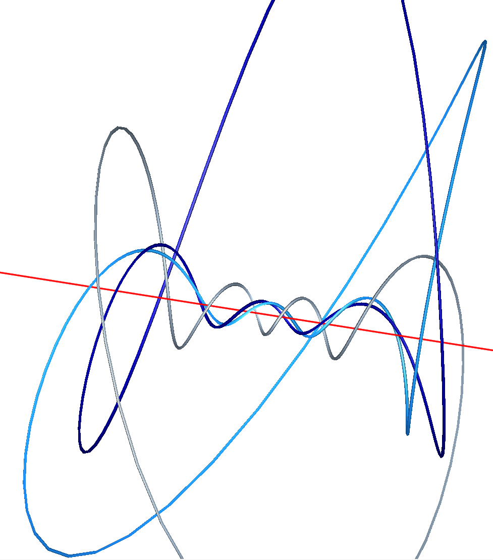
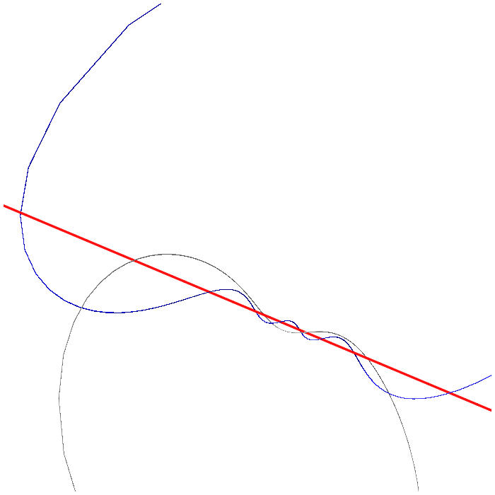
Figure 9: Illustration of $\Delta_{1}$ (Gray) and $\Delta_{2}$ (Blue and Darkblue), linking toric divisor (Red) of $\{z=0\}$ (left) and $\{w=0\}$ (right).

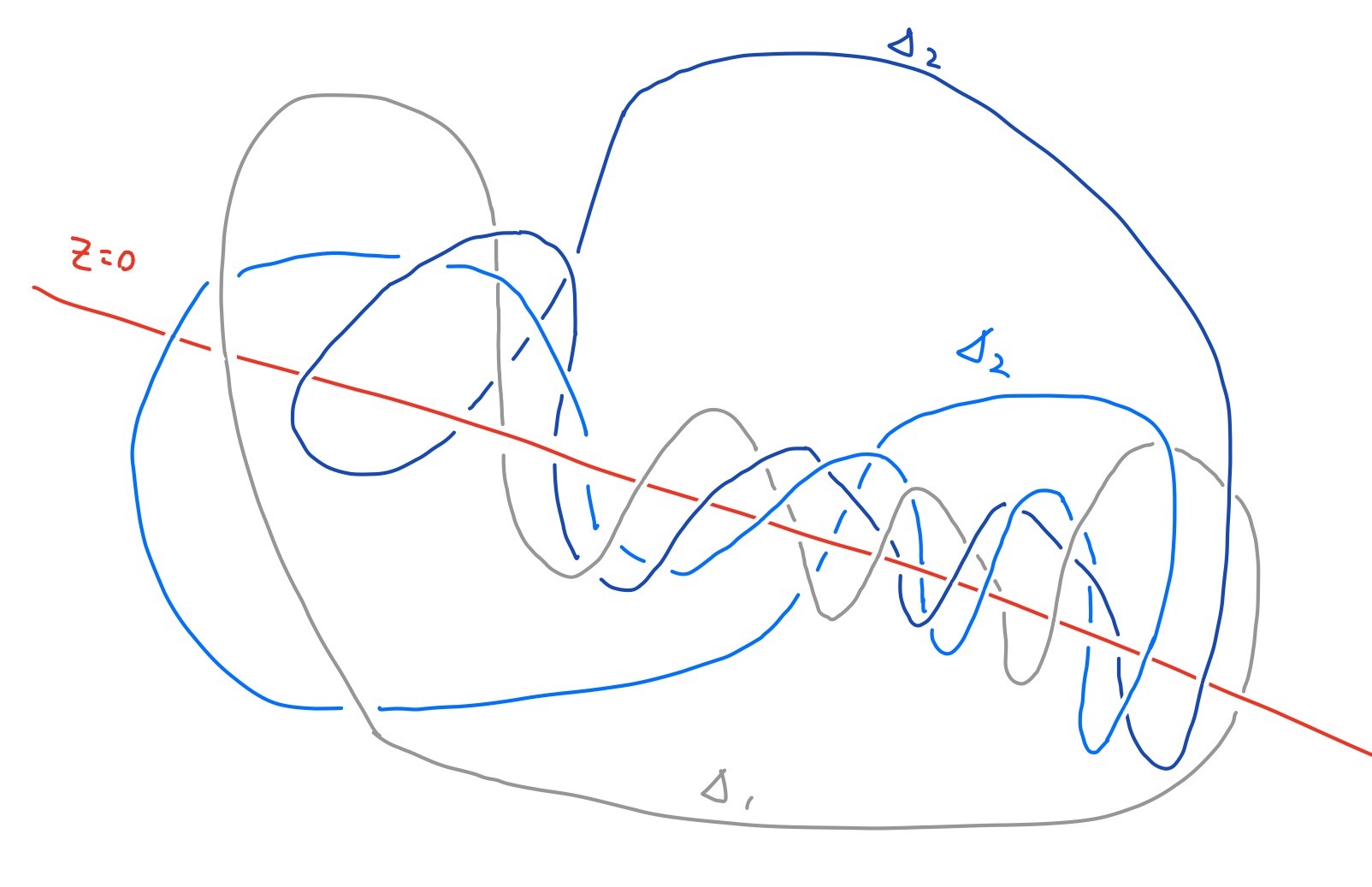
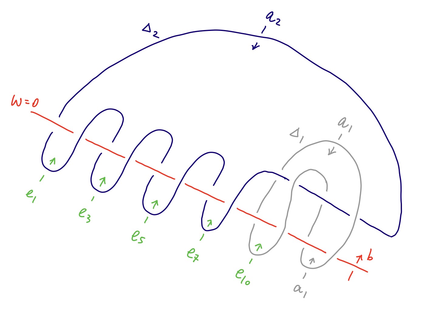
Figure 10: Projection of links around $\{z=0\}$ (left) and $\{w=0\}$ (right)

On the other hand, the link around the $Y$ boundary is a nested toric link that can be analyzed in a similar manner as in the abelian case. The generatos of the fundamental group are given in fig. 10 and their relations can be straightforwardly obtained:

$$(a_{2}b)^{2}(a_{2}ba_{1})^{2}(b^{-1}a_{2}b)=(b^{-1}a_{2}b)(a_{2}b)^{2}(a_{2}ba_{1})^{2}.$$ (5.58)

The loop around the $Y$ boundary (with base point at the $X_{A}$ phase) is homotopically equivalent to $\{w=0\}\cap S^{3}$, hence expressing it in terms of fundamental group generators is straightforward:

$$e_{1}e_{3}e_{5}e_{7}e_{10}a_{1}=b^{-3}(a_{2}b)^{3}a_{1}a_{2}ba_{1}b^{-1}.$$ (5.59)

We then propose the following association of functors to generators:

$$b=T_{(w)},\quad a_{1}=T_{S_{X}},\quad a_{2}=T_{\mathcal{O}_{X}}.$$ (5.60)

It is direct to check (5.58) and (5.59) by assigning the corresponding matrices to the functors (5.60). At the level of functors, we propse then the following relation:

$$T_{Y}=T_{(w)}^{-3}(T_{\mathcal{O}_{X}}T_{(w)})^{3}T_{S_{X}}T_{\mathcal{O}_{X}}T_{(w)}T_{S_{X}}T_{(w)}^{-1}.$$ (5.61)

6 Future directions

In this section we list some challenges and possible future directions to explore.

• Even though we can find the monodromies around discriminat components with relative ease in linear PAX models, we do not have a systematic way to assign functors to each discriminant component, particularly in the nonabelian case, where the techniques of [53] no longer applies. The examples analyzed here and in [59], as well as several unpublished results, seems to suggest that these monodromies remain relatively simple in the nonabelian models, namely they still have the form of a spherical functor $T_{E}$ where the object $E$ is torsion sheaf or locally free sheaf associated with that component of the discriminat. It should be then possible to find some correpondence between GLSM data and number of discriminant components similar to the one that exist in the abelian models [53].

• In our analysis, all the links coming from discriminants in PAX models are found to be of the type of ’nested torus links’, whose fundamental groups were systematically studied in [69]. It would be interesting to further explore how these fundamental group relations impose conditions on the autoequivalences of linear PAX models. In addition, a valid question is how general the phenomenon of these discriminants being nested torus links is.

• A completely new direction would be to study the interaction between the $T_{Y}$, $T_{X}$ functors and their decomposition in the context of Seiberg-like dualities [19]. For instance, the monodromy matrices are expected to remain invariant under duality, but their interpretation can change as the base point can be mapped to a phase whose IR dynamics have a different description.

• In the two-parameter models analyzed here, our derivation of the window categories suggests that we can consider an effective one -parameter model, close to the phase boundaries but keeping $|\zeta_{0}|$ or $|\zeta_{1}|$ large but finite. Then the corresponding FI-theta parameter that is frozen to a large value should act as an effective coupling, spliting the Coulomb branch singularities of the corresponding one-parameter model. This can provide a systematic and unambigous way to determine the assignement between the generators of the fundamental group of the link and functors.

• The assignment of $T_{\mathcal{O}_{X}}$ to the monodromy around a conifold point as a well established mirror interpretation as Dehn twists around a lagrangian spheres [64]. It would be interesting to study the mirror of the functor $T_{S_{X}}$ we found, for instance, in the GN example. Similar functors are also found in [59].

• More complicated examples of determinantal varieties are presented in [6] and their link groups are much more complex. These models can give relations between functors that are mathematically novel.

References

- [1] E. Witten, “Phases of N=2 theories in two-dimensions,” AMS/IP Stud. Adv. Math. 1 (1996) 143–211, hep-th/9301042.
- [2] M. Herbst, K. Hori, and D. Page, “B-type d-branes in toric calabi–yau varieties,” in Homological Mirror Symmetry: New Developments and Perspectives, pp. 1–18. Springer, 2008.
- [3] D. Halpern-Leistner, “The derived category of a git quotient,” Journal of the American Mathematical Society 28 (2015), no. 3, 871–912.
- [4] M. Ballard, D. Favero, and L. Katzarkov, “Variation of geometric invariant theory quotients and derived categories,” Journal für die reine und angewandte Mathematik 2019 (2019), no. 746, 235–303.
- [5] K. Hori and M. Romo, “Exact Results In Two-Dimensional (2,2) Supersymmetric Gauge Theories With Boundary,” 1308.2438.
- [6] H. Jockers, V. Kumar, J. M. Lapan, D. R. Morrison, and M. Romo, “Nonabelian 2D Gauge Theories for Determinantal Calabi-Yau Varieties,” JHEP 11 (2012) 166, 1205.3192.
- [7] M. Herbst, K. Hori, and D. Page, “Phases Of N=2 Theories In 1+1 Dimensions With Boundary,” 0803.2045.
- [8] E. Segal, “Equivalences between GIT quotients of Landau-Ginzburg B-models,” Commun. Math. Phys. 304 (2011) 411–432, 0910.5534.
- [9] J. Clingempeel, B. Le Floch, and M. Romo, “B-brane transport in anomalous (2,2) models and localization,” 1811.12385.
- [10] P. S. Aspinwall, “Some navigation rules for D-brane monodromy,” J. Math. Phys. 42 (2001) 5534–5552, hep-th/0102198.
- [11] K. Hori and M. Romo, “Notes on the hemisphere,” in Primitive Forms and Related Subjects—Kavli IPMU 2014, K. Hori, C. Li, S. Li, and K. Saito, eds., vol. 83 of Advanced Studies in Pure Mathematics, pp. 127–220, Mathematical Society of Japan. Tokyo, 2019.
- [12] C. Schoen, “On the geometry of a special determinantal hypersurface associated to the mumford-horrocks vector bundle.,”.
- [13] M. Gross and S. Popescu, “Calabi–yau threefolds and moduli of abelian surfaces i,” Compositio Mathematica 127 (2001), no. 2, 169–228.
- [14] T. H. Gulliksen and O. Negård, “Un complexe resolvant pour certain idéaux détérminentiels.,” Preprint series: Pure mathematics http://urn. nb. no/URN: NBN: no-8076 (1971).
- [15] J. Harris, “Algebraic geometry: a first course,”.
- [16] D. R. Morrison and M. R. Plesser, “Summing the instantons: Quantum cohomology and mirror symmetry in toric varieties,” Nucl. Phys. B 440 (1995) 279–354, hep-th/9412236.
- [17] K. Hori and D. Tong, “Aspects of Non-Abelian Gauge Dynamics in Two-Dimensional N=(2,2) Theories,” JHEP 05 (2007) 079, hep-th/0609032.
- [18] H. Jockers, V. Kumar, J. M. Lapan, D. R. Morrison, and M. Romo, “Two-Sphere Partition Functions and Gromov-Witten Invariants,” Commun. Math. Phys. 325 (2014) 1139–1170, 1208.6244.
- [19] K. Hori, “Duality In Two-Dimensional (2,2) Supersymmetric Non-Abelian Gauge Theories,” JHEP 10 (2013) 121, 1104.2853.
- [20] C. Schoen, “On the geometry of a special determinantal hypersurface associated to the mumford-horrocks vector bundle.,”.
- [21] M. Gross and S. Popescu, “Calabi–yau threefolds and moduli of abelian surfaces i,” Compositio Mathematica 127 (2001), no. 2, 169–228.
- [22] S. Hosono and H. Takagi, “Mirror symmetry and projective geometry of Reye congruences I,” J. Alg. Geom. 23 (2014), no. 2, 279–312, 1101.2746.
- [23] M. Kapustka and G. Kapustka, “A cascade of determinantal calabi–yau threefolds,” Mathematische Nachrichten 283 (2010), no. 12, 1795–1809.
- [24] M.-A. Bertin, “Examples of calabi–yau 3-folds of p7 with rho=1,” Canadian Journal of Mathematics 61 (2009), no. 5, 1050–1072.
- [25] F. Benini and S. Cremonesi, “Partition Functions of Gauge Theories on S2 and Vortices,” Commun. Math. Phys. 334 (2015), no. 3, 1483–1527, 1206.2356.
- [26] N. Doroud, J. Gomis, B. Le Floch, and S. Lee, “Exact Results in D=2 Supersymmetric Gauge Theories,” JHEP 05 (2013) 093, 1206.2606.
- [27] D. Honda and T. Okuda, “Exact results for boundaries and domain walls in 2d supersymmetric theories,” JHEP 09 (2015) 140, 1308.2217.
- [28] S. Sugishita and S. Terashima, “Exact Results in Supersymmetric Field Theories on Manifolds with Boundaries,” JHEP 11 (2013) 021, 1308.1973.
- [29] S. Cecotti and C. Vafa, “Topological antitopological fusion,” Nucl. Phys. B 367 (1991) 359–461.
- [30] K. Hori, A. Iqbal, and C. Vafa, “D-branes and mirror symmetry,” hep-th/0005247.
- [31] H. Ooguri, Y. Oz, and Z. Yin, “D-branes on Calabi-Yau spaces and their mirrors,” Nucl. Phys. B 477 (1996) 407–430, hep-th/9606112.
- [32] Y.-K. E. Cheung and Z. Yin, “Anomalies, branes, and currents,” Nucl. Phys. B 517 (1998) 69–91, hep-th/9710206.
- [33] M. B. Green, J. A. Harvey, and G. W. Moore, “I-brane inflow and anomalous couplings on d-branes,” Class. Quant. Grav. 14 (1997) 47–52, hep-th/9605033.
- [34] R. Minasian and G. W. Moore, “K theory and Ramond-Ramond charge,” JHEP 11 (1997) 002, hep-th/9710230.
- [35] J. Halverson, H. Jockers, J. M. Lapan, and D. R. Morrison, “Perturbative Corrections to Kaehler Moduli Spaces,” Commun. Math. Phys. 333 (2015), no. 3, 1563–1584, 1308.2157.
- [36] A. Libgober, “Chern classes and the periods of mirrors,” Mathematical Research Letters 6 (1999), no. 2, 141–149.
- [37] S. Hosono, “Local mirror symmetry and type IIA monodromy of Calabi-Yau manifolds,” Adv. Theor. Math. Phys. 4 (2000) 335–376, hep-th/0007071.
- [38] H. Iritani, “An integral structure in quantum cohomology and mirror symmetry for toric orbifolds,” Advances in Mathematics 222 (2009), no. 3, 1016–1079.
- [39] L. Katzarkov, M. Kontsevich, and T. Pantev, “Hodge theoretic aspects of mirror symmetry,” in Proceedings of Symposia in Pure Mathematics, vol. 78, pp. 87–174, American Mathematical Society. 2008.
- [40] E. Witten, “D-branes and K-theory,” JHEP 12 (1998) 019, hep-th/9810188.
- [41] M. Passare, A. Tsikh, and O. Zhdanov, “A multidimensional jordan residue lemma with an application to mellin-barnes integrals,” Contributions to Complex Analysis and Analytic Geometry/Analyse Complexe et Géométrie Analytique: Dedicated to Pierre Dolbeault/Mélanges en l’honneur de Pierre Dolbeault (1994) 233–241.
- [42] O. Zhdanov and A. Tsikh, “Computation of multiple mellin-barnes integrals by means of multidimensional residues,” in Dokl. Akad. Nauk, vol. 358, pp. 154–156. 1998.
- [43] J. Knapp, M. Romo, and E. Scheidegger, “D-Brane Central Charge and Landau–Ginzburg Orbifolds,” Commun. Math. Phys. 384 (2021), no. 1, 609–697, 2003.00182.
- [44] S. Hosono, “Central charges, symplectic forms, and hypergeometric series in local mirror symmetry,” hep-th/0404043.
- [45] S. Hosono, A. Klemm, S. Theisen, and S.-T. Yau, “Mirror symmetry, mirror map and applications to Calabi-Yau hypersurfaces,” Commun. Math. Phys. 167 (1995) 301–350, hep-th/9308122.
- [46] S. Hosono, A. Klemm, S. Theisen, and S.-T. Yau, “Mirror symmetry, mirror map and applications to complete intersection Calabi-Yau spaces,” Nucl. Phys. B 433 (1995) 501–554, hep-th/9406055.
- [47] D. A. Cox and S. Katz, “Mirror symmetry and algebraic geometry, volume 68 of mathematical surveys and monographs,” American Mathematical Society, Providence, RI 21 (1999) 115.
- [48] S. Martin, “Symplectic quotients by a nonabelian group and by its maximal torus,” arXiv preprint math/0001002 (2000).
- [49] J. Guo, M. Romo, and L. Smith to appear.
- [50] W. Donovan and E. Segal, “Window shifts, flop equivalences and grassmannian twists,” Compositio Mathematica 150 (2014), no. 6, 942–978.
- [51] W. Donovan, “Grassmannian twists on the derived category via spherical functors,” Proceedings of the London Mathematical Society 107 (2013), no. 5, 1053–1090.
- [52] M. M. Kapranov, “On the derived categories of coherent sheaves on some homogeneous spaces,” Inventiones mathematicae 92 (1988), no. 3, 479–508.
- [53] I. M. Gelfand, M. M. Kapranov, and A. V. Zelevinsky, “Discriminants, resultants, and multidimensional determinants,”.
- [54] V. V. Batyrev, “Dual polyhedra and mirror symmetry for calabi-yau hypersurfaces in toric varieties,” J. Alg. Geom. 3 (1994) 493–535.
- [55] V. V. Batyrev and L. A. Borisov, “On Calabi-Yau complete intersections in toric varieties,” alg-geom/9412017.
- [56] D. Erkinger and J. Knapp, “Hemisphere Partition Function and Monodromy,” JHEP 05 (2017) 150, 1704.00901.
- [57] R. Eager, K. Hori, J. Knapp, and M. Romo, “Beijing lectures on the grade restriction rule,” Chinese Annals of Mathematics, Series B 38 (2017) 901–912.
- [58] J. Guo, B. Lin, and H. Zou, “A GLSM realization of derived equivalence in models,” 2312.05740.
- [59] R. Eager, K. Hori, J. Knapp, and M. Romo to appear.
- [60] R. Rouquier, “Categorification of sl (2) and braid groups,” Contemph Math 406 (2006).
- [61] R. Anno, “Spherical functors,” 0711.4409.
- [62] R. P. Horja, “Derived category automorphisms from mirror symmetry,” math/0103231.
- [63] D. Huybrechts, Fourier-Mukai transforms in algebraic geometry. Clarendon Press, 2006.
- [64] P. Seidel and R. P. Thomas, “Braid group actions on derived categories of coherent sheaves,” math/0001043.
- [65] P. Candelas, X. De La Ossa, A. Font, S. H. Katz, and D. R. Morrison, “Mirror symmetry for two parameter models. 1.,” Nucl. Phys. B 416 (1994) 481–538, hep-th/9308083.
- [66] P. Candelas, A. Font, S. H. Katz, and D. R. Morrison, “Mirror symmetry for two parameter models. 2.,” Nucl. Phys. B 429 (1994) 626–674, hep-th/9403187.
- [67] J. Stillwell, “Classical topology and combinatorial group theory,” Graduate Texts in Mathematics (1993).
- [68] J. A. Eagon and D. G. Northcott, “Ideals defined by matrices and a certain complex associated with them,” Proceedings of the Royal Society of London. Series A. Mathematical and Physical Sciences 269 (1962), no. 1337, 188–204.
- [69] P. C. Argyres and D. P. Kulkarni, “Fundamental groups for torus link complements,” 1904.10005.