Decoupling Learning and Decision-Making: Breaking the $\mathcal{O}(\sqrt{T})$ Barrier in Online Resource Allocation with First-Order Methods

Abstract

Online linear programming plays an important role in both revenue management and resource allocation, and recent research has focused on developing efficient first-order online learning algorithms. Despite the empirical success of first-order methods, they typically achieve a regret no better than $\mathcal{O}(\sqrt{T})$, which is suboptimal compared to the $\mathcal{O}(\log T)$ bound guaranteed by the state-of-the-art linear programming (LP)-based online algorithms. This paper establishes several important facts about online linear programming, which unveils the challenge for first-order-method-based online algorithms to achieve beyond $\mathcal{O}(\sqrt{T})$ regret. To address the challenge, we introduce a new algorithmic framework that decouples learning from decision-making. More importantly, for the first time, we show that first-order methods can attain regret $\mathcal{O}(T^{1/3})$ with this new framework. Lastly, we conduct numerical experiments to validate our theoretical findings.

1 Introduction

This paper presents a new algorithmic framework to solve the online linear programming (OLP) problem. In this context, a decision-maker receives a sequence of resource requests with bidding prices, and makes irrevocable allocation decisions for these requests sequentially. The goal of OLP is to maximize the accumulated reward subject to a set of inventory constraints. This problem plays an important role in a wide range of applications, such as revenue management [24], resource allocation [13], cloud computing [11], and online advertising [4].

Most state-of-the-art algorithms for OLP are dual linear programming (LP)-based [1, 14, 12, 16, 18]. More specifically, they require solving a sequence of LPs to make online decisions. These LP-based algorithms can attain theoretical lower bounds for their regret as summarized in Table 1, where regret is defined by the gap between the accumulated reward collected by the decision-maker and the reward achieved by the optimal hindsight allocation policy. However, the high computational cost of these LP-based methods prevents them from being applied in many time-sensitive or large-scale problems in practice, such as the online advertising problem [4], where decisions have to be made instantaneously. This challenge motivates a line of recent research using first-order methods to address the online linear programming problem [15, 9, 4, 5], which are more scalable and computationally efficient than LP-based approaches.

Despite the advantage in computational efficiency, first-order methods are still not comparable to LP-based methods in regret in many settings. Existing first-order-method-based OLP algorithms only achieve $\mathcal{O}(\sqrt{T})$ regret bound. The only exception is when the support of resource requests and bidding prices are finite [23]. Under the continuous support setting, it remains an open question:

Can first-order methods go beyond $\mathcal{O}(\sqrt{T})$ regret?

Contributions.

This paper takes a first step towards answering this question with the following contributions:

• We characterize a dilemma empirically and theoretically in applying first-order methods to OLP. The dilemma interprets the difficulty in achieving regret and constraint violation better than $\mathcal{O}(\sqrt{T})$ with first-order algorithms, and also depicts the discrepancy between online decision-making and learning.

• To address the dilemma, we introduce a new online decision-making framework. The idea is to decouple the learning and decision-making procedures with two separate first-order algorithms and achieve better decision-making by efficiently combining them.

• With the help of this new framework, for the first time, we show that first-order-method-based OLP algorithms achieve $\mathcal{O}(T^{1/3})$ regret and constraint violation, which is by far the best result for first-order-based methods under the continuous support setting.

Table 1: Results of regret bounds of the current results. $\log\log$ factors are ignored.

Paper	Setting	Algorithm	Regret	Reaching lower bound
[16]	Continuous support	LP-based	$\mathcal{O}(\log T)$	Yes
[6]	Continuous support	LP-based	$\mathcal{O}(\log T)$	Yes
[12]	Finite support	LP-based	$\mathcal{O}(\log T)$	Yes
[18]	Continuous support	LP-based	$\mathcal{O}(\log T)$	Unknown
[7]	Finite support	LP-based	$\mathcal{O}(1)$	Yes
[15]	Continuous & Finite	First-order Subgradient	$\mathcal{O}(\sqrt{T})$	Yes
[4]	Continuous & Finite	First-order Mirror Descent	$\mathcal{O}(\sqrt{T})$	Yes
[17]	Continuous & Finite	First-order Mirror Descent	$\mathcal{O}(\sqrt{T})$	Yes
[9]	Continuous & Finite	First-order Proximal Point	$\mathcal{O}(\sqrt{T})$	Yes
[5]	Continuous & Finite	First-order and Momentum	$\mathcal{O}(\sqrt{T})$	Yes
[23]	Finite support	First-order Subgradient	$\mathcal{O}(T^{3/8})$	No
This paper	Continuous support	First-order Subgradient	${\color[rgb]{1,0,0}\mathcal{O}(T^{1/3})}$	No

Related Literature.

There is a vast literature on OLP [19, 21, 20, 2], and we review some recent developments that reach beyond $\mathcal{O}(\sqrt{T})$ regret in the stochastic input setting. These algorithms mostly follow the same principle of making decisions based on the learned information: Learning and decision-making are closely coupled with each other. We refer the interested readers to [3] for a more detailed review on OLP and relevant problems.

LP-based Online LP.

Most of the LP-based OLP algorithms are dual-based [1], with only a few exceptions [14]. Under assumptions of either non-degeneracy or finite support on resource requests and/or rewards, $\mathcal{O}(\log T)$ regret bounds have been achieved under different settings. We summarize the results in Table 1. More specifically, [16] establish the dual convergence of finite-horizon LP solution to the optimal dual solution to the underlying stochastic program. In the continuous support setting, the $\mathcal{O}(\log T\log\log T)$ regret is achieved. [6] considers multi-secretary problem and establishes $\mathcal{O}(\log T)$ regret result. [18] consider the setting where a regularization term is imposed on the resource and also established $\mathcal{O}(\log T)$ result. [12] establish $\mathcal{O}(\log T)$ regret, which assumes that customers’ requests are from distribution of finite support. [7] consider the case where customer distribution has finite support, and constant regret can be achieved in this case.

First-order OLP.

Early explorations of first-order-method-based OLP algorithms start from [15] and [4, 17], where $\mathcal{O}(\sqrt{T})$ regret is established using mirror descent and subgradient methods. [9] show that proximal point update also achieves $\mathcal{O}(\sqrt{T})$ regret. Recently, [5] analyze a momentum variant of mirror descent and get $\mathcal{O}(\sqrt{T})$ regret. Under finite support assumption, [23] design a three-stage algorithm that achieves $\mathcal{O}(T^{3/8})$ regret. To our knowledge, this is the only instance of first-order-method-based OLP algorithm that goes beyond $\mathcal{O}(\sqrt{T})$.

Structure of the Paper.

This paper is organized as follows.Section 2 introduces the problem setup and assumptions; In Section 3, we unveil a dilemma between decision-making and learning; In Section 4, we present our framework that decouples learning from decision-making, and show that our framework achieves better regret than $\mathcal{O}(\sqrt{T})$; We conduct numerical experiments in Section 5 to verify our theoretical findings.

2 Problem Setup

Notations. Throughout the paper, we use $\|\cdot\|$ to denote Euclidean norm and $\langle\cdot,\cdot\rangle$ to denote Euclidean inner product. Bold letters notations $\mathbf{A}$ and $\mathbf{a}$ denote matrices and vectors, respectively. Given a convex function, its subdifferential is denoted by $\partial f(\mathbf{x})$ and $f^{\prime}(\mathbf{x})\in\partial f(\mathbf{x})$ is called a subgradient. $[\cdot]_{+}=\max\{\cdot,0\}$ denotes element-wise positive part function and $\mathbb{I}\{\cdot\}$ denotes the 0-1 indicator function. Given total iteration count $T$, we use $\mathcal{O}(1/\sqrt{T}),\mathcal{O}(1/t)$ to denote stochastic gradient-based methods that use fixed stepsize and adaptive stepsizes proportional to $1/t$ respectively.

2.1 Online LP and Duality

Consider online resource allocation over horizon $T\geq 1$: Given initial inventory of $m\geq 1$ resources represented by $\mathbf{b}\in\mathbb{R}^{m}$, at time $t$, an order $(c_{t},\mathbf{a}_{t})\in\mathbb{R}\times\mathbb{R}^{m}$ arrives and requests resource $\mathbf{a}_{t}$ at bidding price $c_{t}$. Decision $x^{t}\in[0,1]$ is made to either accept or reject the order. Define $\mathbf{c}\coloneqq(c_{1},\ldots,c_{T})^{\top}\in\mathbb{R}^{T}$ and $\mathbf{A}\coloneqq(\mathbf{a}_{1},\ldots,\mathbf{a}_{T})\in\mathbb{R}^{m\times T}$, and we write the problem as “offline” LP:

$$\max_{\mathbf{x}} \leavevmode\nobreak\ \leavevmode\nobreak\ \leavevmode\nobreak\ \leavevmode\nobreak\ \leavevmode\nobreak\ \langle\mathbf{c},\mathbf{x}\rangle$$ (PLP)

subject to $$\leavevmode\nobreak\ \quad\mathbf{A}\mathbf{x}\leq\mathbf{b}$$

$$\quad\textbf{0}\leq\mathbf{x}\leq\textbf{1}$$

where 0 and 1 denote vectors of all zeros and ones, respectively. The dual problem of (PLP) is given by

$$\min_{\mathbf{y},\mathbf{s}}\leavevmode\nobreak\ \leavevmode\nobreak\ \langle\mathbf{b},\mathbf{y}\rangle+\langle\textbf{1},\mathbf{s}\rangle$$ (DLP)

$$\text{ subject to }\leavevmode\nobreak\ \leavevmode\nobreak\ \mathbf{A}^{\top}\mathbf{y}+\mathbf{s}\geq\mathbf{c}$$

$$(\mathbf{y},\mathbf{s})\geq\textbf{0}$$

According to [15], (DLP) can be written as

$$\min_{\mathbf{y}\geq\textbf{0}}\quad\textstyle f_{T}(\mathbf{y})\coloneqq\frac{1}{T}\sum_{t=1}^{T}\langle\mathbf{d},\mathbf{y}\rangle+[c_{t}-\langle\mathbf{a}_{t},\mathbf{y}\rangle]_{+},$$ (1)

where $\mathbf{d}=\mathbf{b}/T$ is the average resource and $f_{T}(\mathbf{y})$ can be seen as the sample approximation of the function

$$f(\mathbf{y})\coloneqq\mathbb{E}[f_{T}(\mathbf{y})]=\langle\mathbf{d},\mathbf{y}\rangle+\mathbb{E}_{(c,\mathbf{a})}[[c-\langle\mathbf{a},\mathbf{y}\rangle]_{+}],$$ (2)

if coefficient pairs $(c_{t},\mathbf{a}_{t})$ are drawn from some fixed distribution. Next, we respectively define

$$\mathbf{y}_{T}^{\star}\in \arg\min_{\mathbf{y}\geq\textbf{0}}\leavevmode\nobreak\ f_{T}(\mathbf{y})\quad\text{and}\quad\mathbf{y}^{\star}\in\arg\min_{\mathbf{y}\geq\textbf{0}}\leavevmode\nobreak\ f(\mathbf{y})$$

and optimality conditions build the following connection between the primal-dual optimal solution pair,

$$x_{t}^{\star}\in\left\{\begin{array}[]{ll}\{0\},&c_{t}<\langle\mathbf{a}_{t},\mathbf{y}^{\star}_{T}\rangle,\\ {}[0,1],&c_{t}=\langle\mathbf{a}_{t},\mathbf{y}^{\star}_{T}\rangle,\\ \{1\},&c_{t}>\langle\mathbf{a}_{t},\mathbf{y}^{\star}_{T}\rangle.\end{array}\right.$$ (6)

This connection motivates dual-based online LP methods.

2.2 Dual-based Online LP Algorithms

The dual-based online LP algorithm works as follows: Given an online learning algorithm

$$\mathcal{A}^{t}:=\mathcal{A}(\{(c_{1},\mathbf{a}_{1}),\ldots,(c_{t},\mathbf{a}_{t})\}),$$

we maintain and update a dual sequence $\{\mathbf{y}^{t}\}_{t=1}^{T}$ in an online fashion; primal decisions $\{x^{t}\}_{t=1}^{T}$ are made based on $\{\mathbf{y}^{t}\}_{t=1}^{T}$ and (6). Algorithm 1 illustrates the framework.

Algorithm 1 Dual-based online LP algorithm

Input: $\mathbf{y}^{1},(\mathbf{A},\mathbf{b},\mathbf{c}),$ algorithm $\mathcal{A}$

for $t$ = $1$ to $T$  do

      

$$\mathbf{y}^{t+1}=\mathcal{A}^{t}$$ (7)

Make decision $x^{t}$ by (7) and (6)

end for

Typical choices of $\mathcal{A}$ can be summarized as follows:

• LP-based method: Let $x^{t}=\mathbb{I}\{c_{t}\geq\langle\mathbf{a}_{t},\mathbf{y}_{t}\rangle\}$, solve LP with data $\{(c_{j},\mathbf{a}_{j}),j\leq t\}$ and output $\mathbf{y}^{t+1}=\mathbf{y}_{t}^{\star}$.

• (Sub) Gradient-based method: Let $x^{t}=\mathbb{I}\{c_{t}\geq\langle\mathbf{a}_{t},\mathbf{y}_{t}\rangle\}$, compute subgradient and output $\mathbf{y}^{t+1}$ as follows:

  $$\mathbf{g}_{t}={} \mathbf{d}-\mathbf{a}_{t}x^{t}\in\partial_{\mathbf{y}=\mathbf{y}_{t}}[\langle\mathbf{d},\mathbf{y}\rangle+[c_{t}-\langle\mathbf{a}_{t},\mathbf{y}\rangle]_{+}],$$

  $$\mathbf{y}^{t+1}={} \arg\min_{\mathbf{y}\geq\textbf{0}}\leavevmode\nobreak\ \{\langle\mathbf{g}_{t},\mathbf{y}\rangle+\frac{1}{2\alpha}\|\mathbf{y}-\mathbf{y}^{t}\|^{2}\}.$$ (8)

In this paper, we focus on the gradient-based methods. Variants of the subgradient method, including mirror descent [4] and proximal point [9], have also been analyzed in the literature. Compared to LP-based methods, first-order methods have much lower computational costs and memory requirements.

2.3 Performance Metric

Given output of online algorithm $\hat{\mathbf{x}}=(x^{1},\ldots,x^{T})$, we define regret and constraint violation, respectively, to be

$$r(\hat{\mathbf{x}}) \coloneqq\max_{\mathbf{A}\mathbf{x}\leq\mathbf{b},\mathbf{0}\leq\mathbf{x}\leq\mathbf{1}}\leavevmode\nobreak\ \leavevmode\nobreak\ \langle\mathbf{c},\mathbf{x}\rangle-\langle\mathbf{c},\hat{\mathbf{x}}\rangle,$$ (9)

$$v(\hat{\mathbf{x}}) \coloneqq\|[\mathbf{A}\hat{\mathbf{x}}-\mathbf{b}]_{+}\|.$$ (10)

These metrics are standard when measuring performance of online algorithms [9, 15].

2.4 Assumptions and Auxiliary Results

We make the following assumptions throughout the paper.

1. $\{(c_{t},\mathbf{a}_{t})\}_{t=1}^{T}$ are generated i.i.d. from some distribution $\mathcal{P}$.

2. There exist constants $\bar{a},\bar{c}>0$ such that $\|\mathbf{a}\|_{\infty}\leq\bar{a}$ and $|c|\leq\bar{c}$ almost surely.

3. The average resource $\mathbf{d}=\mathbf{b}/T$ satisfies $\underline{d}\cdot\textbf{1}\leq\mathbf{d}\leq\bar{d}\cdot\textbf{1}$, where $0<\underline{d}\leq\bar{d}$.

4. Second moment $\mathbb{E}[\mathbf{a}\mathbf{a}^{\top}]$ is positive definite with minimum eigenvalue $\lambda_{0}$.

5. There exist $\lambda_{1},\lambda_{2}>0$ such that for $(c,\mathbf{a})\sim\mathcal{P}$,

   $$\lambda_{1}|\langle\mathbf{a},\mathbf{y}-\mathbf{y}^{\star}\rangle|\leq|\mathbb{P}\{c\geq\langle\mathbf{a},\mathbf{y}\rangle|\mathbf{a}\}-\mathbb{P}\{c\geq\langle\mathbf{a},\mathbf{y}^{\star}\rangle|\mathbf{a}\}|\leq\lambda_{2}|\langle\mathbf{a},\mathbf{y}-\mathbf{y}^{\star}\rangle|$$

   for all $\mathbf{y}\in\Xi_{1}\coloneqq\{\mathbf{y}:\mathbf{y}\geq\textbf{0},\|\mathbf{y}\|\leq\frac{\bar{c}}{\underline{d}}+1\}$.

6. $\mathbf{y}^{\star}$ satisfies $y_{i}^{\star}=0$ if and only if $d_{i}-\mathbb{E}_{(c,\mathbf{a})}[a_{i}\mathbb{I}\{c>\langle\mathbf{a},\mathbf{y}^{\star}\rangle\}]>0$ for all $i$.

Remark 1.

The aforementioned assumptions are identical to Assumption 2 from [16], except $\Xi_{1}$ is defined with respect to Euclidean norm for convenience of analysis. To the best of our knowledge, [16] require a stronger version of A5 to get $\mathcal{O}(\log T\log\log T)$ regret, and so far, no algorithm can reach regret beyond $\mathcal{O}(\sqrt{T})$ under exactly the above set of assumptions.

With the assumptions above, we immediately have the following auxiliary results from [16].

Lemma 1 (Proposition 2 in [16]).

Assume A1 to A6 and let $\mu=\frac{\lambda_{0}\lambda_{1}}{2}>0$, then

$$f(\mathbf{y})-f(\mathbf{y}^{\star})-\langle f^{\prime}(\mathbf{y}^{\star}),\mathbf{y}-\mathbf{y}^{\star}\rangle\geq{} \frac{\mu}{2}\|\mathbf{y}-\mathbf{y}^{\star}\|^{2}$$ (11)

$$\langle f^{\prime}(\mathbf{y}^{\star}),\mathbf{y}-\mathbf{y}^{\star}\rangle\geq{} 0,$$

for all $\mathbf{y}\in\Xi_{1}$, where $f^{\prime}(\mathbf{y}^{\star})\in\partial f(\mathbf{y}^{\star})=\{\nabla f(\mathbf{y}^{\star})\}$. Moreover, $\mathbf{y}^{\star}\in\Xi_{0}\coloneqq\{\mathbf{y}:\mathbf{y}\geq\mathbf{0},\|\mathbf{y}\|\leq\frac{\bar{c}}{\underline{d}}\}$ is unique.

Remark 2.

Our algorithm essentially requires the growth condition guaranteed in Lemma 11. In other words, we can also adopt the assumptions from other OLP literature that lead to the growth condition [6, 7, 12, 18].

Lemma 1 shows the expected dual objective (2) has a unique optimal solution and exhibits a quadratic growth property, which is also known as semi-strong convexity [26]. Since [16] achieves $\mathcal{O}(\log T\log\log T)$ regret with a slightly stronger version of A5 and Lemma 1, it is natural to expect that first-order algorithms may also achieve regret better than $\mathcal{O}(\sqrt{T})$. However, in the next section, we present a dilemma for first-order algorithms in OLP, which almost prevents them from achieving better performance.

3 Dilemma between Learning and Decision-making

In this section, we discuss a dilemma between learning and decision-making for first-order algorithms in OLP. That is, although achieving a better estimation of $\mathbf{y}^{\star}$ benefits decision-making, the small stepsize in first-order algorithms with fast convergence rate prevent them from good decision-making.

3.1 Benefit in Learning Better

We start from discussing the benefit of learning a better dual solution for the dual-based online algorithm (Algorithm 1) by the following proposition.

Proposition 1.

Under A1 to A6, given an estimate $\mathbf{y}^{1}$ of $\mathbf{y}^{\star}$ such that

$$\|\mathbf{y}^{1}-\mathbf{y}^{\star}\|=\mathcal{O}(1/T^{\theta}),$$

for some $\theta\geq 0$, then Algorithm 1 with the subgradient update (8) and stepsize $\mathcal{O}(T^{-\frac{2\theta^{\prime}+1}{2\theta^{\prime}+2}})$ achieves ${\mathcal{O}}(T^{\frac{1}{2\theta^{\prime}+2}})$ regret and constraint violation simultaneously, where $\theta^{\prime}=\min\{\theta,1/2\}$.

Proposition 1 shows a better estimate of $\mathbf{y}^{\star}$ benefits the performance of OLP algorithms. In particular, when $\mathbf{y}^{1}=\mathbf{y}^{\star}$, $\mathcal{O}(T^{1/3})$ regret and constraint violation are achieved at the same time.

Proposition 1 also reveals the significance of the knowledge about the distribution $\mathcal{P}$. Specifically, [16] show that even if the distribution $\mathcal{P}$ is known, and that $\mathbf{y}^{\star}$ can be computed prior to the decision-making process, Algorithm 1 with $\mathbf{y}^{t}=\mathbf{y}^{\star}$ for all $t$ only achieves $\mathcal{O}(\sqrt{T})$ regret under A1 to A6. Results from [16] seem to suggest that knowing $\mathcal{P}$ does not yield an improvement beyond $\mathcal{O}(\sqrt{T})$. However, Proposition 1 points out that this knowledge at least helps obtain $\mathcal{O}(T^{1/3})$ regret, thereby opening up the possibility of achieving even better regret with knowledge of the distribution $\mathcal{P}$.

To understand this discrepancy between [16] and Proposition 1, we remark that Proposition 1 complements rather than conflicts with the results in [16]. In particular, as mentioned in [16], $\mathbf{y}^{\star}$, the dual optimal solution for the expected problem (2), can be different from $\mathbf{y}^{\star}_{T}$, the dual optimal solution of the realized problem (1) due to randomness. The fluctuations can result in a $\mathcal{O}(\sqrt{T})$ regret and constraint violation. Compared to making decisions based on a fixed dual solution $\mathbf{y}^{\star}$, Proposition 1 suggests that combining $\mathbf{y}^{\star}$ with SGD leads to a better regret. In other words, dual solution has to be adjusted, to adapt to noise from the environment.

Although $\mathbf{y}^{\star}$ brings benefits for OLP, we do not have $\mathbf{y}^{\star}$ in practice. As a result, $\mathbf{y}^{\star}$ also needs to be learned along the horizon $T$. However, $\theta=0$ in Proposition 1 still yields $\mathcal{O}(\sqrt{T})$ regret: the proposed algorithm in Proposition 1 cannot achieve better regret and constraint violation than $\mathcal{O}(\sqrt{T})$ by itself. This issue also exists in the current literature about first-order algorithms for OLP. Specifically, the existing first-order algorithms used in OLP [15, 4, 5] are sub-optimal in learning $\mathbf{y}^{\star}$. They share the same convergence rate as the first algorithm listed in Table 2, but they are worse than other algorithms in Table 2 which are designed to exploit the quadratic growth property (11). Thus, one natural expectation is that, first-order algorithms performing better in learning contribute to better decision-making. However, this intuition is not correct.

Table 2: First-order methods for problems with quadratic growth property (11). SGD with $\mu$ refers to subgradient method with known growth parameter $\mu$. Stepsizes of ASSG and SADAGRAD decay to $\mathcal{O}(1/T)$ in the last $\mathcal{O}(T)$ iterations; ASSG and SADAGRAD are parameter-free with respect to $\mu$.

Algorithm	Stepsize	Convergence Rate $\|\mathbf{y}^{k}-\mathbf{y}^{\star}\|$	Parameter Free
SGD [10]	$\mathcal{O}(1/\sqrt{T})$	$\mathcal{O}(1/k^{1/4})$ for all $k=1,\dots,T$	Yes
SGD with known $\mu$ [22]	$\mathcal{O}(1/(\mu t))$	$\mathcal{O}(1/\sqrt{k})$ for all $k=1,\dots,T$	No
Parameter-free ASSG [25]	$\mathcal{O}(1)$ to $\mathcal{O}(1/T)$	$\mathcal{O}(1/\sqrt{T}),k=T$	Yes
Parameter-free SADAGRAD [8]	$\mathcal{O}(1)$ to $\mathcal{O}(1/T)$	$\mathcal{O}(1/\sqrt{T}),k=T$	Yes

3.2 Impossibility in Deciding Better

We now investigate the performance of Algorithm 1 with first-order algorithms that are better in learning $\mathbf{y}^{\star}$, such as SGD with known $\mu$, ASSG, and SADAGRAD in Table 2. Unfortunately, achieving regret better than $\mathcal{O}(\sqrt{T})$ remains impossible even with those good first-order algorithms. Particularly, we illustrate this impossibility by considering the following one-dimensional linear programming problem (12), also known as the online multi-secretary problem:

$$\max_{0\leq x^{t}\leq 1}\leavevmode\nobreak\ \sum\limits_{t=1}^{T}c_{t}x^{t}\leavevmode\nobreak\ \leavevmode\nobreak\ \text{subject to}\quad\sum\limits_{t=1}^{T}x^{t}\leq\frac{T}{2}.$$ (12)

Here, $c_{t}$ is sampled uniformly from $[0,1]$ for all $t=1,\dots,T$. We can compute $\mu=1$, $y^{\star}=1/2$ is the median of the distribution of the objective, and $y_{T}^{\star}$ is the median of the realized samples $\{c_{t}\}_{t=1}^{T}$. As Figure 1 (b) suggests, SGD with known $\mu$ and SADAGRAD indeed learns $y^{\star}$ efficiently. However, their regret and constraint violation bounds still grow at order $\mathcal{O}(\sqrt{T})$ (Figure 1 (a)).

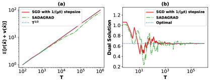
Figure 1: Performance of Algorithm 1 with algorithms of faster convergence rates. (a). performance for Algorithm 1 with algorithms of faster convergence rate: This log-log plot shows that the incurred regrets and constraint violations of Algorithm 1 with 1) SGD and known $\mu$. 2) SADAGRAD have the same growth rate as the function $\sqrt{T}$. (b). convergence and slow updates of the estimated dual solutions.

To interpret this suboptimal performance of these gradient descent methods with fast convergence rate, one key factor is their limited capability in mistake correction. Note that all these algorithms share a similarity that their stepsizes are $\mathcal{O}(1/T)$ in the last $\mathcal{O}(T)$ iterations. This choice of stepsize is required to guarantee fast convergence, but it simultaneously reduces the adaptivity of the dual solution. Consequently, once a mistake is made in estimating the dual solution (i.e., the gap between the estimated dual solution and $\mathbf{y}^{\star}$ is large), these algorithms cannot correct the estimation error for a long time (Figure 1 (b)). This estimation error will lead to suboptimal decisions thereafter, even until the end of the horizon. The following proposition theoretically illustrates this slow-updating issue for SGD with known $\mu$.

Proposition 2.

Denote $y^{t}$ as the estimated dual solution for the online secretary problem (12) at time $t$ by SGD with known $\mu$. If there exists $t_{0}\geq T/10+1$ such that $y^{t_{0}}\geq y^{\star}+\frac{1}{\sqrt{T}}$, then $\mathbb{E}[y^{t}|y^{t_{0}}]\geq y^{\star}+\frac{1}{20\sqrt{T}}$ for all $t\geq t_{0}$.

Proposition 2 tells that once SGD with known $\mu$ estimates the dual optimal solution with an $\mathcal{O}(1/\sqrt{T})$ error for one step, this error cannot be corrected and will be carried for all succeeding steps on expectation. In fact, a similar disability in mistake correction also happens to other algorithms with stepsize $\mathcal{O}(1/T)$ in Table 2, which is shown in Appendix C.4. More importantly, as shown in Proposition 3, this lack of mistake correction ability leads to suboptimal performance in decision-making, ruling out their possibility of achieving regret and constraint violation better than $\mathcal{O}(\sqrt{T})$.

Proposition 3.

Algorithm 1 using SGD with known $\mu$ cannot achieve $\mathcal{O}(T^{\beta})$ regret and constraint violation simultaneously for any $\beta<\frac{1}{2}$.

We have shown so far that the discrepancy between online learning and decision-making: Algorithms efficient in learning fail to achieve regret and constraint violation better than $\mathcal{O}(\sqrt{T})$. Conversely, the preceding part shows the importance of online learning in online decision-making: For some first-order algorithms specialized in decision-making, to achieve regret and constraint violation better than $\mathcal{O}(\sqrt{T})$, a good estimation of the dual optimal solution is required. However, these algorithms cannot learn a good dual solution on their own. These two sides depict the dilemma in first-order-method-based OLP algorithms: first-order algorithms are not good at learning and making decisions simultaneously.

Escaping the Horns of a Dilemma.

The aforementioned dilemma seems discouraging for applying first-order algorithms in online linear programming or online decision-making. However, this dilemma is built on the assumption that one learns a sequence of dual solutions and makes decisions solely based on the same learned sequence. To address this challenge, in the next section, we introduce a two-path approach for online decision-making that maintains decision-making and learning paths independently. This new approach enjoys the strengths of both aspects, which leads to a first-order algorithm achieving $\mathcal{O}(T^{1/3})$ regret and constraint violation without knowledge of $\mathbf{y}^{\star}$.

4 Decoupling Learning and Decision-Making

In this section, we present the framework of our learning algorithm. The dilemma we discussed in the previous section reveals a critical challenge: We may not be able to find a first-order algorithm good at both learning and decision-making. However, the low cost of first-order methods opens up another way: instead of having to choose between learning and decision-making, we take the best of both worlds using two different algorithms simultaneously: a learning algorithm $\mathcal{A}_{L}$ and a decision algorithm $\mathcal{A}_{D}$.

This simple idea yields a highly flexible framework:

1. We can choose $\mathcal{A}_{L}$ and $\mathcal{A}_{D}$ to be good learning and decision algorithms respectively.

2. Information from $\mathcal{A}_{L}$ can be flexibly incorporated into $\mathcal{A}_{D}$. We note that this framework can also be applied to problems beyond online linear programming.

To illustrate the power of this framework, we show how its simple variant breaks the $\mathcal{O}(\sqrt{T})$ barrier of OLP.

4.1 Algorithm Design

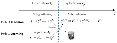
Figure 2: Left: two-path and two-phase decision algorithm. Right: illustration of restart: exploration phase sends $\mathbf{y}^{T_{e}}$ into a neighborhood of $\mathbf{y}^{\star}$, and in the exploitation phase, $\mathbf{y}^{t}$ stays in this neighbor with sufficient stepsize to make adjustments.

We are now ready to introduce our algorithm, a realization of the aforementioned framework. We start by choosing $\mathcal{A}_{D}$ to be subgradient method and $\mathcal{A}_{L}$ to be any of the algorithms from Table 2. $\mathcal{A}_{D}$ and $\mathcal{A}_{L}$ generate two paths of dual sequences $\{\mathbf{y}^{t}\}_{t=1}^{T}$ and $\{\mathbf{y}^{t}_{L}\}_{t=1}^{T}$ respectively. $\mathcal{A}_{D}$ accesses information from $\mathcal{A}_{L}$ with a one-time restart strategy: we divide horizon $T$ into two phases: exploration and exploitation (Figure 2 and Algorithm 2).

Exploration. During exploration phase from $t=1$ to $T_{e}$, $\mathcal{A}_{D}$ and $\mathcal{A}_{L}$ run simultaneously but independently. Subgradient $\mathcal{A}_{D}$ is equipped with stepsize $\alpha_{e}$.

Exploitation. At $t=T_{e}+1$, $\mathcal{A}_{D}$ restarts from $\mathbf{y}^{T_{e}+1}_{L}$ with a different stepsize $\alpha_{p}$. Due to our simple one-time restart strategy, $\mathcal{A}_{L}$ stops after $t\geq T_{e}+1$, $\mathbf{y}^{t}_{L}\equiv\mathbf{y}^{T_{e}+1}_{L},t>T_{e}$.

Algorithm 2 Decoupling learning and decision-making

Input: $\mathbf{y}^{1},(\mathbf{A},\mathbf{b},\mathbf{c}),$ $\mathcal{A_{L}},\mathcal{A_{D}},\alpha_{e},\alpha_{p}$

explore for $t$ = $1$ to $T_{e}$  do

       $\mathbf{y}^{t+1}=\mathcal{A}^{t}_{D}$ with stepsize $\alpha_{e}$ and make decision $x^{t}$ $\mathbf{y}_{L}^{t+1}=\mathcal{A}^{t}_{L}$

end for

restart $\mathcal{A_{D}}$ by $\mathbf{y}_{L}^{T_{e}+1}$ exploit for $t$ = $T_{e}+1$ to $T$  do

       $\mathbf{y}^{t+1}=\mathcal{A}^{t}_{D}$ with stepsize $\alpha_{p}$ and make decision $x^{t}$

end for

Remark 3.

Algorithm 2 is a simple realization of our framework, and the framework can be implemented very flexibly, for example, by using different $\mathcal{A}_{D}$ or with a multi-stage restart strategy.

4.2 Algorithm Analysis

The next two lemmas show the regret and violation using the aforementioned two-path two-phase algorithm.

Lemma 2 (Regret).

Assuming A1 to A6 hold, we have

$$\mathbb{E}[r(\hat{\mathbf{x}})]\leq{} \frac{m(\bar{a}+\bar{d})^{2}\alpha_{e}}{2}T_{e}+\frac{m(\bar{a}+\bar{d})^{2}\alpha_{p}}{2}T_{p}+\frac{\mathsf{R}}{\alpha_{p}}\mathbb{E}[\|\mathbf{y}^{T_{e}+1}-\mathbf{y}^{\star}\|+\|\mathbf{y}^{T+1}-\mathbf{y}^{\star}\|],$$

where $\mathsf{R}\coloneqq\frac{\bar{c}}{\underline{d}}+\big{[}\frac{m(\bar{a}+\bar{d})^{2}}{2\underline{d}}+\sqrt{m}(\bar{a}+\bar{d})\big{]}\cdot\max\{\alpha_{e},\alpha_{p}\}$.

Lemma 3 (Violation).

Assuming A1 to A6 hold, we have

$$\mathbb{E}[v(\hat{\mathbf{x}})]\leq\frac{\mathsf{R}}{\alpha_{e}}+\frac{1}{\alpha_{p}}\mathbb{E}[\|\mathbf{y}^{T_{e}+1}-\mathbf{y}^{\star}\|+\|\mathbf{y}^{T+1}-\mathbf{y}^{\star}\|],$$

where $\mathsf{R}$ is defined in Lemma 2.

Remark 4.

Lemma 2 and 3 suggest that the distance to $\mathbf{y}^{\star}$ indeed plays a role in the bound. However, we also see that: 1). $T_{e}$ cannot be too large, since the best we can do in exploration phase is $\mathcal{O}(\sqrt{T_{e}})$, and we cannot spend too much time in exploration; 2). The distance term is dominated by $\|\mathbf{y}^{T_{e}+1}-\mathbf{y}^{\star}\|$ rather than $\|\mathbf{y}^{T}-\mathbf{y}^{\star}\|$ alone. These two facts suggest that if overly small stepsize is used to reduce $\|\mathbf{y}^{T}-\mathbf{y}^{\star}\|$, the dominating term $\frac{1}{\alpha_{p}}\|\mathbf{y}^{T_{e}+1}-\mathbf{y}^{\star}\|$ will instead blow up, which aligns with our observation from Section 3. In other words, after $T_{e}$ steps of exploration drive $\mathbf{y}^{T_{e}}$ to the proximity of $\mathbf{y}^{\star}$, the most “economical” strategy is to keep impetus and travel around within this neighborhood. Therefore, $\alpha_{p}$ should be determined by the radius of this neighborhood.

After establishing enough intuitions, we now present instances of $(\mathcal{A}_{L},T_{e},\alpha_{e},\alpha_{p})$ in the theorem below.

Theorem 1.

Assuming A1 to A6 hold, then for all $T\geq\frac{36m(\bar{a}+\bar{d})^{2}}{\underline{d}}$, we have:

1. If $T_{e}=0$, there is no exploration. With $\alpha_{p}=T^{-1/2}$,

   $$\mathbb{E}[r(\hat{\mathbf{x}})+v(\hat{\mathbf{x}})]\leq\mathcal{O}(\sqrt{T}).$$

2. If $\mathcal{A}_{L}$ is taken to be SGD with stepsize $\mathcal{O}(1/\sqrt{T_{e}})$, then with $T_{e}=T^{4/5},\alpha_{e}=T^{-2/5},\alpha_{p}=T^{-3/5}$,

   $$\mathbb{E}[r(\hat{\mathbf{x}})+v(\hat{\mathbf{x}})]\leq\mathcal{O}(T^{2/5}).$$

3. If $\mathcal{A}_{L}$ is taken to be SGD with stepsize $\mathcal{O}(1/(\mu t))$, then with $T_{e}=T^{2/3},\alpha_{e}=T^{-1/3},\alpha_{p}=T^{-2/3}$,

   $$\mathbb{E}[r(\hat{\mathbf{x}})+v(\hat{\mathbf{x}})]\leq\mathcal{O}(T^{1/3}).$$

4. If $\mathcal{A}_{L}$ is taken to be either ASSG or SADAGRAD, then with $T_{e}=T^{2/3},\alpha_{e}=T^{-1/3},\alpha_{p}=T^{-2/3}$,

   $$\mathbb{E}[r(\hat{\mathbf{x}})+v(\hat{\mathbf{x}})]\leq\mathcal{O}(T^{1/3}\log T).$$

Based on the learning ability of $\mathcal{A}_{L}$, there exists some choice of $(T_{e},\alpha_{a},\alpha_{p})$ that captures the best trade-off between exploration and exploitation. Using this framework, the $\mathcal{O}(\sqrt{T})$ barrier in online LP is broken.

Discussion on $\mu$.

We make some remarks on the effect of parameter $\mu$. First, as in strongly convex optimization, only an upper bound of $\mu$ is needed for the algorithm to work. Second, even if there is no way to estimate $\mu$, we can use parameter-free algorithms discussed in M3, which will incur a $\log T$ factor but can exhibit much better dependency in constant. Finally, even if for some problems $\mu$ is close to 0 (as we will demonstrate in the experiment), our algorithm is still robust and exhibits $\mathcal{O}(\sqrt{T})$ regret empirically.

5 Numerical Experiments

This section conducts experiments to illustrate the performance and the theoretical results of our framework. In particular, we consider a benchmark algorithm from literature,

• M0: No exploration with $T_{e}=0$ and $\alpha_{p}=T^{-1/2}$.

and two instances from Theorem 1.

• M1: $\mathcal{A}_{L}$ and $\mathcal{A}_{D}$ are both SGD with fixed stepsize $T_{e}^{-1/2}$ in the first $T_{e}=T^{4/5}$ time period.

• M2: $\mathcal{A}_{L}$ is SGD with $\mathcal{O}(1/(\mu t))$ stepsize and $\mathcal{A}_{D}$ is SGD with stepsize $T_{e}^{-1/2}$ in the first $T_{e}=T^{2/3}$ time. We always take $\mu=1$, and do not tune it through the experiments.

Our experiment contains three parts. In the first part, we generate different distributions of $\{(c_{t},\mathbf{a}_{t})\}_{t=1}^{T}$ that satisfy the assumptions specified in Section 2, and assess the above three algorithms’ performance. In the second part, we turn to the distributions that violate at least one of the assumptions and discuss the performance of our algorithm. Finally, we justify the optimality of our stepsize choice in the third experiment.

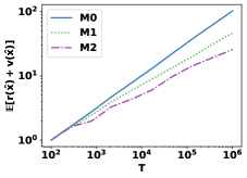
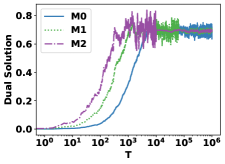
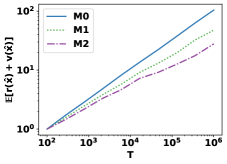
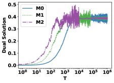
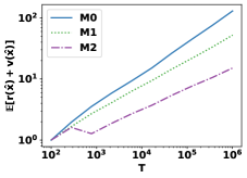
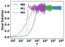
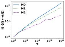
Figure 3: Growth of normalized $r(\hat{\mathbf{x}})+v(\hat{\mathbf{x}})$ and dual convergence of algorithms when the assumptions hold. Each pair of the left figure and the right figure is plotted based on the experiment on the same distribution.

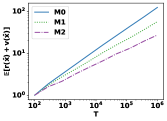
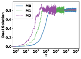
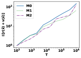
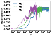
Figure 4: Growth of normalized $r(\hat{\mathbf{x}})+v(\hat{\mathbf{x}})$ of three tested algorithms when the assumptions are violated. The left two: normal distribution; the right two: discrete distribution.

5.1 Performance under Assumptions

In this part, we randomly generate $\{(c_{t},\mathbf{a}_{t})\}_{t=1}^{T}$ from distributions satisfying A1 to A6. Three algorithms’ performance is evaluated in terms of $r(\hat{\mathbf{x}})+v(\hat{\mathbf{x}})$.

We choose $m\in\{1,5\}$ and $T$ evenly spaced over $[10^{2},10^{6}]$ on $\log$-scale. For each value of $T$, each algorithm’s performance is averaged over $100$ random trials under each distribution. For all the distributions, each $d_{i}$ is sampled i.i.d. from uniform distribution $\mathcal{U}[1/3,2/3]$. $\{(c_{t},\mathbf{a}_{t})\}_{t=1}^{T}$ is generated in the following way: 1). For the first distribution [15], we take $m=1$, and sample each $a_{it}$ and $c_{t}$ i.i.d. from $\mathcal{U}[0,2]$; 2). For the second distribution [16], we let $m=1$ and each $a_{it}=1$, and randomly sample each $c_{t}$ i.i.d. from $\mathcal{U}[0,1]$; 3). For the third distribution [16], we randomly generate $a_{it}$ from the truncated standard Cauchy distribution with the location parameter $1$ and the threshold $\pm 10$, and let $c_{t}=\sum_{i=1}^{m}a_{it}-\varepsilon_{t}$ with $\varepsilon_{t}$ from $\mathcal{U}[0,m]$; 4). For the fourth distribution, we let $m=5$, sample $a_{it}$ and $c_{t}$ i.i.d. from the $\mathcal{U}[1,6]$ and $\mathcal{U}[0,3]$, respectively.

For each distribution and algorithm, we normalize the average of $r+v$ by its minimal empirical value and plot its growth behavior with respect to $T$. Then we fix $T=10^{6}$ and plot the convergence of $\{y^{t}\}_{t=1}^{T}$ for the case $m=1$ and the last coordinate of $\mathbf{y}^{t}_{m}$ for the case $m=5$. Figure 3 clearly suggests that M1 and M2 have better order of performance compared to M0, which is consistent with our theory. Meanwhile, the dual solution in M0 converges slower than in M1, M2, and exhibits more oscillation around the optimal dual solution $\mathbf{y}^{\star}$.

5.2 Performance under Violated Assumptions

In the second part, we turn to distributions that violate at least one of the assumptions from A1 to A6. We choose $m,$ $T$ and generate $\{d_{i}\}$ as in the first experiment. We generate $\{(c_{t},\mathbf{a}_{t})\}_{t=1}^{T}$ as follows. 1). For the first distribution [15], we take $m=1$, and each $a_{it}$ is generated from normal distribution $\mathcal{N}(1,1)$. We let each $c_{t}=\sum_{i=1}^{m}a_{it}-\varepsilon_{t}$ with $\varepsilon_{t}$ from $\mathcal{U}[0,m]$. This distribution violates A2. 2). The second distribution has finite support and violates A5. More specifically, we choose $m=1$ and randomly generate $10$ different pairs of $(c_{t},\mathbf{a}_{t})$. Each $c_{t}$ and each element in $\mathbf{a}_{t}$ is sampled from $\mathcal{U}[0,1]$. After obtaining $\{(c_{t},\mathbf{a}_{t})\}_{t=1}^{T}$, at each time period $t$, we sample $(c_{t},\mathbf{a}_{t})$ from these pairs uniformly.

As in the first experiment, Figure 4 plots the growth of normalized $r+v$ and convergence of $\{y^{t}\}_{t=1}^{T}$. M1 and M2 perform better than M0 under the first distribution, with the order still being $\mathcal{O}(T^{1/3})$. Even for the discrete distribution, M1 and M2 still exhibit slightly better performance than M0. This further shows the robustness of our methods.

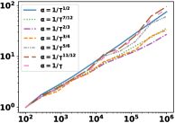
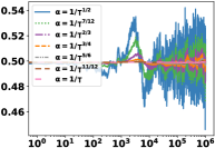
Figure 5: Left: $y$-axis: normalized $r(\hat{\mathbf{x}})+v(\hat{\mathbf{x}})$ under different choices of $\alpha_{p}$. $x$-axis: different $T$. Right: Dual convergence under different $\alpha_{p}$.

5.3 Validation of Stepsize Choice

Our last experiment serves as a validation of our theoretical analysis. Theorem 1 shows that there exists an optimal choice of $\alpha_{p}$ and for M2 the choice is ${T^{-2/3}}$. To verify this, we search $\alpha_{p}=T^{-\beta},\beta\in\{\tfrac{1}{2},\tfrac{7}{12},\tfrac{2}{3},\tfrac{3}{4},\tfrac{5}{6},\tfrac{11}{12},1\}$ and record performance of algorithms under different stepsizes. We also plot the dual convergence behavior for $T=10^{6}$ as in previous subsections. Figure 5 suggests that the best choice of $\alpha_{p}$ exactly appears around $T^{-2/3}$, which verifies our theoretical findings.

6 Conclusion

In this paper, we unveil a dilemma of first-order-method-based online linear programming algorithms. We develop a novel online learning framework that decouples learning and decision-making, which for the first time achieves better than $\mathcal{O}(\sqrt{T})$ regret under continuous distribution assumption. Our new framework and analysis provide new insights for online linear programming, which we believe may be of independent interest and can motivate new algorithms and better theoretical guarantees for online decision-making problems.

Appendix

Structure of the Appendix

The appendix is organized as follows. In Section A, we introduce auxiliary results for the discussion of our framework; Section B presents our two-path two-phase algorithm in a more general framework; Section C, D prove the main results in our paper.

Appendix A Auxiliary Results

In this section, we provide auxiliary results and definitions that will help present our main results. We start by assuming the existence of a dual algorithm with $\theta$-convergence rate.

A.1 $\theta$-Convergence Rate of Dual Learning Algorithms

Proposition 4.

In online LP, a dual learning algorithm $\mathcal{A}_{t}=\mathcal{A}(\{(c_{j},\mathbf{a}_{j}),j\leq t\})$ has $\theta$-convergence rate if at least with probability $1-\frac{1}{T}$, it output $\mathcal{A}_{T}=\mathbf{y}^{T}$ such that

$$\mathbb{E}[\|\mathbf{y}^{T+1}-\mathbf{y}^{\star}\|]\leq\frac{c_{1}+c_{2}\log T}{T^{\theta}},$$

where $c_{1},c_{2}>0$ are constants independent of $T$.

Given a learning algorithm, Proposition 4 can be verified through its convergence results. Here are some examples.

Table 3: Summary of convergence rates

Algorithm	First-order	Knowledge of $\mu$	$\theta$	$c_{2}$
LP-resolving li2022online	No	No	$1/2$	$>0$
God’s perspective	–	–	$\infty$	$=0$
Subgradient with stepsize $1/\sqrt{T}$	Yes	No	$1/4$	$=0$
Subgradient with stepsize $\alpha_{t}=\mathcal{O}(1/(\mu t))$	Yes	Yes	$1/2$	$=0$
Parameter-free ASSG xu2017stochastic	Yes	No	$1/2$	$>0$
Parameter-free SADAGRAD chen2018sadagrad	Yes	No	$1/2$	$=0$

If $\theta=0$, the dual iteration does not converge. On the other hand, by $\theta=\infty$, we mean the algorithm outputs exactly $\mathbf{y}^{\star}$. This happens, for example, if the distribution $\mathcal{P}$ is known. From now we assume the existence of a dual learning algorithm with convergence rate $\theta>0$.

1. There exists a learning algorithm with convergence rate $\theta>0$.

A.2 Verification of Convergence Rates

In this subsection, we verify the choice of $\theta,c_{1},c_{2}$ for the aforementioned algorithms.

A.2.1 LP-resolving

In LP-resolving, we have $\mathbf{y}^{T}=\mathbf{y}_{T}^{\star}$ and we have the following result.

Lemma 4 (li2022online).

Assume that A1 to A6 hold and that $T\geq\max\{m,3\}$. Then there exists some constant $C>0$ such that

$$\mathbb{E}[\|\mathbf{y}^{T+1}-\mathbf{y}^{\star}\|]\leq\frac{C\sqrt{(m\log m+1)\log\log T}}{\sqrt{T}}$$

Lemma 5.

LP-resolving satisfies $\theta=1/2$.

A.2.2 Subgradient

Analysis of subgradient is similar to that in strongly convex case lacoste2012simpler, where, at each iteration

$$\mathbf{y}^{t+1}=\Pi_{\mathbb{R}_{+}^{m}\cap\Xi_{0}}(\mathbf{y}^{t}-\alpha_{t}\mathbf{g}^{t})$$ (13)

for some stepsize $\alpha_{t}$ and $\Pi_{\mathcal{S}}(\cdot)$ denotes orthogonal projection onto set $\mathcal{S}$. Unless specified, we will use $\Pi(\cdot)$ to denote $\Pi_{\mathbb{R}_{+}^{m}\cap\Xi_{0}}(\cdot)$ to simplify notation. The following lemma characterizes behavior of subgradient method.

Lemma 6.

Assume that A1 to A6 hold, then subgradient update (13) satisfies

$$\mathbb{E}_{t}[\|\mathbf{y}^{t+1}-\mathbf{y}^{\star}\|^{2}]\leq(1-\alpha_{t}\mu)\|\mathbf{y}^{t}-\mathbf{y}^{\star}\|^{2}+\alpha^{2}_{t}m(\bar{a}+\bar{d})^{2}$$

for all $t\geq 1$, where $\mathbb{E}_{t}[\cdot]\coloneqq\mathbb{E}[\cdot|\{(c_{j},\mathbf{a}_{j}),j\leq t\}]$ denotes conditional expectation on history.

Plugging in different choices of $\alpha_{t}$, a telescopic sum completes the proof.

Lemma 7 (Subgradient with constant stepsize).

Under the same assumptions as Lemma 6, if $\alpha_{t}\equiv\alpha$, then

$$\mathbb{E}_{t}[\|\mathbf{y}^{T+1}-\mathbf{y}^{\star}\|^{2}]\leq\frac{\Delta^{2}}{\mu\alpha T}+\frac{m(\bar{a}+\bar{d})^{2}}{\mu}\alpha,$$

where $\Delta=\|\mathbf{y}_{1}-\mathbf{y}^{\star}\|$. Taking $\alpha_{t}=1/\sqrt{T}$ gives $\mathbb{E}_{t}[\|\mathbf{y}^{T+1}-\mathbf{y}^{\star}\|^{2}]\leq\mu^{-1}T^{-1/2}(\Delta^{2}+m(\bar{a}+\bar{d})^{2})$. Therefore, subgradient with constant stepsize satisfies $\theta=1/4$ and $c_{2}=0$.

Lemma 8 (Subgradient with $1/(\mu t)$ stepsize).

Under the same assumptions as Lemma 6, if $\alpha_{t}=2/(\mu(t+1))$, then

$$\mathbb{E}_{t}[\|\mathbf{y}^{T+1}-\mathbf{y}^{\star}\|^{2}]\leq\frac{4m(\bar{a}+\bar{d})^{2}}{\mu^{2}T}.$$

Therefore, subgradient with $\mathcal{O}(1/(\mu t))$ stepsize satisfies $\theta=1/2$ and $c_{2}=0$.

Remark 5.

Using the averaging scheme from lacoste2012simpler, we can improve dependency $1/\mu^{2}$ to $1/\mu$.

A.2.3 Parameter-free Algorithms

In this subsection, we discuss the convergence rate of two parameter-free algorithms [25] and [8] for stochastic problems with quadratic growth from literature. These two algorithm employ a double-loop multi-stage restart strategy and work without knowledge of $\mu$. Without loss of generality, we assume that $T$ is sufficiently large.

Lemma 9 (ASSG).

For ASSG, we have $\theta=1/2$ and $c_{2}>0$.

Lemma 10 (SADAGRAD).

For SADAGRAD we have $\theta=1/2$ and $c_{2}=0$.

A.3 Proof of Results in Section A

Proof of Lemma 5.

Taking $\theta=1,c_{2}=C\sqrt{m\log m+1}$ completes the proof.

Proof of Lemma 6.

We successively deduce that

$$\|\mathbf{y}^{t+1}-\mathbf{y}^{\star}\|^{2}={} \|\Pi(\mathbf{y}^{t}-\alpha_{t}\mathbf{g}^{t})-\mathbf{y}^{\star}\|^{2}$$ (14)

$$\leq{} \|\mathbf{y}^{t}-\alpha_{t}\mathbf{g}^{t}-\mathbf{y}^{\star}\|^{2}$$

$$={} \|\mathbf{y}^{t}-\mathbf{y}^{\star}\|^{2}-2\alpha_{t}\langle\mathbf{y}^{t}-\mathbf{y}^{\star},\mathbf{g}^{t}\rangle+\alpha_{t}^{2}\|\mathbf{g}^{t}\|^{2}$$

$$\leq{} \|\mathbf{y}^{t}-\mathbf{y}^{\star}\|^{2}-2\alpha_{t}\langle\mathbf{y}^{t}-\mathbf{y}^{\star},\mathbf{g}^{t}\rangle+\alpha_{t}^{2}m(\bar{a}+\bar{d})^{2},$$ (15)

where (14) uses the non-expansiveness of the projection operator; (15) uses

$$\|\mathbf{d}-\mathbb{I}\{c_{k}>\langle\mathbf{a}_{k},\mathbf{y}\rangle\}\mathbf{a}_{k}\|^{2}\leq m(\bar{a}+\bar{d})^{2}.$$

Since $\mathbb{E}[\mathbf{g}^{t}]\in\partial f(\mathbf{y}^{t})$, we have, by convexity of $f$, that

$$-2\langle\mathbf{y}^{t}-\mathbf{y}^{\star},\alpha_{t}\mathbb{E}[\mathbf{g}^{t}]\rangle\leq-2\alpha_{t}(f(\mathbf{y}^{t})-f(\mathbf{y}^{\star}))$$

and we invoke Lemma 1 to get

$$f(\mathbf{y}^{t})-f(\mathbf{y}^{\star})\geq f(\mathbf{y}^{t})-f(\mathbf{y}^{\star})-\langle\nabla f(\mathbf{y}^{\star}),\mathbf{y}^{t}-\mathbf{y}^{\star}\rangle\geq\tfrac{\mu}{2}\|\mathbf{y}^{t}-\mathbf{y}^{\star}\|^{2}.$$

Conditioned on the history and taking expectation, we have

$$\|\mathbf{y}^{t}-\mathbf{y}^{\star}\|^{2}-2\mathbb{E}[\langle\mathbf{y}^{t}-\mathbf{y}^{\star},\alpha_{t}\mathbf{g}^{t}\rangle]+\alpha_{t}^{2}m(\bar{a}+\bar{d})^{2}$$

$$\leq{} \|\mathbf{y}^{t}-\mathbf{y}^{\star}\|^{2}-2\alpha_{t}(f(\mathbf{y}^{t})-f(\mathbf{y}^{\star}))+\alpha_{t}^{2}m(\bar{a}+\bar{d})^{2}$$

$$\leq{} \|\mathbf{y}^{t}-\mathbf{y}^{\star}\|^{2}-\alpha_{t}\mu\|\mathbf{y}^{t}-\mathbf{y}^{\star}\|^{2}+\alpha_{t}^{2}m(\bar{a}+\bar{d})^{2}$$

$$={} (1-\alpha_{t}\mu)\|\mathbf{y}^{t}-\mathbf{y}^{\star}\|^{2}+\alpha_{t}^{2}m(\bar{a}+\bar{d})^{2}.$$

and this completes the proof.

Proof of Lemma 7.

Unrolling the recursion from Lemma 6 till $\mathbf{y}^{1}$, we have

$$\mathbb{E}[\|\mathbf{y}^{T+1}-\mathbf{y}^{\star}\|^{2}]\leq{} (1-\mu\alpha)\mathbb{E}[\|\mathbf{y}^{T}-\mathbf{y}^{\star}\|^{2}]+\alpha^{2}m(\bar{a}+\bar{d})^{2}$$

$$\leq{} (1-\mu\alpha)^{T}\|\mathbf{y}^{1}-\mathbf{y}^{\star}\|^{2}+\textstyle\sum_{j=0}^{T-1}\alpha^{2}m(\bar{a}+\bar{d})^{2}(1-\mu\alpha)^{j}$$ (16)

$$\leq{} (1-\mu\alpha)^{T}\|\mathbf{y}^{1}-\mathbf{y}^{\star}\|^{2}+\tfrac{m(\bar{a}+\bar{d})^{2}}{\mu}\alpha$$

$$\leq{} \tfrac{1}{\mu\alpha T}\|\mathbf{y}^{1}-\mathbf{y}^{\star}\|^{2}+\tfrac{m(\bar{a}+\bar{d})^{2}}{\mu}\alpha$$

$$={} \tfrac{\Delta^{2}}{\mu\alpha T}+\tfrac{m(\bar{a}+\bar{d})^{2}}{\mu}\alpha,$$ (17)

where (16) uses the relation $\sum_{j=0}^{T-1}(1-\mu\alpha)^{j}=\tfrac{1-(1-\mu\alpha)^{T}}{\mu\alpha}\leq\tfrac{1}{\mu\alpha}$ and (17) is by $(1-\mu\alpha)^{T}\leq\tfrac{1}{1+\mu\alpha T}\leq\tfrac{1}{\mu\alpha T}$ since $\mu\alpha<1$. This completes the proof.

Proof of Lemma 8.

With our choice $\alpha_{t}=\frac{2}{\mu(t+1)}$,

$$\mathbb{E}_{t}[\|\mathbf{y}^{t+1}-\mathbf{y}^{\star}\|^{2}]\leq{} (1-\alpha_{t}\mu)\|\mathbf{y}^{t}-\mathbf{y}^{\star}\|^{2}+\alpha^{2}_{t}m(\bar{a}+\bar{d})^{2}$$

$$={} \frac{t-1}{t+1}\|\mathbf{y}^{t}-\mathbf{y}^{\star}\|^{2}+\frac{4m(\bar{a}+\bar{d})^{2}}{\mu^{2}(t+1)^{2}}.$$

Multiply both sides by $(t+1)^{2}$, we get

$$(t+1)^{2}\mathbb{E}_{t}[\|\mathbf{y}^{t+1}-\mathbf{y}^{\star}\|^{2}]\leq{} (t^{2}-1)\|\mathbf{y}^{t}-\mathbf{y}^{\star}\|^{2}+\frac{4m(\bar{a}+\bar{d})^{2}}{\mu^{2}}$$ (18)

$$4\mathbb{E}_{1}[\|\mathbf{y}^{2}-\mathbf{y}^{\star}\|^{2}]\leq{} \frac{4m(\bar{a}+\bar{d})^{2}}{\mu^{2}}$$ (19)

Re-arranging the terms, we get

$$(t+1)^{2}\mathbb{E}_{t}[\|\mathbf{y}^{t+1}-\mathbf{y}^{\star}\|^{2}]-t^{2}\|\mathbf{y}^{t}-\mathbf{y}^{\star}\|^{2}\leq\frac{4m(\bar{a}+\bar{d})^{2}}{\mu^{2}}.$$

Taking expectation over all the randomness and telescoping from $t=2$ to $T$, with (19) added, gives

$$\mathbb{E}[\|\mathbf{y}^{T+1}-\mathbf{y}^{\star}\|^{2}]\leq\frac{4m(\bar{a}+\bar{d})^{2}T}{\mu^{2}(T+1)^{2}}\leq\frac{4m(\bar{a}+\bar{d})^{2}}{\mu^{2}T}$$

and this completes the proof.

Proof of Lemma 9

Using Theorem 3 of [25], we have, with probability at least $1-\delta$, that the number of iterations to obtain $f(\mathbf{y}^{T})-f(\mathbf{y}^{\star})\leq\varepsilon$ is bounded by

$$K=C\big{[}\log_{2}\big{(}\tfrac{2[f(\mathbf{y}^{1})-f(\mathbf{y}^{\star})]}{\varepsilon}\big{)}+1\big{]}$$

for some $C>0$. Given $T>0$, we take $\varepsilon=\frac{M\log^{2}T}{T},\delta=1/T$ and define

$$M\coloneqq C[2\log_{2}(2\sqrt{m}(\bar{a}+\bar{d})\tfrac{\bar{c}}{\underline{d}})+4].$$

Then we successively deduce that

$$K={} C(\log_{2}\big{(}\tfrac{2[f(\mathbf{y}^{1})-f(\mathbf{y}^{\star})]}{\varepsilon}\big{)}+1)\log(\tfrac{1}{\delta})\tfrac{2}{\varepsilon}$$

$$={} C[\log_{2}(2[f(\mathbf{y}^{1})-f(\mathbf{y}^{\star})])+\log_{2}(\tfrac{T}{M\log^{2}T})]\log T(\tfrac{2T}{M\log^{2}T})+\log T(\tfrac{2T}{M\log^{2}T})$$ (20)

$$\leq{} C[\log_{2}(2\sqrt{m}(\bar{a}+\bar{d})\tfrac{\bar{c}}{\underline{d}})+\log_{2}T]\tfrac{2T}{M\log T}+\tfrac{2CT}{M\log T}$$

$$\leq{} 2C\log_{2}(2\sqrt{m}(\bar{a}+\bar{d})\tfrac{\bar{c}}{\underline{d}})\tfrac{T}{M}+\tfrac{4CT}{M}$$

$$={} C[2\log_{2}(2\sqrt{m}(\bar{a}+\bar{d})\tfrac{\bar{c}}{\underline{d}})+4]\tfrac{T}{M}\leq T,$$

where (20) uses the relation

$$f(\mathbf{y}^{1})-f(\mathbf{y}^{\star})\leq{} \sqrt{m}(\bar{a}+\bar{d})\|\mathbf{y}^{\star}-\mathbf{y}^{1}\|$$

$$={} \sqrt{m}(\bar{a}+\bar{d})\|\mathbf{y}^{\star}\|$$

$$\leq{} \sqrt{m}(\bar{a}+\bar{d})\tfrac{\bar{c}}{\underline{d}}$$

Therefore, we have, with probability at least $1-\frac{1}{T}$ that

$$\|\mathbf{y}^{T}-\mathbf{y}^{\star}\|\leq\sqrt{\tfrac{2}{\mu}[f(\mathbf{y}^{T})-f(\mathbf{y}^{\star})]}\leq\sqrt{\tfrac{2M\log^{2}T}{\mu T}}=\sqrt{\tfrac{2M}{\mu}}\tfrac{\log T}{T}$$

and this completes the proof.

Proof of Lemma 10

By Theorem [8], there exists some $C>0$ that

$$\mathbb{E}[f(\mathbf{y}^{T})-f(\mathbf{y}^{\star})]\leq\varepsilon$$

after $C\lambda/\varepsilon$ iterations. Taking $\varepsilon=1/T$, we deduce that

$$\frac{\mu}{2}\mathbb{E}[\|\mathbf{y}^{T}-\mathbf{y}^{\star}\|^{2}]\leq\mathbb{E}[f(\mathbf{y}^{T})-f(\mathbf{y}^{\star})]\leq\frac{1}{T}$$

and $\mathbb{E}[\|\mathbf{y}^{T}-\mathbf{y}^{\star}\|]\leq\sqrt{\frac{2}{\mu T}}$. This completes the proof.

Appendix B Algorithm Design and Analysis

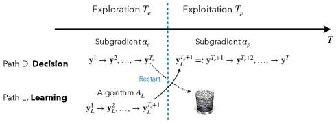
Figure 6: Two-path and two-phase decision for online linear programming

In this section, we present our results in a general framework. Our algorithm design contains two phases: exploration (E) and exploitation (P). See Figure 6 for an illustration.

Exploration.

This phase starts from time horizon $t=1$ to $t=T_{e}$. Two (first-order) algorithms simultaneously maintain and update two dual sequences, which we call Path Decision and Path Learning. Path D maintains sequence $\{\mathbf{y}^{t}\}$ that is used for decision, and for simplicity we restrict Path D to use subgradient update with stepsize $\alpha_{e}$

$$x^{t}={} \mathbb{I}\{c_{t}>\langle\mathbf{a}_{t},\mathbf{y}^{t}\rangle\}$$

$$\mathbf{y}^{t+1}={} [\mathbf{y}^{t}-\alpha_{e}(\mathbf{d}-\mathbf{a}_{t}x^{t})]_{+}.$$

From our discussion in Section A, subgradient has convergence rate $\theta=1/4$. In contrast, Path L should be equipped with a learning algorithm with $\theta\geq 1/4$, which aims to output the best possible $\mathbf{y}^{T_{e}+1}_{L}$ when the exploration phase ends. Our analysis allows $T_{e}=0$ or $T_{e}=T$ to encompass the analysis of traditional one-phase algorithms.

Exploitation.

At time horizon $T_{e}+1$, the online algorithm enters “exploitation” phase, where we no longer maintain Path L and restarts Path D with $\mathbf{y}^{T_{e}+1}_{L}$. In the exploitation phase, Path D still uses subgradient method but with a different stepsize $\alpha_{p}$ till the end of horizon $T$.

Table 4: Notations of algorithm design

Notation	Meaning
$\mathcal{A}_{L}$	Path L learning algorithm
$\theta$	Convergence rate of $\mathcal{A}_{L}$
$\alpha_{e}$	Stepsize of subgradient in exploration
$\alpha_{p}$	Stepsize of subgradient in exploitation
$\mathbf{y}^{t}$	$t$-th dual iteration for decision algorithm
$\mathbf{y}_{L}^{t}$	$t$-th dual iteration in exploration for learning algorithm $\mathcal{A}_{L}$
$T$	Total decision horizon $T$
$T_{e}$	Time of transition from exploration to exploitation
$T_{p}$	$T-T_{e}$

Our analysis is done in two steps. In B.1, we focus on the behavior of dual iterations in Path D. In B.2, we analyze the regret and constraint violation bounds for our two-phase algorithm. We show that given $\theta$, $(T_{e},\alpha_{e},\alpha_{p})$ can be optimally determined to improve algorithm performance.

B.1 Dual Convergence

In this section, we analyze the behavior of $\{\mathbf{y}^{t}\}$ along Path D, where iterate by $\mathbf{y}^{t+1}=[\mathbf{y}^{t}-\alpha_{t}(\mathbf{d}-\mathbf{a}_{t}x^{t})]_{+}$ and

1. before restart, we take stepsize $\alpha_{p}$

2. after restart from $\mathbf{y}^{T_{e}+1}$, we take stepsize $\alpha_{e}$

where $\mathbf{y}^{T_{e}+1}\in\Xi_{0}$. The following lemma characterizes almost sure boundedness of the dual sequence $\{\mathbf{y}^{t}\}$.

Lemma 11.

Assume that A1 to A6 hold. Let $\{\mathbf{y}^{t}\}$ be generated by Path D, then

$$\|\mathbf{y}^{t}\|\leq{} \frac{\bar{c}}{\underline{d}}+\frac{m(\bar{a}+\bar{d})^{2}\alpha_{e}}{2\underline{d}}+\alpha_{e}\sqrt{m}(\bar{a}+\bar{d}),\text{ for all }t\leq T_{e},$$

$$\|\mathbf{y}^{t}\|\leq{} \frac{\bar{c}}{\underline{d}}+\frac{m(\bar{a}+\bar{d})^{2}\alpha_{p}}{2\underline{d}}+\alpha_{p}\sqrt{m}(\bar{a}+\bar{d}),\text{ for all }t\geq T_{e}+1$$

almost surely. In other words, $\mathbf{y}^{t}\in\Xi_{1}$ for all $\alpha_{p}\leq\frac{2\underline{d}}{3m(\bar{a}+\bar{d})^{2}}$ almost surely.

The next lemma will be used to obtain a stronger dual convergence result for $\{\mathbf{y}^{t}\},t\geq T_{e}+1$.

Lemma 12.

Assume that A1 to A6 hold, then

$$\mathbb{E}[\|\mathbf{y}^{T+1}-\mathbf{y}^{\star}\|^{2}|\mathbf{y}^{T_{e}+1}]\leq\frac{\|\mathbf{y}^{T_{e}+1}_{e}-\mathbf{y}^{\star}\|^{2}}{\mu\alpha_{p}T_{p}}+\frac{m(\bar{a}+\bar{d})^{2}}{\mu}\alpha_{p}$$

Proof of Lemma 11.

The first relation follows immediately from Lemma 5 of [9] using $\mathbf{y}^{1}=\textbf{0}$, while the second relation uses the fact $\mathbf{y}^{T_{e}+1}=\mathbf{y}^{T_{e}+1}_{L}\in\Xi_{0}$ and that $\|\mathbf{y}^{T_{e}+1}\|\leq\frac{\bar{c}}{\underline{d}}$. To see $\mathbf{y}^{t}\in\Xi_{1}$, we successively deduce that, for $\alpha_{p}\leq\frac{2\underline{d}}{3m(\bar{a}+\bar{d})^{2}}$, that

$$\frac{m(\bar{a}+\bar{d})^{2}\alpha_{p}}{2\underline{d}}+\alpha_{p}\sqrt{m}(\bar{a}+\bar{d})=\frac{1}{3}+\frac{2\underline{d}}{3\sqrt{m}(\bar{a}+\bar{d})}\leq\frac{1}{3}+\frac{2(\bar{a}+\bar{d})}{3\sqrt{m}(\bar{a}+\bar{d})}\leq 1$$

and this completes the proof.

Proof of Lemma 12.

The result is a direct consequence of Lemma 6, where we consider $\mathbf{y}^{T_{e}+1}$ as the starting point.

B.2 Performance Analysis of Algorithm

In this section, we conduct the performance analysis of our algorithm. With the auxiliary results in hand, the proof focuses on finding a proper trade-off between $T_{e},\alpha_{p},\alpha_{d}$ based on $\theta$. To simplify notation, we define

$$\mathsf{R}\coloneqq\frac{\bar{c}}{\underline{d}}+\bigg{[}\frac{m(\bar{a}+\bar{d})^{2}}{2\underline{d}}+\sqrt{m}(\bar{a}+\bar{d})\bigg{]}\cdot\max\{\alpha_{e},\alpha_{p}\}$$ (21)

respectively and from Lemma 11 we know that $\|\mathbf{y}^{t}\|\leq\mathsf{R}$ almost surely. Though we have not formally chosen $\alpha_{e},\alpha_{p}$, they will be set such that $\mathsf{R}=\frac{\bar{c}}{\underline{d}}+o(1)=\mathcal{O}(1)$.

The following lemma analyzes the regret of the whole algorithm.

Lemma 13.

Assuming A1 to A6, we have

$$\mathbb{E}[r(\hat{\mathbf{x}})]\leq\frac{m(\bar{a}+\bar{d})^{2}\alpha_{e}}{2}T_{e}+\frac{m(\bar{a}+\bar{d})^{2}\alpha_{p}}{2}T_{p}+\frac{\mathsf{R}}{\alpha_{p}}\mathbb{E}[\|\mathbf{y}^{T_{e}+1}-\mathbf{y}^{\star}\|+\|\mathbf{y}^{T+1}-\mathbf{y}^{\star}\|].$$

The next lemma analyzes the constraint violation of the whole algorithm.

Lemma 14.

Assuming A1 to A6, we have

$$\mathbb{E}[v(\hat{\mathbf{x}})]\leq\frac{\mathsf{R}}{\alpha_{e}}+\frac{1}{\alpha_{p}}\mathbb{E}[\|\mathbf{y}^{T_{e}+1}-\mathbf{y}^{\star}\|+\|\mathbf{y}^{T+1}-\mathbf{y}^{\star}\|].$$

Putting things together, we take a trade-off between $T_{e},\alpha_{p},\alpha_{d}$ and get the following result.

Theorem 2.

Under the same assumptions as Lemma 13 as well as A7, let $\theta^{\prime}=\min\{\theta,1/2\}$. Then for all $T\geq\frac{36m(\bar{a}+\bar{d})^{2}}{\underline{d}}$. If we choose

$$T_{e}^{\star}=T^{\frac{1}{\theta^{\prime}+1}},\quad\alpha_{e}^{\star}=T^{-\frac{1}{2(\theta^{\prime}+1)}},\quad\alpha_{p}^{\star}=T^{-\frac{2\theta^{\prime}+1}{2(\theta^{\prime}+1)}},$$

Then

$$\mathbb{E}[r(\hat{\mathbf{x}})+v(\hat{\mathbf{x}})]\leq\mathcal{O}(T^{\frac{1}{2(\theta^{\prime}+1)}}).$$

Proof of Lemma 13.

We first deduce that

$$\mathbb{E}[r(\hat{\mathbf{x}})]={} \mathbb{E}[\langle\mathbf{c},\mathbf{x}^{\star}\rangle-\langle\mathbf{c},\hat{\mathbf{x}}\rangle]$$

$$={} \mathbb{E}[f_{T}(\mathbf{y}_{T}^{\star})-\langle\mathbf{c},\hat{\mathbf{x}}\rangle]$$ (22)

$$\leq{} \mathbb{E}[f_{T}(\mathbf{y}^{\star})-\langle\mathbf{c},\hat{\mathbf{x}}\rangle]$$ (23)

$$={} f(\mathbf{y}^{\star})-\mathbb{E}[\langle\mathbf{c},\hat{\mathbf{x}}\rangle]$$

$$\leq{} \mathbb{E}[f(\mathbf{y}^{t})-\langle\mathbf{c},\hat{\mathbf{x}}\rangle]$$

$$={} \sum_{t=1}^{T}\mathbb{E}[\langle\mathbf{d},\mathbf{y}^{t}\rangle+[c_{t}-\langle\mathbf{a}_{t},\mathbf{y}^{t}\rangle]_{+}-c_{t}x^{t}]$$ (24)

$$={} \sum_{t=1}^{T}\mathbb{E}[\langle\mathbf{d}-\mathbf{a}_{t}x_{t},\mathbf{y}^{t}\rangle],$$

where (22) uses strong duality of LP; (23) uses the fact $\mathbf{y}^{\star}$ is a feasible solution and that $\mathbf{y}_{T}^{\star}$ is the optimal solution to the sample LP; (24) uses the definition of $f(\mathbf{y})$ and that $(c_{t},\mathbf{a}_{t})$ are i.i.d. generated.

Recall that given $\alpha\in\{\alpha_{p},\alpha_{d}\}$,

$$\|\mathbf{y}^{t+1}\|^{2}-\|\mathbf{y}^{t}\|^{2}={} \|[\mathbf{y}^{t}-\alpha(\mathbf{d}-\mathbf{a}_{t}x^{t})]_{+}\|^{2}-\|\mathbf{y}^{t}\|^{2}$$

$$\leq{} \|\mathbf{y}^{t}-\alpha(\mathbf{d}-\mathbf{a}_{t}x^{t})\|^{2}-\|\mathbf{y}^{t}\|^{2}$$ (25)

$$={} -2\alpha\langle\mathbf{d}-\mathbf{a}_{t}x^{t},\mathbf{y}^{t}\rangle+\alpha^{2}\|\mathbf{d}-\mathbf{a}_{t}x^{t}\|^{2}$$

$$\leq{} -2\alpha\langle\mathbf{d}-\mathbf{a}_{t}x^{t},\mathbf{y}^{t}\rangle+m(\bar{a}+\bar{d})^{2}\alpha^{2},$$ (26)

where (25) uses $\|[\mathbf{x}]_{+}\|\leq\|\mathbf{x}\|$ and (26) uses A2, A3. A simple re-arrangement gives

$$\langle\mathbf{d}-\mathbf{a}_{t}x^{t},\mathbf{y}^{t}\rangle\leq\frac{m(\bar{a}+\bar{d})^{2}\alpha}{2}+\frac{\|\mathbf{y}^{t}\|^{2}-\|\mathbf{y}^{t+1}\|^{2}}{2\alpha}$$ (27)

Now we decompose regret according to two phases

$$\mathbb{E}[r(\hat{\mathbf{x}})]={} \sum_{t=1}^{T}\mathbb{E}[\langle\mathbf{d}-\mathbf{a}_{t}x_{t},\mathbf{y}^{t}\rangle]$$

$$={} \sum_{t=1}^{T_{e}}\mathbb{E}[\langle\mathbf{d}-\mathbf{a}_{t}x_{t},\mathbf{y}^{t}\rangle]+\sum_{t=T_{e}+1}^{T}\mathbb{E}[\langle\mathbf{d}-\mathbf{a}_{t}x_{t},\mathbf{y}^{t}\rangle]$$

$$=: r_{e}+r_{p}$$

and we bound two parts of regret respectively. For ${r_{e}}$, we have

$$r_{e}={} \sum_{t=1}^{T_{e}}\mathbb{E}[\langle\mathbf{d}-\mathbf{a}_{t}x_{t},\mathbf{y}^{t}\rangle]$$

$$\leq{} \frac{m(\bar{a}+\bar{d})^{2}\alpha_{e}}{2}T_{e}+\sum_{t=1}^{T_{e}}\frac{\|\mathbf{y}^{t}\|^{2}-\|\mathbf{y}^{t+1}\|^{2}}{2\alpha_{e}}$$ (28)

$$\leq{} \frac{m(\bar{a}+\bar{d})^{2}\alpha_{e}}{2}T_{e}+\frac{\|\mathbf{y}^{1}\|^{2}-\mathbb{E}[\|\mathbf{y}^{T_{e}+1}\|^{2}]}{2\alpha_{e}}$$ (29)

$$\leq{} \frac{m(\bar{a}+\bar{d})^{2}\alpha_{e}}{2}T_{e},$$

where (28) uses relation (27) and in (29) we used $\mathbf{y}^{1}=\textbf{0}$. For $r_{p}$, we have

$$r_{p}={} \sum_{t=T_{e}+1}^{T}\mathbb{E}[\langle\mathbf{d}-\mathbf{a}_{t}x_{t},\mathbf{y}^{t}\rangle]$$

$$\leq{} \frac{m(\bar{a}+\bar{d})^{2}\alpha_{p}}{2}T_{p}+\sum_{t=T_{e}+1}^{T}\frac{\mathbb{E}[\|\mathbf{y}^{t}\|^{2}]-\mathbb{E}[\|\mathbf{y}^{t+1}\|^{2}]}{2\alpha_{p}}$$ (30)

$$={} \frac{m(\bar{a}+\bar{d})^{2}\alpha_{p}}{2}T_{p}+\frac{\mathbb{E}[\|\mathbf{y}^{T_{e}+1}\|^{2}]-\mathbb{E}[\|\mathbf{y}^{T+1}\|^{2}]}{2\alpha_{p}}$$

$$={} \frac{m(\bar{a}+\bar{d})^{2}\alpha_{p}}{2}T_{p}+\frac{\mathbb{E}[\langle\mathbf{y}^{T_{e}+1}+\mathbf{y}^{T+1},\mathbf{y}^{T_{e}+1}-\mathbf{y}^{T+1}\rangle]}{2\alpha_{p}}$$ (31)

$$\leq{} \frac{m(\bar{a}+\bar{d})^{2}\alpha_{p}}{2}T_{p}+\frac{\mathsf{R}}{\alpha_{p}}\mathbb{E}[\|\mathbf{y}^{T_{e}+1}-\mathbf{y}^{T+1}\|]$$ (32)

$$={} \frac{m(\bar{a}+\bar{d})^{2}\alpha_{p}}{2}T_{p}+\frac{\mathsf{R}}{\alpha_{p}}\mathbb{E}[\|\mathbf{y}^{T_{e}+1}-\mathbf{y}^{\star}\|+\|\mathbf{y}^{T+1}-\mathbf{y}^{\star}\|],$$ (33)

where (30) again uses relation (27); (32) uses the Cauchy’s inequality

$$\langle\mathbf{y}^{T_{e}+1}+\mathbf{y}^{T_{e}+1},\mathbf{y}^{T_{e}+1}-\mathbf{y}^{T+1}\rangle\leq\|\mathbf{y}^{T_{e}+1}+\mathbf{y}^{T+1}\|\cdot\|\mathbf{y}^{T_{e}+1}-\mathbf{y}^{T+1}\|$$

and almost sure boundedness of iterations derived from Lemma 11; (33) is obtained from triangle inequality

$$\|\mathbf{y}^{T_{e}+1}+\mathbf{y}^{T+1}\|\leq{} \|\mathbf{y}^{T+1}\|+\|\mathbf{y}^{T_{e}+1}\|\leq{}2\mathsf{R}$$

$$\|\mathbf{y}^{T_{e}+1}-\mathbf{y}^{T+1}\|={} \|\mathbf{y}^{T_{e}+1}-\mathbf{y}^{\star}+\mathbf{y}^{\star}-\mathbf{y}^{T+1}\|\leq\|\mathbf{y}^{T_{e}+1}-\mathbf{y}^{\star}\|+\|\mathbf{y}^{T+1}-\mathbf{y}^{\star}\|.$$

Summing up two bounds on $r_{e}$ and $r_{p}$ completes the proof.

Proof of Lemma 14.

For constraint violation, recall that

$$\mathbb{E}[v(\hat{\mathbf{x}})]=\mathbb{E}[\|[\mathbf{A}\hat{\mathbf{x}}-\mathbf{b}]_{+}\|]=\mathbb{E}\bigg{[}\bigg{\|}\bigg{[}\sum_{t=1}^{T}(\mathbf{a}_{t}x^{t}-\mathbf{d})]_{+}\bigg{\|}\bigg{]}$$

and that

$$\mathbf{y}^{t+1}=[\mathbf{y}^{t+1}-\alpha(\mathbf{d}-\mathbf{a}_{t}x^{t})]_{+}\geq\mathbf{y}^{t}-\alpha(\mathbf{d}-\mathbf{a}_{t}x^{t}).$$

A re-arrangement gives, for $\alpha\in\{\alpha_{e},\alpha_{p}\}$, that

$$\mathbf{a}_{t}x^{t}\leq\mathbf{d}+\frac{1}{\alpha}(\mathbf{y}^{t+1}-\mathbf{y}^{t}).$$ (34)

Now we decompose $\sum_{t=1}^{T}(\mathbf{a}_{t}x^{t}-\mathbf{d})$ by

$$\sum_{t=1}^{T}(\mathbf{a}_{t}x^{t}-\mathbf{d})={} \sum_{t=1}^{T_{e}}(\mathbf{a}_{t}x^{t}-\mathbf{d})+\sum_{t=T_{e}+1}^{T}(\mathbf{a}_{t}x^{t}-\mathbf{d})$$

$$\leq{} \frac{1}{\alpha_{e}}\sum_{t=1}^{T_{e}}(\mathbf{y}^{t+1}-\mathbf{y}^{t})+\frac{1}{\alpha_{p}}\sum_{t=T_{e}+1}^{T}(\mathbf{y}^{t+1}-\mathbf{y}^{t})$$ (35)

$$={} \frac{1}{\alpha_{e}}(\mathbf{y}^{T_{e}+1}-\mathbf{y}^{1})+\frac{1}{\alpha_{p}}(\mathbf{y}^{T+1}-\mathbf{y}^{T_{e}+1})$$

$$={} \frac{1}{\alpha_{e}}\mathbf{y}^{T_{e}+1}+\frac{1}{\alpha_{p}}(\mathbf{y}^{T+1}-\mathbf{y}^{T_{e}+1}),$$

where (35) uses (34) and we deduce that

$$\mathbb{E}[\|[\mathbf{A}\hat{\mathbf{x}}-\mathbf{b}]_{+}\|]\leq{} \mathbb{E}\Big{[}\Big{\|}\frac{1}{\alpha_{e}}\mathbf{y}^{T_{e}+1}+\frac{1}{\alpha_{p}}(\mathbf{y}^{T+1}-\mathbf{y}^{T_{e}+1})\Big{\|}\Big{]}$$

$$\leq{} \frac{1}{\alpha_{e}}\mathbb{E}[\|\mathbf{y}^{T_{e}+1}\|]+\frac{1}{\alpha_{p}}\mathbb{E}[\|\mathbf{y}^{T+1}-\mathbf{y}^{T_{e}+1}\|]$$

$$\leq{} \frac{\mathsf{R}}{\alpha_{e}}+\frac{1}{\alpha_{p}}\mathbb{E}[\|\mathbf{y}^{T_{e}+1}-\mathbf{y}^{\star}\|+\|\mathbf{y}^{T+1}-\mathbf{y}^{\star}\|],$$ (36)

where (36) again uses triangle inequality and this completes the proof.

Proof of Theorem 2.

For all $T\geq\frac{36m(\bar{a}+\bar{d})^{2}}{\underline{d}}$, we know

$$T\geq\exp\big{(}\tfrac{2\theta^{\prime}+1}{2(\theta^{\prime}+1)}\big{)}\tfrac{3m(\bar{a}+\bar{d})^{2}}{2\underline{d}}$$

since $\tfrac{2\theta^{\prime}+1}{2(\theta^{\prime}+1)}<3<\log 24$. Therefore $\alpha_{p}\leq\tfrac{2\underline{d}}{3m(\bar{a}+\bar{d})^{2}}$ and by Lemma 11 we know $\mathbf{y}^{t}\in\Xi_{1}$ almost surely.

Next we consider the sum of regret and violation by summing up Lemma 13 and Lemma 14.

$$\mathbb{E}[r(\hat{\mathbf{x}})+v(\hat{\mathbf{x}})]\leq{} \frac{m(\bar{a}+\bar{d})^{2}\alpha_{e}}{2}T_{e}+\frac{m(\bar{a}+\bar{d})^{2}\alpha_{p}}{2}T_{p}+\frac{\mathsf{R}}{\alpha_{p}}\mathbb{E}[\|\mathbf{y}^{T_{e}+1}-\mathbf{y}^{\star}\|+\|\mathbf{y}^{T+1}-\mathbf{y}^{\star}\|]$$

$$+\frac{\mathsf{R}}{\alpha_{e}}+\frac{1}{\alpha_{p}}\mathbb{E}[\|\mathbf{y}^{T_{e}+1}-\mathbf{y}^{\star}\|+\|\mathbf{y}^{T+1}-\mathbf{y}^{\star}\|]$$

$$={} V_{e}+V_{p},$$

where we define

$$V_{e}:={} \frac{m(\bar{a}+\bar{d})^{2}\alpha_{e}}{2}T_{e}+\frac{\mathsf{R}}{\alpha_{e}}$$

$$V_{p}:={} \frac{m(\bar{a}+\bar{d})^{2}\alpha_{p}}{2}T_{p}+\frac{\mathsf{R}+1}{\alpha_{p}}\mathbb{E}[\|\mathbf{y}^{T_{e}+1}-\mathbf{y}^{\star}\|+\|\mathbf{y}^{T+1}-\mathbf{y}^{\star}\|].$$

Next we invoke A7, where we have, with probability $1-1/T$, that

$$\mathbb{E}[\|\mathbf{y}^{T_{e}+1}-\mathbf{y}^{\star}\|]\leq\frac{c_{1}+c_{2}\log T_{e}}{T_{e}^{\theta}}\leq\frac{c_{1}+c_{2}\log T}{T_{e}^{\theta}}$$

Denote the event $\mathbb{E}[\|\mathbf{y}^{T_{e}+1}-\mathbf{y}^{\star}\|]\leq\frac{c_{1}+c_{2}\log T}{T_{e}^{\theta}}$ to be $E$, we have, by Lemma 12 that

$$\mathbb{E}[\|\mathbf{y}^{T_{e}+1}-\mathbf{y}^{\star}\|]={} \mathbb{E}[\|\mathbf{y}^{T_{e}+1}-\mathbf{y}^{\star}\||E]\cdot\mathbb{P}\{E\}+\mathbb{E}[\|\mathbf{y}^{T_{e}+1}-\mathbf{y}^{\star}\||\bar{E}]\cdot\mathbb{P}\{\bar{E}\}$$

$$\leq{} \mathbb{E}[\|\mathbf{y}^{T_{e}+1}-\mathbf{y}^{\star}\||E]+\mathbb{E}[\|\mathbf{y}^{T_{e}+1}-\mathbf{y}^{\star}\||\bar{E}]\cdot\mathbb{P}\{\bar{E}\}$$

$$\leq{} \frac{c_{1}+c_{2}\log T}{T_{e}^{\theta}}+\frac{2\mathsf{R}}{T}$$ (37)

$$\cong{} \frac{\log T}{T_{e}^{\theta}}+\frac{2\mathsf{R}}{T},$$

where (37) uses Lemma 11 and Lemma 1. Similarly we can deduce that

$$\mathbb{E}[\|\mathbf{y}^{T+1}-\mathbf{y}^{\star}\|]={} \mathbb{E}[\|\mathbf{y}^{T+1}-\mathbf{y}^{\star}\||E]\cdot\mathbb{P}\{E\}+\mathbb{E}[\|\mathbf{y}^{T+1}-\mathbf{y}^{\star}\||\bar{E}]\cdot\mathbb{P}\{\bar{E}\}$$

$$\leq{} \mathbb{E}[\|\mathbf{y}^{T+1}-\mathbf{y}^{\star}\||E]+\mathbb{E}[\|\mathbf{y}^{T+1}-\mathbf{y}^{\star}\||\bar{E}]\cdot\mathbb{P}\{\bar{E}\}$$

$$\leq{} \tfrac{c_{1}+c_{2}\log T}{\sqrt{\mu}\sqrt{T_{p}}T_{e}^{\theta}}\alpha_{p}^{-1/2}+\sqrt{\tfrac{m(\bar{a}+\bar{d})^{2}}{\mu}}\alpha_{p}^{1/2}+\tfrac{2\mathsf{R}}{T}$$ (38)

$$\cong{} \tfrac{\log T}{\sqrt{\mu}\sqrt{T_{p}}T_{e}^{\theta}}\alpha_{p}^{-1/2}+\sqrt{\tfrac{m}{\mu}}\alpha_{p}^{1/2}+\tfrac{2\mathsf{R}}{T}$$

where in (38) we invoke Lemma (12) and the inequality $\sqrt{a+b}\leq\sqrt{a}+\sqrt{b}$. Then we have

$$V_{p}\lesssim\frac{m(\bar{a}+\bar{d})^{2}\alpha_{p}}{2}T_{p}+(\log T)T_{e}^{-\theta}\alpha_{p}^{-1}+\frac{\log T}{\sqrt{\mu}}T_{p}^{-1/2}T_{e}^{-\theta}\alpha_{p}^{-3/2}+\sqrt{\frac{m}{\mu}}\alpha_{p}^{-1/2}+\frac{4\mathsf{R}}{\alpha_{p}T}.$$

And notice that $\alpha_{e}$ only appears in

$$V_{e}=\frac{m(\bar{a}+\bar{d})^{2}\alpha_{e}}{2}T_{e}+\frac{\mathsf{R}}{\alpha_{e}}$$

and $\alpha_{e}=\sqrt{\frac{2\mathsf{R}}{m(\bar{a}+\bar{d})^{2}T_{e}}}=\mathcal{O}(\frac{1}{\sqrt{T_{e}}})$ minimizes $V_{p}$, giving $V_{p}=\mathcal{O}(T_{e}^{1/2})$. Therefore, we fix $\alpha_{e}=T_{e}^{-1/2}$ and put all the things together to choose $T_{p},\alpha_{e},\alpha_{p}$. Ignoring all the constants and $\log T$ terms, we have

$$V_{p}+V_{e}\lesssim T_{e}^{1/2}+T_{p}\alpha_{p}+T_{e}^{-\theta}\alpha_{p}^{-1}+T_{p}^{-1/2}T_{e}^{-\theta}\alpha_{p}^{-3/2}+\alpha_{p}^{-1/2}+\alpha_{p}^{-1}T^{-1}$$

We now do case analysis.

Case 1.

If $\theta=0$, then learning algorithm does not converge. $T_{p}\alpha_{p}+\alpha_{p}^{-1}\geq 2\sqrt{T_{p}}$ and $\sqrt{T_{e}}+\sqrt{T_{p}}\geq\sqrt{T_{e}+T_{p}}=\sqrt{T}$. In this case choosing $T_{e}=T,T_{p}=0,\alpha_{e}=\sqrt{T}$ gives

$$V_{p}+V_{e}\leq\mathcal{O}(\sqrt{T}).$$

Case 2.

If $0<\theta<1/2$, then learning algorithm converges. Without loss of generality, we take $T_{e}=T^{\beta},\beta\in(0,1)$ and successively deduce that

$$V_{p}+V_{e}$$

$$\lesssim{} T_{e}^{1/2}+T_{p}\alpha_{p}+T_{e}^{-\theta}\alpha_{p}^{-1}+T_{p}^{-1/2}T_{e}^{-\theta}\alpha_{p}^{-3/2}+\alpha_{p}^{-1/2}+\alpha_{p}^{-1}T^{-1}$$

$$\cong{} T^{\beta/2}+T(1-T_{e}T^{-1})\alpha_{p}+T^{-\theta\beta}\alpha_{p}^{-1}+T^{-1/2}(1-T_{e}T^{-1})^{-1/2}T^{-\theta\beta}\alpha_{p}^{-3/2}+\alpha_{p}^{-1/2}+\alpha_{p}^{-1}T^{-1}$$

$$\cong{} T^{\beta/2}+\alpha_{p}T+T^{-\theta\beta}\alpha_{p}^{-1}+\alpha_{p}^{-3/2}T^{-1/2-\beta\theta}+\alpha_{p}^{-1/2}+\alpha_{p}^{-1}T^{-1}$$

Now assume $\alpha_{p}=T^{-\lambda}$, we have

$$V_{p}+V_{e}\lesssim T^{\beta/2}+T^{1-\lambda}+T^{\lambda-\theta\beta}+T^{\frac{3}{2}\lambda-1/2-\beta\theta}+T^{\frac{\lambda}{2}}+T^{\lambda-1}$$

and this reduces to an optimization problem

$$\min_{\lambda,\beta} \max\{\frac{\beta}{2},1-\lambda,\lambda-\theta\beta,\frac{3}{2}\lambda-\frac{1}{2}-\beta\theta,\frac{\lambda}{2},\lambda-1\}$$

subject to $$0\leq\beta\leq 1$$

$$\lambda\geq 0$$

and solving the problem gives the following parameter setting

$$\beta^{\star}(\theta)={} \tfrac{1}{\theta+1}$$

$$\lambda^{\star}(\theta)={} 1-\tfrac{1}{2(\theta+1)}$$

$$\alpha_{e}^{\star}(\theta)={} T^{-\frac{1}{2(\theta+1)}}$$

$$\alpha_{p}^{\star}(\theta)={} T^{-\frac{2\theta+1}{2(\theta+1)}}$$

$$T_{e}^{\star}(\theta)={} T^{\frac{1}{\theta+1}}$$

$$V_{p}+V_{e}\lesssim{} \mathcal{O}(T^{\frac{1}{2(\theta+1)}})$$

Case 3.

If $\theta>1/2$, we have $\alpha_{e}^{\star}=T^{-1/3},\alpha_{p}^{\star}=T^{-2/3},T_{e}^{\star}=T^{2/3}$ and $V_{p}+V_{e}=\mathcal{O}(T^{1/3})$.

Putting all the results together, we have

$$\theta^{\prime}={} \min\{\theta,1/2\}$$

$$T_{e}^{\star}(\theta)={} T^{\frac{1}{\theta^{\prime}+1}}$$

$$\alpha_{e}^{\star}(\theta)={} T^{-\frac{1}{2(\theta^{\prime}+1)}}$$

$$\alpha_{p}^{\star}(\theta)={} T^{-\frac{2\theta^{\prime}+1}{2(\theta^{\prime}+1)}}$$

and $V_{p}+V_{e}=\mathcal{O}(T^{\frac{1}{2(\theta^{\prime}+1)}})$. Adding back $\log T$ terms, this completes the proof.

Appendix C Proof of Main Results in Section 3

C.1 Proof of Proposition 1

Invoke Theorem 2, plug in $\theta^{\prime}=\min\{\theta,1/2\}$ and this completes the proof.

C.2 Proof of Proposition 2

First, we establish the update rule formula for $\mathbb{E}[y^{t+1}]$ in terms of $\mathbb{E}[y^{t}]$. Specifically, we have

$$\mathbb{E}[y^{t+1}]={} \mathbb{E}[[y^{t}-\tfrac{1}{t}(\tfrac{1}{2}-\mathbb{I}\{c_{t}>y^{t}\})]_{+}]$$ (39)

$$\geq{} \mathbb{E}[y^{t}-\tfrac{1}{t}(\tfrac{1}{2}-\mathbb{I}\{c_{t}>y^{t}\})]$$ (40)

$$\geq{} \mathbb{E}[y^{t}-\tfrac{1}{t}y^{t}+\tfrac{1}{2t}]$$ (41)

where (39) is obtained by the update rule of subgradient, (40) uses Jensen’s inequality, and (41) is obtained by the fact that $c_{t}$ is independent of $y^{t}$ and it is drawn uniformly from $[0,1]$. Indeed, we have

$$\mathbb{E}[\mathbb{I}\{c_{t}>y^{t}\}]=\mathbb{E}[\mathbb{E}[\mathbb{I}\{c_{t}>y^{t}\}|y^{t}]]=\mathbb{E}[\textstyle\int_{0}^{1}\mathbb{I}\{c>y^{t}\}\mathrm{d}c|y^{t}]=\mathbb{E}[1-y^{t}].$$

Subtracting $t/2$ from both sides and multiplying both sides the the inequality by $t$, we have

$$t(\mathbb{E}[y^{t+1}]-\tfrac{1}{2})\geq(t-1)(\mathbb{E}[y^{t}]-\tfrac{1}{2}),\quad\text{for all $t=1,\dots,T$.}$$

Next we condition on the value of $y^{t_{0}}$ and

$$t(\mathbb{E}[y^{t+1}|y^{t_{0}}]-\tfrac{1}{2})\geq(t_{0}-1)(y^{t_{0}}-\tfrac{1}{2}).$$ (42)

Thus, given $y^{t_{0}}>y^{\star}+\tfrac{1}{\sqrt{T}}=\frac{1}{2}+\tfrac{1}{\sqrt{T}}$ for some $t_{0}$, we have

$$t(\mathbb{E}[y^{t+1}|y^{t_{0}}]-\tfrac{1}{2})\geq(t_{0}-1)(y^{t_{0}}-\tfrac{1}{2})\geq\tfrac{t_{0}-1}{\sqrt{T}},$$ (43)

As a result, when $t_{0}\geq\tfrac{T}{10}+1$, (43) implies

$$\mathbb{E}[y^{t+1}|y^{t_{0}}]\geq\tfrac{1}{2}+\tfrac{t_{0}-1}{t\times\sqrt{T}}\geq\tfrac{1}{2}+\tfrac{1}{10\sqrt{T}},$$

since we assume $t_{0}\geq T/10+1$. This completes the proof.

C.3 Proof of Proposition 3

Based on rakhlin2011making, there exists some universal constant $c>0$ such that with probability no less than $1-1/T^{4}$, $|y^{t}-y^{\star}|\leq c\log T/\sqrt{T}$ for all $t\geq t_{0}$, where $y^{\star}=\frac{1}{2}$ and $t_{0}=\mathcal{O}(\log T)$. Thus, without loss of generality, we assume

$$y^{t}\in[\tfrac{1}{4},\tfrac{3}{4}],\text{ and }y^{t+1}=y^{t}-\tfrac{1}{t}(\tfrac{1}{2}-\mathbb{I}\{c_{t}>y^{t}\})$$ (44)

for all $t\geq t_{0}$ by setting a new random initialization $y^{t_{0}}\in[1/4,3/4]$ and ignoring the all decision steps before the $t_{0}$ step. In the following, we show that Algorithm 1 with SGD and known $\mu$ must have $\Omega(T^{1/2})$ regret or constraint violation for any initialization $y^{t_{0}}$. We first calculate $\mathbb{E}[y^{t}-\frac{1}{2}]$ and $\mathbb{E}[(y^{t}-\frac{1}{2})^{2}]$ similar to the proof of Proposition 2. Specifically, for $\mathbb{E}[y^{t}-1/2]$, we have

$$\mathbb{E}[y^{t+1}|y^{t}]=\big{(}1-\frac{1}{t}\big{)}y^{t}+\frac{1}{2t},$$

which implies

$$\mathbb{E}[y^{t+1}-\tfrac{1}{2}|y^{t_{0}}]=\frac{t_{0}-1}{t}(y^{1}-\tfrac{1}{2})+\tfrac{1}{2},$$ (45)

Also, similarly, for $\mathbb{E}[(y^{t}-1/2)^{2}]$ we have under assumption (44)

$$\mathbb{E}[(y^{t+1}-\tfrac{1}{2})^{2}|y^{t}] =\mathbb{E}[(y^{t}-\tfrac{1}{t}(\tfrac{1}{2}-\mathbb{I}\{c_{t}>y^{t}\})-\tfrac{1}{2})^{2}|y^{t}]$$

$$=(1-\tfrac{1}{t})^{2}(y^{t}-\tfrac{1}{2})^{2}+\tfrac{1}{4t^{2}}-\tfrac{1}{t^{2}}(y^{t}-\tfrac{1}{2})^{2}$$

$$\geq(1-\tfrac{1}{t})^{2}(y^{t}-\tfrac{1}{2})^{2}+\tfrac{1}{4t^{2}}-\tfrac{c}{t^{3}},$$

which implies

$$\mathbb{E}[(y^{t+1}-\tfrac{1}{2})^{2}|y^{t}]\geq\frac{(t_{0}-1)^{2}}{t^{2}}(y^{t_{0}}-\tfrac{1}{2})^{2}+\frac{1}{4t}-\frac{c\log t+t_{0}}{t^{2}}.$$ (46)

Combining (45) and (46), we then can compute

$$\mathbb{E}\Big{[}\Big{(}\sum\limits_{t=t_{0}}^{T}\mathbb{I}{\{c_{t}>y^{t}\}}-\frac{T-t_{0}+1}{2}\Big{)}^{2}\Big{]} =\sum\limits_{t=t_{0}}^{T}\mathbb{E}[(\mathbb{I}{\{c_{t}>y^{t}\}}-\tfrac{1}{2})^{2}]+2\sum\limits_{t_{0}\leq i<j\leq T}\mathbb{E}[(\mathbb{I}{\{c_{j}>y^{j}\}}-\tfrac{1}{2})(\mathbb{I}{\{c_{i}>y^{i}\}}-\tfrac{1}{2})]$$

$$=\frac{T-t_{0}}{4}+2\sum\limits_{t_{0}\leq i<j\leq T}\mathbb{E}[(\mathbb{I}{\{c_{j}>y^{j}\}}-\tfrac{1}{2})(\mathbb{I}{\{c_{i}>y^{i}\}}-\tfrac{1}{2})]$$

$$=\frac{T-t_{0}}{4}+2\sum\limits_{t_{0}\leq i<j\leq T}\frac{i-1}{j-1}\mathbb{E}[(y^{i}-\tfrac{1}{2})^{2}]-\frac{i-1}{4i(j-1)}$$ (47)

$$\geq\frac{T-t_{0}}{4}-2\sum\limits_{t_{0}\leq i<j\leq T}\frac{c\log T+t_{0}}{(i-1)^{2}}$$

$$=\Omega(T).$$

In addition, since $|y^{t}-\tfrac{1}{2}|\leq\tfrac{c}{\sqrt{T}}$, by Hoeffding’s inequality, we have with probability no less than $1-\tfrac{1}{T^{2}}$

$$\Big{|}\sum\limits_{t=t_{0}}^{T}\mathbb{I}{\{c_{t}>y^{t}\}}-\frac{T-t_{0}+1}{2}\Big{|}=\mathcal{O}(\sqrt{T}\log T).$$

Consequently, by (C.3), we have

$$\mathbb{E}\Big{[}\Big{|}\sum\limits_{t=t_{0}}^{T}\mathbb{I}{\{c_{t}>y^{t}\}}-\frac{T-t_{0}+1}{2}\Big{|}\Big{]}=\Omega(\sqrt{T}/\log T).$$ (48)

This is the summation of constraint violation and constraint (resource) leftover, and thus, the summation of constraint violation and the regret must be no less than $\Omega(\sqrt{T}/\log T)$.

C.4 Proposition of Disability in Mistake Correction

In this section we still consider the multi-secretary problem (12), and we show that other algorithms listed in Table 2 with small stepsize also suffer from slow updating. In particular, Lemma 15 reveals that all gradient-descent-based algorithms listed in with high estimation accuracy and low learning rate can change no more than $\mathcal{O}(\tfrac{1}{T^{1/2}})$ within $\mathcal{O}(T^{\alpha})$ steps for all $\alpha\in(0,1)$.

Lemma 15.

Denote $y^{t}$ as the estimated dual price for the online secretary problem (12) at time $t$. Suppose (i) $|y^{t+1}-y^{t}|\leq\tfrac{1}{t}$, (ii) $\mathbb{E}[|y^{t}-y^{\star}|]\leq\tfrac{1}{t}$, and (iii) $y_{t}\leq 1$ for all $t=1,\dots,T$. Then, with probability no less than $1-\tfrac{2}{T^{3}}$,

$$|y^{t}-y^{t+k}|\leq\frac{2\sqrt{k}}{t}\cdot\log T\leq\frac{8\sqrt{k}}{T}\cdot\log T$$

for all $t\geq\tfrac{T}{2}$ and $0\leq k\leq T-t$.

Here, the condition assumed in Lemma 15 are abstracted from algorithms listed in Table 2: Condition (i) assumes that the learning rate is $\mathcal{O}(1/t)$; Condition (ii) assumes the estimation error of the optimal dual price can be bounded by $1/t$, which correspond to the convergence rate of optimizing strongly convex functions with stochastic gradient descent algorithms; Condition (iii) assumes that bounteousness of the estimated dual price. These conditions are satisfied by fast algorithms in Table 2 regardless of some universal constants.

Proof of Lemma 15. This is a direct application of Hoeffding’s inequality. Specifically, based on Hoeffding’s inequality, during steps $t$ to $t+k$, there are $\tfrac{1}{2}k\pm 2\sqrt{k}\log T$ acceptances and rejections. As a result, we have

$$|y^{t+k}-y^{t}|\leq\sum\limits_{s=t}^{t+\mathcal{O}(\sqrt{k})}\frac{1}{s}=\frac{4\sqrt{k}\log T}{t}.$$

Plugging in $t\geq\tfrac{T}{2}$, we complete the proof.

Appendix D Proof of Main Results in Section 4

The main results in the paper can be directly obtained as special cases of Theorem 2.

D.1 Proof of Lemma 2

In view of Lemma 13, we complete the proof.

D.2 Proof of Lemma 3

In view of Lemma 14, we complete the proof.

D.3 Proof of Theorem 1

In view of Theorem 2, we complete the proof by taking $\theta=\{0,\frac{1}{4},\frac{1}{2}\}$ respectively.

Appendix E Additional Experiments

In this section, we provide some supplementary experiments to further demonstrate the superior performance of our proposed framework. We still evaluate the performance of the two instances of the proposed framework, i.e., M1 and M2, and compare them with the no-exploration algorithm M0.

E.1 More Choices of $m$

In this subsection, we focus on the case that there are more than one type of resources. To demonstrate, we let $m=5$. We conduct experiments on $4$ distributions. The first $3$ distributions are generated in the same way as those in Section 5.1. The last distribution is generated as follows. We sample $c_{t}$ i.i.d. from uniform distribution $\mathcal{U}[0,5]$, and sample $a_{it}$ i.i.d. such that $a_{it}-5$ follows the beta distribution $\mathcal{B}(1,8)$. Each $d_{i}$ is still sampled i.i.d. from uniform distribution $\mathcal{U}[1/3,2/3]$. Note that all distributions satisfy Assumption A1 to A6.

The results are presented in Figure 7, and in the same way as Figure 3, with the only difference that we plot the first coordinate $\mathbf{y}^{t}_{1}$ to demonstrate the convergence behavior of the sequence $\{\mathbf{y}^{t}\}_{t=1}^{T}$. It clearly shows that, over all $4$ distributions, M1 and M2 has better order of regret and constraint violation than M0, and the dual solution sequence of M1 and M2 converge much faster than the one of M0. This demonstrates the superior and robust performance of our proposed framework.

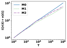
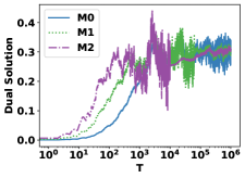
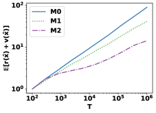
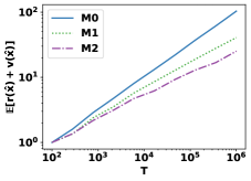
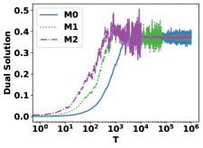
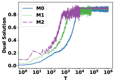
Figure 7: Growth of normalized $r(\hat{\mathbf{x}})+v(\hat{\mathbf{x}})$ and dual convergence of tested algorithms. Each pair of the left figure and the right figure is plotted based on the experiment on the same distribution.

E.2 More Distributions Violating Assumptions

In this subsection, we provide more experiments on distributions that violate the assumptions in Section 2. We generate $2$ different distributions, and take $m=1$. For the first distribution, we generate $c_{t}$ i.i.d. according to the uniform distribution $\mathcal{U}[1,6]$, and $a_{it}$ i.i.d. such that $a_{it}-3$ satisfies exponential distribution with parameter $m$. For the second distribution, we consider the discrete distribution. Specifically, we randomly generate $5$ different pairs of $(c_{t},\mathbf{a}_{t})$. Each $a_{it}$ is sampled i.i.d. from normal distribution $\mathcal{N}(1,2)$, and each $c_{t}=\sum_{i=1}^{m}a_{it}-\varepsilon_{t}$ with $\varepsilon_{t}$ from $\mathcal{U}[0,m]$. After obtaining these pairs of $\{(c_{t},\mathbf{a}_{t})\}$, at each time period $t$, we sample $(c_{t},\mathbf{a}_{t})$ from them with the same probability. Figure 8 plots the growth of normalized $r+v$ and the convergence behavior of $\{y^{t}\}_{t=1}^{T}$. It shows that even the assumptions are violated, M1 and M2 still enjoy better performance than M0.

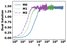
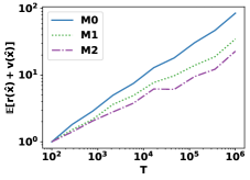
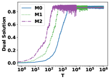
Figure 8: Growth of normalized $r(\hat{\mathbf{x}})+v(\hat{\mathbf{x}})$ and dual convergence of tested algorithms when the assumptions are violated. Each pair of the left figure and the right figure is plotted based on the experiment on the same distribution.

plain olp.bib

References

- [1] Shipra Agrawal, Zizhuo Wang, and Yinyu Ye. A dynamic near-optimal algorithm for online linear programming. Operations Research, 62(4):876–890, 2014.
- [2] Alessandro Arlotto and Itai Gurvich. Uniformly bounded regret in the multisecretary problem. Stochastic Systems, 9(3):231–260, 2019.
- [3] Santiago R Balseiro, Omar Besbes, and Dana Pizarro. Survey of dynamic resource-constrained reward collection problems: Unified model and analysis. Operations Research, 2023.
- [4] Santiago R Balseiro, Haihao Lu, and Vahab Mirrokni. The best of many worlds: Dual mirror descent for online allocation problems. Operations Research, 2022.
- [5] Santiago R Balseiro, Haihao Lu, Vahab Mirrokni, and Balasubramanian Sivan. From online optimization to PID controllers: Mirror descent with momentum. arXiv preprint arXiv:2202.06152, 2022.
- [6] Robert L Bray. Logarithmic regret in multisecretary and online linear programming problems with continuous valuations. arXiv e-prints, pages arXiv–1912, 2019.
- [7] Guanting Chen, Xiaocheng Li, and Yinyu Ye. An improved analysis of lp-based control for revenue management. Operations Research, 2022.
- [8] Zaiyi Chen, Yi Xu, Enhong Chen, and Tianbao Yang. Sadagrad: Strongly adaptive stochastic gradient methods. In International Conference on Machine Learning, pages 913–921. PMLR, 2018.
- [9] Wenzhi Gao, Dongdong Ge, Chunlin Sun, and Yinyu Ye. Solving linear programs with fast online learning algorithms. In International Conference on Machine Learning, pages 10649–10675. PMLR, 2023.
- [10] Guillaume Garrigos and Robert M Gower. Handbook of convergence theorems for (stochastic) gradient methods. arXiv preprint arXiv:2301.11235, 2023.
- [11] Hameed Hussain, Saif Ur Rehman Malik, Abdul Hameed, Samee Ullah Khan, Gage Bickler, Nasro Min-Allah, Muhammad Bilal Qureshi, Limin Zhang, Wang Yongji, Nasir Ghani, et al. A survey on resource allocation in high performance distributed computing systems. Parallel Computing, 39(11):709–736, 2013.
- [12] Jiashuo Jiang, Will Ma, and Jiawei Zhang. Degeneracy is OK: Logarithmic Regret for Network Revenue Management with Indiscrete Distributions. arXiv, 2022.
- [13] Naoki Katoh and Toshihide Ibaraki. Resource allocation problems. Handbook of Combinatorial Optimization: Volume1–3, pages 905–1006, 1998.
- [14] Thomas Kesselheim, Andreas Tönnis, Klaus Radke, and Berthold Vöcking. Primal beats dual on online packing lps in the random-order model. In Proceedings of the forty-sixth annual ACM symposium on Theory of computing, pages 303–312, 2014.
- [15] Xiaocheng Li, Chunlin Sun, and Yinyu Ye. Simple and fast algorithm for binary integer and online linear programming. Advances in Neural Information Processing Systems, 33:9412–9421, 2020.
- [16] Xiaocheng Li and Yinyu Ye. Online linear programming: Dual convergence, new algorithms, and regret bounds. Operations Research, 70(5):2948–2966, 2022.
- [17] Alfonso Lobos, Paul Grigas, and Zheng Wen. Joint online learning and decision-making via dual mirror descent. In International Conference on Machine Learning, pages 7080–7089. PMLR, 2021.
- [18] Wanteng Ma, Ying Cao, Danny H K Tsang, and Dong Xia. Optimal Regularized Online Convex Allocation by Adaptive Re-Solving. arXiv, 2022.
- [19] Will Ma and David Simchi-Levi. Algorithms for online matching, assortment, and pricing with tight weight-dependent competitive ratios. Operations Research, 68(6):1787–1803, 2020.
- [20] Mohammad Mahdian, Hamid Nazerzadeh, and Amin Saberi. Online optimization with uncertain information. ACM Transactions on Algorithms (TALG), 8(1):1–29, 2012.
- [21] Vahab S Mirrokni, Shayan Oveis Gharan, and Morteza Zadimoghaddam. Simultaneous approximations for adversarial and stochastic online budgeted allocation. In Proceedings of the twenty-third annual ACM-SIAM symposium on Discrete Algorithms, pages 1690–1701. SIAM, 2012.
- [22] Alexander Rakhlin, Ohad Shamir, and Karthik Sridharan. Making gradient descent optimal for strongly convex stochastic optimization. arXiv preprint arXiv:1109.5647, 2011.
- [23] Rui Sun, Xinshang Wang, and Zijie Zhou. Near-optimal primal-dual algorithms for quantity-based network revenue management. arXiv preprint arXiv:2011.06327, 2020.
- [24] Kalyan T Talluri, Garrett Van Ryzin, and Garrett Van Ryzin. The theory and practice of revenue management, volume 1. Springer, 2004.
- [25] Yi Xu, Qihang Lin, and Tianbao Yang. Stochastic convex optimization: Faster local growth implies faster global convergence. In International Conference on Machine Learning, pages 3821–3830. PMLR, 2017.
- [26] Tianbao Yang and Qihang Lin. RSG: Beating subgradient method without smoothness and strong convexity. The Journal of Machine Learning Research, 19(1):236–268, 2018.