Learning protein-ligand unbinding pathways via single-parameter community detection

Abstract

Understanding the dynamics of biomolecular complexes, e.g., of protein-ligand (un)binding, requires the understanding of paths such systems take between metastable states. In MD simulation data, paths are usually not observable per se, but need to be inferred from simulation trajectories. Here we present a novel approach to cluster trajectories based on a community detection algorithm that requires the definition of only a single free parameter. Using the streptavidin-biotin complex as benchmark system and the A2_a adenosine receptor in complex with the inhibitor ZM241385 as an elaborate application, we demonstrate how such clusters of trajectories correspond to pathways, and how the approach help in the identification of reaction coordinates for a considered (un)binding process.

authors contributed equally present address: Statistical Physics of Soft Matter and Complex Systems, Institute of Physics, University of Freiburg, 79104 Freiburg authors contributed equally MD,dcTMD,CPM,CV,RC

1 Introduction

The formation and dissociation of protein-ligand complexes are key processes in signal transduction within and between cells. As optimized binding kinetics in the form of long residence times can improve a drug’s efficacy, understanding the binding and unbinding of drug molecules to and from the target proteins has become a focus of biophysical and medical research ^{1, 2, 3, 4}.

The observation of spontaneous ligand (un)binding in molecular dynamics (MD) simulations poses a challenge for current computing hardware, since the time scales of these processes can reach up to several hours of real time. Accordingly, biased simulation approaches such as infrequent metadynamics^{5, 6}, SEEKR^{7, 8}, $\tau$RAMD⁹, ligand Gaussian accelerated MD¹⁰, steered MD^{11, 12, 13, 14} and others have been developed to efficiently sample (un)binding processes.

Understanding (un)binding events is intrinsically connected to the pathways that a drug takes towards or away from its binding site¹⁵. To characterize these processes, it is necessary to define such pathways using appropriate collective variables (CVs), which represent linear or nonlinear combinations of the atomic Cartesian coordinates. Finding the relevant process paths is challenging, as they are unknown a priori and can only be inferred from simulation data a posteriori. Similarly, a good reaction coordinate (RC), i.e., a CV that solely encodes the (un)binding process, has to be characterized in post-processing^{16, 17, 18, 19, 20, 21, 22, 23}. Therefore, RCs may differ from the bias coordinate employed to drive (un)binding events. Alternatively, some machine learning approaches learn RCs on the fly during biasing^{24, 25, 26, 27, 28}.

For the prediction of both binding and unbinding rates, our group has developed dissipation-corrected targeted Molecular Dynamics (dcTMD)^{29, 30}, which allows estimating free energies $\Delta G$ and friction factors $\Gamma$ from constant velocity fully atomistic MD simulations. These fields are employed in a numerical integration of a Langevin equation, which are a popular approach to coarse-grain dynamics^{31, 32}, to effectively sample (un)binding processes and infer their time scales³³. The crucial point for the dissipation correction is the identification of all relevant pathways taken by the biased trajectories³⁴. To this end, we follow a conceptual framework that is inspired by transition pathway sampling,^{35, 36} time series analysis^{37, 38} and the clustering of protein conformational states^{39, 40} by formulating the search for ligand unbinding pathways as a clustering task: we define a set of relevant input features, i.e., a pre-selection of CVs with reduced dimensionality compared to the full phase space, as well as a metric that allows to calculate distances between trajectories in feature space. We then identify clusters of similar trajectories, i.e., groups with small intra-trajectory distances. Lastly, we postulate that all trajectories contained in a cluster follow the same pathway.

A common problem when searching for paths via trajectory clustering is the need for significant user input^{16, 17, 18, 19, 20, 21, 22, 23}. In this article, we present an unsupervised machine learning approach to cluster trajectories that all but eliminates user input. Based on a Leiden community detection algorithm^{41, 42}, it only requires a single resolution parameter $\gamma$, which can be easily varied to test the robustness of the path identification. We compare trajectories based on ligand root-mean-square displacements (RMSDs) and contact principal component⁴³ distances.

As a first benchmark, we apply our approach to simulations of the streptavidin-biotin complex¹³ (St-b), where we recover predefined unbinding paths. Next, we demonstrate the approach’s capabilities with the challenging example of the A_2a adenosine receptor, which is a member of the pharmacologically relevant membrane protein class of G protein-coupled receptors,^{44, 45, 46} in complex with the inhibitor ZM241385⁴⁶. Lastly, we present how our approach can lead towards improved RCs that shed light on the microscopic effects defining pathways.

2 Theory

2.1 Dissipation-corrected
targeted molecular dynamics

To set the stage for our interest in identifying (un)binding pathways, we shortly recapitulate the formal basis of dcTMD²⁹. Targeted MD (TMD)⁴⁷ forces a system, e.g., a ligand, along a (here one-dimensional) biasing coordinate $x$ via a constant velocity distance constraint $\Phi(t)=x(t)-(x_{0}+vt)\overset{!}{=}0$ with velocity $v$. The constraint is realized via a constraint force $f=\lambda\frac{\mathop{}\!\mathrm{d}{\Phi}}{\mathop{}\!\mathrm{d}{x}}$ with a Lagrange multiplier $\lambda$. From the resulting non-equilibrium work $W(x)=\int_{x_{0}}^{x}\mathop{}\!\mathrm{d}x^{\prime}f(x^{\prime})$, the free energy $\Delta G(x)$ can be estimated using a cumulant expansion of the Jarzynski equality^{48, 49} as

$$\Delta G(x)\approx\left<W(x)\right>_{N}-\frac{1}{2\mathop{}\!k_{\mathrm{B}}T}\left<\delta W(x)^{2}\right>_{N}.$$ (1)

The brackets $\left<\cdot\right>_{N}$ denote an ensemble average over $N$ statistically independent realizations starting out from a common equilibrium Boltzmann distribution, and $\beta^{-1}=\mathop{}\!k_{\mathrm{B}}T$ with the Boltzmann constant $\mathop{}\!k_{\mathrm{B}}$ and temperature $T$. Truncating the expansion in Eq. (1) after the second cumulant is exact if the work follows a Gaussian distribution, and we identify the dissipative work

$$W_{\rm diss}=\frac{1}{2\mathop{}\!k_{\mathrm{B}}T}\left<\delta W(x)^{2}\right>_{N}.$$ (2)

Modeling the process using a Markovian Langevin equation with an external force²⁹, $\Delta G(x)$ and the friction factor $\Gamma(x)$ can be calculated from $W(x)$ via

$$\Delta G(x) =\left<W(x)\right>_{N}-W_{\rm diss}(x),$$ (3)

$$\Gamma(x) =\frac{1}{v}\,\frac{\mathrm{d}}{\mathrm{d}x}W_{\rm diss}(x).$$ (4)

2.2 Pathways

In earlier works, we have shown that the assumption of a normally distributed $W(x)$ breaks down if a system follows paths in a CV space with path-dependent friction³³. When dcTMD is applied to protein-ligand systems, such pathways in CV space may appear and involve different routes of the ligand through the protein ^{33, 34}, changing protein conformations⁵⁰ or even ligand-internal hydrogen bonds²². In practice, a clear indication of pathways and path-dependent friction is an overestimation of the dissipative work $W_{\rm diss}$³⁴.

To address this challenge, we recently developed two strategies. In principle, given sufficient sampling, a high-dimensional model in the CV space can be constructed³⁰. However, given the sampling limitations imposed by the computational cost of fully atomistic MD simulations that are necessary for this approach, we find it more practical to work with a one-dimensional model for protein-ligand complexes.

We group pulling trajectories according to their similarity $s$ in the CV space and presume that highly similar trajectories follow the same pathway $k$. These groups must be distinguished by low similarity between and high similarity within them. Furthermore, the trajectory ensemble within a cluster exhibits a Gaussian work distribution³⁴. Their corresponding subspaces in the CV space and friction factors $\Gamma_{k}(x)$ characterize them, and we define path-wise free energies³⁴

$$\Delta G_{k}(x)=\left<W(x)\right>_{N_{k}}-\frac{1}{2\mathop{}\!k_{\mathrm{B}}T}\left<\delta W(x)\right>_{N_{k}}$$ (5)

for a group containing $N_{k}$ trajectories. These path-wise $\Delta G_{k}(x)$ and $\Gamma_{k}(x)$ can then be employed to determine path-wise (un)binding kinetics^{33, 34}.

2.3 Trajectory clustering

2.3.1 Input features and distances

With the intent of identifying pathways in dcTMD trajectories, we start by comparing unbinding trajectories based on two different sets of input features, i.e., CVs. Both consist of internal coordinates that remove contributions from overall system translation and rotation^{43, 39}. The first set of features are protein-aligned Cartesian coordinates, in which we evaluate pairs of ligand trajectories by the root-mean-square displacement (RMSD) of the ligand atom positions. The second set of features are contact distances between ligand and protein, which are processed by principal component analysis (PCA)^{51, 39}. Both approaches permit the calculation of Euclidean distances in relevant feature spaces.

Ligand RMSDs

between trajectories $i$ and $j$ are calculated in the subspace of ligand positions as

$$d^{\prime\rm RMSD}_{ij}(t)=\sqrt{\frac{1}{L}\sum_{l=1}^{L}\lVert\mathbf{r}_{jl}(t)-\mathbf{r}_{il}(t)\rVert^{2}}$$ (6)

where the sum runs over the $L$ ligand atoms $l$, and $\mathbf{r}_{il}$ denotes the Cartesian position of atom $l$ in trajectory $i$. To correct for drift from protein translational and rotational diffusion, we fit the protein backbone atoms to a reference structure for each time $t$. The same translation and rotation matrix adjusts the ligand accordingly.

When ligands diffuse freely within bulk water in the unbound state at large $x$ and $t$, naturally, larger distances occur. To counteract this, we suggested normalizing the distance²² with the mean over $N$ trajectories $\left<d^{\prime\rm RMSD}(t)\right>_{N}$ evaluated at time $t$ as

$$d^{\rm RMSD}_{ij}(t)=\frac{d^{\prime\rm RMSD}_{ij}(t)}{\left<d^{\prime\rm RMSD}(t)\right>_{N}}.$$ (7)

Ligand-protein contact PCA

is derived on minimal ligand-protein contact distances.⁴³ A protein residue $u$ is considered a contact if one of its C_$\alpha$ atom is within a distance of $0.45\text{\,}\mathrm{n}\mathrm{m}$ from any atom of the ligand at least at one point in time within the trajectory ensemble. Minimal contact distances $q_{i,u}(t)$ between the ligand and the heavy atoms of residue $u$ are recorded over time $t$ for each trajectory $i$ and referred to as contact distances. To reduce their dimensionality, we perform a PCA by calculating the covariance matrix $\sigma_{uw}=\left<\left(q_{u}(t)-\left<q_{u}\right>_{N,t}\right)\left(q_{w}(t)-\left<q_{w}\right>_{N,t}\right)\right>_{N,t}$ averaging over $N$ trajectories and time $t$.⁵²

Diagonalization of $(\sigma_{uw})$ yields eigenvectors $\{\mathbf{e}_{k}\}$, which are arranged in decreasing order according to their eigenvalues $\{\lambda_{k}\}$. The input coordinates of each trajectory $i$, the contact distances $\mathbf{q}_{i}(t)=(q_{i,1}(t),q_{i,2}(t),\dots)^{\top}$, are then projected onto the eigenvectors $\mathrm{PC}_{ik}(t)=\mathbf{q}_{i}(t)\cdot\mathbf{e}_{k}$ to obtain the principal components (PCs). As a PCA is a unitary transformation, lengths are preserved by the projection. Furthermore, the contributions of contacts to the eigenvectors $\{\mathbf{e}_{k}\}$ allow for determining the impact of the individual input features and hence investigating the microscopic discriminants of the unbinding process.

Finally, a distance comparing the trajectories $i$ and $j$ is computed as

$$d^{\text{PCA}}_{ij}(t)=\sqrt{\sum_{k\in\Lambda}(\mathrm{PC}_{ik}(t)-\mathrm{PC}_{jk}(t))^{2}}.$$ (8)

In order to ensure a distance measure along relevant eigenvectors, remove noise from irrelevant dynamics, and facilitate visualization, usually only the first few $n$ PCs with dominant eigenvalues are considered³⁹. They are contained in the set $\Lambda=\{1,2,\dots,n\}$. In contrast to the RMSD approach, no normalization in the sense of Eq. (7) is performed.

2.3.2 Similarity

Both types of input features described above result in a time-dependent distance matrix $d_{ij}(t)$, which is reduced to a distance metric $d_{ij}$ by computing the time average $d_{ij}=\left<d_{ij}(t)\right>_{t}$. From this dissimilarity between two trajectories $i$ and $j$, a similarity matrix $(s_{ij})$ is calculated as

$$s_{ij}=1-\frac{d_{ij}}{d_{\mathrm{max}}},$$ (9)

where $d_{\mathrm{max}}$ corresponds to the largest distance $d_{ij}$.

2.3.3 Clustering via Leiden community detection

To group trajectories according to their similarity $s_{ij}$, we employ the Leiden community detection algorithm^{41, 53, 42}. This graph-based method allows representing trajectories as nodes and encoding the similarities between the trajectories $s_{ij}$ as edges. The Leiden algorithm identifies clusters by maximizing an objective function, for which we employ the Constant Potts Model (CPM):

$$\Phi_{\mathrm{CPM}}=\sum_{c}\left(e_{c}-\gamma\binom{n_{c}}{2}\right).$$ (10)

Here, $e_{c}$ denotes the sum of all similarities within a cluster $c$ and $n_{c}$ represents the number of trajectories in $c$, resulting in $\binom{n_{c}}{2}$ similarities in $c$. This number is scaled by the user-defined resolution parameter $\gamma$. Thus, $\gamma\binom{n_{c}}{2}$ describes a hypothetical cluster of the same size as $c$, but with constant similarities $\gamma$. The aim of the maximization of Eq. (10) is to find clusters whose summed similarities $e_{c}$ surpass the ones from their hypothetical counterparts. Therefore, $\gamma$ controls the coarseness of the clustering, since trajectories in a cluster have to be at least similar with a value of $\gamma$ on average. This allows for a simple separation of outliers. Notably, some similarities in a cluster may be below $\gamma$, if the objective function overall benefits from it. Hence, $\gamma$ is not a cutoff in the sense of hierarchical clustering²².

To illustrate results, we permute $(s_{ij})$ into a block matrix, as exemplified in Fig. 1 B. The individual blocks represent the clusters following the same pathway with respect to the used input feature.

3 Methods

3.1 Streptavidin-biotin complex

Streptavidin-biotin unbinding trajectories were reported on in Ref.13. In brief, a St-b tetramer was generated based on PDB ID 3RY2⁵⁴ and its dynamics simulated employing the Amber99SB*-ILDN force field^{55, 56, 57}. The tetramer was solvated with TIP3P water molecules⁵⁸ and oriented in such a way that the unbinding path of biotin within one of the monomers is parallel to the $x$ axis of the simulation box. This St-b monomer is later used for pulling simulations. Position restraints were applied on selected C_α atoms in said monomer to keep its orientation stable. Biotin force field parameters were generated employing antechamber⁵⁹, acpype⁶⁰ and GAFF⁶¹ atom parameters. Biotin atomic charges were calculated using ab initio calculations on the HF/6-31G* level in Orca⁶² followed by RESP charge fitting in Multiwfn⁶³. Simulations were run using the PULL code of Gromacs⁶⁴ v2016.4 and v2020.4 with a constant constraint velocity of $0.1\,\text{m}/\text{s}$ along a defined pulling vector in Cartesian space, where the ligands can diffuse on the moving plane orthogonal to the pulling vector, over a distance of $2\,\text{nm}$. The used pulling vectors are defined in a $(x,y,z)$ nomenclature: (1, 0, 0), (1, 1, 0), (1, -1, 0), (1, 0, 1) and (1, 0, -1) with the following number of trajectories per direction: (1, 0, 0): 200, (1, 0, 1): 71, (1, 0, -1): 87, (1, 1, 0): 93, (1, -1, 0): 142. The Cartesian coordinate $x$ is not to be confused with the biasing coordinate.

3.2 A_2a adenosine receptor

A_2a adenosine receptor simulations with bound antagonist ZM241385 are based on the crystal structure of a thermostabilized receptor mutant with PDB ID 5IU8⁴⁶. We explicitly kept the thermostabilizing mutations within the heptahelical transmembrane motif, as they restrict protein conformational dynamics. The intracellular loop 3 was regenerated using SWISS-MODEL⁶⁵. Side chain orientations and protonation states were determined using PROPKA3⁶⁶. We encountered protein instabilities with a neutrally charged His278 in helix 7. Due to its proximity to Glu13 in helix 1, doubly protonating and thus positively charging His278 established a salt bridge between the two residues, which resolved the instability. Protein-internal water molecules as well as a central sodium ion present in the crystal structure were kept. The protein was embedded in a pre-equilibrated membrane model of 128 POPC lipids⁶⁷ surrounded by a $0.154\,\text{M}$ NaCl solution with TIP3P water molecules employing the INFLATEGRO script⁶⁸. The system was described using a combination⁶⁹ of Amber99SB force field parameters^{55, 56} for the protein and Berger lipid parameters^{67, 70}. Ligand parameters were derived by the same procedure as for biotin described above. Equilibration followed a procedure described in Refs. 50 and 71 with a short final equilibration of $20\,$ns length. Simulations were carried out with Gromacs versions as noted above using an $1\,\text{fs}$ integration step, the Bussi v-rescale thermostat⁷² ($\tau_{T}=0.2\,\text{ps}$) at a temperature of $290.15\,\text{K}$, and the Parrinello-Rahman barostat⁷³ ($\tau_{P}=0.5\,\text{ps}$) at $1\,\text{bar}$ with semi-isotropic pressure coupling for equilibration and isotropic coupling for production runs. After equilibration, the simulation box was quadruplicated to calculate four unbinding events within a single simulation, which allowed longer pulling distances of up to $3.5\,\text{nm}$ due to the enlarged simulation box. Pulling simulations were initiated by generating 200 simulation run inputs from the equilibrated four-protein system with independent velocity distributions, followed by a short $20\,\text{ps}$ equilibration with position restraints on proteins and ligand. Pulling simulations were then calculated with the Gromacs PULL code at a pulling velocity of $0.1\,\text{m}/\text{s}$ over a distance of $3.5\,\text{nm}$, using the distance between the centers of mass of the ligand’s heavy atoms and a set of 13 C_α atoms of the transmembrane helices within the middle of the transmembrane domain per protein as biasing coordinate, resulting in 804 unbinding events in total. We discarded 123 of the original unbinding events due to direct contacts between ligands of adjacent protein monomers during simulation, leaving us with 681 trajectories to analyze.

3.3 Data evaluation and visualization

Leiden clustering was performed with the MoSAIC tool⁴². To benchmark the Leiden clustering results, we employ k-medoids clustering⁷⁴, also implemented in MoSAIC, with the Silhouette score (see the SI) guiding the optimal number of medoids. Clustering results were additionally compared based on homogeneity scores¹ (see the SI).

Ligand-protein minimal distances and ligand RMSDs, using the protein backbone as fitting group, were calculated with MDAnalysis⁷⁶. Sankey plots were generated with pySankey⁷⁷. Molecular structures and volume maps were visualized using VMD⁷⁸.

4 Results and discussion

4.1 Benchmarking with St-b

Figure 1: Streptavidin-biotin pathway identification benchmarking. A: distribution of RMSD-based similarities $s_{ij}$. B: permutated similarity matrix using RMSD-based input and Leiden clustering on subset $A$. C: visualization of set $A$ and clustering results as Sankey plots. D: visualization of set $B$ and clustering results as Sankey plots. Volume maps of biotin positions as wire frames. Visualizing the trajectories pulled along the vectors: $(1,-1,0)$ in cyan, $(1,1,0)$ in blue and $(1,0,1)$ in red. Clusters with $N<3$ are combined into a single macro-cluster labeled with “?”.

The St-b trajectory data from our earlier study¹³ is an ideal benchmark system for trajectory clustering, as the protein does not display significant conformational dynamics during enforced unbinding and the pathways in Cartesian space are known.

We generated two test sets $A$ and $B$ with each set combining trajectories from two different pulling directions: set $A$ consists of trajectories pulled along the vectors $(1,1,0)$ and $(1,-1,0)$, while set $B$ consists of trajectories pulled along $(1,0,1)$ and $(1,-1,0)$. Visualizing density isosurfaces (“volume maps”) of the ligand trajectories from these subsets in Fig. 1 C, D reveals that subset $A$ comprises well-separated trajectories, whereas subset $B$ shows a pronounced overlap between the trajectories. This is reflected in the similarity distributions in Fig. 1 A, where set $B$ has a higher median. The ground truth, i.e., the two pulling directions, should be easily recoverable for set $A$, while set $B$ should pose a challenge for any separation approach. To add another layer of difficulty, we generated a third set $C$ in which we combined all three subsets, i.e., $(1,1,0)$, $(1,0,1)$ and $(1,-1,0)$.

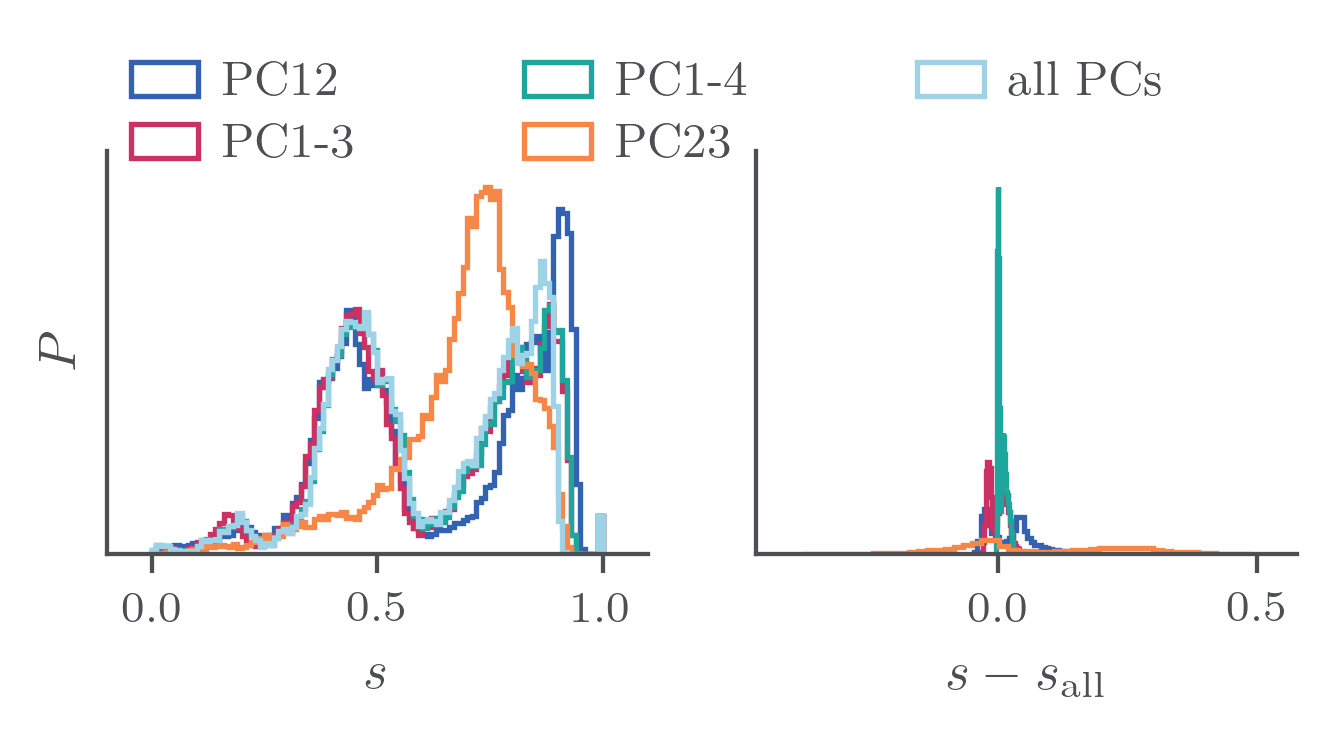
(a) St-b subset A (pulling vectors (1, 1, 0) and (1, -1, 0))

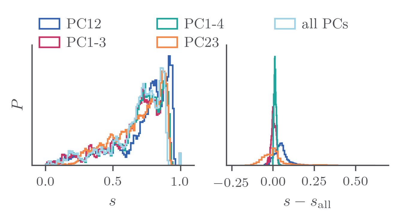
(b) St-b subset B (pulling vectors (1, 0, 1) and (1, -1, 0))

Figure S1: Left: probability distribution of the similarities calculated using different PCs. Right: probability distribution of the element-wise differences between similarities calculated based on PC subsets (e.g. PC12, PC1-3 etc.) and the full PCA space (all PCs).

First, for all sets, the RMSD and conPCA-based similarity matrices $(s_{ij})$ were calculated. For the latter, we tested principal components 1+2, 2+3, 1-3 and 1-4 and identified PCs 1-4 as a suitable subspace which contains most of the relevant information. The absolute difference between the similarities obtained from the full space and the ones from PCs 1-4 is $<0.1$, as Fig. S1 displays.

We proceeded with the determination of a suitable resolution factor $\gamma$. We tested values between $0.4$ and $0.9$. Comparing the clustering results in Figs. 1 C, D, S2 and S3  we find that a $\gamma\approx\text{median}(s_{ij})$ recovers the ground truth, i.e., the subsets of $A$ and $B$, best. This is reflected in homogeneity scores of $h=0.98$ for set $A$ and $h=0.62$ for set $B$ when using PCs 1-4, and $h=1$ for set $A$ and $h=0.92$ for set $B$ using RMSD based input features. In general, lower resolution parameters $\gamma$, here $\gamma<\text{median}(s_{ij})$, result in significant mixing of clusters in sets $B$ and $C$. Using a higher $\gamma$ enforces more homogeneous clusters and thus the identification of various smaller clusters in all investigated sets.

We therefore recommend using $\gamma=\text{median}(s_{ij})$ as starting point for pathway identification. However, it is important to note that this reasoning may be affected by the fact that our benchmark sets $A$ and $B$ are composed of only two subsets. This is reflected in set $C$, where a higher $\gamma$, between the median and the third quartile of $(s_{ij})$, yields the best clustering results.

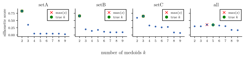
Figure S6: Silhouette scores of different St-b subsets clustered using a RMSD based similarity matrix with k-medoids. The subset is indicated in the subplot title. The red cross marks the maximal Silhouette score, while the green dot marks the true number of clusters.

Exploring k-medoids clustering as an alternative approach, Figs. 1 C, D, S4 and S5 show that this method outperforms the Leiden community detection for all three investigated sets. This follows from the design of k-medoids, as it requires the a priori definition of the number of medoids, and therefore clusters, to be known. An appropriate number of clusters can be estimated, e.g., via the Silhouette score. Figs. S6, S7 display such an analysis for all three sets and both similarity measures employed: for the benchmark sets $A$ and $B$, the Silhouette score is indeed maximal for the number of pulling directions within the sets $A$ and $B$, but not for set $C$ when using conPCA-based similarities.

In summary, k-medoids clustering demonstrates superior performance over Leiden community detection in our benchmark set. However, its effectiveness is contingent on knowing $k$, necessitating caution in scenarios beyond our benchmark system. For Leiden clustering, $\gamma=\text{median}(s_{ij})$ is a good starting point for pathway identification. In contrast to k-medoids clustering, outlier trajectories are separated without needing a user to know how many outliers there are. Clusters based on conPCA and this resolution parameter are more numerous and smaller than the those based on RMSD, but eigenvectors provide insights into the impact of specific residues on ligand pathways and thus offer valuable information on the underlying microscopic mechanisms³³.

4.2 A_2a ligand unbinding

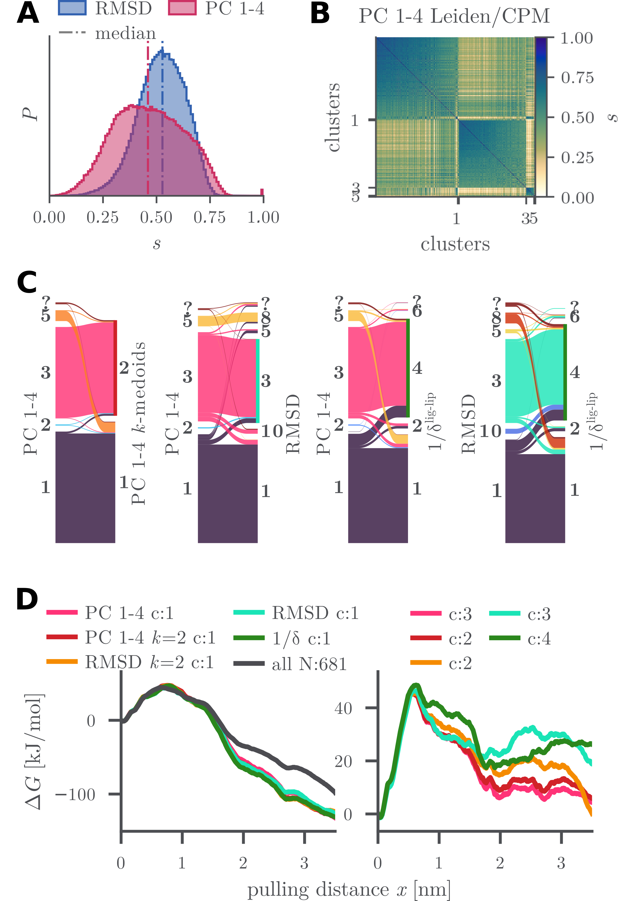
Figure 2: Trajectory clustering for pathway identification in A_2a. A: RMSD and conPCA based similarity distribution. B: Block diagonalized similarity matrix based on PCs 1-4 at $\gamma=0.46$ (equal to $\text{median}(s_{ij})$). C: Sankey plots compare the cluster contents of clustering results based on the input features PCs 1-4, RMSD and inverse ligand-lipid minimal distances $1/\delta^{\text{lig-lip}}$. Clusters with $N<3$ are combined into a single macro-cluster labeled with “?”. D: comparison of estimated free energies $\Delta G_{k}$ of clusters containing $N>100$ trajectories using the input features PC 1-4, RMSD and $1/\delta^{\text{lig-lip}}$. “c” indicates cluster number, “k” indicates the number of medoids (if applicable). The line color signifies the input feature type and clustering method. Left: clusters with $\Delta G_{k}<$-10\text{\,}\mathrm{k}\mathrm{J}\mathrm{/}\mathrm{m}\mathrm{o}\mathrm{l}$$. Right: clusters that solve the friction overestimation.

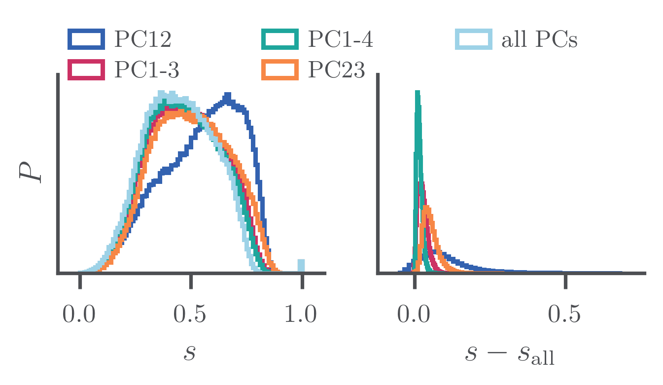
Figure S8: Left: distributions of the similarities $s$ calculated using different PCs. Right: distributions of the difference between similarities $s$ calculated in a subspace and the ones for the full PCA space $s_{\mathrm{all}}$.

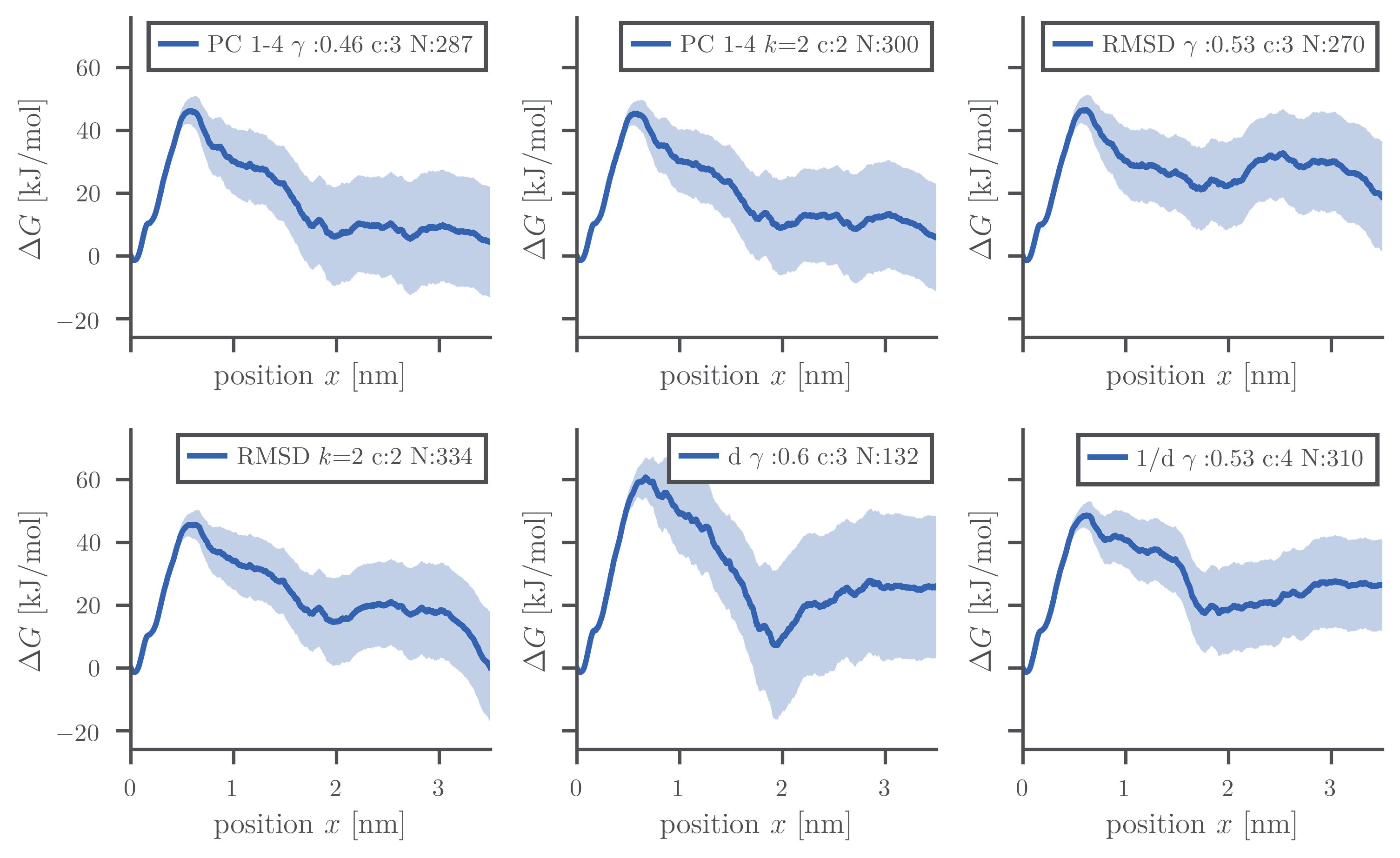
Figure S9: summary of the dcTMD results from the friction overestimation mitigating clusters. The label indicates the input feature (PC 1-4, RMSD, $\delta_{\rm ligand-lipid}$ and $1/\delta_{\rm ligand-lipid}$). In the legends, $\gamma$ denotes the used resolution parameters for Leiden/CPM based clustering and $k$ denotes the number of medoids for $k$-medoids clustering. $N$ indicates the number of trajectories in the cluster. The shaded area represents the standard deviation of 5000 bootstrapping resamples.

Following our benchmark with St-b, we applied our workflow to a more challenging protein-ligand complex, a thermostabilized variant of the A_2a receptor bound to the antagonist ZM241385.⁴⁶ We find again that the first four PCs contain the significant amount of similarities to perform trajectory clustering by consulting the similarity distributions in Fig. S8. On the basis of the the good clustering results in our benchmark system, we utilized $\gamma\approx\text{median}(s_{ij})$. The resulting similarity block matrices in Figs. 2 B and S10 show two major clusters each. Performing dcTMD analysis as displayed in Fig. 2 D and Fig. S9 shows that in each of the similarity block matrices only one cluster exhibits a mitigated friction overestimation. The other clusters exhibit artificially low free energies, due to a remaining non-normal work distribution, hinting at additional hidden CVs that we cannot resolve with our input features. As Fig. 2 C indicates, both RMSD and conPCA similarities result in comparable separations with negligible crossing within the Sankey plots. Consequently, as can be seen in Fig. 2 D, they both result in free energy curves with a barrier height of $\Delta G^{\neq}\approx 45\,$kJ/mol. The free energy in the unbound state is $\approx 5\,$kJ/mol for PCs 1-4-based clusters and $\approx 25\,$kJ/mol for RMSD clusters.

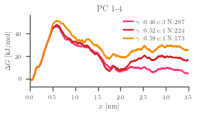
(a)

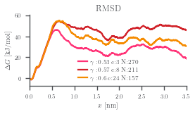
(b)

(c)

Figure S10: Estimated free energy of different PC1-4 based (a) and RMSD-based (b) Leiden/CPM clustering results. (c) RMSD-based diagonalized similarity matrix.

To assess the robustness of the predicted path-wise free energies, we tested the impact of a resolution factors $\gamma$, up to the third quartile of $(s_{ij})$, on the clustering results of both input features. Fig. S10 displays the resulting free energy estimate: with the third quartile, the number of trajectories contained in a cluster declines drastically (by about 40%). Despite this, the barriers $\Delta G^{\neq}$ show only a moderate increase of $\approx 5$-$10\,\text{kJ}/\text{mol}$. In the unbound state, however, the free energies increase to $\approx 25\,$kJ/mol for conPCA-based clusters and up to $\approx 50\,$kJ/mol for RMSD clusters.

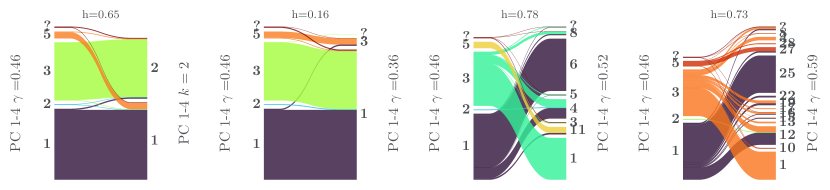
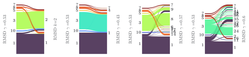
Figure S11: Sankey plots comparing contacs PCs 1-4 based (top) and RMSD-based (bottom) Leiden/CPM clustering results using $\gamma\approx\text{median}(s_{ij})$ with results of k-medoids and various $\gamma$.

This observation matches the bootstrapping errors for the Leiden clustering results using $\gamma\approx\text{median}(s_{ij})$ (see Fig. S9). While the error associated with the barrier is negligible, it reaches up to $\pm\,$20\text{\,}\mathrm{k}\mathrm{J}\mathrm{/}\mathrm{m}\mathrm{o}\mathrm{l}$$ in the unbound state. A closer analysis of the cluster composition for increasing $\gamma$ shows, comparable to the results for St-b, that the main clusters are mostly split into subclusters, yet, there is no significant mixing (see Fig. S11).

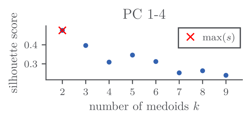
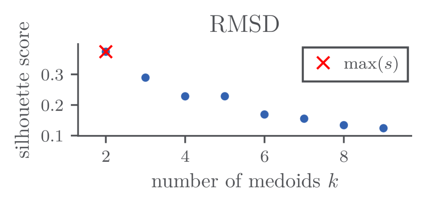
Figure S12: Silhouette scores of A_2a $k$-medoids clustering results using a contact PCs 1-4 based similarity matrix (left) and an RMSD-based similarity matrix (right). The red cross marks the maximal silhouette score.

In order to evaluate the capabilities of Leiden/CPM clustering, we compare it with other possible clustering methods, namely Leiden/Modularity⁷⁹, complete linkage ⁸⁰, $k$-medoids, and NeighborNet⁸¹, as used by us before²². The results of these tests are presented in Figs. S12 to S17. They show that the former two approaches are outperformed by Leiden/CPM, whereas $k$-medoids performs comparably. NeighborNet spreads the satisfactory RMSD cluster from Leiden/CPM across several clusters.

In summary, Leiden/CPM proves to be a well-performing trajectory clustering tool with minimal user input which mitigates the friction overestimation artefact, and results in reasonably robust free energy barriers for different values of $\gamma$. The main remaining issue is that this mitigation is only given for a single trajectory cluster. In general, finding the origin of the occurrence of pathways is limited by the chosen input features. With the information gained by identifying clusters, we reconsider our system in search for a better input feature and thus an improved RC candidate.

Exploring microscopic pathway origins

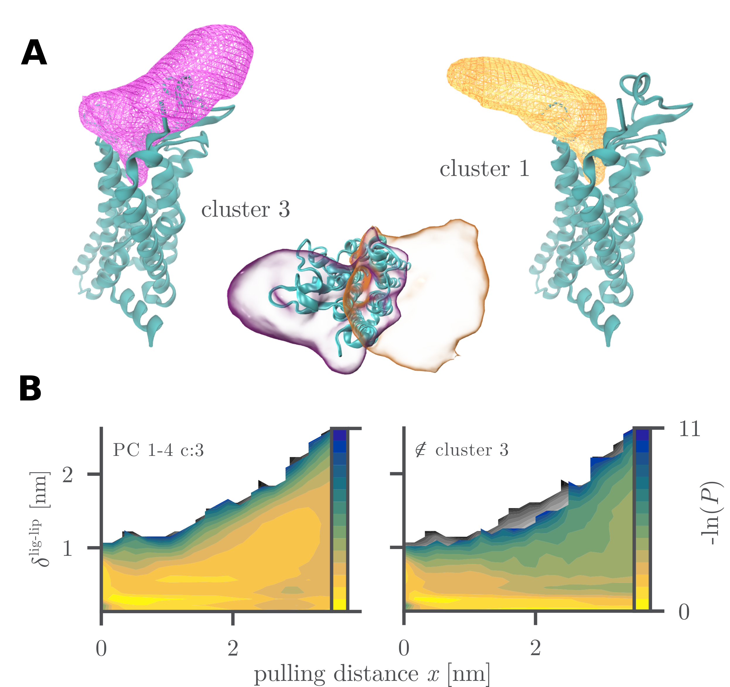
Figure 3: A: volume accessed by ZM241385 in clusters 1 and 3, respectively, based on PCs 1-4 as displayed in Fig. 2. B: probability distribution of the ligand-lipid minimal distance $\delta^{\text{lig-lip}}$ over the pulling distance $x$ of all trajectories in grayscale, overlaid by the distribution of cluster 3 (left) and its complement (right) in color.

To gain a better microscopic understanding of the ligand’s unbinding path, we visualized the volume accessed by the trajectories contained in the two main conPCA clusters 1 and 3 from Fig. 2, of which cluster 3 resolved the friction overestimation artifact. As Fig. 3 shows, this cluster moves along the extracellular loop 2 (EL2) of the receptor, whereas cluster 1 passes through the cleft between transmembrane helices 1 and 7. Since this latter route takes the ligand close to the membrane lipids, ZM241385-lipid contacts may influence the emergence of pathways. Indeed, considering the pulling distance resolved distributions of the minimal ligand-lipid distances $\delta^{\text{lig-lip}}(x)$ in Fig. 3, we find that ligands in cluster 3 move away from the membrane after a pulling distance of $\approx 1\,$nm, whereas ligands that do not belong to cluster 3 become bound to the membrane. This observation is in line with a rather high predicted hydrophobicity index for ZM241385 ($\log{P}=2.93$).⁸²

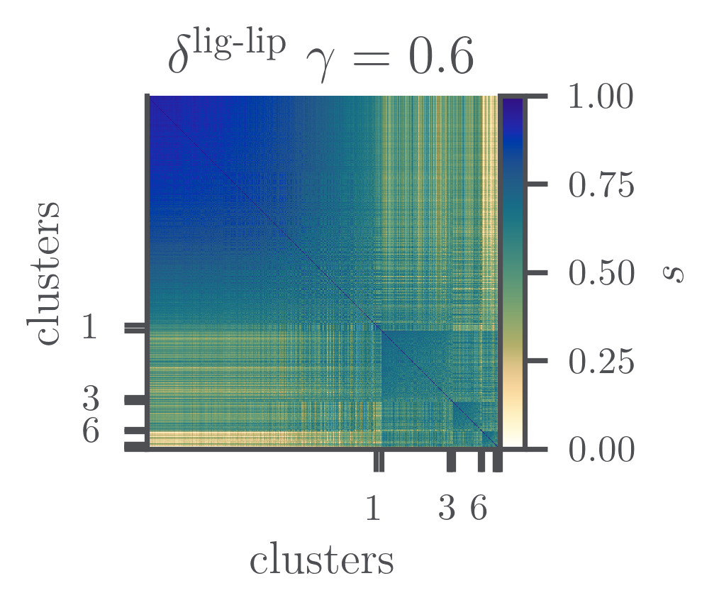
(a)

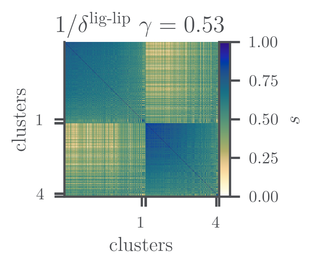
(b)

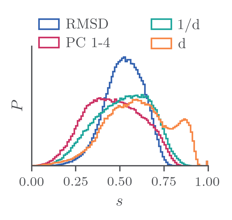
(c)

Figure S19: (a)-(b) Diagonalized similarity matrix clustering lipid-ligand minimal distances and inverse lipid-ligand minimal distances with $\gamma=\text{median}$. (c) Comparing similarity distributions of RMSD, conPCA, ligand lipid distance and inverse ligand lipid distance based similarity measures.

The characterization of friction overestimation resolving clusters in both RMSD- and conPCA-based clustering becomes more evident when plotting inverse minimal distances $1/\delta^{\text{lig-lip}}$ as shown in Fig. S19. This inspired the use of inverse ligand-lipid distance time traces $1/\delta^{\text{lig-lip}}_{i}(t)$ as input features.

We repeat our clustering approach using Leiden. Figs. 2 D, E and S14 show cluster compositions and free energy profiles comparable to the ones gained from RMSD or conPCA. Thus, we assume that the friction overestimation of cluster 1 comes from ligands entering the membrane at random times and being pushed through the water-membrane interface. We have shown earlier that dcTMD is not suited for such clusters with random switching between different regimes of dynamics.³⁴

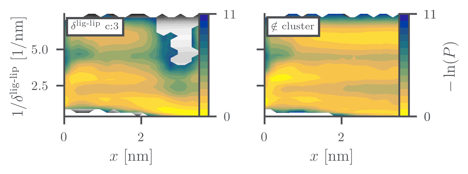
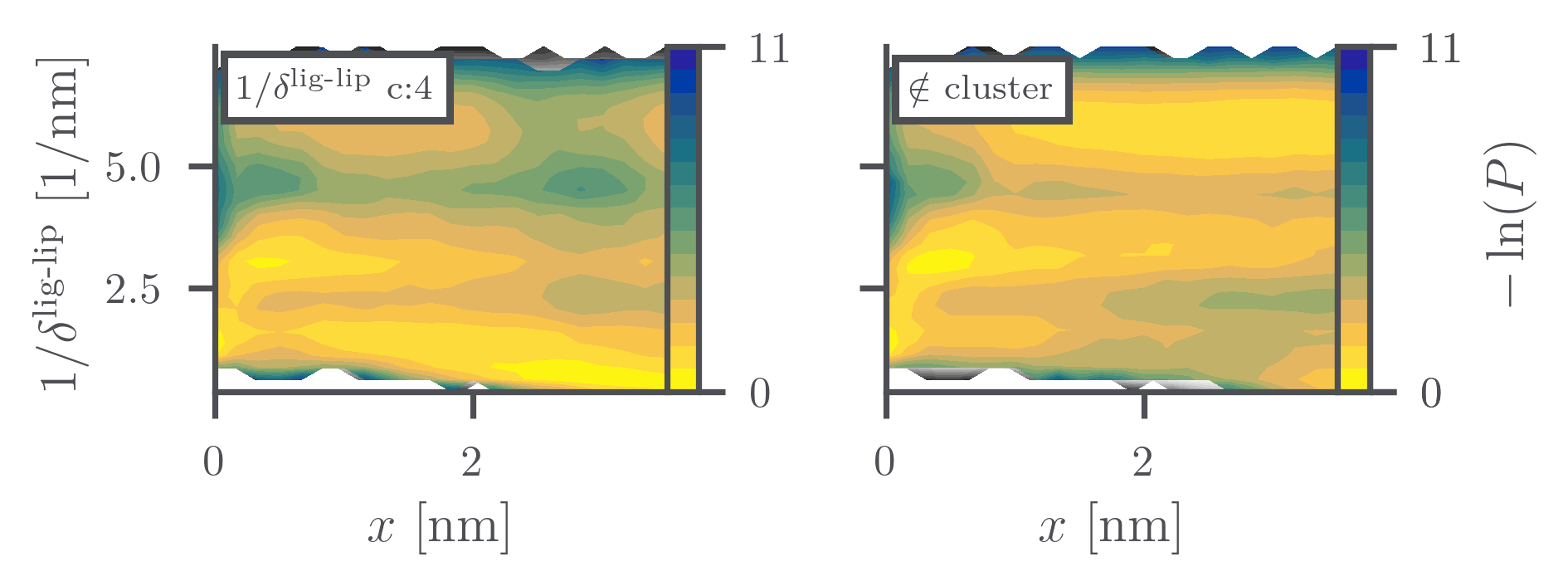
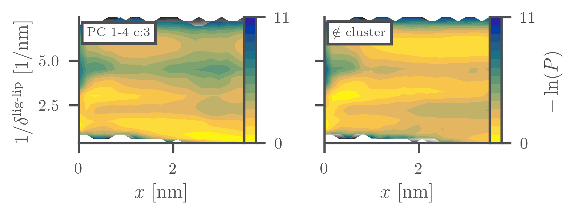
Figure S20: Inverse ligand lipid distance $1/\delta^{\text{lig-lip}}$ distribution over the pulling distance $x$ of all trajectories in grayscale, overlaid by different clustering results using $\gamma=\text{median}$ on the left and their compliment on the right. The input feature and the cluster is indicated by the label.

Focusing on the unbinding trajectory clusters from the point of view of A_2a-ligand contacts, the route of cluster 3 moves along EL2, with which the ligands form contacts (see Fig. S20). This unbinding path is in good agreement with the ZM241385 unbinding behavior described in other studies.^{83, 84} Additionally, it has been observed for the $\beta_{2}$ adrenergic receptor that EL2 forms a temporary ligand position for ligand desolvatisation,⁸⁵ which may be the case here as well, though we do not see an accompanying minimum in our free energy profiles of A2_a.

5 Conclusions

In this study, we have introduced a straightforward, easily applicable and customizable machine learning approach for the identification of unbinding pathways from a set of biased protein-ligand dissociation trajectories. Built on community detection, the method only requires the definition of a suitable similarity measure. In our benachmark RMSD-based similarities slightly outperform their conPCA-based counterparts, while for the more challenging A_2a adenosine receptor with inhibitor ZM241385 they perform similarly well. Our community detection approach succeeds in finding a relevant pathway, for which we present estimated free energy profiles. On top of that, conPCA-based similarities hold the potential to offer insight into the microscopic dynamics and lead the way towards meaningful RC candidates. Iteratively applied, the input feature space is reduced from many contact distances to four PCs and finally one distance between the ligand and the lipid bilayer as meaningful RC.

We note that while the predicted free energy barriers are robust, free energy estimates of the unbound state still vary strongly. In upcoming studies, we will investigate under which conditions the estimated profiles can be used for the prediction of unbinding and binding kinetics via Langevin equation simulations³³ in comparison to experimentally determined kinetics.

While our approach has been tailored to the needs of finding pathways in sets of trajectories with a constant velocity constraint, finding pathways in dynamical data is a far more general topic³⁷ with different approaches needing different distance measures. Biased unbinding simulations employing steered MD or infrequent metadynamics require a similarity measure taking into account unbinding events at different times. Noteworthy here is a recent study that employs dynamic time warping³⁸ as a distance measure. Our classification learning via Leiden/CPM as implemented in MoSAIC is flexible to work with any such similarity feature available.

6 Data and software availability

The dcTMD analysis tool as well as the Leiden clustering tool MoSAIC are available at https://www.moldyn.uni-freiburg.de/software.html. St-b and A_2a-ZM241385 unbinding trajectories are available from the authors upon reasonable request.

This work has been supported by the Deutsche Forschungsgemeinschaft (DFG) via grant WO 2410/2-1 within the framework of the Research Unit FOR 5099 “Reducing complexity of nonequilibrium” (project No. 431945604), the High Performance and Cloud Computing Group at the Zentrum für Datenverarbeitung of the University of Tübingen, the state of Baden-Württemberg through bwHPC and the DFG through grant no INST 37/935-1 FUGG (RV bw16I016). The authors are grateful to Gerhard Stock, Georg Diez, Fabian Koch, Daniel Nagel, Matthias Post, and Anja Seegebrecht (all University of Freiburg) for helpful discussions.

Supporting Information

Silhouette score

The Silhouette score allows to evaluate the quality of a clustering depending on the used input parameters such as the number of k-medoids or the resolution factor $\gamma$. In our case, the score is calculated per trajectory $i$. First, the mean distance $a_{i}$ in the cluster of $i$ denoted as $c_{I}$ is defined as

$$a_{i} =\frac{1}{\left|c_{I}\right|-1}\sum_{c_{I}\ni j\neq i}d(i,j)$$ (11)

where $$\left|c_{I}\right| I a_{i}$$ is the number of trajectories in the cluster . The smaller is, the better the trajectory fits in its cluster. Then, the mean distance to the neighboring cluster is defined via

$$b_{i} =\min_{J\neq I}\frac{1}{\left|c_{J}\right|}\sum_{j\in c_{J}}d(i,j),$$ (12)

which can also be expressed as the smallest mean distance to all trajectories of another cluster. The Silhouette score $$s_{i}$$ is then written as

$$s_{i} =\begin{cases}\frac{b_{i}-a_{i}}{\max\left\{a_{i},b_{i}\right\}}&\text{if $\left|c_{I}\right|>0$}\\ 0&\text{if $\left|c_{I}\right|=0$}\end{cases}$$ (13)

The mean Silhouette score $S=\left<s_{i}\right>_{i}$ can then be used to assess the quality of the clusters. An optimal $S$ is close to $1$, the worst possible value is $-1$. A maximum of the $S$ therefore suggest an optimal parameter choice.

Homogeneity score

Clustering results are compared based on homogeneity scores¹

$$h=\begin{cases}1&\text{if }H(G,K)=0\\ 1-\frac{H(G|K)}{H(G)}&\text{else}\end{cases}$$ (14)

where a data set with $N$ data points (in our case trajectories) is assumed with a set of ground truth classes $G=\{g_{i}|i=1,...,n\}$ with $n\leq N$ and a set of clusters $K=\{k_{i}|1,\dots,m\}$ with $m\leq N$. $H(G|K)$ is the conditional Shannon entropy of the class distribution given the proposed clustering, which is normalized by the maximum reduction in entropy through the clustering entropy $H(G)$, and $H(G,K)$ is the respective joint entropy. In our application, the maximal $h=1$ is given if all found clusters $K$ each only contain trajectories from one ground truth trajectory set $G$, while mixed attributions lower $h$.

Importance of the PCs for conPCA similarities: St-b

Clustering on St-b

Similarity distributions

RMSD

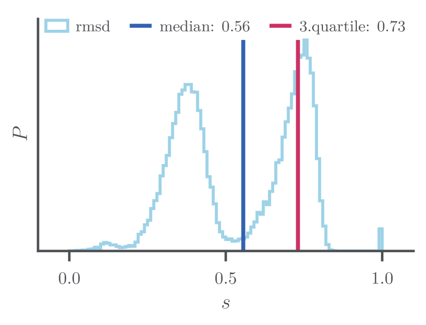
(a) set A

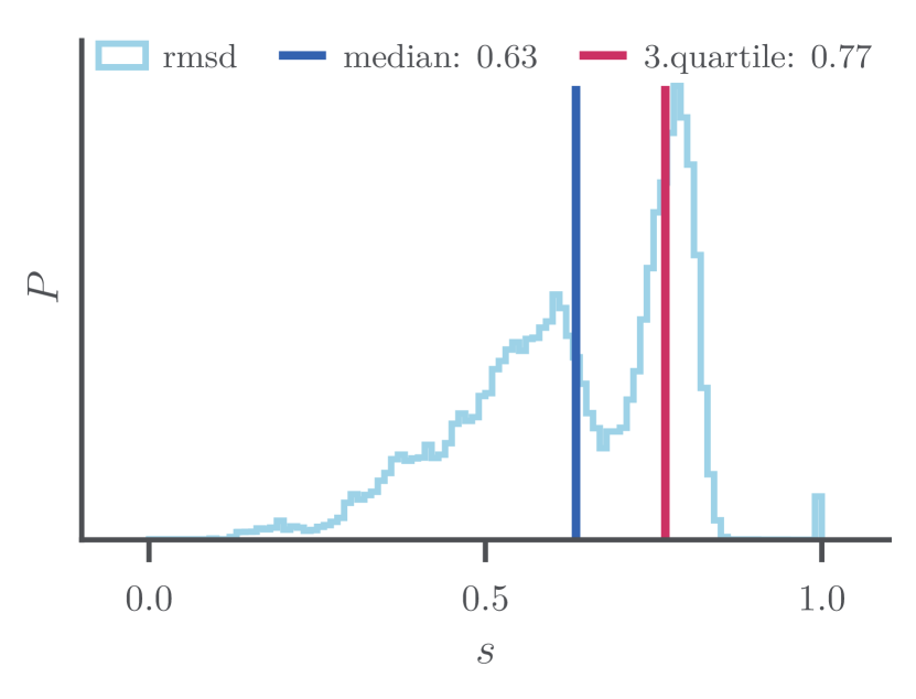
(b) set B

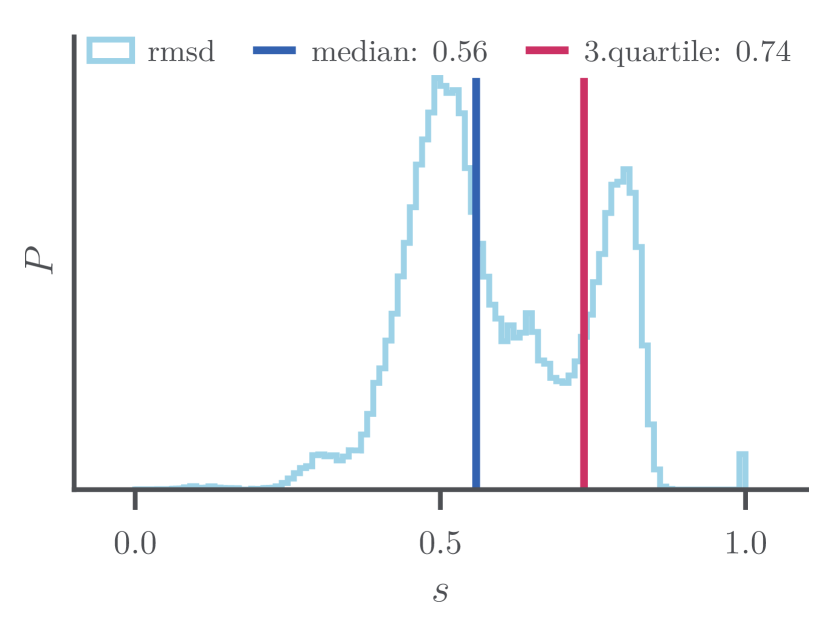
(c) set C

Figure S2: Similarity distribution for RMSD-based similarity measure. The blue line indicates the median and the red line the third quartile of the distribution.

conPCA

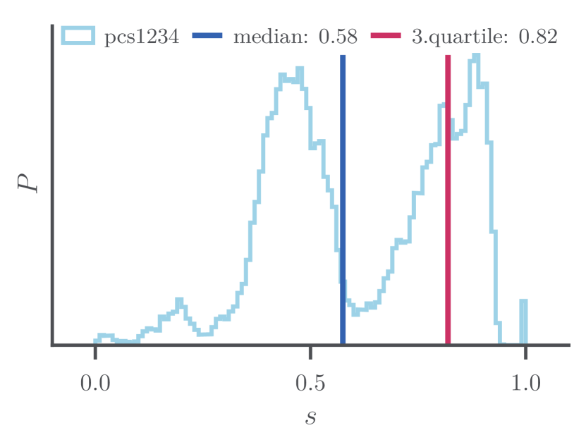
(a) set A

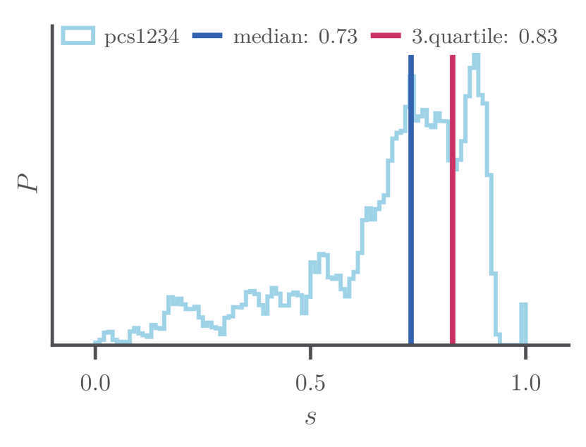
(b) set B

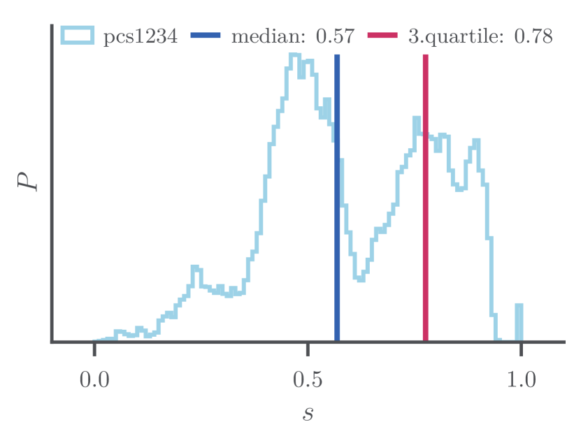
(c) set C

Figure S3: Similarity distribution for contact PCA-based similarity measure. The blue line indicates the median and the red line the third quartile of the distribution.

Clustering results: Leiden/CPM and k-medoids

RMSD

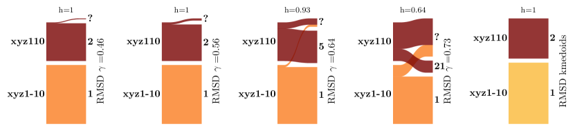
(a) set A

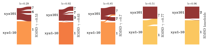
(b) set B

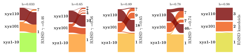
(c) set C

Figure S4: Sankey plots comparing RMSD clustering results for (a) set A, (b) set B and (c) set C. On the left of each Sankey plot, the pulling vectors are shown. The $h$ on top shows the homogeneity score, the label on the right defines the input feature (RMSD) as well as the clustering method, $\gamma$ indicating Leiden/CPM clustering.

conPCA

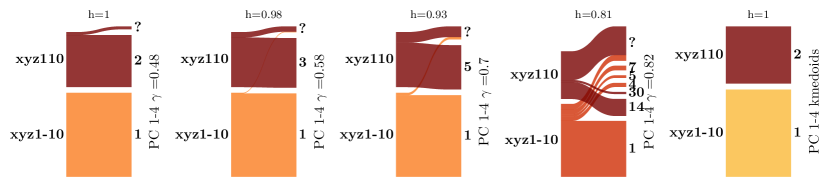
(a) set A

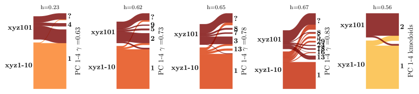
(b) set B

(c) set C

Figure S5: Sankey plots comparing RMSD clustering results for (a) set A, (b) set B and (c) set C. On the left of each Sankey plot, the pulling vectors are shown. The $h$ on top shows the homogeneity score, the label on the right defines the input feature (conPCA 1-4) as well as the clustering method, $\gamma$ indicating Leiden/CPM clustering.

k-medoids silhouette scores

RMSD

conPCA

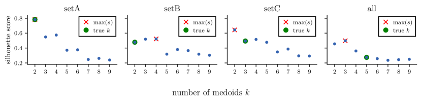
Figure S7: Silhouette scores of different St-b subsets clustered using a contact PC 1-4 based similarity matrix with k-medoids. The subset is indicated in the subplot title. The red cross marks the maximal Silhouette score, while the green dot marks the true number of clusters.

A_2a adenosine receptor

Importance of the PCs for conPCA similarities

Free energy estimation with bootstrapping errors

Clustering results: Leiden/CPM

Clustering results: k-medoids

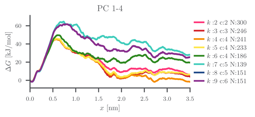
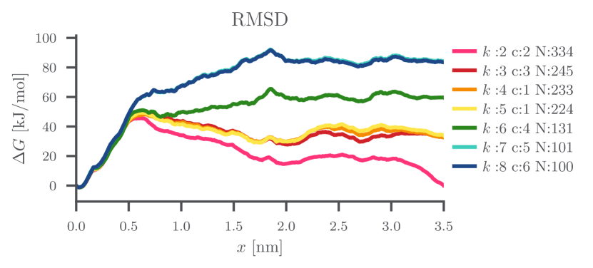
Figure S13: Estimated free energies $\Delta G$ for A_2a $k$-medoids clusters, contact PC 1-4 based (top) and RMSD based (bottom).

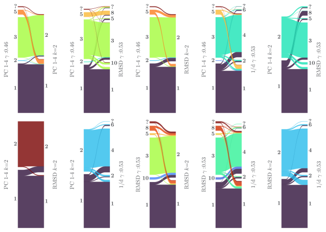
Figure S14: Sankey plots comparing RMSD Leiden clustering using CPM and k-medoids results. The Leiden/CPM results serve as comparison.

Benchmarking of additional clustering methods in A2A

The following analyses were conducted on a reduced dataset with 344 trajectories. The comparisons to Leiden/CPM clusters are thus for illustrative purposes only. These clusters are not the same as the ones in the main text, but hold the same interpretation, just for the smaller dataset.

Leiden/Modularity

The Constant Potts Model is one possible objective function for the Leiden community detection algorithm. An alternative is Modularity, which is defined as⁴²

$$\phi_{\text{mod}}=\frac{1}{2m}\sum_{c}\left(e_{c}-\frac{k_{c}^{2}}{2m}\right)$$ (15)

where we sum over all clusters $c$, the sum of similarities in a cluster is $e_{c}$, $k_{c}$ counts the similarities, i.e., graph edges, in cluster $c$ and $m$ denotes the total number of edges in the graph. Notably, this formulation of Modularity does not feature any tunable parameter that would play a similar role as $\gamma$ for the Constant Potts Model.

The similarity matrix in Fig. 15(a) reveals seven clusters, some of which have high inter-cluster similarities. Especially clusters 1 and 2 lead to the suspicion that there should be fewer clusters than suggested by the modularity objective function. The estimated free energies of all clusters of size $N>50$ are shown in Fig. 15(b). Cluster 2 seems promising and can be lumped with cluster 3 without any major impact. However, even the lumped cluster is comparatively small. Other amalgamations do not yield improved results with regard to friction overestimation. Overall, our results agree with the literature^{42, 2} that Modularity performs worse in comparison to the Constant Potts Model.

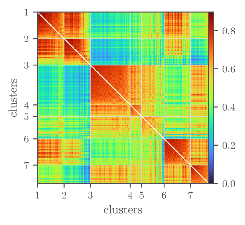
(a)

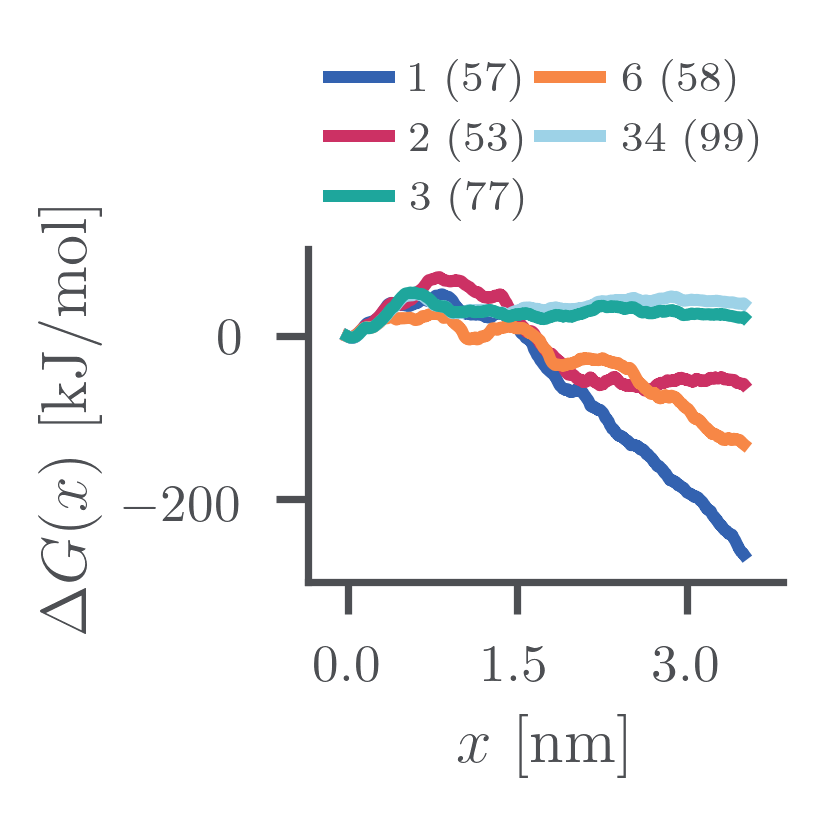
(b)

Figure S15: Results from Leiden/modularity. (a) Block-diagonalized similarity matrix. (b) Estimated free energies for the clusters with size $N>50$. The cluster $34$ is lumped from 3 and 4. The number of trajectories in a cluster is in parentheses.

Complete linkage

Next, the hierarchical method complete linkage is evaluated. A truncated dendrogram is shown in Fig. 16(a). Figure S16 b-d show the block-diagonalized similarity matrices for different values of the cutoff parameter $\gamma_{\mathrm{cl}}$ around the similarities where the splits in the dendrogram appear. Lower values quickly lead to many clusters with high inter-cluster similarity, which are thus not shown.

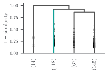
(a)

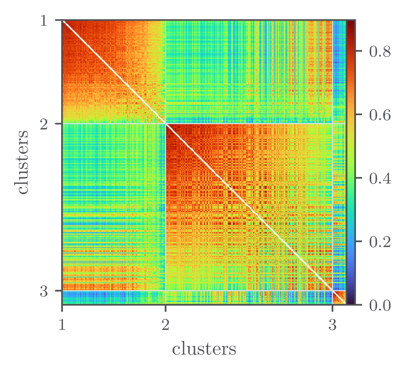
(b) $\gamma_{\mathrm{cl}}=0.92$

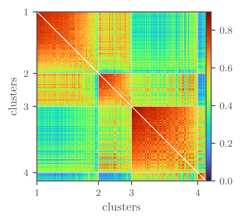
(c) $\gamma_{\mathrm{cl}}=0.85$

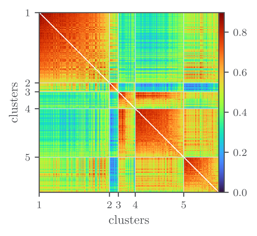
(d) $\gamma_{\mathrm{cl}}=0.70$

Figure S16: Results from complete linkage. (a) truncated dendrogram. (b)-(d) block-diagonalized similarity matrices for different resolution parameters $\gamma_{\mathrm{cl}}$.

A cluster without friction overestimation artefact, in the following denoted as ”satisfactory” cluster, first appears for $\gamma_{\mathrm{cl}}=0.92$. It is marked in green in Fig. 16(a). This cluster 1 can be found again for $\gamma_{\mathrm{cl}}=0.85$ in Fig. 16(c) as cluster 3. For $\gamma_{\mathrm{cl}}=0.70$, it is split into the clusters 3 and 4. The smaller cluster 2 can be added, which still yields a reasonable estimated free energy, as Fig. 17(a) shows. There, the satisfactory clusters from Leiden/CPM with $\gamma=0.5\text{ and }0.6$ serve as comparison. While the curves are quite similar, one of the CPM clusters is notably larger. However, with complete linkage, the shown results are the largest clusters that are reasonably possible. The Sankey plots in Fig. 17(b) and Fig. 17(c) show that the satisfactory linkage cluster $1$ is mostly preserved as cluster $12$ for Leiden/CPM with $\gamma=0.6$.

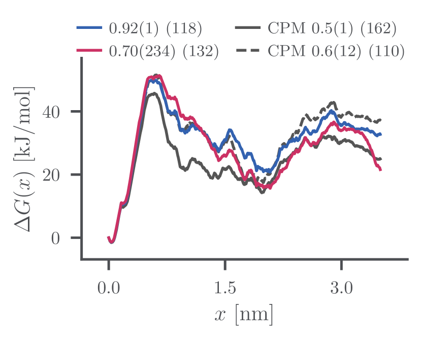
(a)

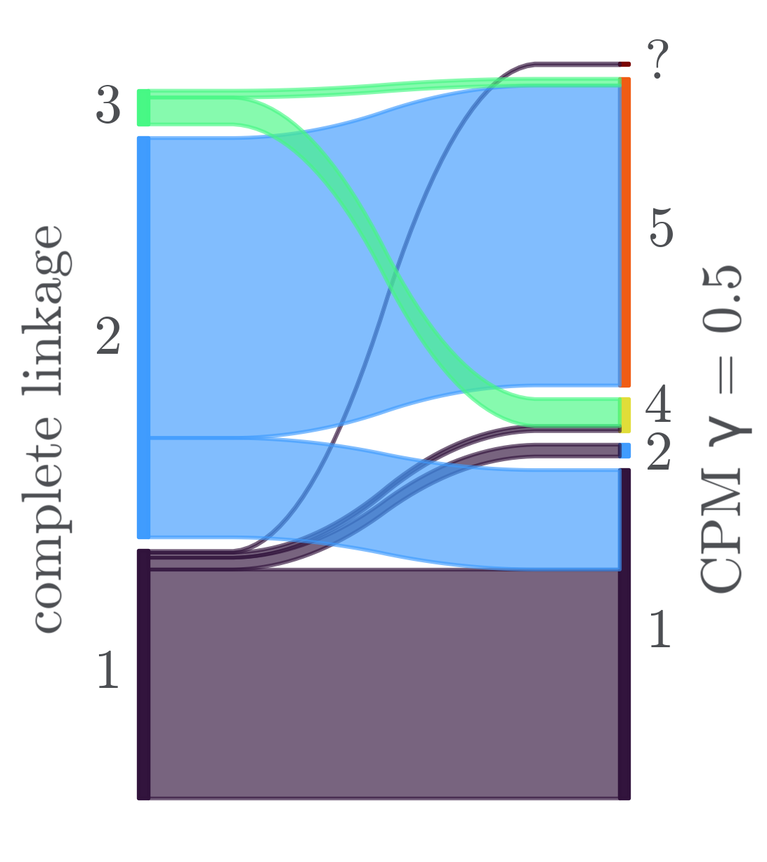
(b)

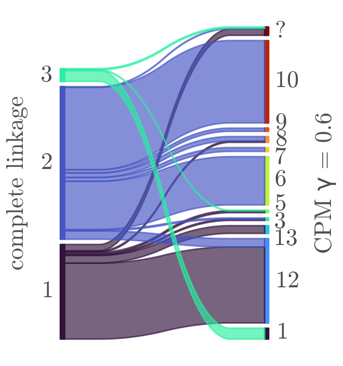
(c)

Figure S17: (a) Comparison of the estimated free energy $\Delta G$ of satisfactory clusters from complete linkage and Leiden/CPM with $\gamma=0.5$. Legend: k/$\gamma$ (cluster number(s)) (population). (b) Sankey plot between the clusters from complete linkage with $\gamma_{\mathrm{cl}}=0.92$ and Leiden/CPM with $\gamma=0.5$. (c) Sankey plot between the clusters from complete linkage with $\gamma_{\mathrm{cl}}=0.92$ and Leiden/CPM with $\gamma=0.6$. Quotation marks (“?”) bundle small clusters.

NeighborNet

The full dendrograms of linkage clustering can be difficult to assess visually. This issue is improved for the NeighborNet^{3, 4} networks, which present the entire dissimilarity matrix, and additionally take into account ambiguity in the data. This inspired a prior study from our group²², in which we recommended NeighborNet for trajectory clustering based on RMSD dissimilarities over dendrograms.

One downside of NeighborNet, however, is the need for tedious user input and comparably complex decisions, which forbids scaling the workflow. What weights even more is a second disadvantage, which we find in this study and that is visualized in Fig. S18. The NeighborNet splits graph from RMSD dissimilarities in the A_2a complex is presented, and the trajectories corresponding to a cluster from Leiden clustering similar to the ones from this study are highlighted in orange. Two points stand out: Firstly, not all nodes in the vicinity of the regions G and H are orange. Notably, the outermost trajectories denote large dissimilarities, which is why Leiden/CPM decides to exclude them from the cluster. Secondly, some isolated trajectories in the vicinity of C, D, E and F belong to the Leiden cluster as well. They often lie closely towards the cobweb-like middle of the network. This means that their distance to the cluster G or H is rather close, which is why they are more similar to G and H than the aforementioned outermost nodes. In other words, for a node, another node on the other side of the network might be closer than what appear to be its neighbors. For the pathway separation workflow, this behavior of NeighborNet is clearly undesirable.

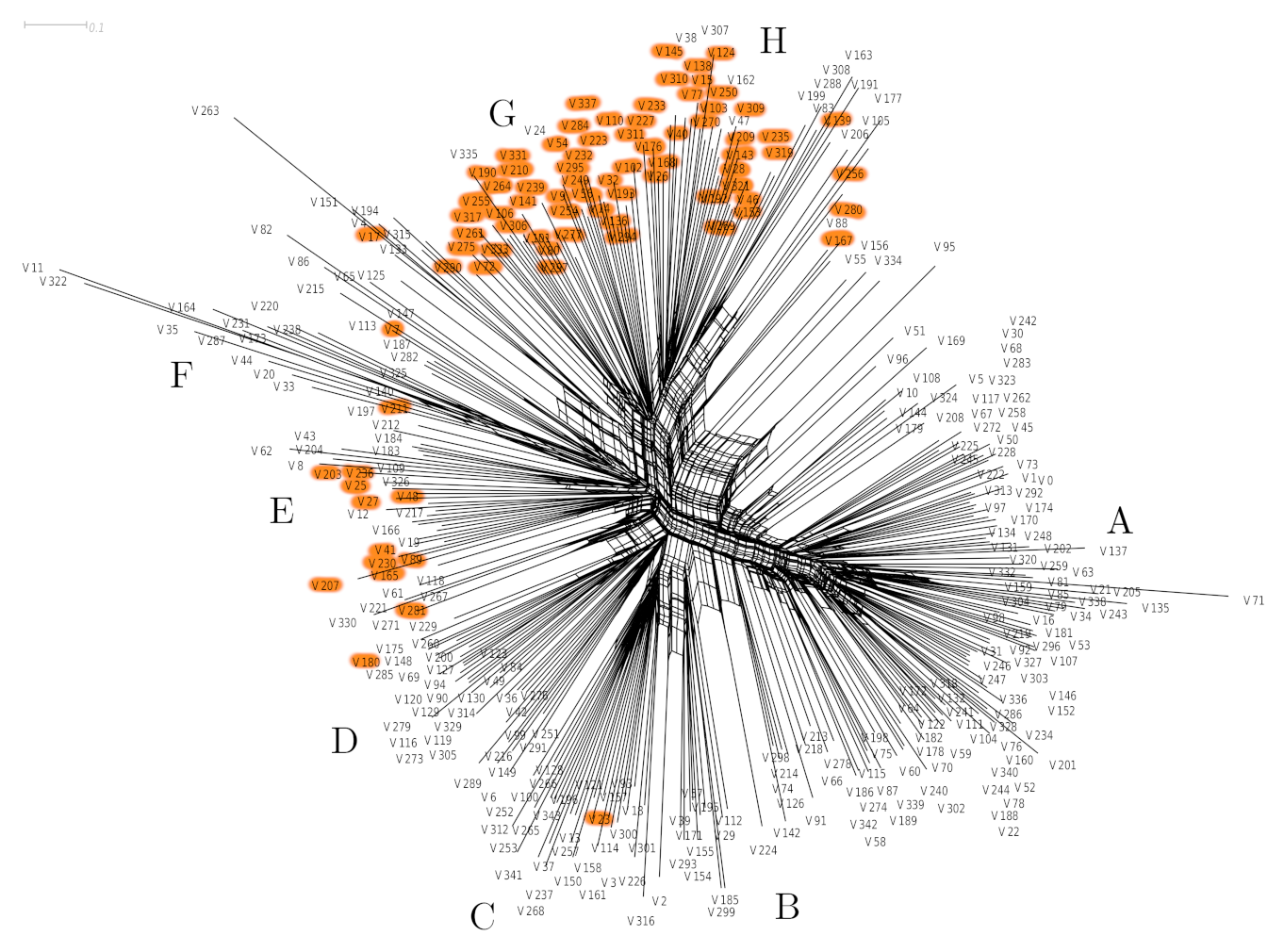
Figure S18: Comparing the RMSD NeighborNet and an RMSD Leiden/CPM for a $\gamma$ similar to the corresponding one from the main text. The trajectories from the Leiden clusters are marked in orange on the NeighborNet. The Figure was generated with SplitsTree^{huson2006application}.

A_2a ligand characteristics

Trajectory sorting via ligand lipid distances

Similarity calculation:

Euclidean distances are used to compare the ligand-lipid distance $\delta^{\text{lig-lip}}_{i}$ and inverse distance time traces $1/\delta^{\text{lig-lip}}_{i}$, respectively, of different ligand unbinding runs via

$$d^{\text{lig-lip}}_{ij} =\left<\sqrt{\left(\delta^{\text{lig-lip}}_{i}(t)-\delta^{\text{lig-lip}}_{j}(t)\right)^{2}}\right>_{t},$$

$$d^{\text{inv lig-lip}}_{ij} =\left<\sqrt{\left(1/\delta^{\text{lig-lip}}_{i}(t)-1/\delta^{\text{lig-lip}}_{j}(t)\right)^{2}}\right>_{t}.$$

To reduce it to a scalar, time-independent quantity, we average over the entire simulation time.

Ligand-extracelular loop 2 (EL2) contacts

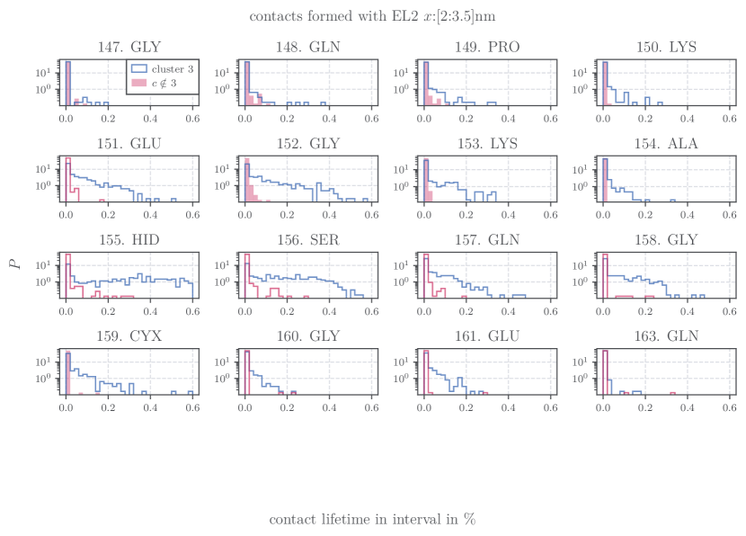
Figure S21: Comparing the population of EL2-ligand contact ($d<$3.5\text{\,}\mathrm{n}\mathrm{m}$$) lifetimes (the number of frames the contact is formed in the pulling distance interval $x:2$-$3.5\text{\,}\mathrm{n}\mathrm{m}$ in %) between cluster 4 from 1/$\delta^{\text{lig-lip}}$ $\gamma=0.53$ clustering (in blue) and its complement (in red). The solid histograms indicate a lifetime below $15\,\%$.

References

- Copeland et al. 2006 Copeland, R. A.; Pompliano, D. L.; Meek, T. D. Drug–target residence time and its implications for lead optimization. Nat. Rev. Drug Discov. 2006, 5, 730–739
- Swinney 2012 Swinney, D. C. Applications of Binding Kinetics to Drug Discovery. Pharm. Med. 2012, 22, 23–34
- Copeland 2015 Copeland, R. A. The drug–target residence time model: a 10-year retrospective. Nat. Rev. Drug Discov. 2015, 15, 87–95
- Schuetz et al. 2017 Schuetz, D. A.; de Witte, W. E. A.; Wong, Y. C.; Knasmueller, B.; Richter, L.; Kokh, D. B.; Sadiq, S. K.; Bosma, R.; Nederpelt, I.; Heitman, L. H.; Segala, E.; Amaral, M.; Guo, D.; Andres, D.; Georgi, V.; Stoddart, L. A.; Hill, S.; Cooke, R. M.; de Graaf, C.; Leurs, R.; Frech, M.; Wade, R. C.; de Lange, E. C. M.; IJzerman, A. P.; Müller-Fahrnow, A.; Ecker, G. F. Kinetics for Drug Discovery: an industry-driven effort to target drug residence time. Drug Discov. Today 2017, 22, 896–911
- Tiwary and Parrinello 2013 Tiwary, P.; Parrinello, M. From Metadynamics to Dynamics. Phys. Rev. Lett. 2013, 111, 230602
- Ray and Parrinello 2023 Ray, D.; Parrinello, M. Kinetics from Metadynamics: Principles, Applications, and Outlook. J. Chem. Theory Comput. 2023, 19, 5649–5670
- Votapka et al. 2017 Votapka, L. W.; Jagger, B. R.; Heyneman, A.; Amaro, R. E. SEEKR: simulation enabled estimation of kinetic rates, a computational tool to estimate molecular kinetics and its application to trypsin–benzamidine binding. J. Phys. Chem. B 2017, 121, 3597–3606
- Ojha et al. 2023 Ojha, A. A.; Votapka, L. W.; Amaro, R. E. QMrebind: incorporating quantum mechanical force field reparameterization at the ligand binding site for improved drug-target kinetics through milestoning simulations. Chem. Sci. 2023, 14, 13159–13175
- Kokh et al. 2018 Kokh, D. B.; Amaral, M.; Bomke, J.; Grädler, U.; Musil, D.; Buchstaller, H.-P.; Dreyer, M. K.; Frech, M.; Lowinski, M.; Vallée, F.; Bianciotto, M.; Rak, A.; Wade, R. C. Estimation of Drug-Target Residence Times by -Random Acceleration Molecular Dynamics Simulations. J. Chem. Theory Comput. 2018, 14, 3859–3869
- Miao et al. 2020 Miao, Y.; Bhattarai, A.; Wang, J. Ligand Gaussian Accelerated Molecular Dynamics (LiGaMD): Characterization of Ligand Binding Thermodynamics and Kinetics. J. Chem. Theory Comput. 2020, 16, 5526–5547
- Rico et al. 2019 Rico, F.; Russek, A.; González, L.; Grubmüller, H.; Scheuring, S. Heterogeneous and rate-dependent streptavidin–biotin unbinding revealed by high-speed force spectroscopy and atomistic simulations. Proc. Natl. Acad. Sci. USA 2019, 116, 6594–6601
- Potterton et al. 2019 Potterton, A.; Husseini, F. S.; Southey, M. W. Y.; Bodkin, M. J.; Heifetz, A.; Coveney, P. V.; Townsend-Nicholson, A. Ensemble-Based Steered Molecular Dynamics Predicts Relative Residence Time of A 2AReceptor Binders. J. Chem. Theory Comput. 2019, 15, 3316–3330
- Cai et al. 2023 Cai, W.; Jäger, M.; Bullerjahn, J. T.; Hugel, T.; Wolf, S.; Balzer, B. N. Anisotropic Friction in a Ligand-Protein Complex. Nano Lett. 2023, 23, 4111–4119
- Iida and Kameda 2023 Iida, S.; Kameda, T. Dissociation Rate Calculation via Constant-Force Steered Molecular Dynamics Simulation. J. Chem. Inf. Model. 2023, 63, 3369–3376
- Wolf 2023 Wolf, S. Predicting Protein-Ligand Binding and Unbinding Kinetics with Biased MD Simulations and Coarse-Graining of Dynamics: Current State and Challenges. J. Chem. Inf. Model. 2023, 63, 2902–2910
- Tiwary et al. 2015 Tiwary, P.; Limongelli, V.; Salvalaglio, M.; Parrinello, M. Kinetics of protein–ligand unbinding: Predicting pathways, rates, and rate-limiting steps. Proc. Natl. Acad. Sci. USA 2015, 112, E386–E391
- Schuetz et al. 2019 Schuetz, D. A.; Bernetti, M.; Bertazzo, M.; Musil, D.; Eggenweiler, H.-M.; Recanatini, M.; Masetti, M.; Ecker, G. F.; Cavalli, A. Predicting Residence Time and Drug Unbinding Pathway through Scaled Molecular Dynamics. J. Chem. Inf. Model. 2019, 59, 535–549
- Capelli et al. 2019 Capelli, R.; Carloni, P.; Parrinello, M. Exhaustive Search of Ligand Binding Pathways via Volume-Based Metadynamics. J. Phys. Chem. Lett. 2019, 3495–3499
- Rydzewski and Valsson 2019 Rydzewski, J.; Valsson, O. Finding multiple reaction pathways of ligand unbinding. J. Chem. Phys. 2019, 150, 221101
- Kokh et al. 2020 Kokh, D. B.; Doser, B.; Richter, S.; Ormersbach, F.; Cheng, X.; Wade, R. C. A workflow for exploring ligand dissociation from a macromolecule: Efficient random acceleration molecular dynamics simulation and interaction fingerprint analysis of ligand trajectories. J. Chem. Phys. 2020, 153, 125102
- Bianciotto et al. 2021 Bianciotto, M.; Gkeka, P.; Kokh, D. B.; Wade, R. C.; Minoux, H. Contact Map Fingerprints of Protein-Ligand Unbinding Trajectories Reveal Mechanisms Determining Residence Times Computed from Scaled Molecular Dynamics. J. Chem. Theory Comput. 2021, 17, 6522–6535
- Bray et al. 2022 Bray, S.; Tänzel, V.; Wolf, S. Ligand Unbinding Pathway and Mechanism Analysis Assisted by Machine Learning and Graph Methods. J. Chem. Inf. Model. 2022, 62, 4591–4604
- Motta et al. 2022 Motta, S.; Callea, L.; Bonati, L.; Bonati; Pandini, A. PathDetect-SOM: A neural network approach for the identification of pathways in ligand binding simulations. J. Chem. Theory Comput. 2022, 18, 1957–1968
- Ribeiro et al. 2020 Ribeiro, J. M. L.; Provasi, D.; Filizola, M. A combination of machine learning and infrequent metadynamics to efficiently predict kinetic rates, transition states, and molecular determinants of drug dissociation from G protein-coupled receptors. J. Chem. Phys. 2020, 153, 124105
- Bertazzo et al. 2021 Bertazzo, M.; Gobbo, D.; Decherchi, S.; Cavalli, A. Machine Learning and Enhanced Sampling Simulations for Computing the Potential of Mean Force and Standard Binding Free Energy. J. Chem. Theory Comput. 2021, 17, 5287–5300
- Badaoui et al. 2022 Badaoui, M.; Buigues, P. J.; Berta, D.; Mandana, G. M.; Gu, H.; Földes, T.; Dickson, C. J.; Hornak, V.; Kato, M.; Molteni, C.; Parsons, S.; Rosta, E. Combined Free-Energy Calculation and Machine Learning Methods for Understanding Ligand Unbinding Kinetics. J. Chem. Theory Comput. 2022, 18, 2543–2555
- France-Lanord et al. 2023 France-Lanord, A.; Vroylandt, H.; Salanne, M.; Rotenberg, B.; Saitta, A. M.; Pietrucci, F. Data-driven path collective variables. arxiv 2023, 2312.13868
- Fröhlking et al. 2024 Fröhlking, T.; Bonati, L.; Rizzi, V.; Gervasio, F. L. Deep learning path-like collective variable for enhanced sampling molecular dynamics. arxiv 2024, 2402.01508
- Wolf and Stock 2018 Wolf, S.; Stock, G. Targeted molecular dynamics calculations of free energy profiles using a nonequilibrium friction correction. J. Chem. Theory Comput. 2018, 14, 6175––6182
- Post et al. 2023 Post, M.; Wolf, S.; Stock, G. Investigation of Rare Protein Conformational Transitions via Dissipation-Corrected Targeted Molecular Dynamics. J. Chem. Theory Comput. 2023, 19, 8978–8986
- Zwanzig 2001 Zwanzig, R. Nonequilibrium Statistical Mechanics; Oxford University: Oxford, 2001
- Schilling 2022 Schilling, T. Coarse-grained modelling out of equilibrium. Phys. Rep. 2022, 972, 1–45
- Wolf et al. 2020 Wolf, S.; Lickert, B.; Bray, S.; Stock, G. Multisecond ligand dissociation dynamics from atomistic simulations. Nat. Commun. 2020, 11, 2918
- Wolf et al. 2023 Wolf, S.; Post, M.; Stock, G. Path separation of dissipation-corrected targeted molecular dynamics simulations of protein–ligand unbinding. J. Chem. Phys. 2023, 158, 124106
- Bolhuis et al. 2002 Bolhuis, P. G.; Chandler, D.; Dellago, C.; Geissler, P. L. Transition path sampling: Throwing ropes over rough mountain passes, in the dark. Annu. Rev. Phys. Chem. 2002, 53, 291–318
- Berryman and Schilling 2010 Berryman, J. T.; Schilling, T. Sampling rare events in nonequilibrium and nonstationary systems. J. Chem. Phys. 2010, 133, 244101
- Yuan et al. 2017 Yuan, G.; Sun, P.; Zhao, J.; Li, D.; Wang, C. A review of moving object trajectory clustering algorithms. Artif. Intell. Rev. 2017, 47, 123–144
- Ray and Parrinello 2023 Ray, D.; Parrinello, M. Data Driven Classification of Ligand Unbinding Pathways. arxiv 2023, 2308.05752
- Sittel and Stock 2018 Sittel, F.; Stock, G. Perspective: Identification of collective variables and metastable states of protein dynamics. J. Chem. Phys. 2018, 149, 150901
- Nagel et al. 2023 Nagel, D.; Sartore, S.; Stock, G. Selecting Features for Markov Modeling: A Case Study on HP35. J. Chem. Theory Comput. 2023,
- Traag et al. 2011 Traag, V. A.; Van Dooren, P.; Nesterov, Y. Narrow scope for resolution-limit-free community detection. Phys. Rev. E 2011, 84, 016114
- Diez et al. 2022 Diez, G.; Nagel, D.; Stock, G. Correlation-Based Feature Selection to Identify Functional Dynamics in Proteins. J. Chem. Theory Comput. 2022, 18, 5079–5088
- Ernst et al. 2015 Ernst, M.; Sittel, F.; Stock, G. Contact- and distance-based principal component analysis of protein dynamics. J. Chem. Phys. 2015, 143, 244114
- Lebon et al. 2011 Lebon, G.; Warne, T.; Edwards, P. C.; Bennett, K.; Langmead, C. J.; Leslie, A. G. W.; Tate, C. G. Agonist-bound adenosine A2A receptor structures reveal common features of GPCR activation. Nature 2011, 474, 521–525
- Doré et al. 2011 Doré, A. S.; Robertson, N.; Errey, J. C.; Ng, I.; Hollenstein, K.; Tehan, B.; Hurrell, E.; Bennett, K.; Congreve, M.; Magnani, F.; Tate, C. G.; Weir, M.; Marshall, F. H. Structure of the adenosine A(2A) receptor in complex with ZM241385 and the xanthines XAC and caffeine. Structure 2011, 19, 1283–1293
- Segala et al. 2016 Segala, E.; Guo, D.; Cheng, R. K. Y.; Bortolato, A.; Deflorian, F.; Doré, A. S.; Errey, J. C.; Heitman, L. H.; IJzerman, A. P.; Marshall, F. H.; Cooke, R. M. Controlling the Dissociation of Ligands from the Adenosine A2A Receptor through Modulation of Salt Bridge Strength. J. Med. Chem. 2016, 59, 6470–6479
- Schlitter et al. 1994 Schlitter, J.; Engels, M.; Krüger, P. Targeted Molecular Dynamics - A New Approach for Searching Pathways of Conformational Transitions. J. Mol. Graph. 1994, 12, 84–89
- Jarzynski 1997 Jarzynski, C. Nonequilibrium equality for free energy differences. Phys. Rev. Lett. 1997, 78, 2690–2693
- Park and Schulten 2004 Park, S.; Schulten, K. Calculating potentials of mean force from steered molecular dynamics simulations. J. Chem. Phys. 2004, 120, 5946–5961
- Jäger et al. 2021 Jäger, M.; Koslowski, T.; Wolf, S. Predicting Ion Channel Conductance via Dissipation-Corrected Targeted Molecular Dynamics and Langevin Equation Simulations. J. Chem. Theory Comput. 2021, 18, 494–502
- Jackson 1991 Jackson, J. E. A user’s guide to principal components; John Wiley & Sons, 1991
- Post et al. 2019 Post, M.; Wolf, S.; Stock, G. Principal component analysis of nonequilibrium molecular dynamics simulations. J. Chem. Phys. 2019, 150, 204110
- Traag et al. 2019 Traag, V. A.; Waltman, L.; van Eck, N. J. From Louvain to Leiden: guaranteeing well-connected communities. Sci. Rep. 2019, 9, 5233
- Le Trong et al. 2011 Le Trong, I.; Wang, Z.; Hyre, D. E.; Lybrand, T. P.; Stayton, P. S.; Stenkamp, R. E.; IUCr Streptavidin and its biotin complex at atomic resolution. Act. Crystallogr. D 2011, 67, 813–821
- Hornak et al. 2006 Hornak, V.; Abel, R.; Okur, A.; Strockbine, B.; Roitberg, A.; Simmerling, C. Comparison of multiple Amber force fields and development of improved protein backbone parameters. Proteins 2006, 65, 712–725
- Best and Hummer 2009 Best, R. B.; Hummer, G. Optimized Molecular Dynamics Force Fields Applied to the Helix-Coil Transition of Polypeptides. J. Phys. Chem. B 2009, 113, 9004–9015
- Lindorff-Larsen et al. 2010 Lindorff-Larsen, K.; Piana, S.; Palmo, K.; Maragakis, P.; Klepeis, J. L.; Dror, R. O.; Shaw, D. E. Improved side-chain torsion potentials for the Amber ff99SB protein force field. Proteins 2010, 78, 1950–1958
- Jorgensen et al. 1983 Jorgensen, W. L.; Chandrasekhar, J.; Madura, J. D.; Impey, R. W.; Klein, M. Comparison of simple potential functions for simulating liquid water. J. Chem. Phys. 1983, 79, 926
- Wang and Brüschweiler 2006 Wang, J.; Brüschweiler, R. 2D Entropy of Discrete Molecular Ensembles. J. Chem. Theory Comput. 2006, 2, 18–24
- Sousa da Silva and Vranken 2012 Sousa da Silva, A. W.; Vranken, W. F. ACPYPE - AnteChamber PYthon Parser interfacE. BMC Res. Notes 2012, 5, 367
- Wang et al. 2004 Wang, J. M.; Wolf, R. M.; Caldwell, J. W.; Kollman, P. A.; Case, D. A. Development and testing of a general amber force field. J. Comput. Chem. 2004, 25, 1157–1174
- Neese 2012 Neese, F. The ORCA program system. WIREs Comput. Mol. Sci. 2012, 2, 73–78
- Lu and Chen 2012 Lu, T.; Chen, F. Multiwfn: A multifunctional wavefunction analyzer. J. Comput. Chem. 2012, 33, 580–592
- Abraham et al. 2015 Abraham, M. J.; Murtola, T.; Schulz, R.; Pall, S.; Smith, J. C.; Hess, B.; Lindahl, E. GROMACS: High performance molecular simulations through multi-level parallelism from laptops to supercomputers. SoftwareX 2015, 1, 19–25
- Waterhouse et al. 2018 Waterhouse, A.; Bertoni, M.; Bienert, S.; Studer, G.; Tauriello, G.; Gumienny, R.; Heer, F. T.; de Beer, T. A. P.; Rempfer, C.; Bordoli, L.; Lepore, R.; Schwede, T. SWISS-MODEL: homology modelling of protein structures and complexes. Nucl. Acids Res. 2018, 46, W296–W303
- Olsson et al. 2011 Olsson, M. H.; Søndergaard, C. R.; Rostkowski, M.; Jensen, J. H. PROPKA3: consistent treatment of internal and surface residues in empirical p K a predictions. J. Chem. Theory Comput. 2011, 7, 525–537
- Berger et al. 1997 Berger, O.; Edholm, O.; Jähnig, F. Molecular dynamics simulations of a fluid bilayer of dipalmitoylphosphatidylcholine at full hydration, constant pressure, and constant temperature. Biophys. J. 1997, 72, 2002–2013
- Schmidt and Kandt 2012 Schmidt, T. H.; Kandt, C. LAMBADA and InflateGRO2: efficient membrane alignment and insertion of membrane proteins for molecular dynamics simulations. J. Chem. Inf. Model. 2012, 52, 2657–2669
- Cordomí et al. 2012 Cordomí, A.; Caltabiano, G.; Pardo, L. Membrane Protein Simulations Using AMBER Force Field and Berger Lipid Parameters. J. Chem. Theory Comput. 2012, 8, 948–958
- Tieleman et al. 1999 Tieleman, D. P.; Sansom, M. S.; berendsen, H. J. Alamethicin helices in a bilayer and in solution: molecular dynamics simulations. Biophys. J. 1999, 76, 40–49
- Wolf et al. 2008 Wolf, S.; Böckmann, M.; Höweler, U.; Schlitter, J.; Gerwert, K. Simulations of a G protein-coupled receptor homology model predict dynamic features and a ligand binding site. FEBS Lett. 2008, 582, 3335–3342
- Bussi and Parrinello 2007 Bussi, G.; Parrinello, M. Accurate sampling using Langevin dynamics. Phys. Rev. E 2007, 75, 056707
- Parrinello and Rahman 1981 Parrinello, M.; Rahman, A. Polymorphic transitions in single crystals: A new molecular dynamics method. J. Appl. Phys. 1981, 52, 7182–7190
- Madhulatha 2012 Madhulatha, T. S. An Overview of Clustering Methods. IOSR J. Eng. 2012, 02, 719–725
- Rosenberg and Hirschberg 2007 Rosenberg, A.; Hirschberg, J. V-Measure: A Conditional Entropy-Based External Cluster Evaluation Measure. Proceedings of the 2007 Joint Conference on Empirical Methods in Natural Language Processing and Computational Natural Language Learning (EMNLP-CoNLL). Prague, Czech Republic, 2007; pp 410–420
- Gowers et al. 2016 Gowers, R. J.; Linke, M.; Barnoud, J.; Reddy, T. J.; Melo, M. N.; Seyler, S. L.; Domanski, J.; Dotson, D. L.; Buchoux, S.; Kenney, I. M.; others MDAnalysis: a Python package for the rapid analysis of molecular dynamics simulations. Proceedings of the 15th python in science conference. 2016; p 105
- Golob 2018 Golob, A. pySankey. 2018; \urlhttps://github.com/anazalea/pySankey
- Humphrey et al. 1996 Humphrey, W.; Dalke, A.; Schulten, K. VMD – Visual Molecular Dynamics. J. Mol. Graph. 1996, 14, 33–38
- Newman and Girvan 2004 Newman, M. E.; Girvan, M. Finding and evaluating community structure in networks. Phys. Rev. E 2004, 69, 26113
- Sørensen 1948 Sørensen, T. A Method of Establishing Groups of Equal Amplitude in Plant Sociology Based on Similarity of Species Content and Its Application to Analyses of the Vegetation on Danish Commons; Biologiske skrifter; Munksgaard in Komm., 1948; Vol. 5; pp 1–34
- Huson et al. 2010 Huson, D. H.; Rupp, R.; Scornavacca, C. Phylogenetic Networks: Concepts, Algorithms and Applications.; Cambridge University Press: Cambridge, United Kingdom, 2010
- 82 The ChEMBL database Compound ZM-241385. \urlhttps://www.ebi.ac.uk/chembl/compound/report/card/CHEMBL113142/, accessed 29.07.2022
- Mattedi et al. 2019 Mattedi, G.; Deflorian, F.; Mason, J. S.; de Graaf, C.; Gervasio, F. L. Understanding Ligand Binding Selectivity in a Prototypical GPCR Family. J. Chem. Inf. Model. 2019, 59, 2830–2836
- Deganutti et al. 2020 Deganutti, G.; Moro, S.; Reynolds, C. A. A Supervised Molecular Dynamics Approach to Unbiased Ligand–Protein Unbinding. J. Chem. Inf. Model. 2020, 60, 1804–1817
- Dror et al. 2011 Dror, R. O.; Pan, A. C.; Arlow, D. H.; Borhani, D. W.; Maragakis, P.; Shan, Y.; Xu, H.; Shaw, D. E. Pathway and mechanism of drug binding to G-protein-coupled receptors. Proc. Natl. Acad. Sci. USA 2011, 108, 13118–13123

References

- Rosenberg and Hirschberg 2007 Rosenberg, A.; Hirschberg, J. V-Measure: A Conditional Entropy-Based External Cluster Evaluation Measure. Proceedings of the 2007 Joint Conference on Empirical Methods in Natural Language Processing and Computational Natural Language Learning (EMNLP-CoNLL). Prague, Czech Republic, 2007; pp 410–420
- Traag et al. 2019 Traag, V.; Waltman, L.; van Eck, N. From Louvain to Leiden: guaranteeing well-connected communities. Sci. Rep. 2019, 9, 5233
- Bryant and Moulton 2002 Bryant, D.; Moulton, V. NeighborNet: An agglomerative method for the construction of planar phylogenetic networks. Algorithms in Bioinformatics: Second International Workshop, WABI 2002 Rome, Italy, September 17–21, 2002 Proceedings 2. 2002; pp 375–391
- Bryant and Moulton 2004 Bryant, D.; Moulton, V. Neighbor-net: an agglomerative method for the construction of phylogenetic networks. Mol. Biol. Evol. 2004, 21, 255–265