Shortest-path percolation on complex networks

Abstract

We propose a bond-percolation model intended to describe the consumption, and eventual exhaustion, of resources in transport networks. Edges forming minimum-length paths connecting demanded origin-destination nodes are removed if below a certain budget. As pairs of nodes are demanded and edges are removed, the macroscopic connected component of the graph disappears, i.e., the graph undergoes a percolation transition. Here, we study such a shortest-path-percolation transition in homogeneous random graphs where pairs of demanded origin-destination nodes are randomly generated, and fully characterize it by means of finite-size scaling analysis. If budget is finite, the transition is identical to the one of ordinary percolation, where a single giant cluster shrinks as edges are removed from the graph; for infinite budget, the transition becomes more abrupt than the one of ordinary percolation, being characterized by the sudden fragmentation of the giant connected component into a multitude of clusters of similar size.

Percolation theory studies the relation between the macroscopic connectedness of a system and its microscopic structure. Percolation models are fruitfully applied to many physical systems, e.g., gelation of molecules, diffusion in porous media, and forest fires [1]. In network science, percolation models are traditionally used to characterize the robustness of social, biological, and economic networks [2, 3, 4, 5, 6, 7]. The existence of a macroscopic connected component in a network is interpreted as a proxy of its overall function. The connectedness of the network may be compromised by the deletion or failure of its microscopic components, either nodes (site percolation) or edges (bond percolation). The protocol used to delete the network’s microscopic elements defines the specific percolation model at hand. In the ordinary percolation model, deleted microscopic elements are chosen uniformly at random [1]. Other well-known percolation models include targeted attacks [4], $k$-core percolation [8], cascading failures [9], explosive percolation [10], and optimal percolation [11]. These protocols can be extended to account for multiplexity [9, 12] and higher-order interactions [13].

Percolation-based approaches are popular also in the analysis of dynamical processes occurring on infrastructural networks, e.g., car congestion in road networks [14, 15, 16, 17, 18]. By assigning a quality score to each edge (i.e., road segment) and removing edges with quality below a given threshold, the above-mentioned studies focus on how the emergence of congested clusters affects the overall function of a road network. Similar approaches are used to study road networks subject to flooding [19, 20] and sidewalk networks in cities during the pandemic [21].

Here, we introduce a bond-percolation model specifically devised to mimic the utilization and progressive exhaustion of a transport network’s resources. We named it as the shortest-path-percolation (SPP) model because edges are removed from the network whenever they form paths of minimum length connecting pairs of nodes. A real system that is genuinely described by the SPP model is an airline network where travelers select minimum-cost itineraries connecting their desired origin-destination airports [22]. The utilization of any other infrastructure devoted to the transport of people, goods or information can also be well described by the SPP model.

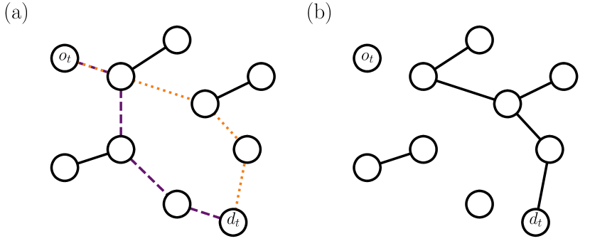
Figure 1: The shortest-path-percolation (SPP) model. (a) There are two possible shortest paths connecting the origin-destination pair $o_{t}\to d_{t}$ demanded by the agent $t$, denoted by orange dotted edges and purple dashed edges, respectively. The length of such shortest paths is $Q_{t}=4$. (b) If the maximum length allowed in the SPP model is $C\geq 4$, one of the two shortest paths is selected at random, then all of its edges are removed from the graph. Here, all purple dashed edges are deleted, and the graph fragments into four clusters.

The SPP model is defined as follows. For $t>0$, we denote with $\mathcal{G}_{t}=(\mathcal{V},\mathcal{E}_{t})$, composed of $N=|\mathcal{V}|$ nodes and $E_{t}=|\mathcal{E}_{t}|$ edges, the undirected and unweighted graph available to the agent $t$, and with $o_{t}\to d_{t}$ the origin-destination pair demanded by the agent $t$. If at least a path between $o_{t}$ and $d_{t}$ exists in $\mathcal{G}_{t}$, we denote with $Q_{t}$ the length of the shortest one(s). The demand of the agent $t$ can be supplied only if $d_{t}$ is reachable from $o_{t}$ and $Q_{t}\leq C$, where $C>0$ is a tunable parameter of the model. If one shortest path satisfying this condition is identified (one path is selected at random if more than one exists), namely $(o_{t}=i_{1},i_{2},\ldots,i_{Q_{t}+1}=d_{t})$, all edges in the path are removed from $\mathcal{G}_{t}$, i.e., $\mathcal{E}_{t}\mapsto\mathcal{E}_{t}\setminus\bigcup_{q=1}^{Q_{t}}(i_{q},i_{q+1})$, see Fig. 1. If no path exists between $o_{t}$ and $d_{t}$ or if $Q_{t}>C$, no edge is removed from the graph. In either case, we copy the graph $\mathcal{G}_{t+1}\mapsto\mathcal{G}_{t}$ and then increase $t\mapsto t+1$. The process is repeated until no more demand is requested/can be supplied.

The behaviour of the SPP model depends on the structure of the graph $\mathcal{G}_{1}$ and the demand of the agents. Here, for simplicity, we assume that the graph $\mathcal{G}_{1}$ is an instance of the Erdős-Rényi (ER) model with exactly $E_{1}=\bar{k}N/2$ edges, with $\bar{k}$ average degree of the graph. We further assume that the origin-destination nodes $o_{t}\to d_{t}$ demanded by the agent $t$ are chosen uniformly at random. These assumptions allow us to contrast results obtained for the SPP model to those of other well-studied percolation models. Specifically, for $C=1$, the SPP model effectively reduces to the ordinary bond-percolation model on ER graphs displaying a smooth transition when a fraction $p_{c}=1-1/\bar{k}$ of randomly selected edges is removed from the graph. For $C>1$, the SPP model differentiates from the ordinary bond-percolation model as edges in the graph are no longer deleted independently, rather in a correlated fashion.

We note that for $C=N$ the inequality $Q_{t}\leq C$ always holds when $o_{t}$ and $d_{t}$ are in the same connected component of the graph $\mathcal{G}_{t}$. We refer to this setting as the infinite-$C$ case as the maximal length of an allowed path is proportional to the network size (the effective infinite-budget case occurs when $C$ scales at least as $N^{\delta}$, with $\delta=0.431\pm 0.001$, see SM). If the above condition for $C$ is not satisfied, for example we choose $C=1$ for all $N$ values, then we denote it as the finite-$C$ case.

$C$	$p_{c}$	$\beta/\bar{\nu}$	$\gamma/\bar{\nu}$
$1$	$0.750\pm 0.001$	$0.301\pm 0.003$	$0.339\pm 0.003$
$2$	$0.702\pm 0.001$	$0.287\pm 0.004$	$0.351\pm 0.001$
$3$	$0.683\pm 0.001$	$0.284\pm 0.005$	$0.358\pm 0.003$
$\infty$	$0.651\pm 0.002$	$0.210\pm 0.001$	$0.545\pm 0.002$

Table 1: Critical properties of the shortest-path-percolation (SPP) model. From left to right, we report: the value of the input parameter $C$ of the SPP model, the estimate of the critical threshold $p_{c}$, the ratio of the critical exponents $\beta/\bar{\nu}$ and $\gamma/\bar{\nu}$. Estimates reported here are obtained via finite-size scaling analysis in the event-based ensemble.

We fully characterize the behaviour of the SPP model on ER graphs with a systematic numerical analysis. Our results are based on $5,000$ independent simulations of the SPP model for each combination of $N$ and $C$ values. In each realization, we first generate an ER graph with average degree $\bar{k}=4$ and then apply the SPP model to it. As for the control parameters, we focus our attention to both the fraction of removed edges $p$ as well as the raw number of demanded origin-destination pairs $t$. We determine the properties of the SPP transition via finite-size scaling (FSS) analysis relying on the conventional ensemble where sampled configurations correspond to independent realizations of the SPP model obtained at specific values of the control parameters [1]. All results hold when using the so-called event-based ensemble [23, 24]. To construct this ensemble, we still sample one configuration from each individual realization of the SPP model; such a sampled configuration is the one corresponding to the largest change, caused by the deletion of a single edge, in the size of the largest cluster during the SPP process.

Our main finding is that SPP belongs to the same universality class as of ordinary percolation as long as $C$ is finite; for infinite $C$, the SPP transition becomes more abrupt than ordinary percolation, being characterized by a set of different critical exponents, see Table 1 and SM.

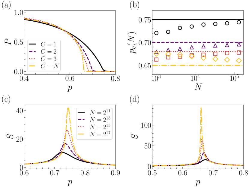
Figure 2: Shortest-path percolation transition in the conventional ensemble. (a) Percolation strength $P$ as a function of fraction of removed edges $p$ with different values of $C$. The SPP model is applied to Erdős-Rényi (ER) graphs with size $N=2^{17}$ (b) Pseudo-critical point $p_{c}(N)$ as a function of $N$ for different values of $C$. The horizontal line denotes the estimated critical point $p_{c}$ for each $C$. (c) Average cluster size $S$ as a function of $p$ for ER graphs for different network sizes $N$. Here $C=1$. (d) Similar to (b) but for $C=N$.

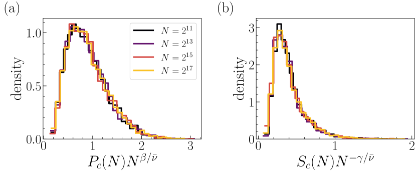
Figure 3: Shortest-path-percolation transition in the event-based ensemble. Here we used $C=\infty$. (a) The distribution of ${P}_{c}(N)\,N^{\beta/\bar{\nu}}$ with $\beta/\bar{\nu}=0.210$. Different curves correspond to different network sizes $N$. (b) Same as in (a) but for $S_{c}(N)\,N^{-\gamma/\bar{\nu}}$ with $\gamma/\bar{\nu}=0.545$.

In Fig. 2, we report results valid under the conventional ensemble. In Fig. 2 (a), we plot the percolation strength $P$ as a function of $p$. We fix the network size to $N=2^{17}$ and compare results obtained for different $C$ values. We observe that, as $C$ increases, the change displayed by $P$ becomes more abrupt. The different behaviours of the finite- vs. infinite-$C$ cases are apparent by looking at how the average cluster size $S$ changes as a function of $p$, see Figs. 2 (c) and (d), with $S$ being characterized by a peak value $S_{c}(N)$ occurring at the pseudo-critical point $p_{c}(N)$. We observe that $S_{c}(N)\sim N^{\gamma/\bar{\nu}}$, with $\gamma/\bar{\nu}=0.333\pm 0.002$ if $C=1$ and $\gamma/\bar{\nu}=0.528\pm 0.002$ for $C=\infty$ (see SM). Also, we find that $p_{c}=p_{c}(N)+bN^{-1/\bar{\nu}}$ for any $C$ value, see Fig. 2 (b). Not surprisingly, the value of the critical point $p_{c}$ is a decreasing function of $C$, ranging from $p_{c}=0.750\pm 0.001$ for $C=1$ to $p_{c}=0.650\pm 0.001$ for $C=\infty$; however, we surprisingly find that $b>0$ and $1/\bar{\nu}\simeq 1/3$ for finite $C$, but $b<0$ and $1/\bar{\nu}=0.23\pm 0.01$ for infinite $C$. The observed difference in the value of the critical exponent $\bar{\nu}$ as well as the change of the sign of the fitting parameter $b$ denote that a fundamentally different type of percolation transition takes place depending on whether $C$ is finite or infinite.

In Fig. 3, we display results for the FSS analysis under the event-based ensemble. Specifically, we display the collapse of the distributions of the rescaled pseudo-critical observables $P_{c}(N)\,N^{\beta/\bar{\nu}}$ and $S_{c}(N)\,N^{-\gamma/\bar{\nu}}$. Both plots appearing in Fig. 3 refer to the infinite-$C$ case; we report results valid for finite $C$ in the SM. We find $\beta/\bar{\nu}=0.210\pm 0.001$ and $\gamma/\bar{\nu}=0.545\pm 0.002$ for $C=\infty$. Comparable values of the ratio $\beta/\bar{\nu}$ are obtained by monitoring the scaling of the peak values of the $k$-th largest clusters, for $k=2,3,4,$ and $5$ (see SM). Note that these estimates are compatible with the known hyperscaling relation $2\beta/\bar{\nu}+\gamma/\bar{\nu}=1$. For finite $C$, we recover $\beta/\bar{\nu}\simeq\gamma/\bar{\nu}\simeq 1/\bar{\nu}\simeq 1/3$ for both the ensembles, as expected for ordinary percolation [1] (see SM). The critical exponent ratios $\beta/\bar{\nu}$ and $\gamma/\bar{\nu}$ obtained via FSS at the pseudo-critical point $p_{c}(N)$ in the conventional ensemble are compatible with those valid for the event-based ensemble; at the critical point $p_{c}$, the estimates are different, likely because affected by finite-size effects (SM).

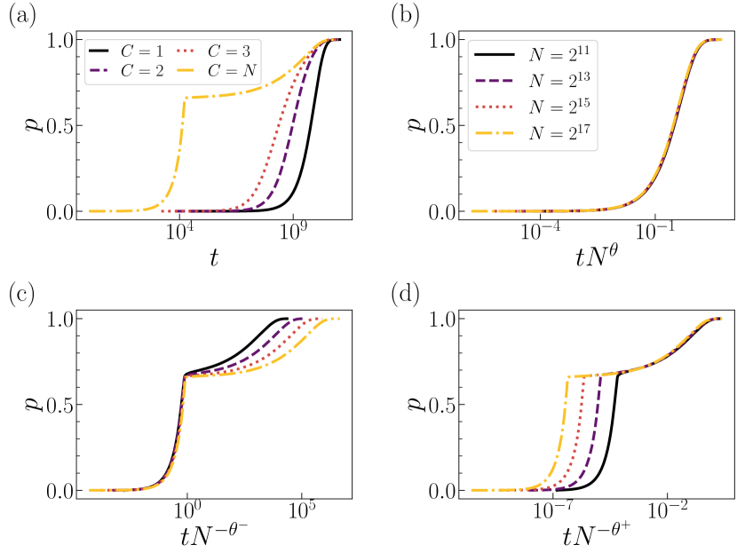
Figure 4: Control parameters in the shortest-path percolation model. (a) The fraction of removed edges $p$ is plotted as a function of number of demanding agents $t$ for different values of $C$. Results are valid for Erdős-Rényi graphs with size $N=2^{17}$. (b) Same as in (a), but for for $C=1$ and different $N$ values. The abscissas values are rescaled as $tN^{-\theta}$, with $\theta=2.014$, to obtain a collapse between the various curves. (c) Same as in (b), but for $C=N$. The collapse is obtained by rescaling the abscissas as $tN^{-\theta^{-}}$, with $\theta^{-}=0.843$. (d) Same as in (c), but rescaling the abscissas as $tN^{-\theta^{+}}$, with $\theta^{+}=2.068$.

The study of the standard observables of Fig. 2 and Fig. 3 highlights a marked difference between the finite- and infinite-$C$ transitions, however, does not convey an actual physical explanation of such a finding. A clear picture emerges from the analysis of Fig. 4, where we study the mapping between the two natural control parameters of the SPP model, i.e., $p$ and $t$. For finite $C$, $p$ and $t$ are mapped one to the other by a universal smooth function that is revealed by rescaling $t\mapsto tN^{-\theta}$. We estimate $\theta=2.014\pm 0.002$ for $C=1$, see Fig. 4 (b) and SM, and similar values for other finite-$C$ cases (see SM). The scaling exponent $\theta\simeq 2$ tells us that the dismantling of the network requires to select a number of origin-destination pairs that is proportional to the total number of node pairs in the network. When $C$ is infinite, however, two distinct universal behaviors are visible: (i) for $t\leq t_{c}(N)$, curve collapse is obtained by plotting $p$ vs. $tN^{-\theta^{-}}$ with $\theta^{-}=0.843\pm 0.004$; (ii) for $t>t_{c}(N)$, data collapse is obtained by rescaling $t\mapsto tN^{-\theta^{+}}$ with $\theta^{+}=2.068\pm 0.004$. Note that the kink point $t_{c}(N)$ is such that $p(t_{c}(N))=p_{c}(N)$. The finding can be interpreted as follows. When the giant cluster is present, edges are removed with ease as a path exists between most pairs of nodes. At the beginning, the number of removed edges per pair is small as the shortest-path length between pairs of randomly selected nodes is short. However, as the graph becomes sparser, the average shortest-path length increases, so does the number of edges removed per demanded pair. Critical behaviour corresponds to the consumption of a large number of edges for a small number of demanded pairs. In particular, the number of pairs that needs to be demanded to reach the critical point is a vanishing fraction of the total number of pairs of nodes in the network, as the value of the scaling exponent $\theta^{-}$ indicates. After such a massive consumption of edges, the network is fragmented into multiple clusters. In this configuration, two randomly selected nodes are unlikely to belong to the same connected component. This leads to a dramatic slow down in the number of edges removed per pair of demanded origin-destination nodes. Also, individual clusters have a finite diameter, thus each of them is dismantled by an effectively finite-$C$ SPP process, hence $\theta^{+}\simeq 2$.

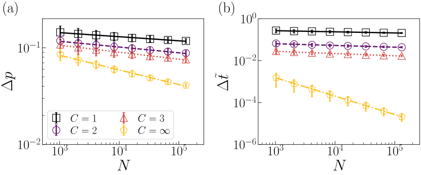
Figure 5: Abruptness of the shortest-path-percolation transition. (a) We plot $\Delta p$ vs. $N$ for different $C$ values. We represent the average value of $\Delta p$ with symbols; the size of the error bars is proportional to its standard deviation. Displayed lines represent the best fits of the scaling $\Delta p\sim N^{-\alpha}$. We get $\alpha=0.042\pm 0.001$ for $C=1$, $\alpha=0.059\pm 0.002$ for $C=2$, $\alpha=0.072\pm 0.003$ for $C=3$, and $\alpha=0.151\pm 0.004$ for $C=\infty$. (b) $\Delta\tilde{t}$ vs. $N$. Lines stand for best fits of the scaling $\Delta\tilde{t}\sim N^{-\alpha^{\prime}}$. We find $\alpha^{\prime}=0.053\pm 0.002$ for $C=1$, $\alpha^{\prime}=0.083\pm 0.004$ for $C=2$, $\alpha^{\prime}=0.106\pm 0.005$ for $C=3$, and $\alpha^{\prime}=0.878\pm 0.004$ for $C=\infty$.

We assess the abruptness of the SPP transition using the same procedure as in Refs. [10, 25], and measure the width of the transition window as $\Delta p=p_{2}-p_{1}$ or $\Delta\tilde{t}=(t_{2}-t_{1})\,N^{-2}$, where $p_{2}$ and $t_{2}$ are the highest values of the control parameters for which $P>0.5$, whereas $p_{1}$ and $t_{1}$ are the highest values of the control parameters for which $P>1/\sqrt{N}$. The width of the transition in terms of origin-destination pairs of nodes is further normalized. As the results of Fig. 5 show, we find that $\Delta p\sim N^{-\alpha}$. The value of the scaling exponent is almost zero for finite $C$, e.g., $\alpha=0.042\pm 0.001$ for $C=1$, denoting that the transition is continuous; for $C=\infty$, we find $\alpha=0.151\pm 0.004$, meaning that the transition is weekly discontinuous [25]. In the latter case, the exponent value is smaller than the one observed for the explosive percolation transition, thus indicating a less abrupt change of phases. The weekly discontinuous nature of the infinite-$C$ SPP transition becomes very apparent by looking at the scaling $\Delta\tilde{t}\sim N^{-\alpha^{\prime}}$, where we find $\alpha^{\prime}=0.878\pm 0.004$. We find instead $\alpha^{\prime}\simeq 0$ for finite $C$, e.g., $\alpha^{\prime}=0.053\pm 0.002$ for $C=1$, once more denoting a continuous transition.

To sum up, we introduce the shortest-path-percolation (SPP) model aimed at mimicking the utilization, and eventual exhaustion, of a network’s resources by agents demanding minimum-cost itineraries below a certain budget. The main finding of our systematic analysis about the application of the SPP model to Erdős-Rényi graphs is that, if budget is finite, then exhaustion occurs similarly as in an ordinary percolation process; however, if budget is unbounded, then the network’s resources are consumed abruptly, in a similar fashion as for the of explosive percolation model [10]. The abruptness of the SPP transition, however, is not the result of a competitive selection criterion that takes advantage of knowledge about the cluster structure of the graph as in the explosive percolation model [25], rather caused by topological correlations among groups of deleted edges. Our findings underscore that not only dynamical processes, but also fundamental structural transitions such as percolation are radically altered by framing them in terms of path-based rather than edge-based models [26].

The SPP model can account for arbitrary forms of demand and can be easily generalized to deal with directed, weighted, time-stamped graphs. Thus, in addition to its theoretical appeal, we believe that the model may be important for the development of computational frameworks aimed at analyzing and optimizing real-world infrastructural networks.

I Supplemental Material

II Shortest-path-percolation algorithm

The inputs of the algorithm are: (i) a graph $\mathcal{G}_{1}=(\mathcal{V},\mathcal{E}_{1})$ composed of $N=|\mathcal{V}|$ nodes and $E_{1}=|\mathcal{E}_{1}|$ edges; (ii) a list of $T$ origin-destination pairs, i.e., $(o_{1}\to d_{1},o_{2}\to d_{2},\ldots,o_{t}\to d_{t},\ldots,o_{T}\to d_{T})$; the maximum budget $C$ available to each agent. We assume that the graph $\mathcal{G}_{1}$ is unweighted and symmetric.

We denote with $\mathcal{G}_{t}=(\mathcal{V},\mathcal{E}_{t})$ the infrastructural graph available to the $t$-th agent when the agent demands an itinerary for its origin-destination $o_{t}\to d_{t}$. We set $t=1$ and iterate the following:

1. We find all shortest paths between the origin $o_{t}$ and the destination $d_{t}$; the shortest paths are found on the graph $\mathcal{G}_{t}$ using only edges in the set $\mathcal{E}_{t}$. Denote with $Q_{t}$ the length of such shortest path. We copy the graph $\mathcal{G}_{t+1}\mapsto\mathcal{G}_{t}$.

2. If there is no path from $o_{t}$ to $d_{t}$ or if $Q_{t}>C$, we proceed to point 4.

3. If a path from $o_{t}$ to $d_{t}$ exists and $Q_{t}\leq C$, then we select one of the shortest paths between $o_{t}$ and $d_{t}$ at random. We denote this path as $(i_{0}=o_{t},i_{1},i_{2},\ldots,i_{Q_{t}-1},i_{Q_{t}}=d_{t})$,. All edges in the path are removed from the current graph, i.e., $\mathcal{E}_{t+1}\mapsto\mathcal{E}_{t}\setminus\bigcup_{q=1}^{Q_{t}}(i_{q-1},i_{q})$.

4. We increase $t\mapsto t+1$ and go back to point 1.

The former algorithm is iterated until $t\leq T$.

A random shortest path between a generic pair of nodes $o$ and $d$ can be efficiently selected by first applying a breadth-first search (BFS) from $o$ to $d$. We perform a BFS with maximum depth $C$, as only shortest paths of length at most equal to $C$ are considered. If node $d$ is not reached with a BFS with maximum depth $C$ then no shortest path shorter than $C$ exists between $o$ and $d$. While performing BFS, we construct a directed acyclic graph (DAG) that contains the entire information about all eventual shortest paths between $o$ and $d$. Specifically, for a generic node $i$ in the DAG, we store the information about its parents in the set $\mathcal{P}_{i}$. Also, we keep track of the number of shortest paths $s_{i}$ that originate in node $o$ and arrive to node $i$. Once BFS is completed, we sample one of the shortest paths between $o$ and $d$ by performing a random walk from $d$ to $o$ on the DAG. At each generic node $i$ along the sampled walk, we walk back towards $o$ by randomly selecting a parent of $i$ from the set $\mathcal{P}_{i}$. The parent $j\in\mathcal{P}_{i}$ is selected proportionally to the pre-computed number of shortest paths $s_{j}$ passing thorough it.

II.1 Shortest-path percolation for randomly selected pairs of nodes

In our paper, we study the case in which the shortest-path-percolation (SPP) model assumes that a random origin-destination pair is selected at a time. The naive implementation of this procedure could be computationally inefficient as potentially many of the randomly generated pairs may not satisfy the above requirement, thus leading to a very large number of attempts before a suitable pair is effectively generated. The issue is exacerbated for finite $C$ and when the graph progressively becomes sparser/disconnected due to the removal of edges.

To avoid the computational issue and be able to simulate the model in sufficiently large networks, we proceed as follows. We first construct the set of potentially suitable origin-destination pairs, i.e., $\mathcal{L}=\{o_{1}\to d_{1},o_{2}\to d_{2},\ldots,o_{z}\to d_{z},\ldots,o_{Z}\to d_{Z}\}$, as the set of all origin-destination nodes at distance less than or equal to $C$ in the graph $\mathcal{G}_{1}$. Nodes in the network are labeled from $1$ to $N$, in the set $\mathcal{L}$ we have only pairs $o_{z}<d_{z}$ to avoid double counting. We set $t=1$, and then apply the following:

1. We extract a random number $\tau$ from the geometric distribution

   $$P(\tau)=\frac{2L}{N(N-1)}\,\left[1-\frac{2L}{N(N-1)}\right]^{\tau-1}\;,$$ (S1)

   where $L$ is the number of pairs in the list $\mathcal{L}$. The probability of success in the geometric distribution is $\frac{2L}{N(N-1)}$, and $\tau$ represents the number of random pairs that one needs to generate in order to find a pair that belongs to $\mathcal{L}$. We create the graph $\mathcal{G}_{t+\tau}\mapsto\mathcal{G}_{t}$. Then, we increase $t\mapsto t+\tau$.

2. We select a random pair, say $o_{t}\to d_{t}$, from the list $\mathcal{L}$. We apply the shortest-path-percolation algorithm by first determining whether $o_{t}$ and $d_{t}$ are in the same connected component and finding all eventual shortest paths connecting the two nodes. We then remove all edges along the shortest path between $o_{t}$ and $d_{t}$ only if such a shortest path exists and has length smaller or equal than $C$. Similarly to what we described in the preceding section, this step is performed on the graph $\mathcal{G}_{t}$. The result of the operation is the graph $\mathcal{G}_{t}$ containing $E_{t}$ edges.

3. We verify that the pair $o_{t}\to d_{t}$ can still belong to the list $\mathcal{L}$ by measuring the shortest-path distance between $o_{t}$ and $d_{t}$ in the graph $\mathcal{G}_{t}$. If such a distance is larger than $C$, we remove the pair $o_{t}\to d_{t}$ from $\mathcal{L}$, i.e., $\mathcal{L}\mapsto\mathcal{L}\setminus\left\{o_{t}\to d_{t}\right\}$. If the pair stays in the set, it will be re-considered in next iterations of the algorithm; if the pair is removed from $\mathcal{L}$, then the probability of Eq. (S1) is automatically updated to account for it at the next stage of the algorithm.

4. Until the list $\mathcal{L}$ is not empty, we go back to point 1.

To generate a random number from the distribution of Eq. (S1), we use

$$\tau=1+\left\lfloor\log(U)/\log\left[1-\frac{2L}{N(N-1)}\right]\right\rfloor\;,$$

for $0<\frac{2L}{N(N-1)}<1$, and $\tau=1$ for $\frac{2L}{N(N-1)}=1$. In the above expression, $U$ is a random variate extracted from the uniform distribution defined in the range $(0,1)$, and $\lfloor\cdot\rfloor$ is the floor function.

We remark that the above procedure is more efficient than the naive implementation of the SPP model only if $Z\leq{N\choose 2}$. This condition is true only when $C\leq\log{(N/\bar{k})}$ in Erdős-Rényi (ER) graphs with size $N$ and average degree $\bar{k}$. Specifically, the computational complexity of the two implementations of the model is identical even for $Z={N\choose 2}$, however, the proposed alternative implementation is subject to a greater space complexity since it relies on the fact that a list composed of $Z$ elements is stored in memory.

III Simulating the shortest-path-percolation model on Erdős-Rényi graphs

All the results of the present paper are based on the application of the SPP model to ER graphs. Graphs $\mathcal{G}_{1}$ used as inputs of the SPP algorithm are generated by drawing exactly $E_{1}=N\bar{k}/2$ edges between pairs of randomly chosen nodes. Here $N$ is the size of the graph, and $\bar{k}$ indicates the average degree of the graph. We use $\bar{k}=4$ in all our simulations, although the choice affects only the location of the critical points and not the other critical properties of the SPP transition. In our simulations, pairs of origin-destination nodes are also extracted at random from all possible nodes in the graph. We extract random pairs of origin-destination nodes until all edges in the graph are removed.

The output of each realization of the SPP model is an ordered list containing all edges of the input graph $\mathcal{G}_{1}$. These edges appear in the order in which they are removed according to the specific realization of the SPP model. Each edge has also associated its corresponding $t$ value denoting the index of the origin-destination pair requested during the application of the SPP model. We use such an output list in all our subsequent analyses. To efficiently keep track of the cluster structure of the network during the SPP process, we take advantage of the Newman-Ziff algorithm [27].

IV Control and order parameters

The natural control parameter of the SPP model is $t$, i.e., the number of demanded pairs of origin-destination nodes. Another control parameter is the fraction of removed edges, namely $p$. This control parameter allows for immediate comparisons between the SPP model and other standard percolation models. The fraction of removed edges is associated to $t$ as

$$p(t)=1-\frac{E_{t}}{E_{1}}\;,$$ (S2)

where $E_{t}=|\mathcal{E}_{t}|$ is the size of the set of edges associated to the graph $\mathcal{G}_{t}$.

We consider two standard metrics in network percolation: the percolation strength $P$ and the average cluster size $S$. These metrics serve to characterize the cluster structure of a network under the SPP model.

Indicate with $s_{1}\leq s_{2}\leq\cdots\leq s_{R-1}\leq s_{R}$ the size of the $R$ connected components or clusters observed in the network at a certain stage of the SPP model. We clearly have that $\sum_{r=1}^{R}s_{r}=N$, i.e., the sum of all clusters sizes equals the network size $N$.

$P$ is defined as the size of the largest cluster divided by the network size, thus

$$P=\frac{s_{R}}{\sum_{r=1}^{R}s_{r}}\;,$$ (S3)

$S$ is instead defined as

$$S=\frac{\sum_{r=1}^{R-1}s_{r}^{2}}{\sum_{r=1}^{R-1}s_{r}}\;,$$ (S4)

where both the above sums runs over all clusters except the largest one.

V Power-law fit

In our analysis, we systematically rely on power-law fits of data. We start from the hypothesis that variables $x$ and $y$ are related by

$$x=z\,y^{\zeta}\;.$$ (S5)

To determine the best values of $z$ and $\zeta$, we first take the logarithms of both sides of Eq. (S5) to obtain

$$\log(x)=\log(z)+\zeta\,\log(y)\;,$$ (S6)

and then apply the simple linear regression algorithm. Such an algorithm provides us with the best estimates $\hat{(\log z)}$ and $\hat{\zeta}$, their associated errors $d(\log z)$ and $d\zeta$ (i.e., standard errors under the assumption of residual normality), as well as the metric of goodness of the fit $r$ (i.e., Pearson correlation coefficient). Our estimates of the exponent are in the format $\zeta=\hat{\zeta}\pm d\zeta$. We compare $r$ values to determine if one power-law scaling is better than another in some of our analyses.

For instance, in Fig. S1 (a), we plot the $r^{2}$, i.e., the coefficient of determination of simple linear regression, as a function of $p$ while estimating $p_{c}$ of the SPP model with $C=1$ by using the power-law fit. The yellow diamond symbol denotes the point where $r^{2}$ is maximized, $p_{c}=0.75$. In Fig. S1 (b), we plot $P$ as a function of $N$ at $p=p_{c}$, $p=p_{c}-\Delta$, and $p=p_{c}+\Delta$, respectively. Here, we use $p_{c}=0.75$ and $\Delta=0.005$. We can clearly observe that $p=p_{c}$ provides the best power-law fit.

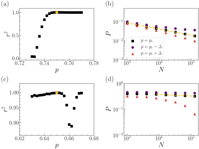
Figure S1: Estimation of the critical threshold in the conventional ensemble. (a) Coefficient of determination $r^{2}$ as a function of $p$. Here $C=1$. (b) Plot of $P$ as a function of $N$ at $p=p_{c}$, $p=p_{c}-\Delta$, and $p=p_{c}+\Delta$, respectively. We use $p_{c}=0.75$ and $\Delta=0.005$. Here also $C=1$. (c) Similar to (a) but for $C=\infty$. (d) Similar to (b) but for $C=\infty$. We use $p_{c}=0.65$ and $\Delta=0.01$. Detailed results can be found in Table S1.

VI Finite-size scaling analysis

VI.1 Conventional ensemble

We denote with $P(p,N)$ and $S(p,N)$ the values of the metrics of Eqs. (S3) and (S4), respectively, when exactly a fraction $p$ of edges is removed from the graph. To quantify the critical properties of the SPP transition, we rely on finite-size scaling (FSS) analysis [1] based on the scaling ansatzs

$$\langle P(p,N)\rangle=N^{-\beta/\bar{\nu}}F^{(1)}[(p-p_{c})N^{1/\bar{\nu}}]$$ (S7)

and

$$\langle S(p,N)\rangle=N^{\gamma/\bar{\nu}}F^{(2)}[(p-p_{c})N^{1/\bar{\nu}}]\;,$$ (S8)

where $\langle P(p,N)\rangle$ and $\langle S(p,N)\rangle$ are the ensemble averages of $P(p,N)$ and $S(p,N)$, respectively, $F^{(1)}(\cdot)$ and $F^{(2)}(\cdot)$ are universal scaling functions, while $\beta$, $\gamma$, and $\bar{\nu}$ are critical exponents for the percolation strength, the average cluster size, and the correlation volume, respectively. In Eqs. (S7) and (S8), $p_{c}$ is the critical value of the control parameter where the transition occurs in a network of infinite size. In a network of finite size $N$, the pseudo-critical threshold $p_{c}(N)$ indicates the value of the control parameter related to the biggest variation in the cluster structure of the network. There are multiple ways of defining this condition. We use

$$p_{c}(N)=\arg\max_{p}\,\left\langle S(p,N)\right\rangle\;.$$ (S9)

Still according to FSS, critical and pseudo-critical points are related by

$$p_{c}=p_{c}(N)+bN^{-1/\bar{\nu}},$$ (S10)

where $b$ is a constant.

VI.2 Critical properties of the shortest-path-percolation in the conventional ensemble

Note that we use a simplified notation to denote $\langle P(p,N)\rangle$ and $\langle S(p,N)\rangle$ in the figures, and in the text. Details on the notation are provided below.

We determine the value of the critical threshold $p_{c}$ using Eq. (S7). For $p=p_{c}$, the FSS ansatz predicts

$$P(p_{c})=\langle P(p=p_{c},N)\rangle\sim N^{-\beta/\bar{\nu}}\;,$$ (S11)

with $P(p_{c})$ highlighting the simplified notation adopted in the corresponding figure. Thus, we obtain the best estimator of the critical threshold as the value of the control parameter $p$ leading to the best power-law fit, Fig. S2. The best estimate of the $\beta/\bar{\nu}$ is obtained from the very same power-law fit. The ansatz of Eq. (S8) together with the estimated $p_{c}$ value further allows us to obtain the best estimate of $\gamma/\bar{\nu}$, i.e., $S(p_{c})=\langle S(p=p_{c},N)\rangle\sim N^{\gamma/\bar{\nu}}$, see Fig. S2(c).

For finite $C$, these scalings provide good estimates of the critical point and of the critical exponents. For infinite $C$, the estimates of the critical exponents are instead affected by strong finite size effects. The estimate of the critical point remains good.

Also, we estimate $\beta/\bar{\nu}$ and $\gamma/\bar{\nu}$ using the scaling

$$P_{c}(N)=\langle P(p=p_{c}(N),N)\rangle\sim N^{-\beta/\bar{\nu}}\;,$$ (S12)

$$S_{c}(N)=\langle S(p=p_{c}(N),N)\rangle\sim N^{\gamma/\bar{\nu}}\;,$$ (S13)

as predicted by Eqs. (S7), (S8) and (S10). $p_{c}(N)$ is defined in Eq. (S9). See Fig. S2(d) and (e) for details. These provide us with accurate estimates of the critical exponents for any $C$ value.

Finally, we perform the power-law fit of the expression $p_{c}-p_{c}(N)=bN^{-1/\bar{\nu}}$, see Eq. (S10), to determine the exponent $1/\bar{\nu}$ as well as the value of the constant $b$, Fig. S2(a). Numerical estimates of the critical parameters are reported in Table S1.

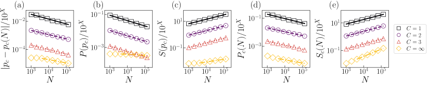
Figure S2: Finite-size scaling analysis in the conventional ensemble. An additional factor $10^{X}$ is used for visual clarity. We use $X=0,1,2,3$ for $C=1,2,3,N$, respectively. In each panel, we display as symbols the average value of the metric. Error bars are not displayed to avoid overcrowding the figure. Lines appearing in the plot are best fits obtained via simple linear regression on log-transformed variables, see text for details. (a) Scaling of Eq. (S10) to estimate $1/\bar{\nu}$. (b) Scaling at the critical point for the percolation strength, i.e, $P(p=p_{c})$ vs $N$, to estimate $\beta/\bar{\nu}$. (c) Scaling at the critical point for the average cluster size, i.e, $S(p=p_{c})$ vs $N$, to estimate $\gamma/\bar{\nu}$. (d) Scaling at the pseudo-critical point for the percolation strength, i.e., $P(p=p_{c}(N))$ vs $N$, to estimate $\beta/\bar{\nu}$. (e) Scaling at the pseudo-critical point for the average cluster size, i.e., $S(p=p_{c}(N))$ vs $N$, to estimate $\gamma/\bar{\nu}$. Estimated exponents are reported in Table S1.

			critical		pseudo-critical
$C$	$p_{c}$	$1/\bar{\nu}$	$\beta/\bar{\nu}$	$\gamma/\bar{\nu}$	$\beta/\bar{\nu}$	$\gamma/\bar{\nu}$
1	$0.750\pm 0.001$	$0.34\pm 0.02$	$0.326\pm 0.002$	$0.335\pm 0.001$	$0.31\pm 0.01$	$0.333\pm 0.002$
2	$0.701\pm 0.001$	$0.30\pm 0.01$	$0.325\pm 0.002$	$0.342\pm 0.001$	$0.28\pm 0.01$	$0.346\pm 0.001$
3	$0.682\pm 0.001$	$0.31\pm 0.01$	$0.328\pm 0.002$	$0.348\pm 0.001$	$0.29\pm 0.01$	$0.354\pm 0.003$
$\infty$	$0.650\pm 0.001$	$0.23\pm 0.01$	$0.060\pm 0.001$	$0.200\pm 0.002$	$0.23\pm 0.01$	$0.528\pm 0.002$

Table S1: Critical properties of the shortest-path-percolation (SPP) model. Estimates reported here are obtained via finite-size scaling analysis in the conventional ensemble.

VI.3 Event-based ensemble

Also here, we denote with $P(p,N)$ and $S(p,N)$ the values of the metrics of Eqs. (S3) and (S4), respectively, when exactly a fraction of $p$ edges is removed from the graph. The single-instance pseudo-critical point can be defined as in Ref. [23], i.e.,

$$p^{+}(N)=\arg\max_{p}\,\left[P(p,N)-P(p+2/N\bar{k},N)\right]\;,$$ (S14)

or as in Ref. [24], i.e.,

$$p^{-}(N)=\arg\max_{p}\,\left[P(p-2/N\bar{k},N)-P(p,N)\right]\;.$$ (S15)

In the above equations, the superscript $+$ ($-$) indicates whether the value of the control parameter $p$ is measured immediately after (before) the largest drop, induced by the removal of a single edge, in the value of the order parameter $P$ is observed. Note that the values $p^{+}(N)$ and $p^{-}(N)$ are measured for each individual realization of the SPP model. For such an individual realization, we can also measure the single-instance pseudo-critical value of the percolation strength, i.e.,

$$P^{+}(N)=P(p=p^{+}(N),N)\;.$$ (S16)

Similar definitions are valid for $P^{-}(N)$, and also for $S^{+}(N)$ and $S^{-}(N)$.

The best estimate of the pseudo-critical point under the event-based ensemble is obtained by taking the ensemble average of the single-instance pseudo-critical points of Eq. (S14), thus

$$p_{c}(N)=\langle p^{+}(N)\rangle\;.$$ (S17)

An analogous definition is obtained by using $p^{-}(N)$ in place of $p^{+}(N)$. The quantity defined in Eq. (S17) still obeys the same scaling relationship as of Eq. (S10). One can also measure the standard deviation of the single-istance pseudo-critical point, i.e.,

$$\sigma_{p_{c}}(N)=\sqrt{\langle\left[p^{+}(N)\right]^{2}\rangle-\left[\langle p^{+}(N)\rangle\right]^{2}}\;.$$ (S18)

Such a quantity obeys the scaling relation

$$\sigma_{p_{c}}(N)\sim N^{1/\bar{\nu}}\;.$$ (S19)

The single-instance pseudo-critical value $P^{+}(N)$ obeys the FSS distribution

$$\textrm{Prob.}\left[P^{+}(N)\right]=Q^{(1)}\left[P^{+}(N)\,N^{\beta/\bar{\nu}}\right]\;.$$ (S20)

For the average cluster size, we have instead

$$\textrm{Prob.}\left[S^{+}(N)\right]=Q^{(2)}\left[S^{+}(N)\,N^{-\gamma/\bar{\nu}}\right]\;.$$ (S21)

Here, $Q^{(1)}(\cdot)$ and $Q^{(2)}(\cdot)$ are universal scaling distributions. In particular, the average values of such distributions obey the scaling relationships

$$P_{c}(N)=\left\langle P^{+}(N)\right\rangle\sim N^{-\beta/\bar{\nu}}$$ (S22)

and

$$S_{c}(N)=\left\langle S^{+}(N)\right\rangle\sim N^{\gamma/\bar{\nu}}\;,$$ (S23)

respectively. Analogous scaling relationships are valid also for the standard deviation of the distributions $Q^{(1)}(\cdot)$ and $Q^{(2)}(\cdot)$, i.e.,

$$\sigma_{P_{c}}(N)=\sqrt{\left\langle\left[P^{+}(N)\right]^{2}\right\rangle-\left[\left\langle P^{+}(N)\right\rangle\right]^{2}}\sim N^{-\beta/\bar{\nu}}$$ (S24)

and

$$\sigma_{S_{c}}(N)=\sqrt{\left\langle\left[S^{+}(N)\right]^{2}\right\rangle-\left[\left\langle S^{+}(N)\right\rangle\right]^{2}}\sim N^{\gamma/\bar{\nu}}\;.$$ (S25)

All the above equations are valid also if we replace $P^{+}(N)$ with $P^{-}(N)$ and $S^{+}(N)$ with $S^{-}(N)$.

VI.4 Critical properties of the shortest-path-percolation in the event-based ensemble

The following applies regardless if one consider the definition of single-instance pseudo-critical point of Eq. (S14) or of Eq. (S15). Different estimates of the critical exponents are obtained either by using the scaling of the average of the various observables, or their standard deviations. The numerical results summarized in Tables S3 and S2 are organized accordingly.

We first determine the best estimate of the critical threshold using Eq. (S10). Here, both $p_{c}$ and $1/\bar{\nu}$ are treated as free parameters to perform the power-law fit. Also, we determine the critical exponent $1/\bar{\nu}$ using the scaling of Eq. (S19), see Fig. S4 (a) and Fig. S3 (a).

We then rely on the scaling laws of Eqs. (S22) and (S24) to determine the ratio between the critical exponents $\beta/\bar{\nu}$ and $\gamma/\bar{\nu}$, respectively, see Figs. S4 (b), (c), and Figs. S3 (b), (c). Additional estimates of these exponents are also obtained from Eqs. (S23) and (S25), see Figs. S4 (e), (f), and Figs. S3 (e), (f). Data collapse based on Eqs. (S20) and (S21) is provided in Fig. 3 of the main paper and in Fig. S5.

It’s worth mentioning that the two estimates of $1/\bar{\nu}$ obtained from Eqs. (S18) and (S19) are identical for finite $C$, but they differ for $C=\infty$. The latter finding is an agreement with the results of Ref. [24] for explosive percolation, with the caveat that the SPP estimate obtained from Eq. (S18) is smaller than the one obtained from Eq. (S19). The exact opposite was instead found for the case of explosive percolation.

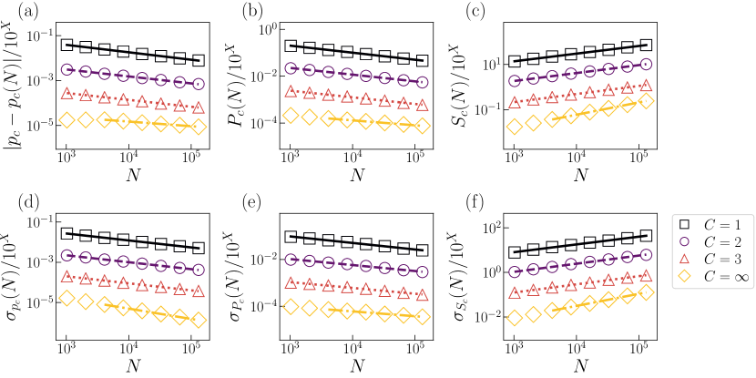
Figure S3: Finite-size scaling analysis in the event-based ensemble using the pseudo-critical point of Eq. (S14). Note that an additional factor $10^{X}$ was used for visual clarity. We use $X=0,1,2,3$ for $C=1,2,3,N$, respectively. In each panel, we display as symbols the average value of the metric. Error bars are not displayed to avoid overcrowding the figure. Lines appearing in the plot are best fits obtained via simple linear regression on log-transformed variables, see text for details. (a) Scaling of Eq. (S10) to estimate $1/\bar{\nu}$. (b) Scaling at the critical point for the percolation strength, i.e, $P(p=p_{c})$ vs $N$, to estimate $\beta/\bar{\nu}$. (c) Scaling at the critical point for the average cluster size, i.e, $S(p=p_{c})$ vs $N$, to estimate $\gamma/\bar{\nu}$. (d) Scaling of Eq. (S19) to estimate $1/\bar{\nu}$. (e) Scaling at the pseudo-critical point for the percolation strength, i.e., $P(p=p_{c}(N))$ vs $N$, to estimate $\beta/\bar{\nu}$. (f) Scaling at the pseudo-critical point for the average cluster size, i.e., $S(p=p_{c}(N))$ vs $N$, to estimate $\gamma/\bar{\nu}$. Estimated exponents are reported in Table S2.

		average			fluctuation
$C$	$p_{c}$	$1/\bar{\nu}$	$\beta/\bar{\nu}$	$\gamma/\bar{\nu}$	$1/\bar{\nu}$	$\beta/\bar{\nu}$	$\gamma/\bar{\nu}$
1	$0.750\pm 0.001$	$0.331\pm 0.002$	$0.301\pm 0.003$	$0.339\pm 0.003$	$0.346\pm 0.002$	$0.280\pm 0.006$	$0.348\pm 0.005$
2	$0.702\pm 0.001$	$0.310\pm 0.003$	$0.287\pm 0.004$	$0.351\pm 0.001$	$0.345\pm 0.002$	$0.256\pm 0.008$	$0.365\pm 0.004$
3	$0.683\pm 0.001$	$0.305\pm 0.002$	$0.284\pm 0.005$	$0.358\pm 0.003$	$0.349\pm 0.003$	$0.248\pm 0.008$	$0.367\pm 0.005$
$\infty$	$0.651\pm 0.002$	$0.206\pm 0.003$	$0.210\pm 0.001$	$0.545\pm 0.002$	$0.513\pm 0.004$	$0.206\pm 0.005$	$0.543\pm 0.004$

Table S2: Critical properties of the shortest-path-percolation (SPP) model in the event-based ensemble. Estimates reported here are obtained via finite-size scaling analysis in the event-based ensemble using the pseudo-critical point of Eq. (S14).

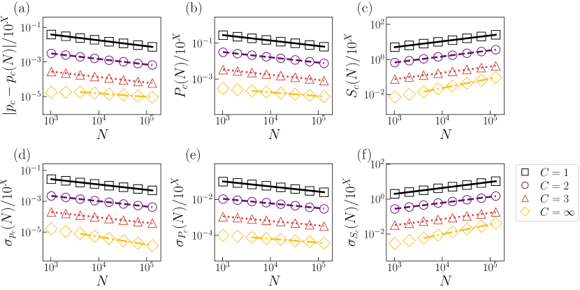
Figure S4: Finite-size scaling analysis in the event-based ensemble using the pseudo-critical point of Eq. (S15). Note that an additional factor $10^{X}$ is used for visual clarity. We use $X=0,1,2,3$ for $C=1,2,3,N$, respectively. In each panel, we display as symbols the average value of the metric. Error bars are not displayed to avoid overcrowding the figure. Lines appearing in the plot are best fits obtained via simple linear regression on log-transformed variables, see text for details. (a) Scaling of Eq. (S10) to estimate $1/\bar{\nu}$. (b) Scaling at the critical point for the percolation strength, i.e, $P(p=p_{c})$ vs $N$, to estimate $\beta/\bar{\nu}$. (c) Scaling at the critical point for the average cluster size, i.e, $S(p=p_{c})$ vs $N$, to estimate $\gamma/\bar{\nu}$. (d) Scaling of Eq. (S19) to estimate $1/\bar{\nu}$. (e) Scaling at the pseudo-critical point for the percolation strength, i.e., $P(p=p_{c}(N))$ vs $N$ to estimate, $\beta/\bar{\nu}$. (f) Scaling at the pseudo-critical point for the average cluster size, i.e., $S(p=p_{c}(N))$ vs $N$, to estimate $\gamma/\bar{\nu}$. Estimated exponents are reported in Table S3.

		average			fluctuation
$C$	$p_{c}$	$1/\bar{\nu}$	$\beta/\bar{\nu}$	$\gamma/\bar{\nu}$	$1/\bar{\nu}$	$\beta/\bar{\nu}$	$\gamma/\bar{\nu}$
1	$0.750\pm 0.001$	$0.339\pm 0.002$	$0.305\pm 0.003$	$0.335\pm 0.001$	$0.346\pm 0.002$	$0.284\pm 0.006$	$0.342\pm 0.003$
2	$0.702\pm 0.001$	$0.320\pm 0.003$	$0.293\pm 0.003$	$0.347\pm 0.002$	$0.345\pm 0.002$	$0.260\pm 0.007$	$0.345\pm 0.006$
3	$0.683\pm 0.001$	$0.317\pm 0.002$	$0.290\pm 0.004$	$0.359\pm 0.002$	$0.349\pm 0.003$	$0.254\pm 0.007$	$0.352\pm 0.004$
$\infty$	$0.650\pm 0.002$	$0.197\pm 0.003$	$0.212\pm 0.001$	$0.541\pm 0.001$	$0.513\pm 0.004$	$0.209\pm 0.005$	$0.558\pm 0.006$

Table S3: Critical properties of the shortest-path-percolation (SPP) model in the event-based ensemble. Estimates reported here are obtained via finite-size scaling analysis in the event-based ensemble using the pseudo-critical point of Eq. (S15).

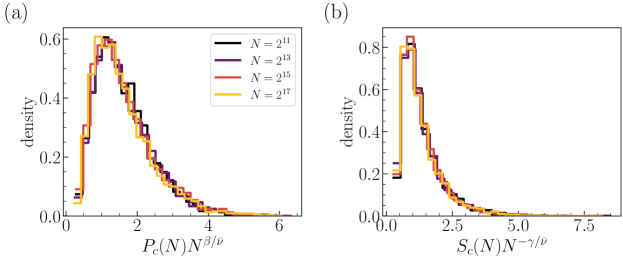
Figure S5: Shortest-path-percolation transition in the event-based ensemble. Here, we used $C=1$. (a) The distribution of ${P}_{c}(N)\,N^{\beta/\bar{\nu}}$ with $\beta/\bar{\nu}=0.301$. Different curves correspond to different network sizes $N$. (b) Same as in (a) but for $S_{c}(N)\,N^{-\gamma/\bar{\nu}}$ with $\gamma/\bar{\nu}=0.339$.

VI.5 Changing control parameter

VI.5.1 Mapping between control parameters

The two natural control parameters of the SPP model, i.e., $p$ and $t$, can be mapped one to the other using Eq. (S2). Typical results of this mapping are displayed in Fig. 4(a) of the main paper. For finite $C$, we find that the map can be written as

$$p=V\left(t\,N^{-\theta}\right)\;.$$ (S26)

Here, $V(\cdot)$ is a universal scaling function. An immediate way of estimating the exponent $\theta$ is to look at how $t_{c}(N)$ scales as function of $N$, see Fig. S6 (a). Also, we obtain another estimate of $\theta$ from the scaling of $t_{\max}(N)$, i.e., the total number of random origin-destination pairs that one has to extract in order to remove all edges from a ER network of size $N$, see Fig. S6 (b).

For infinite $C$, we find instead that

$$p=\left\{\begin{array}[]{ll}V^{-}(t\,N^{-\theta^{-}})&\textrm{ if }t\leq t_{c}(N)\\ V^{+}(t\,N^{-\theta^{+}})&\textrm{ if }t>t_{c}(N)\end{array}\right.\;,$$ (S27)

where $V^{-}(\cdot)$ and $V^{+}(\cdot)$ are universal scaling functions valid respectively for the supercritical and subcritical regimes of the SPP transition. A good estimate $\theta^{-}$ can be obtained by still looking at how $t_{c}(N)$ scales with $N$, see Fig. S6 (a). We determine the best estimate of $\theta^{+}$ from the scaling of $t_{\max}(N)$ vs $N$, see Fig. S6 (b).

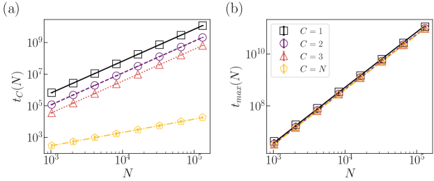
Figure S6: (a) $t_{c}(N)$ as a function of network size $N$ for different values of $C$. For each $N$ value, we plot the average values of $t_{c}(N)$ as symbols and the associated standard deviation as error bars. The scaling relation is given by $t_{c}(N)\sim N^{\theta}$ with $\theta=2.014\pm 0.002$ for $C=1$, $\theta=2.015\pm 0.001$ for $C=2$, $\theta=2.018\pm 0.001$ for $C=3$. For $C=\infty$, we fit $t_{c}(N)\sim N^{\theta^{-}}$ and obtain $\theta^{-}=0.843\pm 0.004$. (b) Maximum value of the raw number of demand $t_{max}(N)$ as a function of the network size $N$ for different values of $C$. The scaling relation is given by $t_{\max}(N)\sim N^{\theta}\,\log(N)$ with $\theta=2.091\pm 0.003$ for $C=1$, $\theta=2.073\pm 0.001$ for $C=2$, $\theta=2.070\pm 0.001$ for $C=3$. For $C=\infty$, we look at $t_{\max}(N)\sim N^{\theta^{+}}\,\log(N)$ and find $\theta^{+}=2.068\pm 0.004$.

VI.5.2 Critical properties of the shortest-path-percolation transition using the control parameter $t$

All the above theoretical arguments and numerical analyses generalize immediately if one replaces the control parameter $p$ with the control parameter $t$. Specifically, we look at the rescaled control parameter $\tilde{t}=tN^{-2}$ to deal with an intensive quantity similar to $p$.

Critical threshold values remain finite as along as $C$ is finite. A vanishing threshold is instead obtained for infinite $C$.

Due to the one-to-one mapping between $p_{c}(N)$ and $\tilde{t}_{c}(N)$, critical exponent values concerning the order parameter and the average cluster size are unaffected by the specific choice of the control parameter. For finite $C$, some variations are observed for the value of the exponent $1/\bar{\nu}$; these variations are, however, sufficiently small and likely due to finite-size effects. For infinite $C$, we recover $1/\bar{\nu}=2-\theta^{-}$. Results of the analysis are displayed in Fig. S7 and summarized in Table S4.

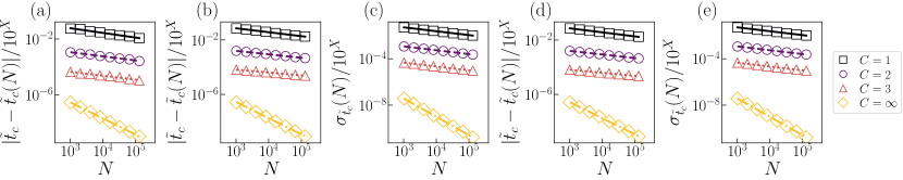
Figure S7: Finite-size scaling analysis with the control parameter $t$. Note that an additional factor $10^{X}$ is used for visual clarity. We use $X=0,1,2,3$ for $C=1,2,3,N$, respectively. In each panel, we display as symbols the average value of the metric. Error bars are not displayed to avoid overcrowding the figure. Lines appearing in the plot are best fits obtained via simple linear regression on log-transformed variables, see text for details. (a) Scaling of Eq. (S10) to estimate $1/\bar{\nu}$ in the conventional ensemble. (b) Similar to (a), but in the event-based ensemble using the pseudo-critical point $t_{c}(N)$ which corresponds to Eq. (S14). (c) Scaling of Eq. (S19) using the pseudo-critical point $t_{c}(N)$ which corresponds to Eq. (S14). (d) Similar to (b), but using the pseudo-critical point $t_{c}(N)$ which corresponds to Eq. (S15). (e) Similar to (c) but using the pseudo-critical point $t_{c}(N)$ which corresponds to Eq. (S15).

	conventional		event-based (Eq. S14)		fluctuation	event-based (Eq. S15)		fluctuation
$C$	$\tilde{t}_{c}$	$1/\bar{\nu}$	$\tilde{t}_{c}$	$1/\bar{\nu}$	$1/\bar{\nu}$	$\tilde{t}_{c}$	$1/\bar{\nu}$	$1/\bar{\nu}$
1	$0.693\pm 0.001$	$0.34\pm 0.01$	$0.696\pm 0.001$	$0.29\pm 0.01$	$0.335\pm 0.002$	$0.696\pm 0.001$	$0.298\pm 0.003$	$0.334\pm 0.002$
2	$0.124\pm 0.001$	$0.30\pm 0.01$	$0.126\pm 0.001$	$0.256\pm 0.004$	$0.332\pm 0.002$	$0.125\pm 0.001$	$0.27\pm 0.01$	$0.332\pm 0.002$
3	$0.039\pm 0.001$	$0.28\pm 0.01$	$0.040\pm 0.001$	$0.211\pm 0.005$	$0.331\pm 0.003$	$0.040\pm 0.001$	$0.220\pm 0.004$	$0.331\pm 0.003$
$\infty$	$0.000\pm 0.000$	$1.16\pm 0.01$	$0.000\pm 0.000$	$1.148\pm 0.003$	$1.59\pm 0.01$	$0.000\pm 0.000$	$1.186\pm 0.004$	$1.59\pm 0.01$

Table S4: Estimation of the critical threshold $\tilde{t}_{c}$ and of the critical exponent $1/\bar{\nu}$ when $\tilde{t}$ is used as control parameter to monitor the transition. For $C=\infty$, we estimate very small values of the threshold $\tilde{t}_{c}$, well below the numerical accuracy reported in the table.

VI.6 Effective infinite cost

We determine the effective value of the model parameter $C$ corresponding to the infinite-budget regime as follows. We consider the set of simulations of the SPP model with $C=N$. For each instance, we measure the value $Q_{max}=\max_{t}Q_{t}$ corresponding to the maximum distance observed between a pair of origin-destination nodes. We then take the average value of $Q_{max}$ over all SPP instances for a given network size $N$. We find that $Q_{\max}\sim N^{\delta}$, with $\delta=0.431\pm 0.001$ (see Fig. S8). Essentially, if $C$ increases towards infinity faster than $Q_{\max}$, then all pairs of selected nodes within the same connected component will lead for sure to the deletion of edges according to the rules of the SPP model.

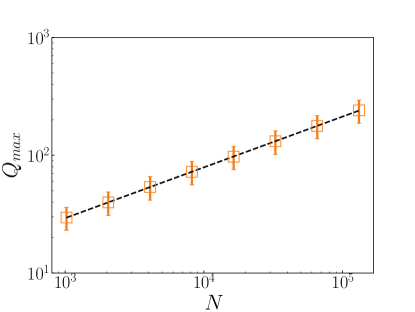
Figure S8: Maximum value of the shortest-path length $Q_{max}$ as a function of the network size $N$ for the shortest-path-percolation model with $C=N$. For each $N$ value, we plot the average values of $Q_{max}$ as symbols and the associated standard deviation as error bars. The scaling relation is given by $Q_{max}\sim N^{\delta}$ with $\delta=0.431\pm 0.001$. Best estimate of the critical exponent $\delta$ is obtained via simple linear regression on the log-transformed variables.

VI.7 Scaling of the size of the $k$-largest cluster

The scaling of Eq. (S22) valid for the relative size of the largest cluster applies also to the relative size of the $k$-th largest cluster, i.e.,

$$P^{(k)}_{c}(N)=\langle\max_{p}P^{(k)}(p,N)\rangle\sim N^{\beta/\bar{\nu}}\;.$$ (S28)

In Fig. S9, we show that the scaling holds for $C=1,2,3$ and $C=\infty$, for $k=2,3,4,$ and $5$. Estimated exponents are also reported in Table S5. As seen in Fig. S9 and Table S5, we could clearly obtain identical exponents from Eq. (S28).

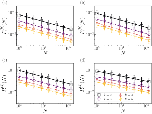
Figure S9: Scaling of the relative size of the $k$-th largest cluster. Results reported here are valid for $k=2,3,4$ and $5$. We display as points the average values of the relative size of the $k$-th largest cluster, and with the error bars their standard deviations. Here, we are using 100 samples. The different panels correspond to different values of the model parameter $C$. Specifically, (a) $C=1$, (b) $C=2$, (c) $C=3$, and (d) $C=\infty$. See Table S5 for detailed information.

$C$	$k=2$	$k=3$	$k=4$	$k=5$
1	$0.31\pm 0.01$	$0.32\pm 0.01$	$0.32\pm 0.01$	$0.32\pm 0.01$
2	$0.32\pm 0.01$	$0.33\pm 0.01$	$0.32\pm 0.01$	$0.33\pm 0.01$
3	$0.30\pm 0.01$	$0.30\pm 0.01$	$0.30\pm 0.01$	$0.31\pm 0.01$
$\infty$	$0.23\pm 0.01$	$0.23\pm 0.01$	$0.23\pm 0.01$	$0.23\pm 0.01$

Table S5: Estimation of the exponent $\beta/\bar{\nu}$ from Eq. (S28).