Oriented-grid Encoder for 3D Implicit Representations
Abstract
Encoding 3D points is one of the primary steps in learning-based implicit scene representation. Using features that gather information from neighbors with multi-resolution grids has proven to be the best geometric encoder for this task. However, prior techniques do not exploit some characteristics of most objects or scenes, such as surface normals and local smoothness. This paper is the first to exploit those 3D characteristics in 3D geometric encoders explicitly. In contrast to prior work on using multiple levels of details, regular cube grids, and trilinear interpolation, we propose 3D-oriented grids with a novel cylindrical volumetric interpolation for modeling local planar invariance. In addition, we explicitly include a local feature aggregation for feature regularization and smoothing of the cylindrical interpolation features. We evaluate our approach on ABC, Thingi10k, ShapeNet, and Matterport3D, for object and scene representation. Compared to the use of regular grids, our geometric encoder is shown to converge in fewer steps and obtain sharper 3D surfaces. When compared to the prior techniques, our method gets state-of-the-art results.
1 Introduction
There are many different ways of representing 3D surfaces. Implicit surface representations tell us that a point with coordinates , , and belongs to an object surface if , which defines the object. This type of 3D representation is advantageous since it is concise and guarantees continuity. Most learning-based 3D implicit representations start with encoding 3D points, then decoding their features into the chosen representation, defining . Two kinds of encoders are used, most of the times in parallel: i) mapping the 3D coordinates of each point alone to a higher dimensional vector space, here denoted as positional encoder; and ii) 3D points gathering information about their neighbors, named grid-based. Multi-layer Perceptrons (MLPs) are usually considered a suitable choice for decoders. This paper focuses on the grid-based encoders, as illustrated in Fig. 1.
Although many neural implicit 3D surface representation methods have been proposed, such as [20, 18, 36, 41, 53, 52, 28], previous techniques using geometric encoders still do not consider some of the object’s underlying geometric characteristics, like normals, and only utilize its spatial localization. Since 3D surface representation is bound to a specific object/scene, we should use all the object’s structural characteristics to model our geometric encoder. Therefore, we propose a novel-oriented multiscale grid-based encoder. We consider a tree representation with multiple Levels-of-Detail (LOD) that capture different detail resolution [52, 64]. In contrast, the grids are constructed at each level using the object’s surface occupancy and normals’ orientation. We then aim to answer the following research question: Does geometrically aligning the cell to the surface’s normal help in representation accuracy?
Our geometric encoder is the first to use surface orientations explicitly. From a multi-resolution surface representation, an abstract cell grid is aligned with the surface’s normal (deeper LOD will have better-aligned normals). In addition to the surface alignment, we add the assumption that regular (constructed) surfaces are locally planar (smooth surfaces). Taking this assumption, the grid alignment with the surface is locally defined up to a rotation around its vector’s normal surface, which we explicitly use to encode smoothness. The grid orientation and smoothness constraints are modeled by encoding features using cylinder grids, as shown in Fig. 1. Given the nature of the cylindrical coordinates (there are no corner-sharing features between neighboring grid cells), the new grid structure does not guarantee a smooth relationship between neighborhood cells. Thus, we propose using a shared 3D convolutional kernel for local feature aggregation. We summarize our contributions next:
-
1.
Oriented grids [Sec. 3.1]: A new sparse 3D tree representation aligning cells to the surface normals;
- 2.
- 3.
-
4.
Results show that our method obtains state-of-the-art surface representation while capturing the object’s structural regularity in more detail, lowering low-level roughness, and obtaining sharper 3D renderings.
2 Related Work
This section provides an overview of the related work on surface representation within the field of geometry processing, specifically from the perspective of our proposed method. We focus on geometric encoders, highlighting the differences concerning our method. We discuss various interpolation methods and list available pipelines for neural implicit representations.
Grid-based encoders: 3D object neural encoders can be represented as either feature-based or a combination of feature and grid-based. The feature-based methods [45, 46, 56, 43, 62, 47, 2, 5, 15, 7, 63, 12, 41, 36, 44, 43, 13, 19, 61, 4, 23], encode a feature representation of a dataset of objects from the input point clouds and decode them to the desired output representation. Typically, such encoders have a large memory requirement and are more applicable in generalizability across all objects, often at the cost of quality. As a result, these methods frequently generate overly smoothed objects that lack intricate details. This paper focuses on 3D object implicit representation [50, 28, 53, 13], that is, object bounded and not a general object encoder.
Recent advancements in neural representations [37, 55] have led to the widespread use of encoders that combine grids and feature-based approaches. These grid-based encoders use a 3D grid to simplify the feature space and create an explicit 3D embedding [36, 44]. Recent works used grid-based encoders for neural 3D representations [17, 53, 28, 10]. These representations allowed the construction of a per-object implicit representation while preserving far more details. More recent approaches have employed multiscale representations, such as octrees [48, 56, 58, 57, 59, 64, 52]. They can a capture higher level of information in data structures [14, 27]. Plenoctrees and NGLOD [64, 52] leverage the octree representation to achieve a smaller model and capture multiple resolutions of the 3D object. Instant-NGP [38] employs the octree representation with hash encoding to various tasks, including 3D object representation, and has demonstrated improved training efficiency. Due to the success of multiscale representation, we use a tree-based representation, which decimates the original mesh into a set of grids for each LOD, according to an octree.
Interpolation: Aggregating features to capture local or global information about 3D objects is critical. Approaches that require a grid representation often use interpolation as an aggregating tool due to its simplicity and effectiveness. For instance, [36, 32, 44, 51, 24, 31, 55, 40, 17] use trilinear interpolation to obtain features per query inside a cell. [17] discusses interpolation schemes, concluding the superior performance of trilinear interpolation over the nearest neighbor approach leading to optimal training convergence that is robust to different learning rate hyperparameters.
Similarly, multiscale grid features [64, 52, 38] are obtained per LOD in an octree representation using trilinear interpolation, following the same principle. The encoder grid space can be trained in a coarse-to-fine fashion, i.e. the features are trained using a per-level MLP for the same query point, where the corners for each cell are shared among levels. The common factor in these approaches is that all exploit grids’ regularity, making trilinear interpolation a natural choice. Due to the orientated cell property of our geometric encoder, we propose a new cylindrical interpolation scheme inspired by trilinear interpolation, along with a 3D sparse convolutional kernel shared among all LODs. The former warrants feature invariance between anchor rotations (since they are estimated up to a rotation) and the latter smoothness between neighboring cells and levels.
Decoders and Tasks: The oriented-grid encoder proposed in this paper can be applied to any type of decoder and representation task for implicit representations of 3D objects. In neural implicit methods focusing on per-object representation, the decoder typically consists of a small number of MLPs and employs a geometric grid-based encoder [50, 52, 35, 55, 40, 53, 28, 33].
In this work, the goal is to model the 3D representation to a surface mapping parameter. To this extent, the most commonly used ones are SDFs [22, 6, 11, 41, 16, 55, 24, 30], occupancies [11, 36, 7, 39, 44, 29, 54, 40], or unsigned distance fields [13, 19, 33]. Once modeled, the mesh is reconstructed using the marching cubes algorithm [34] or raytracing [1, 21] to render images from different viewpoints. Once the oriented octree grid is built, we generate a mesh representation from a point cloud. Our approach is agnostic to any output representation.
3 Oriented grid encoder
In the 3D implicit representation pipeline, a single 3D point passes through a geometric encoder, positional encoder, or both. The features are then injected into a decoder that models the object’s surface, as in Fig. 1. Repeating the process for all point cloud points obtains a sparse output representation with respect to the modeled 3D surface.
The paper focuses mainly on the 3D grid encoder, specifically, the geometric grid encoder (orange block in Fig. 3), detailed in this section. The input is a point and the pre-initialized trees that best fit the object. The output is a set of LOD tree features. We start by constructing the trees in Sec. 3.1. The features extracted from the trees are aggregated locally, crossing neighboring information (see Sec. 3.3). The aggregated features are used in the cylindrical interpolation scheme proposed in Sec. 3.2.
3.1 Oriented grids construction
Similar to previous works [14, 27, 56, 57, 52, 64], we use an octree representation to model the grid-based 3D encoder. However, in addition to the standard eight actions for splitting a grid into eight smaller ones in the subsequent LODs, we include rotation actions to model cell orientations, where at the higher levels a smaller (tighter) grid and a finer alignment better represent the object, as shown in Fig. 2. Instead of modeling each action individually, which would result in a branching factor of 56 — – per subsequent LOD, and since grid size and orientation are independent, we split them into two trees:
-
Tree 1:
Structured octree for modeling the sizes of the grids; and
-
Tree 2:
Orientation tree for modeling the cell orientation.
For the structured octree in Tree 1, its representation consists of LODs , bounded within . We followed the typical octree modeling [52, 64].
Orientation tree: For a normalized point taken from the object’s surface point cloud, we associate a normal to this query111We can either get the normal from a 3D oriented point cloud or estimate it from neighboring 3D points., denoted as . The goal is to align the cells along the surface in a coarse-to-fine manner. To maintain consistency within the LODs, we construct a set of normal anchors representing the finite possible set of orientations per level. We then rotate the cells such that the -axis matches the anchor, which is the closest anchor to the query normal . To model a searching tree [49], one needs to define: i) the node state, ii) the actions, iii) state transition, and iv) initial state:
-
•
The node state denoted as is defined by a set of three 2-tuple elements:
(1) where superscripts and indicate the lower and higher angle range limits.
-
•
We have seven possible actions:
(2) - •
-
•
The initial state is set as .
We conclude orientation tree modeling by defining rotations. A rotation is obtained per LOD and cell from state . The rotation anchor is computed from the states’ Euler angles range , where . To compute the state for each cell, we allow the rotation anchors to align the –axis of the cell with the surface normal, using cosine similarity, up to a rotation222Multiple solutions from the search can align to the surface normal. Since we restrict the alignment of the normal to the –axis, the and axes can move freely. An example of this can be seen in the supplementary material..
Grid to query point association: Each cell in Tree 1 has a fixed orientation computed from searching Tree 2. During training and evaluation, a query point is associated with a cell in Tree 1 (structured tree) on a particular LOD. Then, the cell is rotated using the corresponding rotation anchor. We note that a point may be outside all octree cells. In this case, we discard the query.
We note that the normal of the input points is not used in the model; the normals are only used to construct the oriented grid. Also, the orientation tree, from low-to-high LODs, will incorporate a coarse-to-fine approximation to the input normals. This means that the orientation tree will be mostly invariant to small noise levels. At lower LODs, rotations obtained by noisy and noiseless normals might differ slightly. In addition, we highlight that this work aims to build an implicit representation of an object. The normals used to construct the encoder are typically accurate. During training and evaluation, we use the cell’s anchor normal.
3.2 Cylindrical interpolation
While trilinear interpolation has been the typical way of obtaining the features for regular grids [55, 40, 64, 52], for oriented grids, using the same approach as regular grids is not appropriate since the cells do not share corners between neighbors (cells are rotated). There is rotation ambiguity in the –axis. So, we propose to use oriented cylinders, as shown in Figs. 1 and 3, that can exploit the alignment of the cells and mitigate the lack of invariance in defining the grid orientation, as discussed above. An example can be seen in the supplementary material. This rotation invariance adds an explicit smoothness constraint to points inside the grid.
Given the query point, the objective is to compute relative spatial volumes for feature coefficients, considering the point’s relative position within the cylinder. Cylindrical interpolation coefficients measure the closeness of the point to the extremities of the cylinder cell representation, as depicted in Fig. 4. A point closer to the top and the border of the cylinder will produce a lower volume for that boundary (yellow volume). Therefore, its distance from the opposite face will be high, thus, a higher volume coefficient (green volume). The highest coefficient in this example will be the opposite according to the center axis (blue volume). Finally, the volumetric interpolation gives us three coefficients, , , and (see Fig. 4 for derivation). With these coefficients, learnable features , where , per cell333For simplicity, we omit the cell index. and per LOD , are used to interpolate the query point features (linear combination): .
3.3 Local Feature Aggregation
The features obtained solely by the proposed interpolation scheme lack neighborhood and LOD information. In contrast to trilinear interpolation, where the features from the corners of the interpolation cell are shared among neighbors and levels, cylindrical interpolation does not inherently incorporate knowledge between its neighborhood and other LODs. Thus, we propose the usage of a shared across levels 3DCNN for local feature aggregation, here denoted as . The convolutional kernel per feature level is shared across the tree. For each feature at each cell, there is an associated kernel :
| (5) |
where is the set of neighborhood cells. We utilize a 3D sparse convolution, i.e. the neighbor is ignored if it is not present. The neighborhood comprises neighbor cells within the kernel, with the current cell as the center.
4 Implementation
Sec. 4.1 presents the encoder creation, used decoder architectures, and output representations. Section 4.2 describes the training and evaluation procedures, and Sec. 4.3 details the experiments.
4.1 Architecture encoder and decoders
Encoder: The dual-tree construction used to encode an object is a pre-processing operation. Different noise levels are added to the input points, following the standard protocol [52]. This representation retains the LOD cells to which the object belongs and the respective anchor orientation. Each cell has its corresponding features, as described in Sec. 3.2. During training and evaluation, a point is queried, and the features are extracted and passed to the decoder.
Decoders and output representations: We use an MLP-based architecture as a decoder for the implicit representation. The decoder is trained at each level and shared across all LODs. Besides the input interpolated feature, we add a positional encoder [37] on the point with frequencies, as well as on the anchor’s normal with frequencies. The point and the normal are attached to each positional encoder, with the size of and . We show our method for SDF and occupancy as output representation.
4.2 Training and Evaluation
During the training stage, we sample points from the input point cloud, determine where they lie in each LOD, and interpolate their features accordingly to the chosen voxels. We compute the sum of the squared errors of the predicted samples or the cross-entropy from the active LODs for SDF and occupancy, respectively. Additionally, we estimate the normals from the gradient [40, 39]. Then, we compute the L2-norm between the computed normals and the anchor normals as a regularization term, weighted by . The two terms are added to obtain the final loss.
During the evaluation, we obtain uniformly distributed input samples from a unit cube with resolution . We show results for the last LOD , corresponding to finer LOD. The input query gets discarded if it doesn’t match an existing octree cell. Finally, we obtain the mesh from the output using marching cubes [34].
4.3 Experimental Setup
Following prior works, we evaluate our 3D reconstruction quality using Chamfer Distance (CD), Normal Consistency (NC), and Intersection over Union (IoU) for each object. The CD is computed as the reciprocal minimum distance for the query point and its ground truth match. We compute CD five times and show the mean. NC is the corresponding normals computed from the cosine similarity between the query normal (corresponding to the query point obtained during CD calculation) and its corresponding ground truth normal. We report the NC as a residual of the cosine similarity between both normals. IoU quantifies the overlap between two grid sets.
Datasets: We evaluate our method on three different datasets, ABC [26], Thingi10k [65], and ShapeNet [9]. We sample 32 meshes each from Thingi10k and ABC and 150 from ShapeNet. We watertight ShapeNet meshes using [60]. This work is implemented in PyTorch [42].
Model: Our decoder architecture has one hidden layer of dimension , with ReLU. Each voxel feature is represented as a dimensional feature vector. The positional encoding for the query point and normal are represented with frequencies. We consider the sparse 3D convolutions for local feature aggregation, with a kernel size , . The cylinder radius was empirically set to . Further parameter investigations are shown in the supplementary material.
Using the Adam optimizer [25], we train our model for up to epochs, with a learning rate of and . An initial sample size of points is considered, with a batch size of . Resampling is done after every epoch. The points are sampled from the surface and around its vicinity in equal proportions. It is also ensured that each voxel has at least 32 samples before surface sampling. We consider the LODs for all the datasets.
Baselines: We compare our approach against state-of-the-art approaches frequency-based encoders BACON [28], SIREN [50] and Fourier Features (FF) [53], and 3D sparse network NDF [13], which were trained with the supplied settings. We simplify NDF [13] by voxelizing the point cloud and obtain the surface using marching cubes, using the same settings from Sec. 4.2, instead of their ball pivoting algorithm [3]. We also evaluate a regular grid direct approach against our method, where we adapt [52], which required smaller changes in our pipeline for a fair comparison against the oriented grids (see the supplementary materials for details). The surface reconstruction setup was the same for all methods, described in Sec. 4.2.
ccccc ccc[code-before =\rectanglecolorGray!201-12-8]
Network options
Results
Trilinear
Interpolation
Cylindrical
Interpolation
3DCNN
3x3x3
3DCNN
5x5x5
Normals
Regularization
CD NC IoU
✓ 1.278 4.410 0.881
✓ 0.570 4.348 0.990
✓ ✓ 0.434 4.094 0.998
✓ ✓ 0.431 4.093 0.998
✓ ✓ ✓ 0.443 4.058 0.998


5 Experiments
Ablations are presented in Sec. 5.1, where we evaluate the different stages of our method. Section 5.2 shows the direct comparison between regular and oriented grids. Finally, we evaluate our method against methods using different encoder strategies in Sec. 5.3.
5.1 Ablations
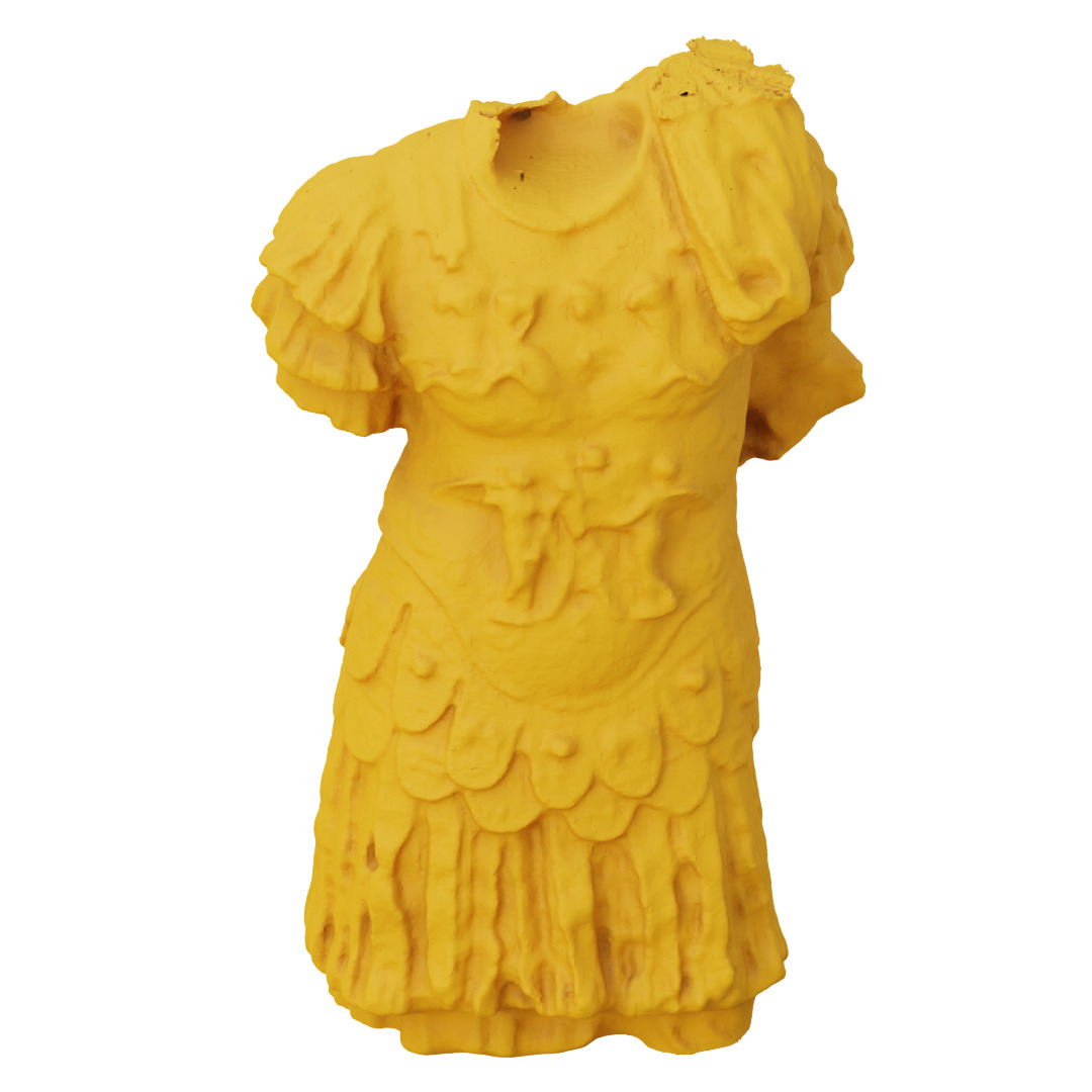
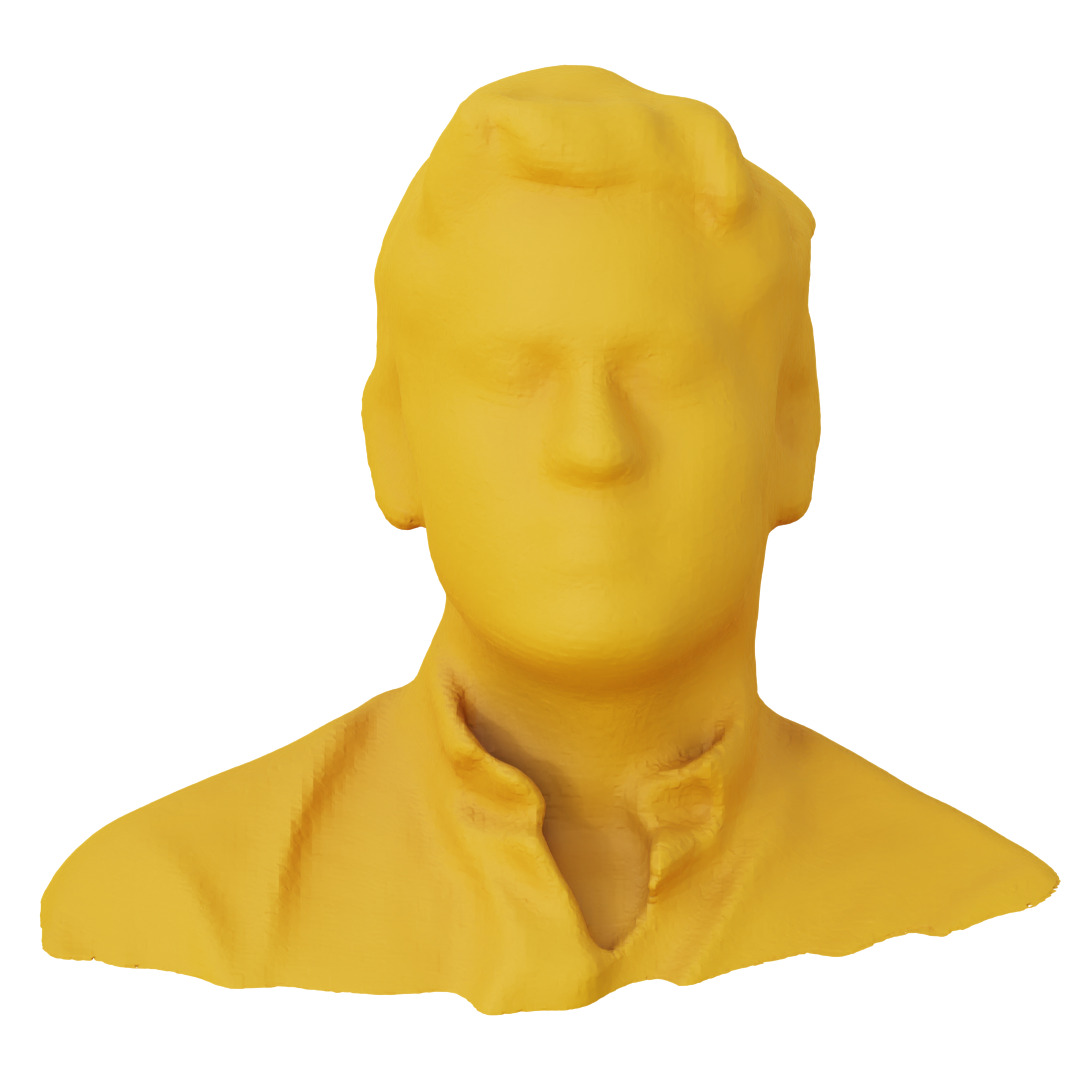
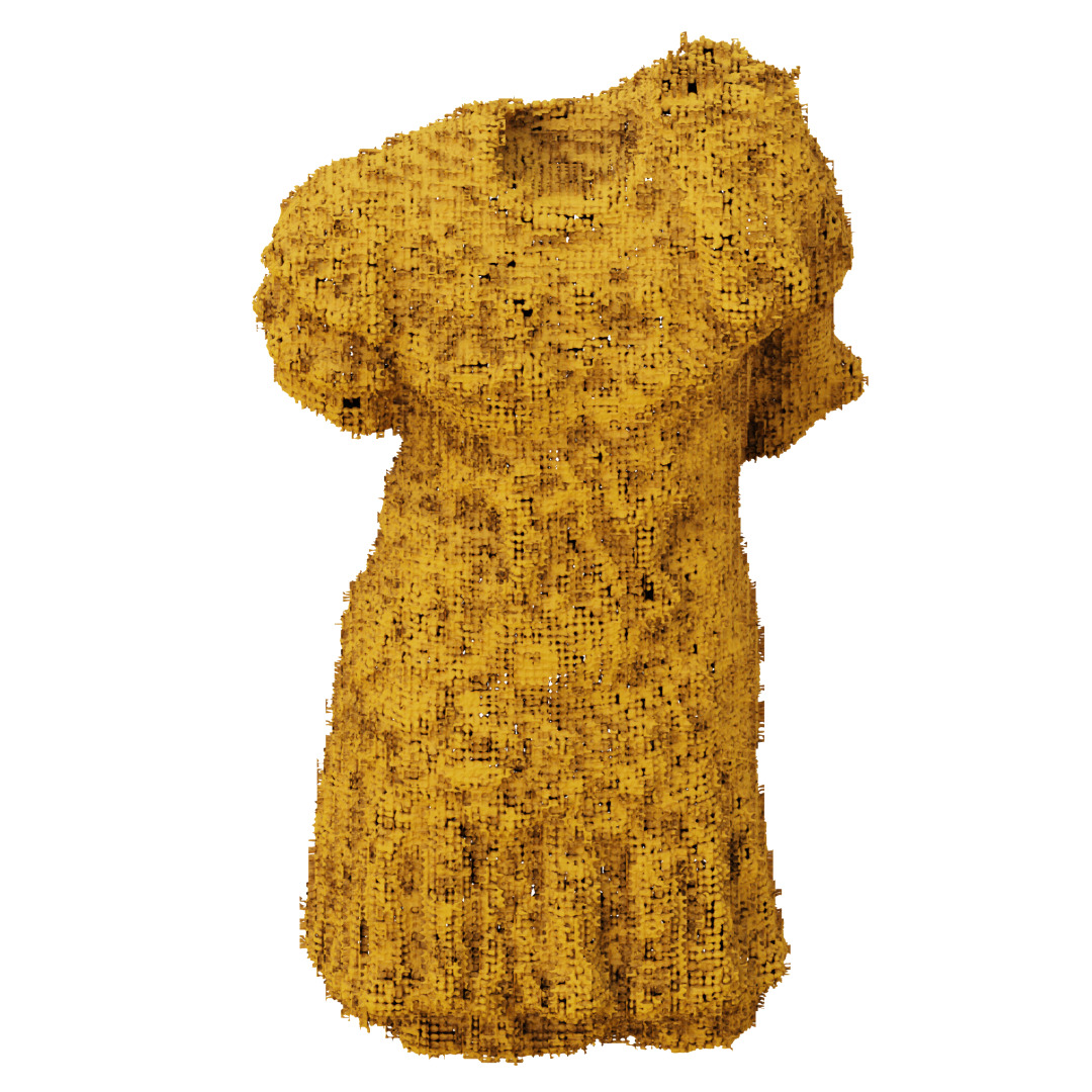
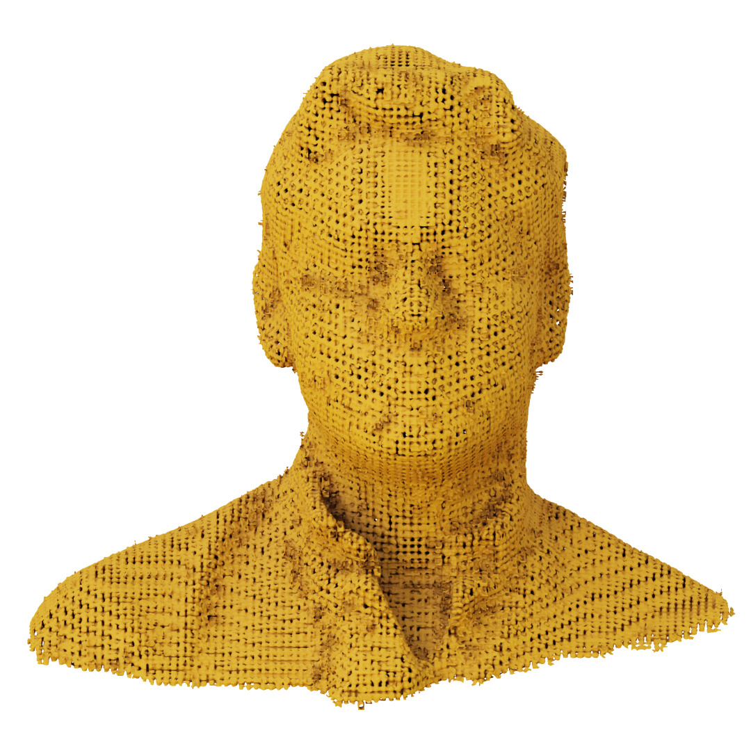
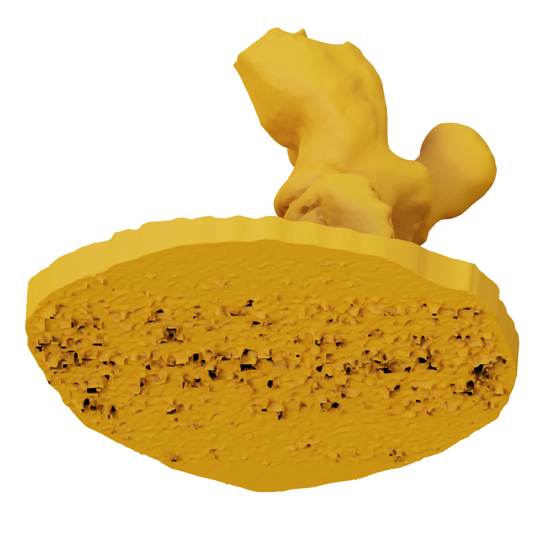
We gradually add changes to different pipeline blocks to analyze each component’s relevance. Ten meshes from ABC and Thingi10k datasets are randomly sampled for training and testing. Figure 4(e) shows different cases listed in Sec. 4.3, based on the changes made to encoder. We notice that using oriented grids with trilinear interpolation results in many holes. Since cells are rotated per the anchor normal, we use a rotation-invariant cylindrical representation for interpolation. Though rougher, this yields a more adapted representation (significant improvement in CD).
We see a significant improvement in the mesh smoothness (reflected in NC) with the addition of 3DCNN (Fig. 4(e) LABEL:sub@subfig:333cnn and LABEL:sub@subfig:555cnn), effectively contributing to the local feature aggregation step. Our experiments show that the kernel of achieves better performance, preferred for subsequent experiments. The proposed normal regularization enhances smoothness but sacrifices accuracy. Additional ablations are discussed in the supplementary material.
ccccccc[code-before =\rectanglecolorGray!201-12-7]
Network options
Results
Regular
Grids
Oriented
Grids
SDF
Decoder
Occupancy
Decoder
CD NC IoU
✓ ✓ 0.445 4.257 0.997
✓ ✓ 0.687 4.117 0.989
✓ ✓ 0.788 4.140 0.995
✓ ✓ 0.443 4.058 0.998
 &
& 


5.2 Regular vs. Oriented grids
Section 5.1 compares the performance of our method with regular grids on SDF and occupancy decoders. SDF and occupancies decoders are trained as explained in Sec. 4. Normal regularization remains the same for both cases. Our method outperforms regular grids with an SDF decoder on all fronts, yielding smoother results on structured surfaces. Despite the underperformance of the occupancy framework, we observe fewer holes and dents (with the latter having a significant impact on the IoU), as shown in the supplementary material. These results show the adaptability of our method to different decoder output representations.
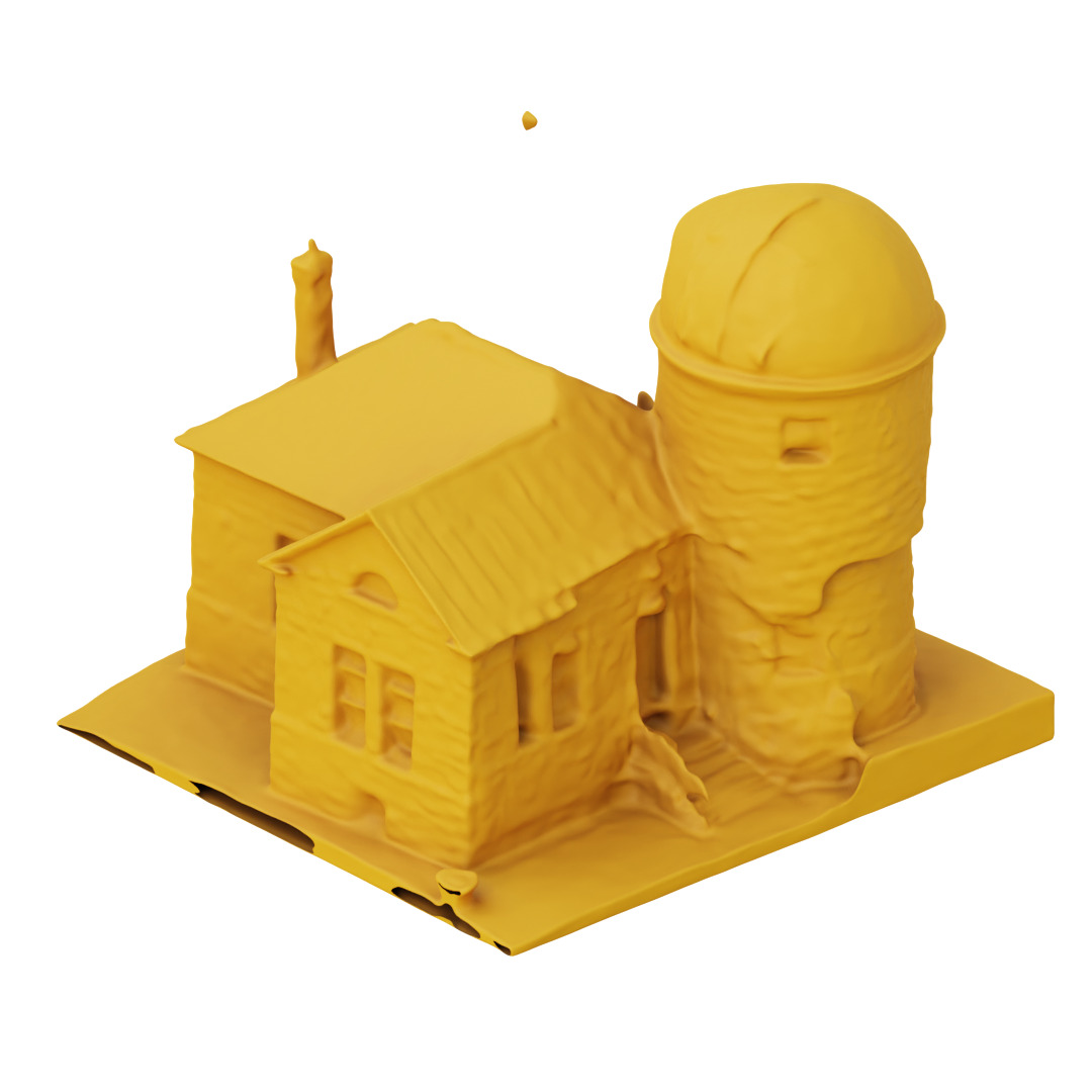
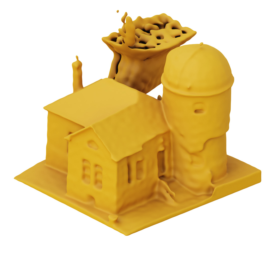
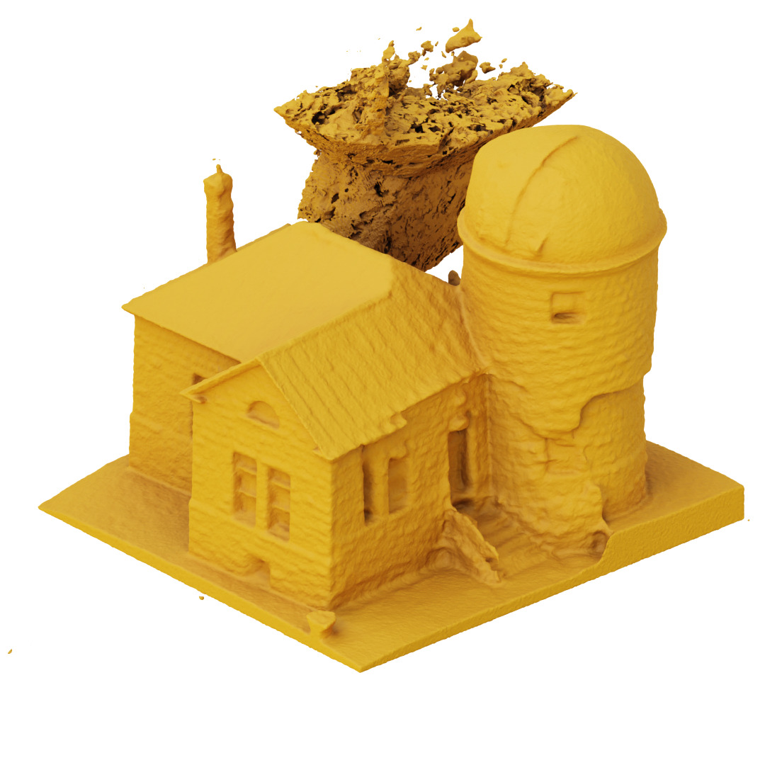
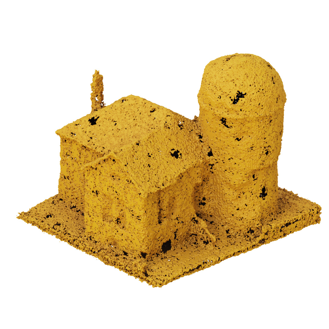
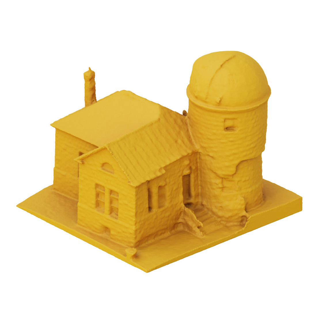
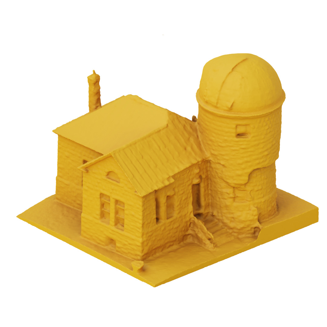
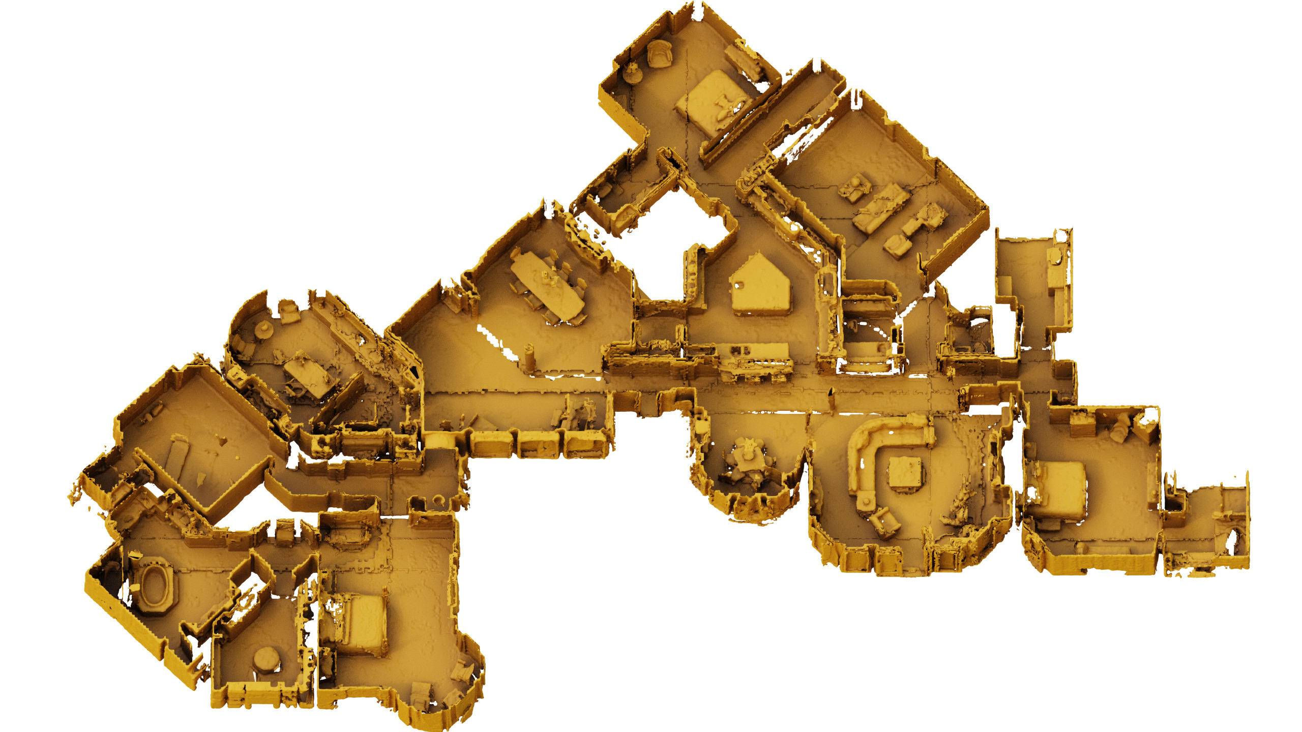
To open possible extensions of our work to large-scale scene representation, we show the render of our method on a scene from Matterport3D [8]. We divide the scene into crops (with ground plane included) and train a model with an occupancy decoder for each crop. During inference, the mesh crops are rendered using marching cubes and finally fused to yield the scene, as shown in Fig. 6. Regular grids render a rougher and muddled 3D representation. Our method adapts well to thin surfaces and renders the scene with less roughness and sharper quality. Additional scenes are shown in the supplementary material.
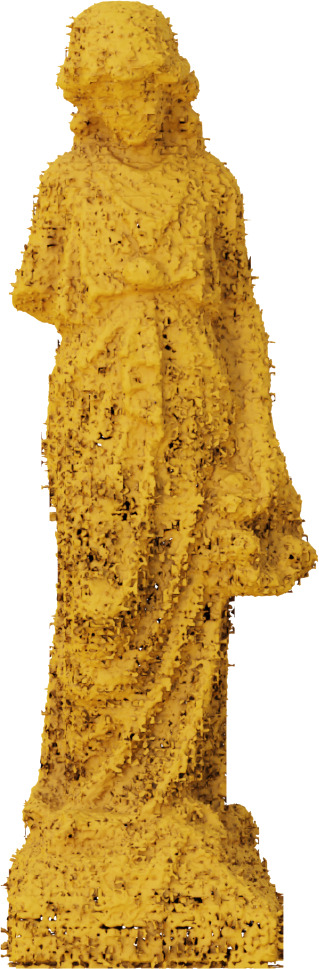
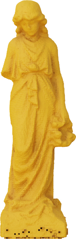
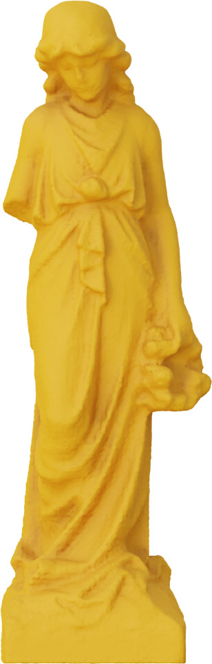
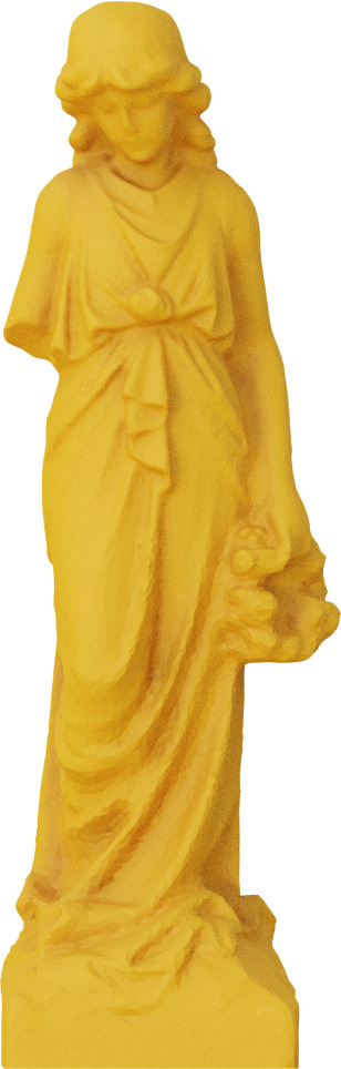
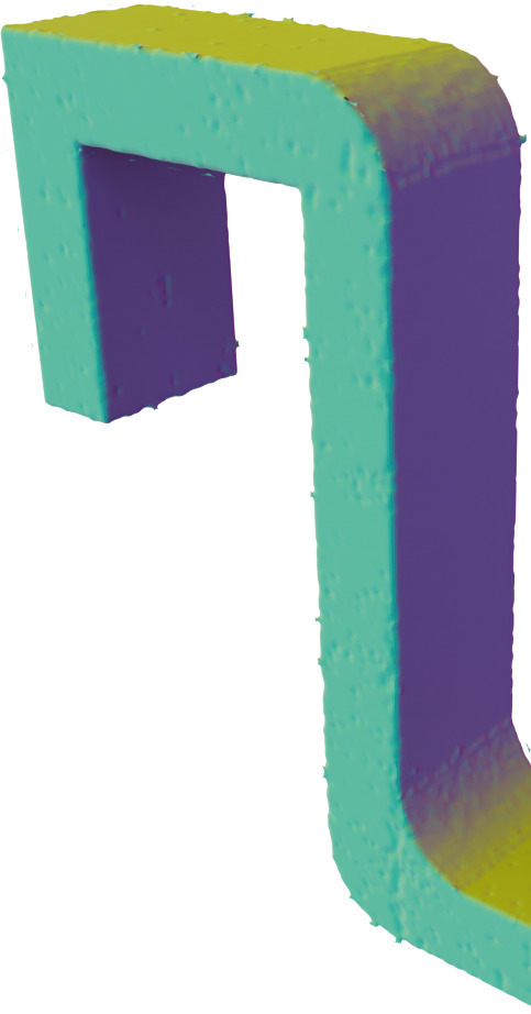
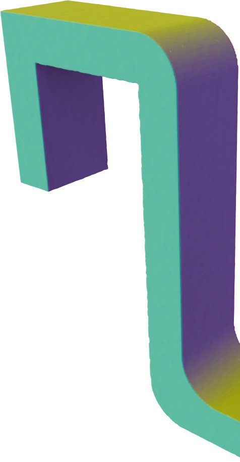
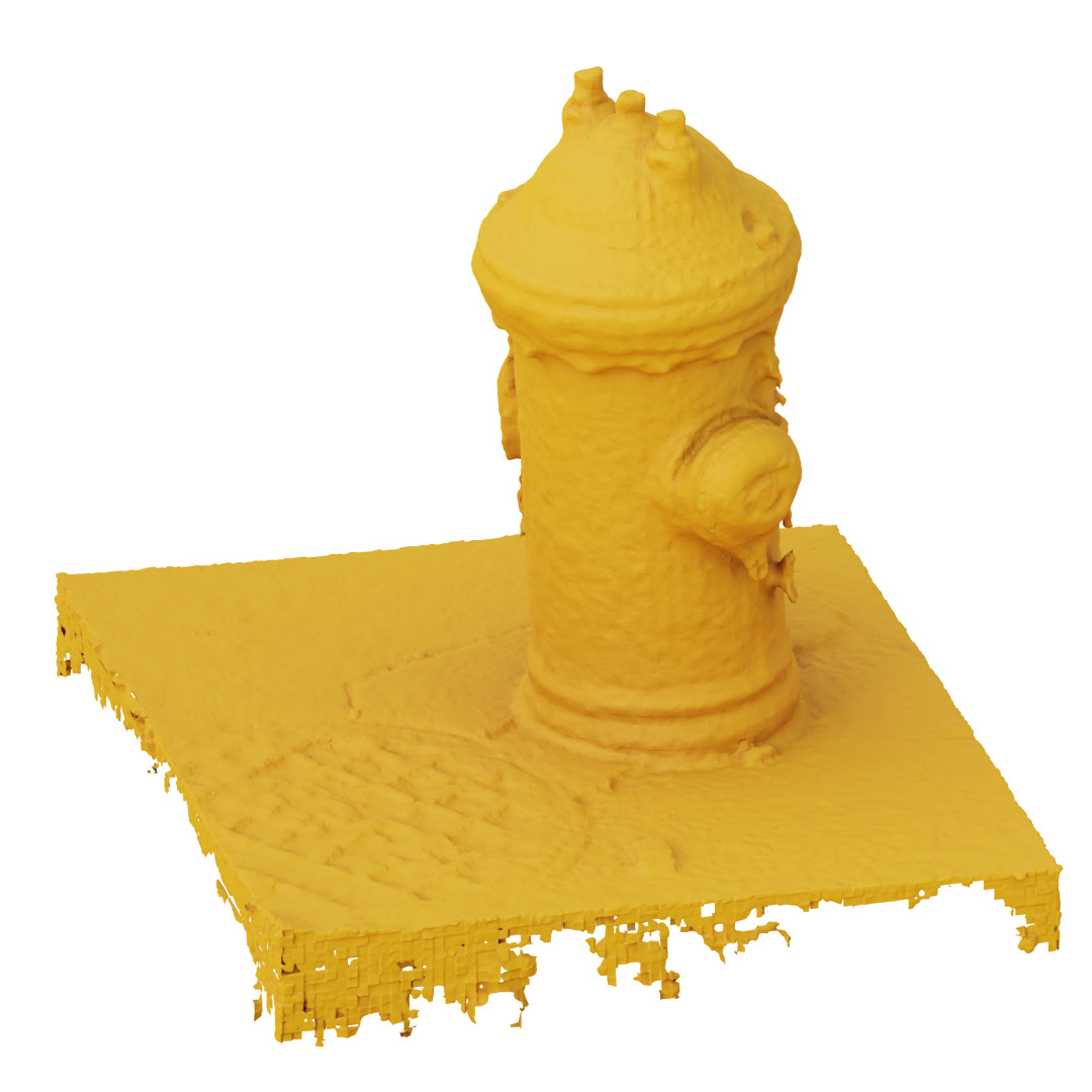
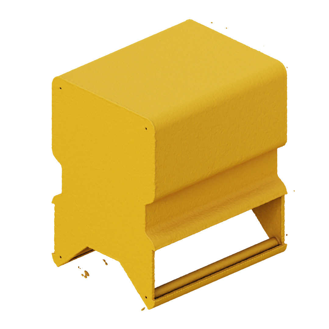
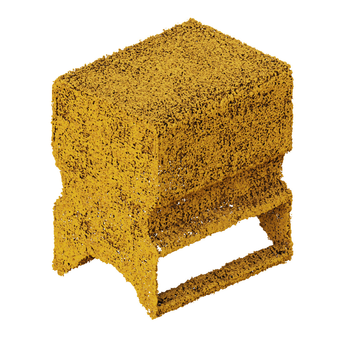
As a consequence of the oriented grids, we observe that the proposed encoder renders planar surfaces more effectively in fewer training steps. Especially in more structural regular objects, the regular grids produce a caustic-like effect (surface noise). We observe a noise reduction in the surface reconstruction for the oriented grids, as seen in Fig. 7 as soon as the first epoch. More results per epoch can be seen in the supplementary material.
5.3 Baselines
Quantitative Results: Section 5.3 details the experimental results of our method against the baselines. We infer that grid-based methods outperform the baselines with significant improvement on all fronts. In a simple dataset composed of planar objects, like ABC, our encoder reconstructs smoother planar surfaces due to the alignment of the oriented grids. While rendering holistic details, most baselines often have over-smoothed surfaces. We also observe a higher IoU for our method due to fewer holes in our mesh and negligible splatting (many small mesh traces around the sampling region). Overall, the oriented grids produce robust 3D representations with higher fidelity across all datasets.
We also provide the number of parameters required for rendering the mesh. The advantage of multi-resolution grid representations is that the decoder size can be reduced to just an MLP with one hidden layer. This results in our approach getting meshes faster than other methods.
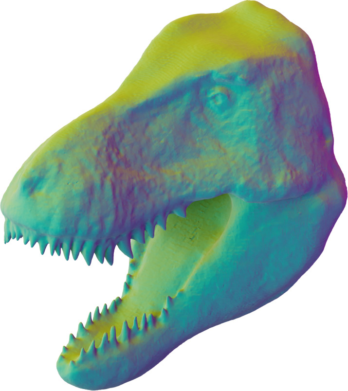
Qualitative Results: Illustrative examples from Thingi10k and ShapeNet datasets are shown in Fig. 8. While BACON and FF can model the object with reasonable accuracy, it registers a lot of splattering, giving rise to unwanted noisy surfaces and artifacts. SIREN and BACON produce over-smoothed surfaces, losing intricate details on the mesh. NDF produces a lot of holes but manages to get compact meshes without splattering. BACON, SIREN, and FF collapse on the ShapeNet dataset. We note that we tried both watertight and not watertight versions of ShapeNet, but we obtained similar results for the failing baselines. We suspect these methods fail on ShapeNet due to their reliance on frequency-based encoding, which fails in high-frequency shape settings, e.g. the small gaps in the chair.
@lccccc[colortbl-like] \rowcolorGray!40
SIREN
[50]
BACON
[28]
FF
[53]
NDF
[13]
Ours
\rowcolorGray!10 Results for the ABC dataset [26].
\rowcolorGray!10 CD 5.837 2.229 18.98 5.020 0.603
\rowcolorGray!10 NC 5.150 4.658 5.170 4.732 3.987
\rowcolorGray!10 IoU 0.879 0.987 0.916 0.950 0.998
Results for the Thingi10k dataset [65].
CD 62.85 60.72 67.93 4.421 0.608
NC 49.11 5.052 58.31 4.636 4.413
IoU 0.716 0.928 0.877 0.920 0.995
\rowcolorGray!10 Results for the ShapeNet dataset [9].
\rowcolorGray!10 CD – – – 4.125 0.392
\rowcolorGray!10 NC – – – 6.186 5.425
\rowcolorGray!10 IoU – – – 0.984 0.999
Number of Inference Parameters
# Params. 199K 537K 527K 4.62M 388K
Limitations: Small holes can arise from non-watertight planar surfaces that affect both oriented and regular grids. The oriented grid, however, fills holes more adequately than the regular counterpart. A more general multi-resolution grid representation issue is the difficulty of modeling thin surfaces. Despite the limitation, our method substantially improves from the regular grid. We provide meshes for such cases in the supplementary material. We hope to study and mitigate the above limitations in subsequent works.
6 Conclusion
This paper proposes a novel approach for a 3D grid-based encoder for 3D representation. The encoder considers the inherent structural regularities in objects by aligning the grids with the object surface normal and aggregating the cell features from a newly developed cylindrical interpolation technique and local aggregation scheme that mitigates the issues caused by the alignment. Oriented grids yielded state-of-the-art results while being more robust and accurate to decoder representation changes, answering the paper’s research question. Future work lies in extending the work for neural radiance fields and scene and object reconstruction where the object implicit representation is unknown.
Acknowledgements: Gonçalo was partially supported by the LARSyS funding (DOI: 10.54499/LA/P/0083/2020, 10.54499/UIDP/50009/2020, and 10.54499/UIDB/50009/2020) and grant PD/BD/150630/2020, from the Portuguese “Fundação para a Ciência e a Tecnologia”.
References
- [1] John Amanatides. Ray tracing with cones. SIGGRAPH, 18(3):129–135, 1984.
- [2] Benjamin Attal, Selena Ling, Aaron Gokaslan, Christian Richardt, and James Tompkin. Matryodshka: Real-time 6dof video view synthesis using multi-sphere images. In European Conf. Computer Vision (ECCV), pages 441–459, 2020.
- [3] Fausto Bernardini, Joshua Mittleman, Holly Rushmeier, Cláudio Silva, and Gabriel Taubin. The ball-pivoting algorithm for surface reconstruction. IEEE Trans. on Visualization and Computer Graphics, 5(4):349–359, 1999.
- [4] Alexandre Boulch and Renaud Marlet. Poco: Point convolution for surface reconstruction. In IEEE/CVF Conf. Computer Vision and Pattern Recognition (CVPR), pages 6302–6314, 2022.
- [5] Michael Broxton, John Flynn, Ryan Overbeck, Daniel Erickson, Peter Hedman, Matthew Duvall, Jason Dourgarian, Jay Busch, Matt Whalen, and Paul Debevec. Immersive light field video with a layered mesh representation. ACM Transactions on Graphics (TOG), 39(4):86–1, 2020.
- [6] Jonathan C Carr, Richard K Beatson, Jon B Cherrie, Tim J Mitchell, W Richard Fright, Bruce C McCallum, and Tim R Evans. Reconstruction and representation of 3d objects with radial basis functions. In ACM on Computer Graphics and Interactive Techniques, pages 67–76, 2001.
- [7] Rohan Chabra, Jan E Lenssen, Eddy Ilg, Tanner Schmidt, Julian Straub, Steven Lovegrove, and Richard Newcombe. Deep local shapes: Learning local sdf priors for detailed 3d reconstruction. In European Conf. Computer Vision (ECCV), pages 608–625. Springer, 2020.
- [8] Angel Chang, Angela Dai, Thomas Funkhouser, Maciej Halber, Matthias Niebner, Manolis Savva, Shuran Song, Andy Zeng, and Yinda Zhang. Matterport3d: Learning from rgb-d data in indoor environments. In Int’l Conf. 3D Vision (3DV), pages 667–676, 2017.
- [9] Angel X Chang, Thomas Funkhouser, Leonidas Guibas, Pat Hanrahan, Qixing Huang, Zimo Li, Silvio Savarese, Manolis Savva, Shuran Song, Hao Su, et al. Shapenet: An information-rich 3d model repository. https://shapenet.org/, 2015.
- [10] Anpei Chen, Zexiang Xu, Andreas Geiger, Jingyi Yu, and Hao Su. Tensorf: Tensorial radiance fields. In European Conf. Computer Vision (ECCV), pages 333–350, 2022.
- [11] Zhiqin Chen and Hao Zhang. Learning implicit fields for generative shape modeling. In IEEE/CVF Conf. Computer Vision and Pattern Recognition (CVPR), pages 5939–5948, 2019.
- [12] Julian Chibane, Thiemo Alldieck, and Gerard Pons-Moll. Implicit functions in feature space for 3d shape reconstruction and completion. In IEEE/CVF Conf. Computer Vision and Pattern Recognition (CVPR), pages 6970–6981, 2020.
- [13] Julian Chibane, Aymen Mir, and Gerard Pons-Moll. Neural unsigned distance fields for implicit function learning. In Advances in Neural Information Processing Systems (NeurIPS), 2020.
- [14] Chiun-Hong Chien and Jake K Aggarwal. Volume/surface octrees for the representation of three-dimensional objects. Computer Vision, Graphics, and Image Processing, 36(1):100–113, 1986.
- [15] Peng Dai, Yinda Zhang, Zhuwen Li, Shuaicheng Liu, and Bing Zeng. Neural point cloud rendering via multi-plane projection. In IEEE/CVF Conf. Computer Vision and Pattern Recognition (CVPR), pages 7830–7839, 2020.
- [16] Yueqi Duan, Haidong Zhu, He Wang, Li Yi, Ram Nevatia, and Leonidas J Guibas. Curriculum deepsdf. In European Conf. Computer Vision (ECCV), pages 51–67, 2020.
- [17] Sara Fridovich-Keil, Alex Yu, Matthew Tancik, Qinhong Chen, Benjamin Recht, and Angjoo Kanazawa. Plenoxels: Radiance fields without neural networks. In IEEE/CVF Conf. Computer Vision and Pattern Recognition (CVPR), pages 5501–5510, 2022.
- [18] Thibault Groueix, Matthew Fisher, Vladimir G Kim, Bryan C Russell, and Mathieu Aubry. A papier-mâché approach to learning 3d surface generation. In Proceedings of the IEEE conference on computer vision and pattern recognition, pages 216–224, 2018.
- [19] Benoit Guillard, Federico Stella, and Pascal Fua. Meshudf: Fast and differentiable meshing of unsigned distance field networks. In European Conf. Computer Vision (ECCV), 2022.
- [20] Christian Häne, Shubham Tulsiani, and Jitendra Malik. Hierarchical surface prediction for 3d object reconstruction. In Int’l Conf. 3D Vision (3DV), pages 412–420, 2017.
- [21] John C Hart. Sphere tracing: A geometric method for the antialiased ray tracing of implicit surfaces. The Visual Computer, 12(10):527–545, 1996.
- [22] Hugues Hoppe, Tony DeRose, Tom Duchamp, John McDonald, and Werner Stuetzle. Surface reconstruction from unorganized points. In ACM on Computer Graphics and Interactive Techniques, pages 71–78, 1992.
- [23] Jiahui Huang, Zan Gojcic, Matan Atzmon, Or Litany, Sanja Fidler, and Francis Williams. Neural kernel surface reconstruction. In IEEE/CVF Conf. Computer Vision and Pattern Recognition (CVPR), pages 4369–4379, 2023.
- [24] Chiyu Jiang, Avneesh Sud, Ameesh Makadia, Jingwei Huang, Matthias Nießner, Thomas Funkhouser, et al. Local implicit grid representations for 3d scenes. In IEEE/CVF Conf. Computer Vision and Pattern Recognition (CVPR), pages 6001–6010, 2020.
- [25] Diederik P. Kingma and Jimmy Ba. Adam: A method for stochastic optimization. In Int’l Conf. Learning Representations (ICLR), 2015.
- [26] Sebastian Koch, Albert Matveev, Zhongshi Jiang, Francis Williams, Alexey Artemov, Evgeny Burnaev, Marc Alexa, Denis Zorin, and Daniele Panozzo. Abc: A big cad model dataset for geometric deep learning. In IEEE/CVF Conf. Computer Vision and Pattern Recognition (CVPR), pages 9601–9611, 2019.
- [27] Samuli Laine and Tero Karras. Efficient sparse voxel octrees–analysis, extensions, and implementation. NVIDIA Corporation, 2(6), 2010.
- [28] David B Lindell, Dave Van Veen, Jeong Joon Park, and Gordon Wetzstein. Bacon: Band-limited coordinate networks for multiscale scene representation. In IEEE/CVF Conf. Computer Vision and Pattern Recognition (CVPR), pages 16252–16262, 2022.
- [29] Stefan Lionar, Daniil Emtsev, Dusan Svilarkovic, and Songyou Peng. Dynamic plane convolutional occupancy networks. In IEEE/CVF Winter Conference on Applications of Computer Vision, pages 1829–1838, 2021.
- [30] Hsueh-Ti Derek Liu, Francis Williams, Alec Jacobson, Sanja Fidler, and Or Litany. Learning smooth neural functions via lipschitz regularization. In SIGGRAPH, 2022.
- [31] Lingjie Liu, Jiatao Gu, Kyaw Zaw Lin, Tat-Seng Chua, and Christian Theobalt. Neural sparse voxel fields. Advances in Neural Information Processing Systems (NeurIPS), 33:15651–15663, 2020.
- [32] Stephen Lombardi, Tomas Simon, Jason Saragih, Gabriel Schwartz, Andreas Lehrmann, and Yaser Sheikh. Neural volumes: learning dynamic renderable volumes from images. ACM Transactions on Graphics (TOG), 38(4):1–14, 2019.
- [33] Xiaoxiao Long, Cheng Lin, Lingjie Liu, Yuan Liu, Peng Wang, Christian Theobalt, Taku Komura, and Wenping Wang. Neuraludf: Learning unsigned distance fields for multi-view reconstruction of surfaces with arbitrary topologies. In IEEE/CVF Conf. Computer Vision and Pattern Recognition (CVPR), 2023.
- [34] William E Lorensen and Harvey E Cline. Marching cubes: A high resolution 3d surface construction algorithm. SIGGRAPH, 21(4):163–169, 1987.
- [35] Julien NP Martel, David B Lindell, Connor Z Lin, Eric R Chan, Marco Monteiro, and Gordon Wetzstein. Acorn: adaptive coordinate networks for neural scene representation. ACM Transactions on Graphics (TOG), 40(4):1–13, 2021.
- [36] Lars Mescheder, Michael Oechsle, Michael Niemeyer, Sebastian Nowozin, and Andreas Geiger. Occupancy networks: Learning 3d reconstruction in function space. In IEEE/CVF Conf. Computer Vision and Pattern Recognition (CVPR), pages 4460–4470, 2019.
- [37] Ben Mildenhall, Pratul P. Srinivasan, Matthew Tancik, Jonathan T. Barron, Ravi Ramamoorthi, and Ren Ng. Nerf: Representing scenes as neural radiance fields for view synthesis. In European Conf. Computer Vision (ECCV), 2020.
- [38] Thomas Müller, Alex Evans, Christoph Schied, and Alexander Keller. Instant neural graphics primitives with a multiresolution hash encoding. SIGGRAPH, 2022.
- [39] Michael Niemeyer, Lars Mescheder, Michael Oechsle, and Andreas Geiger. Differentiable volumetric rendering: Learning implicit 3d representations without 3d supervision. In IEEE/CVF Conf. Computer Vision and Pattern Recognition (CVPR), pages 3504–3515, 2020.
- [40] Michael Oechsle, Songyou Peng, and Andreas Geiger. Unisurf: Unifying neural implicit surfaces and radiance fields for multi-view reconstruction. In IEEE/CVF Int’l Conf. Computer Vision (ICCV), 2021.
- [41] Jeong Joon Park, Peter Florence, Julian Straub, Richard Newcombe, and Steven Lovegrove. Deepsdf: Learning continuous signed distance functions for shape representation. In IEEE/CVF Conf. Computer Vision and Pattern Recognition (CVPR), pages 165–174, 2019.
- [42] Adam Paszke, Sam Gross, Soumith Chintala, Gregory Chanan, Edward Yang, Zachary DeVito, Zeming Lin, Alban Desmaison, Luca Antiga, and Adam Lerer. Automatic differentiation in pytorch. In Advances in Neural Information Processing Systems - Workshop (NeurIPS-W), 2017.
- [43] Songyou Peng, Chiyu Jiang, Yiyi Liao, Michael Niemeyer, Marc Pollefeys, and Andreas Geiger. Shape as points: A differentiable poisson solver. Advances in Neural Information Processing Systems (NeurIPS), 34:13032–13044, 2021.
- [44] Songyou Peng, Michael Niemeyer, Lars Mescheder, Marc Pollefeys, and Andreas Geiger. Convolutional occupancy networks. In European Conf. Computer Vision (ECCV), pages 523–540, 2020.
- [45] Charles R Qi, Hao Su, Kaichun Mo, and Leonidas J Guibas. Pointnet: Deep learning on point sets for 3d classification and segmentation. In IEEE Conf. Computer Vision and Pattern Recognition (CVPR), pages 652–660, 2017.
- [46] Charles Ruizhongtai Qi, Li Yi, Hao Su, and Leonidas J Guibas. Pointnet++: Deep hierarchical feature learning on point sets in a metric space. Advances in Neural Information Processing Systems (NIPS), 30, 2017.
- [47] Gernot Riegler and Vladlen Koltun. Free view synthesis. In European Conf. Computer Vision (ECCV), pages 623–640. Springer, 2020.
- [48] Gernot Riegler, Ali Osman Ulusoy, and Andreas Geiger. Octnet: Learning deep 3d representations at high resolutions. In IEEE Conf. Computer Vision and Pattern Recognition (CVPR), pages 3577–3586, 2017.
- [49] Stuart J. Russell and Peter Norvig. Artificial Intelligence: a modern approach. Pearson, 3 edition, 2009.
- [50] Vincent Sitzmann, Julien Martel, Alexander Bergman, David Lindell, and Gordon Wetzstein. Implicit neural representations with periodic activation functions. Advances in Neural Information Processing Systems (NeurIPS), 33:7462–7473, 2020.
- [51] Cheng Sun, Min Sun, and Hwann-Tzong Chen. Direct voxel grid optimization: Super-fast convergence for radiance fields reconstruction. In IEEE/CVF Conf. Computer Vision and Pattern Recognition (CVPR), pages 5459–5469, 2022.
- [52] Towaki Takikawa, Joey Litalien, Kangxue Yin, Karsten Kreis, Charles Loop, Derek Nowrouzezahrai, Alec Jacobson, Morgan McGuire, and Sanja Fidler. Neural geometric level of detail: Real-time rendering with implicit 3d shapes. In IEEE/CVF Conf. Computer Vision and Pattern Recognition (CVPR), pages 11358–11367, 2021.
- [53] Matthew Tancik, Pratul Srinivasan, Ben Mildenhall, Sara Fridovich-Keil, Nithin Raghavan, Utkarsh Singhal, Ravi Ramamoorthi, Jonathan Barron, and Ren Ng. Fourier features let networks learn high frequency functions in low dimensional domains. Advances in Neural Information Processing Systems (NeurIPS), 33:7537–7547, 2020.
- [54] Jiapeng Tang, Jiabao Lei, Dan Xu, Feiying Ma, Kui Jia, and Lei Zhang. Sa-convonet: Sign-agnostic optimization of convolutional occupancy networks. In IEEE/CVF Int’l Conf. Computer Vision (ICCV), 2021.
- [55] Peng Wang, Lingjie Liu, Yuan Liu, Christian Theobalt, Taku Komura, and Wenping Wang. Neus: Learning neural implicit surfaces by volume rendering for multi-view reconstruction. Advances in Neural Information Processing Systems (NeurIPS), 34:27171–27183, 2021.
- [56] Peng-Shuai Wang, Yang Liu, Yu-Xiao Guo, Chun-Yu Sun, and Xin Tong. O-cnn: Octree-based convolutional neural networks for 3d shape analysis. ACM Transactions on Graphics (TOG), 36(4):1–11, 2017.
- [57] Peng-Shuai Wang, Yang Liu, and Xin Tong. Deep octree-based cnns with output-guided skip connections for 3d shape and scene completion. In IEEE/CVF Conf. on Computer Vision and Pattern Recognition Workshops (CVPRW), pages 266–267, 2020.
- [58] Peng-Shuai Wang, Chun-Yu Sun, Yang Liu, and Xin Tong. Adaptive o-cnn: A patch-based deep representation of 3d shapes. ACM Transactions on Graphics (TOG), 37(6):1–11, 2018.
- [59] Peng-Shuai Wang, Yu-Qi Yang, Qian-Fang Zou, Zhirong Wu, Yang Liu, and Xin Tong. Unsupervised 3d learning for shape analysis via multiresolution instance discrimination. In AAAI Conference on Artificial Intelligence, pages 2773–2781, 2021.
- [60] Francis Williams. Point cloud utils, 2022. https://www.github.com/fwilliams/point-cloud-utils.
- [61] Francis Williams, Zan Gojcic, Sameh Khamis, Denis Zorin, Joan Bruna, Sanja Fidler, and Or Litany. Neural fields as learnable kernels for 3d reconstruction. In IEEE/CVF Conf. Computer Vision and Pattern Recognition (CVPR), pages 18500–18510, 2022.
- [62] Wang Yifan, Felice Serena, Shihao Wu, Cengiz Öztireli, and Olga Sorkine-Hornung. Differentiable surface splatting for point-based geometry processing. ACM Transactions on Graphics (TOG), 38(6):1–14, 2019.
- [63] Wang Yifan, Shihao Wu, Cengiz Oztireli, and Olga Sorkine-Hornung. Iso-points: Optimizing neural implicit surfaces with hybrid representations. In IEEE/CVF Conf. Computer Vision and Pattern Recognition (CVPR), pages 374–383, 2021.
- [64] Alex Yu, Ruilong Li, Matthew Tancik, Hao Li, Ren Ng, and Angjoo Kanazawa. Plenoctrees for real-time rendering of neural radiance fields. In IEEE/CVF Int’l Conf. Computer Vision (ICCV), pages 5752–5761, 2021.
- [65] Qingnan Zhou and Alec Jacobson. Thingi10k: A dataset of 10, 000 3d-printing models. https://ten-thousand-models.appspot.com/, 2016.
Oriented-grid Encoder for 3D Implicit Representations
Supplementary materials
Arihant Gaur111footnotemark: 1 G. Dias Pais1,211footnotemark: 1 Pedro Miraldo1
1Mitsubishi Electric Research Labs (MERL)
2Instituto Superior Técnico, Lisboa
These supplementary materials present additional ablations (Appendix B) and experiments against regular grids and baselines (Appendix C). The code will be made available upon acceptance.
Appendix A Cylindrical interpolation
This section shows how the cylindrical interpolation mitigates the issue caused by the alignment of the oriented cell to the –axis. While searching through the Orientation tree, since no other constraints are set, consecutive cells can have different rotations pointing aligned to the –axis but with different and -axis rotations since the tree estimation is up to a rotation. Therefore, trilinear interpolation () is not well-suited to our oriented cells. This issue is mitigated by the proposed cylindrical interpolation (), where the same point has the same feature, no matter what the rotation around the –axis, as shown in Fig. A.9.
Appendix B Ablations
This section focuses on providing further understanding of the construction of an oriented-grid encoder. Section B.1 investigates the different hyperparameters and an additional output representation, while Sec. B.2 the development of the interpolation scheme and the radii chosen.
B.1 Hyperparameter Tuning
Section B.1 shows additional ablations relating to the training batch size, sparse convolution kernel size, decoder hidden dimension size, normal regularization coefficient, and 3PSDF output representation [13]. These ablations have the same experimental setup as the ones presented in the main paper. Different hyperparameters do not make much difference in the stability of the proposed encoder. However, as we saw in the paper, the output representation is an essential part of modeling objects’ surfaces. In the case of 3PSDF, we implement the output representation developed in [13] since the authors do not provide the code for their approach. We note that 3PSDF does not rely solely on the output representation, which explains the differences between the output we obtained with our encoder and their result. Nevertheless, the representation obtains object meshes with more surface noise and extra blobs around the object than the ordinary occupancy solution.
@lccccccccc@[colortbl-like]
\CodeBefore\rectanglecolorGray!201-12-10
\Body
Batch Size
Kernel Size
Hidden
Dimension
Normal
Weights
3PSDF
Represent.
[13]
CD 0.485 0.497 0.431 0.476 0.484 0.464 0.452 0.452 175.7
NC 4.116 4.106 4.093 4.113 4.103 4.098 4.092 4.057 37.5
IoU 0.998 0.998 0.998 0.998 0.998 0.998 0.997 0.998 0.845
 |
 |
 |
 |
 |
| LOD 3 | LOD 4 | LOD 5 | LOD 6 | LOD 7 |
B.2 Cylinder radius
Since cylindrical interpolation depends on the chosen cell radius , we provide insights into choosing the optimal cylinder radius for the irregular grids. Specifically, we consider the following cases for radius: Inscription – ; and Circumscription – .
Using a smaller radius that does not circumscribe the whole cell (interpreting it as a cube) results in holes, as shown in Fig. B.11. If full circumscription is not met, some query points that lie near the voxel boundaries but are not enclosed by the cylinder, i.e. the projection to the axis of symmetry will be higher than the radius, , thus , and . If multiple queries are sampled in these conditions in the same voxel, their interpolated feature is the same, which leads to classification inconsistencies, resulting in holes.
Circumscription minimizes this issue since it is the minimum distance where all query points are within the cylinder. Further, an increase in radius doesn’t provide any benefit during training and evaluation. Since with a higher radius, overlap can occur between cylinders during interpolation. Since feature aggregation between cells and LODs occurs before that step, the overlap does not affect the interpolation scheme. Thus it does not affect neighboring cells’ interpolation.
B.3 Per LOD results
In consensus with coarse-to-fine approach for training, we show outputs from LODs – in Fig. B.10 (with . As expected, with an increase in the LOD, greater details emerge. Lower LODs show grid artifacts corresponding to octree voxels. However, as the LOD level increases, the artifacts disappear, sharpening the edges and smoothing the object’s surface.
Appendix C Experiments


@lcccccccc[code-before =\rectanglecolorGray!201-12-9]
Epoch 1
Epoch 5
Epoch 10
Epoch 30
Oriented Regular Oriented Regular Oriented Regular Oriented Regular
CD 0.481 0.494 0.468 0.453 0.459 0.452 0.443 0.445
NC 4.100 4.118 4.100 4.259 4.097 4.258 4.058 4.256
IoU 0.996 0.996 0.998 0.996 0.998 0.997 0.998 0.997


 |
 |
 |
 |
 |
 |
 |
 |
 |
 |
 |
 |
| SIREN | BACON | FF | NDF | Ours | GT |

This section presents additional results for the experiments shown in the main paper. Section C.1 elaborates on the differences between oriented and regular grids during training. Section C.2 adds additional meshes against baselines, Sec. C.3 examples for the current limitations, and Sec. C.4 other scene reconstructions using the proposed encoder.
C.1 Oriented vs Regular grids across training
For regular grids, we solely consider an octree representation for the structure tree with trilinear interpolation. The decoder used is the same as ours and was trained with the same settings. This approach contrasts with NGLOD [52] in the decoder, where we use an MLP per LOD instead of a shared decoder across LODs, and the output representation (NGLOD uses raycasting to compute occupancy according to sampled cameras, which we change to get occupancies and SDFs directly). When we switched the output representation, NGLOD performance was significantly degraded without these changes.
Our approach surpasses regular grids that use an SDF decoder in every aspect. Even though the occupancy framework doesn’t perform as well, in both approaches, we notice fewer gaps and artifacts on our meshes, as shown in Fig. 11(b).
Appendix C presents results for our method against regular grids at different epochs. We can see a general trend of improvement for both approaches. However, oriented grids outperform regular grids at the first epoch, as shown in Fig. 7 and Fig. C.13. Subsequent epochs yield fewer training steps than regular grids; however, oriented grids again outperform regular grids at epoch 30. The normal consistency for oriented grids is consistently better than the ones obtained from regular grids, primarily attributed to smoother planar surfaces and fewer holes in general for our method. This indicates that our method can be used at the first epoch for rendering high-quality meshes.
C.2 Additional baseline meshes
Figure C.16 shows additional meshes from ABC and Thingi10K for oriented grids vs. baselines.
C.3 Limitation cases
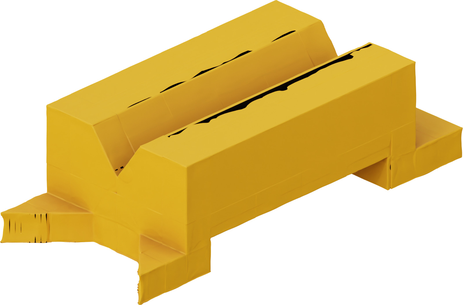
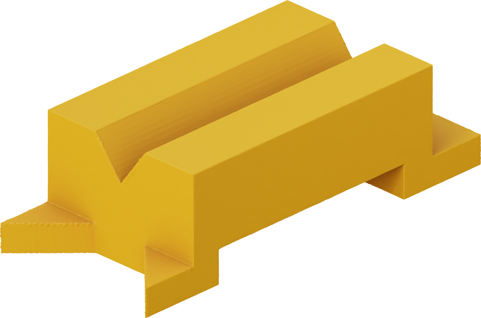
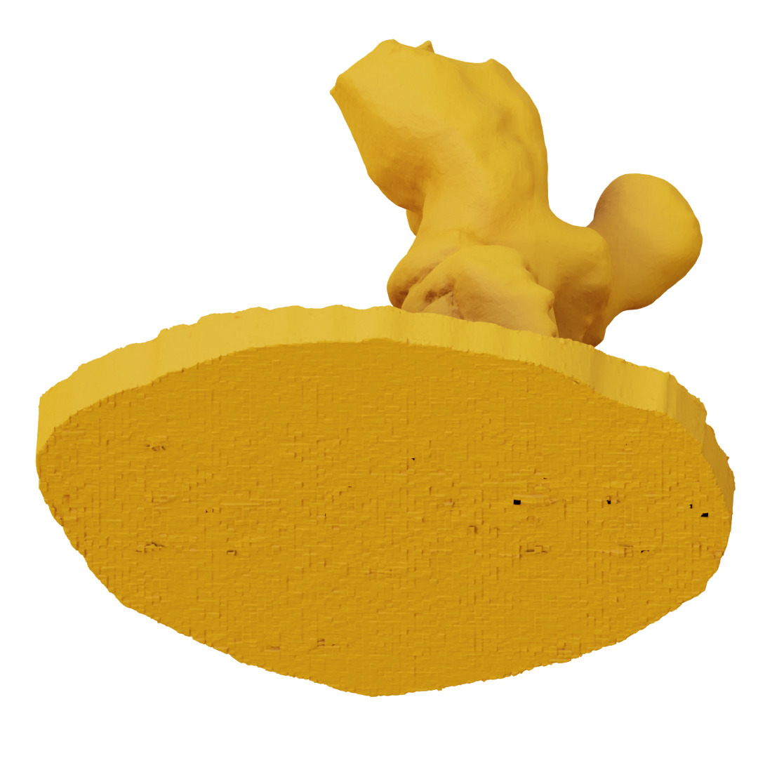
We provide some general visualization cases of the limitations of our method and regular grids with SDFs. Due to the normal alignment of our octree and the developed interpolation scheme, the oriented-grid encoder still outperforms the regular grid one. Since both methods have the same type of decoder, similar problems arise. However, our architecture mitigates some of those issues. Fig. C.14 shows fewer holes and more robustness for thinner surfaces for oriented grids, which can also be seen for occupancy output in Fig. 6 in the main paper.
C.4 Additional Matterport3D scenes
We show two additional scenes from Matterport3D with oriented grids in Fig. C.16. The proposed encoder can reliably obtain high detail in challenging scenes with thin surfaces and complex environments.