Simba-EoR: Early galaxy formation in the Simba simulation including a new sub-grid interstellar medium model

Abstract

We update the dust model present within the Simba galaxy simulations with a self-consistent framework for the co-evolution of dust and molecular hydrogen populations in the interstellar medium, and use this to explore $z\geq 6$ galaxy evolution. In addition to tracking the evolution of dust and molecular hydrogen abundances, our model fully integrates these species into the Simba simulation, explicitly modelling their impact on physical processes such as star formation and cooling through the inclusion of a novel two-phase sub-grid model for interstellar gas. In running two high-resolution simulations down to $z\sim 6$ we find that our Simba-EoR model displays a generally tighter concordance with observational data than fiducial Simba. Additionally we observe that our Simba-EoR models increase star formation activity at early epochs, producing larger dust-to-gas ratios consequently. Finally, we discover a significant population of hot dust at $\sim 100$ K, aligning with contemporaneous observations of high-redshift dusty galaxies, alongside the large $\sim 20$ K population typically identified.

1 Introduction

The James Webb Space Telescope (JWST), launched in late 2021, boasts the capability to run astrophysical surveys groundbreaking in their width, depth and accuracy (Gardner et al., 2006). Relevant to this study, JWST will observe galaxies at redshifts $z>6$, collecting state-of-the-art datasets applicable to the research of galaxy formation and evolution. Observable properties taken from JWST images will enable us to quantify parameters critical for a galaxy’s evolution, such as its star formation rate (SFR), dust-to-gas ratio, hydrogen abundance and metallicity; giving physical insight into the galactic environment as observed, in addition to its past and future evolution. Furthermore, as the unprecedented depth of JWST observations allows us to probe further into our universe’s past with greater accuracy than ever before, it is now possible to observe the evolution of galactic structure during the epoch of reionisation with statistical rigour never-before-seen.

Analysing and interpreting these high-redshift JWST datasets requires a more sophisticated understanding of the theory behind galaxy formation during the epoch of reionisation than we currently have. To this end, large-scale cosmological simulations consisting of many physical models are employed with the goal of producing datasets concurrent with observation; thereby facilitating the experimentation and validation of theoretical models which are impracticable to test in the real-world. Currently there exist many simulation suites which are generally successful in reproducing a variety of observed galaxy properties; though each have their own specialities and limitations. Examples of such codes active in the modern climate include: EAGLE (Schaye et al., 2015), THESAN (Kannan et al., 2022), ILLUSTRIS-TNG (Pillepich et al., 2018), and Simba (Davé et al., 2019). Suites such as these are typically built from pre-existing physical simulation codes, improving upon specific aspects in the modelling and calculation schemes to target research into certain physical phenomena.

Computationally there exists a range of simulation architectures, each optimal for the investigation of different astrophysical scenarios. For example ENZO (Collaboration et al., 2014) is a grid-based code wherein the coordinate space is broken into a matrix of cells; each representing the physical conditions of the gas (alternatively the cell can represent the containing dark matter, stellar population or any other relevant field) contained within it. GADGET-4 (Springel et al., 2021) and GIZMO (Hopkins & Raives, 2016) are popular choices when it comes to running simulations using the smoothed particle hydrodynamics (SPH) framework. Instead of dividing space into a grid and evaluating the physical fields within each cell, SPH populates the coordinate space with a number of particles which interact with their neighbouring particles within some smoothing radius. These fundamentally different approaches (along with many others we fail to mention in this introduction) each have their own use cases in regards to which physical scenario they are best suited. For example, SPH simulations are less well suited to reproduce phenomena such as dynamical instabilities (Agertz et al., 2007) when compared to mesh-based codes, but perform better in scenarios where the density fluctuates considerably between regions (Bate & Burkert, 1997).

Simba, takes advantage of GIZMO’s SPH solver to run its simulations, whilst adding sophisticated sub-grid modelling for physical mechanisms such as black hole feedback and stellar winds (Davé et al., 2019; Hopkins & Raives, 2016). These sub-grid models are necessary to include physical phenomena which occur on scales smaller than the resolution limit of the simulation itself. For example, star formation, which is triggered by the collapse of gas within giant molecular clouds (GMCs) to high densities $\sim 10^{6}\,\,\mathrm{cm}^{-3}$ is left unresolved in typical modern cosmological simulations. Therefore, to include star formation it must be modelled as a function of particle quantities (density, metallicity etc.) in addition to sub-grid parameters which are tuned such that the model reproduces observation. In the case of Simba, a sub-grid model in which the star formation rate (SFR) is proportional to both the density and molecular hydrogen fraction of the gas is implemented. Moreover, the fraction of molecular hydrogen is calculated sub-grid through use of the Krumholz-McKee-Tumlinson (KMT) model, which assumes a spherical cloud of gas irradiated by a uniform isotropic dissociating radiation field under idealised conditions (Krumholz et al., 2009; Krumholz, 2014). This results in the molecular hydrogen fraction being dependent on only two gas quantities: its metallicity and dust column density.

The growth and destruction of galactic dust is also tracked sub-grid in Simba (using the model proposed in Li et al. 2019) where the dust population can grow through accretion of gas-phase metals and shrink as a result of supernovae shocks and thermal sputtering. Though this model is fully implemented in the simulation, there exists (prior to this work) no communication between itself and the molecular hydrogen model: which one might expect due to the dust’s role in catalysing the primary H₂-forming chemical reaction. Furthermore, this model contains many free ‘reference’ parameters, some of which are theoretically obsolete in the context of a simulation of higher sophistication.

The aim of our work is to marry the modelling of star formation, molecular hydrogen and galactic dust in a self-consistent network through which they are inter-dependent as motivated from theory. We achieve this by first increasing the capacity of our chemical network such that it tracks explicitly the formation of molecular hydrogen both in the presence and absence of dust. Next, we remove the KMT model, replacing it with the chemically-motivated H₂ fraction and introducing a new sub-grid model for the interstellar medium (ISM). Furthermore, we introduce a calculation of the local interstellar radiation field (ISRF) incident on each particle, which is used to compute the dust temperature. Lastly, we replace the dust model’s reference temperature ($20$ K) with the dust temperature calculated explicitly for each particle, thereby modifying the rate at which the dust population evolves and as such the molecular hydrogen fraction.

It is important to note that the KMT model approximates the strength of dust shielding via the metal surface density. We know that this is not entirely accurate because in reality the dust-to-metal ratio is not constant, which warrants an improved treatment of dust shielding. However, Grackle does not currently possess the functionality to compute dust shielding, and as such this mechanism is omitted in our study. Possible avenues for future work on this are to include an attenuation to the ISRF based on the amount of dust present, or implement a full radiative transfer approach.

In Section 2 we provide technical descriptions of the calculations used in our models, providing physical explanation where appropriate. Furthermore, we also detail the practical facets of our simulation including the procedures employed in testing and verification. Section 3 offers comparison between our Simba-EoR simulations, those of fiducial Simba, and practical observations. In Section 4 we carry out a post-processing procedure on population of galactic particles to quantify the difference between our explicit calculations of the molecular hydrogen fraction ($f_{\mathrm{H}_{2}}$) using our ISM model, and the KMT-estimated values. Our final set of results are presented in Section 5 where we investigate the thermodynamic state of the dust and cool-phase ISM gas present in our simulations. Finally, Section 6 provides a summary of our findings alongside proposals for future work.

2 Methods

We run the Simba (Davé et al., 2019) simulation with updated, self-consistent modelling for dust, molecular hydrogen and star formation; achieved through implementation of Grackle’s (Smith et al., 2017) nine-species chemical network and dust thermodynamics. Our simulations consisted of $1024^{3}$ gas and 1024³ dark matter (DM) particles inside periodic boxes of side-length 50 Mpc/h and 25 Mpc/h, both with a cosmology of $\Omega_{m}=0.3$, $\Omega_{\Lambda}=0.7$, $\Omega_{b}=0.048$, $H_{0}=68$ km s^-1 Mpc^-1, and $\sigma_{8}=0.82$. The runs began at $z=249$ and were evolved down to $z=6$, producing a total of 36 snapshots during their evolution.

2.1 Star Formation in Simba

Simba implements a stochastic, H₂-driven star formation procedure (Davé et al., 2016, 2019) where, prior to the integration of Grackle’s molecular network, the abundance of molecular hydrogen was described by Krumholz, McKee & Tumlinson’s model – henceforth referred to as the KMT model (Krumholz et al., 2009; Krumholz & Gnedin, 2011). The major advantage of this prescription is its low computational cost and simple, two-parameter dependence on the column density and metallicity; both of which are easily calculated during run-time. Whilst this is an appropriate model to use in such simulations, its degree of straightforwardness requires the pretext of many assumptions regarding the gaseous cloud and its environment: we remove such assumptions by explicitly tracking the molecular hydrogen abundance using Grackle (Smith et al., 2017) as explained in Section 2.6.

The star formation rate for a gaseous SPH particle is given by,

$$\frac{dM_{\star}}{dt}=\epsilon_{\star}\frac{\rho f_{\text{H}_{2}}}{t_{\text{dyn}}}$$ (1)

where $\epsilon_{\star}=0.02$ is the star formation efficiency, $f_{\text{H}_{2}}$ is the molecular hydrogen fraction of the particle, and $t_{\text{dyn}}$ is the dynamical time (the time taken for a homogeneous, spherical gas cloud to collapse in free-fall). Stars are formed in a probabilistic fashion, the likelihood of which primarily depends upon the gas particle’s SFR, duration of the current time-step and total gas mass present.

2.2 Two-Phase ISM Model

In order to update the star formation model (see Section 2.1), we replaced the KMT model’s estimates with the molecular hydrogen fraction as calculated from the chemical network directly. However, as the densities required for star formation are beyond the resolution limits of our cosmological simulations, we introduced a two-phase, sub-grid model for gas in the interstellar medium wherein we model sufficiently dense clouds as being composed of both a warm (low-density) and cool (high-density) phase (Springel & Hernquist, 2003).

By default, gas particles represent a population of hot gas at relatively low density. However, once the gas is thought to be capable of forming stars ($\rho>0.2\,\,\,n_{\text{H}}\,\text{cm}^{-3}$ in our case) we activate an additional phase within the particle, that of the cool, dense gas from which stars are formed. In practice, this activation is carried out through tracking an additional density and energy field, and assuming that each phase contains half the total mass of the original particle. We allow ISM particles (by which we refer to those with both phases active) to revert to ‘standard’ gas particles if they are no longer potentially star-forming. Each simulation timestep, we update the cool phase density such that it maintains pressure balance with the warm phase, whose properties are in turn updated by the hydrodynamical solver. This pressure balance is expressed mathematically as,

$$\rho_{\text{cool}}U_{\text{cool}}=\rho_{\text{warm}}U_{\text{warm}}$$ (2)

where $U$ is the internal energy. It is important to note that in the two-phase regime, only the cool phase is explicitly cooled due to its relevance for star formation. The warm phase, the temperature of which is held at $10^{4}$ K from the equation of state, is used for all other aspects of the simulation such as the hydrodynamic fluid solver. This approach enhances the density of the ISM sufficiently to form stars at rates comparable with the KMT model we replaced, whilst maintaining the self-consistency and accuracy of an explicit chemical network.

It should be noted that as we model star formation stochastically, (see Section 2.1) it is possible that a given gas particle will cool and collapse far beyond the threshold density for star formation, potentially reaching much larger densities before forming a star particle.

2.3 Dust Temperature

The significance of dust in galaxy formation and evolution is not to be understated. The presence of dust grains in the galactic environment acts as a catalyst for molecular formation, namely H₂, which is critical for cooling and star formation. Additionally, grains contribute to the thermodynamic state of the system whether that be through: heat exchange with the gas; heating from incident radiation fields, or cooling via thermal emission.

2.3.1 Grackle’s Solver

We employ Grackle (Smith et al., 2017) to handle the calculation of the dust temperature; accomplished by using Newton’s method to solve the heat balance equation,

$$4\sigma T_{\text{gr}}^{4}\kappa_{\text{gr}}=4\sigma T_{\text{rad}}^{4}\kappa_{\text{gr}}+\Lambda_{\text{gas-grain}}$$ (3)

where $\sigma$ is the Stefan-Boltzmann constant, $T_{\text{gr}}$ and $T_{\text{rad}}$ are the temperatures of the dust grains and incident radiation field respectively, $\kappa_{\text{gr}}$ is the grain opacity, and $\Lambda_{\text{gas-grain}}$ is the rate of heat transfer between the gas and dust per unit grain mass. The left-hand and right-hand sides of Equation 3 describe the cooling and heating contributions respectively. As discussed in Hollenbach & McKee (1989), the gas-grain term is a function of both the gas and grain temperatures. Specifically,

$$\Lambda_{\text{gas-grain}}\propto\left(T_{\text{g}}-T_{\text{gr}}\right)$$ (4)

where $T_{\text{g}}$ is the gas temperature. From this definition, it can be deduced that when $\Lambda_{\text{gas-grain}}>0$, the dust is being heated by the gas, hence its appearance on the right-hand side in Equation 3.

The opacity of a grain is modelled as a function of its temperature, as presented in Dopcke et al. 2011,

$$\kappa_{\mathrm{gr}} \propto\begin{cases}T_{\mathrm{gr}}^{2};&T_{\mathrm{gr}}<200\,\,\mathrm{K}\\ \mathrm{constant};&200\,\,\mathrm{K}<T_{\mathrm{gr}}<1500\,\,\mathrm{K}\\ T_{\mathrm{gr}}^{-12};&T_{\mathrm{gr}}>1500\,\,\mathrm{K}\end{cases}$$ (5)

where we normalise $\kappa_{\mathrm{gr}}=16\,\,\mathrm{cm}^{2}\,\mathrm{g}^{-1}$ at $T_{\mathrm{gr}}=200\,\,\mathrm{K}$ (Smith et al., 2017). The constant regime at intermediate temperatures models the evaporation of the grain’s icy mantle, whilst the steep power law at extreme temperatures accounts for dust sublimation (Dopcke et al., 2011).

2.3.2 Inclusion of an External Radiation Field

By default, $T_{\text{rad}}$ in Equation 3 consists solely of contributions from Cosmic Microwave Background (CMB) radiation. As discussed in Section 2.4, the ISRF is computed at simulation run-time for each particle from characteristics of its local galactic environment. Therefore, $T_{\text{rad}}$ should incorporate this to improve the calculation of $T_{\text{gr}}$.

Preexisting functionality within Grackle allows us to provide an ISRF by including an additional term in Equation 3 such that it becomes,

$$4\sigma T_{\text{gr}}^{4}\kappa_{\text{gr}}=4\sigma T_{\text{rad}}^{4}\kappa_{\text{gr}}+\Lambda_{\text{gas-grain}}+\Gamma_{\text{ISRF}}G_{0}$$ (6)

where $G_{0}$ is the ISRF field strength in Habing units and $\Gamma_{\text{ISRF}}$ is the dust heating rate resultant from the ISRF (Habing, 1968; Krumholz, 2014). The addition of this term circumvents the need to modify $T_{\text{rad}}$ directly, and allows us to pass our calculated ISRF to Grackle easily.

2.4 Modelling the ISRF

The strength of the ISRF is an important and significant parameter in many astrochemical calculations, namely the species’ abundances within the galactic environment. In our case, to compute the dust temperature, the local ISRF strength is a necessary input and therefore must be calculated at run-time. This is a non-trivial exercise, as the variables required for its direct computation (e.g. stellar luminosity) are not tracked during the simulation.

A typical approach to this problem is to use an external code such as STARBURST99 (Leitherer et al., 1999) which is able to generate estimates of the luminosity for a range of input parameters; notably the initial mass function (IMF), stellar age and metallicity. By interpolating over a grid of suitable parameter values, a lookup table for the luminosity can be created and later referenced during simulation run-time. Calculation of the ISRF using this estimate is then straight forward, for example, employed in Olsen et al. (2017) is,

$$G_{0}=\sum_{\rvert\vec{r}_{\text{gas}}-\vec{r}_{\star,i}\rvert<h}\frac{L_{\star}}{4\pi\rvert\vec{r}_{\text{gas}}-\vec{r}_{\star,i}\rvert^{2}}\frac{M_{\star}}{10^{4}M_{\odot}}$$ (7)

where $L_{\star}$ is the stellar luminosity, $\rvert\vec{r}_{\text{gas}}-\vec{r}_{\star,i}\rvert$ is the separation between the target gas particle and stellar source, $M_{\star}$ is the stellar mass of the source.

Instead of using a pre-computed method such as that described above, we implemented an on-the-fly scheme to calculate the ISRF incident upon a given gas particle; allowing us to account for the state of the local stellar environment at the current time-step.

We model the ISRF as being proportional to the specific star formation rate (sSFR), where the proportionality is assumed to be that of the Milky-Way,

$$G_{0,i}=\frac{G_{0,\text{MW}}}{\mathrm{sSFR}_{\mathrm{MW}}}\mathrm{sSFR}_{i}$$ (8)

where $i$ and MW denote the target particle and Milky-Way respectively (Olsen et al., 2017; Licquia & Newman, 2015). The total sSFR within the target particle’s local environment is denoted sSFR_i and is the term calculated at run-time.

We calculate $\mathrm{sSFR}_{i}$ as a kernel-weighted average of the specific star formation rates present within one smoothing length of the target particle. Furthermore, we smooth this field to alleviate any unphysical boundaries which could manifest due to the geometric configuration of particles. For example, consider the case where the target particle has an average sSFR calculated much smaller than that of another particle just outside of its smoothing kernel. In this scenario, physically, the target particle’s sSFR should have a significant contribution from this external particle, but due to the nature of the calculation this is not considered. Therefore, after the calculation for the target particle, we take a kernel-weighted mean of the total sSFR’s of all particles within its smoothing kernel. This smoothed value corresponds to $\dot{M}_{\text{sSFR},i}$ in Equation 8.

To prevent the occurrence of a systematic smoothing bias in our calculations (specifically, an aggregate affect where particles calculated later in a given time-step will be more smoothed than those at the beginning) we only allow the pre-smoothed values of a particle’s neighbours to be used in the calculation. This ensures the ‘degree-of-smoothing’ for every particle in our simulation is constant. Lastly, please note that in its current form this model does not include any ISRF attenuation which may arise due to interaction with the ISM through which it propagates.

2.5 Dust Growth and Destruction

Having implemented models for both the local, incident ISRF and dust temperature of a given particle, the final step is to include the modelling of dust. Originally published in Li et al. (2019), this models describes the growth of dust grains via metal accretion, and their destruction as a result of supernovae and thermal sputtering.

2.5.1 Metal Accretion

Dust grains grow in size through the accretion of gaseous metals, the rate of which is given by,

$$\left(\frac{dM_{\text{gr}}}{dt}\right)_{\text{growth}}=\left(1-\frac{M_{\text{gr}}}{M_{\text{met}}}\right)\frac{M_{\text{gr}}}{\tau_{\text{accr}}}$$ (9)

where $M_{\text{gr}}$ is the dust grain mass, $M_{\text{met}}$ is the total metal mass in both the gaseous and dust phases Dwek (1998). Furthermore, $\tau_{\text{accr}}$, the accretion timescale takes the form,

$$\tau_{\text{accr}}=\tau_{\text{ref}}\left(\frac{T_{\text{ref}}}{T_{\text{g}}}\right)^{1/2}\left(\frac{\rho_{\text{ref}}}{\rho_{\text{g}}}\right)\left(\frac{Z_{\odot}}{Z_{\text{g}}}\right)$$ (10)

where $\tau_{\text{ref}}$, $Z_{\odot}$ and $\rho_{\text{ref}}$ are the reference timescale, solar metallicity and density respectively; analogous variables for the gas are subscripted ‘g’ (Li et al., 2019; Asano et al., 2013; Hirashita, 2000). These constants are set to the following values in this work:

$$\tau_{\text{ref}} =0.4\,\,\,\,\text{Myr}$$

$$\rho_{\text{ref}} =2.3\times 10^{-22}\,\,\,\,\text{g}\,\text{cm}^{-3}$$

$$Z_{\odot} =0.01295$$

It may be useful to note that $\rho_{\text{ref}}\sim 100\,\,\text{n}_{\text{H}}\,\text{cm}^{-3}$, and the solar metallicity value originates from Cloudy (version 13) Ferland et al. (2013). Although the choice of these values is somewhat arbitrary, they have been chosen to represent the ‘common’ physical scenario.

There is one key difference in our model versus the Li et al. (2019) model – we replace the reference temperature ($T_{\mathrm{ref}}$ = 20 $\mathrm{K}$ originally) with the dust temperature. This is done as a crude representation of the dust temperature’s influence on the accretion rate; specifically the sticking potential of metals onto grains (Hirashita & Kuo, 2011; Spitzer, 2004). The exact form of the sticking potential is difficult to obtain with its many complex dependencies on the chemical composition of the grains in addition to the environment in which they preside (Jones & Nuth, 2011). As our model does not attempt to represent the distribution of grain sizes, nor their chemical composition, integrating an accurate sticking potential is impracticable in this work. Furthermore, we must be careful to retain the characteristics of the original model, altering the accretion rate’s temperature dependence too much would constitute a new model itself and is not the aim of this work. We re-tune $\tau_{\mathrm{ref}}$ such that our model aligns with expected results for the stellar mass function at redshift 6. Exact details of these changes are presented in Appendix A, alongside a derivation of Equation 10.

It bears clarification that this model assumes a constant radius of $0.1\,\,\mu\mathrm{m}$ for all dust grains, omitting the inclusion of a grain size distribution. Thus, when dust grains grow/shrink in our model, we are referring to a change in their mass and metallicity; their cross-section (relevant in the formation of molecular hydrogen, see Section 2.6.2) remains constant. Models which account for the distribution of grain sizes are a current area of interest, and such future enhancements will make for an appreciable update to our model. We refer the curious reader to Romano et al. 2022, where both molecular hydrogen and dust are modelled using a distribution of grain sizes.

2.5.2 Dust Sputtering

Thermal sputtering is the process by which dust grains moving within a hot gas are abraded due to the collisions between the dust and gas phases: a result of the gas’ high temperature (Draine & Salpeter, 1979; Tielens et al., 1994). The sputtering timescale is defined as $\tau_{\text{sput}}=a/\left|\dot{a}\right|$, where $a$ is the grain radius. This can be approximated as a function of the gas density and temperature in addition to the grain size: for a comprehensive discussion of this please see Tsai & Mathews (1995) and Li et al. (2019). Then, the rate at which dust grains grow due to sputtering is given by,

$$\left(\frac{dM_{\text{gr}}}{dt}\right)_{\text{sput}}=-\frac{M_{\text{gr}}}{\tau_{\text{sput}}/3}.$$ (11)

2.5.3 Destruction via Shocks

Thermal sputtering of dust (see Section 2.5.2), whilst able to completely destroy small grains through continued erosion, is not sufficient for larger grains. The destruction of these large grains is primarily driven by shocks originating from supernova remnants, SNRs, (Slavin et al., 2015). The timescale for this destruction is given by,

$$\tau_{\text{de}}=\frac{M_{\text{g}}}{\epsilon\gamma M_{\text{s}}}$$ (12)

where $\epsilon=0.3$ is the grain destruction efficiency from Type-II Supernovae, SNII, (McKee, 1989), $\gamma$ is the rate at which SNII occur in the local environment, and $M_{\text{s}}$ is the mass of the shocked gas, per supernova, travelling at $100\,\,\text{km}\,\text{s}^{-1}$ or faster. It is assumed in these definitions that SNI (Type-I supernovae) are negligible relative to SNII due to the particular circumstances under which they occur, and their subsequent low explosion frequency. In practice, the SNII rate is passed to the model from the simulation itself, whilst the mass of shocked gas is calculated using the Sedov-Taylor approximation.

2.6 The Abundance of Molecular Hydrogen

The abundance of molecular hydrogen within the ISM is largely dependent upon the amount of dust present. In the absence of dust, molecular hydrogen struggles to form efficiently due to its nucleic symmetry and subsequent lack of dipole transition. Upon the collision of two neutral hydrogen atoms, in the case that they bond to form H₂, their excess kinetic energy will cause the molecule to exist in an unstable state. Unless this excess energy is radiated from the molecule, it will dissociate and the constituent atoms will separate. Due to the absence of dipole transition, H₂ must radiate via forbidden magnetic quadrupole transition. The lowest-lying transition of this type has a transition probability of $\sim 10^{-11}\,\,\text{s}^{-1}$, which is far too unlikely to occur within the lifetime of the unstable molecule (Bromm, 2013).

Nevertheless, there are chemical pathways through which molecular hydrogen can form in the absence of dust (such as in the primordial case), although they are much slower. A brief discussion of both scenarios alongside their implementations will be presented below due to the novel nature of their inclusion within Simba (see Section 2.1).

2.6.1 The Primordial Case

In the primordial gas there exist three primary channels through which molecular hydrogen forms (Galli & Palla, 1998); the first of which we will consider being the following,

$$\text{H}+\text{e}^{-}\longrightarrow\text{H}^{-}+\gamma$$

$$\text{H}^{-}+\text{H}\longrightarrow\text{H}_{2}+\text{e}^{-}$$

wherein a free electron associates with a neutral hydrogen atom, creating H^-, which is stable due to its permanent electric dipole and resultant radiative transition. This proceeds form H₂ upon collision with another neutral hydrogen atom, which forms a stable molecule due to the ejection of the free electron which carries any excess energy; therefore removing the need for fast radiative emission. As the first reaction above requires collision with a free electron, the ionisation factor of the gas is primary in determining the effectiveness of this pathway.

At high redshifts, $z\gtrsim 100$, photons from the cosmic microwave background (CMB) are sufficiently energetic to dissociate the weakly-bound H^- species necessary in the formation channel above. However, these photons are unable to destroy H${}_{2}^{+}$ and so we consider the second pathway,

$$\text{H}^{+}+\text{H}\longrightarrow\text{H}_{2}^{+}+\gamma$$

$$\text{H}_{2}^{+}+\text{H}\longrightarrow\text{H}_{2}+\text{H}^{+}$$

where the ejection of a proton removes any excess energy from the newly formed molecule. This channel is significantly slower than the first and as such is only important in the regime under which the first cannot operate (Bromm, 2013; Tegmark et al., 1997).

The final pathway we will detail here is that of the three-body reaction,

$$\text{H}+\text{H}+\text{H}\longrightarrow\text{H}_{2}+\text{H}$$

which only becomes effective at high densities ($n\gtrsim 10^{8}\,\,\mathrm{cm}^{-3}$) where the rate at which three-body collisions occur is non-negligible. Furthermore, as the density of the gas increases, so too does the rate of ion-electron recombination – ultimately reducing the density of free electrons in the gas and therefore the rate of H₂ formation in the first channel Turk et al. (2011b).

2.6.2 In the Presence of Dust

Dust grains are the primary channel through which molecular hydrogen is formed within the collapsing gaseous cloud described above. The grains present within a dust-enriched cloud are sites of active H₂ formation due to their ability to capture hydrogen atoms on their surface, absorbing the atom’s kinetic energy upon collision. Over time, a large population of hydrogen atoms will accumulate on the surface of a grain. Able to move slowly on the grain surface, these atoms will collide with one-another to form H₂. Excess energy which threatens to destabilise the molecule will be used to overcome the sticking potential of the grain, allowing the hydrogen molecule to leave the grain surface and re-enter the gas phase.

The dust-catalysed H₂ formation rate, as prescribed in Tielens & Hollenbach (1985), can be expressed as,

$$R=\frac{1}{2}\overline{v}_{\text{H}}n_{\text{H}}n_{\text{gr}}\sigma_{\text{gr}}\epsilon_{\text{H}_{2}}S(T)\,\,\,\,\text{cm}^{-3}\,\text{s}^{-1}$$ (13)

where $\overline{v}_{\text{H}}$, $n_{\text{H}}$, $n_{\text{gr}}$, $\sigma_{\text{gr}}$, $\epsilon_{\text{H}_{2}}$ and $S(T)$ are the average velocity and number density of hydrogen atoms, number density of dust grains, grain cross-section, efficiency of grain-bound molecular hydrogen formation and the sticking coefficient of hydrogen atoms respectively (Schneider et al., 2006). Due to the complex dependencies present in Equation 13 we employ the following approximation shown in Hollenbach & McKee (1989),

$$R\simeq 6.39\times 10^{-15}\left(\frac{T}{300}\right)^{1/2}n_{\text{gr}}n_{\text{H}}S(T,T_{\mathrm{gr}})\,\,\,\,\text{cm}^{-3}\,\text{s}^{-1}$$ (14)

The sticking coefficient describes how readily hydrogen atoms will be become bound to the grain surface and is thus dependent on both the gas and grain temperatures as detailed in Hollenbach & McKee (1979),

$$S(T,T_{\mathrm{gr}})=\left[1+0.4\left(\frac{T+T_{\text{gr}}}{100\,\text{K}}\right)^{1/2}+0.2\left(\frac{T}{100\,\text{K}}\right)+0.08\left(\frac{T}{100\,\text{K}}\right)^{2}\right]^{-1}.$$ (15)

3 Comparison with Observation and Fiducial Simba

In this section we offer comparison between observed results, Simba’s fiducial modelling prescription, and the new models presented in this work. We include both simulation sizes: the larger box of side-length 50 Mpc/h containing 2 $\times$ 1024³ particles (baryonic and dark matter); and the smaller 25 Mpc/h box with the same number of particles, resulting in a simulation with 8$\times$ higher mass resolution. These runs are labelled ’m50n1024’ and ’m25n1024’ respectively. All results presented in this section are taken from the redshift 6 snapshot unless explicitly stated otherwise.

3.1 Mass Functions

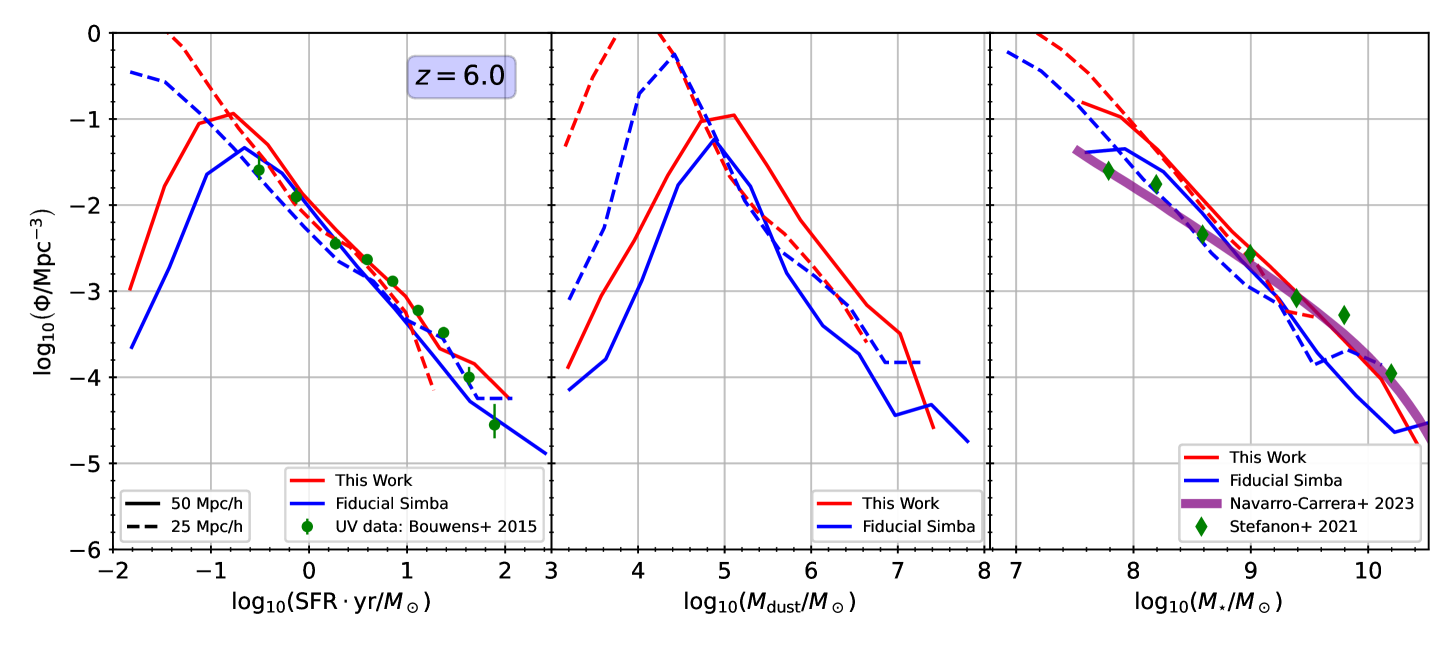
Figure 1: The mass functions for the star formation rate (left), dust mass (centre) and stellar mass (right) at redshift 6. The blue and red lines show results from fiducial Simba and this work’s runs respectively. Further, solid/dashed lines differentiate between the 50/25 Mpc/h simulations. Left: We add the UV data presented in Bouwens et al. 2015 for comparison with our simulations and see a high level of agreement between all for $\mathrm{SFR}\gtrsim 10^{-1}\,\,M_{\odot}/\mathrm{yr}$. At low star formation rates we see considerable divergence with resolution. Centre: We observe similar trends as were seen for the SFR; the box-sizes diverging significantly at $M_{\mathrm{dust}}\lesssim 10^{4.8}\,\,M_{\odot}$. It is expected that there is a tight correlation between SFR and dust mass due to its importance in the cooling of star-forming regions. Right: Data from Navarro-Carrera et al. 2023 and Stefanon et al. 2021 is plotted alongside the simulation results to show their physicality. Tight agreement between the data and simulations is seen at larger stellar masses, whilst the simulations overestimate the data at low stellar mass. For each resolution it can be seen that our models produce more stellar mass than fiducial Simba across the domain.

In Figure 1 we plot the SFR (left panel), dust mass (centre panel) and stellar mass (right panel) functions for galaxies identified in both our simulations (red) and the fiducial Simba runs (blue). The size of the simulation box is displayed by solid and dashed lines for the 50 and 25 Mpc/h runs respectively. Where appropriate, observational results have been added to serve as a reference for comparison between datasets. Observing the three panels we identify some general trends: our models predict larger number densities than their fiducial counterparts; the high-resolution boxes contain significantly more data at the lowest values; all four simulations display a high level of agreement throughout the intermediate-high values; and all simulated datasets effectively reproduce observational results.

The divergence at low values arises purely due to numerical resolution; the higher resolution volume is able to resolve smaller systems. On the other hand, one can also see that the larger volume tends to have higher number densities at the very highest values. This is because the smaller volume is less able to produce a representative sample of the most mass massive systems. Therefore the most robust predictions are in the intermediate galaxy size range, and we will focus our discussion there.

The leftmost panel describes the distribution of star formation rates produced by the simulations, in addition to observational UV results from Bouwens et al. (2015) for comparison. Here, it appears that robust predictions arise with the range of $10^{-0.6}\,\,M_{\odot}/\mathrm{yr}\lesssim\mathrm{SFR}\lesssim 10^{1.2}\,\,M_{\odot}/\mathrm{yr}$, which is resolved in both simulations but is not so large as to be subject to stochasticity due to the finite volume. Within this range, we see the slope and amplitude of the observational SFR function is broadly well-reproduced by all the simulations. Also, there is generally good concordance between the predictions of the two volumes, suggesting that the SFR function is reasonably well resolution-converged.

That said, closer inspection reveals that within the robustly predicted range, the Simba-EoR simulations (red) yield somewhat better agreement with the observations as compared to the Simba runs (blue). Simba tends to produce a steeper slope than observed, and insufficient high-SFR galaxies. This is important because Simba has difficulty reproducing the very brightest early galaxies (Finkelstein et al., 2023), and this suggests that Simba-EoR may do a bit better; we will explore this further when we compare directly to UV luminosity functions next. Also, for both models, the 25 Mpc/h runs tends to predict values that are $\sim 0.1$ dex lower than the 50 Mpc/h runs, indicating a slight level of non-convergence even within the well-resolved regime.

The dust mass function (shown in the centre panel) is seen to have somewhat different trends to the SFR function. Firstly, we identify robust predictions within the range of $10^{4.8}\lesssim M_{\mathrm{dust}}\lesssim 10^{6.6}\,\,M_{\odot}$, where all runs appear to give resolved predictions. Here, we see larger discrepancies between the new Simba-EoR predictions and Simba, at least for the 50 Mpc/h run. Interestingly, the smaller volume shows substantially less differences; it is not entirely clear why. Neither volume is all that well resolution-converged, but in different senses: Simba-EoR’s larger volume produces more dust, while Simba’s produces less. Given the complex interplay between the dust model, star formation, metallicity growth, and other physical processes, it is not straightforward to interpret these trends. However, it is clear that all the models produce significant masses of dust in the early Universe. Therefore it will be important to account for dust extinction when examining forward-modelled properties in the observational plane.

The galactic stellar mass function, shown in the right-hand panel, offers robust predictions in the range $10^{7.8}\lesssim M_{\star}\lesssim 10^{9.8}\,\,M_{\odot}$ where the simulations are resolved. We see that all simulated runs, Simba and Simba-EoR, exhibit steeper gradients than the data of Navarro-Carrera et al. 2023 and Stefanon et al. 2021. Whilst all runs predict larger populations than observed at low stellar mass, as the stellar mass increases the computational models begin to under-predict this population. At larger stellar masses, $M_{\star}\sim 10^{9.6}\,\,M_{\odot}$ we good agreement between the Simba-EoR model and both observational datasets. Whilst the fiducial Simba model displays noticeable discrepancies between the 25 Mpc/h and 50 Mpc/h boxes across much of the resolved domain, the Simba-EoR boxes show good agreement, highlighting our model’s robustness. Furthermore, the Simba-EoR model contains more sources at each stellar mass than fiducial Simba, a reflection of its generally higher star formation rate as shown in the leftmost panel.

In summary, we see general agreement between the results of our model and the fiducial Simba model. Given that the fiducial model produced results which were physically viable itself, agreement with this is an ideal outcome for our model given its reduced parameterisation and self-consistent nature which removed the need for many assumptions previously used. The area where we see signs of our model offering improvement over its predecessor is around the resolution limit; though the impact of this is minimal.

3.2 The UV Luminosity Function

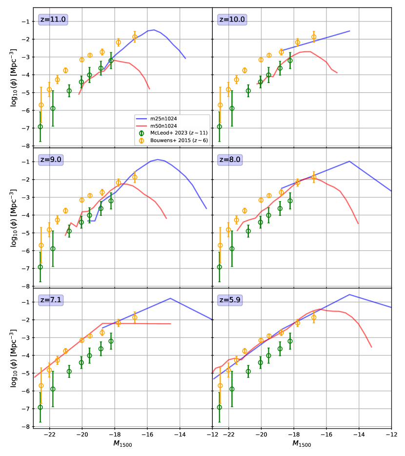
Figure 2: The UV luminosity function at varying redshift for both our 50 Mpc/h (red) and 25 Mpc/h (blue) boxes. Alongside, we include observational results from McLeod et al. 2023 (green) and Bouwens et al. 2015 (yellow): it is important to note that the former is taken from galaxies identified by JWST at redshift $\sim 11$ and as such we should expect some systematic offset compared to our results. At $z\sim 6$ we see that the brightest galaxies produced in our models are a considerably better fit to the data than fiducial Simba which under-produces bright sources.

The UV luminosity functions for the simulations presented in this work are shown in Figure 2. We differentiate between the simulated box-size using red lines for the 50 Mpc/h run and blue lines for 25 Mpc/h run. Furthermore, we add two observational datasets to our plot: the $z\sim 11$ JWST dataset of McLeod et al. 2023 in green, and the $z\sim 6$ dataset of Bouwens et al. 2015 (also present in Figure 1) in yellow. We plot the luminosity function from redshift $\sim 11$ to $\sim 6$ in integer steps to observe its temporal evolution. It should be noted that we have assumed a Milky-Way extinction law to produce the photometric data used in this paper.

To compute these UV magnitudes, a post-processed ray tracing procedure was ran using Pyloser, which calculates the dust extinction explicitly. This uses the dust properties of each particle as calculated in the simulation, meaning that the models implemented have a direct impact on the UV luminosity function. For example, if dust were ignored entirely, the UV luminosity function would show many more bright sources than the observational data. On the other hand, if the dust populations were overestimated (if grains grew too quickly for example) we would expect that the UV luminosity function would underestimate the number of bright sources.

First considering only the $z\sim 6$ function, we observe good agreement with the observational data at both simulated resolutions; our results capturing the luminosities of the brightest and dimmest observed sources well. Comparison between boxes shows that whilst the larger box exhibits a curvy, gradual turnover in its gradient throughout the magnitude range, the smaller box shows strong linear correlations with a sharp turnover at $\log_{10}(M_{1500})\approx-14.5$. This behaviour is caused by the difference in resolution between the two runs, similarly to that discussed above for the mass functions (Section 3.1).

Furthermore, the significantly larger abundance of dim sources in the smaller box (relative to the larger) is an expected resolution effect also. In the most extreme case, at $\log_{10}(M_{1500})\approx-13.2$, we see that the high-resolution box predicts number densities roughly $2.5$ orders-of-magnitude larger than its low-resolution counterpart. However, we see this resolution discrepancy is ameliorated as we move away from the resolution limit, from the dimmest to brightest sources, with the two boxes remaining coherent from $\log_{10}(M_{1500})\approx-16$ until $\log_{10}(M_{1500})\approx-23$.

Considering the gradient of our luminosity functions at each redshift, we see that both resolutions largely follow the slope of the closest (in redshift) observational dataset. At $z=11$ we see that the our 50 Mpc/h box follows the McLeod et al. 2023 datapoints closely until the resolution limit. Likewise the 25 Mpc/h box, though shifted towards the dimmer sources due to its higher resolution, is in 1-$\sigma$ agreement with the datapoints from McLeod et al. 2023 with which it shares a magnitude.

As the redshift decreases we see that, in general, the simulations shift towards the $z\sim 6$ datapoints of Bouwens et al. 2015. This is readily seen in the 50 Mpc/h box which is able to model the brighter sources observed in the datapoints more easily than the 25 Mpc/h box. Focusing on our 50 Mpc/h run, we see that at redshift 9, the dimmer end of our function is beginning to rise towards the low-redshift datapoints, which at redshift 8 is mirrored with the number density of bright sources increasing. By $z\sim 6$ we see that both boxes show good agreement with the data of (Bouwens et al., 2015), following the slope of the observations down to the brightest sources. The concordance of our simulations with the observed datapoints at redshifts 6 and 11 highlight our model’s aptitude in producing a physical population of luminous sources. This is a key aspect of further analysis such as the generation of mock spectra from our simulations.

In the wake of recent JWST observations at high redshift, it has been noted that high-redshift galaxies have considerably larger UV luminosities than previously thought (Dekel et al., 2023; Ferrara et al., 2023). We see that at redshift 11, our UV luminosity function agrees with recent JWST observations at the brightest resolved sources ($M_{1500}\simeq-20$) without our models making any specific consideration for this phenomena. If we compare the evolution of our UV luminosity function at its bright end, with the work presented in Ferrara et al. 2023 (Figure 4), we see that our models generally agree to within $\sim 0.5$ dex, though this is complicated by the limited resolution of our simulations at high redshift. We notice that our model under-predicts the source brightness at higher redshifts, and over-predicts those at lower redshifts, when compared to their model. However, as our model makes no consideration for the problem at hand, we believe the results to be in reasonable agreement overall.

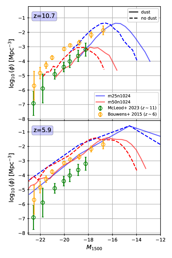
Figure 3: The UV luminosity function at redshift $\sim 10.5$ and $\sim 6$ for both our simulated boxes. We show the 50 Mpc/h and 25 Mpc/h runs in red and blue respectively, with observational data from McLeod et al. 2023 in green and Bouwens et al. 2015 in orange. Furthermore, we display the UV luminosity spectra as calculated from the absolute magnitude on straight lines, whilst that calculated from the absolute magnitude omitting the dust properties on dashed lines. We see that there exists a significant difference between the dust present/absent luminosity functions at both redshifts, with the dust-obscured samples containing fewer high-brightness sources than their dust-absent counterparts.

To understand the effect of dust on the UV luminosity function, we show in Figure 3, the dust-obscured (solid lines) and dust-absent (dashed lines) results at redshifts $\sim 10.5$ and $\sim 6$. As in Figure 2, the 50 Mpc/h and 25 Mpc/h runs are shown in red and blue respectively, with the orange and green data points representing observational data. At both redshifts, we observe an increase in the number density of bright sources (and complimentary decrease in dim sources) when the presence of dust is disregarded: as mentioned above, this is to be expected.

Crucially, this figure shows the significance of dust in the UV luminosity function, with the disparity between the dust-free and dusty cases manifesting distinctly in the plot. Thus, the subsequent agreement between our dust-attenuated luminosities and the observed datapoints suggest that our model possesses a degree of self-consistency; if the dust abundances calculated from our model were unreasonable, we would expect this to manifest as a clear divergence from the observed points on the plot.

3.3 The Time Evolution of the Star Formation Rate Density

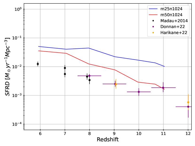
Figure 4: The SFRD’s evolution from redshift $\sim 11$ to $\sim 6$. Red and blue lines denote our 50 Mpc/h and 25 Mpc/h runs respectively, whilst points show data from Madau & Dickinson 2014 (black), Donnan et al. 2022 (purple) and Harikane et al. 2022 (orange). We see that whilst both of our simulations over-predict the SRFD consistently, the 50 Mpc/h run is a vastly better fit to the data than the 25 Mpc/h run.

Figure 4 shows the evolution of the star formation rate density (SFRD) with redshift. Our 50 Mpc/h and 25 Mpc/h runs are plotted as the red and blue lines respectively. The black, purple and orange points denote data taken from Madau & Dickinson 2014, Donnan et al. 2022 and Harikane et al. 2022 correspondingly. It is clear to see that in general, our simulations predict larger SFRDs than expected from the data across the entire redshift domain.

There exists, however, a striking difference between our simulations, with the 50 Mpc/h low-resolution run displaying a significantly closer fit to the data at high redshift than its 25 Mpc/h counterpart. Whilst both simulated boxes are in agreement to $\sim 0.2$ dex at redshift 6, at redshift 11 they displaying a disparity of $\sim 0.9$ dex; the larger box in 1$\sigma$ agreement with the recently observed data point of Donnan et al. 2022. We see that the 25 Mpc/h run’s SFRD-$z$ scaling has a far shallower gradient than that of the 50 Mpc/h run, resulting in the former’s significant disagreement with observed sources at high redshift.

Given the tension displayed here between both of our simulations, it is sensible to conclude the presence of some resolution dependency in the star formation mechanisms at high redshift. However, for future implementations of our model it is important to highlight the potential need for resolution-dependent tuning in the star formation models – none of which was carried out by us in the creation of this paper. Furthermore, simulations running to lower redshifts ($<6$) will require monitoring in this regard: our findings on our model’s low-redshift behaviour will be presented in a future paper.

3.4 The Mass-Metallicity Relation

Figure 5: The mass-metallicity relation observed in both the 50 Mpc/h (left panel) and 25 Mpc/h (right panel) simulation boxes. Red and blue lines depict linear, least-square fits to the results produced by the models presented in this work and fiducial Simba respectively. Additionally, results from Table 3 in Langeroodi et al. 2022 are plotted in green; these sources have spectroscopic redshifts in the range 7.2-8.5. Furthermore, the hexbin plot on each axis shows the distribution of galaxies found in our simulations, with darker shades corresponding to a higher count. Our models display more resolution dependence than the fiducial; the metallicity at fixed stellar mass increasing by $\sim 0.3$ dex in the high resolution box. Furthermore, the larger box shows considerably better agreement with the observational data plotted than its smaller counterpart.

Table 1: Results of the linear (in log-space) least-squares fits for the mass-metallicity relation presented in Figure 5.

Box-size (Mpc/h)	Model	Gradient	Intercept
50	This Work	$(2.13\pm 0.022)\times 10^{-1}$	$-2.8\pm 0.017$
50	Fiducial	$(3.9\pm 0.030)\times 10^{-1}$	$-4.3\pm 0.024$
25	This Work	$(2.1\pm 0.017)\times 10^{-1}$	$-2.5\pm 0.012$
25	Fiducial	$(3.2\pm 0.047)\times 10^{-1}$	$-3.7\pm 0.034$

In Figure 5 we plot show the mass-metallicity relation in the 50 Mpc/h and 25 Mpc/h boxes (left and right panels respectively) for both the simulations presented in this work and fiducial simba: these are shown in red and blue respectively. The plotted lines show a least-squares, linear fit (in log-space) to the underlying data, the results of which are detailed in Table 1. We also add a subset of the observational data presented in Table 3 of Langeroodi et al. 2022 as green points on the plot. We choose these points such that the observed sources have a spectroscopic redshift in the range $7.2\lesssim z\lesssim 8.5$. Lastly, we show the distribution of galaxies identified in our simulations on the hexbin in the background. This is shaded by the number of counts in each bin, with darker shades indicating a larger number of sources.

Comparing the two panels we immediately notice the shift toward higher metallicities introduced in our simulations upon increasing the resolution. In contrast to our 50 Mpc/h fit, which is seen to lie within within 1$\sigma$ of many observational points, our 25 Mpc/h fit seems to consistently overestimate the metallicity at given stellar mass. From Table 1 we see that the 25 Mpc/h run has an intercept $\sim 0.3$ dex higher than its low-resolution counterpart. This, coupled with both runs having very similar gradients which are within 0.03 dex of one another, leads to the metallicity being systematically predicted $\sim 0.3$ dex larger in the 25 Mpc/h box than the 50 Mpc/h box.

In contrast, comparing the fits of the fiducial runs we see different behaviour; namely their gradients being dissimilar, with the fit for the 50 Mpc/h box possessing a gradient $\sim 20\%$ larger than its 25 Mpc/h equivalent. In the 50 Mpc/h box, the difference in gradient between the fit of our model and fiducial Simba results in their coincidence at $\log_{10}(M_{\star}/M_{\odot})\approx 9$. We see that the fiducial run fits the observational data in the 50 Mpc/h box less-well than our run. However, the opposite appears true for the 25 Mpc/h box, where the fiducial run’s fit does not yet intercept ours, staying below it and passing through the observational sources which our models overestimated.

The discrepancy between boxes discussed does seem to be manifestation of resolution dependence within the simulations, it instead may arise from the tuning (or lack thereof) within our models or the star formation model. Sub-grid models such as these require calibration of their free parameters to produce consistent results across different resolutions, which is usually achieved through comparison with known results, and is commonplace when using such models. Given that no such tuning was undertaken for this paper, we do believe that Figure 5 highlights a lessened resolution-dependency in our models than those of fiducial Simba. Although our runs perform worse (compared to the observational data provided) than the fiducial in the 25 Mpc/h box, what we do see is a consistency between the functional form of our fits which is not present in the fiducial. Whilst the fractional errors on the gradient and intercept between the larger and smaller boxes in our runs are 2.4% and 8.8% respectively. The analogous results for the fiducial runs are a fractional error on the gradient of 17% and intercept of 14%. The smaller fractional errors observed above for our runs are a clear indication that integration of our models has weakened the resolution dependency of the simulation and therefore improved the stability of physical results.

4 Model Predictions: Comparison to KMT

With confidence that our simulations are a reasonably accurate match to observed astrophysical relations, as shown in Section 3, here we discuss specifically the modelling differences which arise from our replacement of the KMT model with our new two-phase ISM model.

To achieve a direct comparison we have taken a sample of 100 galaxies at four stellar masses from $10^{7}-10^{10}\,\,M_{\odot}$. For each SPH particle within a selected galaxy, we have computed the H₂ fraction as estimated by the KMT model (Krumholz et al., 2009). This was done by constructing a ray centred on each particle, extending $\pm 1$ smoothing length along the $x$-axis, and integrating the dust mass along it to calculate the optical depth. This is slightly different to how it is calculated at Simba run-time, which uses the Sobolev approximation, but still serves as a reasonable calculation given the lack of differential fields in the snapshot. Using the dust optical depth we then calculate the molecular hydrogen fraction as prescribed by KMT (Krumholz et al., 2009; Krumholz & Gnedin, 2011). Post-processing in this way allows is to compare between the explicit chemical modelling and KMT approximation for identical particles – something which cannot be achieved through comparison of simulated runs using both models (such as that presented in Section 3).

4.1 The Distribution of Molecular Hydrogen

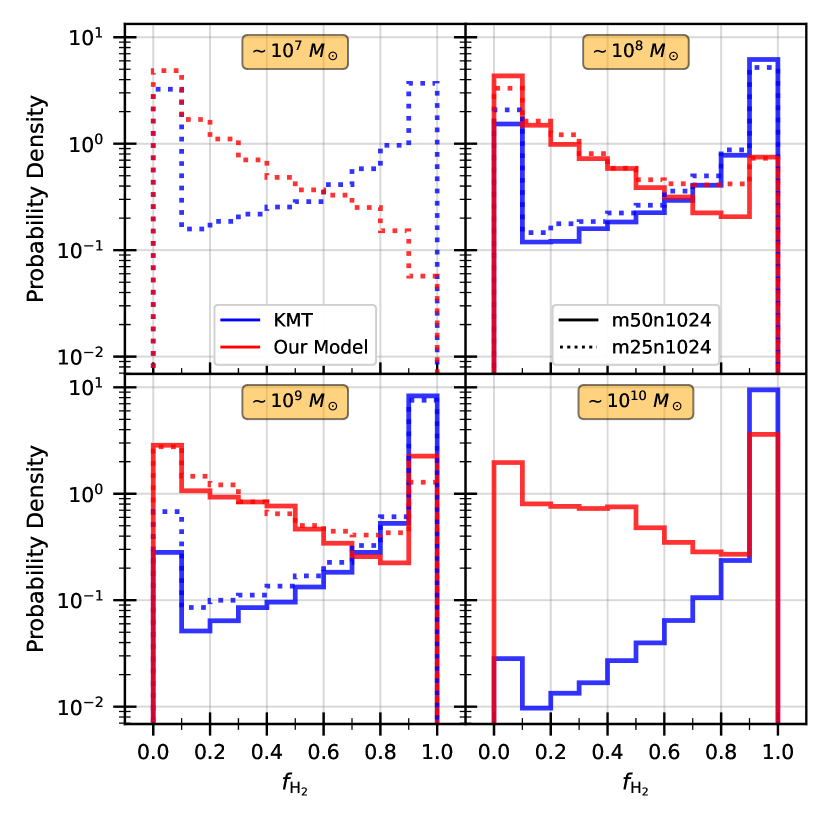
Figure 6: A histogram showing the probability density for a galactic SPH particle to contain a given fraction of H₂. The red lines show the molecular hydrogen fraction calculated using our new model, the solid and dotted lines representing data from the 50 and 25 Mpc/h boxes respectively. The blue lines show a post-processed calculation of the H₂ fraction as estimated by the KMT model for each particle in our dataset. We selected the 100 galaxies with stellar masses closest to $10^{7},10^{8},10^{9}$ and $10^{10}\,\,M_{\odot}$ to create four datasets sampling the stellar masses present in both boxes; the stellar mass of the sample is shown as an annotation on its axis. It is seen that the KMT model consistently predicts large amounts of fully molecular gas throughout the stellar mass range, whereas our model shows a procedural rise in the population of fully molecular particles with increasing stellar mass. Furthermore, the KMT model displays significantly less partially-molecular gas particles than our model, an effect which is exacerbated at large stellar masses, where we see that our model predicts a much flatter distribution.

Figure 6 shows histograms of the probability density of a galactic SPH particle possessing a H₂ fraction within one of ten equally-spaced bins. The red and blue lines show the molecular hydrogen fractions as calculated by our model during simulation run-time, and as calculated from the KMT model through post-processing, respectively. The solid lines represent results for the 50 Mpc/h box, whilst the dotted lines represent the 25 Mpc/h box. Each subplot contains the 100 closest galaxies to the stellar mass annotated on the axis, allowing us to cover a wide and representative range of galaxies in our analysis.

Focusing first on the sample of $\sim 10^{7}\,\,M_{\odot}$ galaxies, we immediately see that our model and KMT have major disagreements when $f_{\mathrm{H}_{2}}>10\%$. Whilst the KMT model predicts roughly the same amount of fully molecular as fully atomic gas (we use the terms fully molecular and fully atomic in this section to refer to the highest and lowest bins respectively, for convenience) our simulation predicts almost no fully molecular, and an abundance of fully atomic, gas. For particles with $f_{\mathrm{H}_{2}}>10\%$ we see a positive correlation with the probability density in the KMT case, and a negative correlation for our model.

As we increase the stellar mass of the galaxies in our sample, we see shifts in the behaviour mentioned for the $\sim 10^{7}\,\,M_{\odot}$ case. In the $\sim 10^{8}\,\,M_{\odot}$ sample, the KMT model is predicting significantly more particles in the fully molecular regime than the fully atomic, meaning the probability density for a particle to contain $f_{\mathrm{H}_{2}}<90\%$ falls significantly. Our models show the opposite behaviour, the population of fully molecular particles increasing dramatically, flattening the slope of the intermediate values as a result.

A continuation of these behaviours is seen in the $\sim 10^{9}\,\,M_{\odot}$ sample, the KMT model again shifting particles towards the fully molecular and away from the fully atomic. We see here that a particle pulled from the KMT model’s distribution is over $10\times$ more likely to possess $90\%<f_{\mathrm{H}_{2}}\leq 100\%$ than the next most probable bin. On the other hand, our model’s distribution is flattening, and though the population of fully molecular gas continues to increase, we do not see the exceptionally low relative probabilities exhibited in the KMT case.

Finally, the histogram containing the $\sim 10^{10}\,\,M_{\odot}$ stellar mass sample shows an extension of the effects present before. Here, the KMT model shows an exceptionally steep gradient in the probability density between its two highest bins, increasing by almost two orders of magnitude. The lower bins, including the once significant fully atomic bin are roughly $1000\times$ less likely than the fully molecular case. Conversely, the histogram for our model shows the fully molecular bin as containing only $2\times$ the probability density of its atomic counterpart. This is a significant difference between the models, KMT predicting that the vast majority of particles in massive galaxies are fully molecular. The other important distinction between the models here are their gradients. As mentioned, KMT shows a very large spike at the highest bin, and has a rapidly increasing gradient prior. Our model, however, displays a rather flat distribution, the probability density varying by roughly 0.5 dex in the range $10\%<f_{\mathrm{H}_{2}}\leq 90\%$. Whilst these intermediate bins are still less probable than the extremes, we would reasonably expect to see a large number of particles containing these fractions in our simulations; the same cannot be said for those in the KMT model.

The last observation to discuss in Figure 6 is the agreement between the simulated box sizes. Looking at the intermediate stellar mass bins (the highest and lowest contain particles from only one of the boxes due to their resolution limits) we see that in the case of both the KMT and our model, the distributions for both box sizes are in good agreement. Whilst there are discrepancies in the exact probabilities themselves, the general trends discussed above are clearly followed at both resolutions.

4.2 The H₂ Fraction’s Metallicity and Dust Scaling

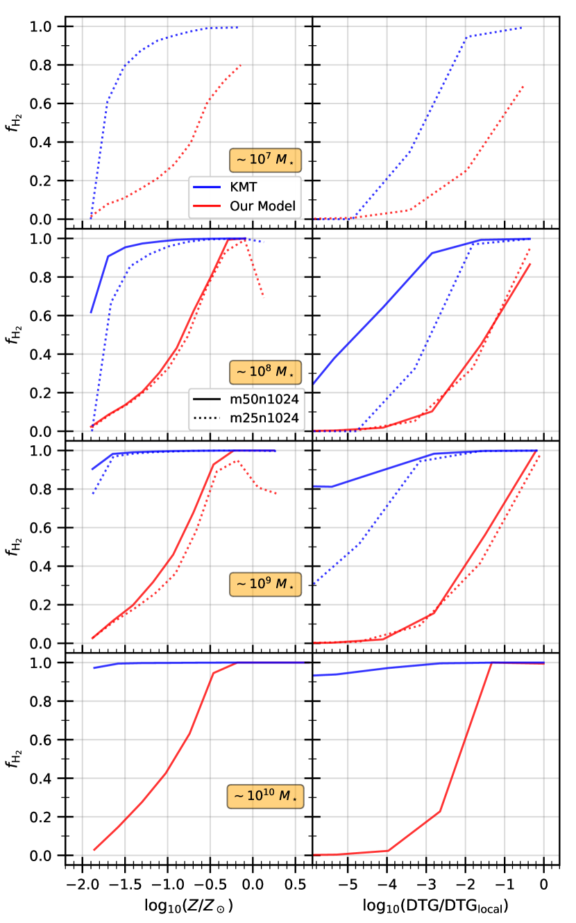
Figure 7: The dependence of metallicity and dust-to-gas ratio on the H₂ fraction in galaxies of varying stellar mass. In each row of the figure we show results for a sample of the 100 galaxies closest to the stellar mass indicated in the annotation in the left panel: these samples are identical to those presented in Figure 6. The left and right columns of the plot show how $f_{\mathrm{H}_{2}}$ varies with the metallicity and dust-to-gas ratio (normalised to the Milky Way value of Pollack et al. 1994) respectively. In each panel the x-axis is split into 10 equally-spaced bins, the median molecular hydrogen fraction within each calculated. Red and blue lines show results from our model and the KMT model respectively, with solid and dashed lines distinguishing between the simulated box-sizes as denoted on the figure.

Continuing our investigation into the modelling of molecular hydrogen, Figure 7 shows how the median H₂ fraction scales with key physical quantities across ten equally-spaced bins. In the left column we show how metallicity affects $f_{\mathrm{H}_{@}}$, and in the right column, its scaling with the dust-to-gas ratio, which we normalise to its Milky-Way value of $9.387\times 10^{-3}$ (Pollack et al., 1994). Each row of the figure represents a different sample of 100 galaxies around the stellar mass indicated by the annotation in the left panel. These samples are identical to those used in Figure 6. Blue and red lines show results from the KMT model and our model respectively, the solid and dotted lines distinguishing between the simulated box-sizes.

The top row of the figure plots the scaling relations for galaxies with stellar masses $\sim 10^{7}\,\,M_{\odot}$, on which we see an immediate disparity between the models. Whilst the molecular hydrogen content of the gas increases steadily with metallicity in our model, the KMT model shows an extremely rapid scaling, reciprocal in nature. As the metallicity increases from $Z=10^{-2}\,\,Z_{\odot}$ to $Z=10^{-3/2}\,\,Z_{\odot}$ in the KMT model, the median molecular hydrogen fraction increases from $0\%$ to $80\%$ whilst our model reaches only $10\%$ over this interval. At this stellar mass we see that the KMT model reaches the fully molecular regime at $Z\approx 10^{-1/2}$, at which point our model predicts that only $60\%$ of the hydrogen is molecular. Similar behaviour is seen when considering how the H₂ fraction scales with the dust content of the gas. The KMT model again predicts a stronger dependence on the dust-to-gas ratio when it comes to forming molecular hydrogen than our model. This is seen clearly in the gradients of the curves, and the maximal H₂ fraction reached in each case.

The $10^{8}\,\,M_{\odot}$ sample shows much the same behaviour as the $10^{7}\,\,M_{\odot}$ sample; the KMT model exhibiting an extremely rapid increase in molecular hydrogen content with metallicity, plateauing into the fully molecular regime before our model predicts a H₂ fraction of even $50\%$. A difference we do see to the previous sample however, is that our model does reach the fully molecular regime at sufficiently large metallicities. Though the gradient of the curve is much the same in both samples, the increased galactic mass has allowed for higher metal and dust content. In the KMT model, the 25 Mpc/h box scales at much the same rate in both samples also. Furthermore, we see that whilst the difference between the box-sizes in our model are generally minimal (except at the highest metallicities where resolution effects are seen), the KMT model has major disparities in both the metallicity and DTG scaling relations. For example, the 50 Mpc/h box predicts $f_{\mathrm{H}_{2}}\approx 60\%$ at $Z\approx 10^{-1.9}\,\,Z_{\odot}$, whereas the 25 Mpc/h box predicts that the hydrogen is fully atomic. A similar, though less exaggerated discrepancy can be see in the DTG scaling, where the larger box forms molecular hydrogen much more readily than its smaller counterpart.

As we move to the $10^{9}\,\,M_{\odot}$ sample we see the KMT model is now predicting much more molecular hydrogen than it was previously. Where the 25 Mpc/h box’s scaling relations didn’t change too much between the previous two samples, here we see a dramatic shift towards the fully molecular regime. In the left panel we see the KMT model predicts $f_{\mathrm{H}_{2}}>70\%$ at even the lowest metallicities, whereas our models are predicting $f_{\mathrm{H}_{2}}<5\%$. Furthermore, the right panel also shows a distinct increase in the KMT model’s gradients compared to the last sample; though this is not as pronounced as it is in the left panel. On the contrary, we see that our model, in both its metallicity and DTG scaling, displays congruent behaviour with the previous stellar mass bin, whilst showing very little resolution dependency.

The final sample shows almost no scaling with either the metallicity of dust-to-gas ratio for the KMT model, its hydrogen remaining $>90\%$ molecular in the least dusty and metallic conditions. Looking back to Figure 6, we see this behaviour manifest in the radical increase in probability between the highest two $f_{\mathrm{H}_{2}}$ bins. On the other hand, the metallicity scaling for our model is seen to remain roughly consistent with its previous behaviours at lower galactic stellar masses; whilst the gradient of the DTG scaling is seen to increase in dustier particles. Examining again the other samples, we do see that the $f_{\mathrm{H}_{2}}$ vs DTG curve for our model steepens gradually with the stellar mass of the sample. However, the same cannot be said for the metallicity relation, which remains very stable, ignoring resolution effects. Relative to the strong dependence on the stellar mass that the KMT model exhibits here, our model is largely independent of the size of the host galaxy.

5 Model Predictions: Dust and ISM Properties

In this section we investigate the dust and ISM properties calculated using our new model. To achieve this we added four new fields to the snapshot outputs written by Simba: the dust temperature, the local interstellar radiation field strength incident on the particle, and both the density and internal energy of the cool ISM component added in our two-phase model. Here we will explore the relationship between these and verify that our modelling is realistic and produces sensible, physically consistent results.

5.1 The Dust-to-Gas and Dust-to-Metal Ratios

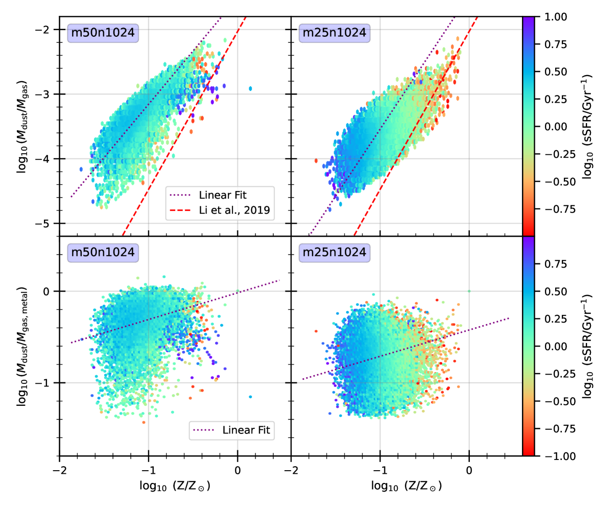
Figure 8: The dust-to-gas ratio (top row) and dust-to-metal ratio (bottom row) as a function of metallicity for galaxies identified in both our 50 (left column) and 25 (right column) Mpc/h boxes. The colour bar shows the mean specific star formation rate in each bin. The dotted purple lines are linear (in log-space) least-squares fits through the data. The red dashed line present in the top row shows the linear fit from Li et al. 2019. It is clear to see that the dust-to-gas ratio from our model grows less-steeply than that of the its predecessor. For the dust-to-metal ratios, we see that our fits highlight a relatively flat, though positively correlated dependence on metallicity.

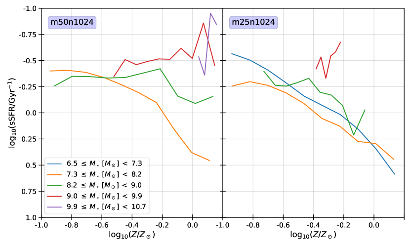
Figure 9: The median sSFR as a function of metallicity for all galaxies in each simulation box. The coloured lines ( described for each axis individually in the legend) show the dependency of galactic stellar mass on the slope of the sSFR-Z relation. It can be seen that the low-mass galaxies exhibit decreasing sSFR with increasing metallicity, whereas the largest galaxies (which are found primarily in the 50 Mpc/h box) show a positive sSFR-Z correlation. This behaviour can explain the outlying points of high metallicity and sSFR in Figure 8.

Table 2: The mathematical expression of each best fit line for the DGR as a function of metallicity – as seen in Figure 8.

Simulation	Redshift	Fit
Li et al. (2019)	0	$\log_{10}\left(\mathrm{DGR}\right)=\left(2.445\pm 0.006\right)\log_{10}\left(Z/Z_{\odot}\right)-\left(2.029\pm 0.003\right)$
This work: 50 Mpc/h box	6	$\log_{10}\left(\mathrm{DGR}\right)=\left(1.405\pm 0.005\right)\log_{10}\left(Z/Z_{\odot}\right)-\left(1.779\pm 0.006\right)$
This work: 25 Mpc/h box	6	$\log_{10}\left(\mathrm{DGR}\right)=\left(1.809\pm 0.006\right)\log_{10}\left(Z/Z_{\odot}\right)-\left(1.752\pm 0.007\right)$

In Figure 8, we find that the dust-to-gas ratio (DGR) in our model rises less steeply with metallicity than the original fit provided in Li et al. 2019; both converging toward agreement at around one solar metallicity. At low metallicity, our model produces a significantly larger DGR than the fit of Li et al., showing disparity of $\sim 1.3$ dex at $Z=0.1\,\,Z_{\odot}$ for the 50 Mpc/h box. The 25 Mpc/h box shows a result similar to, although slightly lower than, this with a $\sim 0.9$ dex disparity at identical metallicity. This discord may be largely be explained by the fact that both the original fit and our fit were computed at disparate redshifts of $z=0$ and $z=6$ respectively: Table 2 details the explicit functional form of each fit. As the metallicity approaches its solar value, $\log_{10}(Z/Z_{\odot})=0$, both fits converge to a difference of only $\sim 0.3$ dex. Furthermore, we observe that for both boxes, the (average) sSFR falls with increasing metallicity. The 50 Mpc/h box however shows a peak in the sSFR at the high-metallicity and displays a generally weaker trend than the 25 Mpc/h box in this regard.

The relationship observed in Figure 8, which shows a clear positive correlation between DGR and metallicity, is expected from physical considerations alone. We know that dust grows via accretion of metals (Section 2.5.1) and will therefore have higher abundance within gas of greater metal content. Inversely, gas with little metal will be unable to sustain high grain-accretion rates, suppressing the DGR ratio. However, there may exist physical environments in which the DGR is lower than expected for a given gaseous metal fraction. In such cases, as can be seen in Figure 8 as the points lying well below the fit, although the metal content is sufficient to sustain a larger abundance of dust, there also exists a non-negligible contribution to the destruction of grains. For example, in highly star-forming regions it may be the case that dust destruction due to thermal sputtering (which becomes more efficient in dense environments) or shocks are more/equally as potent as the rate at which the dust is being produced/grown. This scenario would result in a DGR lower than expected from the metallicity of the gas alone.

Additionally, from Figure 8 we conclude that the sSFR decreases with increasing metallicity; as can be seen most clearly in the higher-resolution 25 Mpc/h simulation. Although this result can seem somewhat perplexing upon first inspection, it is a well-observed (see Andrews & Martini 2013 for example), though non-universal relationship. In Yates et al. 2012, the slope of the metallicity-SFR relation is shown to vary with galaxy mass, becoming positive/negative in high/low-mass galaxies: which we explore further in Figure 9. Here we observe an obvious negative sSFR-Z correlation within low-mass galaxies, which turns-over at galactic stellar masses $M_{\star}\gtrsim 10^{9}M_{\odot}$ to exhibit a positive correlation; as described in the aforementioned Yates et al. 2012. Through comparison of both figures, we can deduce that the points of largest sSFR (which peak at $\sim 10\,\,\mathrm{Gyr}^{-1}$) in the 50 Mpc/h box are contributions from the most massive galaxies. It is clear then, as to why the negative sSFR-Z correlation depicted on the colour-bar of Figure 8 is more pronounced within the 25 than the 50 Mpc/h box – there is a lack of galaxies massive enough to have entered the positively-correlated regime in the smaller box.

A complex and multi-faceted analysis is required for a complete physical understanding of an individual galaxy’s placement on the DGR-Z-sSFR plane. Unfortunately, such physical discussion is beyond the scope of this paper and so we recommend reading Yates et al. 2012 for a rigorous discourse on the subject; subsequently deferring any further analysis of our own to a future work.

Complementing the above discussion on the dust-to-gas ratio, Figure 8 also presents the dust-to-metal (DTM) ratio as a function of metallicity in the bottom row of panels: the dotted line showing a least-squares fit of the data to a linear function (in log-space). The fit for both boxes display a shallow, positive correlation with a gradient of $0.292\pm 0.005$ and $0.288\pm 0.004$ for the 50 and 25 Mpc/h boxes respectively. Although the DTM ratio scales at almost the same rate in both boxes, it is clear to see that there is a large offset between them at a given metallicity. For example, the larger box estimates an equal amount of dust and gas metals, whereas the smaller box’s fit predicts $M_{\mathrm{dust}}\sim 0.4M_{\mathrm{gas,metal}}$, at solar metallicity.

The observed positive correlation between the DTM ratio and metallicity is expected from both the literature (De Vis et al., 2019; Priestley et al., 2021; Li et al., 2019) and the modelling done in our simulation. Equations 9 and 10 show that the rate of dust growth via accretion is directly proportional to the metallicity of the gas. Therefore, in high-$Z$ environments we observe considerable migration of metal from the gas to dust phase, increasing the DTM ratio.

A result of particular note is that the DTM ratio exceeds unity in the 50 Mpc/h box, showing that a small subset of galaxies in our sample possess more metallic mass in dust than they do in gas: this is not observed in the smaller box. Furthermore, we see different shapes in the distributions between box sizes, the smaller box possessing a population of high-metallicity low-DTM galaxies which are largely absent in the larger box. The existence of this population in the smaller box further validates our discourse in Section 4.2, where we argue that the abundance of dust does not necessarily increase with metallicity as its production is dependent upon stellar feedback mechanisms which are somewhat sensitive to the resolution of the simulation.

5.2 The Dust Temperature

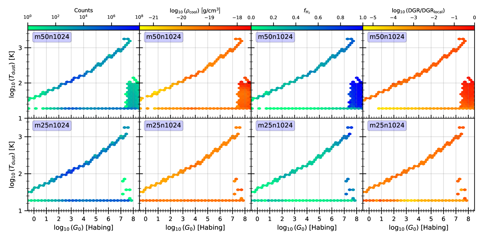
Figure 10: The dust temperature of all galactic particles as a function of the local interstellar radiation field $G_{0}$ incident upon them, for both our 50 (top row) and 25 (bottom row) Mpc/h boxes. We divide our grid into approximately regular hexagonal bins such that there are 30 along the x-axis, the colour of each quantifying the mean statistic (except for the counts). Each column of the figure places a different property on the colour bar, left-to-right these correspond to: the number of particles, the density of the cool-phase ISM gas, the molecular hydrogen fraction, and the dust-to-gas ratio scaled to that of the local universe (Pollack et al., 1994). We observe a population of high-$G_{0}$ low-$T_{\mathrm{dust}}$ particles in the larger box which are largely absent in its smaller counterpart. In both boxes, the majority of particles seem to exist along a ‘primary’ sequence for which the dust temperature is positively correlated with ISRF strength. Additionally, there exists a second sequence present at both resolutions, where the dust temperature remains constant at $\sim 10^{1.3}\approx 18$ K at all values of $G_{0}$. Comparison between columns reveals that the cool-phase density and molecular hydrogen fractions are tightly correlated as expected. Of particular note is the region of maximal molecular hydrogen abundance in the bottom-right corner of the 50 Mpc/h panel. This region does not appear in the smaller box, highlighting a significant lack of fully molecular gas as seen in Figure 7.

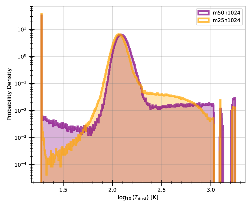
Figure 11: A histogram (500 equal-width bins) showing the dust temperature distribution of all galactic particles in both our 50 Mpc/h (purple) and 25 Mpc/h (orange) simulation boxes, as seen on the y-axis of Figure 10. The first peak at $\sim 10^{1.3}\approx 18$ K corresponds to the constant, low-temperature sequence identified in Figure 10. The abrupt, high-amplitude nature of this peak suggests that the dust is unable to cool any further than this. In both simulations we see a well defined peak at $\sim 10^{2.1}\approx 126$ K which contains significantly more probability than any other region (bar the temperature floor). Both simulations exhibit similar maximal dust temperature values of $\sim 10^{3.25}\approx 1778$ K, the 50 Mpc/h box having a slightly larger probability at this value.

We explore the relationship between the ISRF incident on gas particles in our model and the subsequent temperature of the dust they contain in Figure 10. The top and bottom rows show results from our 50 and 25 Mpc/h boxes respectively, with each column displaying a different physical quantity on the colour bar. For each panel we split the x-axis into 30 (approximately regular) hexagonal bins and calculate the mean statistic within each to display on the colour bar: except in the case of the first column which is a count of the number of particles contained within the bin. Our dataset contains all particles which are identified to exist within a galaxy.

Across all panels we identify three primary regions of interest: 1) the ‘primary’ sequence where the dust temperature is positively correlated with the ISRF strength; 2) the sequence of constant dust temperature with increasing $G_{0}$ at $\sim 10^{1.3}\approx 18$ K, the CMB temperature floor; 3) a population of high-$G_{0}$ low-$T_{\mathrm{dust}}$ particles which are not at the dust temperature floor, this region is vastly more populated in the 50 Mpc/h simulation.

Investigating first the primary sequence, we see that in both simulations, the $10^{2}\lesssim G_{0}\,\,\mathrm{Habing}\lesssim 10^{4}$ ($10^{1.8}\lesssim T_{\mathrm{dust}}\,\,\mathrm{K}\lesssim 10^{2.4}$) region contains the largest population of particles. In general, along this sequence we observe that as the ISRF strength increases, so too does the density of the cool-phase ISM and molecular hydrogen fraction. The dust-to-gas ratio does not display a noticeable dependency on $G_{0}$ in this region compared to that exhibited in others.

The sequence at which the dust temperature is constant at $\sim 10^{1.3}\mathrm{K}\left(\approx 18\mathrm{K}\right)$ for the entire range of $G_{0}$ at first seems counter-intuitive. We would expect that in general, the stronger the radiation heating the dust, the larger the dust temperature will become. However, the efficiency of the radiative cooling scales with the dust temperature and remains comparable in magnitude to the ISRF heating rate. If the dust is sufficiently sparse such that the gas-grain collisions are infrequent, heat exchange from the gas to the dust will be slow, resulting in the constant temperature behaviour we observe. It is also important to note that the temperature of this floor necessarily coincides with the CMB temperature as $T_{\mathrm{dust}}\geq T_{\mathrm{CMB}}$, which can be see in Equation 6.

Taking a look at the 50 Mpc/h run, we see that the dust-to-gas ratio increases with $G_{0}$ along this sequence, until at $G_{0}\gtrsim 10^{7}$ Habing the gas-grain coupling term becomes significant and the temperature of the dust begins to rise. We will discuss in detail the relative strengths of each heating and cooling term (see Equation 6) in Section 5.3 next.

The final region to highlight is the population of high-$G_{0}$ low-$T_{\mathrm{dust}}$ particles which exist above the temperature-floor. The size of this region varies greatly with resolution, the 50 Mpc/h run containing a much larger population here than the 25 Mpc/h run which has orders of magnitude lower particle counts. Furthermore, whereas the larger box has many populated bins (with counts $>0$) in this region, its smaller counterpart has only six. Inspecting the position of these bins carefully, we notice that the about half of these six bins do not lie within the same region as the 50 Mpc/h box; instead manifesting at marginally lower $G_{0}$.

Turning our attention to the physical properties in this region, a striking feature is the abundance of molecular hydrogen. Whilst the smaller box still reaches large abundances towards the high-$G_{0}$ end of its primary sequence, the larger exhibits a far greater population of fully-molecular gas which is absent in the former. Marrying this contrasting behaviour between resolutions back to our discussion in Section 4.2 (Figure 7 in particular) we can see that the deficiency of particles in this region leads to a lack of fully-molecular gas. As expected, this region also contains large dust-to-gas ratios which are needed to facilitate the production of molecular hydrogen.

We see a large range of interstellar radiation field strengths within our simulations, varying by $\sim 8.5$ dex from lowest to highest. In contrast, the dust temperature varies by $\sim 2$ dex at most, showing a relatively weak coupling between them. Take for example the 50 Mpc/h box’s primary sequence: at $G_{0}\approx 1$ Habing, we see that $T_{\mathrm{dust}}\sim 40$ K. If we increase the ISRF by a factor of 1000, we see that $T_{\mathrm{dust}}\sim 100$ K – an increase of only $2.5\times$. This is readily explained if we consider the case where the ISRF is dominant over all other heat sources in the heat balance equation (Equation 6); which results in $\kappa_{\mathrm{dust}}T_{\mathrm{dust}}^{4}\sim G_{0}$. For dust temperatures $<200$ K, we know that $\kappa_{\mathrm{dust}}\sim T_{\mathrm{dust}}^{2}$, therefore $T_{\mathrm{dust}}\sim G_{0}^{1/6}$. When $200<T_{\mathrm{dust}}<1500$ K we know that $\kappa_{\mathrm{dust}}\sim\mathrm{constant}$ and therefore $T_{\mathrm{dust}}\sim G_{0}^{1/4}$. We see then that the dust temperature scales more strongly with the ISRF at intermediate temperatures, however this is still a very weak power law, which explains the vast range differences between the ISRF and dust temperatures.

In addition to how the dust temperature scales with $G_{0}$, it is important that we also gain an understanding of the temperature at which the majority of the dust exists, as one of the major changes made in this work was to remove the constant dust reference temperature of 20 K previously used (see Equation 10). Figure 11 shows the probability distribution of a particle having a given dust temperature: purple and orange lines show the 50 and 25 Mpc/h simulation boxes respectively. From this we can recognise key features discussed in Figure 10 such as the high-amplitude, abrupt peak at $T_{\mathrm{dust}}\approx 10^{1.3}\sim 18K$ corresponding to the CMB temperature.

The peak at $T_{\mathrm{dust}}\approx 10^{2.1}\sim 126K$ then corresponds to the highest-count bins in the primary sequence, around which both simulations converge. However, we see that the larger box contains many more particles in the pre-peak region than the smaller box; i.e. more particles with a lower dust temperature. In contrast, the smaller box contains more particles in the post-peak domain, where the dust temperature is greater, than its larger counterpart. Looking back to Figure 10, we can see to which regions these discrepancies correspond. Most obviously, the pre-peak particles are those which sit in the high-$G_{0}$ low-$T_{\mathrm{dust}}$ population (most prevalent in the 50 Mpc/h box) and the low-tempeature end of the primary sequence. Particles absent from the high-$G_{0}$ low-$T_{\mathrm{dust}}$ population in the 25 Mpc/h box exist instead in the primary sequence, which manifests on the histogram as a peak of larger width. Post-peak we are observing the high-temperature end of the primary sequence, a region in which particles from the smaller box are more abundant until $T_{\mathrm{dust}}\approx 10^{2.7}\sim 501$ K where their population declines past that of the larger box.

Comparing the dust temperatures calculated for all particles in our simulations and the constant 20 K dust temperature used previously, we see that fiducial Simba was assuming that all particles had (approximately) the lowest dust temperature possible – our floor sitting at $\sim 18$ K. Through modelling the local ISRF for each particle and explicitly solving the gas-grain heat balance to calculate the dust temperature, we find dust temperatures two orders of magnitude larger than was previously assumed. Furthermore, we see that particles existing above the temperature floor are likely to posses a dust temperature of $\sim 126$ K, roughly six times the assumed reference value. Order-of-magnitude changes in the dust temperature will subsequently increase the characteristic timescale at which dust grains accrete gas-phase metals (Equation 10), ultimately decreasing the growth rate. Observations of high-redshift, dusty galaxies have shown the existence of a large population of hot dust (Viero et al., 2022; Jones et al., 2023) in the early universe. The modelled polynomial relationship between the dust temperature and redshift reported in Viero et al. 2022 results in an estimate of $T_{\mathrm{dust}}\sim 74$ K at redshift 6, whilst the redshift $\sim 8.31$ observations from Jones et al. 2023 measure dust temperatures $\gtrsim 90$ K. Whilst not as hot as the temperatures we are commonly seeing in our simulations, these observations are a clear departure from the $\sim 20$ K values thought to be representative; further demonstrating the need for sophisticated dust treatment. Moreover, the sample of observed galaxies are likely not representative of our simulated sample as we are not bound by observational constraints. To offer a like-for-like comparison we would need to think carefully about our target selection in order to mimic that carried out in these works.

5.3 Dissecting the Gas-Grain Heat Balance

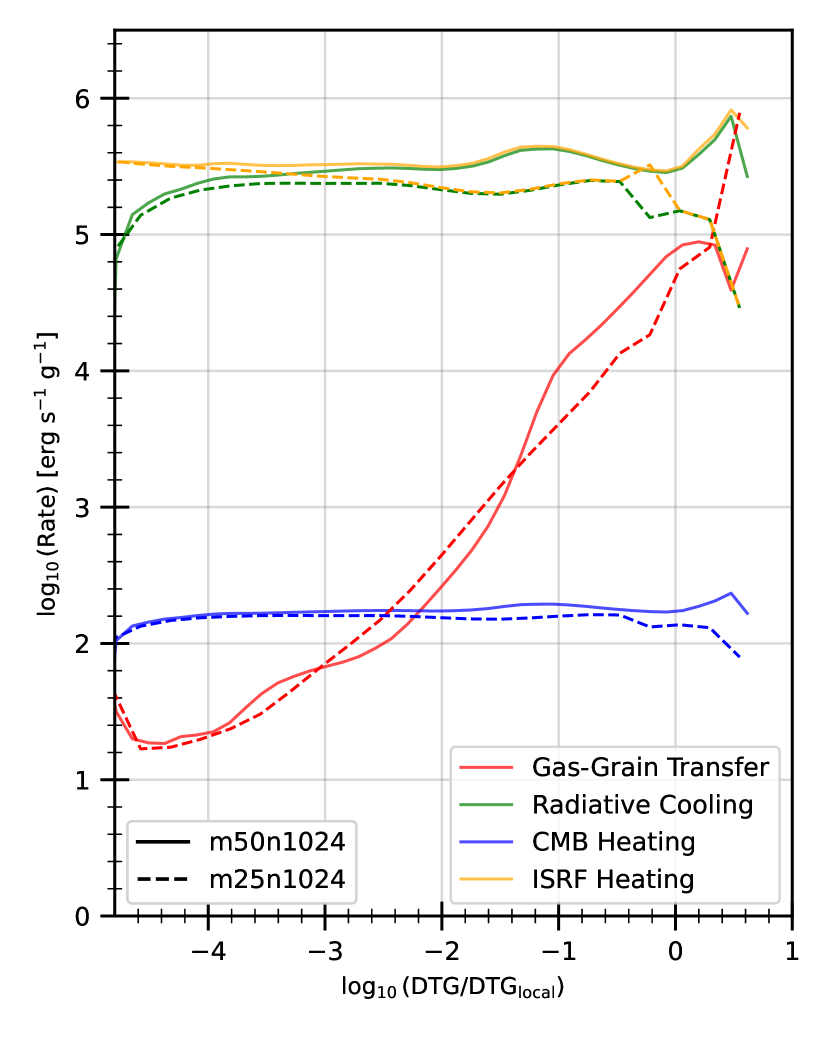
Figure 12: The median dust heating and cooling rate for all galactic particles in both our 50 Mpc/h and 25 Mpc/h runs, displayed by the solid and dashed lines respectively, as a function of the dust-to-gas ratio normalised to the value observed in the local universe (Pollack et al., 1994). To compute the median rate we sort the data by its dust-to-gas ratio into 100 regular bins. Each term present in the heat balance equation (see Equation 6) are displayed as follows: the gas-grain heat transfer in red; the radiative cooling in green; the radiative heating from the CMB in blue, and the radiative heating from the ISRF in orange.

The radiative cooling term shown in Figure 12, which describes the heat emitted from the grains, is in steady-state thermal equilibrium with the heating terms by construction. In fact, this is how the dust temperature is calculated in Equation 6, and therefore we know that the cooling rate should trace the net heating rate. As the heating is dominated by the ISRF in our case, it should come as no surprise that the cooling rate follows the ISRF heating rate closely. We do see, however, marginal fluctuations between the cooling and ISRF heating terms. It is reasonable to believe that these emerge as a result of minor variations in the physical conditions present. Furthermore, due to the necessity of heat balance, we know that the ISRF (in our case) is responsible for setting the dust temperature. This means that the high dust temperature values present in our simulation could possibly arise from an overestimation of $G_{0}$.

As mentioned above, we see that the ISRF is the dominant source of heating across the range of dust abundances present, its heating rate remaining constant at $\sim 10^{5.6}$ and $\sim 10^{5.4}\,\,\mathrm{erg}\,\mathrm{s}^{-1}\,\mathrm{g}^{-1}$ for the 50 and 25 Mpc/h boxes respectively when $\log_{10}(\mathrm{DTG}/\mathrm{DTG}_{\mathrm{local}})<0$. At high densities, $\log_{10}(\mathrm{DTG}/\mathrm{DTG}_{\mathrm{local}})\gtrsim 0$, we see divergent behaviour between our simulations. The smaller box’s heating rate falls to $\sim 10^{4.5}\,\,\mathrm{erg}\,\mathrm{s}^{-1}\,\mathrm{g}^{-1}$ by $\log_{10}(\mathrm{DTG}/\mathrm{DTG}_{\mathrm{local}})\approx 10^{0.6}$, whilst the larger box’s increases to $\sim 10^{5.9}\,\,\mathrm{erg}\,\mathrm{s}^{-1}\,\mathrm{g}^{-1}$. Referring back to Figure 10, we see that the 50 Mpc/h box contains a larger number of particles with a dust-to-gas ratio exceeding that of the local ISM value than its 25 Mpc/h counterpart. Furthermore, the smaller box’s most dust abundant particles occur at low-ISRF values; a contrast to their occurrence at high-ISRF values in the larger box. These characteristics explain the discrepant behaviour seen between the boxes at the largest dust abundances. To understand why the ISRF heating rate is generally lower in the 25 Mpc/h box (at all dust abundances) we refer back to Figure 1, where it is shown that the larger box contains more particles with intermediate-high SFRs and stellar masses than the smaller. Given that we calculate the ISRF incident on a particle by the sSFR of its neighbouring particles (Equation 8) it follows that, generally, galactic particles in the 50 Mpc/h box will be irradiated by larger ISRFs than those in the 25 Mpc/h box.

The rate at which the CMB heats the dust is negligible relative to that of the ISRF. Remaining constant at $\sim 10^{2.2}\,\,\mathrm{erg}\,\mathrm{s}^{-1}\,\mathrm{g}^{-1}$ while $\log_{10}(\mathrm{DTG}/\mathrm{DTG}_{\mathrm{local}})\lesssim-2$, there is no appreciable difference between the simulation boxes. However, as $\log_{10}(\mathrm{DTG}/\mathrm{DTG}_{\mathrm{local}})>-2$ the 25 Mpc/h box is seen to remain constant whilst the 50 Mpc/h box’s heating rate increases marginally. Similar to the behaviour displayed for the ISRF, the smaller box’s CMB heating rate drops appreciably at for the most dust-abundant particles whilst the larger box’s spikes in this regime. The CMB temperature is constant across all particles – given that it is inversely proportional to the cosmological scale factor $T_{\mathrm{CMB}}=T_{0}\left(1+Z\right)$ – and so any inter-particle variance in its heating rate arises from differences in the grain opacity (see Equation 5). Given that its heating rate is $\sim 3$ dex lower than that of the ISRF, it has a negligible contribution to the overall heat balance. However, this does highlight the relevance of the ISRF’s inclusion; without which we would find vastly different dust temperatures to those presented in this work.

The final heating term describes the rate of energy transfer as the gas and grains collide. Unlike the previous terms discussed, this can act to either heat or cool the gas depending on the direction of the temperature gradient. Furthermore, due to the collisional nature of this process, we expect a strong positive correlation with the dust-to-gas ratio, which is clearly seen in Figure 12. For example, within dust-sparse gas, $\log_{10}(\mathrm{DTG}/\mathrm{DTG}_{\mathrm{local}})<-3$, the collisional heating rate is entirely negligible relative to the other terms, contributing even less than the CMB radiation. However, in dust-rich environments $\log_{10}(\mathrm{DTG}/\mathrm{DTG}_{\mathrm{local}})>0$ the gas-grain heat exchange is significant, reaching rates comparable to that of the ISRF radiation’s heating. Slight variations between the two simulated resolutions are observed across the range of dust abundances. The high-resolution run shows a consistent linear scaling, whilst the low-resolution run’s median appears more turbulent. Given that collisional processes such as these are highly dependent on environmental specifics, fluctuations in the collisional heating rate between regions of identical dust-to-gas ratio are expected.

6 Conclusions

We have implemented a novel procedure to model the chemical and thermodynamic evolution of the interstellar medium within the Simba simulations (Davé et al., 2019). Specifically, our model aims to treat dust and molecular hydrogen in a self-consistent manner. This is achieved through integration of Grackle’s (Smith et al., 2017) molecular hydrogen network, which follows the most important formation channels for H₂, including its formation on the surface of dust grains. The molecular hydrogen fraction is used to drive the formation of stars, which themselves emit radiation into the interstellar medium, heating the dust. The dust population grows through the accretion of gas-phase metals, the rate of which is determined, in part, by the temperature of the dust itself. As the dust population grows, the chance of a hydrogen-grain collision increases, thereby accelerating the rate at which H₂ forms.

We ran two simulations from $z=99$ to $z=6$, both containing 1024³ baryonic and dark matter particles but differing in the size of their simulated boxes: one possessing a side-length of 25 Mpc/h and the other 50 Mpc/h. We confirm that our simulations are consistent with key Simba results (see Section 3) in addition to observation through comparison of the SFR, dust and stellar mass functions. We find that our model reproduces the galactic mass functions seen in fiducial Simba to good accuracy, and follows observed data with reasonable consistency. By running photometry on the galaxies identified in our simulations and analysing their UV luminosity functions, we find that the brightest observed sources which have proved difficult to reproduce previously are reasonably well modelled in our work at redshift 6. Furthermore, we see close agreement between the simulated UV luminosity functions and observed datapoints at redshift 11 and 6, with a clear evolution between the two at intermediate redshifts.

We post-process our runs using yt to compute the KMT-estimated H₂ fraction for each gas particle within a sample of identified galaxies (see Section 4). We find that, compared with the results obtained by solving the chemical network, the KMT model underestimates the number of particles with $0.8<f_{\mathrm{H}_{2}}\leq 1.0$ and overestimates those with $0.0<f_{\mathrm{H}_{2}}\leq 0.2$. The underestimation of the molecular hydrogen content within a particle will result in a corresponding underestimation of the star formation rate due Simba’s H₂ driven SFR model. We show the differences between the molecular hydrogen fraction’s scaling with both the metallicity and dust-to-gas ratio in both models. The KMT model exhibits a steeper gradient than Grackle in all cases, transitioning from the atomic to molecular regime at considerably larger metallicity/DGR also. Furthermore, where Grackle shows only slight resolution dependence in its scaling, the KMT model’s results vary massively between resolution, highlighting the robust nature of an explicit, physically motivated approach.

Finally, we investigate the ISM gas and dust properties within our new model (see Section 5). We find that the interstellar radiation field strength incident on galactic particles vary greatly from $10^{1}-10^{8}$ Habing, with most being subject to strengths of $10^{3}$ Habing. At the largest ISRF strengths we notice a striking resolution-dependent population with temperatures $\sim 20$ K that is present in the larger box but almost entirely absent in the smaller. This population contains the majority of large DGR and $f_{\mathrm{H}_{2}}$ gas, and as such the 25 Mpc/h box does not show dust and H₂ abundances as large as its 50 Mpc/h counterpart. We show that the average dust temperature in both simulations is $\sim 126$ K, an order-of-magnitude larger than the 20 K reference temperature used in the fiducial Simba dust model. A discrepancy this large will affect the dust accretion rate considerably; in turn modifying the fraction of metal in the gas and dust phases. Moreover, the dust temperature is shown to vary from $\sim 20-1580$ K, highlighting the vast environmental differences which are being neglected when employing constant reference values. Lastly, we dissect the gas-grain heat balance which is solved to give the dust temperature. We find that the ISRF’s contribution is dominant over all other heating terms except in the most dust-rich environments where gas-grain collisions are frequent enough to facilitate inter-phase heat exchange.

There are many avenues to be explored in continuing this work into the future, the most immediate being the low-redshift behaviour of our model. Secondly, confirmation/enhancement of the ISRF model is a crucial task in the continuation of this work. Whilst the calculation implemented is well motivated and does not yield unphysical results, the overwhelming significance of the ISRF’s contribution to dust heating necessitates further work. The addition of an explicit luminosity-driven calculation (as discussed in 2.4) is an obvious candidate for such work. Furthermore, the ISRF goes hand-in-hand with the issue of dust shielding, the KMT approximation for which (a scaling with surface metal density) was removed in this work. Essentially, the effect of dust shielding is to attenuate the ISRF heating term in the heat balance equation (Equation 6). Implementing a justified and self-consistent calculation of this attenuation will be important in future works. Finally, the last suggestion we will offer here is a rigorous investigation into the cause of the resolution-dependencies highlighted in this work – that of the disparate high-$G_{0}$ low-$T_{\mathrm{dust}}$ population shown in Figure 10 being of particular note. As this population contains the vast majority of fully-molecular and dust-abundant gas particles, it is important that we understand the physical conditions which lead to its existence (or lack thereof); an investigation which was beyond the scope of this work.

Software

To analyse our results we used the following astrophysical Python packages: yt (Turk et al., 2011a) for handling of the raw data contained within simulation snapshots; Caesar to identify and group particles into galaxies and halos for analysis; pyloser , an extension of CAESAR which uses fsps (Conroy et al., 2009; Conroy & Gunn, 2010) to compute photometry on identified galaxies; and Matplotlib (Hunter, 2007) to create the figures.

Data Availability

The simulation snapshots, galaxy catalogues and codes from which this work was composed is stored locally, but can be made available to any interested parties upon reasonable request to the authors.

Appendix A The Dust Accretion Timescale and Sticking Potential

Consider the following situation, spherical dust grains of constant mass density grow through the accretion of gas-phase metals on their surface. The collisional cross-sections of these grains are equal to their geometrical cross-sections, ie. we do not consider electrostatic forces. The composition of the grain determines which metal it must accrete in order to grow, this metal is known as the ‘key species‘, denoted by $\mathrm{X}$ in our equations (Zhukovska et al., 2008). When a gas-phase metal strikes a grain, there is a probability, $\xi(T_{\mathrm{gr}},T_{\mathrm{X}})$, that it remains bound to the surface, we call this the ‘sticking potential’.

With these assumptions in mind, we can construct the rate at which gas-phase metals strike the grain surface as,

$$R_{\mathrm{coll}}=\pi a^{2}\braket{v_{\mathrm{X}}}n_{\mathrm{X}}$$ (16)

where $a$ is the radius of the grain, $\braket{v_{\mathrm{X}}}$ is the average speed of the key gas-phase metals, and $n_{\mathrm{X}}$ is their corresponding number density (Hirashita & Kuo, 2011; Asano et al., 2013). We can then write the rate at which the gaseous metal population is depleted through accretion as,

$$\frac{dm_{\mathrm{acc}}}{dt}=R_{\mathrm{coll}}m_{\mathrm{X}}\xi(T_{\mathrm{gr}},T_{\mathrm{X}})$$ (17)

where $m_{\mathrm{X}}$ is the atomic mass of the key metal species. As we do not model different grain compositions in our simulation, we simply assume that the accreted species are split equally among the metals present. This allows us to write $n_{\mathrm{X}}m_{\mathrm{X}}=\rho_{\mathrm{g}}Z_{\mathrm{g}}$ where $\rho_{\mathrm{g}}$ is the mass density of the gas and $Z_{\mathrm{g}}$ is the gas metallicity. Furthermore, we assume that the metals are in thermal equilibrium with the gas. Combining equations 16 and 17 with these assumptions we obtain,

$$\frac{dm_{\mathrm{acc}}}{dt}\sim\pi a^{2}T_{\mathrm{g}}^{1/2}\rho_{\mathrm{g}}Z_{\mathrm{g}}\xi(T_{\mathrm{gr}},T_{\mathrm{g}})$$ (18)

where we set $\braket{v_{\mathrm{g}}}\sim T_{\mathrm{g}}^{1/2}$ assuming the gas follows a Maxwell-Boltzmann distribution.

We now turn our attention to the rate at which the grains themselves grow through accretion. The mass of a spherical grain with constant mass density, $\sigma$, is simply given by $m_{\textrm{gr}}=4/3\pi a^{3}\sigma$. Differentiating this with respect to time we find,

$$\frac{dm_{\mathrm{gr}}}{dt}=4\pi a^{2}\dot{a}\sigma$$ (19)

where $\dot{a}\equiv da/dt$. Assuming the grains only grow through accretion, we know that the rate at which metals are depleted from the gas due to accretion must equal the growth rate of the grain. This means that we can equate equations 18 and 19, then rearrange to find,

$$\dot{a}\sim\frac{1}{4\sigma}\rho_{\mathrm{g}}Z_{\mathrm{g}}T_{\mathrm{g}}^{1/2}\xi(T_{\mathrm{gr}},T_{\mathrm{g}}).$$ (20)

The dust accretion timescale is defined as $\tau_{\mathrm{acc}}\equiv a/\dot{a}$. Using the above equation we obtain,

$$\tau_{\mathrm{acc}}\simeq\tau_{\mathrm{acc,0}}\xi^{-1}(T_{\mathrm{gr}},T_{\mathrm{g}})\left(\frac{\rho_{\mathrm{ref}}}{\rho_{\mathrm{g}}}\right)\left(\frac{Z_{\mathrm{ref}}}{Z_{\mathrm{g}}}\right)\left(\frac{T_{\mathrm{ref}}}{T_{\mathrm{g}}}\right)^{1/2}$$ (21)

where we have inserted three characteristic reference values to determine the specific normalisation of the density, metallicity and temperature individually. Furthermore, we have added an overall normalisation to the accretion rate, $\tau_{\mathrm{acc,0}}$. The three reference values should be chosen such that they represent typical values in the physical scenarios being modelled. The accretion rate normalisation should be set to a reasonable value and tuned to suit the specific use case.

We do this parameterisation to leave us with an equation akin to that prevalent in the literature (Li et al., 2019; Asano et al., 2013). Note that as we do not model a grain size distribution, the radius of the grain is absorbed into this normalisation. However, we have not assumed that the sticking potential is unity, as is typically done in the literature. This is because it depends on the grain temperature, a parameter of key focus in our work.

As discussed in Section 2.5.1, the exact form of the sticking potential is incredibly complex, so much so that it is impracticable to include in our current simulations which do not track grain compositions or the grain size distribution, in addition to the chemistry or cooling required for grains of specific compositions. We can reason however, that in general, the sticking potential must depend on the energy of the metal-grain collision. If they collide violently, at high energies, then we expect there to be a low probability that the metal will remain bound to the grain surface. Oppositely, if the collision takes place at low energies, the metal will have a high chance of remaining bound to the grain.

The hydrogen-grain sticking potential presented in Hollenbach & McKee 1979 is a good example of such behaviour,

$$\xi(T_{\mathrm{gr}},T_{\mathrm{g}})\sim\frac{1}{\sqrt{T_{\mathrm{gr}}+T_{\mathrm{g}}}+1}$$ (22)

where we have neglected to include the higher-power terms of $T_{\mathrm{g}}$ presented in the original paper for simplicity. We see that this equation behaves as reasoned above – as the total temperature approaches zero, the sticking potential approaches unity, ie. there is a 100% chance that the metal remains bound to the grain surface. Oppositely, as the temperature of one or both of the particles approaches infinity, the sticking potential approaches zero, ie. the metal will never remain bound to the grain surface.

However, the issue with implementing this equation into our model is its dependence on the gas temperature, which would affect the accretion timescale’s behaviour significantly. A complete inclusion of the sticking potential, as a function of both the gas and grain temperatures, would require the development and implementation of an entirely different model designed for this purpose. We therefore make the choice to adopt a sticking potential of the form,

$$\xi(T_{\mathrm{gr}})\sim T_{\mathrm{gr}}^{-1/2}\,.$$ (23)

which introduces only a weak scaling with the dust temperature, ensuring the continued validity of the model with these changes. We can then re-write the accretion timescale as,

$$\tau_{\mathrm{acc}}\simeq\tau_{\mathrm{ref}}\left(\frac{\rho_{\mathrm{ref}}}{\rho_{\mathrm{g}}}\right)\left(\frac{Z_{\mathrm{ref}}}{Z_{\mathrm{g}}}\right)\left(\frac{T_{\mathrm{gr}}}{T_{\mathrm{g}}}\right)^{1/2}$$ (24)

where $\tau_{\mathrm{acc,0}}$ has been re-tuned to give $\tau_{\mathrm{ref}}$. Comparing this with equation 21 you will see that in total we have essentially set $T_{\mathrm{ref}}=T_{\mathrm{gr}}$; this is the claim we make in Section 2.5.1.

In conclusion, whilst we want the dust temperature to appear in the accretion rate equation (as it makes intuitive sense for this to be the case and provides better self-consistency between models) we carry this out in the simplest way possible. We have made many simplifying assumptions in lieu of fully modelling the grain sizes and compositions, and taken advantage of the fact that the model of Li et al. 2019 is sub-grid with four free-parameters which require tuning. A result of this inherent ambiguity is that we can add a simple dependence on the dust temperature, which acts to increase/decrease the rate of accretion subtly, whilst allowing the rest of our dust model to feed back to the rate at which it grows. To ensure the validity of our model after these changes, we re-tuned the $\tau_{\mathrm{acc,0}}$ parameter (renaming it $\tau_{\mathrm{ref}}$ for clarity) such that the redshift $\sim 6$ stellar mass function it predicts is in alignment with contemporary results from both observation and simulation.

References

- Agertz et al. (2007) Agertz O., et al., 2007, Monthly Notices of the Royal Astronomical Society, 380, 963
- Andrews & Martini (2013) Andrews B. H., Martini P., 2013, The Astrophysical Journal, 765, 140
- Asano et al. (2013) Asano R. S., Takeuchi T. T., Hirashita H., Inoue A. K., 2013, Earth, Planets and Space, 65, 213
- Bate & Burkert (1997) Bate M. R., Burkert A., 1997, MNRAS, 288, 1060
- Bouwens et al. (2015) Bouwens R. J., et al., 2015, The Astrophysical Journal, 803, 34
- Bromm (2013) Bromm V., 2013, Reports on Progress in Physics, 76, 112901
- Collaboration et al. (2014) Collaboration T. E., et al., 2014, The Astrophysical Journal Supplement Series, 211, 19
- Conroy & Gunn (2010) Conroy C., Gunn J. E., 2010, ApJ, 712, 833
- Conroy et al. (2009) Conroy C., Gunn J. E., White M., 2009, ApJ, 699, 486
- Davé et al. (2016) Davé R., Thompson R. J., Hopkins P. F., 2016, Monthly Notices of the Royal Astronomical Society, 462, 3265
- Davé et al. (2019) Davé R., Anglés-Alcázar D., Narayanan D., Li Q., Rafieferantsoa M. H., Appleby S., 2019, Monthly Notices of the Royal Astronomical Society, 486, 2827
- De Vis et al. (2019) De Vis P., et al., 2019, Astronomy & Astrophysics, 623, A5
- Dekel et al. (2023) Dekel A., Sarkar K. C., Birnboim Y., Mandelker N., Li Z., 2023, Monthly Notices of the Royal Astronomical Society, 523, 3201
- Donnan et al. (2022) Donnan C. T., et al., 2022, Monthly Notices of the Royal Astronomical Society, 518, 6011
- Dopcke et al. (2011) Dopcke G., Glover S. C. O., Clark P. C., Klessen R. S., 2011, The Astrophysical Journal, 729, L3
- Draine & Salpeter (1979) Draine B. T., Salpeter E. E., 1979, The Astrophysical Journal, 231, 77
- Dwek (1998) Dwek E., 1998, The Astrophysical Journal, 501, 643
- Ferland et al. (2013) Ferland G. J., et al., 2013, The 2013 Release of Cloudy, http://arxiv.org/abs/1302.4485
- Ferrara et al. (2023) Ferrara A., Pallottini A., Dayal P., 2023, Monthly Notices of the Royal Astronomical Society, 522, 3986
- Finkelstein et al. (2023) Finkelstein S. L., et al., 2023, The Complete CEERS Early Universe Galaxy Sample: A Surprisingly Slow Evolution of the Space Density of Bright Galaxies at z ~ 8.5-14.5, http://arxiv.org/abs/2311.04279
- Galli & Palla (1998) Galli D., Palla F., 1998, The Chemistry of the Early Universe, http://arxiv.org/abs/astro-ph/9803315
- Gardner et al. (2006) Gardner J. P., et al., 2006, Space Science Reviews, 123, 485
- Habing (1968) Habing H. J., 1968, Bull. Astron. Inst. Netherlands, 19, 421
- Harikane et al. (2022) Harikane Y., et al., 2022, The Astrophysical Journal Supplement Series, 259, 20
- Hirashita (2000) Hirashita H., 2000, Publications of the Astronomical Society of Japan, 52, 585
- Hirashita & Kuo (2011) Hirashita H., Kuo T.-M., 2011, Monthly Notices of the Royal Astronomical Society, 416, 1340
- Hollenbach & McKee (1979) Hollenbach D., McKee C. F., 1979, The Astrophysical Journal Supplement Series, 41, 555
- Hollenbach & McKee (1989) Hollenbach D., McKee C. F., 1989, The Astrophysical Journal, 342, 306
- Hopkins & Raives (2016) Hopkins P. F., Raives M. J., 2016, Monthly Notices of the Royal Astronomical Society, 455, 51
- Hu et al. (2019) Hu C.-Y., Zhukovska S., Somerville R. S., Naab T., 2019, Monthly Notices of the Royal Astronomical Society, 487, 3252
- Hunter (2007) Hunter J. D., 2007, Computing in Science & Engineering, 9, 90
- Jones & Nuth (2011) Jones A. P., Nuth J. A., 2011, Astronomy & Astrophysics, 530, A44
- Jones et al. (2023) Jones G. C., Witstok J., Concas A., Laporte N., 2023, New constraints on the molecular gas content of a $z\sim8$ galaxy from JVLA CO(J=2-1) observations, http://arxiv.org/abs/2312.05012
- Kannan et al. (2022) Kannan R., Garaldi E., Smith A., Pakmor R., Springel V., Vogelsberger M., Hernquist L., 2022, Monthly Notices of the Royal Astronomical Society, 511, 4005
- Krumholz (2014) Krumholz M. R., 2014, Monthly Notices of the Royal Astronomical Society, 437, 1662
- Krumholz & Gnedin (2011) Krumholz M. R., Gnedin N. Y., 2011, The Astrophysical Journal, 729, 36
- Krumholz et al. (2009) Krumholz M. R., McKee C. F., Tumlinson J., 2009, The Astrophysical Journal, 693, 216
- Langeroodi et al. (2022) Langeroodi D., et al., 2022, Evolution of the Mass-Metallicity Relation from Redshift $z\approx8$ to the Local Universe, http://arxiv.org/abs/2212.02491
- Leitherer et al. (1999) Leitherer C., et al., 1999, The Astrophysical Journal Supplement Series, 123, 3
- Li et al. (2019) Li Q., Narayanan D., Davé R., 2019, Monthly Notices of the Royal Astronomical Society, 490, 1425
- Licquia & Newman (2015) Licquia T. C., Newman J. A., 2015, The Astrophysical Journal, 806, 96
- Madau & Dickinson (2014) Madau P., Dickinson M., 2014, Annual Review of Astronomy and Astrophysics, 52, 415
- McKee (1989) McKee C. F., 1989, Symposium - International Astronomical Union, 135, 431
- McLeod et al. (2023) McLeod D. J., et al., 2023, The galaxy UV luminosity function at $\mathbf{z \simeq 11}$ from a suite of public JWST ERS, ERO and Cycle-1 programs, http://arxiv.org/abs/2304.14469
- Navarro-Carrera et al. (2023) Navarro-Carrera R., Rinaldi P., Caputi K. I., Iani E., Kokorev V., van Mierlo S. E., 2023, Constraints on the Faint End of the Galaxy Stellar Mass Function at z ~ 4-8 from Deep JWST Data, http://arxiv.org/abs/2305.16141
- Olsen et al. (2017) Olsen K. P., Greve T. R., Narayanan D., Thompson R., Davé R., Rios L. N., Stawinski S., 2017, The Astrophysical Journal, 846, 105
- Pillepich et al. (2018) Pillepich A., et al., 2018, Monthly Notices of the Royal Astronomical Society, 473, 4077
- Pollack et al. (1994) Pollack J. B., Hollenbach D., Beckwith S., Simonelli D. P., Roush T., Fong W., 1994, ApJ, 421, 615
- Priestley et al. (2021) Priestley F. D., De Looze I., Barlow M. J., 2021, Monthly Notices of the Royal Astronomical Society: Letters, 509, L6
- Romano et al. (2022) Romano L. E. C., Nagamine K., Hirashita H., 2022, Monthly Notices of the Royal Astronomical Society, 514, 1461
- Schaye et al. (2015) Schaye J., et al., 2015, Monthly Notices of the Royal Astronomical Society, 446, 521
- Schneider et al. (2006) Schneider R., Omukai K., Inoue A. K., Ferrara A., 2006, Monthly Notices of the Royal Astronomical Society, 369, 1437
- Slavin et al. (2015) Slavin J. D., Dwek E., Jones A. P., 2015, The Astrophysical Journal, 803, 7
- Smith et al. (2017) Smith B. D., et al., 2017, Monthly Notices of the Royal Astronomical Society, 466, 2217
- Spitzer (2004) Spitzer L., 2004, Physical processes in the interstellar medium. Physics textbook, Wiley, Weinheim
- Springel & Hernquist (2003) Springel V., Hernquist L., 2003, Monthly Notices of the Royal Astronomical Society, 339, 289
- Springel et al. (2021) Springel V., Pakmor R., Zier O., Reinecke M., 2021, Monthly Notices of the Royal Astronomical Society, 506, 2871
- Stefanon et al. (2021) Stefanon M., Bouwens R. J., Labbé I., Illingworth G. D., Gonzalez V., Oesch P. A., 2021, The Astrophysical Journal, 922, 29
- Tegmark et al. (1997) Tegmark M., Silk J., Rees M., Blanchard A., Abel T., Palla F., 1997, The Astrophysical Journal, 474, 1
- Tielens & Hollenbach (1985) Tielens A. G. G. M., Hollenbach D., 1985, The Astrophysical Journal, 291, 722
- Tielens et al. (1994) Tielens A. G. G. M., McKee C. F., Seab C. G., Hollenbach D. J., 1994, The Astrophysical Journal, 431, 321
- Tsai & Mathews (1995) Tsai J. C., Mathews W. G., 1995, The Astrophysical Journal, 448, 84
- Turk et al. (2011a) Turk M. J., Smith B. D., Oishi J. S., Skory S., Skillman S. W., Abel T., Norman M. L., 2011a, The Astrophysical Journal Supplement Series, 192, 9
- Turk et al. (2011b) Turk M. J., Clark P., Glover S. C. O., Greif T. H., Abel T., Klessen R., Bromm V., 2011b, The Astrophysical Journal, 726, 55
- Viero et al. (2022) Viero M. P., Sun G., Chung D. T., Moncelsi L., Condon S. S., 2022, Monthly Notices of the Royal Astronomical Society: Letters, 516, L30
- Yates et al. (2012) Yates R. M., Kauffmann G., Guo Q., 2012, Monthly Notices of the Royal Astronomical Society, 422, 215
- Zhukovska et al. (2008) Zhukovska S., Gail H.-P., Trieloff M., 2008, Astronomy & Astrophysics, 479, 453