Optimising quantum tomography via shadow inversion

Abstract

In quantum information theory, the accurate estimation of observables is pivotal for quantum information processing, playing a crucial role in compute and communication protocols. This work introduces a novel technique for estimating such objects, leveraging an underutilised resource in the inversion map of classical shadows that greatly refines the estimation cost of target observables without incurring any additional overhead. A generalised framework for computing and optimising additional degrees of freedom in the homogeneous space of the shadow inversion is given that may be adapted to a variety of near-term problems. In the special case of local measurement strategies we show feasible optimisation leading to an exponential separation in sample complexity versus the standard approach and in an exceptional case we give non-trivial examples of optimised post-processing for local measurements, achieving the same efficiency as the global Cliffords shadows.

Introduction

Quantum state tomography with classical shadows Huang et al. (2020), initially motivated by the seminal work of Aaronson Aaronson (2017), represents a significant advancement in the realm of quantum information processing, particularly in the efficient characterisation of quantum systems. This technique, developed as a solution to the prohibitive resource requirements of full quantum state tomography has since seen a plethora of modifications Hu et al. (2023); Elben et al. (2020); Huang et al. (2021); Neven et al. (2021); Crawford et al. (2021); Chen et al. (2021); Hadfield et al. (2022); Zhao et al. (2021); Seif et al. (2023); Wan et al. (2023); Levy et al. (2024); Bu et al. (2024); Coopmans et al. (2023); Bertoni et al. (2023); Koh and Grewal (2022); McGinley and Fava (2023); Kunjummen et al. (2023); Iosue et al. (2024); Nakaji et al. (2023); Feldman et al. (2022); Wyderka et al. (2023), which all seek to provide a viable alternative for obtaining meaningful information about quantum states with substantially reduced computational and experimental overhead Sack et al. (2022); Anshu et al. (2021); Huang et al. (2023); Nguyen et al. (2022); Zhang et al. (2021); Struchalin et al. (2021); Stilck França et al. (2024); Ippoliti et al. (2023); Morris et al. (2022); Glos et al. (2022); Stricker et al. (2022); Vermersch et al. (2023). Naturally, the main focus has been the ’quantum’ element of the procedure as this is where most practical efforts are stymied, either in gate or sample complexity. Other than machine learning Huang et al. (2023, 2022) and adaptive techniques García-Pérez et al. (2021); Glos et al. (2022), little thought has been put towards explicit optimisation of the classical postprocessing with it often being treated as a mostly fixed step.

At the core of shadow tomography lies the concept of constructing these aforementioned shadows; efficiently representable compressed classical descriptions of quantum states. These shadows are generated through a process involving random measurements on copies of a state, followed by classical processing to reconstruct a succinct representation of the state, the ’shadow‘. These classical shadows, though not providing a complete description of the quantum state, contain enough information to estimate a wide range of properties with high accuracy when an appropriate POVM is used. An archetypal example is the set of measurements performed by random perturbations sampled from the Clifford group Webb (2016); Zhu (2017) followed by a computational basis measurement

$$\mathcal{C}_{N}=\{T\in SU(2^{N})|TP_{N}T^{\dagger}\in\mathcal{P}_{N}\}/U(1),$$ (1)

for all $P_{N}$, the set of Pauli operators on $N$ qubits. Critically for shadow tomography, we have that the Clifford group constitutes a $2,3$-design Webb (2016) i.e., it can reproduce the statistical properties of the full set of unitaries up to the second and third moment. It is this that forms the basis upon which shadow tomography derives its impressive performance, implementing a map whose consequent inverse lies at the core of efficient estimation with classical shadows. If $U_{k}$ are elements of the $N$ qubit Clifford group and $\Pi_{\ell}$ are computational measurement projectors all acting on an input $N$ qubit quantum state then

$$\mathcal{M}[\rho]=\frac{1}{|\mathcal{C}_{N}|}\sum_{k=1}^{|\mathcal{C}_{N}|}\sum_{\ell=1}^{2^{N}}T_{k\ell}\rho T_{k\ell}=\lambda\rho+(1-\lambda)\tr(\rho)\frac{\mathbbm{1}}{2^{N}},$$ (2)

for $T_{k\ell}=U_{k}^{\dagger}\Pi_{\ell}U_{k}$. The inverse operation $\mathcal{M}^{-1}$ may be easily computed to recover the input state $\rho$ from the output $\mathcal{M}^{-1}$. Classical shadows’ great insight was to show that this inversion procedure remains effective even when only a tiny fraction of Clifford measurements are used in the above sum. This rapid convergence to a known configuration means the linear map of (2) may be readily inverted to recover the original state $\rho$. As shown in Huang et al. (2020), the inverse map of (2) for global Clifford measurements on $N$ qubits seems to easily appear as the inverse depolarising channel: $\mathcal{M}_{N}^{-1}(X)=(2^{N}+1)X-\mbox{Tr}\left[{X}\right]\mathbbm{1}_{2^{N}}$; in the case of tensor products of random single-qubit Pauli measurements, the corresponding inverted quantum channel reduces to $\mathcal{M}^{-1}_{\mathcal{P}}=\bigotimes_{i=1}^{N}\mathcal{M}_{1}^{-1}$.

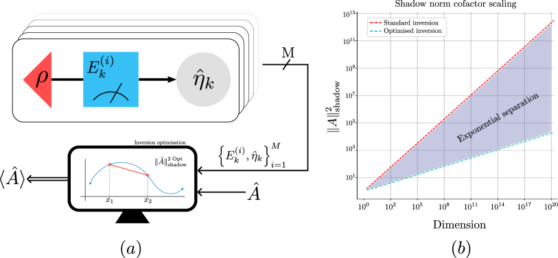
Figure 1: (a) Classical shadow tomography with optimised shadow inversion. After a collection of $M$ POVM outcomes have been acquired from a fixed quantum state, any estimation can be improved for a dynamic choice of target observable $A$ by computing an optimal ‘inverse’ operation for that observable and POVM. (b) Shadow norm for different strategies. The shadow norm cofactor when optimised for certain target projectors, using local Pauli measurements on single qubits. The shadow norm for such an observable on $N$ qubits is normally $(3/2)^{N}$ but when optimised over additional degrees of freedom can be shrunk to $(1.15)^{N}$. Though still exponential in the number of qubits, the optimised strategy is exponentially cheaper than standard classical shadow tomography with local measurements.

In these cases, the inversion map takes a particularly simple form, and the estimation of consumed resources (sampling complexity) critically depends on it. Nevertheless, what is often neglected in studies is the fact that such a map is not unique, i.e., as long as the POVM used is overcomplete (in the operator, Hilbert-Schmidt space), an additional set of free parameters appear in the inversion process which may be optimised to improve the post-processing performance of the estimation procedure. Surprisingly, this has been only recently recognised in the literature Innocenti et al. (2023) by employing the techniques of measurement dual frames. In this work, we demonstrate that such additional degrees of freedom reside in the homogeneous space, i.e. the general inverse map contains a free homogeneous component $\mathcal{M}^{-1}=\mathcal{M}_{p}^{-1}+\mathcal{M}_{h}^{-1}$ which can be further optimized. Our goal is to pursue such an optimisation by considering a hereto before missed resource in the tomography procedure that appears most vividly in classical shadows and the post-processing thereof. Though the natural choice of the inverse map (such as the one given above) is the inverse of the forward channel being applied, there is nothing that says it must be so. It is this inversion process, normally treated as a fixed mathematical procedure, that we aim to modify and improve upon. As long as the set of performed measurements is tomographically over-complete, the additional degrees of freedom may be exploited to reduce case-specific variance for a given observable. In doing so, we will show that an exponential improvement in estimations is possible compared to the standard choice of inverse map presented in the literature. With this novel approach to processing acquired quantum data, we open a new route to exploit areas where advantages may be gained without incurring an unacceptable resource cost.

Shadow map inversion

We begin by describing a generalised procedure Morris and Dakić (2020); Nguyen et al. (2022), depicted in Figure 1(a) fulfilling the random measurement scheme with a fixed POVM $\{E_{k}\}_{k=1}^{n}$ on a $d$-dimensional system. The POVM elements sample randomly an unknown state $\rho$ with probability $p_{k}=\mbox{Tr}\left[{\rho E_{k}}\right]$. These POVM elements span a subspace $\mathcal{V}_{D}=\mathrm{Span}\{E_{k}\}_{k=1}^{n}$ in the Hilbert-Schmidt space (HS) of the dimension $|\mathcal{V}_{D}|=D$. Typically, $D=d^{2}$ (the entire HS space), but for the sake of generality, we shall keep $D\leq d^{2}$. Furthermore, we assume $D<n$, thus $E_{k}$ forms an over-complete basis in $\mathcal{V}_{D}$. The estimation task aims to approximate the mean values of an observable $A\in\mathcal{V}_{D}$, i.e., $\expectationvalue{A}=\mbox{Tr}\left[{A\rho}\right]$. Note that $\expectationvalue{A}=\mbox{Tr}\left[{A\bar{\rho}}\right]$, with $\bar{\rho}$ being the projection of a quantum state $\rho$ onto $\mathcal{V}_{D}$ which follows directly from $A\in\mathcal{V}_{D}$. For the case of the entire HS space, we have $\bar{\rho}=\rho$. Similarly, the measured probabilities trivially satisfy $p_{k}=\mbox{Tr}\left[{E_{k}\rho}\right]=\mbox{Tr}\left[{E_{k}\bar{\rho}}\right]$. The post-processing task assigns a (matrix) estimator $\hat{\eta}\in\{\dots,\hat{\eta}_{k},\dots\}$, i.e. each outcome $E_{k}$ the corresponding matrix $\hat{\eta}_{k}$, which represents a single-shot approximation of $\bar{\rho}$. They can be calculated via an inversion map $\hat{\eta_{k}}=\mathcal{M}^{-1}(E_{k})$ Huang et al. (2020); Nguyen et al. (2022) which we will show is not unique, i.e. $\mathcal{M}^{-1}=\mathcal{M}_{p}^{-1}+\mathcal{M}_{h}^{-1}$ with the latter (homogeneous) component containing auxiliary parameters that may be used as a free resource in post-processing.

The overall classical shadow itself is obtained by averaging over the estimators obtained from $M$ random measurements: $M^{-1}\sum_{s}^{M}\hat{\eta}^{(s)}$. Assuming that all samples are i.i.d., the average value $\expectationvalue{\hat{\eta}}$ is immediately

$$\expectationvalue{\hat{\eta}}=\sum_{k=1}^{n}p_{k}\hat{\eta}_{k}=\sum_{k=1}^{n}\mbox{Tr}\left[{\bar{\rho}E_{k}}\right]\hat{\eta}_{k}\overset{!}{=}\bar{\rho},~{}~{}~{}\forall\bar{\rho}\in\mathcal{V}_{D}.$$ (3)

This is the requirement on the estimator $\hat{\eta}$ such that the statistics of the shadow mimics, in expectation, that of the actual unknown state. Since the POVM forms an over-complete basis in $\mathcal{V}_{D}$, any solution to Eq. (3) is not unique. This multiplicity results in a set of free parameters, which becomes an extra resource that may be used in the post-processing component of an estimation to reduce the variance.

To achieve this, we now show a constructive method to recover families of equivalent classical shadows in terms of the POVM elements and their free parameters. We rely on an equivalent problem to (3), that is, to impose the equivalence between the expectation value of an observable $A$ and the corresponding classical estimator $a=\mbox{Tr}\left[{A\hat{\eta}}\right]$:

$$\expectationvalue{\,a\,}=\mbox{Tr}\left[{A\expectationvalue{\hat{\eta}}}\right]=\sum_{k=1}^{n}p_{k}\mbox{Tr}\left[{A\,\hat{\eta}_{k}}\right]\overset{!}{=}\mbox{Tr}\left[{\bar{\rho}A}\right].$$ (4)

It is instructive to express the operators as vectors in $\mathcal{V}_{D}$, i.e., for an operator $X\in\mathcal{V}_{D}$, we shall use the ket notation $|{X}\rangle\!\rangle$. We also identify an orthonormal basis $\beta_{D}=\{|{B_{j}}\rangle\!\rangle\}_{j=1}^{D}$ in $\mathcal{V}_{D}$. The expectation value from (4) can be expressed as

$$\expectationvalue{\,a\,}=\sum_{k=1}^{n}\langle\!\langle{A^{\dagger}}|{\eta_{k}}\rangle\!\rangle\langle\!\langle{E_{k}^{\dagger}}|{\rho}\rangle\!\rangle\overset{!}{=}\langle\!\langle{A^{\dagger}}|{\bar{\rho}}\rangle\!\rangle$$ (5)

where $\langle\!\langle{X}|{Y}\rangle\!\rangle=\mbox{Tr}\left[{X^{\dagger}Y}\right]$. To guarantee the estimators are unbiased, the requirement reduces to a resolution of the identity in the subspace $\mathcal{V}_{D}$

$$\sum_{k=1}^{n}|{\eta_{k}}\rangle\!\rangle\langle\!\langle{E_{k}^{\dagger}}|=\sum_{k=1}^{n}|{\eta_{k}}\rangle\!\rangle\langle\!\langle{E_{k}}|\equiv\mathbbm{1}_{D},$$ (6)

which can be solved for $|{\eta_{k}}\rangle\!\rangle$ using $E_{k}^{\dagger}=E_{k}$. The last equation expressed in the basis $\beta_{D}$ reads

$$\sum_{k=1}^{n}\langle\!\langle{B_{s}}|{\hat{\eta}_{k}}\rangle\!\rangle\langle\!\langle{E_{k}}|{B_{t}}\rangle\!\rangle=\sum_{k=1}^{n}L_{sk}R_{tk}^{*}\overset{!}{=}\delta_{st},$$ (7)

with $L_{sk}=\langle\!\langle{B_{s}}|{\hat{\eta}_{k}}\rangle\!\rangle$ and $R_{tk}=\langle\!\langle{B_{t}}|{E_{k}}\rangle\!\rangle$. This implies the matrix equation $LR^{\dagger}=\mathbbm{1}_{D}$; thus, $L$ is a generalised inverse of $R^{\dagger}$. Since $R$ is a $D\times n$ matrix having $|{E_{k}}\rangle\!\rangle$ as columns, it is a rank-$D$ matrix (recall there are only $D$ independent $E_{k}$ matrices). We can write its singular value decomposition (SVD), i.e., $R=U(\Sigma|\hat{0})W^{\dagger}$ with $\Sigma=\mathrm{diag}[\sigma_{1},\dots,\sigma_{D}]$ ($\sigma_{s}>0$) and $\hat{0}$ being the $D\times(n-D)$ zero-matrix. Having this, a simple exercise shows $L=W(\Sigma^{-1}|H)U^{\dagger}$ with $H$ being an arbitrary $D\times(n-D)$ matrix. Accordingly, we can split solution into two parts $L=L^{(p)}+L^{(h)}$, with $L^{(p)}=W(\Sigma^{-1}|\hat{0})U^{\dagger}$ (particular) and $L^{(h)}=W(\hat{0}|H)U^{\dagger}$ (homogeneous). This results in a family of equivalent estimators

$$\hat{\eta_{k}}=\sum_{s=1}^{D}L_{sk}\hat{B_{s}}=\sum_{s=1}^{D}\left(L_{sk}^{(p)}+L_{sk}^{(h)}\right)\hat{B_{s}}=\hat{\eta}_{k}^{(p)}+\hat{\eta}_{k}^{(h)},$$ (8)

parameterised by a homogeneous solution $\hat{\eta}_{k}^{(h)}$. As we shall see, this multiplicity of possible inversion schemes represents an additional resource for error optimisation in post-processing. We turn to observable properties which may be expressed in terms of estimator coefficients $a_{k}=\mbox{Tr}\left[{A\hat{\eta}_{k}}\right]=a_{k}^{(p)}+a_{k}^{(h)}$, with $a_{k}^{(p/h)}=\mbox{Tr}\left[{A\hat{\eta}_{k}^{(p/h)}}\right]$ where the homogeneous coefficients do not influence expectation values or any other linear combination of classical shadows

$$\expectationvalue{\,a\,}=\sum_{k=1}^{n}p_{k}a_{k}=\sum_{k=1}^{n}p_{k}\left(a_{k}^{(p)}+a_{k}^{(h)}\right)=\sum_{k=1}^{n}p_{k}a_{k}^{(p)}.$$ (9)

By substituting $p_{k}=\mbox{Tr}\left[{\rho E_{k}}\right]$ and $\expectationvalue{\,a\,}=\mbox{Tr}\left[{AE_{k}}\right]$ into the previous equation we find

$$\sum_{k}a_{k}^{(p)}E_{k}=A,$$ (10)

$$\sum_{k}a_{k}^{(h)}E_{k}=0.$$ (11)

The set of solutions to the latter (homogeneous) equation defines an auxiliary optimisation space of dimension $n-D$ independent of the target observable (fixed by the choice of POVM). This is a free resource that may now be used in post-processing.

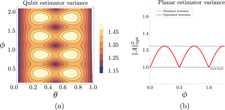
Figure 2: (a) Optimal free parameter for projectors on the Bloch sphere. The contour plot shows the minimal shadow norm (13) of the single-qubit projector characterised by the Bloch sphere angles $\theta,\,\phi$ (in units of $\pi$). Optimisation results in bounds lower or equal than $3/2$, obtained via the Clifford inversion map (15) found in Huang et al. (2020) (b) Optimal free parameter for plane projectors. The optimal value of the shadow norm of the single-qubit projector in the equatorial plane in terms of a single angle parameter $\phi$ (in units of $\pi$). This enhanced norm is always lower or equal to the standard shadow norm $\|\outerproduct{\psi}{\psi}(\phi)\|^{2}_{\text{sh}}\leq 5/4$ (see main text). In the case of $\phi=k\frac{\pi}{2},\,k\in\mathbb{Z}$, which corresponds to the projectors on the Pauli $X$ and $Y$ basis. The bound corresponds to the combinations which present optimal variance $\|\outerproduct{\psi}{\psi}(\phi)\|^{2}_{\text{sh}}\equiv 1$.

Now, to effectively compare the different choices for estimators, we refer to the efficiency of the estimation process, that is the expected sample size of copies required to estimate a property of the state up to a fixed accuracy. It is customary in classical shadow tomography to refer to variance as figure of merit Huang et al. (2020). In particular, we consider the state-independent upper bound on variance, defined as the shadow norm, which only depends on the decomposition of the particular observable:

$$\mbox{Var}\left[{a}\right]\leq\max_{\sigma:\text{state}}\mbox{Tr}\left[{\sigma\sum_{k=1}^{n}|a_{k}^{(p)}+a_{k}^{(h)}|^{2}E_{k}}\right]=\|A\|^{2}_{\text{shadow}}.$$ (12)

This quantity is equivalent to the maximal eigenvalue of the variance operator defined as $\hat{O}_{A}\coloneq\sum_{k=1}^{n}|a_{k}^{(p)}+a_{k}^{(h)}|^{2}E_{k}$; we will use both definitions interchangeably. This is akin to the original upper bound on shadow norm and thence sampling complexity found in Huang et al. (2020), where the expected number of samples scales with $M=O(\varepsilon^{-2}\log{\delta^{-1}}\|A\|^{2}_{\text{shadow}})$. Nevertheless, this can be further optimised over the free parameters in the homogeneous part of the estimator. By optimising over these coefficients, it is possible to identify the configuration which guarantees the minimal sample size for the estimation of the particular observable $A$:

$$\|A\|^{2}_{\text{opt}}=\min_{a_{k}^{(h)}:H}\max_{\sigma:\text{state}}\mbox{Tr}\left[{\sigma\sum_{k=1}^{n}|a_{k}^{(p)}+a_{k}^{(h)}|^{2}E_{k}}\right],$$ (13)

The existence of a minimum is guaranteed through the positive semidefiniteness of the variance operator. We will provide examples to illustrate that different choices of free parameters may result in a sampling complexity with exponential separation compared to that of the naive estimator construction, which shows, in turn, that optimisation in (13) yields exceptional gains for relatively minuscule cost.

Product observables and shadow optimisation

Let us now discuss the estimation of product observables $A^{(N)}=A_{1}\otimes A_{2}\ldots\otimes A_{N}$ via local POVMs, i.e., of the type $E_{k_{1}}\otimes\dots\otimes E_{k_{n}}$. This case is particularly interesting for near-term applications, such as the VQE algorithm Peruzzo et al. (2014); Tilly et al. (2022). In such a scenario, it is easy to show that the shadow norm in Eq. (12) has a product form (see also Nguyen et al. (2022)) and consequently Eq. (13) becomes

$$\|A^{(N)}\|^{2}_{\text{opt}}=\prod_{j=1}^{N}\|A_{j}\|^{2}_{\text{opt}}$$ (14)

The optimisation in Eq. (12) appears efficient, given the total number of free parameters scales linearly with the number of subsystems $N$. We see that even minimal deviation from the minimum in local shadow norms $\|A_{j}\|^{2}_{\text{opt}}$ may accumulate exponentially fast with $N$. This is illustrated in Figure 1(b) for the case of the canonical inversion map of Eq. (15). We now present examples of such exponential improvement for qubits for particular sets of local observables, specifically projectors, whereby by adjusting the available free parameters, we are able to reduce the expected bound on sample size based on assumptions for the observable itself.

Fidelity estimation of product states

We first consider the case of estimation of fidelity with product states. The target observables are thus tensor products of a projector on a single qubit $\bigotimes_{j=1}^{N}\outerproduct{\psi_{j}}{\psi_{j}}$, parameterised on the Bloch sphere by two angles $(\theta_{j},\,\phi_{j})$. The measurement scheme is described by the POVM of projectors on the Pauli basis $E^{\pm}_{\zeta}=\frac{1}{2}(\mathbbm{1}\pm\sigma_{\zeta})$, where $\zeta=x,\,y,\,z$. As reference, we consider the bound $\|\bigotimes_{j=1}^{N}\outerproduct{\psi_{j}}{\psi_{j}}\|^{2}_{\text{shadow}}\equiv(3/2)^{N}$ obtained using the estimators

$$\hat{\eta}^{\pm}_{\zeta}=3\left(3E^{\pm}_{\zeta}-\mbox{Tr}\left[{E^{\pm}_{\zeta}}\right]\mathbbm{1}_{3}\right).$$ (15)

found in Huang et al. (2020). Now we show how to improve this bound by our techniques. The POVMs $E^{\pm}_{\zeta}$ span the entire HS space. We have $n=6$ and $D=4$, thus the equation (11) gives two free optimisation parameters for each qubit See supplementary material at [URL from publisher] for information concerning estimator explicit parameter dependence . In Fig.2(a), we present the minimal upper bound as a function of angles $(\theta,\phi)$, which is contained within the interval $1.15\leq\|\outerproduct{\psi_{j}}{\psi_{j}}\|^{2}_{\text{sh}}\leq 1.5$. Since the overall shadow norm (14) is of the product form, there are entire regions in the $(\theta,\phi)$-space for which deviations from from the standard $3/2$ leads to the exponential improvement in $N$.

Locally efficient fidelity estimation implies globally efficient

We now present a configuration in which the optimisation of the inversion map not only improves the standard bound, but we are actually able to achieve efficiency, i.e. $\|A\|^{2}_{\text{opt}}\equiv 1$. We consider the POVM constituted by the projectors of the X and Y Paulis, which spans the ”equator” on the Bloch sphere. The target observables are tensor products of a projector on a single qubit, parameterised by a single angle: $A=\outerproduct{\psi(\phi)}{\psi(\phi)}$ with $|{\psi(\phi)}\rangle=(|{0}\rangle+e^{i\phi}|{1}\rangle)\sqrt{2}$. As before, we follow the ansatz given in Huang et al. (2020) to get the particular solution for the inversion map and estimators

$$\hat{\eta}^{\pm}_{\zeta}=4E^{\pm}_{\zeta}-\mbox{Tr}\left[{E^{\pm}_{\zeta}}\right]\mathbbm{1}_{2}.$$ (16)

From here we obtain the reference bound for the shadow norm of $\|\bigotimes_{j=1}^{N}\outerproduct{\psi_{j}}{\psi_{j}}\|^{2}_{\text{sh}}\equiv(5/4)^{N}$. We reference to Supplementary Information See supplementary material at [URL from publisher] for information concerning shadow norm expression for local Clifford measurements for more precise remarks on how we obtain this result.

Now we turn to our optimisation technique. We have the POVM with $n=4$ elements spanning a subspace of dimension $D=3$, therefore the generic estimators obtained from our procedure depend on a single free parameter $p$. The shadow norm of single-qubit projector depends on this free parameter and on the angle parameter $\phi$:

$$\|\outerproduct{\psi}{\psi}(\phi)\|^{2}_{\text{sh}}=\frac{1}{2} (1+p_{i}^{2}+B(\phi,p_{r})+$$ (17)

$$\quad\sqrt{2}\sqrt{C(\phi,p_{r})})$$

$$B(\phi,p_{r})=(4 p_{r}-2)\cos{\phi}+\cos{2\phi}+2$$ (18)

$$\quad+2p_{r}(p_{r}-1)$$

$$C(\phi,p_{r})=(4 p_{r}-1)\cos{\phi}+2p_{r}\cos{2\phi}$$ (19)

$$\quad+\cos{3\phi}+2+2p_{r}(p_{r}-1),$$

where $p_{r}=\Re{p},\,p_{i}=\Im{p}$.

In general, the dependency on $\phi$ remains explicit, changing the expected bound based on the projector to be estimated. In Fig.2(b) we present the optimal value of the shadow norm for each parameter $\phi\in[0,\pi]$. We note that for each value of $\phi$ the optimised norm is $\|\outerproduct{\psi}{\psi}(\phi)\|^{2}_{\text{opt}}\leq 5/4$. Moreover, it can be seen that for specific angles, the bound is exactly $\|E_{\zeta}^{\pm}\|^{2}_{\text{opt}}\equiv 1$., i.e., for the eigenprojectors of $X$ and $Y$ Paulis, corresponding to the POVM elements themselves. This implies efficient estimation: given the product form of the overall shadow norm (14), this scaling represents not only an exponential improvement compared to $(5/4)^{N}$, as for other projectors, but also an expected constant scaling of the sample size with the number of qubits. This is particularly relevant considering that X and Y are non-commuting observables, as it opens the possibility of the simultaneous estimation of up to $2^{N}$ projections simultaneously for complementary observables. Previously this result has been found only via global measurement strategies relying on Clifford unitaries consisting of many joint operations, acting on all $N$ qubits at the same time; we have shown instead that by introducing the initial assumption over the space of observables, this could be achieved using only local single-qubit measurements.

Discussion

In the course of this letter we have observed how post-processing, an often overlooked aspect in estimation, represents a relevant resource to be examined in the accounting of a more efficient tomography. By introducing a generalised framework to obtain families of equivalent parameter-dependent estimators, we have found a clear relation between over-complete POVMs and their ability to reduce the variance in estimation of arbitrary observables. When considering local measurements on large composite quantum systems, even a small gain on each estimator represents an overall improvement in sample complexity, yielding an exponential separation between the naive sample variance and the optimised one as seen in Figure 1(b). In the case of example two, this optimised gain can achieve a variance that performs as well as global classical shadows for given observables, with modest additional post processing that remains efficient. We anticipate that by considering overcomplete POVMs containing joint measurements on multiple qubits, further advantage may be found at increased (but still tractable) optimisation difficulty, either in sample complexity or the set of observables. Finally, interleaving optimised multiqubit measurements may yield sample improvements that approach regular classical shadows within some limit. Such questions are natural candidates for further investigation and the identification of such a hierarchy of optimisation will be the topic of future work.

Note - In preparation of this manuscript, we became aware of two other works Malmi et al. (2024); Fischer et al. (2024) considering a similar problem. The authors consider a similar optimisation of the post-processing stage in estimation tasks, albeit referring to different frameworks.

Appendix A Parameter dependence for estimators

The POVM of projectors on the Pauli basis $E^{\pm}_{\zeta}=\frac{1}{2}\left(\mathbbm{1}\pm\sigma_{\zeta}\right)$, where $\zeta=x,y,z$, admits a homogeneous combination $\sum_{i=\pm}\sum_{\zeta}h_{i,\zeta}E^{i}_{\zeta}=0$ (see discussion around (11) in the main text) determined by $n=6$ coefficients; given the symmetry of the system, they reduce to $3$ since $h_{\zeta}^{+}=h_{\zeta}^{-}$:

$$\{h_{i,\zeta}\}_{\zeta=x,y,z}=\{h_{\zeta}\}_{\zeta=x,y,z}=\{p_{1},p_{2},-p_{1}-p_{2}\}$$ (20)

A expected, we find $n-D=2$ parameters $p_{1},p_{2}$ which are used to optimise the shadow norm in (14). For the particular solution (see discussion around (10)) of $\sum_{i=\pm}\sum_{\zeta}q_{i,\zeta}E^{i}_{\zeta}=A=a\mathbbm{1}+\sum_{\zeta=x,y,z}\zeta\sigma_{\zeta}$ we can obtain the particular coefficients

$$q_{\pm,\zeta}=a\pm 3\zeta$$ (21)

where $\zeta=x,y,z$. In order to find the expression for the generic projector $\outerproduct{\psi}{\psi}(\theta,\phi)$, one can simply rely on the parametrisation $a\to\frac{1}{2}$, $x\to\frac{1}{2}\sin\theta\cos\phi$, $y\to\frac{1}{2}\sin\theta\sin\phi$, $z\to\frac{1}{2}\cos\theta$. This particular solution corresponds to the coefficients found with the estimators obtained with the standard inversion map, as introduced in B.0.1.

Appendix B Shadow norm expression for local Clifford measurements

In this section, we detail the explicit expressions for the shadow norm obtained using the standard estimators (15), as introduced in the seminal work on Classical Shadows.

B.0.1 Shadow norm for local Pauli measurements

The POVM of projectors on the Pauli basis $E^{\pm}_{\zeta}=\frac{1}{2}\left(\mathbbm{1}\pm\sigma_{\zeta}\right)$, where $\zeta=x,y,z$. For a generic single-qubit observable $A=a\mathbbm{1}+\sum_{\zeta=x,y,z}\zeta\sigma_{\zeta}$ the shadow norm in (12) simply evaluates to

$$\|A\|^{2}_{\text{sh}}=a^{2}+3(x^{2}+y^{2}+z^{2})+2|a|\sqrt{x^{2}+y^{2}+z^{2}}.$$ (22)

Considering the particular case of projectors on the Bloch sphere, with the parameterization $a\to\frac{1}{2}$, $x\to\frac{1}{2}\sin\theta\cos\phi$, $y\to\frac{1}{2}\sin\theta\sin\phi$, $z\to\frac{1}{2}\cos\theta$, (22) trivially reduces to $\|\outerproduct{\psi}{\psi}\|^{2}_{\text{sh}}\equiv\frac{3}{2}$.

B.0.2 Shadow norm for local Pauli measurements on the plane

In this simplified case, the set of POVMs spend a subspace on the equatorial plane of the Bloch sphere, i.e., $\mathcal{V}_{D=3}=\mathrm{span}\{\mathbbm{1},X,Y\}$. The generic target observable can be thus represented as

$$A=\spmqty{undef}.$$ (23)

As a reference, we use the ansatz from Huang et al. (2020) to find the inversion map in the form

$$\hat{\eta}_{k}=\mathcal{M}^{-1}[E_{k}]=\mathcal{N}(\lambda E_{k}-\mu\,\mbox{Tr}\left[{E_{k}}\right]\mathbbm{1}_{2}).$$ (24)

A simple inspection shows $\mathcal{N}=2$, $\lambda=2$ and $\mu=\frac{1}{2}$. The shadow norm of the generic observable results as

$$\|A\|^{2}_{\text{sh}}=a^{2}+2(x^{2}+y^{2})+2|a|\sqrt{x^{2}+y^{2}}.$$ (25)

For the case of projectors we have $x\to\cos{\phi}/2$ and $y\to\sin{\phi}/2$, thus we get $\|\outerproduct{\psi(\phi)}{\psi(\phi)}\|^{2}_{\text{sh}}\equiv\frac{5}{4}$.

References

- Huang et al. (2020) H.-Y. Huang, R. Kueng, and J. Preskill, Nature Physics 16, 1050–1057 (2020).
- Aaronson (2017) S. Aaronson, (2017), 10.48550/ARXIV.1711.01053.
- Hu et al. (2023) H.-Y. Hu, S. Choi, and Y.-Z. You, Phys. Rev. Res. 5, 023027 (2023).
- Elben et al. (2020) A. Elben, R. Kueng, H.-Y. R. Huang, R. van Bijnen, C. Kokail, M. Dalmonte, P. Calabrese, B. Kraus, J. Preskill, P. Zoller, and B. Vermersch, Phys. Rev. Lett. 125, 200501 (2020).
- Huang et al. (2021) H.-Y. Huang, R. Kueng, and J. Preskill, Phys. Rev. Lett. 127, 030503 (2021).
- Neven et al. (2021) A. Neven, J. Carrasco, V. Vitale, C. Kokail, A. Elben, M. Dalmonte, P. Calabrese, P. Zoller, B. Vermersch, R. Kueng, and B. Kraus, npj Quantum Information 7, 152 (2021).
- Crawford et al. (2021) O. Crawford, B. v. Straaten, D. Wang, T. Parks, E. Campbell, and S. Brierley, Quantum 5, 385 (2021).
- Chen et al. (2021) S. Chen, W. Yu, P. Zeng, and S. T. Flammia, PRX Quantum 2, 030348 (2021).
- Hadfield et al. (2022) C. Hadfield, S. Bravyi, R. Raymond, and A. Mezzacapo, Communications in Mathematical Physics 391, 951 (2022).
- Zhao et al. (2021) A. Zhao, N. C. Rubin, and A. Miyake, Phys. Rev. Lett. 127, 110504 (2021).
- Seif et al. (2023) A. Seif, Z.-P. Cian, S. Zhou, S. Chen, and L. Jiang, PRX Quantum 4, 010303 (2023).
- Wan et al. (2023) K. Wan, W. J. Huggins, J. Lee, and R. Babbush, Communications in Mathematical Physics 404, 629 (2023).
- Levy et al. (2024) R. Levy, D. Luo, and B. K. Clark, Phys. Rev. Res. 6, 013029 (2024).
- Bu et al. (2024) K. Bu, D. E. Koh, R. J. Garcia, and A. Jaffe, npj Quantum Information 10, 6 (2024).
- Coopmans et al. (2023) L. Coopmans, Y. Kikuchi, and M. Benedetti, PRX Quantum 4, 010305 (2023).
- Bertoni et al. (2023) C. Bertoni, J. Haferkamp, M. Hinsche, M. Ioannou, J. Eisert, and H. Pashayan, (2023), arXiv:2209.12924 [quant-ph] .
- Koh and Grewal (2022) D. E. Koh and S. Grewal, Quantum 6, 776 (2022).
- McGinley and Fava (2023) M. McGinley and M. Fava, Phys. Rev. Lett. 131, 160601 (2023).
- Kunjummen et al. (2023) J. Kunjummen, M. C. Tran, D. Carney, and J. M. Taylor, Phys. Rev. A 107, 042403 (2023).
- Iosue et al. (2024) J. T. Iosue, K. Sharma, M. J. Gullans, and V. V. Albert, Phys. Rev. X 14, 011013 (2024).
- Nakaji et al. (2023) K. Nakaji, S. Endo, Y. Matsuzaki, and H. Hakoshima, Quantum 7, 995 (2023).
- Feldman et al. (2022) N. Feldman, A. Kshetrimayum, J. Eisert, and M. Goldstein, PRX Quantum 3, 030312 (2022).
- Wyderka et al. (2023) N. Wyderka, A. Ketterer, S. Imai, J. L. Bönsel, D. E. Jones, B. T. Kirby, X.-D. Yu, and O. Gühne, Phys. Rev. Lett. 131, 090201 (2023).
- Sack et al. (2022) S. H. Sack, R. A. Medina, A. A. Michailidis, R. Kueng, and M. Serbyn, PRX Quantum 3, 020365 (2022).
- Anshu et al. (2021) A. Anshu, S. Arunachalam, T. Kuwahara, and M. Soleimanifar, Nature Physics 17, 931 (2021).
- Huang et al. (2023) H.-Y. Huang, S. Chen, and J. Preskill, PRX Quantum 4, 040337 (2023).
- Nguyen et al. (2022) H. C. Nguyen, J. L. Bönsel, J. Steinberg, and O. Gühne, Phys. Rev. Lett. 129, 220502 (2022).
- Zhang et al. (2021) T. Zhang, J. Sun, X.-X. Fang, X.-M. Zhang, X. Yuan, and H. Lu, Phys. Rev. Lett. 127, 200501 (2021).
- Struchalin et al. (2021) G. Struchalin, Y. A. Zagorovskii, E. Kovlakov, S. Straupe, and S. Kulik, PRX Quantum 2, 010307 (2021).
- Stilck França et al. (2024) D. Stilck França, L. Markovich, V. Dobrovitski, A. Werner, and J. Borregaard, Nat Commun. 15 (2024), doi: 10.1038/s41467-023-44012-5.
- Ippoliti et al. (2023) M. Ippoliti, Y. Li, T. Rakovszky, and V. Khemani, Phys. Rev. Lett. 130, 230403 (2023).
- Morris et al. (2022) J. Morris, V. Saggio, A. Gočanin, and B. Dakić, Advanced Quantum Technologies 5, 2100118 (2022), https://onlinelibrary.wiley.com/doi/pdf/10.1002/qute.202100118 .
- Glos et al. (2022) A. Glos, A. Nykänen, E.-M. Borrelli, S. Maniscalco, M. A. C. Rossi, Z. Zimborás, and G. García-Pérez, (2022), arXiv:2208.07817 [quant-ph] .
- Stricker et al. (2022) R. Stricker, M. Meth, L. Postler, C. Edmunds, C. Ferrie, R. Blatt, P. Schindler, T. Monz, R. Kueng, and M. Ringbauer, PRX Quantum 3, 040310 (2022).
- Vermersch et al. (2023) B. Vermersch, M. Ljubotina, J. I. Cirac, P. Zoller, M. Serbyn, and L. Piroli, (2023), arXiv:2311.08108 [quant-ph] .
- Huang et al. (2022) H.-Y. Huang, M. Broughton, J. Cotler, S. Chen, J. Li, M. Mohseni, H. Neven, R. Babbush, R. Kueng, J. Preskill, and J. R. McClean, Science 376, 1182 (2022), https://www.science.org/doi/pdf/10.1126/science.abn7293 .
- García-Pérez et al. (2021) G. García-Pérez, M. A. Rossi, B. Sokolov, F. Tacchino, P. K. Barkoutsos, G. Mazzola, I. Tavernelli, and S. Maniscalco, PRX Quantum 2, 040342 (2021).
- Webb (2016) Z. Webb, (2016), arXiv:1510.02769 [quant-ph] .
- Zhu (2017) H. Zhu, Phys. Rev. A 96, 062336 (2017).
- Innocenti et al. (2023) L. Innocenti, S. Lorenzo, I. Palmisano, F. Albarelli, A. Ferraro, M. Paternostro, and G. M. Palma, PRX Quantum 4, 040328 (2023).
- Morris and Dakić (2020) J. Morris and B. Dakić, (2020), arXiv:1909.05880 [quant-ph] .
- Peruzzo et al. (2014) A. Peruzzo, J. McClean, P. Shadbolt, M.-H. Yung, X.-Q. Zhou, P. J. Love, A. Aspuru-Guzik, and J. L. O’Brien, Nature Communications 5 (2014), 10.1038/ncomms5213.
- Tilly et al. (2022) J. Tilly, H. Chen, S. Cao, D. Picozzi, K. Setia, Y. Li, E. Grant, L. Wossnig, I. Rungger, G. H. Booth, and J. Tennyson, Physics Reports 986, 1–128 (2022).
- (44) See supplementary material at [URL from publisher] for information concerning estimator explicit parameter dependence, .
- (45) See supplementary material at [URL from publisher] for information concerning shadow norm expression for local Clifford measurements, .
- Malmi et al. (2024) J. Malmi, K. Korhonen, D. Cavalcanti, and G. García-Pérez, (2024), arXiv:2401.18049 [quant-ph] .
- Fischer et al. (2024) L. E. Fischer, T. Dao, I. Tavernelli, and F. Tacchino, (2024), arXiv:2401.18071 [quant-ph] .