Value-based Resource Matching with Fairness Criteria: Application to Agricultural Water Trading

Abstract.

Optimal allocation of agricultural water in the event of droughts is an important global problem. In addressing this problem, many aspects, including the welfare of farmers, the economy, and the environment, must be considered. Under this backdrop, our work focuses on several resource-matching problems accounting for agents with multi-crop portfolios, geographic constraints, and fairness. First, we address a matching problem where the goal is to maximize a welfare function in two-sided markets where buyers’ requirements and sellers’ supplies are represented by value functions that assign prices (or costs) to specified volumes of water. For the setting where the value functions satisfy certain monotonicity properties, we present an efficient algorithm that maximizes a social welfare function. When there are minimum water requirement constraints, we present a randomized algorithm which ensures that the constraints are satisfied in expectation. For a single seller–multiple buyers setting with fairness constraints, we design an efficient algorithm that maximizes the minimum level of satisfaction of any buyer. We also present computational complexity results that highlight the limits on the generalizability of our results. We evaluate the algorithms developed in our work with experiments on both real-world and synthetic data sets with respect to drought severity, value functions, and seniority of agents.

1. Introduction

1.1. Background

The growth in the global population has led to a significant increase in demand for agricultural and urban water supplies Food and Organization (2022). However, water supply augmentation has reached its limit Chong and Sunding (2006). Furthermore, climate change has led to an increased occurrence of droughts, which, in turn, lead to severe water shortages Kallis (2008). Water markets have been widely proposed as an effective means of water reallocation during such shortages Chong and Sunding (2006), and several formal and informal markets have emerged across the world Wheeler (2021); Howe (2013); Howe and Goemans (2003). A widely proposed (but much debated) approach is socially optimal water allocation, where water is transferred from low-value to high-value agricultural applications Chong and Sunding (2006); Howe (2013); Xu et al. (2018). Much of the work in this regard has focused on elaborate modeling of agricultural, hydrological and economic aspects of the problem as explored through complex agent-based models (see, e.g., Raffensperger et al. (2009); Raffensperger and Milke (2017); Basu (2023); Sharghi and Kerachian (2022)). Some references have addressed computational aspects of such models (see, e.g., Liu et al. (2016); Li et al. (2017)).

While our work is applicable to many water market settings, it is motivated by the river water allocation mechanisms for agriculture in the western US Brajer et al. (1989); Leonard et al. (2019); Booker and Young (1994). Here, water is allocated according to the prior appropriation doctrine, which induces a seniority ordering among farmers Chong and Sunding (2006); Project (2019). When water is curtailed due to shortages, it is made available to only those water rights holders who are above a seniority threshold chosen by appropriate authorities based on the drought severity. This naturally partitions the set of farmers into two groups: potential sellers and potential buyers, leading to a two-sided market. An example is provided in Figure 1. In addition, there are scenarios involving external entities, such as water aggregators or brokers, who pool water from multiple sellers (see, e.g., Market (2023); Leonard et al. (2019); Selman et al. (2009)) and sell it to buyers.

Under this backdrop, we focus on a class of value-based resource matching problems. We consider a set of agents (farmers), each associated with a discrete ordered set of resources (unit volumes of water, or simply water units). Each water unit is associated with a value, which depends on what use that unit of water is being put to (low-value or high-value crops). Since farmers can have multi-crop portfolios, the value of water units may vary, not only from one agent to another, but also within an agent’s resource set. Broadly, our work is applicable to many market settings that involve multiple identical units of resources, such as financial markets, electricity, CPU job scheduling, and bandwidth allocation Sandholm and Suri (2002); Deng et al. (2007); Khorasany et al. (2020).

In a two-sided market where the agents are partitioned into sellers and buyers by seniority, a seller’s value for a water unit can be considered the minimum price the seller is willing to accept, while, for a buyer, it is the maximum price the buyer is willing to pay. Additionally, due to geographic and legal constraints, not every buyer is compatible with a seller for trading water. This relationship is represented by a buyer–seller bipartite compatibility graph; see Figure 1 for an example of stream flow and the resulting compatibility graph. The objective is to obtain a trading assignment, that is, a matching of sellers’ resources with buyers’ needs, subject to compatibility and value constraints. We will assume that the agents are truthful about their valuations. Every trading assignment is assessed by the total social welfare it generates Liu et al. (2016); Xu et al. (2018).

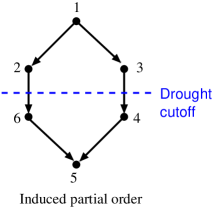
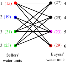
Figure 1. Example. Going from left to right, the first panel shows a sample stream flow and points of diversion for different trading agents. In the second panel, each directed edge $(a,b)$ indicates that $a>b$, that is, $a$ has higher priority than $b$. When there is no directed edge between two nodes, the interpretation is that they belong to different streams. The drought cutoff corresponds to the scenario where water is available to agents $1$, $2$, and $3$. In the compatibility graph shown in the third panel, water units and their values have not yet been factored in. The rightmost panel shows the corresponding resources–needs bipartite graph along with the water units of the buyers and sellers and the corresponding compatibility graph. Here, Seller 3 has, and Buyer 4 needs, two water units, while the others have or need only one water unit each. The values of the water units are shown in parentheses.

1.2. Contributions

Maximizing welfare under monotonicity constraints. We consider the resource matching problem (MaxWelfare), where the goal is to maximize the total welfare. We show that if the value functions satisfy certain monotonicity properties (under the assumption that every agent is rational or profit-maximizing Raffensperger and Milke (2017); Burke et al. (2004); Dang et al. (2016)), an optimal matching can be obtained in polynomial time. We achieve this by transforming the trading assignment problem into the maximum weighted matching problem on a bipartite graph. To complement the above result, we show that MaxWelfare is NP-hard even when the monotonicity constraints are violated only on the buyer’s side.

Maximizing welfare under fairness constraints. We consider the problem (MaxWelfareFair) of maximizing welfare with the additional constraint that, for specified subsets of buyers (where the subsets may also be singletons), a minimum number of water units must be assigned. Such constraints can be viewed as a form of enforcing demographic fairness. In general, we show that the problem of determining whether there is an assignment that satisfies all the lower bound constraints is itself NP-complete. When a solution satisfying all the constraints is known to exist and the value functions satisfy monotonicity properties, we present an efficient randomized algorithm to find a solution that maximizes welfare and satisfies the given lower bound constraints in expectation. To obtain this result, we use the dependent rounding algorithm of Gandhi et al. (2006) and leverage monotonicity properties of value functions.

Maximizing Leximin satisfaction. We consider the special case of a single seller–multiple buyers where each buyer specifies the required number of water units. The satisfaction level of a buyer is the fraction of her requirement that is allocated. We consider the problem where the objective is to find a trading assignment that maximizes the satisfaction level of the least satisfied buyer. We provide an efficient algorithm that finds a valid trading assignment satisfying the following desirable properties: (i) it maximizes the number of resources matched over all valid assignments (thus maximizing seller profit), and (ii) in leximin order Moulin (2004), the vector of buyer satisfaction levels is at least as large as that of any other valid assignment. The use of leximin order as a fairness criterion has also been studied in several other contexts (see, e.g., Chen and Liu (2020); Narang et al. (2022)).

Experiments. We present results from experiments with a class of synthetic data sets and two real-world data sets. The latter correspond to two water basins in the state of Washington, US. We study the impact of factors, such as drought severity, value functions, and farmer seniority, on the compatibility graph structure and objectives of trading assignments (e.g., welfare maximization, maximizing satisfaction levels of buyers). Our results show that the combined effects of seniority, crop profile, and geographic constraints can lead to varied trade outcomes across different datasets.

2. Related work

Many works have proposed mechanisms for optimal matching of buyers to sellers in the context of water markets. Xu et al. Xu et al. (2018) consider a two-sided market with simpler linear value functions where they first apply weighted bipartite matching to achieve welfare maximization. Then, they set transaction prices for each assignment in the matching. In a single-seller/multiple-buyers framework, Raffensperger and Milke Raffensperger et al. (2009); Raffensperger and Milke (2017) use a multipart bidding framework where a buyer’s willingness to pay is modeled as a monotone non-increasing function of the volume of water traded. They develop a linear programming formulation that maximizes the consumer surplus. Using a similar framework but accounting for water quality, Sharghi and Kerachian Sharghi and Kerachian (2022) propose a multi-agent optimization model. Noori et al. Noori et al. (2021) incorporate fairness criteria into their models by requiring that each buyer should receive a certain minimum amount of water depending on the buyer’s demand. The above papers typically also account for a variety of agricultural and socio-economic factors, resulting in very complex optimization problems that are solved using heuristics. As mentioned earlier, our work is applicable to settings that involve indistinguishable units of a resource. In such a setting, Sandholm and Suri Sandholm and Suri (2002) consider the problem of optimal clearing where sellers and buyers specify bids through supply and demand curves.

To our knowledge, very few papers have addressed computational aspects of water markets. Liu et al. Liu et al. (2016) consider the problem of optimal trading assignments in water right markets. They consider two maximization objectives–social welfare and flow–with a minimum threshold constraint on the volume of water traded in each transaction. They consider a setting with linear value functions, where the problem of maximizing welfare can be viewed as maximizing flows in a weighted seller–buyer bipartite graph. Li et al. Li et al. (2017) consider the same setting and examine the assignment problem from the perspective of cooperative game theory. Both works present experimental results using water market data.

Our work is also related to resource allocation problems that are modeled as multi-round matchings Trabelsi et al. (2023) and repeated matchings Caragiannis and Narang (2023). In both cases, the problem can be viewed as a matching (or a $b$-matching) problem Lovász and Plummer (1986) on a bipartite graph, with multiple copies of nodes corresponding to each resource or agent. This is similar to our work, where the water units corresponding to each seller or buyer are represented as nodes of a bipartite graph.

Several recent papers have addressed fairness issues in bipartite matching. For example, Lesmana et al. Lesmana et al. (2019) develop an algorithm with provable guarantees for the trade-off between operator benefit (in our case, a single seller) and the minimum satisfaction or utility for the customer (in our case, a buyer). Esmaeili et al. Esmaeili et al. (2023) consider Rawlsian fairness in online bipartite matchings. Methods to achieve group fairness have also been considered in both offline and online versions of the bipartite matching problem Ma et al. (2022); Esmaeili et al. (2023); Panda et al. (2022).

3. Preliminaries

Let $[k]$ denote the set $\{1,2,\ldots,k\}$ and $\mathbb{R}_{\geq 0}$ be the set of nonnegative real numbers.

Agents, resources, and value functions. Let $A=\{a_{1},a_{2},\ldots,a_{N}\}$ denote the set of $N$ agents. The agents are ordered by seniority; $a_{i}$ is senior to $a_{j}$ for any $i>j$. Each agent $a\in A$ is associated with an ordered set $\Gamma_{a}=\{w^{a}_{1},w^{a}_{2},\cdots,w^{a}_{\gamma_{a}}\}$ of  $\gamma_{a}$ resources or water units. The elements of $\Gamma_{a}$ are ordered so that for all $x<y$, water unit $w^{a}_{x}$ must be sold or bought before the water unit $w^{a}_{y}$; we use the notation $w^{a}_{x}\prec{}w^{a}_{y}$ to indicate this ordering. A value function $f_{a}:\Gamma_{a}\rightarrow\mathbb{R}_{\geq 0}$ assigns a nonnegative value $f_{a}(w)$ to each $w\in\Gamma_{a}$. Each water unit of an agent can be considered to be associated with a specific use (e.g., crop type, which field it is applied to in a farm), and its value can correspond to the anticipated profit, its importance to keep the crop alive or healthy, etc. (see, e.g., Raffensperger and Milke (2017)). The example in Figure 1 shows agents with associated resources and value functions.

Buyers, sellers, and trading. Depending on water availability, the agent set $A$ is partitioned into two sets, namely sellers $S$ and buyers $B$. We let $N_{S}=|S|$ and $N_{B}=|B|$. Each seller $s$ has $\gamma_{s}$ water units, which is the agent’s capacity, while each buyer $b$ has a requirement of $\gamma_{b}$ water units. A trading assignment $\mathcal{T}$ consists of a matching of buyer water units with seller water units; it is specified by a set of ordered pairs of the form $(w^{s}_{i},w^{b}_{j})$.

Compatibility. A seller $s$ is compatible with a buyer $b$ if $b$ is allowed to use the water right owned by $s$. This compatibility relationship is determined by geographic factors such as whether they share a common stream and prevailing water laws. This relationship is represented by a seller–buyer (undirected) bipartite compatibility graph $G(S,B,E)$; a seller $s\in S$ is compatible with a buyer $b\in B$ if and only if there is an edge between $s$ and $b$ in $G$. The example in Figure 1 (third panel) shows a compatibility graph induced by the geographic positions of agents and water availability.

Total value and welfare from trade. We assume that every water unit will be used regardless of whether it is traded or not. If a water unit is traded, then it is used by the corresponding buyer; otherwise, it is used by the seller. The value extracted from each water unit will depend on who uses it (the seller or buyer) and how it is used. For example, if a seller’s unit $w^{s}_{i}$ is matched to a buyer’s unit $w^{b}_{j}$, then its new value is $f_{b}(w^{b}_{j})$. The total value before trade is $\sigma_{0}=\sum_{s\in S}\sum_{w\in\Gamma_{s}}f_{s}(w)$. Given a trading assignment $\mathcal{T}$, let $W_{\mathcal{T}}$ denote the set of matched resources of sellers and let $\overline{W_{\mathcal{T}}}$ denote the set of unmatched resources of sellers. The total value for a given trading assignment $\mathcal{T}$ is $\sigma(\mathcal{T})=\sigma_{0}{}+\operatorname{welfare}(\mathcal{T})$ where $\operatorname{welfare}(\mathcal{T})=\sum_{(w^{s}_{i},w^{b}_{j})\in\mathcal{T}}[f_{b}(w^{b}_{j})-f_{s}(w^{s}_{i})].$ Note that the welfare function does not account for profits of individual agents, which is determined by the transaction price for each trade.

Remark 3.1.

Here, we assume that the value functions are public. We also assume that the value of each water unit remains the same regardless of the role (buyer or seller) of the agent associated with it. In general, this need not be the case. For example, if an agent risks losing a crop that corresponds to a multi-year investment, she might be willing to pay much more for the water than the annual value of the crop. We also assume that every agent participates in the market as a seller or a buyer. This also need not be the case in real-life; for example, some farmers are known to exhibit non-pecuniary behavior Basu (2023); Cook and Rabotyagov (2014), that is, they would reduce their gains by opting to farm rather than sell their water.

4. Maximizing welfare

4.1. Problem Definition

We now define a welfare maximizing resource matching problem where the goal is to match sellers’ resources to buyers’ needs such that, for each agent, the matching respects the value-based ordering of the resources, i.e., if a resource is matched in a solution, then all units valued higher than this resource in the agent’s portfolio are also matched. Also, for every matched resource, the value assigned to it by the seller is at most the value assigned by the buyer.

Problem 1 (Maximum Welfare Water Trading problem – MaxWelfare).

Given sets of sellers $S$, buyers $B$, their water units, associated value functions, and a compatibility graph $G(S,B,E)$, find a trading assignment $\mathcal{T}^{*}$ that maximizes the welfare function $\operatorname{welfare}(\cdot)$ subject to the following constraints: (i) Buyer values the unit at least as much as the seller: for every matched pair $(w^{s}_{i},w^{b}_{j})$ where $w^{s}_{i}$ is the $i$th unit of seller $s$ and $w^{b}_{j}$ is the $j$th unit of buyer $b$, $f_{b}(w^{b}_{j})\geq f_{s}(w^{s}_{i})$, and (ii) Matching is consistent with ordering of resources: for any agent $a\in S\cup B$ and $i>1$, $w^{a}_{i}$ is matched only if $w^{a}_{i-1}$ is matched.

Henceforth, we refer to a trading assignment that satisfies the two conditions above as a valid trading assignment.

4.2. Monotone Value Functions

Here, we show that, with certain monotonicity constraints on value functions, the MaxWelfare problem can be solved efficiently. The conditions are as follows. For each seller $s$, the value function is monotone non-decreasing (i.e., $f_{s}(w^{s}_{i})\geq f_{s}(w^{s}_{i-1})$ for all $i>1$) and, for each buyer $b$, the value function is monotone non-increasing (i.e., $f_{b}(w^{s}_{i})\leq f_{b}(w^{s}_{i-1})$ for all $i>1$). These correspond to rational or profit-maximizing agents; a seller would sell the first assigned resource that was meant for the lowest valued use while a buyer will use the first assigned resource for the highest valued use.

Theorem 4.1.

Suppose we are given a set of sellers $S$, buyers $B$, their respective water units, a compatibility graph $G(S,B,E)$, and value functions satisfying the following criteria: $\forall s\in S$, $f_{s}$ is a monotone non-decreasing function and $\forall b\in B$, $f_{b}$ is a monotone non-increasing function. In this setting, MaxWelfare can be solved in time polynomial in the total number of water units.

We show that Algorithm 1 solves MaxWelfare for monotone value functions. We start with the following definition.

Resources–needs compatibility graph. Given the compatibility graph $G(S,B,E)$ and the value functions, we construct an edge-weighted bipartite graph $G^{\prime}(S^{\prime},B^{\prime},E^{\prime})$ as follows. For each seller water unit $w^{s}_{i}$ of agent $s\in S$, we create a node $s_{i}$ in $G^{\prime}$. For each buyer water unit $w^{b}_{j}$ of agent $b\in B$, we create a node $b_{j}$ in $G^{\prime}$. Let $B^{\prime}=\{b_{j}\mid\forall b\in B,\leavevmode\nobreak\ w^{b}_{j}\in\Gamma_{b}\}$ and $S^{\prime}=\{s_{i}\mid\forall s\in S,\leavevmode\nobreak\ w^{s}_{i}\in\Gamma_{s}\}$. The edge set $E^{\prime}$ is defined as follows: $(s_{i},b_{j})\in E^{\prime}$ if and only if (i) $b$ is compatible with $s$ in $G$ (i.e., $\{s,b\}\in E$) and (ii) $f_{b}(w^{b}_{j})\geq f_{s}(w^{s}_{i})$. The weight $\alpha_{e}$ on each edge $e=\{s_{i},b_{j}\}$ is given by $\alpha_{e}=f_{b}(w^{b}_{j})-f_{s}(w^{s}_{i})$. (See the rightmost panel in Figure 1 for an example.)

Input : Buyer set $B$, seller set $S$, compatibility graph $G(S,B,E)$, value functions $f_{a}(\cdot)$, $\forall a\in S\uplus B$ that satisfy the conditions of Theorem 4.1.

1 Construct resources–needs compatibility graph $G^{\prime}(B^{\prime},S^{\prime},E^{\prime})$.

2 Find a maximum weighted matching $\mathcal{M}$ of $G^{\prime}$.

3 Let trading assignment $\mathcal{T}=\varnothing$.

4 for $(s_{i},b_{j})\in\mathcal{M}$ do

5       Add $(w^{s}_{i},w^{b}_{j})$ to $\mathcal{T}$.

6      

7while $\exists a\in B\uplus S$ and $\exists i>1$ s.t. $w^{a}_{i}$ is matched in $\mathcal{T}$ but $w^{a}_{i-1}$ is not do

8       Replace $w^{a}_{i}$ with $w^{a}_{i-1}$ in $\mathcal{T}$.

Output : Trading assignment $\mathcal{T}$

Algorithm 1 MaxWelfare with monotone value functions.

Proof of Theorem 4.1.

For a matching $\mathcal{M}$ in $G^{\prime}$, let $\operatorname{weight}(\mathcal{M})$ denote the sum of the weights of all the edges in $\mathcal{M}$. Note that any trading assignment $\mathcal{T}$ corresponds to a unique matching in $G^{\prime}$: $(s_{i},b_{j})\in\mathcal{M}$ if and only if $(w^{s}_{i},w^{b}_{j})\in\mathcal{T}$. Also, $\operatorname{weight}(\mathcal{M})=\sum_{e\in\mathcal{M}}\alpha_{e}=\sum_{e=\{s_{i},b_{j}\}}[f_{b}(i)-f_{s}(j)]=\operatorname{welfare}(\mathcal{T})$. Hence, the maximum welfare that can be achieved from any $\mathcal{T}$ is at most the weight of any maximum weighted matching of $G^{\prime}$.

We now show that the output of Algorithm 1 satisfies the priority constraints defined in Problem 1. Since $\mathcal{M}$ is a maximum weighted matching, $\mathcal{T}$ corresponds to an assignment with maximum welfare. However, it might not satisfy the priority constraints stated in Problem 1. Suppose $\mathcal{T}$ is not a valid trading assignment, i.e., $\exists a\in B\uplus S$, such that, for some $i>1$, $w^{a}_{i}$ is matched but $w^{a}_{i-1}$ is not. Without loss of generality, let $a\in B$. Let $(w^{s}_{i},w^{a}_{j})\in\mathcal{T}$. Let $\mathcal{T}^{\prime}$ = $(\mathcal{T}\setminus\{(w^{s}_{i},w^{a}_{j})\})\cup\{(w^{a}_{i-1},w^{b}_{j})\}$. Since $(w^{s}_{i},w^{a}_{j})\in\mathcal{T}$, $a$ is compatible with $s$, i.e., $(s,a)\in E$ and $f_{a}(w^{a}_{j})\geq f_{s}(w^{s}_{i})$ by our construction of the bipartite graph $G^{\prime}$. Since  $f_{a}$ is a monotone non-increasing function, $f_{a}(w^{a}_{j-1})\geq f_{a}(w^{a}_{j})$. Hence, $\mathcal{T}^{\prime}$ is also a valid assignment. Also, since $f_{a}(w^{a}_{j-1})-f_{s}(w^{s}_{i})\geq f_{a}(w^{a}_{j})-f_{s}(w^{s}_{i})$, $\operatorname{welfare}(\mathcal{T}^{\prime})\geq\operatorname{welfare}(\mathcal{T})$, which implies that the new assignment does not reduce welfare. (In fact, the welfare cannot increase since $\mathcal{T}$ has the maximum welfare value.) The same argument holds for every iteration in the loop defined on Line 1 in the algorithm. Noting that the maximum weighted bipartite matching can be computed in polynomial time, the theorem follows. For details on the running time, see supplement. ∎

Non-monotone value functions. One may ask whether an efficient algorithm is possible under weaker assumptions on the value functions. We now consider a version of the MaxWelfare problem where the value functions for sellers are monotone non-decreasing, while those for the buyers are not required to satisfy the monotone non-increasing property. Our next result points out the complexity of the MaxWelfare problem for that setting.

Theorem 4.2.

Given a set of sellers $S$, buyers $B$, their water units, compatibility graph $G(S,B,E)$, and value functions satisfying the following condition: $\forall s\in S$, value function $f_{s}$ is a monotone non-decreasing function, MaxWelfare is NP-hard.

Proof Idea: Our reduction is from the Exact Cover by 3-Sets problem; see Section B.2 of the supplement.

Remark 4.3.

By examining our proof of Theorem 4.2, it can be seen that the MaxWelfare problem is hard when value functions (for both the sellers and buyers) are threshold functions (i.e., they have a non-zero value only when the number of water units sold by a seller or assigned to a buyer is at least a given positive integer). Thus, the problem of maximizing welfare is NP-hard when agents have a lower bound on the number of water units they sell/buy before a trade provides value to an agent.

5. Resource matching with fairness

Here, we present two results incorporating fairness criteria corresponding to the buyers. The first result is on maximizing welfare subject to lower bounds on the number of water units assigned to groups of buyers. The second problem addresses Leximin fairness, which is a generalization of Rawlsian fairness.

5.1. Buyers’ Lower Bound Fairness Constraints

Let $\mathcal{L}=\{L\mid L\subseteq B\}$ be a collection of subsets of buyers. For each $L\in\mathcal{L}{}$, let $r(L)$ be a positive integer denoting the minimum (total) number of water units to be assigned to the buyers in $L$. Note that $L$ can correspond to a single buyer as well.

Problem 2 (Maximum Welfare Water Trading with buyers’ lower bound Fairness constraints (MaxWelfareFair)).

Given sets of sellers $S$, buyers $B$, associated value functions, collection of subsets $\mathcal{L}$, function $r:\mathcal{L}\rightarrow\mathbb{Z}_{>0}$, and a compatibility graph $G(S,B,E)$, find a trading assignment $\mathcal{T}^{*}$ that maximizes the welfare function $\operatorname{welfare}(\cdot)$ under the following constraints: (i) for every matched pair $(w^{s}_{i},w^{b}_{j})$ where $w^{s}_{i}$ is the $i$th unit of seller $s$ and $w^{b}_{j}$ is the $j$th unit of buyer $b$, $f_{b}(w^{b}_{j})\geq f_{s}(w^{s}_{i})$, (ii) for any agent $a\in S\cup B$, and $i>1$, $w^{a}_{i}$ is matched only if $w^{a}_{i-1}$ is matched, and (iii) for each $L\in\mathcal{L}$, the number of water units assigned to $L$ is at least $r(L)$.

It is easy to construct instances where there is no solution that satisfies all the lower bound constraints. This also implies that buyers’ lower bound fairness constraints can arbitrarily affect the welfare objective. When the subsets for which lower bound constraints specified are pairwise disjoint, the feasibility problem shares some similarity with the construction of coalitions to optimize certain functions of agents’ utilities in hedonic games (see e.g., Waxman et al. (2021, 2020)) and the problem of partitioning the node sets of graphs so that the subgraph induced on each block of the partition has a specified minimum degree (see, e.g., Alon (2006); andd N. Cohen and Havet (2016); Stiebitz (1996)). It should be noted that MaxWelfareFair also involves matching-related constraints. For this problem, whenever a solution which satisfies all the constraints exists, we show below (Theorem 5.1) that there is a polynomial time randomized algorithm to maximize the welfare.

Theorem 5.1.

Let $\mathcal{M}$ denote the set of all trading assignments $\mathcal{T}$ which satisfy the lower bound constraints associated with all $L\in\mathcal{L}$. Suppose $\mathcal{M}\neq\emptyset$. If $f_{s}$ and $f_{b}$ have the same monotonicity properties as in Theorem 4.1, there is a polynomial time randomized algorithm to find a trading assignment $\mathcal{T}$ satisfying the following properties: (1) (Single buyer constraint) for each $L\in\mathcal{L}$ such that $|L|=1$, the amount of water assigned is at least $r(L)$;  (2) (Demographic constraint) for each $L\in\mathcal{L}{}$ where $|L|>1$, the lower bound constraint for $L$ is satisfied in expectation, and (3) the expected welfare of $\mathcal{T}$ is at least the maximum welfare among all the assignments in $\mathcal{M}$.

Proof.

Let $G^{\prime}(S^{\prime},B^{\prime},E^{\prime})$ be the resources-needs compatibility graph. Recall that in $G^{\prime}$, $s_{i}$ represents the $i$th water unit of seller $s$, and $b_{j}$ represents the $j$th water unit of buyer $b$. For a node $v$ in $G^{\prime}$, let $N(v)$ denote the set of neighbors of $v$. Let $\alpha_{sibj}=f_{b}(w^{b}_{j})-f_{s}(w^{s}_{i})$ be the weight on the edge $(s_{i},b_{j})\in E^{\prime}$. We formulate the following linear program (LP) with a variable $z_{sibj}$ for each possible assignment $(s_{i},b_{j})$ in the resource–needs compatibility graph.

$$\max\quad\sum\alpha_{sibj}z_{sibj}$$

$$\forall(s_{i},b_{j})\in E^{\prime},\quad z_{sibj}\geq 0,$$ (1)

$$\forall b_{j}\in B^{\prime},\leavevmode\nobreak\ \sum_{s_{i}\in N(b_{j})}z_{sibj}\leq 1;\leavevmode\nobreak\ \forall s_{i}\in S^{\prime},\leavevmode\nobreak\ \sum_{b_{j}\in N(s_{i})}z_{sibj}\leq 1,$$ (2)

$$\forall L\in\mathcal{L},\quad\sum_{b\in L}\sum_{s,i,j}z_{sibj}\geq r(L)\,.$$ (3)

The constraints in (2) correspond to matching constraints, while those in (3) capture the fairness conditions. Because of our assumption regarding feasibility, there is an optimal fractional solution $z$ to the above LP. Note that the solution $z$ will satisfy the property that if $z_{bisj}>0$, it must be the case that $\sum_{s^{\prime}j^{\prime}}z_{b(i-1)s^{\prime}j^{\prime}}=1$. Otherwise, we can modify the fractional solution in the same way as in the proof of Theorem 4.1 and achieve this property.

We use the dependent rounding algorithm of Gandhi et al. (2006), which rounds each $z_{bisj}$ to an integer variable $Z_{bisj}$ such that $\Pr[Z_{bisj}=1]=z_{bisj}$, and $\sum_{i,s,j}Z_{bisj}\in\{\lfloor\sum_{i,s,j}z_{bisj}\rfloor,\lceil\sum_{i,s,j}z_{bisj}\rceil\}$. Since $r(\cdot)$ is an integer, for $L=\{b\}$, it follows that $\lfloor\sum_{i,s,j}z_{bisj}\rfloor\geq r(\{b\})$, so that $\sum_{i,s,j}Z_{bisj}\geq r(\{b\})$. Additionally, $\mathbb{E}[\sum_{b\in L}\sum_{i,s,j}z_{bisj}]\geq r(L)$ for each $|L|>1$. In a similar manner, the expected value of the objective function is at least the objective value of the LP. ∎

Note that the solution $\mathcal{T}$ from Theorem 5.1 need not satisfy the lower bound constraints for a given $L\in\mathcal{L}$ – it is only satisfied in expectation, over the random choices made by the algorithm. It actually gives a (fractional) solution whenever the LP is feasible, which might happen even if $\mathcal{M}=\emptyset$. We note below that if the MaxWelfareFair instance has lower bound constraints only for individual buyers, they are satisfied exactly as the resulting LP represents an instance of the $b$-matching problem.

Corollary 5.2.

Let $\mathcal{M}$ denote the set of all trading assignments $\mathcal{T}$ which satisfy the lower bound constraints associated with all $b\in B$. Suppose $\mathcal{M}\neq\emptyset$. If $f_{s}$ and $f_{b}$ have the same monotonicity properties as in Theorem 4.1, it is possible to find a trading assignment $\mathcal{T}$ in polynomial time, which ensures that: (1) for each buyer $b\in B$, the amount of water assigned is at least $r(\{b\})$, and (2) the expected welfare of $\mathcal{T}$ is at least the maximum welfare among all the assignments in $\mathcal{M}$.

Complexity. We show that, in general, the problem of determining whether there is a matching solution that satisfies all the lower bound constraints is itself an NP-complete problem. This is shown using a reduction from the Minimum Vertex Cover problem (see Proposition C.1 in Section C.1 of the supplement).

5.2. Leximin Fairness

We consider a simpler setting of a single seller with a set of $k$ resources or water units $W=\{w_{1},w_{2},\ldots,w_{k}\}$ and multiple buyers with requirements. All water units have the same value. The seller’s objective is to maximize the number of resources sold, subject to the constraints represented by a resource–buyer compatibility graph $G_{w}(W,B,E_{w})$ and an additional fairness condition discussed below. For any assignment $\mathcal{T}$ and buyer $b\in B$, let $\eta_{b}$ denote the total number of water units assigned to $b$. Let $\gamma_{b}$ be the number of units required by $b$. Let $\psi(\mathcal{T})=(\eta_{b}/\gamma_{b}\mid b\in B)$ denote the buyer satisfaction vector corresponding to $\mathcal{T}$. The fairness condition we impose is based on leximin ordering of vectors defined below.

Leximin Ordering:  Suppose we have two real sequences, $\mu_{1}$ and $\mu_{2}$, each of length $k$. We say that $\mu_{1}$ is leximin larger than $\mu_{2}$ if there exists an integer $0\leq\ell<k$ such that the first $\ell$ smallest elements of both vectors are equal, while the $(\ell+1)$-smallest element of $\mu_{1}$ is greater than the $(\ell+1)$-smallest element of $\mu_{2}$.

Suppose the sequences $\mu_{1}$ and $\mu_{2}$ represent the satisfaction vectors of buyers created by two assignments $\mathcal{T}_{1}$ and $\mathcal{T}_{2}$ and $\mu_{1}$ is leximin larger than $\mu_{2}$. From a fairness perspective, $\mathcal{T}_{1}$ is preferable since, for some integer $\ell{}<k$, the $(\ell+1)$th least satisfied buyer has a larger satisfaction level in $\mu_{1}$ compared to that in $\mu_{2}$. (For all lower values, the satisfaction ratio of buyers in $\mu_{1}$ is at least as large as that of $\mu_{2}$.) This motivates the following problem.

Problem 3 (MaxLeximin).

Given a seller with a set $W$ of $k$ water units, a set of buyers $B$ with the same cost for every water unit, and a compatibility graph $G_{w}(W,B,E_{w})$, find a trading assignment $\mathcal{T}^{*}$ with the leximin-largest buyer satisfaction vector.

Theorem 5.3.

An optimal solution to the MaxLeximin problem can be obtained in polynomial time.

Proof outline: First, we show that an instance of MaxLeximin can be reduced to an instance of the multi-round matching problem called MaxTB-MRM from Trabelsi et al. Trabelsi et al. (2023). In multi-round matching, $X$ is a set of agents and $Y$ is a set of resources where agents need to be matched to resources in $k$ rounds for some positive integer $k$. A bipartite compatibility graph $G_{m}(X,Y,E_{m})$ indicates which resource is compatible with which agent for matching. Each agent $x_{i}$ has a permissible set of rounds $K_{i}\subseteq[k]$ in which it can be matched, and $\rho_{i}\leq|K_{i}|$ is the desired number of rounds in which it will be matched. In addition, $\mu_{i}:[\rho_{i}]\rightarrow\mathbb{R}_{>0}$ is a benefit function for agent $x_{i}$, which gives a benefit value $\mu_{i}(\ell)$ when the number of rounds assigned to $x_{i}$ is $\ell$. The objective is to find a $k$-round matching to maximize the total benefit. Given an instance of MaxLeximin, we can construct an instance of MaxTB-MRM as follows.

1. Construct a new compatibility graph $G_{m}(X,Y,E_{m})$ where $X=\{v\}$ is a special node that represents a specific resource in every round, $Y=B$, the set of buyers, and $E_{m}=\{(v,b)\mid b\in B\}$. ($G_{m}$ is a star graph with center $v$ and nodes of $B$ as leaves.)

2. The number of rounds $k=|W|$, one for each water unit in $W$.

3. For each buyer $b$, $K_{b}=\{i\mid(w_{i},b)\in E_{w}\}$, i.e., the rounds correspond to those representing compatible resources, and $\rho_{b}=\gamma_{b}$, the requirement of $b$. The construction of the benefit function $\mu_{b}$ follows the construction used in Theorem 4.9 in Trabelsi et al. (2023).

Given a multi-round matching solution $\mathcal{M}$ to the above instance of the MaxTB-MRM problem, we construct a trading assignment $\mathcal{T}$ as follows: Each matching edge $(v,b)$ corresponds to some round $i$. It is mapped to the assignment $(w_{i},b)\in\mathcal{T}$. The proof that the solution satisfies leximin-largest criterion uses several additional results; it is presented in Section C.2 of the supplement.

Remark 5.4.

We note that in Trabelsi et al. Trabelsi et al. (2023), it was only shown that their solution for the relevant benefit function satisfies the Rawlsian social welfare, i.e., the solution maximizes the satisfaction of the least satisfied buyer. Here, in the context of trading assignments, we show that the same construction provides a stronger leximin-largest solution.

6. Experiments

We experimented with real-world and synthetic datasets to study resource matching under various scenarios determined by drought severity, types of value functions, and agent seniority. All our experimental results rely on the assumptions mentioned in Remark 3.1.

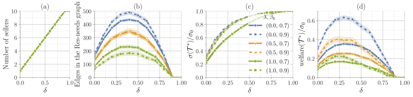
Figure 2. Panels (a) and (b) show structural properties of the resources–needs graph for the synthetic datasets with respect to increasing water availability. In Panels (c) and (d), Y-axis gives the total value $\sigma(\mathcal{T}^{*})$ and $\operatorname{welfare}(\mathcal{T}^{*})$ corresponding to an optimal assignment $\mathcal{T}^{*}$ respectively, normalized by $\sigma_{0}$, the total value when 100% of water is available. All results are for $N=10$ and the number of units per agent $k=5$. The results are shown for different values of $\lambda$ and $\beta_{h}$.

6.1. Datasets

Synthetic datasets. We consider a simple setup where there are $N$ agents $A=\{a_{i}\mid 1\leq i\leq N\}$ where a buyer can buy from any seller as long as there is value compatibility. From a domain perspective, this setup models the situation where there is a single stream, and, therefore, an agent can potentially access any other agent’s water. We will assume that all capacities and requirements are the same; that is, for all agents $a\in S\cup B$, $\gamma_{a}=k$. Water availability $\delta$ determines the fraction of water that is available. If $\delta=1$ (similarly, $\delta=0$), then all (none of the) $Nk$ units of water are available, and therefore, there is no trade. Every agent $a_{i}$ is associated with $k$ units of water. Given $\delta$, agent $a_{i}$ is a seller if and only if $\frac{i}{N}\geq 1-\delta$ (larger the $i$, the higher the priority). Agents are categorized into two types: high-valued and low-valued. For a seller $s$, we will consider a simple linear value function: $f_{s}(\ell)=\beta\ell$ for $\ell=1,\ldots,k$; high-valued agents have a larger $\beta$ than low-valued agents. Similarly, for a buyer $b$, we will consider the following linear function: $f_{b}(\ell)=\beta(k-\ell+1)$ for $\ell=1,\ldots,k$. To decide whether agent $a_{i}$ is high-valued or low-valued, we will define a probability function as follows: $p_{h}(a_{i})=\lambda\frac{i}{N}+(1-\lambda)\big{(}1-\frac{i}{N}\big{)}$, where $\lambda\in[0,1]$ is a tunable parameter. The higher the $\lambda$, the greater the probability that high priority agents are high-valued. If $\lambda=0.5$, then all agents have the same probability of $0.5$ to be assigned to the high-valued category. In our experiments, the $\beta$ value for the high-valued agent, denoted by $\beta_{h}$, is a real value between $0.5$ and $1$, and for  $\beta_{\ell}$, the $\beta$ for the low-valued agent, is set to $1-\beta_{h}$.

Real-world datasets. We used datasets containing 93 usable water rights held in the Touchet River Watershed and 77 usable water rights held in the Yakima River Watershed in the state of Washington, along with their associated farm attributes, including acreage, crop types, and volume of water needed. The value of a water unit was calculated based on value of production per acre for the relevant crop types Koong and Anderson (2022) ($n_{i}$) and the volume of water required for each field ($v_{i}$). Then, we calculated the value per acre-foot $p_{i}$ = $A_{i}\cdot n_{i}$/$v_{i}$, where $A_{i}$ is acreage, $n_{i}$ is the value of production per acre based on crop type. Buyers and sellers were decided based on water availability and water right seniority. The aggregated volumes per field $v_{i}$ were disaggregated into prioritized units of water (with unit sizes being $5$, $10$, or $20$ acre-feet). For buyers, units were prioritized in descending order of their value, while, for the sellers, units were prioritized in ascending order of their value, thus satisfying the monotonicity constraints of Algorithm 1. We created the resources–needs bipartite graph using the value functions and geographic locations of the water rights. This is described in more detail in the supplement.

6.2. Results

Figure 3. Panels (a) and (b) show structural properties of the resources–needs graph for real-world datasets with respect to increasing water availability. In Panels (c) and (d), Y-axis gives the total value $\sigma(\mathcal{T}^{*})$ and $\operatorname{welfare}(\mathcal{T}^{*})$ corresponding to an optimal assignment $\mathcal{T}^{*}$ respectively, normalized by $\sigma_{0}$, the total value when 100% of water is available. All results are for varying sizes for water units.

Compatibility graph structure and water availability. Here, we examine the structure of the buyer–seller and resources–needs compatibility graphs with increasing water availability $\delta$. For the synthetic graphs, Figure 2(a) shows a linear increase in the number of sellers, which is due to the fact that each agent is assigned the same number of resources. Note that the buyer–seller compatibility graph in this case only differs with respect to $\delta$, as all other parameters only determine the value of the water units. However, the resources–needs bipartite graph (defined in Section 4.2) is influenced significantly by combinations of seniority and value. In Plot 2(b), we observe that the number of edges in the resources–needs graph significantly decreases as the number of senior high-value agents ($\lambda$ and $\beta_{h}$ being both high) increases due to the fact that most high-value agents have water, while low-value agents who do not have water cannot buy from the former group. The corresponding set of plots for real-world datasets are in Figure 3. We note that, in this case, the number of sellers in Plot 3(a) does not increase linearly with $\delta$, particularly in the case of the Touchet networks. The curve plateaus at around $\delta=0.2$ before rising at $\delta>0.5$ in Plot 3(a). The reason for this is the existence of senior agents requiring very large numbers of water units. Until sufficient water is available, these agents will be classified as buyers instead of sellers, causing the aforementioned plateaus. Therefore, as $\delta$ is increased, the number of available water rights for trade increases abruptly. This also leads to the plateauing in Plot 3(b). Overall, we observe that heterogeneity (both quantity and crop value) in crop portfolios, seniority, and geographic constraints can lead to fewer compatible seller-buyer unit pairs. Also, the number of such pairs is relatively low in the case of Yakima.

Welfare from trade and water availability. Figures 2(c) and (d) show the benefit of trading for synthetic datasets. The total value due to trading is significantly higher when water availability is around 50%. We observe that the combination of seniority and crop value (high or low) has a significant effect. A scenario corresponding to high-value buyers and low-value sellers ($\lambda=0$) offers more opportunities for matching than the other way round ($\lambda=1$). The welfare peaks when $\delta$ is in the interval $[0.25,0.35]$, which is also the interval with the highest number of edges in the bipartite graph. The parameter $\beta_{h}$ contributes significantly to the value of welfare. The larger the $\beta_{h}$, the greater the total welfare $\sigma(\mathcal{T})$.

However, in the case of real-world datasets, we see a much richer behavior, which is partly explained by the structure of the resources–needs network. The Yakima dataset exhibits characteristics similar to those of synthetic datasets around $\delta=0.5$, but the normalized total value drops close to zero even when around 25% of the water is available (see Figure 3(c)). This is due to the same reason as that for the Touchet dataset: an agent with a large number of water units. Only for a sufficiently large value of $\delta$ does this agent get to exercise its water unit and become a seller. For the Touchet data, we observe the same phenomenon as was observed for the number of edges at $0.25\leq\delta\leq 0.5$. We note that the welfare in the case of the Touchet networks is much larger than that for Yakima, where seller-buyer compatibility is relatively low.

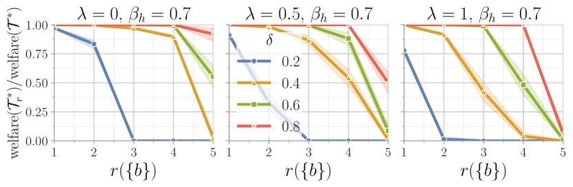
Figure 4. The loss in welfare as the lower bound on the number of water units for each individual buyer is increased. The welfare-fairness tradeoff is the ratio $\operatorname{welfare}(\mathcal{T}_{r}^{*})$/$\operatorname{welfare}(\mathcal{T}^{*})$, where $\mathcal{T}_{r}^{*}$ is an optimal solution which satisfies the fairness criteria that every buyer is matched with at least $r(\{b\})=r$ water units and $\mathcal{T}^{*}$ is an optimal solution when no such constraints are imposed. The results are for the synthetic graphs for different values of $\lambda$ and $\delta$ over 100 replicates.

Buyer satisfaction. For the synthetic networks, we find welfare maximizing solutions with the constraint that every buyer $b$ is matched to at least $r(\{b\})=r$ water units. Figure 4 shows the decrease in welfare as $r$ increases. A value of zero on the y-axis corresponds to an infeasible instance given the minimum satisfaction constraints. We note that for lower $\delta$, the maximum welfare achievable is small for even small $r$, indicating that, during water scarcity, the welfare–fairness trade off is high. For a high $\lambda$, where most buyers are low-valued and most sellers are high-valued, we see a sharp drop in welfare with increasing $r$.

For the real-world graphs, we have plotted buyer satisfaction in Figure 5 for water unit size of 10, when there are no lower bound constraints. We observe that, for both datasets, the general satisfaction levels are low for $\delta<0.5$. We see some outliers with 100% satisfaction. Upon inspection, we found that these buyers typically have a single unit requirement. We note that for Touchet10, the average buyer satisfaction jumps to $\approx 0.5$ at $\delta=0.6$. There are low-valued agents with water available at $\delta\geq 0.5$ who can lead to an increase in trade. We observe that welfare is not indicative of buyer satisfaction, as it only depends on the total value and total quantity of trade. We observe that, in general, it is challenging to guarantee a minimum number of water units to most buyers due to the fact that, in many scenarios, there are no compatible sellers for most buyers. Therefore, with the additional constraints of lower bounds as in Section 5.1, this will mostly lead to infeasible instances. Next, we note that the mean or median buyer satisfaction need not increase as $\delta$ increases. As $\delta$ increases, the number of buyers decreases. Hence, it is possible that for the remaining buyers, the buyer satisfaction is low. This explains the decrease in buyer satisfaction for Yakima10 from $\delta=0.3$ to $\delta=0.4$.

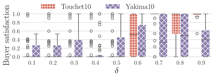
Figure 5. A boxplot of buyer satisfaction (water units matched/required water units) distribution with respect to water availability. Given the optimal solution from Algorithm 1, for each buyer, the satisfaction is computed. In some cases, the boxes are not visible. These correspond to a median of either zero or one.

The size of water units. We recall that all our proposed algorithms run in polynomial time in the number of water units. This is unlike the problems considered in Liu et al. Liu et al. (2016), where the complexity was with respect to the number of agents. Given the heterogeneity in the valuation of each water unit, this is unavoidable. One way to mitigate this problem is to increase the size of a single water unit. Our analysis on the size of water units is in the supplement.

7. Future Work

We presented results for a class of resource matching problems motivated by applications to water trading. One direction for future work is to consider optimal allocation problems with other welfare functions and fairness criteria. Our work assumes that the valuations of resources are public. If the valuations are not fully revealed (a more practical setting), interesting and richer problems involving negotiations and price discovery emerge. Our work is a step towards modeling and understanding these issues.

8. Acknowledgments

We thank the reviewers and editors for their valuable suggestions. This material is based upon work supported by the AI Research Institutes program supported by USDA-NIFA and NSF under the AI Institute: Agricultural AI for Transforming Workforce and Decision Support (AgAID) award No. 2021-67021-35344, USDA-NIFA under the Network Models of Food Systems and their Application to Invasive Species Spread, grant no. 2019-67021-29933, USDA National Institute of Food and Agriculture project #1016467, and NSF award No. OAC-1916805 (CINES). Opinions, findings, and conclusions are those of the authors and do not necessarily reflect the view of the funding entities.

Technical Supplement

Paper title:  Value-based Resource Matching with Fairness Criteria: Application to Agricultural Water Trading

Appendix A Additional Material for Section 1

A.1. Definitions of Some Combinatorial Problems

This subsection provides formal definitions of some problems which are used in various sections of the paper. These definitions can be found in several standard texts (e.g., Garey and Johnson (1979)).

(a) Exact Cover by 3-Sets (X3C)

Instance: A universal set $U=\{u_{1},u_{2},\ldots,u_{t}\}$, where $t=3\ell$ for some integer $\ell$; a collection $C=\{C_{1},C_{2},\ldots,C_{r}\}$, where each $C_{j}$ is a subset of $U$ and $|C_{j}|=3$, $1\leq j\leq r$.

Question:  Is there a subcollection $C^{\prime}$ of $C$ such that (i) the sets in $C^{\prime}$ are pairwise disjoint and (ii) the union of all the sets in $C^{\prime}$ is equal to $U$?

It is well known that X3C is NP-complete Garey and Johnson (1979). Note that when there is a solution to an X3C instance, the collection $C^{\prime}$ must have exactly $\ell=t/3$ sets since each set in $C^{\prime}$ has three elements and the sets must be pairwise disjoint.

(b) Maximum Weighted Matching in a Bipartite Graph

We recall that a matching $M$ in a graph $G(V,E)$ is a subset of edges such that no two edges of $M$ are incident on the same node West (2003). When there are weights on edges, the weight of a matching $M$ is the sum of the weights of the edges in $M$. A formal definition of the maximum weighted matching problem for bipartite graphs is as follows.

Instance: A bipartite graph $G(S,B,E)$, a weight $w(e)$ for each edge $e\in E$.

Requirement: A matching $M$ that has the maximum weight over all the matchings in $G$.

It is well known that a maximum weighted matching in a bipartite graph $G(S,B,E)$ can be computed in time $O((|S|+|B|)^{3})$ (see Table II of duan2014linear for a summary of the available algorithms and their running times).

(c) Degree Constrained Subgraph or $b$-Matching (DCS)

Instance: A bipartite graph $G(X,Y,E)$, nonnegative integers $\lambda(v)$ and $\mu(v)$ for each node $v\in X\cup Y$ such that $\lambda(v)\leq\mu(v)$.

Requirement: Is there a subgraph $G^{\prime}(X,Y,E^{\prime})$ of $G$ such that for each $v\in X\cup Y$, the degree $d(G^{\prime},v)$ of $v$ in $G^{\prime}$ satisfies the condition $\lambda(v)\leq d(G^{\prime},v)\leq\mu(v)$?

It is known that the DCS problem can be solved efficiently using a reduction to the matching problem on bipartite graphs Gabow (1983). When a solution exists, a corresponding subgraph can also be obtained efficiently.

(d) Minimum Vertex Cover (MinVC)

Instance: An undirected graph $G(V,E)$ and a positive integer $k\leq|V|$.

Question:  Is there a vertex cover $V^{\prime}\subseteq V$ of size at most $k$ for $G$ (i.e., a subset $V^{\prime}$ of nodes such that $|V^{\prime}|\leq k$ and for each edge $\{x,y\}\in E$, at least one of $x$ and $y$ is in $|V^{\prime}|$)?

It is well known that MinVC is NP-complete Garey and Johnson (1979).

Appendix B Additional Material for Section 4

B.1. Running time of Algorithm 1

The running time of the algorithm is dominated by the computation of a maximum weighted matching in Step 2. A maximum weighted matching of $G^{\prime}$ can be computed in $O((|S^{\prime}|+|B^{\prime}|)^{3})$ time (see Table II of  duan2014linear for the available algorithms and their running times).

B.2. Statement and Proof of Theorem 4.2

Statement of Theorem 4.2: Suppose we are given a set of sellers $S$, buyers $B$, their water units, compatibility graph $G(S,B,E)$, and value functions satisfying the following condition: $\forall s\in S$, $f_{s}$ is a monotone non-decreasing function. In this setting, MaxWelfare is NP-hard.

Proof: We use a decision version of MaxWelfare where the input includes an additional integer parameter $\lambda$ and the goal is to determine whether there is an assignment for which the welfare function has a value of at least $\lambda$. Our proof of NP-hardness is through a reduction from the Exact Cover by 3-Sets (X3C) problem (defined in Section A.1).

Given an instance $I$ of X3C consisting of a universal set $U=\{u_{1},u_{2},\ldots,u_{t}\}$, where $t=3\ell$, and a collection $C=\{C_{1},C_{2},\ldots,C_{r}\}$ of 3-element subsets of $U$, we construct an instance $I^{\prime}$ of MaxWelfare as follows.

1. The set $S=\{s_{1},s_{2},\ldots s_{t}\}$ of sellers is in one-to-one correspondence with the set $U$. Each seller $s_{i}$ has only one associated water unit $w^{i}$, $1\leq i\leq t$. (Thus, the set of water units on the seller side is in one-to-one correspondence with the set of sellers.)

2. The set $B=\{b_{1},b_{2},\ldots b_{r}\}$ of buyers is in one-to-one correspondence with the set collection $C$.

3. We assume that the elements of $U$ are ordered as $\{u_{1},u_{2},\ldots,u_{t}\}$ and that the elements in each subset $C_{j}\in C$ are listed in the order in which they appear in $U$. For each set $C_{j}=\{u_{j_{1}},u_{j_{2}},u_{j_{3}}\}$ of the X3C instance $I$, we create three water units $w^{j}_{1}$, $w^{j}_{2}$ and $w^{j}_{3}$ for buyer $b_{j}$, $1\leq j\leq r$. Water unit $w^{j}_{p}$ is compatible with water unit $w^{j_{p}}$ (of seller $s_{j_{p}})$, $1\leq p\leq 3$. (For example, suppose $C_{j}=\{u_{3},u_{4},u_{7}\}$. We have three water units for buyer $b_{j}$, namely $w^{j}_{1}$, $w^{j}_{2}$ an $w^{j}_{3}$; further, $w^{j}_{1}$, $w^{j}_{2}$ an $w^{j}_{3}$ are compatible with the seller water units $w^{3}$, $w^{4}$ and $w^{7}$ respectively.)

4. For each seller $s_{i}$, the value function $f_{s_{i}}$ is defined as follows: $f_{s_{i}}(w^{i})=1$, $1\leq i\leq t$. (Thus, the function $f_{s}$ associated with each seller $s$ is trivially monotone and non-decreasing.)

5. For each buyer $b_{j}$, the value function $f_{b_{j}}$ is defined as follows: $f_{b_{j}}(w^{j}_{1})=0$, $f_{b_{j}}(w^{j}_{2})=0$, and $f_{b_{j}}(w^{j}_{3})=Q$, where $Q$ is an integer $\geq 4$, $1\leq j\leq r$. (The function $f_{b}$ associated with each buyer $b$ is monotone but non-decreasing; that is, it fails to satisfy the condition needed for Theorem 4.1.)

6. The lower bound $\lambda$ on the value of the welfare function is set to $\ell(Q-3)$.

This completes the construction of the MaxWelfare instance $I^{\prime}$. Clearly, the construction can be done in polynomial time. We now show that there is a solution to the MaxWelfare instance $I^{\prime}$ iff there is a solution to the X3C instance $I$.

Suppose there is a solution $C^{\prime}$ to the X3C instance $I$. Recall that such a solution must have exactly $\ell$ sets. Without loss of generality, let the solution be given by $C^{\prime}=\{C_{1},C_{2},\ldots,C_{\ell}\}$. If $C_{j}$ = $\{u_{j_{1}},u_{j_{2}},u_{j_{3}}\}$, assign the water units $w^{j_{1}}$, $w^{j_{2}}$ and $w^{j_{3}}$ of sellers $s_{j_{1}}$, $s_{j_{2}}$ and $s_{j_{3}}$ respectively to the three units $w^{j}_{1}$, $w^{j}_{2}$ and $w^{j}_{3}$ of buyer $b_{j}$, $1\leq j\leq\ell$. (The other $r-\ell$ buyers are not assigned any water units.) Since $C^{\prime}$ covers all the elements of $U$, this assigns all the $t=3\ell$ water units of the sellers. Since the sets in $C^{\prime}$ are pairwise disjoint, each water unit of a seller is assigned to exactly one buyer. Thus, for each seller $s_{i}$, the value $f_{s_{i}}(w^{i})=1$ ($1\leq i\leq t=3\ell$), and for each buyer $b_{j}$, the value $f_{b_{j}}(w^{j}_{3})=Q$. Hence, the value of the welfare function is $\sum_{j=1}^{\ell}f_{b_{j}}(w^{J}_{3})-\sum_{i=1}^{3\ell}f_{s_{i}}(w^{i})$ = $Q\ell-3\ell$ = $\ell(Q-3)$ = $\lambda$. Thus, we have a solution to the MaxWelfare instance $I^{\prime}$.

Now suppose there is a solution to the MaxWelfare instance $I^{\prime}$. We have the following claim.

Claim 1: Any valid solution to the MaxWelfare instance $I^{\prime}$ must include the following two properties: (a) exactly $\ell$ buyers have a value of $Q$ for their value functions; and (b) all the $t=3\ell$ sellers have the value 1 for their value functions.

Proof of Claim 1: First, consider Part (a). Since the total number of available water units from the sellers is $t=3\ell$ and each buyer needs 3 units for their value-functions to have a value $Q$, at most $\ell$ buyers can have the value $Q$ for their value functions. Now, suppose for the sake of contradiction, the number $z$ of buyers with the value $Q$ for their value-functions is less than $\ell$. Such an assignment would use at least $3z$ water units of sellers (since each buyer with value function $Q$ needs three water units). Then the value of the welfare function is at most $zQ-3z$ = $z(Q-3)$. Since $z<\ell$, the value of the welfare function is $<\lambda=\ell(Q-3)$. This contradicts the assumption that the value of the welfare function is at least $\ell(Q-3)$, and completes our proof of Part (a).

To prove Part (b), note that from Part (a), the number of buyers with the value $Q$ for their value function is $\ell$. Since each such buyer is assigned three water units, it follows that the total number of water units assigned to all the buyers is $3\ell$. This completes the proof of Claim 1.  $\Box$

In view of Claim 1, any solution to instance $I^{\prime}$ has exactly $\ell$ buyers, each of whom has been assigned three water units. Without loss of generality, let $\{b_{1},b_{2},\ldots,b_{\ell}\}$ denote this set of buyers. Construct the following collection $C^{\prime}$ of subsets: for each buyer $b_{j}$ in the solution, choose the corresponding set $C_{j}$ in $C^{\prime}$, $1\leq j\leq\ell$. Since the sets of water units assigned to the buyers are pairwise disjoint and the $3\ell$ water units of the sellers are used in the solution to $I^{\prime}$, it can be seen that $C^{\prime}$ is a solution to the X3C instance $I^{\prime}$, and this completes our proof of Theorem 4.2.  

Appendix C Additional Material for Section 5

C.1. Additional Material for Section 5.1

In Section 5.1, we considered the welfare maximization problem when there are lower bounds on the number of water units to be assigned to subsets of buyers. Here, we show that, in general, the problem of determining whether there is a solution that satisfies all such lower bound constraints is itself NP-complete. It should be noted that this decision problem does not involve welfare maximization. A formal statement of the problem is as follows.

Feasibility of Demographic Constraints (FeasDemog)

Instance:  A set $S$ of sellers and their water units, a set $B$ of buyers, a resource–needs compatibility graph $G^{\prime}$, a collection $D$ of constraints of the form $(A,q)$ where $A\subseteq B$ is a subset of buyers and $q$ is a positive integer that gives a lower bound on the total number of water units to be assigned to the buyers in $A$.

Question:  Is there a valid assignment that satisfies all the constraints in $D$?

The following result establishes the complexity of the FeasDemog problem.

Proposition C.1.

The FeasDemog problem is NP-complete.

Proof: It can be seen that the FeasDemog problem is in NP since given an assignment, it is easy to efficiently check whether it satisfies all the constraints in $D$. To prove NP-hardness, we use a reduction from the MinVC problem (defined in Section A.1).

Given an instance $I$ of the MinVC problem consisting of a graph $G(V,E)$ and an integer $k\leq|V|$, we construct an instance $I^{\prime}$ of the FeasDemog problem as follows.

1. The set $S=\{s_{1},s_{2},\ldots,s_{k}\}$ consists of $k$ sellers; each seller $s_{i}$ has exactly one water unit $w_{i}$, $1\leq i\leq k$.

2. Let $|V|=\{v_{1},v_{2},\ldots,v_{n}\}$. The set $B=\{b_{1},b_{2},\ldots,b_{n}\}$ of buyers is in one-to-one correspondence with the node set $V$.

3. The resource–needs graph $G^{\prime}$ is a complete bipartite graph between the water units of sellers and the buyers. (In other words, any water unit of the sellers can be assigned to any buyer.)

4. The set $D$ has $m=|E|$ constraints. For each edge $e=\{v_{i},v_{j}\}$ of $G$, we create a constraint $(\{b_{i},b_{j}\},1)$; that is, the buyers corresponding to the end points of edge $e$ must be assigned a total of at least one water unit.

This completes the construction. It is easy to verify that the construction can be carried out in polynomial time.

Suppose there is a solution to the MinVC problem. Without loss of generality, let $V^{\prime}=\{v_{1},v_{2},\ldots,v_{k}\}$ denote the given vertex cover of size $k$. Consider the matching assignment $\mathcal{T}$ given by $\mathcal{T}$ = $\{(w_{i},b_{i})\leavevmode\nobreak\ :\leavevmode\nobreak\ 1\leq i\leq k\}$. (Recall that buyer $b_{i}$ corresponds to node $v_{i}$ of $G$.) Since the resource–needs graph is a complete bipartite graph, this assignment satisfies the compatibility conditions. To show that this assignment satisfies all the constraints in $D$, consider any constraint $(\{b_{x},b_{y}\},1)$ in $D$. This constraint was added to $D$ due to the edge $\{v_{x},v_{y}\}$ in $G$. Since $V^{\prime}$ is a vertex cover for $G$, at least one of $v_{x}$ and $v_{y}$ appears in $V^{\prime}$. Without loss of generality, let $v_{x}$ be in $V^{\prime}$. Thus, the assignment $\mathcal{T}$ gives a water unit to buyer $b_{x}$, thus satisfying the constraint $(\{b_{x},b_{y}\},1)$. Thus, we have a valid solution to the FeasDemog instance $I^{\prime}$.

Now, suppose there is a solution $\mathcal{T}$ to the FeasDemog instance $I^{\prime}$. Without loss of generality, let this solution assign water units to buyers $\{b_{1},b_{2},\ldots,b_{r}\}$ for some $r\leq k$. (Since there are only $k$ water units in total, the number $r$ of buyers to whom water units can be assigned is at most $k$.) Let $V^{\prime}=\{v_{1},v_{2},\ldots,v_{r}\}$ be the nodes corresponding to the buyers to whom water units are assigned by $\mathcal{T}$. We now show that $V^{\prime}$ is a vertex cover for $G$. Consider any edge $e=\{v_{x},v_{y}\}$ of $G$. Note that $D$ has the constraint $(\{b_{x},b_{y}\},1)$ corresponding to $e$. Since this constraint is satisfied by $\mathcal{T}$, at least one of $b_{x}$ and $b_{y}$ must be assigned a water unit. Thus, at least one of these two nodes appears in $V^{\prime}$. Thus, $V^{\prime}$ is a vertex cover of size $\leq k$ for $G$. This completes our proof of Proposition C.1.  

C.2. Additional Material for Section 5.2

The purpose of this section is to show that the MaxLeximin problem can be solved efficiently. For the reader’s convenience, we repeat the definition of the problem.

Definition of MaxLeximin problem: Given a seller with a set $W$ of $k$ water units, a set of buyers $B$ with the same cost for every water unit, and a compatibility graph $G_{w}(W,B,E_{w})$, find a trading assignment $\mathcal{T}^{*}$ with the leximin-largest buyer satisfaction vector.

As mentioned in Section 5.2, we obtain an efficient algorithm for the MaxLeximin problem by reducing it to a problem called MaxTB-MRM from Trabelsi et al. Trabelsi et al. (2023). A definition of the MaxTB-MRM problem is as follows.

Instance: A bipartite graph $G(X,Y,E^{\prime})$, where $X$ is a set of agents and $Y$ is a set of resources, a number of matching rounds, $k$. For each agent $x_{j}$, permissible set of rounds $K_{j}\subseteq[k]$, the desired number of rounds $\rho_{j}$, and a valid benefit function $\mu^{\prime}_{j}(\cdot)$.

Required: Find a collection $\mathcal{M}^{*}$ consisting of at most $k$ matchings of $G$ that maximizes the sum $\sum_{x_{j}\in X}\mu^{\prime}_{j}(\cdot)$.

The efficient algorithm for MaxTB-MRM presented in Trabelsi et al. (2023) requires that the benefit functions for agents be valid. The definition of a valid benefit function is as follows.

Valid benefit function:  For each agent $x_{j}$, let $\mu_{j}(\ell)$ denote the non-negative benefit that the agent $x_{j}$ receives if it appears in $\ell$ matchings, for $\ell=0,1,2,\ldots,\rho_{j}$. Let $\delta_{j}(\ell)=\mu_{j}(\ell)-\mu_{j}(\ell-1)$ for $\ell=1,2,\ldots,\rho_{j}$. We say that the benefit function $\mu_{j}$ is valid if it satisfies all of the following four properties: (P1) $\mu_{j}(0)=0$; (P2) $\mu_{j}$ is monotone non-decreasing in $\ell$; (P3) $\mu_{j}$ has the diminishing returns property, that is, $\mu_{j}(\ell)-\mu_{i}(\ell-1)\leq\mu_{j}(\ell-1)-\mu_{i}(\ell-2)$ for $2\leq\ell\leq\rho_{i}$; and (P4) $\delta_{j}(\ell)\leq 1$, for $\ell=1,2,\ldots,\rho_{j}$.

Note that $\mu_{j}(\cdot)$ satisfies property P3 iff $\delta_{j}(\cdot)$ is monotone non-increasing in $\ell$.

We now show that the following problem, which is related to the MaxLeximin problem, can be efficiently solved through a reduction to the MaxTB-MRM problem. (This reduction was sketched in Section 5.2.)

Finding a Trading Assignment to Maximize the Total Reward (Max-Reward-Trade)

Instance: A set $W=\{w_{1},w_{2},\ldots,w_{t}\}$ of water units, a set $B=\{b_{1},b_{2},\ldots,b_{m}\}$ of buyers, a bipartite compatibility graph $G(W,B,E)$, a requirement $\rho_{j}\leq|W|$ and a valid benefit function $\mu_{j}$ for each buyer $b_{j}$. (The benefit function $\mu_{j}(\ell)$ is defined for all $\ell$, $0\leq\ell\leq\rho_{j}$.)

Required:  Find a trading assignment $\mathcal{T}$ such that the total reward $\mathbb{B}(\mathcal{T})$ = $\sum_{j=1}^{m}\mu_{j}(\cdot)$ due to the assignment is maximized.

Lemma C.2.

The Max-Reward-Trade problem can be solved in polynomial time through a reduction to the MaxTB-MRM problem.

Proof: A reduction from the Max-Reward-Trade problem to the MaxTB-MRM problem is as follows.

1. The compatibility graph $G^{\prime}(X,Y,E^{\prime})$ is a graph with $X=B$, $Y=\{v\}$ is a single node which represents one different water right per matching round and $E^{\prime}=\{\{x,y\}|x\in X,y\in Y\}$. (Thus, $G^{\prime}$ is a star graph with a center node and $|B|$ leaves).

2. The total number of rounds is $k=|W|$ (i.e., the number of water units).

3. For each buyer $b_{j}$, $K_{j}=\{i|(v_{i},v_{j})\in E\}$ (one round per compatible water unit).

4. For each buyer $b_{j}$, the desired number of rounds is $\rho_{j}$.

5. For each buyer $b_{j}$, the benefit function is $\mu_{j}$.

Given a solution $\mathcal{M}$ to  MaxTB-MRM, we construct a trading assignment $\mathcal{T}$ as follows: each matching edge in $\mathcal{M}$ becomes one entry $(w_{i},b_{j})$ of $\mathcal{T}$; here, $w_{i}$ is determined by the matching round and $b_{j}$ by the agent. To see that an optimal solution to MaxTB-MRM provides an optimal solution to Max-Reward-Trade, consider an optimal solution $\mathcal{M}^{*}$ to MaxTB-MRM and let this correspond to a trading assignment $\mathcal{T}$ for Max-Reward-Trade. Assume for the sake of contradiction that there is a solution $\mathcal{T}^{\prime}$ such that $\mathbb{B}(\mathcal{T}^{\prime})>\mathbb{B}(\mathcal{T})$. Given $\mathcal{T}^{\prime}$, we construct a matching solution $\mathcal{M}^{\prime}$ such that for each buyer and assigned water right in $\mathcal{T}^{\prime}$, we match the corresponding buyer to the water unit in the corresponding round. It can be seen that the resulting solution is valid to MaxTB-MRM. Furthermore, its value is greater than that of $\mathbb{B}(\mathcal{M}^{*})$, contradicting the assumption that $\mathcal{M}^{*}$ is an optimal solution to the MaxTB-MRM instance. To conclude, we have an optimal solution to the Max-Reward-Trade instance. $\Box$

When the benefit function $\mu_{j}$ for each buyer $b_{j}$ has the form $\mu_{j}(\ell)=\ell$, for $0\leq\ell\leq\rho_{j}$, the total reward of all the buyers represents the total number of water units assigned. Thus, the above reduction shows that the problem of finding a trading assignment that maximizes the total number of water units assigned in the above setting can be solved efficiently.

We now address the main result which is to show that the algorithm for MaxTB-MRM in Trabelsi et al. (2023) can be used to solve the MaxLeximin problem. This is done by showing that a valid reward function for each buyer can be constructed so that maximizing the total reward produces a solution to the MaxLeximin problem. We state this result below.

Lemma C.3.

Consider any instance of the MaxLeximin problem. There exists a valid benefit function $\mu_{j}$ for each buyer $b_{j}$ such that maximizing the total benefit under this function gives a solution to the MaxLeximin problem.

We proceed to prove Lemma C.3 in several stages. We first give the procedure for constructing a valid benefit function for each buyer. The steps of this procedure are as follows. (The reader should bear in mind that $B$ and $W$ denote the set of buyers and water units, respectively, of the MaxLeximin problem. Also, for each buyer $b_{j}$, $\rho_{j}$ gives the number of water units desired by $b_{j}$.)

1. Let $F=\big{\{}k_{i}/k_{j}\mid k_{i},k_{j}\in[W]\}\leavevmode\nobreak\ \mathrm{and}\leavevmode\nobreak\ k_{i}\leq k_{j}\big{\}}\cup\{0\}$.

2. Let $\pi:F\rightarrow\{1,\ldots,|F|\}$ correspond to the index of each element in $F$ when sorted in descending order.

3. For each $q\in F$, let $\xi(q)=(|B|\cdot|W|)^{\pi(q)}/(|B|\cdot|W|)^{|F|}$. Note that each $\xi(q)\in(0,1]$.

4. The incremental benefit $\delta_{j}(\ell)$ for a buyer $b_{j}$ for the $\ell$th water unit is defined as $\delta_{j}(\ell)=\xi\big{(}(\ell-1)/\rho_{j})\big{)}$. Thus, the benefit function $\mu_{j}$ for buyer $v_{j}$ is given by $\mu_{j}(0)=0$ and $\mu_{j}(\ell)=\mu_{j}(\ell-1)+\delta_{j}(\ell)$ for $1\leq\ell\leq\rho_{j}$.

It can be seen that $\mu_{j}$ satisfies properties P1, P2 and P4 of a valid benefit function. We now show that it also satisfies P3, the diminishing returns property.

Lemma C.4.

For each buyer $b_{j}$, the incremental benefit $\delta_{j}(\ell)$ is monotone non-increasing in $\ell$. Therefore, $\mu_{j}(\cdot)$ satisfies diminishing returns property.

Proof.

By definition, for $\ell=1,\ldots,\rho_{j}-1$, $\delta_{j}(\ell)/\delta_{j}(\ell+1)=\xi\big{(}(\ell-1)/\rho_{j}\big{)}/\xi\big{(}\ell/\rho_{j}\big{)}\geq|B|\cdot|W|>1$, by noting that $\pi(\ell/\rho_{j})-\pi((\ell+1)/\rho_{j})\geq 1$. Hence, the lemma holds. ∎

To complete the proof of Lemma C.3, we must show that any solution that maximizes the benefit function defined above optimizes the leximin order. We start with some definitions and a lemma.

For a buyer $b_{j}$ and $q\in F$, let $F^{>}_{j}(q)=\{\ell\mid 0\leq\ell\leq\rho_{j}\leavevmode\nobreak\ \text{ and }\ell/\rho_{j}>q\}$. We will now show that the incremental benefit $\delta_{j}(\ell)$ obtained by buyer $b_{j}$ for matching $\ell$ is greater than the sum of all incremental benefits $\delta_{j^{\prime}}(\ell^{\prime})$, for all buyers $b_{j^{\prime}}$ and for all $\ell^{\prime}$ satisfying $\ell^{\prime}/\rho_{j^{\prime}})>\ell/\rho_{j}$.

Lemma C.5.

For any buyer $b_{j}$ and non-negative integer $\ell\leq\rho_{j}$, we have  $\delta_{j}(\ell)>\sum_{j^{\prime}\in B}\sum_{\ell^{\prime}\in F^{>}_{j^{\prime}}(\ell/\rho_{j})}\delta_{j^{\prime}}(\ell^{\prime})$.

Proof.

For any $\ell^{\prime}\in F^{>}_{j^{\prime}}(\ell/\rho_{j})$, note that $\ell/\rho_{j}<\ell^{\prime}/\rho_{j^{\prime}}$. Hence, $\pi(\ell/\rho_{j})-\pi(\ell^{\prime}/\rho_{j^{\prime}})\geq 1$. This implies that $\delta_{j}(\ell)/\delta_{j^{\prime}}(\ell^{\prime})=\xi\big{(}(\ell-1)/\rho_{j}\big{)}/\xi\big{(}(\ell^{\prime}-1)/\rho_{j^{\prime}})\big{)}\geq|W|\cdot|B|$. Since $\rho{j^{\prime}}\leq|W|$, the number of $\delta_{j^{\prime}}(\ell^{\prime})$ terms per $j^{\prime}$ is at most $|W|$. Since $\ell/\rho_{j}\notin F^{>}_{j^{\prime}}(\ell/\rho_{j})$, the number of $\delta_{j^{\prime}}(\ell)$ terms for $j^{\prime}=i$ is at most $|W|-1$. Since there are $|B|$ buyers $b_{j^{\prime}}\in B$, it follows that there are at most $|B|\cdot|W|-1$ terms $\delta_{j^{\prime}}(\ell^{\prime})$ in total. Therefore, $\sum_{j^{\prime}=i}\sum_{\ell^{\prime}\in F^{>}_{j^{\prime}}(\ell/\rho_{j}}\frac{\delta_{j^{\prime}}(\ell^{\prime})}{\delta_{j}(\ell)}<1$. ∎

We are now ready to complete the proof of Lemma C.3.

Proof of Lemma C.3. The proof is by contradiction. Suppose $\mathcal{A}^{*}$ is an optimal solution given the benefit function defined above. We will show that if there exists a solution $\mathcal{A}$ with leximin order better than that of $\mathcal{A}^{*}$, then the total benefit $\mathbb{B}(\mathcal{A})>\mathbb{B}(\mathcal{A}^{*})$, contradicting the fact that $\mathcal{A}^{*}$ is an optimal solution. Let $A=(l_{1}/\rho_{1},l_{2}/\rho_{2},...,l_{|B|}/\rho_{|B|})$ be a sorted list of satisfaction ratios for $\mathcal{A}$ and let $A^{*}=(l^{*}_{1}/\rho_{1},l^{*}_{2}/\rho_{2},...,l^{*}_{|B|}/\rho_{|B|})$ be a list defined similarly for $\mathcal{A}^{*}$. Let $k$ denote the first index for which $l_{k}/\rho_{k}\neq l^{*}_{k}/\rho_{k}$.

For a given solution $\mathcal{A}$, we use $\gamma_{j}(\mathcal{A})$ to denote the number of water rights assigned to buyer $b_{j}$, $1\leq j\leq|B|$. We recall that the benefit function for $\mathcal{A}$ can be written as $\mathbb{B}(\mathcal{A})=\sum_{j=1}^{|B|}\sum_{\ell=1}^{\gamma_{j}(\mathcal{A})}\delta_{j}(\ell)$. For each $j$, the $\delta_{j}(\ell)$ terms can be partitioned into two blocks as follows.

:

(i) $D_{1}(\mathcal{A})=\{(j,\ell)\mid\forall j,\leavevmode\nobreak\ \ell/\rho_{j}<k\}$, and

:

(ii) $D_{2}(\mathcal{A})=\{(j,\ell)\mid\forall j,\leavevmode\nobreak\ \ell/\rho_{j}\geq k$.

We can partition the terms corresponding to $\mathbb{B}(\mathcal{A}^{*})$ in the same way, and these blocks are denoted by $D_{1}(\mathcal{A}^{*})$ and $D_{2}(\mathcal{A}^{*})$. From the definition of $k$, it follows that $D_{1}(\mathcal{A}^{*})=D_{1}(\mathcal{A})$. Since $\mathcal{A}$ has a better leximin order, and, from definition, it follows that $\ell^{*}_{k}/\rho_{k}<\ell_{k}/\rho_{k}$. In addition, from the order of the ratio lists, it follows that $\ell_{k}/\rho_{k}>\ell^{*}_{j}/\rho_{j}$ for all $j>k$. From lemma C.5, it follows that $\delta_{k}(\ell_{k})>\sum_{j^{\prime}\in B}\sum_{\ell^{\prime}\in F^{>}_{j^{\prime}}(\ell/\rho_{j}}\delta_{j^{\prime}}(\ell^{\prime})$, and, therefore, $\delta_{k}(\ell_{k})>\sum_{(j,\ell)\in D_{2}(\mathcal{A}^{*})}\delta_{j}(\ell)$. Finally, we get

$$\mathbb{B}(\mathcal{A})-\mathbb{B}(\mathcal{A}^{*})= \sum_{(j,\ell)\in D_{2}(\mathcal{A})}\delta_{j}(\ell)-\sum_{(j,\ell)\in D_{2}(\mathcal{A}^{*})}\delta_{j}(\ell)$$

$$\geq\delta_{k}(\ell_{k})-\sum_{(j,\ell)\in D_{2}(\mathcal{A}^{*})}\delta_{j}(\ell)>0$$

Thus, $\mathbb{B}(\mathcal{A})>\mathbb{B}(\mathcal{A}^{*})$, and this contradicts the optimality of $\mathcal{A}^{*}$. The lemma follows. ∎

Thus, we have shown that any given instance of the MaxLeximin problem can be solved efficiently by constructing suitable benefit functions for each buyer, reducing the problem to the MaxTB-MRM problem, and then using the efficient algorithm for the MaxTB-MRM problem from Trabelsi et al. (2023). We have thus completed a proof of the following theorem (i.e., Theorem 5.3 of Section 5.2):

Theorem 5.3: An optimal solution to the MaxLeximin problem can be obtained in polynomial time.

Appendix D Additional Material for Section 6

Table 1. Datasets and their attributes.

Data	Num. agents	Total water units	Total value	Max. value	Min. value
Synthetic	10	50	variable	variable	variable
Touchet5	93	2704	8,533,475.94	57629.24	703.38
Touchet10	93	1389	8,778,037.64	115258.49	1406.77
Touchet20	93	741	9,400,712.72	230516.97	2813.54
Yakima5	77	3616	21,838,629.76	31606.52	264.33
Yakima10	77	1838	22,088,453.49	63213.04	528.66
Yakima20	77	952	22,698,607.80	126426.07	1057.31

The real-world networks were constructed using water rights data, acreage, types of crops grown, and water demand by crop type Department of Ecology, State of Washington ([n.d.]); Washington State Department of Agriculture ([n.d.]); Koong and Anderson (2022). We identified 93 water rights held in the Touchet River Watershed and 77 water rights held in the Yakima River Basin. Both of these rivers are in Washington State. The water rights were correlated with their associated farm fields, which allowed the water rights to be mapped to their corresponding crop types, acreage, and water demand. Using Washington State crop production data from the USDA National Agricultural Statistics Service (NASS) Koong and Anderson (2022), we estimated the value of production per acre for each crop type, and made educated guesses on those crop types which were not included in NASS data. We then calculated the volume of water needed per water right crop type, and assigned a monetary value to each unit of water needed. To assign the value per unit, we first calculated the total volume $v_{i}$ needed per field $i$ in acre-feet as $v_{i}$ = round($a_{i}\cdot mm_{i}/304.8$), where $a_{i}$ and $mm_{i}$ denote respectively the acreage and the volume required per acre (in acre-millimeters) of field $i$.

The total (baseline) water capacity $W$ was calculated as the sum of demands across all of the water rights per watershed (Touchet and Yakima) under normal conditions. The reduced water capacity $R$ – to account for drought conditions – was calculated as $R_{i}$ = $c_{i}$/100 * $W$ for each percentage capacity $c$ in [10% .. 90%], calculated in 10% increments. Sorting the water rights by seniority (based on priority date), more senior water rights were designated as sellers until the sum of the sellers’ water volumes would have exceeded $R$. All other, more junior, water rights were designated as buyers. Then, for each seller and buyer, we disaggregated the total volume and value per unit into separate rows by unit. For the seller, it was assumed that they would prioritize selling water for their lower value crops first, so the array of disaggregated units would be sorted by value per unit in ascending order. Similarly, buyers would probably prioritize buying water for their high-value crops first, so their array of disaggregated units was sorted by value per unit in descending order.

Finally, a bipartite graph was created, mapping each of the sellers’ units of water to compatible buyers’ units. In order to be compatible, ($i$) the buyer had to be upstream or downstream of the seller (e.g., not in different streamsheds or in different forks of the same river), and ($ii$) the buyer’s value for a given unit had to be greater than or equal to the seller’s value (or price) for that unit.

A summary of values for Yakima – based on different $R$ values – can be seen in Table 2. A few observations are worth noting. The Unit Size in Acre-Feet indicates that unit size was calculated between rows for 10 and 20 acre-feet per unit, which explains why the 20 acre-feet number of units will always be close to 50% of the 10 acre-feet number of units. Second, when dividing the acre-feet per unit size, any partial units are rounded up to the next integer value, which is why the Total Value for the 20 acre-feet unit size will always be somewhat larger than the Total Value for the corresponding 10 acre-feet unit size. There appears to be no difference between the 10% water capacity and 20% water capacity statistics because the second most senior water right included more than 20% of the total water units, which prevented the number of sellers to increase until total water capacity rose to 30%. Finally, these values are based only on the statistics for the dataset pre-experiment, or the number of units and total value that could possibly be traded, but not the actual totals from matching done during trading.

% Total Water Capacity	Unit Size in Acre-Feet	# Units	Total Value	Sellers	Buyers
10%	10	11	$27534.75	1	76
10%	20	6	$30037.91	1	76
20%	10	11	$27534.75	1	76
20%	20	6	$30037.91	1	76
30%	10	542	$10,664,614.78	8	69
30%	20	276	$10,795,007.24	8	69
40%	10	705	$14,590,442.54	26	51
40%	20	366	$14,872,635.68	26	51
50%	10	905	$14,980,581.61	37	40
50%	20	471	$15,287,062.66	37	40
60%	10	1060	$15,321,802.09	46	31
60%	20	551	$15,639,329.06	46	31
70%	10	1270	$19,918,785.39	57	20
70%	20	659	$20,363,049.477	57	20
80%	10	1435	$20,386,759.85	63	14
80%	20	745	$20,882,922.60	63	14
90%	10	1556	$20,630,547.56	68	9
90%	20	807	$21,134,945.99	68	9

Table 2. Value breakdown and seller-buyer ratios for the Yakima dataset for unit-sizes 10 and 20 acre-feet per unit.

The size of water units. We recall that all our proposed algorithms run in polynomial time in the number of water units. This is unlike the problems considered in Liu et al. Liu et al. (2016), where the complexity was with respect to the number of agents. Given the heterogeneity in the valuation of each water unit, this is unavoidable. One way to mitigate this problem is to increase the size of a single water unit. Our results in Figure 3 compare networks with different water unit resolutions with respect to both the structural properties and the welfare from trade. We note that Plot (a) is not affected by the coarsening of the resolution, i.e., the number of sellers remains the same as a function of $\delta$. However, we do see a benefit of coarsening, as it greatly reduces the number of edges in the resources–needs compatibility graphs as the size of a water unit is increased. However, we observe that coarsening has very little effect on total value. We do observe a significant difference in the welfare curves of Touchet10 and Touchet20. We note that for any fixed value of $\delta$, the greater the size of the water unit, the greater is the welfare. This is mainly due to rounding effects that lead to an increase in the total number of water units. However, the trend remains the same across different sizes.

References

- (1)
- Alon (2006) Noga Alon. 2006. Splitting digraphs. Combinatorics, Probability and Computing 15 (2006), 933–937.
- andd N. Cohen and Havet (2016) J. Bang-Jensen andd N. Cohen and F. Havet. 2016. Finding good 2-partitions of digraphs II. Enumerable properties. Theoretical Computer Science 640 (2016), 1–19.
- Basu (2023) Reetwika Basu. 2023. Three Essays on Agent-Based Models for Water Allocation under Appropriative Rights. PhD thesis. Washington State University.
- Booker and Young (1994) James F Booker and Robert A Young. 1994. Modeling intrastate and interstate markets for Colorado River water resources. Journal of Environmental Economics and Management 26, 1 (1994), 66–87.
- Brajer et al. (1989) Victor Brajer, AL Church, Ronald Cummings, and Phillip Farah. 1989. The strengths and weaknesses of water markets as they affect water scarcity and sovereignty interests in the West. Nat. Resources J. 29 (1989), 489.
- Burke et al. (2004) Susan M Burke, Richard M Adams, and Wesley W Wallender. 2004. Water banks and environmental water demands: Case of the Klamath Project. Water Resources Research 40, 9 (2004), 1–9.
- Caragiannis and Narang (2023) Ioannis Caragiannis and Shivika Narang. 2023. Repeatedly matching items to agents fairly and efficiently. In International Symposium on Algorithmic Game Theory. Springer, New York, NY, 347–364.
- Chen and Liu (2020) Xingyu Chen and Zijie Liu. 2020. The Fairness of Leximin in Allocation of Indivisible Chores. ArXiv Report: 2005.04864v1.
- Chong and Sunding (2006) Howard Chong and David Sunding. 2006. Water markets and trading. Annu. Rev. Environ. Resour. 31 (2006), 239–264.
- Cook and Rabotyagov (2014) Joseph Cook and Sergey S Rabotyagov. 2014. Assessing irrigators’ preferences for water market lease attributes with a stated preferences approach. Water Resources and Economics 7 (2014), 19–38.
- Dang et al. (2016) Qian Dang, Megan Konar, Jeffrey J Reimer, Giuliano Di Baldassarre, Xiaowen Lin, and Ruijie Zeng. 2016. A theoretical model of water and trade. Advances in Water Resources 89 (2016), 32–41.
- Deng et al. (2007) Xiaotie Deng, Li-Sha Huang, and Minming Li. 2007. On Walrasian price of CPU time. Algorithmica 48 (2007), 159–172.
- Department of Ecology, State of Washington ([n.d.]) Department of Ecology, State of Washington. [n.d.]. Water rights. https://appswr.ecology.wa.gov/waterrighttrackingsystem/WaterRights/default.aspx. [Accessed Apr-2023].
- Duan and Su (2012) Ran Duan and Hsin-Hao Su. 2012. A scaling algorithm for maximum weight matching in bipartite graphs. In Proceedings of the twenty-third annual ACM-SIAM symposium on Discrete Algorithms. SIAM, 1413–1424.
- Edmonds and Karp (1972) J. Edmonds and R. M. Karp. 1972. Theoretical improvements in algorithmic efficiency for network flow problems. J. ACM 19, 2 (1972), 248–264.
- Esmaeili et al. (2023) Seyed Esmaeili, Sharmila Duppala, Davidson Cheng, Vedant Nanda, Aravind Srinivasan, and John P Dickerson. 2023. Rawlsian fairness in online bipartite matching: Two-sided, group, and individual. In Proceedings of the AAAI Conference on Artificial Intelligence, Vol. 37. AAAI Press, Online, 5624–5632.
- Food and Organization (2022) Food and Agriculture Organization. 2022. The State of the World’s Land and Water Resources for Food and Agriculture – Systems at breaking point. Rome, Online.
- Gabow (1983) H. N. Gabow. 1983. An Efficient Reduction Technique for Degree-Constrained Subgraph and Bidirected Network Flow Problems. In Proceedings of the 15th Annual ACM Symposium on Theory of Computing, 25-27 April, 1983, Boston, Massachusetts, USA. ACM, New York, NY, 448–456.
- Gandhi et al. (2006) Rajiv Gandhi, Samir Khuller, Srinivasan Parthasarathy, and Aravind Srinivasan. 2006. Dependent rounding and its applications to approximation algorithms. J. JACM 53, 3 (2006), 324–360.
- Garey and Johnson (1979) M. R. Garey and D. S. Johnson. 1979. Computers and Intractability: A Guide to the Theory of NP-Completeness. W. H. Freeman and Co., San Francisco, CA.
- Howe (2013) Charles W Howe. 2013. Interbasin transfers of water: Economic issues and impacts. Routledge, New York, NY.
- Howe and Goemans (2003) Charles W Howe and Christopher Goemans. 2003. Water transfers and their impacts: Lessons from three Colorado water markets 1. JAWRA Journal of the American Water Resources Association 39, 5 (2003), 1055–1065.
- Kallis (2008) Giorgos Kallis. 2008. Droughts. Annual Review of Environment and Resources 33 (2008), 85–118.
- Khorasany et al. (2020) Mohsen Khorasany, Reza Razzaghi, Ali Dorri, Raja Jurdak, and Pierluigi Siano. 2020. Paving the path for two-sided energy markets: An overview of different approaches. IEEE Access 8 (2020), 223708–223722.
- Koong and Anderson (2022) Dennis Koong and Steve Anderson. 2022. 2022 WASHINGTON ANNUAL STATISTICAL BULLETIN. https://www.nass.usda.gov/Statistics_by_State/Washington/Publications/Annual_Statistical_Bulletin/2022/WA_ANN_2022.pdf. [Accessed 08-Oct-2023].
- Leonard et al. (2019) Bryan Leonard, Christopher Costello, and Gary D Libecap. 2019. Expanding water markets in the western United States: Barriers and lessons from other natural resource markets. Review of Environmental Economics and Policy 13, 1 (2019), 43–61.
- Lesmana et al. (2019) Nixie S Lesmana, Xuan Zhang, and Xiaohui Bei. 2019. Balancing efficiency and fairness in on-demand ridesourcing. Advances in neural information processing systems 32 (2019), 5310–5320.
- Li et al. (2017) Zhiyuan Li, Yicheng Liu, Pingzhong Tang, Tingting Xu, and Wei Zhan. 2017. Stability of generalized two-sided markets with transaction thresholds. In Proceedings of the 16th Conference on Autonomous Agents and MultiAgent Systems. IFAAMAS, Online, 290–298.
- Liu et al. (2016) Yicheng Liu, Pingzhong Tang, Tingting Xu, and Hang Zheng. 2016. Optimizing trading assignments in water right markets. In Proc. AAAI Conference on Artificial Intelligence, Vol. 30. AAAI Press, Online, 551–557.
- Lovász and Plummer (1986) L. Lovász and M. D. Plummer. 1986. Matching Theory. North Holland, Amsterdam, The Netherlands.
- Ma et al. (2022) Will Ma, Pan Xu, and Yifan Xu. 2022. Group-level Fairness Maximization in Online Bipartite Matching. In Proceedings of the 21st International Conference on Autonomous Agents and Multiagent Systems. IFAAMAS, Online, 1687–1689.
- Market (2023) Western Water Market. 2023. Information on Water Markets in Western USA. https://westernwatermarket.com/. [Accessed 04-10-2023].
- Moulin (2004) Herve Moulin. 2004. Fair Division and Collective Welfare. MIT Press, Cambridge, MA.
- Narang et al. (2022) S. Narang, A. Biswas, and Y. Narahari. 2022. On Achieving Fairness and Stability in Many-to-One Matchings. ArXiv Report: 2009.05823v4.
- Noori et al. (2021) Mahsa Noori, Alireza Emadi, and Ramin Fazloula. 2021. An agent-based model for water allocation optimization and comparison with the game theory approach. Water Supply 21, 7 (2021), 3584–3601.
- Panda et al. (2022) Atasi Panda, Anand Louis, and Prajakta Nibhorkar. 2022. Bipartite matchings with group fairness and individual fairness constraints. ArXiv preprint arXiv:2208.09951.
- Project (2019) Trout Unlimited Washington Water Project. 2019. Landowner’s guide to Washington water rights. https://appswr.ecology.wa.gov/docs/WaterRights/wrwebpdf/landownerguide-2019.pdf. [Accessed 08-Apr-2023].
- Raffensperger and Milke (2017) John F. Raffensperger and Mark W. Milke. 2017. Participants in and components of the smart market institution. In Smart markets for water resources: a manual for implementation. Springer, Heidelberg, Germany, 95–136.
- Raffensperger et al. (2009) John F. Raffensperger, Mark W. Milke, and E. Grant Read. 2009. A deterministic smart market model for groundwater. Operations Research 57, 6 (2009), 1333–1346.
- Sandholm and Suri (2002) Tuomas Sandholm and Subhash Suri. 2002. Optimal clearing of supply/demand curves. In International Symposium on Algorithms and Computation. Springer, New York, NY, 600–611.
- Selman et al. (2009) Mindy Selman, Evan Branosky, Cy Jones, and Jenny Guiling. 2009. Water quality trading programs: An international overview. Issue brief, World Resources Institute (WRI), Washington, DC.
- Sharghi and Kerachian (2022) Soroush Sharghi and Reza Kerachian. 2022. An uncertainty-based smart market model for groundwater management. Water Supply 22, 3 (2022), 3352–3373.
- Stiebitz (1996) Michael Stiebitz. 1996. Decomposing Graphs Under Degree Constraints. J. Graph Theory 23, 3 (1996), 321–324.
- Trabelsi (2024) Yohai Trabelsi. 2024. Code and Data: Value-based Resource Matching with Fairness Criteria: Application to Agricultural Water Trading. https://github.com/yohayt/Value_based_Resource_Matching_with_Fairness_Criteria_Application_to_Agricultural_Water_Trading.
- Trabelsi et al. (2023) Yohai Trabelsi, Abhijin Adiga, Sarit Kraus, S. S. Ravi, and Daniel J Rosenkrantz. 2023. Resource sharing through multi-round matchings. In Proceedings of the AAAI Conference on Artificial Intelligence. AAAI Press, Online, 11681–11690.
- Washington State Department of Agriculture ([n.d.]) Washington State Department of Agriculture. [n.d.]. Agricultural Land Use. https://agr.wa.gov/departments/land-and-water/natural-resources/agricultural-land-use. [Accessed Apr-2023].
- Waxman et al. (2021) Naftali Waxman, Noam Hazon, and Sarit Kraus. 2021. Manipulation of -Coalitional Games on Social Networks. ArXiv Report: 2105.09852v1.
- Waxman et al. (2020) Naftali Waxman, Sarit Kraus, and Noam Hazon. 2020. On Maximizing Egalitarian Value in -Coalitional Hedonic Games. ArXiv Report: 2001.10772v1.
- West (2003) D. B. West. 2003. Introduction to Graph Theory. Prentice-Hall, Inc., Englewood Cliffs, NJ.
- Wheeler (2021) Sarah A Wheeler (Ed.). 2021. Water Markets: A Global Assessment. Edward Elgar Publishing, Cheltenham, UK.
- Xu et al. (2018) Tingting Xu, Hang Zheng, Jianshi Zhao, Yicheng Liu, Pingzhong Tang, YC Ethan Yang, and Zhongjing Wang. 2018. A two-phase model for trade matching and price setting in double auction water markets. Water Resources Research 54, 4 (2018), 2999–3017.