Prediction of air pollutants PM₁₀ by ARBX(1) processes

Abstract

This work adopts a Banach-valued time series framework for estimation and prediction, from temporal correlated functional data, in presence of exogenous variables. The consistency of the proposed functional predictor is illustrated in the simulation study undertaken. Air pollutants PM₁₀ curve forecasting, in the Haute–Normandie region (France), is addressed, by implementation of the functional time series approach presented.

1 Introduction

In the literature, several approaches have been adopted in the analysis of pollution data (see, e.g., Pang09 , for a comparative study). In Zhangetal18 , the singular value decomposition is applied to identify spatial air pollution index (API) patterns, in relation to meteorological conditions in China. A novel hybrid model, combining Multilayer perceptron model and Principal Component Analysis (PCA), is introduced in He15 , to improve the air quality prediction accuracy in urban areas. Factor analysis and Box–Jenkins methodology are considered in Gocheva14 , to examine concentrations of primary air pollutants such as NO, NO₂ , NO_x , PM${}_{10},$ SO₂ and ground level O₃ in the town of Blagoevgrad, Bulgaria. Since PM₁₀ are inhalable atmospheric particles, their forecast has became crucial aimed at adopting efficient public transport policies. In the recent literature, one can find several modelling approaches for PM₁₀ forecasting. Among the most common statistical techniques applied, we mention multiple regression, non–linear state space modelling and artificial neural networks (see, e.g., GrivasChaloulakou06 ; Paschalidouetal11 ; Slinietal06 ; Stadloberetal08 ; Zolghadrietal06 ). Functional Data Analysis (FDA) techniques also play a crucial role in air quality forecasting (see Febreroetal08 ; Fernandezetal05 ; Ignaccoloetal14 , among others). Related meteorological variables can also be functional predicted from a functional time series framework (see, e.g., Besseetal00 ; RuizEspejo12 ; RuizMedinaetal14 ).

Computational advances have made possible the implementation of flexible models for random elements in function spaces. FDA techniques have emerged in the local analysis of high–dimensional data, which are functional in nature (see the monographs GoiaVieu16 ; HorvathKokoszka12 ; HsingEubank15 , and the references therein). Parametric functional linear time series techniques are fast and computational low-cost. In contrast with the more flexible nonparametric functional statistical approach (see, e.g.,FerratyVieu06 ), the so–called curse of dimensionality problem (see Geenens11 ; Vieu18 ) is mitigated. The semi-parametric framework also provides a partial solution to this problem (see, e.g., AneirosVieu08 ; GoiaVieu15 , in the semi–functional regression context).

From a theoretical point of view, parametric functional linear time series techniques have been widely studied in the last few decades. In particular, in the autoregressive Hilbertian process framework, the asymptotic properties of componentwise estimators of the autocorrelation operator, and their associated plug-in predictors have been derived in Bosq00 ; Mas04 ; Mas07 , among others. Recently, in Alvarezetal17 and RuizAl19 , alternative operator norms for consistency have been investigated. See also Alvarezetal16 , for the case of Ornstein–Uhlenbeck process in Hilbert and Banach spaces.

Linear parametric approaches have also been adopted in a Banach-valued time series framework. This literature has mainly been focused on the spaces of continuous functions $\mathcal{C}([0,1])$ with the supremum norn (see BuenoKlepsch18 ; DehlingSharipov05 ; LabbasMourid02 ; Parvardehetal17 , among others), and on the Skorokhod space of right–continuous functions on $[0,1],$ having limit to the left at each $t\in[0,1],$ equipped with the Skorokhod topology, usually denoted as $\mathcal{J}_{1}$–topology (see, e.g., BlankeBosq16 ; Hajj11 ). The lack of an inner product structure is supplied in RuizAlvarez18_JMVA , by considering suitable embeddings into related Hilbert spaces. In the Banach context, authors mostly focused on finding a finer scaler of norms for measuring the local regularity. Specifically, this paper proves strong consistency of a componentwise estimator of the autocorrelation operator and its associated plug–in predictor, in an abstract Banach–valued time series framework, under the opposite motivation: measuring the local singularity in an accurately way.

A first attempt for the inclusion of exogenous information in the functional time series framework can be found in DamonGuillas02 , where the so-called ARHX(1) processes (Hilbert-valued autoregressive processes of order one with exogenous variables) are introduced. Enhancements were subsequently proposed by DamonGuillas05 ; MarionPumo04 . First order conditional autoregressive Hilbertian processes were introduced in Guillas02 . The present paper extends the time series framework in RuizAlvarez18_JMVA to the case of first-order Banach-valued autoregressive processes with exogenous variables (ARBX(1) processes). Functional parameter estimation and plug–in prediction can be addressed in our ARBX(1) context, from the multivariate infinite–dimensional formulation of the results in RuizAlvarez18_JMVA . Specifically, a matrix–operator–based formulation of the ARB(1) process (Banach–valued autoregressive process of order one) state equation is considered. The required Hilbert space embeddings, and sufficient conditions for the strong–consistency of the autocorrelation operator estimator (reflecting temporal correlations between endogenous and exogenous variables), and the associated plug–in functional predictor, are then obtained in a direct way. We refer to the reader to Triebel83 , where several examples of the Banach space context introduced in RuizAlvarez18_JMVA can be found.

The outline of the paper is as follows. The ARBX(1) based estimation and prediction methodologies presented are described in Section 2. Some basic concepts about nuclear and Besov spaces are introduced in Section 3, as well as a discussion about how assumptions are verified in the scenarios adopted. A simulation study is undertaken, to illustrate the consistency of ARBX(1) predictors, in Section 4. PM₁₀ short-term forecasting, based on the introduced ARBX(1) framework, is addressed in Section 5. Final comments, and discussion about how the extension to an spatiotemporal analysis, are provided in Section 6. Some extra Figures and Tables can be found in the Appendix. The main theoretical proofs required for the development of the results, as well as more detailed definitions of Besov spaces, can be checked in the Supplementary Material provided.

2 ARBX(1) estimation and prediction

In the following, the functional random variables and stochastic processes introduced below are defined on the basic probability space $\left(\Omega,\mathcal{A},\mathcal{P}\right).$ Let $\left(B,\left\|\cdot\right\|_{B}\right)$ be a real separable Banach space with associated norm $\left\|\cdot\right\|_{B}.$ Consider $X=\left\{X_{n},\ n\in\mathbb{Z}\right\}$ to be a zero-mean ARB(1) process, with $P[X_{n}\in B]=1,$ $n\in\mathbb{Z},$ satisfying the following state equation (see, e.g., Bosq00 ):

$$X_{n}=\rho\left(X_{n-1}\right)+\varepsilon_{n},\quad n\in\mathbb{Z},$$ (1)

where $\rho$ is the autocorrelation operator, which is assumed to be a bounded linear operator on $B,$ that is, $\rho\in\mathcal{L}(B),$ with $\left(\mathcal{L}(B),\left\|\cdot\right\|_{\mathcal{L}(B)}\right)$ denoting the Banach space of continuous operators with the supremum norm. Here, $\varepsilon=\left\{\varepsilon_{n},\ n\in\mathbb{Z}\right\}$ represents the innovation process, which is assumed to be a $B$-valued strong white noise, and uncorrelated with the random initial condition. In particular, $\sigma_{\varepsilon}^{2}={\rm E}{\color[rgb]{0,0,1}\left[\left\|\varepsilon_{n}\right\|_{B}^{2}\right]}<\infty,$ $n\in\mathbb{Z}.$ From (Bosq00, , Theorem 6.1), if there exists $j_{0}\geq 1$ such that $\left\|\rho^{j}\right\|_{\mathcal{L}\left(B\right)}<1,$ for every $j\geq j_{0},$ then, equation (1) admits a unique stationary solution $X_{n}=\sum_{j=0}^{\infty}\rho^{j}\left(\varepsilon_{n-j}\right)$, with $\sigma_{X}^{2}={\rm E}{\color[rgb]{0,0,1}\left[\left\|X_{n}\right\|_{B}^{2}\right]}<\infty,$ $n\in\mathbb{Z}.$

In this paper, exogenous information is incorporated to equation (1) in an additive way. Thus, the state equation of an ARBX(1) process will be established as follows:

$$X_{n}=\rho\left(X_{n-1}\right)+\displaystyle\sum_{i=1}^{b}a_{i}\left(Z_{n,i}\right)+\varepsilon_{n},\quad n\in\mathbb{Z},$$ (2)

where $\left\{a_{i},\ i=1,\ldots,b\right\}$ are bounded linear operators on $B.$ The exogenous functional random variables $Z_{i}=\{Z_{n,i},\ n\in\mathbb{Z}\},$ $i=1,\ldots,b,$ are assumed to satisfy the following ARB(1) equation, for $i=1,\ldots,b,$

$$Z_{n,i}=u_{i}\left(Z_{n-1,i}\right)+\eta_{n,i},\quad u_{i}\in\mathcal{L}(B),\quad n\in\mathbb{Z}.$$ (3)

For $i=1,\dots,b,$ $\eta_{i}=\left\{\eta_{n,i}\ n\in\mathbb{Z}\right\}$ is a $B$-valued strong white noise. Particularly, $\sigma_{\eta_{i}}^{2}={\rm E}\left[\left\|\eta_{n,i}\right\|_{B}^{2}\right]<\infty,$ $n\in\mathbb{Z},$ $i=1,\dots,b.$ Here, $P[Z_{n,i}\in B]=1,\quad{\rm E}\left[Z_{n,i}\right]=0_{B},$ $n\in\mathbb{Z},$ for $i=1,\ldots,b.$ The symbol $0_{B}$ means the zero element (null function) in $B.$ Equations (2)–(3) can be rewritten as (see DamonGuillas02 ),

$$\overline{X}_{n} = \overline{\rho}\left(\overline{X}_{n-1}\right)+\overline{\varepsilon}_{n},\quad\overline{\rho}\in\mathcal{L}(\overline{B}),\quad P[\overline{X}_{n}\in\overline{B}]=P[\overline{\varepsilon}_{n}\in\overline{B}]=1,$$ (4)

where $\overline{B}=B^{b+1}$ is also a real separable Banach space (see Lemma 1 and Proposition 1 in the Supplementary Material provided), and

$$\overline{X}_{n}=\begin{pmatrix}X_{n}\\ Z_{n+1,1}\\ Z_{n+1,2}\\ \vdots\\ Z_{n+1,b}\end{pmatrix},\quad\overline{\varepsilon}_{n}=\begin{pmatrix}\varepsilon_{n}\\ \eta_{n,1}\\ \eta_{n,2}\\ \vdots\\ \eta_{n,b}\end{pmatrix},\quad\overline{\rho}=\begin{pmatrix}\rho&a_{1}&{\color[rgb]{0,0,1}a_{2}}&{\color[rgb]{0,0,1}a_{3}}&\cdots&{\color[rgb]{0,0,1}a_{b-1}}&a_{b}\\ \mathbf{0}_{B}&u_{1}&\mathbf{0}_{B}&{\color[rgb]{0,0,1}\mathbf{0}_{B}}&\cdots&{\color[rgb]{0,0,1}\mathbf{0}_{B}}&\mathbf{0}_{B}\\ \mathbf{0}_{B}&\mathbf{0}_{B}&u_{2}&\mathbf{0}_{B}&{\color[rgb]{0,0,1}\cdots}&{\color[rgb]{0,0,1}\mathbf{0}_{B}}&{\color[rgb]{0,0,1}\mathbf{0}_{B}}\\ \vdots&\vdots&{\color[rgb]{0,0,1}\vdots}&{\color[rgb]{0,0,1}\vdots}&\ddots&{\color[rgb]{0,0,1}\vdots}&{\color[rgb]{0,0,1}\vdots}\\ {\color[rgb]{0,0,1}\mathbf{0}_{B}}&{\color[rgb]{0,0,1}\mathbf{0}_{B}}&{\color[rgb]{0,0,1}\mathbf{0}_{B}}&{\color[rgb]{0,0,1}\mathbf{0}_{B}}&{\color[rgb]{0,0,1}\cdots}&{\color[rgb]{0,0,1}\mathbf{0}_{B}}&{\color[rgb]{0,0,1}\mathbf{0}_{B}}\\ {\color[rgb]{0,0,1}\mathbf{0}_{B}}&{\color[rgb]{0,0,1}\mathbf{0}_{B}}&{\color[rgb]{0,0,1}\mathbf{0}_{B}}&{\color[rgb]{0,0,1}\mathbf{0}_{B}}&{\color[rgb]{0,0,1}\cdots}&{\color[rgb]{0,0,1}u_{b-1}}&{\color[rgb]{0,0,1}\mathbf{0}_{B}}\\ \mathbf{0}_{B}&\mathbf{0}_{B}&{\color[rgb]{0,0,1}\mathbf{0}_{B}}&\mathbf{0}_{B}&\cdots&{\color[rgb]{0,0,1}\mathbf{0}_{B}}&u_{b}\end{pmatrix}.$$ (5)

Here, $\mathbf{0}_{B}$ represents the null operator on $B.$ In equation (4), $\mathcal{L}(\overline{B})$ denotes the space of bounded linear operators on $\overline{B},$ endowed with the norm

$$\left\|\overline{y}\right\|_{\overline{B}}=\displaystyle\sup_{n\geq 1}\left|\overline{F}_{n}(\overline{y})\right|=\sup_{n\geq 1}\sup_{i\in\{1,\dots,b+1\}}\quad\left|F_{ni}(y_{i})\right|,\quad\overline{F}_{n}=\left(F_{n1},\dots,F_{n(b+1)}\right),$$ (6)

for every $\overline{y}=(y_{1},\dots,y_{b+1})\in\overline{B}=B^{b+1}.$ Here, for $i=1,\dots,b,$ $\{F_{ni},\ n\geq 1\}\subset B^{\star}$ is a sequence of bounded linear functionals on $B$ satisfying

$$F_{ni}\left(x_{ni}\right)=\left\|x_{ni}\right\|_{B},\quad\left\|F_{ni}\right\|=1,\quad n\geq 1,$$ (7)

with $\{x_{ni},\ n\geq 1\}\subset B$ being a dense sequence in $B$ (see Lemma 2.1 in Kuelbs70 for more details). For simplification purposes, we consider a common dense system in $B,$ i.e., $x_{n}=x_{ni},$ and $F_{ni}=F_{n},$ for $i=1,\dots,b,$ and $n\geq 1.$ We will assume the conditions ensuring the existence of a unique stationary solution to equation (4). That is, assume that there exists a $j_{0}$ such that $\|\overline{\rho}^{j}\|_{\mathcal{L}(\overline{B})}<1,$ for all $j\geq j_{0}.$ The following componentwise estimator of the autocorrelation operator $\overline{\rho}$ in (4), based on a functional sample of size $n,$ is then formulated:

$$\widetilde{\overline{\rho}}_{k_{n}}(\overline{x})=\left(\widetilde{\Pi}^{k_{n}}\overline{D}_{n}\overline{C}_{n}^{-1}\widetilde{\Pi}^{k_{n}}\right)(\overline{x})=\left(\displaystyle\sum_{j=1}^{k_{n}}\frac{1}{C_{n,j}}\langle\overline{x},\overline{\phi}_{n,j}\rangle_{\widetilde{\overline{H}}}\widetilde{\Pi}^{k_{n}}\overline{D}_{n}(\overline{\phi}_{n,j})\right),$$ (8)

where, for $j\geq 1,$

$$\langle\overline{x},\overline{\phi}_{n,j}\rangle_{\widetilde{\overline{H}}}=\left\langle x,\phi_{n,j1}\right\rangle_{\widetilde{H}}+\sum_{i=1}^{b}\left\langle x_{i},\phi_{n,j(i+1)}\right\rangle_{\widetilde{H}},\quad\forall\overline{x}=(x,x_{1},\cdots,x_{b})\in\overline{B},$$

with $\{\overline{\phi}_{n,j}=(\phi_{n,j1},\cdots,\phi_{n,j(b+1)}),\ j\geq 1\}$ being the orthonormal eigenfunctions system associated with

$$\overline{C}_{n}=\frac{1}{n}\sum_{i=1}^{n}\overline{X}_{i}\otimes\overline{X}_{i},$$

the empirical autocovariance operator of the extended version to $\widetilde{\overline{H}}=\widetilde{H}^{b+1},$ of $\overline{X}=\{\overline{X}_{n},\ n\in\mathbb{Z}\}.$ Here, the Hilbert space $\widetilde{H}$ is defined in Lemma 2.1 in Kuelbs70 , as the continuous extension of the separable real–valued Banach space $B$ (see also Lemma 1 in RuizAlvarez18_JMVA ). In particular, its inner product is given by $\left\langle f,g\right\rangle_{\widetilde{H}}=\sum_{n=1}^{\infty}t_{n}F_{n}(f)F_{n}(g),$ for $f,g\in\widetilde{H},$ with $\sum_{n=1}^{\infty}t_{n}=1,$ $t_{n}>0,$ $n\geq 1.$ Note that $\widetilde{H}$ has weaker topology than $B,$ allowing the continuous inclusion $B\hookrightarrow\widetilde{H},$ and hence, $\overline{B}\hookrightarrow\widetilde{\overline{H}},$ holds. In (8), for each functional sample of size $n,$ we have denoted

$$\widetilde{\Pi}^{k_{n}}\left(\overline{x}\right) = \displaystyle\sum_{j=1}^{k_{n}}\langle\overline{x},\overline{\phi}_{n,j}\rangle_{\widetilde{\overline{H}}}\overline{\phi}_{n,j},\quad\forall\overline{x}\in\overline{B}=B^{b+1}\subset\widetilde{\overline{H}}=\widetilde{H}^{b+1}.$$ (9)

Denote also by $\{C_{n,j},\ j\geq 1\},$ with $C_{n,1}\geq\dots\geq C_{n,n}\geq 0=C_{n,n+1}=C_{n,n+2}=\dots,$ the eigenvalues of $\overline{C}_{n}$ respective associated with the empirical eigenfunctions $\{\overline{\phi}_{n,j},\ j\geq 1\}.$ The operator $\overline{D}_{n}=\frac{1}{n-1}\sum_{i=1}^{n-1}\overline{X}_{i}\otimes\overline{X}_{i+1}$ denotes the empirical cross–covariance operator of the extended version of $\overline{X}_{n}$ to $\widetilde{\overline{H}}.$

In RuizAlvarez18_JMVA , sufficient conditions are derived to ensure the strong consistency in the space $\mathcal{L}(\overline{B})$ (i.e., with respect to the supremum norm in $\mathcal{L}(\overline{B})$) of the componentwise functional parameter estimator (8) of $\overline{\rho},$ formulated in the weaker topology of $\widetilde{\overline{H}},$ where countable orthogonal systems, like $\{\overline{\phi}_{n,j},\ j\geq 1\},$ can be considered from its separability. Specifically, the following conditions are assumed in RuizAlvarez18_JMVA :

• Assumption A1. $\|\overline{X}_{0}\|_{\overline{B}}$ is almost surely bounded. The eigenspaces associated with the eigenvalues of $\overline{C}=E\left[\overline{X}_{n}\otimes\overline{X}_{n}\right]$ are one–dimensional.

• Assumption A2. Let $k_{n}$ be such that $C_{n,k_{n}}>0$ a.s., and both $k_{n}\to\infty$ and ${k_{n}}/{n}\to 0$ as $n\to\infty$. Here, $C_{n,k_{n}}$ denotes the $k_{n}$–th eigenvalue of $\overline{C}_{n}.$

• Assumption A3. As $k\to\infty$,

  $$\sup_{\overline{x}\in\overline{B},\ \|\overline{x}\|_{\overline{B}}\leq 1}\left\|\overline{\rho}(\overline{x})-\sum_{j=1}^{k}\langle\overline{\rho}(\overline{x}),\overline{\phi}_{j}\rangle_{\widetilde{\overline{H}}}\overline{\phi}_{j}\right\|_{\overline{B}}\to 0,\quad\overline{\phi}_{j}=(\phi_{j1},\dots,\phi_{j(b+1)}),\ j\geq 1,$$

  where $\overline{C}(\overline{\phi}_{j})=C_{j}\overline{\phi}_{j},$ $j\geq 1,$ in $\widetilde{\overline{H}}.$

• Assumption A4. Denote by $\mathcal{H}(\overline{X})$ the reproducing kernel Hilbert space generated by $\overline{C}.$ The inclusion of $\mathcal{H}(\overline{X})$ into $\widetilde{\overline{H}}^{\star}$ is continuous, i.e., $\mathcal{H}(\overline{X})\hookrightarrow\widetilde{\overline{H}}^{\star},$ is a continuous mapping, where $\widetilde{\overline{H}}^{\star}$ denotes the dual Hilbert space of $\widetilde{\overline{H}}.$

• Assumption A5. The embedding $i_{\mathcal{H}(\overline{X}),\overline{H}}:\mathcal{H}(\overline{X})\hookrightarrow\overline{H}$ is Hilbert–Schmidt. Here, $\overline{H}=H^{b+1},$ with $H$ being a real–valued separable Hilbert space such that $\widetilde{\overline{H}}^{\star}\hookrightarrow\overline{H}\hookrightarrow\widetilde{\overline{H}}$ conforms a Rigged Hilbert space structure (also known as Gelfand triple).

Under Assumptions A1–A5, and the conditions assumed in (RuizAlvarez18_JMVA, , Lemmas 8–9) (see also the conditions imposed in (RuizAlvarez18_JMVA, , Theorem 1)),

$$\left\|\overline{\rho}-\widetilde{\overline{\rho}}_{k_{n}}\right\|_{\mathcal{L}\left(\overline{B}\right)}\to^{a.s.}0,\quad\left\|\left(\overline{\rho}-\widetilde{\overline{\rho}}_{k_{n}}\right)(\overline{X}_{n})\right\|_{\overline{B}}\to^{a.s.}0,$$

where $\to_{a.s.}$ means the almost surely convergence.

3 A particular example: the scale of Besov spaces

This section is intended to provide the reader the main details about a particular Banach-valued framework in which the assumptions above displayed can be easily verified, in the context of nuclear spaces: the continuous scale of Besov spaces. The general model and tuning parameters adopted in the simulation study (see Section 4 below), and the scenarios therein simulated, will be also discussed.

3.1 Besov spaces and continuous embeddings

As widely known, Besov spaces, $\left\{\left(\mathcal{B}_{p,q}^{r},\left\|\cdot\right\|_{p,q}^{r}\right),\ r\in\mathbb{R},~{}1\leq p,q\leq\infty\right\}$ can be interpreted as interpolated function spaces between Sobolev spaces with fractional orders (which, in turn, constitute interpolated function spaces between Sobolev spaces with integer orders). We refer to the reader to Section 2.2 in the Supplementary Material, where the formal definition of Besov spaces is established, and their close relationship with Sobolev spaces is discussed.

The choice of Besov spaces is motivated by their ease of being represented in terms of the wavelet transform (see, e.g., Triebel83 ). Specifically, for every $f\in\mathcal{B}_{p,q}^{r},$

$$\left\|f\right\|_{p,q}^{r}\equiv\left\|\varphi_{J}\ast f\right\|_{p}+\left[\displaystyle\sum_{j=J}^{{\color[rgb]{1,0,0}K}}\left(2^{jr}\left\|\psi_{j}\ast f\right\|_{p}\right)^{q}\right]^{1/q}<\infty,$$ (10)

where $\varphi_{J}=\left\{\varphi_{J,k},\ k=0,1,\ldots,2^{J}-1\right\}$ and $\psi_{j}=\left\{\psi_{j,k},\ k=0,1,\ldots,2^{j}\right\}$, for each $j=J,J+1,\ldots,K$, denote the father and mother wavelets, and their translations and dilations, providing a Multiresolution Analysis (MRA) of a suitable space of square-integrable functions. More details about MRA can be checked in Section 2.1 in the Supplementary Material; see also Daubechies92 . Here, $J$ is the primary resolution level, being required that $2^{J}\geq 2^{\left(\lceil r\rceil+1\right)}$ (see Angelinietal03 ), and $K$ defines the last resolution level considered in the finite–dimensional wavelet approximation.

According to embeddings established in (RuizAlvarez18_JMVA, , Section 6), the simulation study undertaken in Section 4 below, the following function spaces will be considered:

$$\overline{B} = \left[\mathcal{B}_{\infty,\infty}^{0}([0,1])\right]^{b+1};\quad\widetilde{\overline{H}}=\left[H_{2}^{-\beta}([0,1])\right]^{b+1}=\left[\mathcal{B}_{2,2}^{-\beta}([0,1])\right]^{b+1}$$

$$\overline{H} = \left[L^{2}([0,1])\right]^{b+1};\quad\mathcal{H}(\overline{X})=\prod_{i=1}^{b+1}H^{\gamma_{i}}_{2}([0,1])=\prod_{i=1}^{b+1}\mathcal{B}_{2,2}^{\gamma_{i}}([0,1])$$

$$\overline{B}^{\star} = \left[\mathcal{B}_{1,1}^{0}([0,1])\right]^{b+1};\quad\widetilde{\overline{H}}^{\star}=\left[H_{2}^{\beta}([0,1])\right]^{b+1}=\left[\mathcal{B}_{2,2}^{\beta}([0,1])\right]^{b+1}$$

$$\overline{H}^{\star} = \left[L^{2}([0,1])\right]^{b+1};\quad[\mathcal{H}(\overline{X})]^{\star}=\prod_{i=1}^{b+1}H^{-\gamma_{i}}_{2}([0,1])=\prod_{i=1}^{b+1}\mathcal{B}_{2,2}^{-\gamma_{i}}([0,1]),$$

where the parameters $\{\gamma_{i},\ i=1,\dots,b+1\}$ (see Section 3.2 below) reflect the second–order local regularity of the functional random components of $\overline{X}=\{\overline{X}_{n},\ n\in\mathbb{Z}\}$ in equation (5). From embedding theorems between Besov spaces, the following continuous inclusions hold (see Triebel83 ):

$$\mathcal{H}(\overline{X})\hookrightarrow\widetilde{\overline{H}}^{\star}\hookrightarrow\overline{B}^{\star}\hookrightarrow\overline{H}\hookrightarrow\overline{B}\hookrightarrow\widetilde{\overline{H}}\hookrightarrow[\mathcal{H}(\overline{X})]^{\star},$$ (12)

for $\gamma_{i}>2\beta>1,$ $i=1,\dots,b+1.$ The $\overline{B}$ and $\overline{B}^{\star}$ norms are then computed from the following identities: For every $\overline{f}=\left(f;f_{1},\dots,f_{b}\right),\ \overline{g}=\left(g;g_{1},\dots,g_{b}\right)\in\overline{B}\subset\widetilde{\overline{H}},$

$$\left\|\overline{f}\right\|_{\overline{B}} = \displaystyle\sup_{j\geq J}\sup_{k=0,\dots,2^{j}-1}\sup\left(\left|\alpha_{J,k}^{f}\right|,\left|\beta_{j,k}^{f}\right|,\sup_{i=1,\dots,b}\left|\alpha_{J,k}^{f_{i}}\right|,\sup_{i=1,\dots,b}\left|\beta_{j,k}^{f_{i}}\right|\right)$$

$$\left\|\overline{g}\right\|_{{\color[rgb]{0,0,1}\overline{B}^{\star}}}^{2} = \left[\displaystyle\sum_{k=0}^{2^{J}-1}\left|\alpha_{J,k}^{g}\right|+\displaystyle\sum_{j=J}^{K}\displaystyle\sum_{k=0}^{2^{j}-1}\left|\beta_{j,k}^{g}\right|\right]+\displaystyle\left[\displaystyle\sum_{k=0}^{2^{J}-1}\sum_{i=1}^{b}\left|\alpha_{J,k}^{g_{i}}\right|+\displaystyle\sum_{j=J}^{K}\displaystyle\sum_{k=0}^{2^{j}-1}\sum_{i=1}^{b}\left|\beta_{j,k}^{g_{i}}\right|\right],$$

where, for $f\in B,$ and $g\in B^{\star},$

$$\left\|f\right\|_{B} = \displaystyle\sup\left\{\left|\alpha_{J,k}^{f}\right|,~{}k=0,\ldots,2^{J}-1;~{}\left|\beta_{j,k}^{f}\right|,~{}k=0,\ldots,2^{j}-1,~{}j=J,\ldots,K\right\},$$

$$\left\|g\right\|_{{\color[rgb]{0,0,1}B^{\star}}} = \displaystyle\sum_{k=0}^{2^{J}-1}\left|\alpha_{J,k}^{g}\right|+\displaystyle\sum_{j=J}^{K}\displaystyle\sum_{k=0}^{2^{j}-1}\left|\beta_{j,k}^{g}\right|.$$

As usual, a proper representation in terms of wavelets closely depends on tuning parameters involved in equation (LABEL:fdecomp). Since $r=0$, and $2^{J}\geq 2^{\left(\lceil r\rceil+1\right)}$ is required according to Angelinietal03 , $J=2$ is fixed, as the minimum number to be considered (the smaller value of $J$, the greater accuracy in the decomposition can be reached since more details can be captured). As deeply discussed in (AntoniadisSapatinas03, , pp. 152–156), the choice of the optimal $K$ can be just reduced to being such that $K<\log_{2}(\sqrt{L})$, where $2^{L}$ denotes the number of grid points to be adopted for the generation of wavelets bases. In the numerical results displayed in Section 4, Daubechies wavelets (with order $N=10$; see Daubechies92 and Figure 1 below) with $L=13$ have been considered (the maximum number of grid points to be considered under our computational restrictions), and $K=6$ has been selected as the optimal last resolution level by a classical cross-validation procedure. As shown in Sections 4.1–4.2, note that trajectories can be generated with an alternative discretization step, just smoothing wavelet bases.

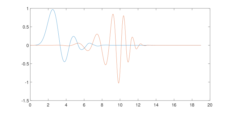
Figure 1: Father (blue) and mother (red) Daubechies wavelets with order $N=10$.

3.2 General model and theoretical assumptions

Without loss of generality, we will considered three exogenous $\mathcal{B}_{\infty,\infty}^{0}\left([0,1]\right)$-valued variables (i.e., $b=3$). According to the theoretical model presented in (5), and considering the function spaces defined in (LABEL:eqfss), the following ARBX(1) process has been generated:

$$\overline{X}_{n} = \overline{\rho}\left(\overline{X}_{n-1}\right)+\overline{\varepsilon}_{n},\quad{\color[rgb]{0,0,1}\overline{X}_{n},~{}\overline{\varepsilon}_{n}\in\overline{B}},\quad n\in\mathbb{Z},$$

$$\overline{X}_{n} = \begin{pmatrix}X_{n}\\ Z_{n+1,1}\\ Z_{n+1,2}\\ Z_{n+1,3}\end{pmatrix},\quad\overline{\varepsilon}_{n}=\begin{pmatrix}\varepsilon_{n}\\ \eta_{n,1}\\ \eta_{n,2}\\ \eta_{n,3}\end{pmatrix},\quad\overline{\rho}=\begin{pmatrix}\rho&a_{1}&a_{2}&a_{3}\\ \mathbf{0}_{B}&u_{1}&\mathbf{0}_{B}&\mathbf{0}_{B}\\ \mathbf{0}_{B}&\mathbf{0}_{B}&u_{2}&\mathbf{0}_{B}\\ \mathbf{0}_{B}&\mathbf{0}_{B}&\mathbf{0}_{B}&u_{3}\end{pmatrix},\quad{\color[rgb]{0,0,1}X_{n}\in\mathcal{B}_{\infty,\infty}^{0}\left([0,1]\right)},$$

where $Z_{n,i},~{}\eta_{n,i}$ are also valued in $B=\mathcal{B}_{\infty,\infty}^{0}\left([0,1]\right)$, for each $n\in\mathbb{Z}$ and $i=1,2,3$.

As discussed in (RuizAlvarez18_JMVA, , Section 6), and from the embeddings results in Triebel83 ,

$$\mathcal{H}(X)=H_{2}^{\gamma}\left([0,1]\right)\hookrightarrow H_{2}^{\beta}\left([0,1]\right)\hookrightarrow\mathcal{B}_{1,1}^{0}\left([0,1]\right)\hookrightarrow H=L^{2}\left([0,1]\right)\hookrightarrow\mathcal{B}_{\infty,\infty}^{0}\left([0,1]\right),$$

satisfying Assumptions A4–A5 for the case $b=1$, as long as $\gamma>2\beta>1$, being $\mathcal{H}(X)$ the Reproducing Kernel Hilbert space generated by the covariance operator $C=\left(I-\Delta\right)^{-\gamma}$ (the $2\gamma/\beta$ power of the Bessel potential of order $\beta$ restricted to $L^{2}\left([0,1]\right)$. Since the Cartesian product preserves the continuous embeddings, Assumptions A4–A5 are directly verified as long as

$$\beta>1/2,\quad\gamma_{i}>2\beta,\quad i=1,2,3,4.$$

Note that, since $\widetilde{\overline{H}}^{\ast}=\left[H_{2}^{\beta}\left([0,1]\right)\right]^{4}$, the smaller is the parameter $\beta$, the smaller local regularity is observed in our curves. Henceforth, $\beta=3/5>1/2$ is fixed to illustrate our framework in one of the most irregular scenarios. Concerning $\left\{\gamma_{i},\ i=1,2,3,4\right\}$, we exposed that $\gamma_{i}>2\beta$ is just required, for each $i=1,2,3,4$. See Remark 1 below.

Remark 1

Since $\left\{X_{n},\ n\in\mathbb{Z}\right\}$ constitutes our endogenous variable of interest to be predicted, for simplicity, it seems reasonable to suppose that $\gamma_{1}<\gamma_{i}$, for each $i=2,3,4$; that is, exogenous functional random variables (auxiliary external information) are rather regular than the exogenous variables to be predicted. Hence, the following parametric family of values, in terms of monotonic increasing functions, will be considered in the numerical results in Section 4:

$$\gamma^{1}=\left\{\gamma_{i}=2\beta+\frac{i}{10},\ i=1,\ldots,b+1\right\},\quad\gamma^{2}=\left\{\gamma_{i}=2\beta+\log_{10}\left(i+1\right),\ i=1,\ldots,b+1\right\}.$$ (15)

Note that $\gamma^{2}$ will provide more regular curves. From a theoretical point of view, note that each parametric family

$$\gamma=\left\{\gamma_{i}=2\beta+f(i),\ i=1,\ldots,b\right\},\quad f(i)>0,~{}i=1,\ldots,b+1,$$

could be adopted.

3.2.1 Covariance structures

In relation to the covariance structure of the model in (LABEL:general_model), and in order to ensure the first part of Assumption A1, a truncated version, on a multidimensional finite interval, of the following multivariate infinite-dimensional Gaussian measures in $\overline{H}=H^{4}$ will be generated:

$$\overline{X}_{0}=\begin{pmatrix}X_{0}\\ Z_{1,1}\\ Z_{1,2}\\ Z_{1,3}\end{pmatrix}\sim\mathcal{N}\left(\mathbf{0},\overline{C}\right),\quad\overline{\varepsilon}_{0}=\begin{pmatrix}\varepsilon_{0}\\ \eta_{0,1}\\ \eta_{0,2}\\ \eta_{0,3}\end{pmatrix}\sim\mathcal{N}\left(\mathbf{0},\overline{C}_{\boldsymbol{\eta}}\right),$$ (16)

where

$$\overline{C} = \begin{pmatrix}C_{X_{0},X_{0}}&C_{X_{0},Z_{1,1}}&C_{X_{0},Z_{1,2}}&C_{X_{0},Z_{1,3}}\\ C_{Z_{1,1},X_{0}}&C_{Z_{1,1},Z_{1,1}}&C_{Z_{1,1},Z_{1,2}}&C_{Z_{1,1},Z_{1,3}}\\ C_{Z_{1,2},X_{0}}&C_{Z_{1,2},Z_{1,1}}&C_{Z_{1,2},Z_{1,2}}&C_{Z_{1,2},Z_{1,3}}\\ C_{Z_{1,3},X_{0}}&C_{Z_{1,3},Z_{1,1}}&C_{Z_{1,3},Z_{1,2}}&C_{Z_{1,3},Z_{1,3}}\end{pmatrix},$$ (17)

and

$$\overline{C}_{\boldsymbol{\eta}} = \begin{pmatrix}C_{\varepsilon_{0},\varepsilon_{0}}&C_{\varepsilon_{0},\eta_{0,1}}&C_{\varepsilon_{0},\eta_{0,2}}&C_{\varepsilon_{0},\eta_{0,3}}\\ C_{\eta_{0,1},\varepsilon_{0}}&C_{\eta_{0,1},\eta_{0,1}}&C_{\eta_{0,1},\eta_{0,2}}&C_{\eta_{0,1},\eta_{0,3}}\\ C_{\eta_{0,2},\varepsilon_{0}}&C_{\eta_{0,2},\eta_{0,1}}&C_{\eta_{0,2},\eta_{0,2}}&C_{\eta_{0,2},\eta_{0,3}}\\ C_{\eta_{0,3},\varepsilon_{0}}&C_{\eta_{0,3},\eta_{0,1}}&C_{\eta_{0,3},\eta_{0,2}}&C_{\eta_{0,3},\eta_{0,3}}\end{pmatrix}.$$ (18)

In equation (17), we have denoted

$$C_{X_{0},X_{0}}=\left(I-\Delta\right)^{-\gamma_{1}},\quad C_{Z_{1,i},Z_{1,i}}={\rm E}[Z_{1,i}\otimes Z_{1,i}]=\left(I-\Delta\right)^{-\gamma_{i}},~{}i=1,2,3,$$ (19)

with $\left(I-\Delta\right)^{-\gamma}$ being the Bessel potential of order $2\gamma,$ and $C_{Z_{1,i},X_{0}}={\rm E}[Z_{1,i}\otimes X_{0}]$ and $C_{X_{0},Z_{1,i}}={\rm E}[X_{0}\otimes Z_{1,i}]$, for $i,l=1,2,3.$ The functional entries of (17) are now explicitly defined, ensuring, in particular, the one–dimensionality of their eigenspaces, in order to get the second part of Assumption A1 to hold. Furthermore, for every $f\in L^{2}([0,1]),$ and for $i,l=1,2,3,$

$$C_{X_{0},X_{0}}\left(f\right) = \displaystyle\sum_{j=1}^{\infty}(1+j)^{-\gamma_{1}}\langle\phi_{j},f\rangle_{H}\phi_{j},$$

$$C_{X_{0},Z_{1,i}}\left(f\right) = \displaystyle\sum_{j=1}^{\infty}(1+j)^{-\frac{\gamma_{1}+\gamma_{i+1}}{2}}\langle\phi_{j},f\rangle_{H}\phi_{j},$$

$$C_{Z_{1,i},X_{0}}\left(f\right) = \displaystyle\sum_{j=1}^{\infty}(1+j)^{-\frac{\gamma_{1}+\gamma_{i+1}}{2}}\langle\phi_{j},f\rangle_{H}\phi_{j},$$

$$C_{Z_{1,l},Z_{1,i}}\left(f\right) = \displaystyle\sum_{j=1}^{\infty}(1+j)^{-\frac{\gamma_{l}+\gamma_{i+1}}{2}}\langle\phi_{j},f\rangle_{H}\phi_{j},$$

Henceforth, the following basis will be adopted, in the decompositions exposed in (LABEL:covar_oper):

$$\phi_{j}\left(x\right)=\sqrt{\frac{2}{b-a}}{\rm sin}\left(\frac{\pi jx}{b-a}\right),\quad j\geq 1,\quad x\in\left[a,b\right],\quad a=0,\ b=1.$$ (21)

That is, the smoother functional values of the exogenous random variables are extended to the space $H=L^{2}([0,1]),$ by projection into the elements of the basis in (21). Adopting as an example the parametric family $\gamma^{1}$ displayed in (15), the functional entries $C_{X_{0},X_{0}}$ and $C_{Z_{0,3},Z_{0,3}}$ are represented in Figure, 2 below.

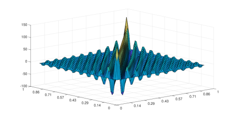
Figure 2: Covariance kernels defining $C_{X_{0},X_{0}}$ (on left) and $C_{Z_{1,3},Z_{1,3}}$ (on right), generated in terms of $\gamma_{1}=2\beta+1/10$ and $\gamma_{4}=2\beta+4/10$ with $\beta=3/5$, respectively, plotted with a discretization step size $\Delta h=0.0159$.

In the same way, the functional entries of (18) are explicitly defined as follows:

$$C_{\varepsilon_{0},\varepsilon_{0}}={\rm E}\left[\varepsilon_{0}\otimes\varepsilon_{0}\right],\quad C_{\eta_{0,i},\eta_{0,l}}={\rm E}\left[\eta_{0,i}\otimes\eta_{0,l}\right],\ i,l=1,2,3$$

$$C_{\eta_{0,i},\varepsilon_{0}}={\rm E}\left[\eta_{0,i}\otimes\varepsilon_{0}\right],\quad C_{\varepsilon_{0},\eta_{0,i}}={\rm E}\left[\varepsilon_{0}\otimes\eta_{0,i}\right],\ i=1,2,3.$$ (22)

In particular, and for simplifications purposes, we have considered, in the generations, $C_{\eta_{0,i},\eta_{0,l}}=C_{\varepsilon_{0},\eta_{0,i}}=\mathbf{0}_{H},$ $i,l=1,2,3,$ $i\neq l.$ The following identities characterise the diagonal functional entries of $\overline{C}_{\boldsymbol{\eta}},$ in terms of the elements of the basis $\{\phi_{j},\ j\geq 1\}$ introduced in equation (21): For $i=1,2,3,$ and $j,h\geq 1,$

$$\langle C_{\varepsilon_{0},\varepsilon_{0}}(\phi_{j}),\phi_{h}\rangle_{H} = \begin{cases}C_{X_{0}X_{0}}(\phi_{j})(\phi_{j})(1-[\rho(\phi_{j})(\phi_{j})]^{2})\quad&j=h,\\ e^{-\left|j-h\right|^{2}/W^{2}}\quad&j\neq h\end{cases},$$

$$\langle C_{\eta_{0,i},\eta_{0,i}}(\phi_{j}),\phi_{h}\rangle_{H} = \begin{cases}C_{Z_{0,i},Z_{0,i}}(\phi_{j})(\phi_{j})\left(1-[u_{i}(\phi_{j})(\phi_{j})]^{2}\right)\quad&j=h\\ e^{-\left|j-h\right|^{3}/W^{2}}\quad&j\neq h\end{cases},$$

where, for $i=1,2,3,$ and $j,h\geq 1,$ considering $W=0.4,$

$$\rho(\phi_{j})(\phi_{h})=\langle\rho(\phi_{j}),\phi_{h}\rangle_{H} = \begin{cases}(1+j)^{-1.5}\quad&j=h,\\ e^{-\left|j-h\right|/W}\quad&j\neq h\end{cases},$$

$$u_{i}(\phi_{j})(\phi_{h})=\langle u_{i}(\phi_{j}),\phi_{h}\rangle_{H} = \begin{cases}(1+j)^{-(3+0.5i)}\quad&j=h,\\ e^{-\left|j-h\right|^{2}/W}\quad&j\neq h.\end{cases}$$ (23)

Furthermore, for $i=1,2,3,$ and $j,h\geq 1,$

$$\langle a_{i}(\phi_{j}),\phi_{h}\rangle_{H}=\begin{cases}(1+j)^{-(4+0.5i)}\quad j=h,\\ e^{-\left|j-h\right|^{3}/W}\quad j\neq h\end{cases}.$$ (24)

4 Simulation study

There is a twofold objective for the numerical results displayed in this Section: firstly, to illustrate the strong consistency of the ARBX(1) plug-in predictor for an increasing sequence of sample sizes and, secondly, to explore whether our ARBX(1) prediction methodology is sensitive to the number of grid points for a decreasing (to zero) sequence of discretization steps.

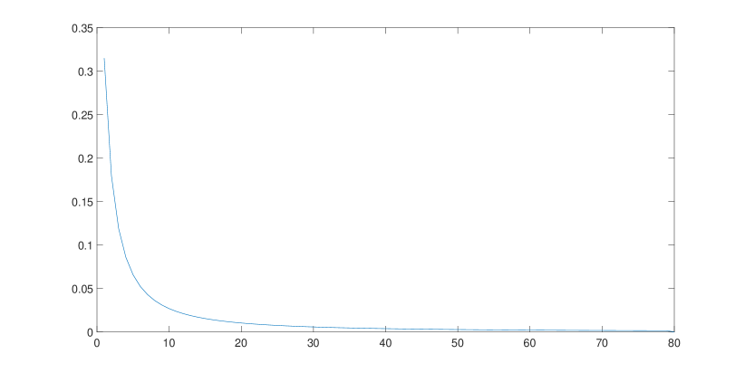
Figure 12: Values of $\displaystyle\left\|\overline{\rho}\left(\cdot\right)-\displaystyle\sum_{l=1}^{K}\langle\overline{\rho}\left(\cdot\right),\overline{\phi}_{j}\rangle_{\left[\mathcal{B}_{2,2}^{-\beta}([0,1])\right]^{b+1}}\overline{\phi}_{j}\right\|_{\mathcal{L}\left([\mathcal{B}_{\infty,\infty}([0,1])]^{b+1}\right)},$ for $K$–values reflected in the horizontal axis.

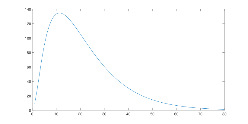
Figure 13: Values of $\frac{k_{n}C_{k_{n}}^{-1}\displaystyle\sum_{j=1}^{k_{n}}a_{j}}{\sqrt{n/\ln(n)}},$ considering $k_{n}=\left[\ln(n)\right]^{-},$ for $k_{n}$-values reflected in the horizontal axis.

As given in Section 2, the componentwise estimator (8) of $\overline{\rho}$ is strongly consistent in $\mathcal{L}(\overline{B}),$ under the formulated Assumptions A1–A5, and the conditions in (RuizAlvarez18_JMVA, , Lemma 8–9). The general model proposed in Section 3 has been demonstrated to satisfy the theoretical conditions included in Assumption A1 and Assumptions A4–A5. Regarding empirical conditions displayed in Assumptions A2–A3, for a given functional sample size $n$, in the following, we will consider $k_{n}=[\ln(n)]^{-},$ where $[\cdot]^{-}$ denotes the integer part function. This truncation parameter ensures that, for all the sample sizes studied, the empirical eigenvalue $C_{n,k_{n}}$ is positive, and therefore, Assumption A2 is satisfied. See Figures 12–13 in the Appendix for checking how Assumption A3 and extra condition required in (RuizAlvarez18_JMVA, , Theorem 1) are respectively satisfied.

4.1 Strong consistency of the ARBX(1) plug–in predictor

As commented, and aimed at illustrating the behaviour of our plug–in predictor for very large sample sizes, let us consider in this Section the following increasing sequence of sample sizes:

$$n=\left[n_{1},\ldots,n_{9}\right]=\left[1500,2500,5000,15000,25000,50000,75000,100000,130000\right]$$

Some trajectories of $X_{n}^{\star}\in\widetilde{H}^{\star}=\mathcal{B}^{\beta}_{2,2}([0,1])$ have been plotted in Figure 3 below, adopting a discretization step $\Delta h=0.0159$, just smoothing with cubicspline option of fit.m MatLab function.

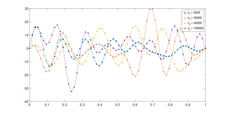
Figure 3: Functional values of $X_{n}^{\star}$ at $n=5000,25000,50000,100000$, with discretization step size $\Delta h=0.0159$.

As noted, we have adopted $k_{n}=[\ln(n)]^{-}$ as truncation parameter, such that, according to (RuizAlvarez18_JMVA, , Theorem 1), the strong-consistency of the componentwise estimator (8) in $\mathcal{L}(\overline{B})$ follows when

$$k_{n}C_{k_{n}}^{-1}\sum_{j=1}^{k_{n}}a_{j}=o\left(\sqrt{n/\ln(n)}\right),\quad n\to\infty,$$ (25)

where

$$a_{1}=\frac{2\sqrt{2}}{C_{1}-C_{2}};\ a_{j}=2\sqrt{2}\max\left(\frac{1}{C_{j-1}-C_{j}},\frac{1}{C_{j}-C_{j+1}}\right),\quad j\geq 2.$$

As before, $\{C_{j},\ j\geq 1\}$ denotes the system of eigenvalues of the extended matrix autocovariance operator $\overline{C}$ in (17). We can observe in Figure 13 in the Appendix that condition (25) is satisfied.

For numerically proving the strong consistency of the ARBX(1) plug–in predictor, note that the upper bound derived in (RuizAlvarez18_JMVA, , Theorem 1 and Corollary 1), for the $\overline{B}$–norm of the functional error, $\left\|\overline{\rho}(\overline{X}_{n})-\widehat{\overline{X}}_{n}\right\|_{\overline{B}},$ ensuring strong consistency of the plug–in predictor in $\overline{B},$ is given by

$$\mathcal{M}(\omega)\xi_{n}=\mathcal{M}(\omega)\exp\left(\frac{-n}{C_{k_{n}}^{-2}k_{n}^{2}\left(\displaystyle\sum_{j=1}^{k_{n}}a_{j}\right)^{2}}\right),$$ (26)

where $\mathcal{M}(\omega)=\|\overline{X}_{0}(\omega)\|_{\overline{B}},$ $\omega\in\Omega,$ and for each functional sample size $n,$ as before, $C_{k_{n}}$ is the $k_{n}$–th eigenvalue of the extended autocovariance operator $\overline{C}$ in (17). Hence, Table 1 reflects the percentage of simulations in which the error $\overline{B}$–norm is greater than the upper bound in (26), for each one of the parametric families of $\gamma$ defined in (15).

Table 1: Percentage of simulations from the $200$ generations of each sample size, where the error $\overline{B}$–norm is larger than the upper bound (26). The sample sizes $n=1500,2500,5000,15000,25000,50000,75000,100000,130000$ have been tested. The truncation rule $k_{n}=\left[\ln(n)\right]^{-}$ has been adopted. Two parametric families $\gamma^{1}$ and $\gamma^{2}$ have been adopted for the generation of covariance operators (see equation (15)).

$n_{t}$	$\gamma^{1}$	$\gamma^{2}$
$n_{1}=1500$	$11.5~{}\%$ ($\frac{23}{200}$)	$12~{}\%$ ($\frac{24}{200}$)
$n_{2}=2500$	$9.5~{}\%$ ($\frac{19}{200}$)	$9~{}\%$ ($\frac{18}{200}$)
$n_{3}=5000$	$8~{}\%$ ($\frac{16}{200}$)	$8.5~{}\%$ ($\frac{17}{200}$)
$n_{4}=15000$	$4.5~{}\%$ ($\frac{9}{200}$)	$4.5~{}\%$ ($\frac{9}{200}$)
$n_{5}=25000$	$3.5~{}\%$ ($\frac{7}{200}$)	$2.5~{}\%$ ($\frac{5}{200}$)
$n_{6}=50000$	$2.5~{}\%$ ($\frac{5}{200}$)	$1.5~{}\%$ ($\frac{3}{200}$)
$n_{7}=75000$	$2~{}\%$ ($\frac{4}{200}$)	$1~{}\%$ ($\frac{2}{200}$)
$n_{8}=100000$	$1~{}\%$ ($\frac{2}{200}$)	$0.5~{}\%$ ($\frac{1}{200}$)
$n_{9}=130000$	$0~{}\%$ ($\frac{0}{200}$)	$0~{}\%$ ($\frac{0}{200}$)

4.2 Asymptotic behaviour of discretely observed ARBX(1) processes

The previous subsection was intended to numerically illustrate the strong consistency of ARBX(1) plug–in predictor, focusing on its behaviour when $n\to\infty$, for a fixed discretization step in the generation of both trajectories and wavelets. In contrast, the main aim of this subsection is to explore the sensitiveness of the above ARBX(1) prediction methodology to the discretization step size. Here, we provide the reader a brief numerical study about what is going on when sample sizes are not too large ($n$ does not tend to infinite) but the discretization step adopting for the generation of the trajectories tends to zero ($\Delta h\to 0$).

For this purpose, the set $\left\{\Delta h_{j}=\frac{1}{3^{2+j}},\ j=1,\ldots,7\right\}$ of decreasing (to zero) discretization steps are analysed (see Figure 4 below):

$$\Delta h_{1} = 3.70(10^{-2}),\quad\Delta h_{2}=1.23(10^{-2}),\quad\Delta h_{3}=4.12(10^{-3}),\quad\Delta h_{4}=1.37(10^{-3}),$$

$$\Delta h_{5} = 4.57(10^{-4}),\quad\Delta h_{6}=1.52(10^{-4}),\quad\Delta h_{7}=5.08(10^{-5}),$$

such that $\left\{3^{2+j}+1,\ j=1,\ldots,7\right\}$ grid points are respectively considered.

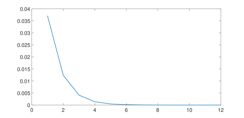
Figure 4: Discretization steps $\Delta h_{j}=\frac{1}{3^{2+j}}$, for $j=1,\ldots,12$, displaying that $\Delta h_{j}\to 0$ as $j\to\infty$.

Now, only sample sizes $n=\left[n_{1},n_{2},n_{3}\right]=[5000,15000,30000]$ have been considered. As below, Table 2 reflects the percentages of simulations in which the error $B$–norm is larger than the upper bound in (26), for each discretization step size, functional sample size and parametric families $\gamma^{1}$ and $\gamma^{2}$.

Table 2: Percentage of simulations from the $200$ generations of each sample size, where the error $\overline{B}$–norm is larger than the upper bound (26). The sample sizes $n=5000,15000,30000$ have been tested. The truncation rule $k_{n}=\left[\ln(n)\right]^{-}$ has been adopted. Two parametric families $\gamma^{1}$ and $\gamma^{2}$ have been adopted for the generation of covariance operators (see equation (15)). Discretization steps $\left\{\Delta h_{j}=3^{-(2+j)},\ j=1,\ldots,7\right\}$ are adopted.

	$\gamma^{1}$			$\gamma^{2}$
$n\longrightarrow$	$5000$	$15000$	$30000$	$5000$	$15000$	$30000$
$\Delta h_{1}$	$12~{}\%$ ($\frac{24}{200}$)	$10~{}\%$ ($\frac{20}{200}$)	$7.5~{}\%$ ($\frac{15}{200}$)	$13.5~{}\%$ ($\frac{27}{200}$)	$10.5~{}\%$ ($\frac{21}{200}$)	$6.5~{}\%$ ($\frac{13}{200}$)
$\Delta h_{2}$	$9~{}\%$ ($\frac{18}{200}$)	$5.5~{}\%$ ($\frac{11}{200}$)	$4~{}\%$ ($\frac{8}{200}$)	$9.5~{}\%$ ($\frac{19}{200}$)	$6~{}\%$ ($\frac{12}{200}$)	$4~{}\%$ ($\frac{8}{200}$)
$\Delta h_{3}$	$7~{}\%$ ($\frac{14}{200}$)	$4~{}\%$ ($\frac{8}{200}$)	$3.5~{}\%$ ($\frac{7}{200}$)	$7.5~{}\%$ ($\frac{15}{200}$)	$4~{}\%$ ($\frac{8}{200}$)	$3~{}\%$ ($\frac{6}{200}$)
$\Delta h_{4}$	$5.5~{}\%$ ($\frac{11}{200}$)	$3.5~{}\%$ ($\frac{7}{200}$)	$2~{}\%$ ($\frac{4}{200}$)	$4.5~{}\%$ ($\frac{9}{200}$)	$2.5~{}\%$ ($\frac{5}{200}$)	$2~{}\%$ ($\frac{4}{200}$)
$\Delta h_{5}$	$2.5~{}\%$ ($\frac{5}{200}$)	$1.5~{}\%$ ($\frac{3}{200}$)	$1~{}\%$ ($\frac{2}{200}$)	$1.5~{}\%$ ($\frac{3}{200}$)	$1~{}\%$ ($\frac{2}{200}$)	$1~{}\%$ ($\frac{2}{200}$)
$\Delta h_{6}$	$1.5~{}\%$ ($\frac{3}{200}$)	$0.5~{}\%$ ($\frac{1}{200}$)	$0.5~{}\%$ ($\frac{1}{200}$)	$1~{}\%$ ($\frac{2}{200}$)	$0.5~{}\%$ ($\frac{1}{200}$)	$0~{}\%$ ($\frac{0}{200}$)
$\Delta h_{7}$	$1~{}\%$ ($\frac{2}{200}$)	$0.5~{}\%$ ($\frac{1}{200}$)	$0~{}\%$ ($\frac{0}{200}$)	$0.5~{}\%$ ($\frac{1}{200}$)	$0~{}\%$ ($\frac{0}{200}$)	$0~{}\%$ ($\frac{0}{200}$)

In the light of the results displayed in Tables 1–2, our ARBX(1) plug–in predictor is strongly consistent, either considering sample sizes tending to infinite or considering discretely observed ARBX(1) process adopting a discretization step converging to zero.

5 Real-data application: short–term forecasting of air pollutants

In this section, the performance of the ARBX(1) based prediction approach here presented is illustrated in a real–data example. Specifically, the short–term forecasting of daily average concentrations of atmospheric aerosol particles with diameters less than 10 $\mu m$, also known as PM₁₀ (coarse particles), is achieved from a functional perspective. The importance of the accurate forecasting of this kind of particles relies on the fact that they are inhalable atmospheric pollution particles, which impact the public health. Following the suggestions by the World Health Organization, the European Union developed in 2008 (in particular, directive 2008/50/EU) a complete legislative package, establishing health based standards for the levels of PM₁₀: daily mean concentration of PM₁₀ should not be greater than $50~{}\mu g~{}m^{-3}$ more than 35 days per year, neither the annual average of concentration of PM₁₀ shall not be greater than $40~{}\mu g~{}m^{-3}$. However, this limit has been exceed during the last years in heavily industrialized areas, deriving in severe people’s health problems. Therefore, PM₁₀ forecasting is crucial to adopting efficient public transport policies. The dataset is analysed in Section 5.1, while Section 5.2 describes the preprocessing procedure required, before implementing our functional prediction methodology in Section 5.3.

5.1 Dataset description

The dataset considered is comprised of daily average concentrations of PM₁₀, coming from hourly measurements, from January 1, 2007 to March 31, 2011, collected by the air quality Normand (French) authority, known as Air Normand. This dataset is freely available in the website http://www.atmonormandie.fr. Specifically, we pay attention to $6$ of the $13$ fixed pollution monitoring stations network located throughout Haute–Normandie region, considered one of the most heavily industrialized areas in France (see locations in the map displayed in Figure 5).

Figure 5: On left: map (extracted from Google Maps) displaying the location of the six pollution monitoring stations analysed. On right: enlarged map displaying the stations near Rouen.

In the following, as shown in the map below, these monitoring stations will be denoted as $\left\{S_{c},\ c=1,\ldots,6\right\}$, selected with the aim of reflecting a wide variety of scenarios, such that roadisdes (stations S2 and S5), urban areas (stations S1 and S4), industrial zones (station S5) and rural regions (station S6). As reflected in Figure 6 below (see also descriptive statistics reflected in Table 3 in the Appendix), the monitoring station $S_{6}$ (rural area) has registered the smallest PM₁₀ concentrations, while stations $S_{2}$ and $S_{5}$ (roadsides) display the highest pollution levels. These stations also display the highest variability, which seems logical since pollution levels in roadside are strongly dependent on traffic jams.

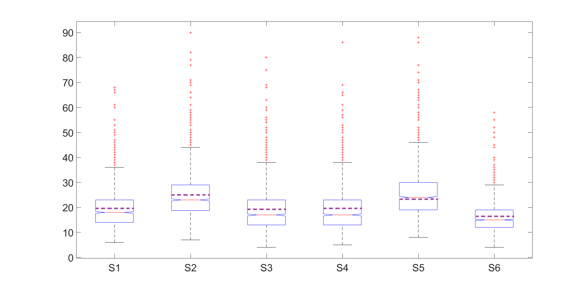
Figure 6: Boxplots on the samples of the PM₁₀ concentrations ($\mu g~{}m^{-3}$). Purple dotted lines reflect the average concentrations, while red solid lines splitting the box reflect the medians.

The ARBX(1) modelling is adopted since pollution particles are mainly procured from natural sources (i.e., influenced by meteorological variables), or due to human activity. In our study we incorporate the exogenous information coming from meteorological variables. Specifically, we consider the following four exogenous variables ($b=4$ in our ARBX(1) model): daily average temperature (${}^{\circ}C$), daily average atmospheric pressure ($hPa$), daily average wind speed ($ms^{-1}$), and daily maximum gradient of temperature (${}^{\circ}C$), computed all of them from hourly measurements. Note that daily maximum gradient of temperature denotes the daily maximum of the hourly differences between the temperature at $2$ and $100$ meters. Wind speed is commonly included jointly with wind direction. However, this aspect would require an spatial correlation structure for the stations, which is out of the scope of the current article. Some discussion about how the spatial extension can be implemented can be found in Section 6.

Measurements of these meteorological variables were collected at three meteorological stations belonging to the French national meteorological service, such that each air pollution station is associated with the closest meteorological station. Thus, pollution stations $S_{1},S_{2}$ and $S_{3}$ are associated to a common meteorological station. Also, a second meteorological station covers the pollution stations $S_{4}$ and $S_{5}.$ Finally, a third meteorological station is associated with the pollution station $S_{6}.$ Figure 7 displays boxplots for all of these measurements collected in the three meteorological stations available (see also Table 4 in the Appendix, displaying basic descriptive statistics about them). As commented, pollution monitoring stations are separately analysed, and no spatial interaction is contemplated.

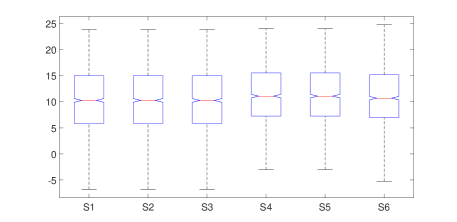
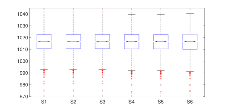
Figure 7: Boxplots reflecting the sample behaviour of exogenous variables at each meteorological station (mean temperature on the top left, mean wind speed on the top right, mean air pressure at the bottom left and maximum temperature gradient at the bottom right), associated with pollution stations $\left(S_{1},~{}S_{2},~{}S_{3}\right)$, $\left(S_{4},~{}S_{5}\right)$ and $\left(S_{6}\right)$.

5.2 Data preprocessing

To obtain our functional dataset the following steps are implemented:

Step 1: Missing–data imputation. As can be checked in Table 3 below, missing values appeared: an imputation procedure is required. Taking the more powerful R package as a reference (see Moritz17 ; MoritzBartz17 ), we have implemented one of the imputation methods there described, assigning to missing values an average of previous and posterior non missing values. This choice has been adopted for preserving the dependence structure of data. Since pollution data is strongly linked with routines and consumption patterns in business days, the past and the next five values are considered. At each station, $1551$ records are then available. Daily observations of the endogenous variable at station $S_{1}$ are displayed after imputation in Figure 8.

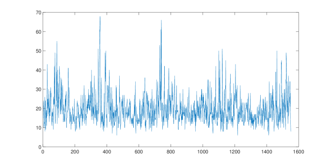
Figure 8: Daily observations (from 01/01/2007 to 31/03/2011) at station $S_{1}$ after imputation.

Step 2: Fitting to $\boldsymbol{31}$–days standard months. As can be appreciated in the previous sections, our functional data should be evaluated in the same function spaces; that is, exogenous and endogenous functional variables should be valued in the same Banach space. In this way, aimed at achieving balanced data for each of the stations, we need that all months (i.e., all intervals) contain the same amount of days (i.e., the same amount of grid points). For this purpose, Cubicspline option in fit.m MatLab function has been applied, obtaining $31$ measurements per month: an unique grid of $31\times 51=1581$ points is considered for each of exogenous and endogenous variables, at each station.

Step 3: Splitting our dataset. At each pollution station $S_{c},$ $c=1,\dots,6,$ we will construct our plug–in predictor $\widehat{\overline{X}}_{50}^{c}=\widetilde{\overline{\rho}}_{k_{n}}(\overline{X}_{49}^{c}),$ from a functional sample $\{\overline{X}_{0},\dots,\overline{X}_{49}\}$ of size $50.$ Thus, functional prediction is achieved for the last month, March, 2011, at each pollution station.

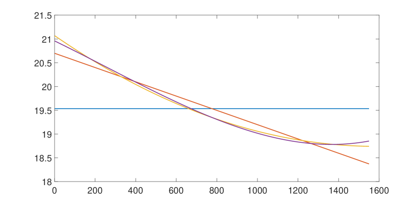
Figure 14: Fitting trends as polynomial of degrees $0$ (null trend; blue line), $1$ (linear trend; red line), $2$ (quadratic trend; yellow line) and $3$ (cubic trend; purple line).

Step 4: Detrending and deseasonalizing. As usual, a polynomial trend $a_{0}+a_{1}t+a_{2}t^{2}+a_{3}t^{3}+...$ will be fitted for detrending all the curve data. Thus, we have checked the trends fitting polynomials of increasing degree, stopping when the fitting trends between two successive degrees display a similar behaviour. As shown in Figure 14 in the Appendix, and applying the law of parsimony, a polynomial quadratic trend $a_{0}+a_{1}t+a_{2}t^{2}$ has finally been fitted (based on a functional sample of size $50$) for detrending all the curve data, including the last month. After detrending, annual seasonality is also removed.

Step 5: Modelling by an ARBX(1) process. Summarizing, from the previous steps, our functional sample is constituted by $50$ detrended, and annually deseasonalized observed curves for the endogenous and exogenous variables (on a grid of $1581$ points). Plug–in functional prediction is achieved for the $51$–th month, from the observed curves at the previous $50$ months by fitting ARBX(1) model in equation (28) below. Figure 9 displays our PM₁₀ functional dataset at station $S_{1},$ corresponding to the period January 2007–February 2011.

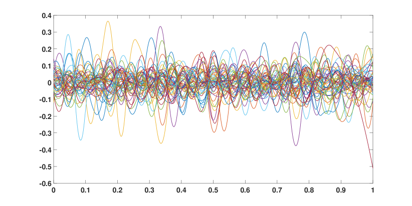
Figure 9: Observed PM₁₀ curves at stations $S_{1}$ for the period January 2007–February 2011.

Specifically, the following ARBX(1) model is fitted:

$$\overline{X}_{n}^{c}=\overline{\rho}^{c}\left(\overline{X}_{n-1}^{c}\right)+\overline{\varepsilon}_{n}^{c},\quad n=0,1,\ldots,T=49,\quad c=1,\ldots,6,$$ (27)

where $b=4,$ and hence,

$$\overline{X}_{n}^{c}=\begin{pmatrix}X_{n}^{c}\\ Z_{n+1,1}^{c}\\ Z_{n+1,2}^{c}\\ Z_{n+1,3}^{c}\\ Z_{n+1,4}^{c}\end{pmatrix},\quad\overline{\varepsilon}_{n}^{c}=\begin{pmatrix}\varepsilon_{n}^{c}\\ \eta_{n,1}^{c}\\ \eta_{n,2}^{c}\\ \eta_{n,3}^{c}\\ \eta_{n,4}^{c}\end{pmatrix},\quad\overline{\rho}^{c}=\begin{pmatrix}\rho^{c}&a_{1}^{c}&a_{2}^{c}&a_{3}^{c}&a_{4}^{c}\\ \mathbf{0}_{B}&u_{1}^{c}&\mathbf{0}_{B}&\mathbf{0}_{B}&\mathbf{0}_{B}\\ \mathbf{0}_{B}&\mathbf{0}_{B}&u_{2}^{c}&\mathbf{0}_{B}&\mathbf{0}_{B}\\ \mathbf{0}_{B}&\mathbf{0}_{B}&\mathbf{0}_{B}&u_{3}^{c}&\mathbf{0}_{B}\\ \mathbf{0}_{B}&\mathbf{0}_{B}&\mathbf{0}_{B}&\mathbf{0}_{B}&u_{4}^{c}\end{pmatrix},\quad c=1,\ldots,6.$$ (28)

Equivalently, for $c=1,\ldots,6,$

$$X_{n}^{c}=\rho^{c}\left(X_{n-1}^{c}\right)+\displaystyle\sum_{i=1}^{4}a_{i}^{c}\left(Z_{n,i}^{c}\right)+\varepsilon_{n}^{c},\quad n=0,1,\ldots,T=49,$$ (29)

with, for $i=1,\dots,4,$ $a_{i}^{c}\in\mathcal{L}(B),$ $\rho^{c}\in\mathcal{L}(B),$ and

$$Z_{n,i}^{c}=u_{i}^{c}\left(Z_{n-1,i}^{c}\right)+\eta_{n,i}^{c},\quad u_{i}^{c}\in\mathcal{L}(B),\quad n=0,1,\ldots,T=49.$$ (30)

It can be observed in Figure 9 that PM₁₀ curves are continuous. Hence, $\beta>1/2.$ As before, we look for the minimal local regularity order, in our fitting of the previous introduced ARBX(1) model, with $b=4.$ Thus, the parameter values $\beta=3/5$ and $\gamma=\gamma_{i}=2\beta+\epsilon,$ with $\epsilon=0.01,$ $i=1,2,3,4,$ have been considered in the definition of our function space scenario, given by

$$\overline{B}=\left[\mathcal{B}_{\infty,\infty}^{0}\left([0,1]\right)\right]^{5},\ \widetilde{\overline{H}}=\left[\mathcal{B}_{2,2}^{-\beta}\left([0,1]\right)\right]^{5},\ \overline{H}=[L^{2}([0,1])]^{5},\ \mathcal{H}(\overline{X})=[\mathcal{B}^{\gamma}_{2,2}\left([0,1]\right)]^{5}.$$ (31)

5.3 The performance of the ARBX(1) plug–in predictor

In the implementation of the leave–one–out cross validation procedure, at each pollution station $S_{c},$ $c=1,\dots,6,$ the following functional sample is considered:

$$\overline{Y}^{h,c} = \left\{\overline{Y}_{i}^{h,c},\quad i=0,1,\ldots,47\right\}=\left\{\overline{X}_{i}^{c},\quad i=0,1,\ldots,48\right\}\setminus\left\{\overline{X}_{h}^{c}\right\},$$

by removing the functional data $\overline{X}_{h}^{c},$ $h=0,1,\ldots,48,$ as well as the functional data $\overline{X}_{49}^{c},$ $c=1,\dots,6,$ in the computation of the componentwise estimator (8) of the autocorrelation operator $\overline{\rho}.$ Thus, at each iteration $h\in\{0,1,\ldots,48\}$ of the implemented leave–one–out cross validation procedure, the ARBX(1) plug–in predictor $[\widehat{\overline{X}}_{50}^{c}]_{h,k_{n}}$ of $\overline{X}_{50}^{c}$ is computed, from a functional sample of size $48,$ considering the truncation order $k_{n},$ as follows

$$[\widehat{\overline{X}}_{50}^{c}]_{h,k_{n}} = \displaystyle\sum_{j,l=1}^{k_{n}}\frac{1}{\widetilde{C}_{n,j}^{c,h}}\langle\overline{X}_{49}^{c,h},\widetilde{\phi}_{n,j}^{c,h}\rangle_{\widetilde{\overline{H}}}\left(\frac{1}{47}\displaystyle\sum_{i=0}^{46}\langle\overline{Y}_{i+1}^{c,h},\widetilde{\phi}_{n,j}^{c,h}\rangle_{\widetilde{\overline{H}}}\langle\overline{Y}_{i}^{c,h},\widetilde{\phi}_{n,l}^{c,h}\rangle_{\widetilde{\overline{H}}}\widetilde{\phi}_{n,l}^{c,h}\right),$$

for $c=1,\ldots,6.$ Here, the empirical eigenvalues

$$\left\{\widetilde{C}_{n,j}^{c,h},\ j=1,\dots,48,\ ~{}h=0,1,\ldots,48,\ c=1,\ldots,6\right\}$$

are calculated by the formula

$$\widetilde{C}_{n,j}^{c,h}=\frac{1}{48}\displaystyle\sum_{i=0}^{47}\langle\overline{Y}_{i}^{c,h},\widetilde{\phi}_{n,j}^{c,h}\rangle_{\widetilde{\overline{H}}}^{2}=\frac{1}{48}\displaystyle\sum_{\begin{subarray}{c}i\neq h\\ i=0\end{subarray}}^{48}\langle\overline{X}_{i}^{c},\widetilde{\phi}_{n,j}^{c,h}\rangle_{\widetilde{\overline{H}}}^{2}.$$

In the above equations, for each $c=1,\ldots,6$, and $h=0,1,\ldots,48,$ $\left\{\widetilde{\phi}_{n,j}^{c,h},\ j\geq 1\right\}$ denotes the system of eigenvectors of the extended empirical autocovariance operator, based on a functional sample of size $48.$ The truncation parameter values $k_{n,1}=\left[\log_{2}\left(\sqrt{n}\right)\right]^{-}$ and $k_{n,2}=\left[\ln\left(n^{5/2}\right)\right]^{-}$ are tested, in the computation of (LABEL:pp50). Similarly to the simulation study undertaken, all the required conditions for the strong–consistency are checked. In particular, Assumptions A4–A5 directly follow from the function space scenario (31) adopted. In addition, Figure 10 displays the convergence to zero required in Assumption A3, for the pollution stations $S_{1}$ and $S_{6}.$

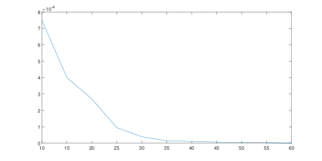
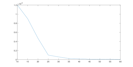
Figure 10: Evaluation at stations $S_{1}$ (top) and $S_{6}$ (bottom) of the empirical norm $L_{k}=\sup_{\overline{x}\in\overline{B},\ \|\overline{x}\|_{\overline{B}}\leq 1}\left\|\overline{\rho}\left(\overline{x}\right)-\displaystyle\sum_{j=1}^{k}\langle\overline{\rho}\left(\overline{x}\right),\overline{\phi}_{n,j}\rangle_{\widetilde{\overline{H}}}\overline{\phi}_{n,j}\right\|_{\overline{B}}$, for values $k=10,15,20,25,30,35,45,60,$ displayed in the horizontal axis.

Figure 11 below displays the mean leave–one out cross validation functional errors

$$E_{c}^{k_{n,m}} = \frac{1}{49}\displaystyle\sum_{h=0}^{48}\left\|\overline{X}_{50}^{c}-\left[\widehat{\overline{X}}_{50}^{c}\right]_{h,k_{n,m}}\right\|_{\overline{B}},\quad c=1,\ldots,6,\quad m=1,2,$$ (33)

at the six pollution stations studied, for the two truncation orders analysed. In the calculation of (33), the Besov and Sobolev norms involved in our function space scenario (31) are computed by projection into Daubechies wavelets of order $N=10$ (see Daubechies92 ), with six resolution levels (see also Figure 1 above).

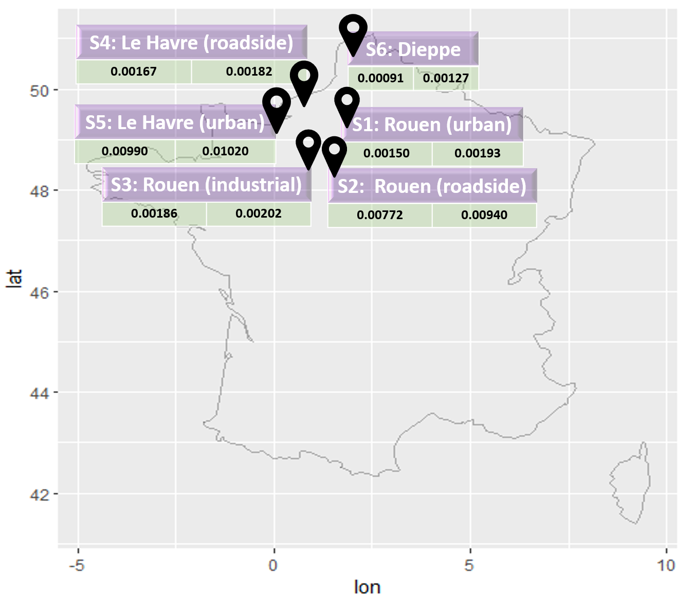
Figure 11: Map displaying mean leave–one out cross validation functional errors (33) at pollution stations $\left\{S_{c},\ c=1,\ldots,6\right\}.$ The truncation parameters $k_{n,1}=\left[\log_{2}\left(\sqrt{n}\right)\right]^{-}$ (on left) and $k_{n,2}=\left[\ln\left(n^{5/2}\right)\right]^{-}$ (on right) have been tested.

In Figure 11, the worst performance is observed at pollution stations $S_{2}$ and $S_{5},$ corresponding to roadside stations. As commented before, the traffic flow is one of the main factors inducing the higher–variability displayed by PM₁₀ concentrations in these stations (see Table 3 in the Appendix). A slightly better performance can be observed with truncation order $k_{n,1},$ but, indeed, a significant improvement cannot be concluded. When larger values of parameter $\beta,$ and hence, of parameter $\gamma,$ defining our function space scenario, are considered, a stronger smoothing of our original data set is achieved, in terms of Sobolev and Besov norms. Thus, a better performance is obtained, with a precision loss, in the approximation of the local behaviour of PM₁₀ concentrations.

6 Final comments

It is well-known that FDA techniques provide a flexible framework for the local analysis of high–dimensional data which are continuous in nature. One of the main subjects in FDA is the suitable choice of the function space, where the observed data take their values. In particular, the norm of the selected space should provide an accurate measure of the local variability of the observed endogenous and exogenous variables, that could be crucial in the posterior representation of the possible interactions with the phenomena of interest and its evolution. That is the case of the real-data example analysed in Section 5.

This paper adopts an abstract Banach space framework, assuming an autoregressive dynamics in time, for all the functional random variables involved in the model. Specifically, an ARBX(1) model is considered. The endogenous and exogenous information affecting the functional response at a given time is incorporated through a suitable linear model, involving a matrix autocorrelation operator. This operator models possible interactions between all endogenous and exogenous functional random variables at any time.

Particularly, the scale of fractional Besov spaces provides a suitable functional framework, where the presented approach can be implemented, modelling local regularity/singularity in an accurate way. Note that the norms in these spaces can be characterised in terms of the wavelet transform. Specifically, wavelet bases provide countable dense systems in Besov spaces, that can be used in the definition of the inner product and associated norms in weighted fractional Sobolev spaces, constructed from the space of square integrable functions on an interval (see Triebel83 , and RuizAlvarez18_JMVA ). Thus, suitable embeddings can be established for applying the construction in Lemma 2.1 in Kuelbs70 . As special cases of well-known Banach spaces within our framework, we refer to $\mathcal{C}([0,1])$ the space of continuous functions on $[0,1],$ with the supremum norm, and $\mathcal{D}([0,1])$ the Skorokhod space of right-continuous functions on the interval $[0,1],$ having a left limit at all $t\in[0,1].$ Note that these spaces have been widely used in the FDA literature in a Banach–valued time series context (see Bosq00 ).

The simulation study and real–data application illustrate the fact that our approach is sufficiently flexible to describing the local behaviour of both, regular and singular functional data. Note that, in the singular case, we can choose a suitable norm that measures the local fluctuations in a precise way. This information is relevant, for example, in the analysis of PM₁₀ concentrations, as was illustrated in Section 5. An individual statistical analysis has been performed in Section 5 at each pollution station. The incorporation of spatial interactions in the analysis could be addressed in a multivariate infinite-dimensional spatial framework, and constitutes the subject of a subsequent paper.

Concerning extending this methodology to a spatiotemporal framework,…

APPENDIX: FIGURES

APPENDIX: TABLES

Table 3: Descriptive statistics from the daily average PM₁₀ concentrations $\mu g~{}m^{-3}$ (the endogenous variable to be predicted) at the six pollution stations selected.

$S_{c}$	Location	Min	Mean	Max	Standard Dev.	% missing
$S_{1}$	Rouen (Urban)	6	19.6	68	7.9	1
$S_{2}$	Rouen (Roadside)	7	24.6	90	9.3	0.4
$S_{3}$	Rouen (Industrial)	4	18.9	80	8.8	1.4
$S_{4}$	Le Havre (Urban)	5	19.2	86	8.5	3
$S_{5}$	Le Havre (Roadside)	8	25.5	86	9.6	1.2
$S_{6}$	Dieppe (Rural)	4	16.3	58	6.3	1.7

Table 4: Descriptive statistics of daily average temperature ($T_{m}$), atmospheric pressure ($PA_{m}$), wind speed ($VV_{m}$) and maximum gradient of temperature ($GT_{max}$) in the three meteorological stations.

$\left(S_{1},~{}S_{2},~{}S_{3}\right)$	$T_{m}$	$VV_{m}$	$PA_{m}$	$GT_{max}$
Min	-6.81	1	974.36	-1.8
Median	10.28	3.8661	1016.71	0.4
Mean	10.11	4.1349	1016.25	1.01
Max	23.95	12	1041.49	14.6
Standard Dev.	6.05	1.65	9.74	2.17

$\left(S_{4},~{}S_{5}\right)$	$T_{m}$	$VV_{m}$	$PA_{m}$	$GT_{max}$
Min	-3.04	1.38	972.88	-1.2
Median	11.1	4.38	1016.59	-0.3
Mean	11.03	5.26	1015.86	0.19
Max	24.08	21.13	1040.9	6.6
Standard Dev.	5.31	2.88	10.07	1.16

$S_{6}$	$T_{m}$	$VV_{m}$	$PA_{m}$	$GT_{max}$
Min	-5.25	1.43	974.13	1.49
Median	10.71	4.38	1016.56	12.32
Mean	10.64	4.85	1015.87	15.44
Max	24.8	14.63	1040.3	72.24
Standard Dev.	5.36	2.13	10.05	9.86

References

• (1) Álvarez-Liébana J, Bosq D, Ruiz-Medina MD (2016) Consistency of the plug-in functional predictor of the Ornstein-Uhlenbeck in Hilbert and Banach spaces. Statist. Probab. Lett. 117:12–22.
• (2) Álvarez-Liébana J, Bosq D, Ruiz-Medina MD (2017) Asymptotic properties of a componentwise ARH(1) plug-in predictor. J. Multivariate Anal. 155:12–34.
• (3) Aneiros-Pérez G, Vieu P (2008) Nonparametric time series prediction: a semi-functional partial linear modeling. J. Multivariate Anal. 99:834–857.
• (4) Angelini C, De Candittis D, Leblanc F (2003) Wavelet regression estimation in nonparametric mixed effect models. J. Multivariate Anal. 85:267–291.
• (5) Antoniadis A, Sapatinas T. (2003) Wavelet methods for continuous-time prediction using Hilbert-valued autoregressive processes. J. Multivariate Anal. 87:133–158.
• (6) Benyelles W, Mourid T (2001) Estimation de la période d’un processus à temps continu à représentation autorégressive. C. R. Acad. Sci. Paris Sér. I Math. 333:245–248.
• (7) Besse PC, Cardot H, Stephenson DB (2000) Autoregressive forecasting of some functional climatic variations. Scand. J. Statist. 27:673–687.
• (8) Blanke D, Bosq D (2016) Detecting and estimating intensity of jumps for discretely observed ARMAD(1,1) processes. J. Multivariate Anal. 146:119–137.
• (9) Bosq D (2000) Linear Processes in Function Spaces. Springer, New York.
• (10) Bueno–Larraz B, Klepsch J (2018) Variable selection for the prediction of $C[0,1]$–valued AR processes using RKHS. arXiv:1710.06660.
• (11) Damon J, Guillas S (2002) The inclusion of exogenous variables in functional autoregressive ozone forecasting. Environmetrics 13:759–774.
• (12) Damon J, Guillas S. (2005) Estimation and simulation of autoregressie Hilbertian processes with exogenous variables. Stat. Inference Stoch. Process. 8:185–204.
• (13) Daubechies I (1992) Ten Lectures on Wavelets. CBMS-NSF Regional Conference Series in Applied Mathematics. Vol. 61, SIAM. Philadelphia.
• (14) Dehling H, Sharipov OS (2005) Estimation of mean and covariance operator for Banach space valued autoregressive processes with dependent innovations. Stat. Inference Stoch. Process. 8:137–149.
• (15) El Hajj L (2011) Limit theorems for $\mathcal{D}([0,1])$-valued autoregressive processes. C. R. Acad. Sci. Paris Sér. I Math. 349:821–825.
• (16) Febrero-Bande M, Galeano P, González-Manteiga W (2008) Outlier detection in functional data by depth measures with application to identify abnormal $NO_{x}$ levels. Environmetrics 19:331–345.
• (17) Fernández de Castro BM, González-Manteiga W, Guillas S (2005) Functional samples and bootstrap for predicting sulfur dioxide levels. Technometrics 47:212–222.
• (18) Ferraty F, Vieu P (2006) Nonparametric Functional Data Analysis: Theory and Practice. Springer, New York.
• (19) Geenens G (2011) Curse of dimensionality and related issues in nonparametric functional regression. Statistics Surveys 5:30–43.
• (20) Goia A, Vieu P (2015) A partitioned single functional index model. Comput. Statist. 30:673–692.
• (21) Goia A, Vieu P (2016) An introduction to recent advances in high/infinite dimensional statistics. J. Multivariate Anal. 146:1–6.
• (22) Gocheva–Ilieva S, Ivanov A, Voynikova D, Boyadzhiev D (2014) Time series analysis and forecasting for air pollution in small urban area: an SARIMA and factor analysis approach. Stoch. Environ. Res. Risk Assess. 28:1045–1060.
• (23) Grivas G, Chaloulakou A (2006) Artificial neural network models for prediction of PM10 hourly concentrations in the greater area of Athens, Greece. Atmospheric Environment 40:1216–1229.
• (24) Guillas S (2002) Doubly stochastic Hilbertian processes. J. Appl. Probab. 39:566–580.
• (25) He H-D, Lu W-Z, Xue Y (2015) Prediction of particulate matters at urban intersection by using multilayer perceptron model based on principal components. Stoch. Environ. Res. Risk Assess. 29:2107–2114.
• (26) Horváth L, Kokoszka P (2012) Inference for Functional Data with Applications. Springer, New York.
• (27) Hsing T, Eubank R (2015) Theoretical Foundations of Functional Data Analysis, with an Introduction to Linear Operators. Wiley, New York.
• (28) Ignaccolo R, Mateu J, Giraldo R (2014) Kriging with external drift for functional data for air quality monitoring. Stoch. Environ. Res. Risk. Assess. 28:1171–1186.
• (29) Kuelbs J (1970) Gaussian measures on a Banach space. J. Funct. Anal. 5:354–367.
• (30) Labbas A and Mourid T (2002) Estimation et prévision d’un processus autorégressif Banach. C. R. Acad. Sci. Paris Sér. I 335:767–772.
• (31) Marion JM, Pumo B (2004) Comparaison des modéles ARH(1) et ARHD(1) sur des données physiologiques. Ann. I.S.U.P. 48:29–38.
• (32) Mas A (2004) Consistance du prédicteur dans le modèle ARH$(1)$: le cas compact. Ann. I.S.U.P. 48:39–48.
• (33) Mas A (2007) Weak-convergence in the functional autoregressive model. J. Multivariate Anal. 98:1231–1261.
• (34) Moritz S (2017) imputeTS: Time Series Missing Value Imputation. http://CRAN.R-project.org/package=imputeTS R package version 2.3.
• (35) Moritz S, Bartz-Beielstein T (2017) imputeTS: Time Series Missing Value Imputation in R. The R Journal 9: 207–218.
• (36) Pang W, Christakos G, Wang J‐F (2009) Comparative spatiotemporal analysis of fine particulate matter pollution. Environmetrics 21:305–317.
• (37) Parvardeh A, Jouzdani NM, Mahmoodi S, Soltani AR (2017) First order autoregressive periodically correlated model in Banach spaces: Existence and central limit theorem. J. Math. Anal. Appl. 449:756–768.
• (38) Paschalidou AK, Karakitsios S, Kleanthous S, Kassomenos PA (2011) Forecasting hourly PM10 concentration in Cyprus through artificial neural networks and multiple regression models: implications to local environmental management. Enviromental Science and Pollution Research 18:316–327.
• (39) Ruiz-Medina MD, Álvarez-Liébana J (2019). A note on strong-consistency of componentwise ARH(1) predictors. Stat. Probab. Lett. 145: 224–248.
• (40) Ruiz-Medina MD, Álvarez-Liébana J (2019) Strongly consistent autoregressive predictors in abstract Banach spaces. J. Multivariate Anal. DOI: 10.1016/j.jmva.2018.08.001.
• (41) Ruiz-Medina MD, Espejo RM (2012) Spatial autoregressive functional plug-in prediction of ocean surface temperature. Stoch. Environ. Res. Risk Assess. 26:335–344.
• (42) Ruiz-Medina MD, Espejo RM, Ugarte MD, Militino AF (2014) Functional time series analysis of spatio–temporal epidemiological data. Stoch. Environ. Res. Risk. Assess. 28:943–954.
• (43) Slini T, Kaprara A, Karatzas K, Mousiopoulos N (2006) PM10 forecasting for Thessaloniki, Greece. Environ. Mod. & Soft. 21:559–565.
• (44) Stadlober E, Hormann S, Pfeiler B (2008) Quality and performance of a PM10 daily forecasting model. Atmospheric Environment 42:1098–1109.
• (45) Triebel T (1983) Theory of Function Spaces II. Birkhauser, Basel.
• (46) Vieu P (2018) On dimension reduction models for functional data. Statist. Prob. Lett. 136:134–138.
• (47) Zhang L, Liu Y, Zhao F (2018) Singular value decomposition analysis of spatial relationships between monthly weather and air pollution index in China. Stoch. Environ. Res. Risk Assess. 32:733–748.
• (48) Zolghadri A, Cazaurang F (2006) Adaptive nonlinear state-space modelling for the prediction of daily mean PM10 concentrations. Environ. Mod. & Software 21:885–894.