Stellar streams from black hole-rich star clusters

Abstract

Nearly a hundred progenitor-less, thin stellar streams have been discovered in the Milky Way, thanks to Gaia and related surveys. Most streams are believed to have formed from star clusters and it was recently proposed that extended star clusters – rich in stellar-mass black holes (BHs) – are efficient in creating streams. To understand the nature of stream progenitors better, we quantify the differences between streams originating from star clusters with and without BHs using direct $N$-body models and a new model for the density profiles of streams based on time-dependent escape rates from clusters. The QSG (Quantifying Stream Growth) model facilitates the rapid exploration of parameter space and provides an analytic framework to understand the impact of different star cluster properties and escape conditions on the structure of streams. Using these models it is found that, compared to streams from BH-free clusters on the same orbit, streams of BH-rich clusters: (1) are approximately five times more massive; (2) have a peak density three times closer to the cluster $1~{}{\rm Gyr}$ post-dissolution (for orbits of Galactocentric radius $\gtrsim 10~{}{\rm kpc}$), and (3) have narrower peaks and more extended wings in their density profile. We discuss other observable stream properties that are affected by the presence of BHs in their progenitor cluster, namely the width of the stream, its radial offset from the orbit, and the properties of the gap at the progenitor’s location. Our results provide a step towards using stellar streams to constrain the BH content of dissolved (globular) star clusters.

1 Introduction

Stellar streams are the debris of dissolved star clusters (for example, Odenkirchen et al., 2001; Grillmair & Dionatos, 2006) and dwarf galaxies (for example, Ibata et al., 1994) and are found in both the inner (Ibata et al., 2019) and outer halo (for example, Belokurov et al., 2006; Newberg et al., 2010; Shipp et al., 2018) of the Milky Way (MW) as well as in other galaxies (for example, Ibata et al., 2001; Martínez-Delgado et al., 2010, 2023). In recent years, there has been a significant uptick in the discovery rate of streams in the MW halo, thanks to the advent of the ESA Gaia space telescope (for example, Malhan et al., 2018; Ibata et al., 2019) and deep, wide-area photometric surveys (for example, Koposov et al., 2014; Bernard et al., 2016; Shipp et al., 2018). Streams are powerful tools in studies of the MW: their shapes provide important constraints on the gravitational potential of the MW (for example, Lynden-Bell & Lynden-Bell, 1995; Koposov et al., 2010, 2023; Küpper et al., 2015; Bovy et al., 2016; Erkal et al., 2019) and their chemistry and orbits help to reconstruct the assembly history of the MW (for example, Bonaca et al., 2021; Li et al., 2022).

The narrow width and low velocity dispersion of the GD-1 stream (Koposov et al., 2010) and the chemistry of its stars (Balbinot et al., 2022) argue for a star cluster origin. However, de Boer, Erkal & Gieles (2020) noted that the initial stellar mass in the GD-1 stream is about five times larger than the estimated maximum mass of a star cluster that can dissolve on that orbit, based on $N$-body calculations of Roche-filling star clusters dissolving in a Galactic tidal field (Baumgardt & Makino, 2003). Curiously, some globular clusters (GCs) with much closer pericentric passages than the GD-1 stream have no noticeable tidal tails associated with them (Kuzma, Da Costa & Mackey, 2018). This suggests that, in addition to the time spent on that orbit, an orbit-independent parameter is required to explain the variation in mass-loss rates of GCs.

Gieles et al. (2021, hereafter G21) showed that the additional parameter is most likely the dynamical effect of stellar-mass black holes (BHs) in the progenitor star cluster. It has been previously shown that $N$-body models of tidally limited star clusters with different initial masses (Pavlík et al., 2018) and densities (G21; Wang et al. 2024) retain a different fraction of BHs and therefore evolve to have different BH populations today (Breen & Heggie, 2013), impacting the mass-loss of the cluster (Banerjee & Kroupa, 2011; Giersz et al., 2019). G21 build upon this to show that the tidal tails associated with the halo GC Palomar 5 (hereafter Pal 5) – just like the GD-1 stream – also contain more mass than can be explained by the models of cluster dissolution of Baumgardt & Makino (2003). Because this is the most prominent stream with a known progenitor, G21 attempted to reproduce the observed properties of both the cluster and the stream with $N$-body simulations. They found that both the peculiar large half-light radius of $r_{\rm eff}\simeq 20\,{\rm pc}$ for Pal 5 as well as the mass in the tails can only be reproduced if the cluster contains a BH population, constituting a fraction of $f_{\rm BH}\simeq 0.2$ of the total present-day cluster mass. From these models, G21 found that both the mass in the tails as well as $r_{\rm eff}$ correlate with $f_{\rm BH}$ and concluded that BH-rich GCs are the likely progenitors of cold streams. The higher mass-loss rate of GCs with BHs also helps to explain the shape of the GC mass function and the distribution of nitrogen-rich stars in the inner halo that are believed to originate from GCs (Gieles & Gnedin, 2023, hereafter GG23).

In addition to GD-1 and the Pal 5 stream, there are more streams with masses above the maximum masses of clusters that can dissolve on their orbits. Figure 1 displays the masses of the streams included in Patrick, Koposov & Walker (2022) that are believed to have had GC progenitors which have now dissolved as a function of the Galactocentric radius of their equivalent circular orbits with the same average mass-loss rate ($R_{\rm eff}=R_{\rm p}(1+e)$, where $R_{\rm p}$ is the Galactocentric radius at pericentre and $e$ is the orbital eccentricity, Baumgardt & Makino 2003). In addition we include Jet, C-19, and Phlegethon streams which are believed to have GC progenitors. The orbital parameters used to calculate $R_{\rm eff}$ for the streams in Patrick et al. (2022) were obtained from Li et al. (2022) for all streams except GD-1 and Pal 5 which used the values from Bonaca et al. (2020) and Küpper et al. (2015), respectively. The mass estimates and orbital parameters for Jet, C-19, and Phlegethon were taken from Ferguson et al. (2022), Martin et al. (2022), and Ibata et al. (2018) respectively. The lines show model predictions (GG23) for the initial mass, after stellar evolution, of GCs with a dissolution time of $10~{}{\rm Gyr}$ without BHs (blue) and with BHs (orange). The expression for the disruption time of GG23 (their equation 6) has two parameters, $y$ relates the mass-loss rate to the cluster mass and $\dot{M}_{\rm ref}$ is the mass-loss rate at fixed reference mass ($2\times 10^{5}~{}{\rm M}_{\odot}$). For the three cases shown these are $(y,\dot{M}_{\rm ref})=(2/3,-30\,{\rm M}_{\odot}/{\rm Myr})$ for ‘noBH’ (approximately the Baumgardt & Makino 2003 results), $(4/3,-45\,{\rm M}_{\odot}/{\rm Myr})$ for ‘wBH median’ (used in their GC population models) and $(2,-95\,{\rm M}_{\odot}/{\rm Myr})$ for ‘wBH max’ which corresponds to their lowest density $N$-body models where the effect of BHs on the mass-loss rate was maximal.

Apart from Ophiuchus and Phlegethon, which lie well below the noBH line, and Phoenix which lies just below the noBH line, every other stream’s mass exceeds the noBH limit. Patrick et al. (2022) calculate the mass of the stream by generating a new simulated stellar population from the fitted colour-magnitude diagram, allowing the mass estimate to account for unobserved low mass stars. Yet, these masses are likely incomplete because Patrick et al. (2022) did not include features offset from the stream track (such as the spur of GD-1), nor corrections for stars outside of their defined ends of the streams which are difficult to pick out from the background. This implies that their mass estimates are lower limits of the initial stellar mass of the streams’ progenitor GCs. A particularly stark example is that of GD-1, for which Patrick et al. (2022) determine the stream mass to be $\sim 5\times 10^{3}\,{\rm M}_{\odot}$, whereas de Boer et al. (2020) estimate a total mass of $\sim 10^{4}~{}{\rm M}_{\odot}$ (after stellar evolution mass loss) by comparison of the observed stream with a mock population of stars generated through isochrone fitting and convolved with observational effects. In addition, it is important to note that the mass estimate of C-19 in Martin et al. (2022) is a lower limit as it is expected that the stream extends beyond the observed range. This comparison confirms that most streams dissolved faster than what is expected from models of GCs without BHs, calling for stream formation models that include the effect of BHs.

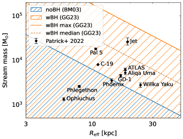
Figure 1: The mass of the streams from Patrick et al. (2022), that are believed to have had GC progenitors which have now dissolved, as a function of the Galactocentric radius of the equivalent circular orbit with the same average mass-loss rate, $R_{\rm eff}$, (Baumgardt & Makino, 2003). In addition, we include Jet (Ferguson et al., 2022), C-19 (Martin et al., 2022), and Phlegethon (Ibata et al., 2018) (denoted by the diamond markers) which are also believed to have GC progenitors. The blue hatched region denotes the area of parameter space that can be populated by GCs without BHs that can dissolve within $10~{}{\rm Gyr}$ (Baumgardt & Makino, 2003). The orange hatched region denotes the area of parameter space that can be populated by GCs with BHs that can dissolve within $10~{}{\rm Gyr}$ and the dashed (solid) orange line marks the median (maximum) mass of a GC with BHs and a dissolution time of $10~{}{\rm Gyr}$ (see text for details). The error bars do not take into account the possibility of unobserved low density extensions to the streams and therefore these data points should be regarded as lower bounds on the progenitor mass.

Most stream modelling efforts to date have focused on the shape and features such as epicyclic overdensities (for example, Sanders, 2014; Bovy, 2014; Fardal et al., 2015; Küpper et al., 2015) and could therefore adopt a constant escape rate. However, it is well understood that the mass-loss rate is not constant, instead the magnitude of the mass-loss rate decreases approaching dissolution for noBH GCs (Fukushige & Heggie, 2000; Baumgardt, 2001; Baumgardt & Makino, 2003; Lamers et al., 2010), while it increases for wBH GCs (Banerjee & Kroupa 2011; Giersz et al. 2019; G21), and there is yet to be a study of the dependence of a stream’s morphology on the progenitor’s mass-loss rate. Motivated by this, the suggestions that BH-rich clusters are the progenitors of (most of the) cold stellar streams (G21) and that wBH streams should exhibit a gap at the progenitor’s position post-dissolution (de Boer et al., 2020), and also by the availability of more luminosity-based mass estimates and corresponding density profiles of streams (for example, de Boer et al. 2020; Patrick et al. 2022), we here present a model for streams based on a time-dependent mass-loss history of their progenitor clusters. To parameterise this new model, we use direct $N$-body simulations of star clusters dissolving in a Galactic tidal field with and without BHs, to shed light on the nature of stream progenitors by investigating whether the structure of a stream can be used to discriminate between BH-rich and BH-free progenitors and identify features which display a dependence on the retained BH population.

This paper is organised as follows: in Section 2 we introduce the $N$-body simulations and the model for the density profiles of streams with time-dependent mass-loss history. In Section 3 we discuss the impact of a BH population in the progenitor cluster on stream properties and the discussion and conclusions are presented in Section 4 and Section 5, respectively.

2 A model for streams from time-dependent mass-loss rates

In this section we present a model for streams forming from clusters on circular orbits with time-dependent mass-loss rates. We first present two $N$-body models of clusters with and without BHs in Section 2.1 and then describe the (semi-)analytic model for the stream density profile in Sections 2.2–2.4. In Section 2.5 we compare the stream model to the $N$-body simulations.

2.1 $N$-body simulations

To quantify the effect of a BH population on the resulting stream, we run $N$-body models of two clusters on the same orbit, where one model contains BHs (‘wBH-Nbody’) and the other cluster does not (‘noBH-Nbody’). We run both simulations with PeTar (Wang et al., 2020), which includes the effect of stellar and binary evolution (Hurley et al., 2000, 2002) with the recent updates for massive star winds and BH masses from Banerjee et al. (2020). We adopt the rapid supernova mechanism by Fryer et al. (2012), for which $60\%$ ($70\%$) by number (mass) of the BHs do not receive a natal kick due to fall back, for the adopted stellar initial mass function (IMF) (Kroupa, 2001, in the range $0.1-100\,{\rm M}_{\odot}$) and metallicity ($Z=10^{-3}$, i.e. ${\rm[Fe/H]}\simeq-1.1$). For the noBH-Nbody model we prevent the formation of BHs by truncating the IMF at $20~{}{\rm M}_{\odot}$. We adopt a ‘GD-1 like’ orbit: a circular orbit at a Galactocentric radius of $R=20\,$kpc in a singular isothermal sphere (SIS) using the Galpy library (Bovy, 2015).

The initial positions and velocities of the stars are drawn from a Plummer model (Plummer, 1911) truncated at 20 times the half-mass radius ($r_{\rm h}$). We define the initial $r_{\rm h}$, $r_{\rm h,0}$, in units of the half-mass radius of a Roche-filling cluster ($r_{\rm h,f}$), for which we adopt the value from Hénon (1961) of $r_{\rm h,f}=0.15r_{\rm J}$, where $r_{\rm J}$ is the Jacobi radius. For the SIS, $r_{\rm J,0}=\left[GM_{0}/(2\Omega^{2})\right]^{1/3}$, where $M_{0}$ is the initial mass of the cluster and $\Omega=V_{\rm c}/R$ is the angular frequency of the orbit. Because clusters expand as a result of stellar mass loss, we start with $r_{\rm h,0}<r_{\rm h,f}$. For the noBH-Nbody cluster we adopt $r_{\rm h,0}=0.7r_{\rm h,f}$ and for the wBH-Nbody cluster we adopt a slightly smaller radius of $r_{\rm h,0}=0.6r_{\rm h,f}$ because this cluster expands more due to the dynamical effect of the BHs following stellar mass loss. What remains to be decided is the initial number of stars ($N$) of both models. We find values for $N$ by iteration, such that both models dissolve approximately at an age of 8 Gyr. Our initial estimates are guided by the analytic expressions for $\dot{M}$ and $M(t)$ of GG23 for clusters with different BH contents. After a few iterations of $N$-body models with different $N$ we settled on $N=4600$ for the noBH-Nbody model and $N=28500$ for the wBH-Nbody model, where the difference is due to the higher mass loss rate of a GC with BHs. The evolution of the total cluster mass, the mass-loss rate and the mass of the BH population of both models is shown in Fig. 2. In the next subsection we discuss the resulting streams as well as a generative model for the stream that we base on the mass evolution of these $N$-body models.

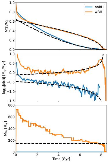
Figure 2: The evolution of the total cluster mass (top), its mass-loss rate (middle), and the mass of the black hole population (bottom) of the two $N$-body models discussed in Section 2.1 (noBH-Nbody in blue and wBH-Nbody in orange). The over-plotted black dashed lines are $M(t)$ (equation 2) and $\dot{M}(t)$ (equation 3), with $t_{\rm d}=8.2\,$Gyr and $\eta=0.4;M_{\rm i}=1.66\times 10^{3}\,{\rm M}_{\odot}$ (noBH) and $\eta=-0.8;M_{\rm i}=1.12\times 10^{4}\,{\rm M}_{\odot}$ (wBH). The slight under-prediction of $M(t)$ in the first half of the evolution of the noBH case is because our model does not include stellar evolution mass-loss (see text for details). In the bottom panel the over-plotted dashed line corresponds to $M_{\rm BH}=150~{}{\rm M}_{\odot}$, the value used in our models.

2.2 Mass-loss rate

In this section we develop a semi-analytic model for the streams from clusters with and without BHs and benchmark the results against the $N$-body models from Section 2.1.

We only model the mass-loss rate as the result of stellar escape through the Lagrange points, that is, we do not include mass-loss by stellar evolution, which dominates in the early evolution of the noBH model until the mass-loss due to dissolution exceeds the mass-loss due to stellar evolution (which occurs at $\sim 0.5~{}{\rm Gyr}$ for noBH-Nbody). After that, the mass-loss rate is well described by a power-law dependence on $M$ of the form

$$\dot{M}=-AM^{\eta}=-\frac{M_{\rm i}}{(1-\eta)t_{\rm d}}\left(\frac{M}{M_{\rm i}}\right)^{\eta},$$ (1)

where $M$ is the cluster mass and $M_{\rm i}<M_{0}$ is the remaining mass after most stellar evolution mass loss has occurred. From this we can obtain the GC mass and mass-loss rate as a function of time since disruption of the GC begins,

$$M(t)=M_{\rm i}\left(1-\frac{t}{t_{\rm d}}\right)^{1/(1-\eta)},$$ (2)

and therefore when combined with equation (1), we get

$$\dot{M}(t)=-\frac{M_{\rm i}}{(1-\eta)t_{\rm d}}\left(1-\frac{t}{t_{\rm d}}\right)^{{\eta}/({1-\eta})}.$$ (3)

The mass dependence of $\dot{M}$ is encapsulated in the parameter $\eta$, where the mass evolution of noBH clusters is well described by $\eta\simeq 1/3$ (Baumgardt & Makino, 2003) and for wBH clusters, $-1\lesssim\eta\lesssim-1/3$ (GG23). The above expressions are simplified versions of $M(t)$ and $\dot{M}(t)$ expressions recently presented in GG23. These authors showed with $N$-body models that clusters with lower initial densities retain more of their BHs, and have a smaller (i.e. more negative) $\eta$. For $\eta<0$, the (absolute) mass loss rate increases towards dissolution, which is the result of the increasing fraction of mass in BHs. GG23 also shows that the constant of proportionality $A$ (which is inversely proportional to $t_{\rm d}$) in equation (1) depends on $\eta$, $M_{0}$ and the strength of the tidal field.

The dependence of $\eta$ on the mass of the black hole population, $M_{\rm BH}$, is because there exists a critical $f_{\rm BH}$ for tidally limited GCs on order of a few percent at which the stellar mass-loss rate equals the BH mass-loss rate and therefore $f_{\rm BH}$ remains constant (Breen & Heggie, 2013). If $f_{\rm BH}>f_{\rm BH,\,crit}$ then $f_{\rm BH}$ increases which leads to an accelerating mass-loss rate (i.e.$~{}\eta<0$) and a BH dominated cluster (Banerjee & Kroupa 2011; Giersz et al. 2019; G21). On the other hand, if $f_{\rm BH}<f_{\rm BH,\,crit}$ then $f_{\rm BH}$ decreases leading to a decelerating mass-loss rate (i.e.$~{}\eta>0$) (Fukushige & Heggie, 2000; Baumgardt, 2001; Baumgardt & Makino, 2003; Lamers et al., 2010). It is important to note that a noBH GC with a low initial density can have a similar high mass-loss rate as a wBH GC, but G21 show this area of parameter space is extremely small and as such we consider an accelerating mass-loss rate to be the result of a retained stellar-mass BH population.

Rather than using the full expressions from GG23, we here stick to the simpler expressions from above and find the values of $M_{\rm i}$ and $\eta$ that are needed to describe the two $N$-body models. The mass and mass-loss history for the $N$-body models and the analytic approximations are displayed in the top two panels of Fig. 2. We find $M_{\rm i}$ from the total stellar mass in the $N$-body model post-dissolution such that mass lost due to stellar evolution is not included. For the noBH model we then find $M_{\rm i}\simeq 0.64M_{0}\simeq 1.66\times 10^{3}~{}{\rm M}_{\odot}$ and by varying $\eta$ we find that $\eta\simeq 0.4$ provides a good description of the evolution of $M(t)$. A similar mass dependence of the mass-loss rate was found previously in models of clusters without BHs (Lamers, Baumgardt & Gieles, 2010). For the wBH model we find $M_{\rm i}\simeq 0.62M_{0}\simeq 1.12\times 10^{4}\,{\rm M}_{\odot}$ and $\eta\simeq-0.8$. This negative $\eta$ causes mass loss to accelerate towards dissolution, as found here (see orange lines in top and middle panels of Fig. 2) and also in other models of dissolving clusters with BHs (Giersz et al. 2019; Wang 2020; GG23).

We plot the resulting analytic expressions for $M(t)$ and $\dot{M}(t)$ in Fig. 2. The $M(t)$ result for the noBH model slightly under-predicts the $N$-body models in the first $\sim 4\,$Gyr (top panel of Fig. 2), which is because in that period the stellar evolution mass-loss rate is of comparable magnitude to the mass-loss rate from escape. These expressions ensure that a GC will dissolve at a chosen dissolution time (informed by $N$-body simulations), which is key when examining the growth of the gap that forms at the progenitor’s position post-dissolution.

2.3 The Quantifying Stream Growth (QSG) model

To investigate the differences in streams resulting from the noBH and wBH clusters, a model of the growth of streams is required. Here we introduce a new model that follows the formalism of Erkal & Belokurov (2015). It adopts a reference frame that is centred on the cluster and co-rotates with the orbit, where the $x$-axis points towards the galactic anti-centre, the $y$-axis points along the orbit, and the $z$-axis is along the angular momentum vector of the orbit, perpendicular to the orbital plane. We restrict ourselves to a cluster on a circular orbit, with galactocentric radius $R$ and circular velocity $V_{\rm c}$, within a spherical potential. Stars are then assumed to escape through the Lagrange points, offset from the centre of the cluster along $x$ by a distance $\pm f_{\rm e}\,r_{\rm J}(M(t))$, where $f_{\rm e}$ is a dimensionless constant of order unity to be determined, and they are released with some initial velocity offset $\vec{\Delta v}=(\Delta v_{x},\Delta v_{y},\Delta v_{z})$. In this model the velocity offset in the $y$-direction ($\Delta v_{y}$) is related to the escape radius by $\epsilon$, a dimensionless free parameter of order unity, such that $\Delta v_{y}$ is the random component of the velocity (in the galactocentric reference frame $\epsilon=1$ means that escapers have on average the progenitors angular velocity, whereas $\epsilon=0$ corresponds to escapers having on average the progenitors orbital velocity). The equations of motion for stars that have escaped the progenitor are derived in Appendix A and it is important to note that these equations ignore the progenitor’s mass as they are intended to describe the stripped stars’ motion when the cluster potential experienced by the escapers is negligible compared to the galactic potential. The time-dependent angle from the centre of the potential of the ejected particle (relative to the progenitor) is given by

$$\begin{array}[]{ll}\phi_{1}(t)=&-\frac{4-\gamma^{2}}{\gamma^{2}}\left(\Delta v_{y}+(1+\epsilon)\frac{f_{\rm e}r_{\rm J}}{R}V_{\rm c}\right)\frac{t}{R}\\ &-\frac{2}{\gamma^{3}}(\gamma^{2}-2-2\epsilon)\frac{f_{\rm e}r_{\rm J}}{R}\sin\left(\gamma\Omega t\right)\\ &+\frac{1}{\gamma^{3}}\frac{4\Delta v_{y}}{V_{\rm c}}\sin\left(\gamma\Omega t\right)\\ &-\frac{1}{\gamma^{2}}\frac{2\Delta v_{x}}{V_{\rm c}}\left(1-\cos\left(\gamma\Omega t\right)\right),\end{array}$$ (4)

where

$$\gamma^{2}=3+\frac{R^{2}}{V_{\rm c}^{2}}\partial_{R}^{2}\Phi(R),$$ (5)

is the ratio of epicyclic frequency to the angular frequency, $\Phi(R)$ is the spherical galactic potential, $t$ is the time since escape, and the negative sign in front of the equation means that stars ejected from the outer (inner) Lagrange point fall behind (move ahead) of the progenitor, as expected.

The radial offset (that is, the displacement from the progenitor’s orbital track in the direction of the galactic anti-centre) as a function of time is given by

$$\begin{array}[]{ll}\displaystyle\Delta r(t)=&f_{\rm e}r_{\rm J}\cos(\gamma\Omega t)+\frac{2R}{\gamma^{2}}\left(\frac{\Delta v_{y}}{V_{\rm c}}+(1+\epsilon)\frac{f_{\rm e}r_{\rm J}}{R}\right)\times\\ &\left(1-\cos(\gamma\Omega t)\right)+\frac{R\Delta v_{x}}{V_{\rm c}}\frac{\sin(\gamma\Omega t)}{\gamma},\end{array}$$ (6)

where we note that $\Delta r(t=0)=\Delta x(t=0)$. The velocity in the $z$ direction simply tilts the orbital plane of the escaping star (Erkal, Sanders & Belokurov, 2016) and the resulting motion perpendicular to the progenitor’s orbital plane is given by

$$\Delta z(t)=\Delta v_{z}\frac{R}{V_{\rm c}}\sin{\left(\frac{V_{\rm c}}{R}t\right)}.$$ (7)

The density at a point along the stream is the product of the mass-loss rate and the $\phi_{1}$ distribution of that mass integrated from the start of stripping up until the observation time. This can be expressed in terms of the velocity distribution and used to map the density along the stream, $\rho(\phi_{1},t)$, at all times

$$\rho(\phi_{1},t)=\frac{\gamma^{2}}{4-\gamma^{2}}\int_{0}^{t}\!\frac{R}{t-t^{\prime}}\,|\dot{M}(t^{\prime})|\,P(\Delta v_{y})\,{\rm d}t^{\prime},$$ (8)

where $P(\Delta v_{y})$ is the probability density function of $\Delta v_{y}$. This equation sums up all possible stripping events up to the observation time and scales their contribution by the velocity distribution. By assuming a Gaussian distribution of offset velocities, the probability of a particular value is

$$\displaystyle P(\Delta v_{y})=\frac{1}{\sqrt{2\pi\sigma^{2}}}\,e^{-\frac{1}{2}\left(\frac{\Delta v_{y}}{\sigma}\right)^{2}},$$ (9)

where $\sigma$ is the velocity dispersion of a Plummer model (Plummer, 1911) at the escape radius,

$$\sigma=\sqrt{\frac{GM}{6a}}\left[1+\left(\frac{f_{\rm e}r_{\rm J}}{a}\right)^{2}\right]^{-1/4}.$$ (10)

To get the ratio $f_{\rm e}r_{\rm J}/a$ we assume that the cluster fills the Roche radius, that is, $r_{\rm h}/r_{\rm J}\simeq 0.15$ (Hénon, 1961) and we note that $a\simeq 1.305\,r_{\rm h}$ for Plummer’s model. A time-dependent expression for $\Delta v_{y}$ is found by ignoring the oscillatory terms in equation (4) to obtain the average motion of a star

$$\phi_{1}(t)=-\frac{4-\gamma^{2}}{\gamma^{2}}\left(\Delta v_{y}+(1+\epsilon)\frac{f_{\rm e}r_{\rm J}}{R}V_{\rm c}\right)\frac{t}{R},$$ (11)

and rearranging for $\Delta v_{y}$

$$\Delta v_{y}=-\frac{\gamma^{2}}{4-\gamma^{2}}\frac{\phi_{1}R}{t}+(1+\epsilon)\frac{f_{\rm e}r_{\rm J}}{R}V_{\rm c}.$$ (12)

By switching variables to $\tau=(t-t^{\prime})^{-1}$ an expression that can be easily numerically evaluated is obtained,

$$\rho(\phi_{1},t)=\frac{\gamma^{2}}{4-\gamma^{2}}\int_{\tau_{i}}^{\tau_{f}}\frac{R}{\tau}\,|\dot{M}(\tau)|\,P(\Delta v_{y})\,{\rm d}\tau.$$ (13)

Equation (13) can then be evaluated at regular intervals of $\phi_{1}$ at any point in time, before or after dissolution, to gain the 1-D density profile of the resulting stream. Hereafter, this (semi-)analytic model to quantify the stream growth is referred to as the QSG-AN (Quantifying Stream Growth - ANalytic) model. The model has two dimensionless parameters, $\epsilon$ and $f_{\rm e}$, that we will determine through a comparison to the $N$-body models in Section 2.5. $\epsilon$ and $f_{\rm e}$ relate the mean velocity of escapers to the escape radius and set the escape radius respectively. From this, and equation (11), it is clear that there is some degeneracy between them as both affect the mean drift velocity of escapers (i.e. the location of the centre of the $\Delta v_{y}$ distribution). However, $f_{\rm e}$ is the sole free parameter dictating the velocity dispersion in addition to the cluster mass. Throughout this work we use the analytic mass-loss rate from Section 2.2 as this gives us the smoothed case for a cluster with the given initial conditions removing the stochastic noise of dynamical ejections. However, one could also use the mass loss rate from numerical $N$-body simulations so long as it is corrected for the mass-loss due to stellar evolution.

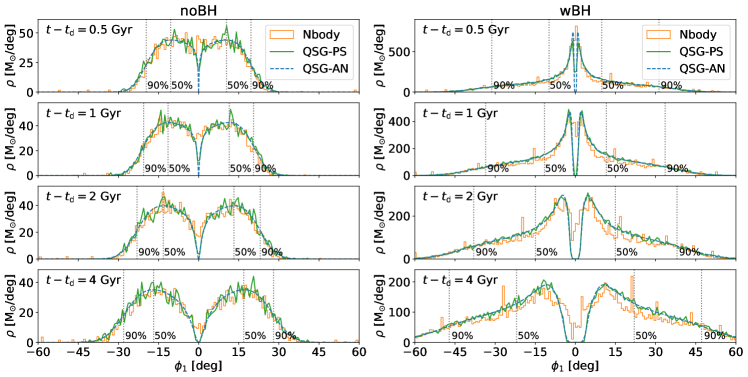
Figure 3: A comparison of the QSG-PS (green solid) and QSG-AN (blue dashed) models with the $N$-body simulations (orange) for the noBH model (left) and wBH model (right) at four times. From top to bottom these times are $0.5$, $1$, $2$, and $4~{}{\rm Gyr}$ after dissolution. The vertical dashed lines denote the $50^{\rm th}$ and $90^{\rm th}$ percentile by mass. Due to the differing $M_{\rm i}$ and $\eta$, $0.5~{}{\rm Gyr}$ post-dissolution (top row) the peak linear density is over an order of magnitude greater in the wBH model than in the noBH model and remains a factor of $\sim 5$ greater $4~{}{\rm Gyr}$ post-dissolution (bottom row). It is also seen that the $90^{\rm th}$ percentile is over twice the $50^{\rm th}$ percentile for the wBH model, whereas it is less than twice the $50^{\rm th}$ percentile in the noBH model.

2.4 Particle spray method

QSG-AN does not capture all elements of a stream’s structure, not only because it does not include the epicyclic over-densities due to the use of equation (11) which ignores the oscillatory terms, but because it only describes the one-dimensional density profile and therefore offers no insight in the stream offset from the orbit, nor the width. To describe these additional features of a stream we employ a Monte Carlo model using equations (4), (6), and (7) for motion along the stream, radially to the stream and perpendicular to the progenitor’s orbital plane respectively, we refer to the resulting particle spray model as QSG-PS (Quantifying Stream Growth - Particle Spray). In QSG-PS a population of stars is generated, their escape times are calculated from equation (3) and their $f_{\rm e}r_{\rm J}$ are calculated from the mass in the cluster at their escape times (equation 2). Their velocity offset in each direction ($\Delta v_{x}$, $\Delta v_{y}$, $\Delta v_{z}$) is sampled from a Gaussian distribution centered on zero with a width equal to the velocity dispersion given by equation (10). Then, at any point in time prior- or post- dissolution those stars that have escaped the cluster can be selected and their positions calculated from equations (4), (6), and (7).

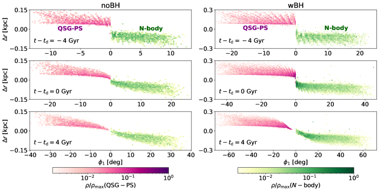
Figure 4: A comparison of QSG-PS (Red-Purple) with the $N$-body simulations (Yellow-Green) for the noBH models (left) and wBH models (right) for stream projections on the orbital plane. The density normalization, $\rho_{\rm max}$, is the maximum density across all the snapshots for both wBH and noBH models, hence why the noBH models never reach the maximum value. The leading and trailing tails are symmetric, such that no information is lost by showing one tail of each model, which we do here for ease of comparison.

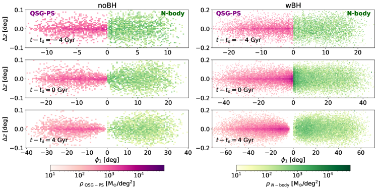
Figure 5: A comparison of QSG-PS (Red-Purple) with the $N$-body simulations (Yellow-Green) for the noBH models (left) and wBH models (right) for stream projections on the $\phi_{1}-z$ plane (that is as seen from the centre of the galaxy). As in Fig. 4, the density normalization, $\rho_{\rm max}$, is the maximum density across all the snapshots for both wBH and noBH models and the leading and trailing tails are symmetric, such that no information is lost by showing one tail of each model.

2.5 Comparison to $N$-body

To compare to the $N$-body models of Section 2.1, we adopt an SIS potential for the galaxy with $V_{\rm c}=220~{}{\rm km/s}$ as in the $N$-body models. We create stream models without BHs and with BHs using QSG-AN(QSG-PS), which we refer to as noBH-QSG-AN(noBH-QSG-PS) and wBH-QSG-AN(wBH-QSG-PS), respectively. The models use the values for $M_{\rm i}$ and $\eta$ and the analytic expressions for $M(t)$ and $\dot{M}(t)$ provided in Section 2.2 (shown also as black dashed lines in Fig. 2). For all models we adopt circular orbits at $R=20~{}{\rm kpc}$ about the SIS potential and $t_{\rm d}=8.2~{}{\rm Gyr}$. In the QSG-PS model, $0.4~{}{\rm M}_{\odot}$ stars are used such that noBH-QSG-PS has $N=4150$, which is less than in the $N$-body stream due to the differing initial mass because we do not include stellar evolution mass loss (see Section 2.2). The wBH-QSG-PS model has $N=2.8\times 10^{4}$, similar to the $N$-body simulations and we approximate the mass in the BH population as a constant, $M_{\rm BH}=150~{}{\rm M}_{\odot}$, which is a reasonable approximation for $M_{\rm BH}(t)$ in the $N$-body simulation for the $3~{}{\rm Gyr}$ leading up to dissolution in which a significant fraction of the stream forms.

We find the values for the two model parameters $\epsilon$ and $f_{\rm e}$ by comparing the distribution of stars in the $\phi_{1}$ and $\Delta r$ directions in the QSG-PS models and the density profile of the QSG-AN models to those of the $N$-body models. The resulting QSG-AN density profiles and QSG-PS streams are in very good agreement with the $N$-body simulations for $\epsilon\simeq 0.57$ and $f_{\rm e}\simeq 1.5$, as can be seen in Fig. 3 (QSG-AN) and Figs. 4 & 5 (QSG-PS). It is these values that are used throughout the rest of this work in both QSG-AN and QSG-PS and in both wBH and noBH cases. We stress that this is an effective model and as such one should not read too much into the meaning of $\epsilon$. Instead $\epsilon$ should be regarded as a parameter that can be obtained from $N$-body models. However, for completeness, we note that $\epsilon<1$ does indicate prograde in an inertial frame (retrograde in a co-rotating frame).

As seen in Fig. 3, both QSG-AN and QSG-PS are both able to reproduce accurate linear density profiles for streams with and without BHs. However, the density profile does deviate somewhat post-dissolution within the gap. This is due to the idealised nature of our model assuming that even the final stars follow our prescription for the escape conditions. Despite this, they capture important features such as the peak of the density profile, size and shape of the wings, and the size of the gap remarkably well for such a simple model.

As is seen in Fig. 4, QSG-PS is able to reproduce the structure of the stream in the $\phi_{1}$-$\Delta r$ plane well in both wBH and noBH cases and both prior and post-dissolution. In particular, it captures the length, width, offset from the progenitor’s orbital track, and mass distribution along the stream well. However, due to the simplifying assumptions and the idealised nature of the escape conditions there are some aspects where it diverges. In particular, because we assume a constant $M_{\rm BH}$ in the wBH-QSG-PS model there are fewer stars within the gap than in the wBH-Nbody model. In addition, just before dissolution we still assume that the stars follow our prescription for the escape conditions which may not be true and this manifests as the stream being very narrow near the progenitor’s position post-dissolution, whereas the $N$-body models have a greater spread in $\Delta r$ near to the progenitor. This disparity is particularly noticeable in the wBH, 4Gyr (bottom, right) panel of Fig. 4. We see that this disparity between QSG-PS and $N$-body models is greatly reduced in the noBH models (see the bottom, left panel of Fig. 4), implying the need for a study of the escape conditions of stars in wBH GCs as they approach dissolution.

As seen in Fig. 5, QSG-PS does not fair as well in the $\phi_{1}$-$\Delta z$ plane. The simplistic nature of the QSG-PS model does not reproduce the diffuse nature of the stream in the $\phi_{1}\,-\,\Delta z$ plane. Instead, QSG-PS produces a much sharper over-density at the orbital plane, $\Delta z=0$, which resembles a combination of a narrow and broad Gaussian. This is seen in other particle spray codes as well, e.g. Gibbons et al. (2014).

The simple, fast, flexible nature of the QSG models makes them invaluable tools to explore the impact of the progenitor’s properties on the structure of the resulting stream. With further refinement of the prescription of escape conditions to produce even more realistic streams, the QSG models have a wide range of application including constraining the possible parameter space of stream progenitors. In the next section we discuss the properties of the wBH and noBH streams in detail.

3 The Impact of a Retained Black Hole Population

From the models discussed in the previous section, we find that there are four main aspects of the stream’s structure that differ due to the retained BH population: (1) The mass in the stream / inferred mass-loss rate; (2) the growth rate / stream length; (3) the shape of the central gap after dissolution (which primarily depends on the mass-loss rate) and (4) the width and offset of the stream near the progenitor in the radial direction from the progenitor’s orbital track soon after dissolution. The first three are because of differences in the mass-loss rate and the fourth property is sensitive to the retained mass of the BH population. Below we discuss all four properties guided by the results from the models from the previous section.

3.1 Mass in the stream

Here we discuss the mass in the stream at different moments after dissolution. Figure 6 displays the cumulative mass in the stream as a function of angular displacement from the progenitor’s position for the noBH-Nbody and wBH-Nbody models at four times since dissolution ($t-t_{\rm d}=0,1,2,4~{}{\rm Gyr}$). These are compared to the initial mass of the noBH-Nbody model after stellar evolution ($M_{\rm i}=1.66\times 10^{3}~{}{\rm M}_{\odot}$). It is observed, as expected, that for all times since dissolution the cumulative mass of the noBH-Nbody model tends to $M_{\rm i}$, whereas the wBH-Nbody model significantly exceeds $M_{\rm i}$ even at small $\phi_{1}$. Since the gap grows after dissolution in both models, the enclosed mass at some distance of the wBH-Nbody model will eventually drop below $M_{\rm i}$ of the noBH-Nbody model. Because the time since dissolution is unknown, this could potentially lead to misclassifying a wBH stream as a noBH stream. However, even at $t-t_{\rm d}=4~{}{\rm Gyr}$ the mass within $10\degree$ of the progenitor of the wBH-Nbody model exceeds the theoretical maximum for a BH-free GC on this orbit; this is owed not only to the greater initial mass of the wBH-Nbody model, but to the accelerating mass-loss rate resulting in the same fraction of the mass being concentrated closer to the progenitor’s position as seen in Fig. 3.

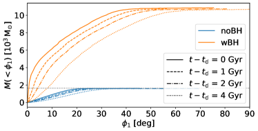
Figure 6: The cumulative mass as a function of the angular displacement from the progenitor along the stream for the noBH-Nbody (blue) and wBH-Nbody (orange) models at four times since dissolution (shown by the different linestyles). The over-plotted grey dotted line is at $M_{\rm i}=1.66\times 10^{3}~{}{\rm M}_{\odot}$.

It is not just the total mass in the stream that differs but, as seen in Fig. 3, the distribution of this mass differs as well. In the noBH-Nbody model the $\phi_{1}$ coordinate of the $90^{\rm th}$ percentile by mass is less than twice that of the $50^{\rm th}$ percentile, whereas in the wBH-Nbody model the $\phi_{1}$ coordinate of the $90^{\rm th}$ percentile is over twice that of the $50^{\rm th}$ percentile. In addition, the work of GG23 allows us to estimate the maximum expected density of a stream from a noBH progenitor on the same orbit with the same dissolution time ($t_{\rm d}=8.2~{}{\rm Gyr}$) from $\rho\propto\dot{M}/\overline{v}$. Taking the initial mass from section 2.2 ($M_{\rm i}=1.66\times 10^{3}~{}{\rm M}_{\odot}$) and the maximum mass-loss rate of this cluster on this orbit ($\dot{M}\simeq-0.3~{}{\rm M}_{\odot}/{\rm Myr}$, from equation 1 of GG23), we then need the mean drift velocity of a typical star, $\overline{v}$. This is found by differentiating equation (11) with respect to time

$$\dot{\phi}_{1}R=-\frac{4-\gamma^{2}}{\gamma^{2}}\left(\Delta v_{y}+(1+\epsilon)\frac{f_{\rm e}r_{\rm J}}{R}V_{\rm c}\right),$$ (14)

(note, the same expression can be obtained by differentiating and time averaging equation (4) over an integer number of epicycles and for a typical star ($\Delta v_{y}=0$) this is the same expression as was derived in Küpper et al. (2010) if $f_{\rm e}=\epsilon=1$), obtaining a mean drift velocity of $\overline{v}\simeq 0.8~{}{\rm pc/Myr}$. Dividing this mass-loss rate by the mean drift velocity and then by two, to account for mass escaping into the leading and trailing tail, gives an expected maximum density of $\rho\simeq 64~{}{{\rm M}_{\odot}/{\deg}}$ of a noBH stream on the same orbit. This density is $\sim 1.2$ times the maximum density in the top-left panel of Fig. 3, which is due to the fact that for the noBH model the maximum density in the tails occurs approximately when stripping begins. The wBH streams density exceeds this value out to $|\phi_{1}|\sim 30\degree$ for all panels of Fig. 3, except $t-t_{\rm d}=4~{}{\rm Gyr}$ where the central gap dips below it. This shows, in combination with Fig. 6, that the peak linear density is another useful metric in assessing the mass-loss rate of the progenitor after it has dissolved and its location is unknown.

It would be reasonable to assert that these metrics should be considered per total cluster mass, as the initial mass is one of the main driving factors behind the differences in the magnitude of the density (Fig. 3), the stream length (Fig. 3 & 4), and the cumulative mass (Fig. 6) between the noBH and wBH streams. However, we reassure the reader that, because the orbit provides an upper limit for the mass of a Roche-Filling noBH cluster that can dissolve on that orbit within a given time, streams of clusters of equal initial mass that exist on the same orbit and viewed at the same time since dissolution exhibit distinct differences in stream length and density profile (in particular the location of the peak of the linear density profile) due to the differing dissolution times.

3.2 Growth rate

The average growth rate of a stream can be approximated from equation (14) by considering a typical star that has the velocity offset equal to the mean of the Gaussian distribution upon escape ($\Delta v_{x}=\Delta v_{y}=0$). This shows that the average speed at which a star moves along the stream is determined by $r_{\rm J}$ at the time of release, with an adjustment to account for the offset velocity. This also shows that only the velocity in the $y$-direction leads to the bulk motion along the stream, whereas the velocity offset in the $x$ and $z$ directions give rise to oscillations. For a circular orbit about a SIS potential this gives that a typical star travels along the stream with an average speed of $(1+\epsilon)f_{\rm e}r_{\rm J}\Omega$. In the simplest scenario taking $\epsilon$ and $f_{\rm e}$ both to be unity then it is in agreement with Küpper, Macleod & Heggie (2008), showing that it is solely dependent on the mass of the progenitor, the progenitor’s orbit, and the Galactic potential (through $\gamma$, as seen in equation 14). Therefore, a wBH stream and a noBH stream with the same $M_{\rm i}$, on the same orbit, will grow at approximately the same rate. However, due to the differing mass-loss rates the wBH progenitor will dissolve long before the noBH progenitor, such that at any time since dissolution the wBH stream will be shorter and considerably denser (still differing by a factor of $\sim 2$ at $4~{}{\rm Gyr}$ post-dissolution for both the stream length and peak density for $M_{\rm i}=1.66\times 10^{3}~{}{\rm M}_{\odot}$), making the two easily distinguishable.

In this work, models of equal $t_{\rm d}$ but different $M_{\rm i}$, on the same orbit, are compared; the wBH stream will grow approximately $5^{1/3}\simeq 1.7$ times faster because it has approximately five times the initial mass of the noBH cluster (and $r_{\rm J}\propto M^{1/3}$) and the same $t_{\rm d}$. However, it is unlikely that the ends of the stream will be observed as the density will decrease due to differential streaming such that they are difficult to pick out from the background.

The position of the peak of the linear density profile, as seen in Fig. 7, is determined by the mass-loss rate of the progenitor. For a noBH progenitor with a decelerating mass-loss rate, the density profile of the tails is approximately flat along over half of its length when the tails first start forming. This flatness arises because the decelerating mass-loss rate reduces the density near the progenitor and this is counterbalanced by differential streaming reducing the density along the stream, which is more important at larger $\phi_{1}$ along the stream. However, this balance does not hold for long and approaching dissolution the peak moves along the stream such that at dissolution noBH-QSG-AN’s peak is at $\sim 9.3\degree~{}(3.3~{}{\rm kpc})$, at $\sim 17\degree~{}(6.0~{}{\rm kpc})$ $4~{}{\rm Gyr}$ after dissolution (as seen in Fig. 3), and at $\sim 24.4\degree~{}(8.5~{}{\rm kpc})$ $8~{}{\rm Gyr}$ after dissolution.

For a wBH progenitor with an accelerating mass-loss rate, the two peaks in the linear density profile of the tails coincide with the progenitor’s position prior to dissolution. Post-dissolution the peaks propagate away from the progenitor’s position at a near constant rate as the gap opens, such that the peak of wBH-QSG-AN is at at $\sim 10.6\degree~{}(3.7~{}{\rm kpc})$ $4~{}{\rm Gyr}$ after dissolution (as seen in Fig. 3) and at $\sim 24.3\degree~{}(8.47~{}{\rm kpc})$ $8~{}{\rm Gyr}$ after dissolution. One might expect the mass of the retained BH population to play an important role in the position of the peak, as a larger $M_{\rm BH}$ will result in stars moving faster along the stream. However, this effect is minimal because the rate at which the peak propagates away from the progenitor is dictated by the mass in the stream up to the peak and $M_{\rm BH}$ is small compared to this. Instead, differing $M_{\rm BH}$ values impact the position of the peak primarily through their effect on the mass-loss rate.

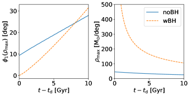
Figure 7: A comparison of the position of the peak of the linear density profile (left) and the peak density (right) for the noBH-QSG-AN (blue solid) and wBH-QSG-AN (orange dashed) models.

As seen in the left panel of Fig. 7, which displays the location of the peak of the linear density profile as a function of the time since dissolution for the QSG-AN models, the curves intersect at $t-t_{\rm d}\sim 8~{}{\rm Gyr}$ due to the combination of the location of the peak at dissolution and the growth rate of the streams. There exists such a point post-dissolution for all streams where the noBH and wBH cases cannot be distinguished based upon the position of the peak of the density profile. The time since dissolution at which this intersection happens is not just dependent on the initial mass, orbit, and choice of free parameters ($f_{\rm e}$ and $\epsilon$), but is a strong function of the choice of $\eta$ in the wBH and noBH cases (with a more positive $\eta$ resulting in a peak further along the stream and a more negative $\eta$ resulting in a peak closer to the progenitor’s position post-dissolution).

3.3 Central gap

The shape of the density profile of the gap from the progenitor’s position at the centre to the peak of the linear density profile has an asymmetric “S”-shape, as seen in Fig. 3. We define the shape of the linear density profile of the gap as the shape of the linear density profile from the centre to the peak of the linear density profile where $\phi_{1}$ and $\rho$ are normalised by the values of the peak. The shape of this curve is primarily dictated by the mass-loss rate of the progenitor but it has a secondary dependence on the mass of the retained BH population.

As a noBH progenitor approaches dissolution, the cluster mass tends to zero when the final stars are released and therefore so does the Jacobi radius and thereby the mean velocity and the dispersion of escapers. This results in the density profile gently increasing from the progenitor’s position towards the peak and, due to the decelerating mass-loss rate, the rate of increase will gently slow approaching the peak forming a more rounded shape than the wBH case (as seen in Fig. 3). With time since dissolution, differential streaming leads to the density profile widening and flattening, making the increase gentler with time.

In contrast, as a wBH progenitor approaches dissolution, the cluster mass tends to $M_{\rm BH}$ when the final stars are released and therefore the Jacobi radius is still at some distance and as a result the typical star will still have some significant velocity along the stream. In the wBH-QSG models $r_{\rm J}\simeq 14~{}{\rm pc}$ at dissolution, such that the final star escapes at a radial distance of $21~{}{\rm pc}$ from the centre of the cluster and, according to equation (14), has an average speed along the stream of $\sim 0.4~{}{\rm km/s}$ with respect to the progenitor assuming it has a velocity offset equal to the mean of the velocity distribution. In the wBH-Nbody model at dissolution, the average radial distance of stars within $50~{}{\rm pc}$ of the progenitor’s position is $\sim 15.7~{}{\rm pc}$, such that according to equation (14) (taking $\epsilon=f_{\rm e}=1$ for simplicity) these stars will have an average velocity of $\sim 0.35~{}{\rm km/s}$. This results in the density profile being initially flat before sharply rising towards the peak, as even the final stars are better able to keep pace with the stars that compose the peak. With time since dissolution the density profile flattens and widens, as in the noBH case, however the flat central section of the gap and steeper increase to the peak persists.

With decreasing $\eta$, the same portion of the progenitors mass is released in a shorter period before dissolution, this leads to a sharper peak with greater amplitude, as well as impacting the shape of the linear density profile of the gap. The flattening and widening of the density profile that occurs due to differential streaming, causes the shape of the linear density profile of the central gap to initially change but quickly tend to a near-constant shape.

In the $N$-body simulations we see that the gap contains more stars than predicted by QSG (see Fig. 3) making it more difficult to tell the two apart based on the shape of the gap alone. However, it is hoped that in the future wBH and noBH streams can be differentiated based on the shape of the gap. In addition, it is hoped that a gap due to a retained BH population can be differentiated from a gap due to a sub-halo flyby based on their distinct shapes.

The rate of growth of the central gap is dictated by the rate at which the stars that compose the end of the gap propagate away. Where exactly the end of the gap is defined to be is somewhat arbitrary. Here we define the end of the gap to be the peak of the linear density profile and as such we have assumed that there is an approximately equal inflow and outflow of mass in this region due to differential streaming, taking $M_{\rm gap}$ to be constant (this is accurate in the noBH case but in the wBH case the mass in this region doubles over the first $4~{}{\rm Gyr}$ post-dissolution). The average speed of a typical star ($\Delta v_{x}=\Delta v_{y}=0$) along the stream is dependent on the escape radius, $f_{\rm e}r_{\rm J}$, and the potential (through $\gamma$), such that (given our assumption) the gap grows at a rate that follows the relation

$$v_{\rm gap}\propto\Omega^{1/3}M_{\rm gap}^{1/3},$$ (15)

where $M_{\rm gap}$ is the sum of the stellar mass and the black hole mass. From this we can see that the BH population impacts the rate at which the gap opens in two ways. First, directly through $M_{\rm BH}$, but this impact is small as $M_{\rm gap}$ is much greater than $M_{\rm BH}$ in realistic cases. This impact is mostly seen in the final stars where the stellar and BH masses are comparable, leading to a flattening of the bottom of the linear density profile of the gap, as these stars can better keep pace with those that compose the peak, but does not noticeably impact the position of the peak for realistic $M_{\rm BH}$. Secondly, through the fact the BH population dictates the mass dependence of the mass-loss rate, $\eta$, which dictates where the position of peak and thereby how much stellar mass is contained in the gap. It is through this that $v_{\rm gap}$ is primarily impacted by the retained BH population.

3.4 Stream width and radial offset

To gain a sense of how the width and radial offset of a stream depend on the progenitor’s properties, these quantities can be estimated from $\Delta r$. As the typical star escapes with $\Delta v_{x}=\Delta v_{y}=0$, equation (6) reduces to

$$\Delta r=f_{\rm e}r_{\rm J}\left[\cos(\gamma\Omega t)+\frac{2}{\gamma^{2}}(1+\epsilon)\left(1-\cos(\gamma\Omega t)\right)\right].$$ (16)

The radial offset of the stream from the progenitor’s orbital track can be approximated as the average radial displacement of a typical star over time

$$\overline{\Delta r}=\frac{2}{\gamma^{2}}(1+\epsilon)f_{\rm e}r_{\rm J},$$ (17)

The width of the stream in the radial direction, $w_{x}$, can be approximated as twice a typical star’s mean displacement from $\overline{\Delta r}$,

$$w_{x}=2\langle|\Delta r-\overline{\Delta r}|\rangle=\frac{4}{\pi}\left[\frac{2}{\gamma^{2}}(1+\epsilon)-1\right]f_{\rm e}r_{\rm J},$$ (18)

For a progenitor on a circular orbit about a SIS potential these simply become $\overline{\Delta r}=(1+\epsilon)f_{\rm e}r_{\rm J}$, $w_{x}=\frac{4}{\pi}\epsilon f_{\rm e}r_{\rm J}$. This shows that the width and radial offset are dependent on the escape radius. Note, these expressions are the same as can be obtained from the equations of motion of Küpper et al. (2008) if $\epsilon=f_{\rm e}=1$.

For the assumptions we have made of a circular orbit about a spherical potential, Erkal et al. (2016) demonstrates that the width perpendicular to the orbital plane of the progenitor is determined by the spread in the stars orbital planes

$$w_{z}=\frac{\sigma}{\sqrt{2}\Omega},$$ (19)

where $\sigma$ is the velocity dispersion at the escape radius given by equation (10).

From this it is clear that, as seen in Figs. 4 & 5, wBH streams will be wider and more radially offset than noBH streams because of their greater initial mass. However, even if a wBH and noBH stream have the same initial mass, close to the progenitor the stream will still be wider and more radially offset due to the differing mass-loss rates causing the wBH cluster to contain more stellar mass at any fraction of its dissolution time.

From equation (17) it is seen that the clearest difference between the wBH and noBH cases is when the final stars escape. As mentioned in Section 3.3, the wBH cluster still has some finite mass $M_{\rm BH}$ when the last stars escape such that $r_{\rm J}>0$, whereas the noBH cluster has no mass and therefore $r_{\rm J}\simeq 0$. As a result, the stream is wider in the wBH case and more importantly it is radially offset from the progenitor’s orbital track. However, as time since dissolution increases, the innermost region of the stream will become dominated by the slowest stars, which lie approximately along the orbital track of the progenitor, as differential streaming becomes dominant. Resulting in this clear indicator of a retained BH population in the QSG framework being short-lived. In Fig. 8 this offset is clearly seen in the wBH-QGS-PS model due to the idealised escape conditions of the final stars, however it is not clear in the wBH-Nbody model. This suggests that the final stars no longer follow our prescription for the escape conditions.

Claydon et al. (2017) demonstrated that the velocity dispersion at the Jacobi radius is better fit by a $\sigma\propto M^{5/24}$ relation than the $\sigma\propto M^{1/3}$ relation of a Plummer model that we assume here, leading to a factor of $2$ increase in the velocity dispersion at $M\sim 10^{3}~{}{\rm M}_{\odot}$. In addition, approaching dissolution the ratio of half-mass radius to Jacobi radius is larger ($r_{\rm h}/r_{\rm J}\sim 0.3$) than our assumed value ($r_{\rm h}/r_{\rm J}\sim 0.15$) which would also increase the velocity dispersion. To test whether this resolves the disparity between the wBH-QGS-PS and wBH-Nbody models we increase $r_{\rm h}/r_{\rm J}$ from $0.15$ to $0.3$ smoothly over the last $0.1M_{\rm i}$ and increase $\sigma$ smoothly by a factor of $2$ over the last $0.2M_{\rm i}$ and observe that this increases the width of the central region of the stream as there is now a larger distribution in $\Delta v_{y}$ (see panel b of Fig. 8), however it does not reconcile the QSG-PS model with the $N$-body model. Adding a Gaussian scatter to the escape radius to the last $0.1M_{\rm i}$ improves the agreement with the $N$-body model (see panel c of Fig. 8), however we require for the escape radius to decrease $f_{\rm e}<1$ approaching dissolution to reproduce the smooth distribution of stars going from the leading to the trailing tail (see panel d of Fig. 8). This lower value of $f_{\rm e}$ can be understood from the fact that close to dissolution the low-mass cluster is dominated of stars with energies well above the critical energy for escape (so-called ‘potential escapers’, Fukushige & Heggie 2000), which have average distances from the cluster center of $\sim 0.5r_{\rm J}$ (Claydon et al., 2017) from which they are able to escape because of their high energy. However, there are still areas these refinements do not help. First, this better reproduction of the radial distribution of the central stars diminishes with time since dissolution. Second, the region enclosing central $500~{}{\rm M}_{\odot}$ (dashed line in Fig. 8) is much smaller than in the $N$-body model because our mass-loss rate diverges approaching dissolution due to its power-law nature. This suggests that, while refined escape conditions for the wBH model approaching dissolution may alleviate some of the discrepancy, there are other aspects of the model (such as the mass-loss rate) that also need refining. Even with these refinements, the simplistic nature of the QSG models may prevent it from accurately reproducing the distribution of stars in the central region and we therefore conclude that the radial offset from the orbital track can not be used to identify a surviving BH population in streams’ progenitors.

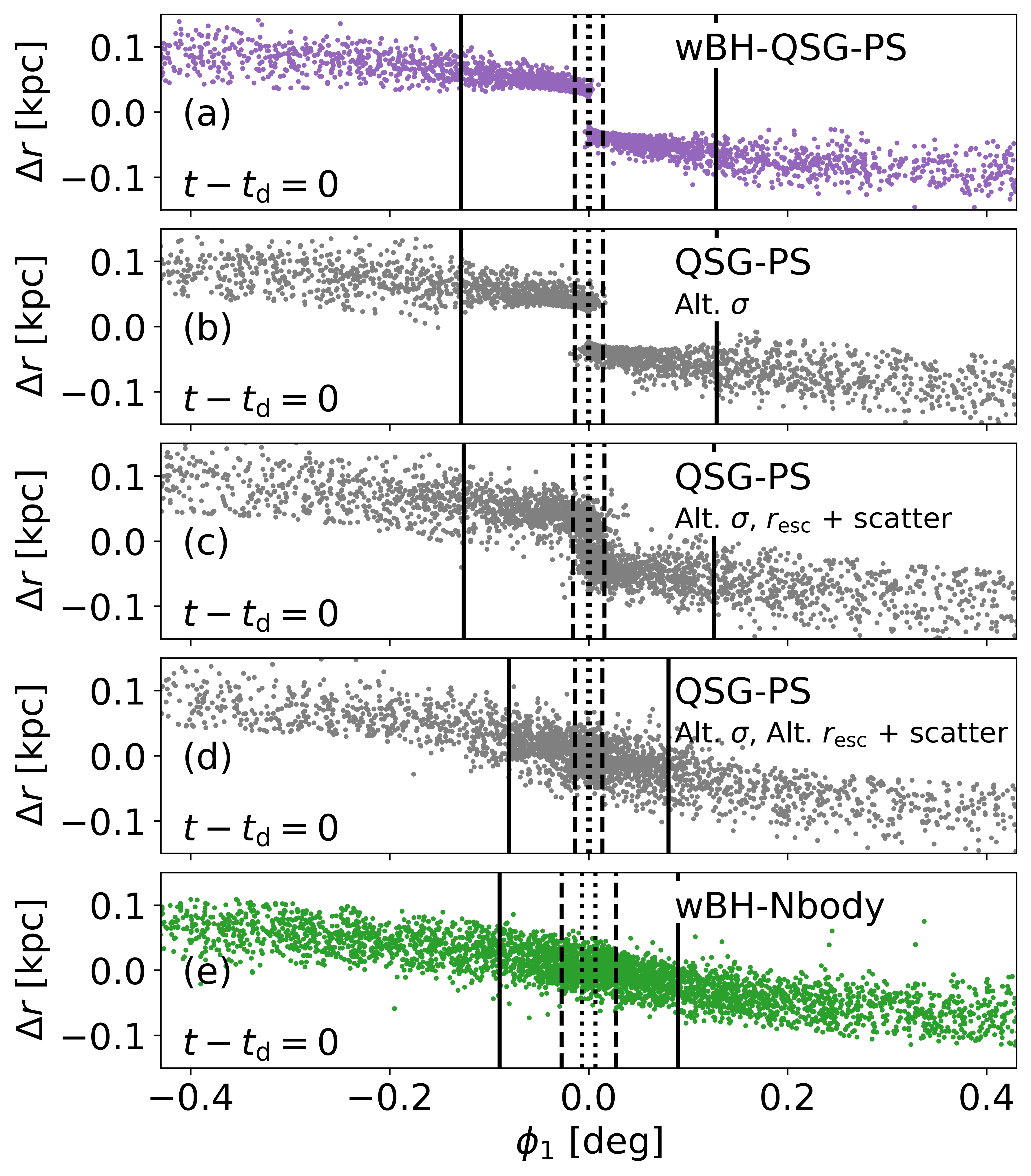
Figure 8: A comparison of the stream projections on to the orbital plane. The region $|\phi_{1}|\lesssim 0.43\degree$ ($0.15~{}{\rm kpc}$) is displayed at dissolution. In the central three panels (b,c,d) the escape conditions are altered from those described in section 2 (see text) to obtain a better agreement between wBH-QSG-PS and wBH-Nbody. The models displayed are, from top to bottom, (a) the wBH-QSG-PS model with the escape conditions described in section 2 (purple), (b) the wBH-QSG-PS model with increased velocity dispersion to better match the findings of Claydon et al. (2017), (c) the wBH-QSG-PS model with modified velocity dispersion and Gaussian scatter in the escape radius, (d) the wBH-QSG-PS model with modified velocity dispersion, decreasing escape radius, and Gaussian scatter in the escape radius, and (e) the wBH-Nbody model (green). The solid, dashed, and dotted vertical lines enclose the central $1000$, $500$, and $150~{}{\rm M}_{\odot}$ respectively.

4 Discussion

The first three tail properties discussed in Sections 3.1, 3.2 and 3.3 formally depend on the mass-loss rate and not directly on the BHs, meaning that alternative scenarios that lead to similar mass-loss histories (such as a low initial cluster density, G21) might result in similar stream properties. This means that finding such tail properties is a necessary, but not sufficient, condition for the presence of BHs. However, G21 show that the region in parameter space (low initial density and high initial mass) of clusters without BHs that have similarly high mass-loss rate is extremely small and this ‘fine-tuning’ problem makes the BH hypothesis a more likely scenario. We therefore conclude that if the tails suggest that the progenitor had a high mass-loss rate, the most likely interpretation is that the progenitor was rich in BHs.

One of the advantages of the QSG models that we present here is the speed at which they can generate realistic streams / density profiles, taking less than $0.01~{}{\rm s}$ for as single snapshot of wBH-QSG-AN/PS (including generating the initial conditions for QSG-PS). The speed of these models allows for quick exploration of parameter space compared to $N$-body models. These models are not just limited to investigating the impact of mass-loss rate on stream structure. The QSG models could potentially be used in conjunction with the equations of motion from Erkal & Belokurov (2015) for stars after a dark matter subhalo (DMSH) fly-by to quickly narrow down the parameter space of the DMSH from the properties of the gap left behind.

The QSG-PS and QSG-AN models are able to quickly produce realistic streams and density profiles prior- or post-dissolution for both the noBH and wBH cases, as seen in Figs. 3, 4, & 5. There are, however, a few aspects of the streams structure that QSG-PS does not capture well. Namely, the distribution in the $\phi_{1}$-$\Delta z$ plane and the distribution of central stars near the progenitor cluster post-dissolution which both require the implementation of more realistic escape conditions. Further refinement with the implementation of a more realistic velocity distribution of escapers such as that of Claydon et al. (2017), a time varying $M_{\rm BH}$, and a refined prescription of escape conditions following a study of stars escaping wBH GCs approaching dissolution (which may call for a time varying $f_{\rm e}$) would greatly reduce these discrepancies making the insights gleaned from these models more reliable and impactful.

Our model is only valid for streams on circular orbits, but those on low eccentricity orbits can be approximated using a circular orbit of equal period with radius $R_{\rm T}$ and minimising the effect of the periodic stretching and compression due to the eccentricity by multiplying $\phi_{1}$ by $R(t)^{2}/R_{\rm T}^{2}$. For a Kepler orbit $R_{\rm T}$ is the semi-major axis and this approximation is within $1\%$ ($10\%$) of the azimuthal period for orbits with eccentricities below $\sim 0.25$ ($0.75$) in a SIS. The expected orbit-averaged mass-loss rate for eccentric orbits can be calculated using an equivalent circular orbit with the same mass-loss rate (see Baumgardt & Makino, 2003), which does not include any enhancement/reduction in mass-loss at peri-/apo-galacticon. This is important as GCs typically exist on eccentric orbits (Odenkirchen et al., 1997; van den Bosch et al., 1999) and through this methodology not only can we project streams onto circular orbits to compare to the QSG models, but we can project the QSG models onto eccentric orbits allowing us to escape the confines of the circular orbit case.

The easiest approach to extend the model to eccentric orbits is with the QSG-PS model. The model parameters $\epsilon$ and $f_{\rm e}r_{\rm J}$ may need to be redetermined and may depend on eccentricity and/or the Galactic potential. A model for eccentric orbit can be deployed to directly infer the model parameters $\eta$, $M_{\rm i}$ from stream density profiles such as the ones presented in Patrick et al. (2022). Other improvements include the preferential escape of low-mass stars and variations in the stellar mass function which when combined with deep photometry of streams can provide additional constraints on the initial mass function (IMF) of GCs in addition to IMF constraints from mass modelling of GCs (Baumgardt et al., 2023; Dickson et al., 2023).

5 Conclusions

In this work we present a semi-analytical model of stream formation from star clusters on circular orbits and with time-dependent mass-loss rates and demonstrate that it produces streams that are in good agreement with $N$-body simulations of streams. The model has three free parameters that we determine from the comparison with the $N$-body models: (i) the mass dependency of the mass-loss rate, $\eta$, (ii) the mean distance of escape, $f_{\rm e}r_{\rm J}$, and (iii) the relation between the escape radius and the centre of the velocity distribution, $\epsilon$. The best fit values are found to be $\epsilon\simeq 0.57$ and $f_{\rm e}\simeq 1.5$ for our choice of initial mass. We then compare the structure of streams resulting from progenitors that retain a stellar-mass black hole population (wBH) and those that do not (noBH). Retention of a stellar-mass BH population leads to streams that are more massive, have a peak closer to the progenitor location, have a narrower peak, and are more radially offset from the orbit. This is because, due to their accelerating mass-loss rate, wBH streams have approximately five times the mass of the equivalent noBH stream. It is also found that the shape of the central gap in the linear density profile is dependent on the mass-loss rate, and thereby the retained BH population.

We also show that the limit on the mass of a noBH GC that can dissolve in a given time on a given orbit (Baumgardt & Makino 2003; GG23) can be used to show that 5 of the 7 streams (that are believed to have originated from GCs) included in Patrick et al. (2022) have a mass that exceeds the initial mass of a noBH GC on an equivalent circular orbit that can dissolve in $10~{}{\rm Gyr}$ (see Fig. 1). Not only does the orbit place a limit upon the mass in the stream, but also on the linear density, such that you do not necessarily need to observe the whole stream to find the mass within to be inconsistent with a noBH progenitor. This opens a new avenue to use the plethora of stellar streams without progenitors to learn about the black hole content of their dissolved progenitors.

Data Availability

The data underlying this article will be shared on reasonable request to the corresponding authors.

Appendix A Deriving the Equation of Motion

Here a derivation of the equations of motion of escaped stars in the cluster centred frame from section 2.3 is presented. Using the common substitution $u=1/R$ and expanding the equations of motion at leading order gives

$$\frac{{\rm d}^{2}\Delta u}{{\rm d}\theta^{2}}+\gamma^{2}\Delta u=-2u_{0}\left(\frac{\Delta v_{y}}{V_{\rm c}}+\frac{f_{\rm e}r_{\rm J}}{R}\right)$$ (20)

where $\theta$ is the azimuthal angle about the galactic centre and

$$\gamma^{2}=3+\frac{R^{2}}{V_{\rm c}^{2}}\partial_{R}^{2}\Phi.$$ (21)

The corresponding initial conditions of $u$ are given by $\Delta u(0)=-f_{\rm e}r_{\rm J}/R^{2}$ and $\partial_{\theta}\Delta u(0)=-u\Delta v_{x}/V_{\rm c}$. Giving a solution to equation (20) of

$$\begin{array}[]{ll}\Delta u=&-\frac{f_{\rm e}r_{\rm J}}{R^{2}}\cos(\gamma\theta)-\frac{2u_{0}}{\gamma^{2}}\left[\frac{\Delta v_{y}}{V_{\rm c}}+\frac{f_{\rm e}r_{\rm J}}{R}\right]\left[1-\cos(\gamma\theta)\right]\\ &-\frac{u_{0}\Delta v_{x}}{V_{\rm c}}\frac{\sin(\gamma\theta)}{\gamma}.\end{array}$$ (22)

Switching back from $u$ to $R$

$$\begin{array}[]{ll}\Delta R=&f_{\rm e}r_{\rm J}\cos(\gamma\theta)-\frac{2R}{\gamma^{2}}\left[\frac{\Delta v_{y}}{V_{\rm c}}+\frac{f_{\rm e}r_{\rm J}}{R}\right]\left[1-\cos(\gamma\theta)\right]\\ &-\frac{R\Delta v_{x}}{V_{\rm c}}\frac{\sin(\gamma\theta)}{\gamma}.\end{array}$$ (23)

Using conservation of angular momentum

$$L_{z}=R^{2}\dot{\theta},$$ (24)

$\dot{\theta}$ can be expressed as

$$\begin{array}[]{ll}\dot{\theta}=&\frac{V_{\rm c}}{R}\left[1-\left(\frac{\Delta v_{y}}{V_{\rm c}}+\frac{f_{\rm e}r_{\rm J}}{R}\right)\left(\frac{4-\gamma^{2}}{\gamma^{2}}\right)\right.\\ &\left.-2\left(\frac{f_{\rm e}r_{\rm J}}{R}\frac{\gamma^{2}-2}{\gamma^{2}}-\frac{2}{\gamma^{2}}\frac{\Delta v_{y}}{V_{\rm c}}\right)\cos(\gamma\theta)-2\frac{\Delta v_{x}}{V_{\rm c}}\frac{\sin(\gamma\theta)}{\gamma}\right].\end{array}$$ (25)

Integrating over $t$, and approximating $\theta$ as $V_{\rm c}t/R$ at leading order, the angular displacement relative to the progenitor can be expressed as

$$\begin{array}[]{ll}\phi_{1}(t,\Delta v_{x},\Delta v_{y})=&-\frac{4-\gamma^{2}}{\gamma^{2}}\left(\frac{\Delta v_{y}}{V_{\rm c}}+\frac{f_{\rm e}r_{\rm J}}{R}\right)\frac{V_{\rm c}t}{R}\\ &-\frac{2}{\gamma^{3}}\left((\gamma^{2}-2)\frac{f_{\rm e}r_{\rm J}}{R}-\frac{2\Delta v_{y}}{V_{\rm c}}\right)\sin\left(\frac{\gamma V_{\rm c}t}{R}\right)\\ &-\frac{2\Delta v_{x}}{V_{\rm c}}\frac{1-\cos\left(\frac{\gamma V_{\rm c}t}{R}\right)}{\gamma^{2}}.\end{array}$$ (26)

This expression gives the angular displacement of a particle from the progenitor as a function of time and the escape conditions. Since the Lagrange points move at the same angular rate as the progenitor (for a circular orbit), the mean velocity at the Lagrange point can be related to the radial offset through a free parameter $\epsilon$

$$\frac{\Delta v_{y}}{V_{\rm c}}\rightarrow\epsilon\frac{f_{\rm e}r_{\rm J}}{R}+\frac{\Delta v_{y}}{V_{\rm c}},$$ (27)

where $\Delta v_{y}$ is now the random component of the velocity with a mean of zero. $\epsilon=1$ for a constant angular rate. Re-writing $\Delta r$ and $\phi_{1}$

$$\begin{array}[]{ll}\phi_{1}(t)=&-\frac{4-\gamma^{2}}{\gamma^{2}}\left(\Delta v_{y}+(1+\epsilon)\frac{f_{\rm e}r_{\rm J}}{R}V_{\rm c}\right)\frac{t}{R}\\ &-\frac{2}{\gamma^{3}}(\gamma^{2}-2-2\epsilon)\frac{f_{\rm e}r_{\rm J}}{R}\sin\left(\gamma\frac{V_{\rm c}}{R}t\right)\\ &+\frac{1}{\gamma^{3}}\frac{4\Delta v_{y}}{V_{\rm c}}\sin\left(\gamma\frac{V_{\rm c}}{R}t\right)\\ &-\frac{1}{\gamma^{2}}\frac{2\Delta v_{x}}{V_{\rm c}}\left(1-\cos\left(\gamma\frac{V_{\rm c}}{R}t\right)\right),\end{array}$$ (28)

$$\begin{array}[]{ll}\Delta r(t)=&f_{\rm e}r_{\rm J}\cos(\gamma\phi_{1})+\frac{2R}{\gamma^{2}}\left(\frac{\Delta v_{y}}{V_{\rm c}}+(1+\epsilon)\frac{f_{\rm e}r_{\rm J}}{R}\right)\times\\ &\left(1-\cos(\gamma\phi_{1})\right)+\frac{R\Delta v_{x}}{V_{\rm c}}\frac{\sin(\gamma\phi_{1})}{\gamma},\end{array}$$ (29)

where we have changed $\Delta R$ to $\Delta r$ to signify that, in the context of this work, we are considering it as the displacement from the progenitor’s orbital track in a cluster centred frame rather than the change in galactocentric radius in the galactocentric frame, of course the two are equivalent in this model restricted to circular orbits.

References

- Balbinot et al. (2022) Balbinot E., Cabrera-Ziri I., Lardo C., 2022, MNRAS, 515, 5802
- Banerjee & Kroupa (2011) Banerjee S., Kroupa P., 2011, ApJ, 741, L12
- Banerjee et al. (2020) Banerjee S., Belczynski K., Fryer C. L., Berczik P., Hurley J. R., Spurzem R., Wang L., 2020, Astronomy & Astrophysics, 639, A41
- Baumgardt (2001) Baumgardt H., 2001, MNRAS, 325, 1323
- Baumgardt & Makino (2003) Baumgardt H., Makino J., 2003, MNRAS, 340, 227
- Baumgardt et al. (2023) Baumgardt H., Hénault-Brunet V., Dickson N., Sollima A., 2023, MNRAS, 521, 3991
- Belokurov et al. (2006) Belokurov V., et al., 2006, ApJ, 642, L137
- Bernard et al. (2016) Bernard E. J., et al., 2016, MNRAS, 463, 1759
- Bonaca et al. (2020) Bonaca A., et al., 2020, The Astrophysical Journal, 892, L37
- Bonaca et al. (2021) Bonaca A., et al., 2021, ApJ, 909, L26
- Bovy (2014) Bovy J., 2014, ApJ, 795, 95
- Bovy (2015) Bovy J., 2015, The Astrophysical Journal Supplement Series, 216, 29
- Bovy et al. (2016) Bovy J., Bahmanyar A., Fritz T. K., Kallivayalil N., 2016, ApJ, 833, 31
- Breen & Heggie (2013) Breen P. G., Heggie D. C., 2013, Monthly Notices of the Royal Astronomical Society, 432, 2779
- Claydon et al. (2017) Claydon I., Gieles M., Zocchi A., 2017, Monthly Notices of the Royal Astronomical Society, 466, 3937
- Dickson et al. (2023) Dickson N., Hénault-Brunet V., Baumgardt H., Gieles M., Smith P. J., 2023, MNRAS, 522, 5320
- Erkal & Belokurov (2015) Erkal D., Belokurov V., 2015, Monthly Notices of the Royal Astronomical Society, 450, 1136
- Erkal et al. (2016) Erkal D., Sanders J. L., Belokurov V., 2016, Monthly Notices of the Royal Astronomical Society, 461, 1590
- Erkal et al. (2019) Erkal D., et al., 2019, MNRAS, 487, 2685
- Fardal et al. (2015) Fardal M. A., Huang S., Weinberg M. D., 2015, MNRAS, 452, 301
- Ferguson et al. (2022) Ferguson P. S., et al., 2022, AJ, 163, 18
- Fryer et al. (2012) Fryer C. L., Belczynski K., Wiktorowicz G., Dominik M., Kalogera V., Holz D. E., 2012, The Astrophysical Journal, 749, 91
- Fukushige & Heggie (2000) Fukushige T., Heggie D. C., 2000, MNRAS, 318, 753
- Gibbons et al. (2014) Gibbons S. L. J., Belokurov V., Evans N. W., 2014, MNRAS, 445, 3788
- Gieles & Gnedin (2023) Gieles M., Gnedin O. Y., 2023, MNRAS, 522, 5340 (GG23)
- Gieles et al. (2021) Gieles M., Erkal D., Antonini F., Balbinot E., Peñarrubia J., 2021, Nature Astronomy, 5, 957 (G21)
- Giersz et al. (2019) Giersz M., Askar A., Wang L., Hypki A., Leveque A., Spurzem R., 2019, MNRAS, 487, 2412
- Grillmair & Dionatos (2006) Grillmair C. J., Dionatos O., 2006, ApJ, 643, L17
- Hénon (1961) Hénon M., 1961, Ann. Astrophys., 24, 369
- Hurley et al. (2000) Hurley J. R., Pols O. R., Tout C. A., 2000, Monthly Notices of the Royal Astronomical Society, 315, 543
- Hurley et al. (2002) Hurley J. R., Tout C. A., Pols O. R., 2002, Monthly Notices of the Royal Astronomical Society, 329, 897
- Ibata et al. (1994) Ibata R. A., Gilmore G., Irwin M. J., 1994, Nature, 370, 194
- Ibata et al. (2001) Ibata R., Irwin M., Lewis G., Ferguson A. M. N., Tanvir N., 2001, Nature, 412, 49
- Ibata et al. (2018) Ibata R. A., Malhan K., Martin N. F., Starkenburg E., 2018, The Astrophysical Journal, 865, 85
- Ibata et al. (2019) Ibata R. A., Malhan K., Martin N. F., 2019, ApJ, 872, 152
- Koposov et al. (2010) Koposov S. E., Rix H.-W., Hogg D. W., 2010, ApJ, 712, 260
- Koposov et al. (2014) Koposov S. E., Irwin M., Belokurov V., Gonzalez-Solares E., Yoldas A. K., Lewis J., Metcalfe N., Shanks T., 2014, MNRAS, 442, L85
- Koposov et al. (2023) Koposov S. E., et al., 2023, MNRAS, 521, 4936
- Kroupa (2001) Kroupa P., 2001, Monthly Notices of the Royal Astronomical Society, 322, 231
- Küpper et al. (2008) Küpper A. H., Macleod A., Heggie D. C., 2008, Monthly Notices of the Royal Astronomical Society, 387, 1248
- Küpper et al. (2010) Küpper A. H. W., Kroupa P., Baumgardt H., Heggie D. C., 2010, Monthly Notices of the Royal Astronomical Society, 401, 105–120
- Küpper et al. (2015) Küpper A. H. W., Balbinot E., Bonaca A., Johnston K. V., Hogg D. W., Kroupa P., Santiago B. X., 2015, ApJ, 803, 80
- Kuzma et al. (2018) Kuzma P. B., Da Costa G. S., Mackey A. D., 2018, MNRAS, 473, 2881
- Lamers et al. (2010) Lamers H. J. G. L. M., Baumgardt H., Gieles M., 2010, MNRAS, 409, 305
- Li et al. (2022) Li T. S., et al., 2022, ApJ, 928, 30
- Lynden-Bell & Lynden-Bell (1995) Lynden-Bell D., Lynden-Bell R. M., 1995, MNRAS, 275, 429
- Malhan et al. (2018) Malhan K., Ibata R. A., Martin N. F., 2018, MNRAS, 481, 3442
- Martin et al. (2022) Martin N. F., et al., 2022, Nature, 601, 45
- Martínez-Delgado et al. (2010) Martínez-Delgado D., et al., 2010, AJ, 140, 962
- Martínez-Delgado et al. (2023) Martínez-Delgado D., et al., 2023, A&A, 671, A141
- Newberg et al. (2010) Newberg H. J., Willett B. A., Yanny B., Xu Y., 2010, ApJ, 711, 32
- Odenkirchen et al. (1997) Odenkirchen M., Brosche P., Geffert M., Tucholke H. J., 1997, New Astron., 2, 477
- Odenkirchen et al. (2001) Odenkirchen M., et al., 2001, ApJ, 548, L165
- Patrick et al. (2022) Patrick J. M., Koposov S. E., Walker M. G., 2022, MNRAS, 514, 1757
- Pavlík et al. (2018) Pavlík V., Jeřábková T., Kroupa P., Baumgardt H., 2018, A&A, 617, A69
- Plummer (1911) Plummer H. C., 1911, Monthly Notices of the Royal Astronomical Society, 71, 460
- Sanders (2014) Sanders J. L., 2014, MNRAS, 443, 423
- Shipp et al. (2018) Shipp N., et al., 2018, ApJ, 862, 114
- Wang (2020) Wang L., 2020, MNRAS, 491, 2413
- Wang et al. (2020) Wang L., Iwasawa M., Nitadori K., Makino J., 2020, Monthly Notices of the Royal Astronomical Society, 497, 536
- Wang et al. (2024) Wang L., Gieles M., Baumgardt H., Li C., Pang X., Tang B., 2024, MNRAS, 527, 7495
- de Boer et al. (2020) de Boer T. J. L., Erkal D., Gieles M., 2020, MNRAS, 494, 5315
- van den Bosch et al. (1999) van den Bosch F. C., Lewis G. F., Lake G., Stadel J., 1999, ApJ, 515, 50