A glance at evolvability: a theoretical analysis of its role in the evolutionary dynamics of cell populations

Abstract

Evolvability is defined as the ability of a population to generate heritable variation to facilitate its adaptation to new environments or selection pressures. In this article, we consider evolvability as a phenotypic trait subject to evolution and discuss its implications in the adaptation of cell populations. We explore the evolutionary dynamics of an actively proliferating population of cells subject to changes in their proliferative potential and their evolvability using a stochastic individual-based model and its deterministic continuum counterpart through numerical simulations of these models. We find robust adaptive trajectories that rely on cells with high evolvability rapidly exploring the phenotypic landscape and reaching the proliferative potential with the highest fitness. The strength of selection on the proliferative potential, and the cost associated with evolvability, can alter these trajectories such that, if both are sufficiently constraining, highly evolvable populations can become extinct in our individual-based model simulations. We explore the impact of this interaction at various scales, discussing its effects in undisturbed environments and also in disrupted contexts, such as cancer.

Keywords— Evolutionary dynamics, Mathematical modeling, Phenotypically-structured populations,
Evolvability

Corresponding author— Juan Jiménez-Sánchez (juan.jsanchez@uclm.es)

1 Introduction

In nature, variation in phenotypic traits and selection are the general conditions for evolution to occur [1, 2, 3, 4]. Selection acts on phenotypic variants to promote the prevalence of the fittest. The greater the diversity within a population, the higher its chances of withstanding the pressures imposed by selective agents [5]. Phenotypic variability is generated by a plethora of biological mechanisms, most of which operate at the cellular level, but whose effects are manifested at the macroscopic level [6]. Arguably the mechanism that operates at the most fundamental level is mutation. The stochastic nature of mutations, as well as their high occurrence [7], results in the generation of both detrimental and beneficial variants. According to recent studies on the distribution of fitness effects, although detrimental variants are more frequent [8], beneficial mutations must be present for adaptation to occur [9]. This ability to generate variability on which selection can act upon is known as evolvability [10].

More formally, evolvability can be defined as a population’s capacity to provide adaptive and heritable phenotypic variation amongst its individuals, to let them evolve and overcome selective pressures. The above definition could be considered a consensus of overlapping ideas amongst different evolutionary biologists, as each brings a different nuance depending on their concept of evolvability and the scale at which they study it [10, 11, 12, 13]. It could be argued that greater evolvability implies greater selective advantage, as the adaptive potential increases the likelihood of surviving selective pressures. However, different ecological scenarios may foster populations with lower evolvability [14]; e.g. a population that is already very well adapted to its environment may not need a high capacity to generate variability. In nature, the actual interplay between a population’s evolvability and its environment may be much more intricate, giving rise to more complex strategies, such as bet-hedging: increasing phenotypic variation may reduce fitness in the current environment, but maximizes the chances of survival in the face of changes in that environment [15, 16, 17].

Evolvability itself may be evolvable and subject to change over time [12], suggesting that it should also be considered as a phenotypic trait [18]. Although the actual mechanisms that generate the trait of evolvability are unknown, several phenomena that influence it, and operate at different scales, can be surmised [11]. At the molecular level, nucleic acids and proteins, as biological systems, are subject to evolution themselves. Hence, alterations enhancing mutation rates may increase evolvability [19]. However, the deleterious nature of many mutations forces these biological systems to remain robust and preserve their sequence so that their structure is not altered and their function is not diminished. A balance between robustness and evolvability is therefore required, so that new sequences can be explored without detrimentally affecting essential features [11]. The relationship between robustness and evolvability of transcription factor binding sites in mice and yeast has been characterized [20], and evolvability-enhancing mutations were recently described in the context of RNA and proteins [21].

At the cellular level, the observed cell-to-cell variability has traditionally been ascribed on genetic variation [22], and also on epigenetic variation [23]. However, the stochastic nature of the biochemical processes taking place within the cell (such as noisy gene expression [24, 25] and errors in protein synthesis [26], as demonstrated recently by single-cell technologies [6, 27, 28, 29]) brings into play a non-genetic heterogeneity [30] which, together with the previous factors, is responsible for the emergence of phenotypic variation [31] and manifests itself as variations in cell size, function, lifespan, protein level, etc. A greater phenotypic variation may promote evolvability, according to experiments performed in yeast [32]. Hence, the genetic pathways that are involved in genomic repair, genomic instability, recombination (or, in the case of asexual populations, horizontal gene transfer), and regulation of gene expression (transcription factors, epigenetic modifications, etc) are likely to influence the level of evolvability. So far, evolvability-enhancing mutations have been described in bacteria and yeast [21]. Moreover, some theoretical studies have addressed the evolution of evolvability in gene regulatory networks [33, 34].

On a broader scale, several ecological factors, while not directly causing evolvability, influence the degree to which it becomes evident within a population. These factors encompass environmental stimuli, interactions amongst individuals within the same population, ecological dynamics between individuals in different populations, and varying selection pressures. Their interplay results in the creation of an adaptive landscape, which the population traverses in its quest for a global (or local) optimum. Thus far, only a limited number of theoretical works have addressed these adaptive dynamics while considering the concept of evolvability [14, 33, 35, 36].

Our aim is to carry out a theoretical study of the effect of evolvability on the adaptive dynamics of phenotypically-structured cell populations. Although we will focus on the case of cells, the model is general enough to consider any population of autonomous self-replicating agents subject to evolution, such as multicellular organisms. We will use stochastic individual-based (IB) models and corresponding deterministic continuum models, which we derive from the former using formal limiting procedures. The former are able to capture the stochastic nature of the phenotypic changes that may occur within individuals of the same population, hence recapitulating phenomena observed in the presence of small numbers of individuals such as genetic drift, while the latter provide a concise depiction of the collective behaviour of large numbers of individuals, thus making it possible to explore the adaptive trajectories of a whole population.

In this paper, we build upon earlier studies that addressed the evolutionary dynamics of phenotypically-structured populations [37, 38, 39, 40, 41] and non-genetic stochastic changes in cellular traits [42]. First of all, we expand the notion of populations with fluctuations in the characteristics considered in [39], so that we include evolvability as a continuous phenotypic trait. In the context of the model, evolvability is defined as the degree of variability in proliferative potential, such that an individual with higher evolvability will be more likely to undergo phenotypic changes in their proliferative potential than one with lower evolvability. Taking this information into consideration, and following the idea presented in [42], since evolvability is considered as a phenotypic trait per se, it is also subject to spontaneous heritable changes. Hence, we let the evolvability of a cell be itself subject to evolutionary change. In this way, we can explore the effect of non-genetic heterogeneity on the evolutionary dynamics of a phenotypically diverse population subject to varying adaptive potential, considering also fitness costs and selection pressures.

2 Materials and methods

2.1 The IB model

We develop an IB model for the evolutionary dynamics of a phenotypically heterogeneous population consisting of cells. We will use cells from now on, although this definition can be generalised to agents, so that agent can mean any self-replicating individual. The phenotypic state of every cell at time $t\in[0,t_{f}]$ is characterised by the structuring variables $y\in[0,1]$ and $x\in[0,1]$, which take into account intercellular variation in proliferative potential and evolvability, respectively. Without loss of generality, we focus on the case where larger values of y correspond to a higher cell division rate (i.e. a higher proliferative potential), and larger values of x correspond to a higher probability for changes in proliferative potential to occur (i.e. a higher evolvability). The variable $y$ could represent the normalised level of expression of a gene that regulates cell division – such as MKI67, BIRC5, CCNB1, CDC20, CEP55, NDC80, TYMS, NUF2, UBE2C, PTTG1, and RRM2 [43, 44, 45], while the variable $x$ could relate to the degree of variation of the level of expression of such a gene over time and, therefore, could be connected with the normalised level of expression of a gene that controls the expression of genes regulating cell division – such as FOXM1, MYBL2 or TOP2A [44, 46].

In order to define an on-lattice model, we discretise the time and phenotype variables. The current time step $t_{h}$ indicates how many steps $h$ of length $\Delta t$ have already been taken. Cells will be characterised by their phenotypic state ($y_{i},x_{j}$), which is represented as a position on the lattice $\{y_{i}\}_{i}\times\{x_{j}\}_{j}$ corresponding to phenotypic space $[0,1]\times[0,1]$. Cells can change their proliferative potential by taking $i$ steps of length $\Delta y$ (only one per time step), as well as their evolvability, by taking $j$ steps of length $\Delta x$ (also, only one per time step).

We introduce the variable $\mathcal{N}_{i,j}^{h}$ to model the number of cells in the phenotypic state ($y_{i},x_{j}$) at time $t_{h}$. From $\mathcal{N}_{i,j}^{h}$, we can calculate the cell population density $n_{i,j}^{h}$ (i.e. the phenotypic distribution of the cells) and the corresponding cell population size $N^{h}$ (i.e. the total number of cells) at time $t_{h}$. To keep track of the evolution of the phenotypic state, we define the mean level of proliferative potential $\bar{y}^{h}$ and the mean level of evolvability $\bar{x}^{h}$ (as well as their corresponding standard deviations $\sigma_{y}^{h}$ and $\sigma_{x}^{h}$). Hence, the point $(\bar{y}^{h},\bar{x}^{h})$ represents the mean phenotypic state of the cell population at time $t^{h}$.

Time and phenotypic variables are discretised according to

$$t_{h}=h\Delta t\in[0,t_{f}],\;\;y_{i}=i\Delta y\in[0,1]\;\text{ and }x_{j}=j\Delta x\in[0,1]\;\;\text{ with }\;h,i,j\in\mathbb{Z}^{+},\;\Delta t,\Delta y,\Delta x\in\mathbb{R}^{+}_{*},$$

where $\mathbb{Z}^{+}$ denotes the set of nonnegative integers and $\mathbb{R}^{+}_{*}$ denotes the set of strictly positive real numbers. The cell population density and the corresponding cell population size are computed via the following formulas

$$n_{i,j}^{h}\equiv n(t_{h},y_{i},x_{j}):=\frac{\mathcal{N}_{i,j}^{h}}{\Delta y\Delta x}\quad\text{and}\quad N^{h}\equiv N(t_{h}):=\sum_{i,j}\mathcal{N}_{i,j}^{h},$$ (1)

while the mean level of proliferative potential and the mean level of evolvability of the cell population at time $t_{h}$, along with the corresponding standard deviations, are computed according to

$$\bar{y}(t_{h})\equiv\bar{y}^{h}:=\frac{1}{N^{h}}\sum_{i,j}\mathcal{N}_{i,j}^{h}y_{i},\quad\sigma_{y}(t_{h})\equiv\sigma_{y}^{h}:=\left(\frac{1}{N^{h}}\sum_{i,j}\mathcal{N}_{i,j}^{h}y_{i}^{2}-\left(\bar{y}^{h}\right)^{2}\right)^{1/2}$$ (2)

and

$$\bar{x}(t_{h})\equiv\bar{x}^{h}:=\frac{1}{N^{h}}\sum_{i,j}\mathcal{N}_{i,j}^{h}x_{j},\quad\sigma_{x}(t_{h})\equiv\sigma_{x}^{h}:=\left(\frac{1}{N^{h}}\sum_{i,j}\mathcal{N}_{i,j}^{h}x_{j}^{2}-\left(\bar{x}^{h}\right)^{2}\right)^{1/2}.$$ (3)

As summarised by the schematics in Figure 1, between time-steps $h$ and $h+1$, each cell in phenotypic state $(y_{i},x_{j})$ can first undergo heritable, spontaneous phenotypic changes and then die, divide, or stay quiescent according to the rules described in the following subsections.

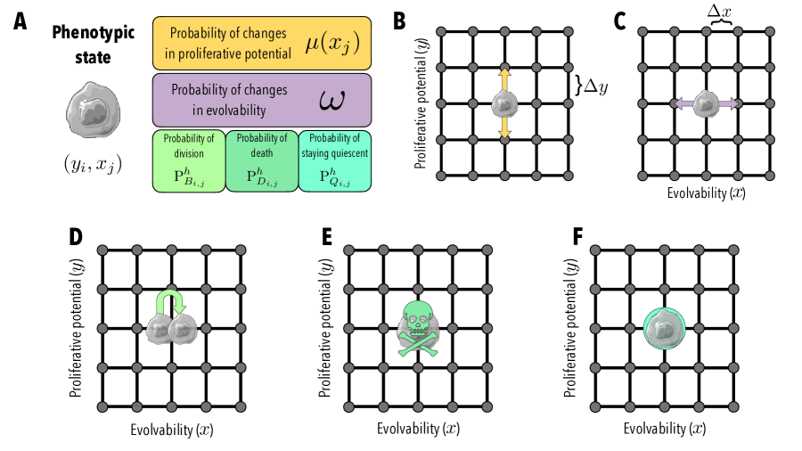
Figure 1: Schematic depiction of the basic processes a cell can undergo in the IB model. A A cell is characterised by its phenotypic state $(y_{i},x_{j})$, a pair of values of proliferative potential $y_{j}$ and evolvability $x_{i}$ that determine a position in the lattice $\{y_{i}\}_{i}\times\{x_{j}\}_{j}$, which defines the phenotypic space. Each phenotypic state $(y_{i},x_{j})$ is associated with a division probability $P_{B_{i},j}^{h}$ and a probability of change in proliferative potential $\mu(x_{j})$ (respectively). The different processes that a cell may undergo between time-steps $h$ and $h+1$ are summarized in the color boxes, and detailed hereafter. B Cells may undergo spontaneous phenotypic changes that increase or decrease their proliferative potential, according to a probability $\mu(x_{i})$ that depends on their level of evolvability. C Cells may also undergo spontaneous phenotypic changes that increase or decrease their level of evolvability, according to a fixed probability $\omega$. Increasing or decreasing the proliferative potential and the level of evolvability is equiprobable. D Cells may divide according to a probability ${\rm P}_{B_{i,j}}^{h}$ (cf. Eq. (6)). The newborn cell inherits the same phenotypic state as its parent. E Cells may die with a probability ${\rm P}_{D_{i,j}}^{h}$ (cf. Eq. (7)). Both division and death probabilities depend on a cell’s levels of proliferative potential and evolvability. F Cells may remain quiescent with a probability ${\rm P}_{Q_{i,j}}^{h}$ (cf. Eq. (8)).

2.1.1 Mathematical modelling of cell division and death

We assume that a dividing cell is instantly replaced by two identical cells that inherit the phenotypic state of the parent cell (i.e. the progenies are placed on the same lattice site as their parent), while a dying cell is instantly removed from the population. We model saturating growth of the cell population by letting the cells divide, die or remain quiescent with probabilities that depend on their phenotypic state and the cell population size. In particular, to define the probabilities of cell division and death, we introduce the function $R\equiv R(y_{i},x_{j},N^{h})$, which describes the net division rate (i.e. the difference between the rate of division and the rate of death) of cells in the phenotypic state $(y_{i},x_{j})$ under the environmental conditions corresponding to the cell population size $N^{h}$. In particular, we will focus on the case where:

$$R:=\rho(x,y)-\kappa\,N.$$ (4)

The definition given by Eq. (4) relies on the following assumptions: cells die due to intra-population competition at a rate proportional to the size of the cell population, with constant of proportionality $\kappa>0$; and cells in the phenotypic state $(y,x)$ divide and die due to natural selection on the proliferative potential at rate $\rho(x,y)$ (i.e. $\rho(x,y)$ is the intrinsic net division rate of cells in the phenotypic state $(y,x)$). In the framework of our model, under the definition given by Eq. (4), the function $\rho(x,y)$ determines the shape of the phenotypic fitness landscape of the cell population.

In order to capture the fact that a larger proliferative potential corresponds to a higher cell division rate (i.e. a larger fitness) and to possibly consider scenarios in which, due to the fitness cost of evolvability [47, 48, 49], cells with a higher evolvability may undergo cell division at a lower rate, we use the following definition building on the ideas presented in [39, 38]

$$\rho(x,y):=\gamma(1-\alpha x^{2})-\eta(1-y)^{2}.$$ (5)

Here, the parameter $\gamma>0$ is the maximum cell division rate (i.e. the maximum fitness) and the parameter $\eta>0$ is a selection gradient that provides a measure of the strength of natural selection on the proliferative potential. Furthermore, the parameter $\alpha\geq 0$ models the fitness cost of evolvability. The definition given by Eq. (5) is such that under scenarios in which evolvability does not imply a fitness cost (i.e. when $\alpha=0$), cells with the highest proliferative potential (i.e. the fittest phenotypic variants with $y=1$) will divide at the maximum rate and the net division rate of cells with a lower proliferative potential (i.e. less fit phenotypic variants with $y\in[0,1)$) decreases as the selection gradient increases and the proliferative potential decreases (i.e. larger values of $\eta$ and smaller values of $y$ correspond to a lower net division rate). Moreover, under scenarios in which there is a fitness cost associated with evolvability (i.e. when $\alpha>0$), the net division rate of the cells decreases with the level of evolvability and the corresponding fitness cost (i.e. larger values of $\alpha$ and $x$ correspond to a lower net division rate).

Using the definitions in Eqs. (4) and (5), we assume that between time-steps $h$ and $h+1$ a cell in phenotypic state $(y_{i},x_{j})$ may divide with probability

$${\rm P}_{B_{i,j}}^{h}:=\Delta t\rho_{+}(x,y)\;\text{ where }\;\rho_{+}(x,y)=\max\left(0,\rho(x,y)\right),$$ (6)

die with probability

$${\rm P}_{D_{i,j}}^{h}:=\Delta t\left[\kappa\,N+\rho_{-}(x,y)\right]\;\text{ where }\;\rho_{-}(x,y)=-\min\left(0,\rho(x,y)\right),$$ (7)

or remain quiescent (i.e. do not divide nor die) with probability

$${\rm P}_{Q_{i,j}}^{h}:=1-{\rm P}_{B_{i,j}}^{h}-{\rm P}_{D_{i,j}}^{h}.$$ (8)

Note that we are implicitly assuming the time-step $\Delta t$ to be sufficiently small that $0<{\rm P}_{B_{i,j}}^{h}+{\rm P}_{D_{i,j}}^{h}<1$ for all values of $i$, $j$, and $h$. Note also that we define the positive part $\rho_{+}(x,y)$ and the negative part $\rho_{-}(x,y)$ of the division rate $\rho(x,y)$, such that $\rho_{+}(x,y)$ contributes to the division probability ${\rm P}_{B_{i,j}}^{h}$, meanwhile $\rho_{-}(x,y)$ contributes to the death probability ${\rm P}_{D_{i,j}}^{h}$.

2.1.2 Mathematical modelling of phenotypic changes

We take into account phenotypic changes by allowing cells to update their phenotypic state according to a random walk along the two phenotypic dimensions. We assume that changes in the level of evolvability occur with a constant probability, whilst changes in the proliferative potential occur with a probability that increases with the evolvability level. We model these probabilities through the parameter $\omega\in[0,1]$ and the function $0\leq\mu(x)\leq 1$, respectively, and we focus on the case where

$$\mu(x):=x^{2}.$$ (9)

In such a modelling framework, between time-steps $h$ and $h+1$, every cell in phenotypic state $(y_{i},x_{j})$ can: undergo a change in its level of evolvability, with probability $\omega$, or retain its current level of evolvability, with probability $1-\omega$; undergo a change in its proliferative potential, with probability $\mu(x_{j})$, or retain its current proliferative potential, with probability $1-\mu(x_{j})$. We consider only the effect of spontaneous phenotypic changes that occur randomly due to non-genetic instability [37, 50, 51]. Hence, we assume that a cell in phenotypic state $(y_{i},x_{j})$ that undergoes a change in its level of evolvability acquires either of the evolvability levels corresponding to $x_{j\pm 1}=x_{j}\pm\Delta x$ with probabilities $\omega/2$. Similarly, a cell in the phenotypic state $(y_{i},x_{j})$ that undergoes a change in its proliferative potential acquires either of the levels of proliferative potentials corresponding to $y_{i\pm 1}=y_{i}\pm\Delta y$ with probabilities $\mu(x_{j})/2$. Any attempted phenotypic variation of a cell that would require moving into a state outside the phenotypic domain $[0,1]\times[0,1]$ is aborted.

2.2 The corresponding continuum model

Through a method analogous to that we previously employed in [40, 52, 53, 54], letting the time-step $\Delta t\rightarrow 0$ and the phenotype-steps $\Delta y\rightarrow 0$ and $\Delta x\rightarrow 0$ in such a way that

$$\frac{\left(\Delta y\right)^{2}}{2\Delta t}\rightarrow 1\quad\text{and}\quad\frac{\left(\Delta x\right)^{2}}{2\Delta t}\rightarrow 1,$$ (10)

one can formally show (see Appendix A1) that the deterministic continuum counterpart of the stochastic IB model presented in the previous section is given by the following partial integro-differential equation (PIDE) for the cell population density function $n(t,y,x)\geq 0$

$$\begin{cases}&\partial_{t}n=R(y,x,N)\,n+\mu(x)\,\partial_{yy}^{2}n+\omega\,\partial^{2}_{xx}n,\quad(t,y,x)\in(0,t_{f}]\times(0,1)\times(0,1),\\ \\ &\displaystyle{N(t):=\int_{0}^{1}\int_{0}^{1}n(t,y,x)\,\textrm{d}y\,\textrm{d}x},\end{cases}$$ (11)

subject to zero Neumann (i.e. no-flux) boundary conditions on the boundary of the square $[0,1]\times[0,1]$. In the continuum modelling framework given by the PIDE (11), the function $N(t)$ models the size of the cell population at time $t$.

The mean levels of proliferative potential (2) and evolvability (3) defined in Section 2.1 have the following corresponding functions in the continuum counterpart:

$$\bar{y}(t):=\frac{1}{N(t)}\int_{0}^{1}\int_{0}^{1}y\,n(t,y,x)\,\textrm{d}y\,\textrm{d}x,\quad\sigma_{y}(t):=\left(\frac{1}{N(t)}\int_{0}^{1}\int_{0}^{1}y^{2}\,n(t,y,x)\,\textrm{d}y\,\textrm{d}x-\left(\bar{y}(t)\right)^{2}\right)^{1/2}$$ (12)

and

$$\bar{x}(t):=\frac{1}{N(t)}\int_{0}^{1}\int_{0}^{1}x\,n(t,y,x)\,\textrm{d}x\,\textrm{d}y,\quad\sigma_{x}(t):=\left(\frac{1}{N(t)}\int_{0}^{1}\int_{0}^{1}x^{2}\,n(t,y,x)\,\textrm{d}x\,\textrm{d}y-\left(\bar{x}(t)\right)^{2}\right)^{1/2}.$$ (13)

3 Main results

In this section, we present the main results of numerical simulations of the IB model, which we integrate with numerical solutions of the continuum model given by the PIDE (11). For consistency with previous mathematical studies of the evolutionary dynamics of phenotype-structured populations, which rely on the prima facie assumption that population densities are Gaussians [55], simulations are carried out under the assumption that the initial phenotype distribution of cells for the IB model is defined as

$$n^{0}_{i,j}:=\frac{\mathcal{N}_{i,j}^{0}}{\Delta y\Delta x}\quad\text{with}\quad\mathcal{N}_{i,j}^{0}:=N^{0}\,C\,\exp\left[-\frac{(y_{i}-\bar{y}^{0})^{2}}{2(\sigma^{0}_{y})^{2}}-\frac{(x_{j}-\bar{x}^{0})^{2}}{2(\sigma^{0}_{x})^{2}}\right]$$ (14)

where $C$ is a normalisation constant such that $\displaystyle{\sum_{i,j}\mathcal{N}^{0}_{i,j}=N^{0}}$. In the definition given by Eq. (14), the parameter $N^{0}$ represents the initial cell number, the parameters $\bar{y}^{0}$ and $\sigma^{0}_{y}$ represent the initial mean proliferative potential and the corresponding standard deviation, respectively, while the parameters $\bar{x}^{0}$ and $\sigma^{0}_{x}$ represent the initial mean level of evolvability and the corresponding standard deviation, respectively. The parameter values used to carry out numerical simulations of the IB model are listed in Table 1. In particular, the values of the time-step and the phenotype-steps are such that the conditions given by Eq. (10) are met (i.e. $\left(\Delta y\right)^{2}=\left(\Delta x\right)^{2}=2\Delta t$). Parameters are adimensional, and hence measured in non-specified units of time. The methods employed to numerically solve the PIDE (11) subject to no-flux boundary conditions and to an initial condition $n(0,y,x)$, which is the continuum analogue of $n^{0}_{i,j}$ defined via Eq. (14), are described in Appendix A2.

Parameter	Biological Meaning	Value
$t_{f}$	Final time	$\{5\times 10^{2},10^{3}\}$
$\Delta t$	Time step	$10^{-4}$
$\Delta y$, $\Delta x$	Phenotype step	$\approx\,0.0141$
$N_{0}$	Initial cell number	$100$ cells
$\bar{y}^{0}$	Initial mean proliferative potential	$\{0.2,0.6,0.8\}$
$\sigma^{0}_{y}$	Standard deviation corresponding to $\bar{y}^{0}$	$0.02$
$\bar{x}^{0}$	Initial mean level of evolvability	$\{0.2,0.7,0.8\}$
$\sigma^{0}_{x}$	Standard deviation corresponding to $\bar{x}^{0}$	$0.02$
$\omega$	Probability of changes in evolvability level	$4\times 10^{-3}$
$\gamma$	Maximum fitness	$1$
$\eta$	Gradient of selection on proliferative potential	$\{0.05,0.2,0.5,0.8,1.5\}$
$\alpha$	Fitness cost of evolvability	$\{0.125,0.25,0.5,1,1.5\}$
$\kappa$	Rate of cell death due to intra-population competition	$10^{-4}$ cells-1

Table 1: Parameter values used to carry out base-case numerical simulations.

We first consider the case where evolvability does not imply a fitness cost (i.e. $\alpha=0$ in Eq. (5)) and present a sample of base-case results that summarise the evolutionary dynamics of the cell population for different choices of the initial mean level of proliferative potential and the initial mean level of evolvability (i.e. different values of the parameters $\bar{y}^{0}$ and $\bar{x}^{0}$ in Eq. (14)). Then, we present the results of numerical simulations carried out to investigate how the base-case evolutionary dynamics change as we vary the values of the parameters $\eta$ and $\alpha$ in the definition given by Eq. (5), in order to explore how the strength of natural selection on the proliferative potential, the fitness cost of evolvability, and the interplay between these evolutionary parameters affect the phenotypic evolution of the cell population. Generally, the simulation results presented demonstrate excellent quantitative agreement between the stochastic IB model and its deterministic continuum counterpart given by the PIDE (11), which testifies to the robustness of these results, and thus of the possible biological conclusions drawn therefrom (nonetheless limited by the assumptions made in the definition of the IB model).

3.1 How the initial phenotypic composition affects the evolutionary dynamics

In a real setting, different cell populations would be expected to have different phenotypic compositions, depending on the level of adaptation to their environment. We investigated how the initial phenotypic distribution of a population can affect its evolutionary dynamics. In particular, we considered four different scenarios, whereby the initial phenotypic composition of a cell population corresponds to the possible combinations between low/high evolvability and low/high proliferative potential. Then, we simulated the evolutionary trajectories of these populations using the IB and the PIDE models.

The simulation results in Figure 2B show the evolutionary trajectories of the cell population (i.e. the dynamics of the mean phenotypic state) under the aforementioned scenarios, corresponding to different initial mean levels of proliferative potential and evolvability, when evolvability does not imply a fitness cost (i.e. when $\alpha=0$). These results demonstrate that the mean level of proliferative potential converges asymptotically to the maximum value $1$ while the mean level of evolvability converges asymptotically to the minimum value $0$. Moreover, while the mean level of proliferative potential increases monotonically with time in all scenarios considered, the mean level of evolvability either decreases monotonically with time or first increases and then decreases depending on whether its initial value is sufficiently low or sufficiently high, respectively. In the former case, the mean level of evolvability undergoes transient growth as long as the mean level of proliferative potential is sufficiently low, and then starts decreasing monotonically, converging eventually to $0$, as soon as the mean level of proliferative potential is sufficiently high. In all scenarios, the cell phenotype distribution remains unimodal (cf. Figure 2C). Furthermore, higher initial mean levels of proliferative potential and evolvability correlate with a faster increase in the size of the cell population, which in all scenarios saturates at a positive asymptotic value (cf. Figure 2A).

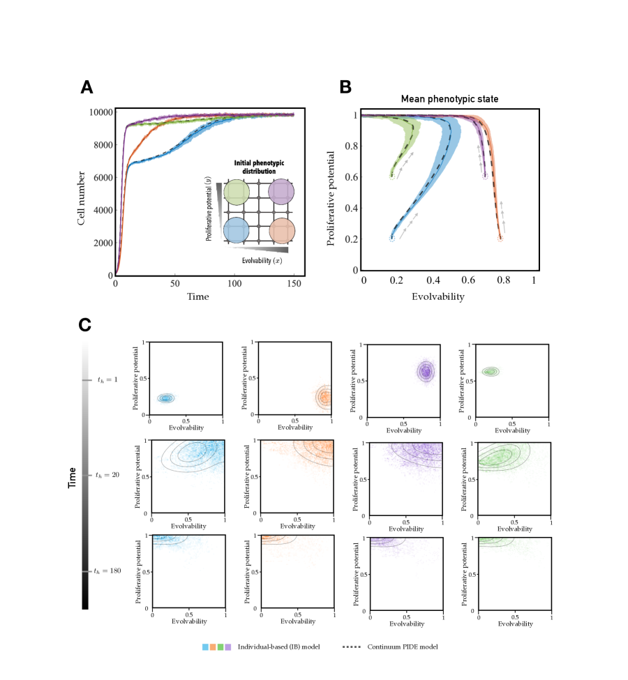
Figure 2: How the initial phenotypic composition affects the evolutionary dynamics A Dynamics of the cell number, results are shown for $t_{h}\in[0,150]$. B Dynamics of the mean phenotypic state for $t_{h}\in[0,150]$. C Phenotypic distribution of the cell population at three different time points ($t_{h}=$ 1, $t_{h}=$ 20, and $t_{h}=$ 150 iterations) for each initial scenario considered. Solid, coloured lines display the results of numerical simulations of the IB model while dashed, black lines display the results of numerical simulations of the continuum model, when evolvability does not imply a fitness cost (i.e. $\alpha=0$), for different values of the initial mean levels of evolvability and proliferative potential – i.e. $(\bar{x}^{0},\bar{y}^{0})=(0.2,0.2)$ (blue lines), $(\bar{x}^{0},\bar{y}^{0})=(0.2,0.6)$ (green lines), $(\bar{x}^{0},\bar{y}^{0})=(0.8,0.2)$ (orange lines), and $(\bar{x}^{0},\bar{y}^{0})=(0.7,0.6)$ (purple lines). The results from the IB model correspond to the average over 20 simulations and the related standard deviation is displayed by the coloured areas surrounding the curves. Numerical simulations of the IB model were carried out using the initial phenotypic distribution defined via Eq. (14) and the parameter values listed in Table 1 with $\alpha=0$ and $\eta=0.5$. Details of numerical simulations of the continuum model are provided in Appendix A2.

3.2 How the strength of natural selection on the proliferative potential affects the evolutionary dynamics

The parameter $\eta$ in Eq. (5) denotes the selection gradient and thus it is a proxy for the strength of selection acting on the cell population. After computing the evolutionary trajectories that arise during the adaptation of cell populations with different initial phenotypic distributions, now we focus on the scenario where the cell population has low initial levels of both evolvability and proliferative potential, and we evaluate how different values of selection strength affect the evolutionary dynamics of the cell population.

The simulation results in Figure 3 illustrate how the strength of natural selection on the proliferative potential (i.e. the value of the selection gradient $\eta$) affects the evolutionary dynamics of the cell population when evolvability does not imply a fitness cost (i.e. when $\alpha=0$). These results demonstrate that the larger the value of the selection gradient $\eta$, the faster both the convergence of the mean level of proliferative potential to the maximum value $1$ and the convergence of the mean level of evolvability to the minimum value $0$. These results also indicate that in scenarios under which the mean level of evolvability undergoes transient growth as discussed in Section 3.1, larger values of the selection gradient $\eta$ cause the mean level of evolvability of the cell population to attain larger values in the transient. For all values of $\eta$ considered here, the phenotype distribution of the cells remains unimodal and the size of the cell population saturates asymptotically to a positive value (results not displayed).

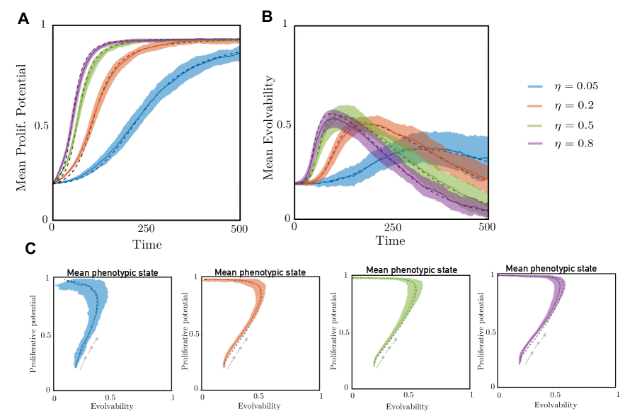
Figure 3: How the strength of natural selection on the proliferative potential affects the evolutionary dynamics. A Dynamics of the mean level of proliferative potential, results are shown for $t_{h}\in[0,500]$. B Dynamics of the mean level of evolvability. C Dynamics of the mean phenotypic state. Solid, coloured lines display the results of numerical simulations of the IB model while dashed, black lines display the results of numerical simulations of the continuum model, when evolvability does not imply a fitness cost (i.e. $\alpha=0$), for different values of the selection gradient $\eta$ – i.e. $\eta=0.05$ (blue lines), $\eta=0.2$ (orange lines), $\eta=0.5$ (green lines) and $\eta=0.8$ (purple lines). The results from the IB model correspond to the average over 20 simulations and the related standard deviation is displayed by the coloured areas surrounding the curves. Numerical simulations of the IB model were carried out using the initial phenotypic distribution defined via Eq. (14) and the parameter values listed in Table 1 with $\alpha=0$ and $(\bar{x}^{0},\bar{y}^{0})=(0.2,0.2)$. Details of numerical simulations of the continuum model are provided in Appendix A2.

3.3 How the fitness cost of evolvability affects the evolutionary dynamics

Evolvability may impair cellular robustness, thereby threatening cell viability [56]. Hence, we now consider how the evolutionary dynamics of the cell would be affected if evolvability implied a fitness cost. In the context of the model, such a trade-off can be easily implemented by increasing the value of the parameter $\alpha$ in Eq. (5).

The simulation results in Figure 4 show how the evolutionary dynamics of the cell population change when there is a fitness cost associated with evolvability (i.e. when $\alpha>0$). These results demonstrate that larger values of the fitness cost of evolvability $\alpha$: promote a faster convergence of the mean level of evolvability to the minimum value $0$ (cf. Figure 4B and Figure 4C); lead to a slower convergence of the mean level of proliferative potential to the maximum value $1$ (cf. Figure 4A and Figure 4C); and hinder possible transient growth of the mean level of evolvability (cf. Figure 4B and Figure 4C). The cell phenotype distribution remains unimodal and the size of the cell population saturates at a positive asymptotic value for all values of $\alpha$ considered here (results not shown).

As an aside, we observe a mismatch in the dynamics of the proliferative potential between the results of the simulations with the IB model and the numerical results of the PIDE model (Figure 4C). This is explained by the small cell number attained by the simulations with the IB model, compared to the numerical results of the PIDE model. Since a higher cost of evolvability means a smaller division probability, it will take more time for cells in the IB model to reach the maximum value of proliferative potential (compared to the PIDE model). In such circumstances stochastic effects, not captured by the deterministic PIDE model, play a more prominent role. Hence, the cell number grows slowly and this is the reason why the mismatch is larger for greater fitness costs of evolvability.

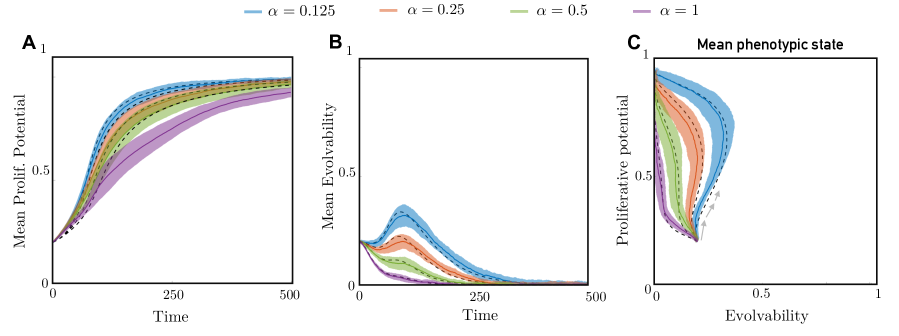
Figure 4: How the fitness cost of evolvability affects the evolutionary dynamics. A Dynamics of the mean level of proliferative potential, results are shown for $t_{h}\in[0,500]$. B Dynamics of the mean level of evolvability. C Dynamics of the mean phenotypic state. Solid, coloured lines display the results of numerical simulations of the IB model while dashed, black lines display the results of numerical simulations of the continuum model, for different values of the fitness cost of evolvability $\alpha$ – i.e. $\alpha=0.125$ (blue line), $\alpha=0.25$ (orange line), $\alpha=0.5$ (green line) and $\alpha=1$ (purple line). The results from the IB model correspond to the average over 20 simulations and the related standard deviation is displayed by the coloured areas surrounding the curves. Numerical simulations of the IB model were carried out using the initial phenotypic distribution defined via Eq. (14) and the parameter values listed in Table 1 with $\eta=0.5$ and $(\bar{x}^{0},\bar{y}^{0})=(0.2,0.2)$. Details of numerical simulations of the continuum model are provided in Appendix A2.

3.4 How the interplay between the strength of natural selection on the proliferative potential and the fitness cost of evolvability affects the evolutionary dynamics.

We now investigate how the interplay between the strength of natural selection on the proliferative potential and the fitness cost of evolvability affect the evolutionary dynamics of the cell population. Since the division rate of a cell is influenced by both $\alpha$ and $\eta$ (cf. Eq. (5)), taking different combinations of these parameters defines different fitness landscapes, whose steepness will determine the ease with which a population can traverse them. Hence, we study the evolutionary dynamics of the cell population subject to different combinations of $\alpha$ and $\eta$, to define fitness landscapes with varying strength of selection and fitness cost of evolvability.

The simulation results in Figures 5 and 6 complement the results in Figures 3 and 4 by showing the impact that the interplay between the strength of natural selection on the proliferative potential and the fitness cost of evolvability may have on the evolutionary dynamics of the cell population. These results demonstrate that large values of the selection gradient $\eta$ and the fitness cost of evolvability $\alpha$ can cause extinction of cell populations when the mean level of evolvability is initially high and the mean level of proliferative potential is initially low (cf. Figures 5C and 5D). This is due to the fact that sufficiently large values of these evolutionary parameters can shape the phenotypic landscape of cell populations in such a way that regions of the landscape corresponding to high levels of evolvability and low levels of proliferative potential are characterised by a negative fitness, i.e. larger values of $\eta$ and $\alpha$ may lead the model function $\rho(x,y)$ to attain negative values for $(x,y)$ sufficiently close to $(1,0)$, thus causing the cell population to suffer a sharp drop in its size if the initial mean phenotypic state lies in these regions (cf. Figures 6C and 6D). This can create the conditions for demographic stochasticity to come into play and drive the cell population to extinction (cf. Figures 5C and 5D). Note that, when this happens, the match between the IB model and the continuum model given by the PIDE (11) deteriorates, since the latter is not capable of capturing population extinction phenomena that are caused by stochastic effects associated with small cell numbers.

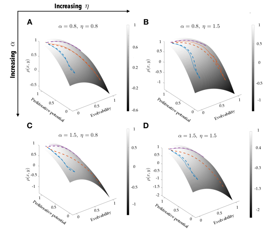
Figure 5: How the interplay between the strength of natural selection on the proliferative potential and the fitness cost of evolvability affects the evolutionary dynamics. A-D Dynamics of the mean phenotypic state. Results are shown for $t_{h}\in[0,500]$. Solid, coloured lines display the results of numerical simulations of the IB model while dashed, coloured lines display the results of numerical simulations of the continuum model, for different values of the selection gradient $\eta$ and the fitness cost of evolvability $\alpha$: $\eta=0.8$ and $\alpha=0.8$ (panel A), $\eta=1.5$ and $\alpha=0.8$ (panel B), $\eta=0.8$ and $\alpha=1.5$ (panel C), and $\eta=1.5$ and $\alpha=1.5$ (panel D), under various scenarios corresponding to different values of the initial mean levels of evolvability and proliferative potential – i.e. $(\bar{x}^{0},\bar{y}^{0})=(0.2,0.2)$ (blue lines), $(\bar{x}^{0},\bar{y}^{0})=(0.8,0.2)$ (orange lines) and $(\bar{x}^{0},\bar{y}^{0})=(0.8,0.8)$ (purple lines). The results from each of 10 simulations of the IB model are displayed. Numerical simulations of the IB model were carried out using the initial phenotypic distribution defined via Eq. (14) and the parameter values listed in Table 1. Details of numerical simulations of the continuum model are provided in Appendix A2.

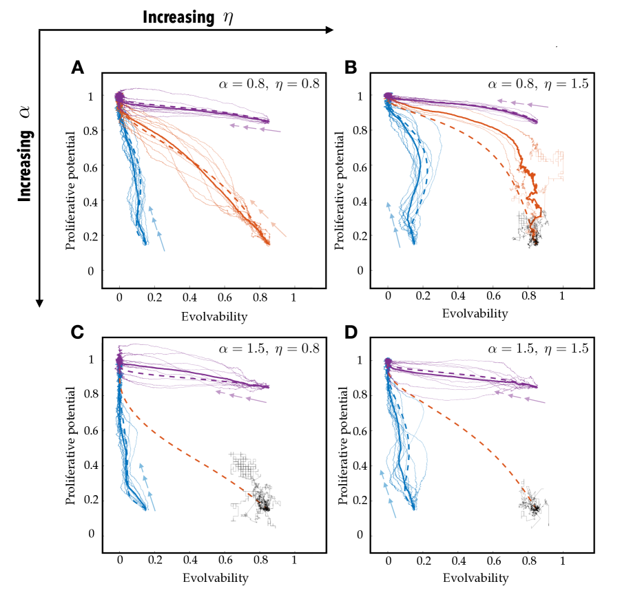
Figure 6: How the interplay between the strength of natural selection on the proliferative potential and the fitness cost of evolvability affects evolutionary dynamics. A-D Dynamics of the mean phenotypic state superimposed onto the phenotypic fitness landscape of the cell population. Results shown for $t_{h}\in[0,500]$. Solid, coloured lines display the results of numerical simulations of the IB model while broken, coloured lines display the results of numerical simulations of the continuum model, for different values of the selection gradient $\eta$ and the fitness cost of evolvability $\alpha$ – i.e. $\eta=0.8$ and $\alpha=0.8$ (panel A), $\eta=1.5$ and $\alpha=0.8$ (panel B), $\eta=0.8$ and $\alpha=1.5$ (panel C), and $\eta=1.5$ and $\alpha=1.5$ (panel D), under various scenarios corresponding to different values of the initial mean levels of evolvability and proliferative potential – i.e. $(\bar{x}^{0},\bar{y}^{0})=(0.2,0.2)$ (blue lines), $(\bar{x}^{0},\bar{y}^{0})=(0.8,0.2)$ (orange lines), and $(\bar{x}^{0},\bar{y}^{0})=(0.8,0.8)$ (purple lines). The grey-scale surfaces are the plots of the function $\rho(x,y)$ defined via Eq. (5) for the different values of $\eta$ and $\alpha$ considered. The results from the IB model correspond to the average over the results of 10 simulations displayed in Figure 5. Solid, coloured lines are not displayed in the cases where the cell population goes extinct in each of the 10 simulations, with the results of simulations in which the cell population goes extinct being highlighted in black. Numerical simulations of the IB model were carried out using the initial phenotypic distribution defined via Eq. (14) and the parameter values listed in Table 1. Details of numerical simulations of the continuum model are provided in Appendix A2.

4 Discussion and conclusions

This theoretical study sheds light on the impact of evolvability on the evolutionary dynamics of phenotypically-structured cell populations. As a natural extension of other works in the field [14, 39, 40, 42, 57], in this paper we consider heritable phenotypic variation and adaptive plasticity that are condensed in evolvability as a cellular trait also subject to evolution [11]. The definition of evolvability that we embrace in this work lies between those of the heritability and evolvability (sensu Wagner) concepts as defined in [12]. At a large evolutionary scale, evolvability could also be termed innovation, generating major phenotypic (morphological, behavioural or physiological) breakthroughs [12, 58]. This last connotation of evolvability strays from the definition considered in this paper.

Both phenotypic plasticity and evolvability are abstract concepts, and delimiting their exact biological influences can be challenging. Nevertheless, it is well-established that they play pivotal roles in the normal functioning of biological systems at various scales, and their significance is intensified under harsh environments such as tumour development [59] or perturbated ecosystems [60, 61, 62]. This interplay can be understood as the intricate interaction amongst various biological phenomena. At a cellular level, these phenomena include biological stochasticity, genetic and epigenetic diversity, genome and protein stability. Considering a broader scale, ecological factors like niche partitioning, species interactions, and natural disturbances are also fundamental.

Evolvability is considered to be a quantitative cell trait in our models, modulating the ability of a cell to change its proliferative potential [63]. Similar to other phenotypic traits, it is susceptible to spontaneous stochastic alterations in each cell, affecting its adaptive potential. Our way of implementing evolvability is subject to certain assumptions. Due to the lack of experimental data, the interaction between proliferation rate and evolvability potential remains unknown and we approached this relationship from a qualitative point of view based on already known biological insights. However, our modelling platform is flexible enough to be tuned as soon as this data become available. Such a biological assumption is based on the assertion that greater adaptability correlates with increased species success, and is purposed as a first step in the study of increasingly complex mathematical models of evolutionary dynamics that include adaptive plasticity.

As a starting point, we studied whether the outcome of the system evolution could be dependent on the initial phenotypic composition of the population. We observed an asymptotic convergence of the simulations to the maximum proliferative potential - lowest evolvability phenotype regardless of the initial condition in an undisturbed environment. Extremely robust DNA repair mechanisms to preserve genome stability [64], intraspecific mutation rate limitations [65, 66, 67, 68], and catabolic convergence and protein stability [69] reflect, to some extent, that these low values of evolvability are positively selected in undisturbed environments and ensure balance and homeostasis at all levels of organisation. However, in our analysis of the results at intermediate time points under various initial conditions in our models, we have observed that cells with a higher degree of evolvability appear to gain a competitive advantage during the initial stages of evolutionary dynamics. This advantageous trait enables them to navigate the phenotypic landscape more swiftly, thereby expediting the process of adaptation. These adaptive dynamics occur through a two-step process, where cells with elevated evolvability are favoured in the short term, while cells exhibiting high proliferative potential and lower evolvability are favoured in the long term (canalisation) [70, 71].

It is essential to recognize that the origins of variation in fitness and adaptive plasticity differ depending on the physical and temporal scale and the specific outcome under consideration. However, the fundamental principles underlying phenomena as different as ecosystem regulation (occurring on large physical and temporal scales) and tumour development (operating over a lifetime and involving organism-level physical dimensions) seem more alike than one might anticipate. At an ecosystemic and evolutionary scale, biodiversity hotspots and adaptive radiation represent high evolvable scenarios, respectively. Through an ecosystemic lens, biodiversity hotspots are biomes with a high net diversification rate [72, 73, 74] originated by a variety of factors including geographical isolation, geological activity or recent climate change. Through an evolutionary lens, adaptive radiation comprises a rapid diversification of a lineage (common ancestor) due to emergence of an ecological opportunity: in other words, newly available ecological niches such as the radiation of the basal mammalian spread [75]. Adaptive radiation is usually followed by a decline phase in diversity which is linked to the continuous adaptation of resident niche specialists [76]. These dynamics relate the results of our population-level models with the less-evolvable more-proliferative phenotype succeeding in the long term, and that evolvability levels are not constant in time. Changes in evolvability are included in our models through the parameter $\omega$.

At a cellular or tissue scale we can also refer to many sources of diversity beyond DNA mutations, even though they are a key mechanism for generating variation. It is widely known that nature creates phenotypic heterogeneity through mechanisms that are not strictly related to DNA mutations. These complementary sources of variation include stochastic gene expression [24, 25, 27, 28, 29], errors in protein synthesis and protein promiscuity [6, 11, 77, 78]. These processes are exacerbated in cancer and allow isogenic populations to evolve and adapt on a short timescale, providing them with the raw material for natural selection to act upon. DNA changes, chromosomal rearrangements and epigenetic modifications can also act as fixation tools for long-term non-genetic phenotypic variation [79]. This phenotypic variation may lead to tiny changes on the proliferative potential (or cell fitness) that we include in our model through the function $\mu(x)$. As previously stated, population variation plays a pivotal role in the operation of natural selection. In our models, it initiates the exploration of the phenotypic landscape.

The results in Figure 2 indicate that phenotypic variants with high proliferative potential and low evolvability are ultimately selected in the cell population, even if evolvability does not imply a fitness cost. When there is no fitness cost associated with evolvability and the initial mean level of evolvability of the cell population is sufficiently low, phenotypic variants with a relatively high evolvability level may have a temporary competitive advantage over the others on intermediate time scales. However, as soon as the mean level of proliferative potential of the cell population becomes sufficiently high, variants with high evolvability are outcompeted by lower evolvability variants. As a result, this high-evolvable phenotype is outcompeted by the phenotype with superior fitness, characterised by a higher proliferative potential.

The influence of selection strength on proliferative potential was also studied, showing that the greater its intensity, the greater the competitive advantage of cells with high evolvability (during the early stages of selection). The results in Figure 3 indicate that, when evolvability does not imply a fitness cost, a stronger selective pressure on the proliferative potential speeds up the selective sweep underlying the fixation of fast-dividing phenotypic variants and it catalyses the selection of phenotypic variants with low evolvability on the long time scale. This scenario also promotes a short-term selection of phenotypic variants with higher evolvability at intermediate time scales, allowing the cells to traverse the phenotypic landscape faster and therefore fixing a high-proliferative low-evolvable average phenotype earlier in time. Thus, stronger selection strength favours or accelerates adaptation, as each jump in the direction of the optimal proliferative potential receives a greater reward. Under challenging environments, increased adaptive plasticity seems to be selected in the short-term in our simulation results, resembling what happens in other natural contexts including adaptive radiation and the onset of therapy resistance. These dynamics mirror the negative epistasis phenomenon observed in numerous fitness landscapes. In this scenario, as a population becomes better adapted to its environment, the success of an advantageous mutation within that population becomes increasingly challenging. This has been reported in asexual E. coli populations [80] although average fitness, i.e. growth rate, continues to increase in time. Other authors reported that this decrease in adaptability is best explained by the reduction of beneficial changes available in the phenotypic space in the same species [81]. The asexual self-cloning division pattern of tumour cells could also reproduce this phenomenon in cancer [82, 83].

Another fact worth noting is that high evolvability may not be free of charge for the cell. In the aforementioned discussion we have ignored the deleterious effects of being evolvable and thus compromising the integrity of fundamental cellular mechanisms. A high level of phenotypic plasticity might compromise cell viability and ultimately phenotypic survival [14]. Hence, it is feasible to assume that evolvability implies a fitness cost. The results in Figure 4 incorporate this phenomenon by considering increasing fitness costs for evolvability (i.e. increasing values of the model parameter $\alpha$). These numerical results support the conclusion that a higher fitness cost of evolvability may cause faster selection of phenotypic variants with low evolvability, thus slowing down the selective sweep that underlies the fixation of fast-dividing phenotypic variants. Although the limits of plasticity have not been studied in as much depth as the benefits of maintaining phenotypic diversity, they have been shown to have evolutionary consequences [48]. Robustness of the network of cellular processes is provided by genetic mutations, gene duplications, and redundancy of fundamental metabolic pathways or structural cell functions (chaperones, protein stability and more [11, 49, 84]). Subsequently, cells with high evolvability may suffer from developmental instability and decreased robustness [85]. A high evolvability may also give rise to other biological phenomena such as pleiotropy [56, 86] or epistasis [87], since plasticity-associated genes could be also modifying the expression of other unrelated genes. The inclusion of a cost of evolvability in the model hinders the selection of cells with higher evolvability during the early stages of evolutionary dynamics.

However, in the context of cancer, tumour cells appear to have compensated for possible negative effects of higher evolvability through the parallel selection of alternative multiple metabolic and genetic mechanisms that enhance cell viability, such as cell redundancy, copy number variation, and degeneration. Therefore, tumour cells may be better able to inhabit this low-intermediate evolvability fitness cost window, leaving room for exploratory behaviour and leading to the known increased phenotypic heterogeneity observed in cancer [88, 89, 90, 91].

Finally, we explored the impact of different phenotypic landscapes on the evolutionary dynamics of cell populations when both the strength of selection and the cost of evolvability come into play. In the most restrictive cases, where high selection strength and high cost of evolvability coincide, the phenotypic landscape can be so harsh that we can create the conditions for the extinction of certain populations (depending on their initial phenotypic distribution) due to demographic stochasticity. Such extinctions can only be observed using the discrete model, given its stochastic nature; in the continuum model, the population never goes extinct unless a population that reaches a size smaller than 1 is considered to be extinct, such as in [14]. This disagreement between the two models shows the importance of both paradigms when studying the evolutionary dynamics of cell populations: deterministic continuum models allow us to study the average behaviour of large populations, while stochastic discrete models allow us to observe rare phenomena that can be magnified at small population sizes. In future work, it would be insightful to perform a mathematical analysis of the continuum model used in this work, to explore the qualitative and quantitative properties of the solutions of this model, and to study the asymptotic behaviour of the cell populations described by it, evaluating the influence of evolvability in the evolutionary dynamics.

The findings presented in Figures 5 and 6 suggest that in more challenging environments, where stronger natural selection acts upon proliferative potential, a substantial fitness cost associated with evolvability could potentially contribute to the extinction of cell populations. These cell populations would be primarily composed of slow-dividing, less fit phenotypic variants possessing a high degree of evolvability. The error catastrophe [92] in viruses caused by mutation rates above a critical value is an example of such a situation, where a rapidly mutating viral genome loses the ability to preserve its integrity [93]. The interaction between elevated values of $\alpha$ and $\eta$ (cf. Eq. (5)) in our models appears to drive the population below the Allee threshold. However, it is crucial to acknowledge that the persistence of a population is also contingent upon genetic and phenotypic variance, and the facilitation of bounded adaptive evolution (evolvability) can promote the successful establishment of a population [63, 94].

In our current model, we have focused on a static phenotypic landscape. However, exploring the impact of evolving extrinsic selection pressures – such as antibiotic, cytotoxic, or chemotherapeutic treatments, contingent on cell type – on the evolutionary dynamics of populations undergoing changes in evolvability is a critical aspect for further investigation. These considerations, including therapies affecting cell stemness or inducing chromosomal instability, may significantly influence the evolvability of cancer cells [95, 96]. Extending our model to encompass various extrinsic pressures, such as conventional cytotoxic therapies affecting highly proliferative cells in cancer, but also potential epigenetic drugs targeting highly evolvable cells, could provide valuable insights that could support the development of innovative therapeutic approaches against cancer.

5 Funding

This work was supported by the Spanish Ministerio de Ciencia e Innovación, the European Union NextGenerationEU/PRTR, MCIN/AEI/10.13039/501100011033 (grant numbers PID2022-142341OB-I00), Junta de Comunidades de Castilla-La Mancha (grant SBPLY/21/180501/ 000145) and by University of Castilla-La Mancha/European Regional Development Fund (FEDER; grant number 2022-GRIN-34405). JJS acknowledges funding support by Universidad de Castilla-La Mancha (grant number 2020-PREDUCLM-15634) and would like to thank also the Mathematical Institute (University of Oxford), and the Dipartimento di Scienze Matematiche (DISMA, Politecnico di Torino), for their support and hospitality during the development of this work. COS thanks the Spanish League Against Cancer (AECC) for their support (grant number 2019-PRED-28372). PKM would like to thank the Isaac Newton Institute for Mathematical Sciences, Cambridge, for support and hospitality during the programme Mathematics of Movement where work on this paper was undertaken. This work was supported by EPSRC grant no EP/R014604/1. TL gratefully acknowledges support from the Italian Ministry of University and Research (MUR) through the grant PRIN 2020 project (No. 2020JLWP23) “Integrated Mathematical Approaches to Socio-Epidemiological Dynamics” (CUP: E15F21005420006) and the grant PRIN2022-PNRR project (No. P2022Z7ZAJ) “A Unitary Mathematical Framework for Modelling Muscular Dystrophies” (CUP: E53D23018070001). TL gratefully acknowledges also support from the Istituto Nazionale di Alta Matematica (INdAM) and the Gruppo Nazionale per la Fisica Matematica (GNFM).

APPENDIX

A1 Formal derivation of the continuum model

In the case where, between time-steps $h$ and $h+1$, each cell in phenotypic state $(y_{i},x_{j})\in(0,1)\times(0,1)$ undergoes phenotypic changes and divides or dies according to the rules described in Section 2.1, the principle of mass balance gives the following difference equation

$$n^{h+1}_{i,j}=\left(1+\Delta tR(y_{i},x_{j},N^{h})\right)\\ \times\left\{\frac{\mu(x_{j})}{2}\left(n^{h}_{i-1,j}+n^{h}_{i+1,j}\right)+\frac{\omega}{2}\left(n^{h}_{i,j-1}+n^{h}_{i,j+1}\right)+\left[1-\left(\omega+\mu(x_{j})\right)\right]n^{h}_{i,j}\right\}.$$ (A1)

Using the fact that for $\Delta t$, $\Delta y$ and $\Delta x$ sufficiently small, the following relations hold

$$t_{h}\approx t,\hskip 14.22636ptt_{h+1}\approx t+\Delta t$$

$$y_{i}\approx y,\hskip 14.22636pty_{i\pm 1}\approx y\pm\Delta y$$

$$x_{j}\approx x,\hskip 14.22636ptx_{j\pm 1}\approx x\pm\Delta x$$

$$n^{h}_{i,j}\approx n(t,y,x),\hskip 11.38109ptn^{h+1}_{i,j}\approx n(t+\Delta t,y,x)$$

$$n^{h}_{i\pm 1,j}\approx n(t,y\pm\Delta y,x)$$

$$n^{h}_{i,j\pm 1}\approx n(t,y,x\pm\Delta x)$$

$$N^{h}\approx N(t):=\int_{0}^{1}\int_{0}^{1}n(t,y,x)\;\textrm{d}y\;\textrm{d}x,$$

Eq. (A1) can be formally rewritten in the approximate form

$$n(t+\Delta t,y,x)=\left(1+\Delta tR(y,x,N)\right)\left\{\frac{\mu(x)}{2}\left(n(t,y-\Delta y,x)+n(t,y+\Delta y,x)\right)\right.\\ \left.+\frac{\omega}{2}\left(n(t,y,x-\Delta x)+n(t,y,x+\Delta x)\right)+\left[1-\left(\omega+\mu(x)\right)\right]n(t,y,x)\right\}.$$ (A2)

If the function $n(t,y,x)$ is twice continuously differentiable with respect to the variables $y$ and $x$, then for $\Delta y$ and $\Delta x$ sufficiently small, we can use the Taylor expansions

$$n(t,y\pm\Delta y,x)=n(t,y,x)\pm\Delta y\partial_{y}n(t,y,x)+\frac{\left(\Delta y\right)^{2}}{2}\partial_{yy}^{2}n(t,y,x)+o(\left(\Delta y\right)^{2})$$

and

$$n(t,y,x\pm\Delta x)=n(t,y,x)\pm\Delta x\partial_{x}n(t,y,x)+\frac{\left(\Delta x\right)^{2}}{2}\partial_{xx}^{2}n(t,y,x)+o(\left(\Delta x\right)^{2})\,.$$

Substituting these Taylor expansions into Eq. (A2), after a little algebra, we obtain the following equation

$$\dfrac{n(t+\Delta t,y,x)-n(t,y,x)}{\Delta t}=R(y,x,N)\,n(t,y,x)\\ +\left(\frac{\left(\Delta x\right)^{2}\omega}{2\Delta t}\partial_{xx}^{2}n(t,y,x)+\frac{\left(\Delta y\right)^{2}\mu(x)}{2\Delta t}\partial_{yy}^{2}n(t,y,x)\right)+h.o.t.\,.$$ (A3)

If the function $n(t,y,x)$ is also continuously differentiable with respect to the variable $t$, letting $\Delta t\rightarrow 0$, $\Delta y\rightarrow 0$ and $\Delta x\rightarrow 0$ in such a way that the conditions given by Eq. (10) are met, from the latter equation we formally obtain the PIDE (11). Finally, zero-Neumann (i.e. no-flux) boundary conditions on the boundary of the square $[0,1]\times[0,1]$ follow from the fact that the attempted phenotypic changes of the cells are aborted if they require moving into a phenotypic state that does not belong to the square $[0,1]\times[0,1]$.

The mean levels of proliferative potential (2) and evolvability (3) defined in Section 2.1 have the following corresponding functions in the continuum counterpart:

$$\bar{y}(t):=\frac{1}{N(t)}\int_{0}^{1}\int_{0}^{1}y\,n(t,y,x)\,\textrm{d}y\,\textrm{d}x,\quad\sigma_{y}(t):=\left(\frac{1}{N(t)}\int_{0}^{1}\int_{0}^{1}y^{2}\,n(t,y,x)\,\textrm{d}y\,\textrm{d}x-\left(\bar{y}(t)\right)^{2}\right)^{1/2}$$ (A4)

and

$$\bar{x}(t):=\frac{1}{N(t)}\int_{0}^{1}\int_{0}^{1}x\,n(t,y,x)\,\textrm{d}x\,\textrm{d}y,\quad\sigma_{x}(t):=\left(\frac{1}{N(t)}\int_{0}^{1}\int_{0}^{1}x^{2}\,n(t,y,x)\,\textrm{d}x\,\textrm{d}y-\left(\bar{x}(t)\right)^{2}\right)^{1/2}.$$ (A5)

A2 Details of numerical simulations of the continuum model

To solve numerically the PIDE (11) subject to no-flux boundary conditions on the boundary of the square $[0,1]\times[0,1]$ and complemented with the continuum analogue of the initial condition defined via Eq. (14), i.e.

$$n(0,y,x)=n^{0}(y,x):=N^{0}\,C\,\exp\left[-\frac{(y-\bar{y}^{0})^{2}}{2(\sigma^{0}_{y})^{2}}-\frac{(x-\bar{x}^{0})^{2}}{2(\sigma^{0}_{x})^{2}}\right]$$

where $C$ is a normalisation constant such that $\displaystyle{\int_{0}^{1}\int_{0}^{1}n^{0}(y,x)\,{\rm d}y\,{\rm d}x=N^{0}}$, we use a uniform discretisation of the interval $(0,1)$ as the computational domain of the independent variables $y$ and $x$, and a uniform discretisation of the interval $(0,t_{f}]$ with $t_{f}=\left\{500,1000\right\}$ as the computational domain of the independent variable $t$. The method for constructing numerical solutions is based on a three-point finite difference explicit scheme for the diffusion terms and an explicit finite difference scheme for the reaction term [97]. The parameter values are chosen to be consistent with those used to carry out numerical simulations of the IB model, which are specified in the main body of the paper.

References

- [1] Charles Darwin. On the origin of species by means of natural selection, or the preservation of favoured races in the struggle for life. London: Murray, 1859.
- [2] David Houle. Comparing evolvability and variability of quantitative traits. Genetics, 130(1):195–204, 1992.
- [3] Michael Lynch, Bruce Walsh, et al. Genetics and analysis of quantitative traits, volume 1. Sinauer Sunderland, MA, 1998.
- [4] Ary A Hoffmann and Juha Merilä. Heritable variation and evolution under favourable and unfavourable conditions. Trends in Ecology & Evolution, 14(3):96–101, 1999.
- [5] Rowan DH Barrett and Dolph Schluter. Adaptation from standing genetic variation. Trends in ecology & evolution, 23(1):38–44, 2008.
- [6] Alex Sigal, Ron Milo, Ariel Cohen, Naama Geva-Zatorsky, Yael Klein, Yuvalal Liron, Nitzan Rosenfeld, Tamar Danon, Natalie Perzov, and Uri Alon. Variability and memory of protein levels in human cells. Nature, 444(7119):643–646, 2006.
- [7] Thomas A Kunkel and Katarzyna Bebenek. Dna replication fidelity. Annual review of biochemistry, 69(1):497–529, 2000.
- [8] Adam Eyre-Walker and Peter D Keightley. The distribution of fitness effects of new mutations. Nature Reviews Genetics, 8(8):610–618, 2007.
- [9] Adam Eyre-Walker. The genomic rate of adaptive evolution. Trends in ecology & evolution, 21(10):569–575, 2006.
- [10] Marc Kirschner and John Gerhart. Evolvability. Proceedings of the National Academy of Sciences, 95(15):8420–8427, 1998.
- [11] Joshua L Payne and Andreas Wagner. The causes of evolvability and their evolution. Nature Reviews Genetics, 20(1):24–38, 2019.
- [12] Massimo Pigliucci. Is evolvability evolvable? Nature Reviews Genetics, 9(1):75–82, 2008.
- [13] Joanna Masel and Meredith V Trotter. Robustness and evolvability. Trends in Genetics, 26(9):406–414, 2010.
- [14] Anuraag Bukkuri, Kenneth J Pienta, Sarah R Amend, Robert H Austin, Emma U Hammarlund, and Joel S Brown. The contribution of evolvability to the eco-evolutionary dynamics of competing species. Ecology and Evolution, 13(10), 2023.
- [15] Dan Cohen. Optimizing reproduction in a randomly varying environment. Journal of Theoretical Biology, 12:119–129, 1966.
- [16] Paul H. Harvey and Linda Partridge. What is bet-hedging? Oxford Surveys in Evolutionary Biology, 4:182–211, 1987.
- [17] Montgomery Slatkin. Hedging one’s evolutionary bets. Nature, 250:704–705, 1974.
- [18] Jana M Riederer, Stefano Tiso, Timo JB van Eldijk, and Franz J Weissing. Capturing the facets of evolvability in a mechanistic framework. Trends in Ecology & Evolution, 37(5):430–439, 2022.
- [19] N Colegrave and Sinéd Collins. Experimental evolution: experimental evolution and evolvability. Heredity, 100(5):464–470, 2008.
- [20] Joshua L Payne and Andreas Wagner. The robustness and evolvability of transcription factor binding sites. Science, 343(6173):875–877, 2014.
- [21] Andreas Wagner. Evolvability-enhancing mutations in the fitness landscapes of an RNA and a protein. Nature Communications, 14(1):3624, 2023.
- [22] Rodrigo S Galhardo, Philip J Hastings, and Susan M Rosenberg. Mutation as a stress response and the regulation of evolvability. Critical reviews in biochemistry and molecular biology, 42(5):399–435, 2007.
- [23] Heather L True, Ilana Berlin, and Susan L Lindquist. Epigenetic regulation of translation reveals hidden genetic variation to produce complex traits. Nature, 431(7005):184–187, 2004.
- [24] William J Blake, Mads Kærn, Charles R Cantor, and James J Collins. Noise in eukaryotic gene expression. Nature, 422(6932):633–637, 2003.
- [25] Michael B Elowitz, Arnold J Levine, Eric D Siggia, and Peter S Swain. Stochastic gene expression in a single cell. Science, 297(5584):1183–1186, 2002.
- [26] D Allan Drummond and Claus O Wilke. The evolutionary consequences of erroneous protein synthesis. Nature Reviews Genetics, 10(10):715–724, 2009.
- [27] Harley H McAdams and Adam Arkin. It’sa noisy business! genetic regulation at the nanomolar scale. Trends in genetics, 15(2):65–69, 1999.
- [28] Jonathan M Raser and Erin K O’shea. Noise in gene expression: origins, consequences, and control. Science, 309(5743):2010–2013, 2005.
- [29] Alvaro Sanchez and Ido Golding. Genetic determinants and cellular constraints in noisy gene expression. Science, 342(6163):1188–1193, 2013.
- [30] Jean‐Pascal Capp. Interplay between genetic, epigenetic, and gene expression variability: Considering complexity in evolvability. Evolutionary Applications, 14(4):893–901, April 2021.
- [31] Michael Tyler Guinn, Yiming Wan, Sarah Levovitz, Dongbo Yang, Marsha R. Rosner, and Gábor Balázsi. Observation and Control of Gene Expression Noise: Barrier Crossing Analogies Between Drug Resistance and Metastasis. Front. Genet., 11:586726, October 2020.
- [32] Zoltán Bódi, Zoltán Farkas, Dmitry Nevozhay, Dorottya Kalapis, Viktória Lázár, Bálint Csörgő, Ákos Nyerges, Béla Szamecz, Gergely Fekete, Balázs Papp, Hugo Araújo, José L. Oliveira, Gabriela Moura, Manuel A. S. Santos, Tamás Székely Jr, Gábor Balázsi, and Csaba Pál. Phenotypic heterogeneity promotes adaptive evolution. PLoS Biol, 15(5):e2000644, May 2017.
- [33] Anton Crombach and Paulien Hogeweg. Evolution of evolvability in gene regulatory networks. PLoS computational biology, 4(7):e1000112, 2008.
- [34] Jeremy Draghi and Gunter P Wagner. The evolutionary dynamics of evolvability in a gene network model. Journal of evolutionary biology, 22(3):599–611, 2009.
- [35] Thomas D Cuypers, Jacob P Rutten, and Paulien Hogeweg. Evolution of evolvability and phenotypic plasticity in virtual cells. BMC evolutionary biology, 17:1–16, 2017.
- [36] Simon J Hickinbotham, Susan Stepney, and Paulien Hogeweg. Nothing in evolution makes sense except in the light of parasitism: evolution of complex replication strategies. Royal Society Open Science, 8(8):210441, 2021.
- [37] Rebecca H Chisholm, Tommaso Lorenzi, and Jean Clairambault. Cell population heterogeneity and evolution towards drug resistance in cancer: biological and mathematical assessment, theoretical treatment optimisation. Biochimica et Biophysica Acta (BBA)-General Subjects, 1860(11):2627–2645, 2016.
- [38] Tommaso Lorenzi, Rebecca H Chisholm, and Jean Clairambault. Tracking the evolution of cancer cell populations through the mathematical lens of phenotype-structured equations. Biology direct, 11(1):1–17, 2016.
- [39] Aleksandra Ardaševa, Robert A. Gatenby, Alexander R. A. Anderson, Helen M. Byrne, Philip K. Maini, and Tommaso Lorenzi. Evolutionary dynamics of competing phenotype-structured populations in periodically fluctuating environments. J. Math. Biol., 80(3):775–807, February 2020.
- [40] Aleksandra Ardaševa, Alexander RA Anderson, Robert A Gatenby, Helen M Byrne, Philip K Maini, and Tommaso Lorenzi. Comparative study between discrete and continuum models for the evolution of competing phenotype-structured cell populations in dynamical environments. Physical Review E, 102(4):042404, 2020.
- [41] Aleksandra Ardaševa, Robert A Gatenby, Alexander RA Anderson, Helen M Byrne, Philip K Maini, and Tommaso Lorenzi. A mathematical dissection of the adaptation of cell populations to fluctuating oxygen levels. Bulletin of Mathematical Biology, 82(6):1–24, 2020.
- [42] Carmen Ortega-Sabater, Gabriel F Calvo, Jelena Dinić, Ana Podolski-Renic, Milica Pesic, and Víctor M Pérez-García. Stochastic fluctuations drive non-genetic evolution of proliferation in clonal cancer cell populations. bioRxiv, pages 2021–06, 2022.
- [43] Mark A Feitelson, Alla Arzumanyan, Rob J Kulathinal, Stacy W Blain, Randall F Holcombe, Jamal Mahajna, Maria Marino, Maria L Martinez-Chantar, Roman Nawroth, Isidro Sanchez-Garcia, et al. Sustained proliferation in cancer: Mechanisms and novel therapeutic targets. Seminars in cancer biology, 35:S25–S54, 2015.
- [44] Li Guo, Yaodong Zhang, Zibo Yin, Yaya Ji, Guowei Yang, Bowen Qian, Sunjing Li, Jun Wang, Tingming Liang, Changxian Li, et al. Screening and identification of genes associated with cell proliferation in cholangiocarcinoma. Aging (Albany NY), 12(3):2626, 2020.
- [45] Torsten O Nielsen, Joel S Parker, Samuel Leung, David Voduc, Mark Ebbert, Tammi Vickery, Sherri R Davies, Jacqueline Snider, Inge J Stijleman, Jerry Reed, et al. A comparison of pam50 intrinsic subtyping with immunohistochemistry and clinical prognostic factors in tamoxifen-treated estrogen receptor–positive breast cancerpam50 in er-positive breast cancer. Clinical cancer research, 16(21):5222–5232, 2010.
- [46] Firoz Ahmed. Integrated network analysis reveals foxm1 and mybl2 as key regulators of cell proliferation in non-small cell lung cancer. Frontiers in oncology, 9:1011, 2019.
- [47] Ron Geller, Sebastian Pechmann, Ashley Acevedo, Raul Andino, and Judith Frydman. Hsp90 shapes protein and rna evolution to balance trade-offs between protein stability and aggregation. Nature communications, 9(1):1781, 2018.
- [48] Thomas J. DeWitt, Andrew Sih, and David Sloan Wilson. Costs and limits of phenotypic plasticity. Trends in Ecology & Evolution, 13(2):77–81, 1998.
- [49] Jesse D Bloom, Zhongyi Lu, David Chen, Alpan Raval, Ophelia S Venturelli, and Frances H Arnold. Evolution favors protein mutational robustness in sufficiently large populations. BMC Biol, 5(1):29, December 2007.
- [50] Amy Brock, Hannah Chang, and Sui Huang. Non-genetic heterogeneity—a mutation-independent driving force for the somatic evolution of tumours. Nature Reviews Genetics, 10(5):336–342, 2009.
- [51] Sui Huang. Genetic and non-genetic instability in tumor progression: link between the fitness landscape and the epigenetic landscape of cancer cells. Cancer and Metastasis Reviews, 32:423–448, 2013.
- [52] F. Bubba, T. Lorenzi, and F. R. Macfarlane. From a discrete model of chemotaxis with volume-filling to a generalized Patlak-Keller-Segel model. Proc. R. Soc. A, 476(2237):20190871, 2020.
- [53] M. A. J. Chaplain, T. Lorenzi, and F.R. Macfarlane. Bridging the gap between individual-based and continuum models of growing cell populations. J. Math. Biol., 80(1):343–371, 2020.
- [54] R. E. A. Stace, T. Stiehl, M. A. J. Chaplain, A. Marciniak-Czochra, and T. Lorenzi. Discrete and continuum phenotype-structured models for the evolution of cancer cell populations under chemotherapy. Math. Mod. Nat. Phen., 15:14, 2020.
- [55] Sean H Rice. Evolutionary theory: mathematical and conceptual foundations. Sinauer Associates Sunderland, MA, 2004.
- [56] George C. Williams. Pleiotropy, natural selection, and the evolution of senescence. Evolution, 11(4):398–411, 1957.
- [57] Fiona R Macfarlane, Xinran Ruan, and Tommaso Lorenzi. Individual-based and continuum models of phenotypically heterogeneous growing cell populations. AIMS Bioengineering, 9(1):68–92, 2022.
- [58] Eörs Szathmáry and John Maynard Smith. The major evolutionary transitions. Nature, 374(6519):227–232, 1995.
- [59] Garrett Jenkinson, Elisabet Pujadas, John Goutsias, and Andrew P Feinberg. Potential energy landscapes identify the information-theoretic nature of the epigenome. Nat Genet, 49(5):719–729, May 2017.
- [60] Aidan M. C. Couzens and G. Prideaux. Rapid pliocene adaptive radiation of modern kangaroos. Science, 362:72 – 75, 2018.
- [61] Young-Jun Choi, Santiago Fontenla, Peter U. Fischer, T. Le, A. Costábile, D. Blair, P. Brindley, J. Tort, M. Cabada, and M. Mitreva. Adaptive radiation of the flukes of the family fasciolidae inferred from genome-wide comparisons of key species. Molecular biology and evolution, 2019.
- [62] D. Pincheira‐Donoso, L. P. Harvey, and M. Ruta. What defines an adaptive radiation? macroevolutionary diversification dynamics of an exceptionally species-rich continental lizard radiation. BMC Evolutionary Biology, 15, 2015.
- [63] Kenneth J Pienta, Emma U Hammarlund, Robert Axelrod, Joel S Brown, and Sarah R Amend. Poly-aneuploid cancer cells promote evolvability, generating lethal cancer. Evolutionary Applications, 13(7):1626–1634, 2020.
- [64] Nimrat Chatterjee and Graham C Walker. Mechanisms of dna damage, repair, and mutagenesis. Environmental and molecular mutagenesis, 58(5):235–263, 2017.
- [65] Henry Lee-Six, Sigurgeir Olafsson, Peter Ellis, Robert J Osborne, Mathijs A Sanders, Luiza Moore, Nikitas Georgakopoulos, Franco Torrente, Ayesha Noorani, Martin Goddard, et al. The landscape of somatic mutation in normal colorectal epithelial cells. Nature, 574(7779):532–537, 2019.
- [66] Luiza Moore, Daniel Leongamornlert, Tim HH Coorens, Mathijs A Sanders, Peter Ellis, Stefan C Dentro, Kevin J Dawson, Tim Butler, Raheleh Rahbari, Thomas J Mitchell, et al. The mutational landscape of normal human endometrial epithelium. Nature, 580(7805):640–646, 2020.
- [67] Alex Cagan, Adrian Baez-Ortega, Natalia Brzozowska, Federico Abascal, Tim HH Coorens, Mathijs A Sanders, Andrew RJ Lawson, Luke MR Harvey, Shriram Bhosle, David Jones, et al. Somatic mutation rates scale with lifespan across mammals. Nature, 604(7906):517–524, 2022.
- [68] Michael Lynch. The lower bound to the evolution of mutation rates. Genome biology and evolution, 3:1107–1118, 2011.
- [69] Konstantin B Zeldovich, Peiqiu Chen, and Eugene I Shakhnovich. Protein stability imposes limits on organism complexity and speed of molecular evolution. Proceedings of the National Academy of Sciences, 104(41):16152–16157, 2007.
- [70] C.H. Waddington. The Strategy of the Genes: A Discussion of Some Aspects of Theoretical Biology. Allen & Unwin, 1957.
- [71] Jin Wang, Kun Zhang, Li Xu, and Erkang Wang. Quantifying the waddington landscape and biological paths for development and differentiation. Proceedings of the National Academy of Sciences, 108(20):8257–8262, 2011.
- [72] Santiago Madriñán, Andrés J Cortés, and James E Richardson. Páramo is the world’s fastest evolving and coolest biodiversity hotspot. Frontiers in genetics, 4:192, 2013.
- [73] C. Orme, R. G. Davies, M. Burgess, F. Eigenbrod, Nicola J Pickup, V. Olson, A. J. Webster, Tzung-Su Ding, P. Rasmussen, R. Ridgely, A. Stattersfield, P. Bennett, T. Blackburn, K. Gaston, and I. Owens. Global hotspots of species richness are not congruent with endemism or threat. Nature, 436:1016–1019, 2005.
- [74] Norman Myers, Russell A Mittermeier, Cristina G Mittermeier, Gustavo AB Da Fonseca, and Jennifer Kent. Biodiversity hotspots for conservation priorities. Nature, 403(6772):853–858, 2000.
- [75] Dolph Schluter. Ecological causes of adaptive radiation. The American Naturalist, 148:S40–S64, 1996.
- [76] Justin R. Meyer, S. Schoustra, J. Lachapelle, and R. Kassen. Overshooting dynamics in a model adaptive radiation. Proceedings of the Royal Society B: Biological Sciences, 278:392 – 398, 2011.
- [77] Dion J Whitehead, Claus O Wilke, David Vernazobres, and Erich Bornberg-Bauer. The look-ahead effect of phenotypic mutations. Biol Direct, 3(1):18, 2008.
- [78] Amir Aharoni, Leonid Gaidukov, Olga Khersonsky, Stephen McQ Gould, Cintia Roodveldt, and Dan S Tawfik. The ’evolvability’ of promiscuous protein functions. Nat Genet, 37(1):73–76, January 2005.
- [79] Stuart A Kauffman. Requierements for evolvability in complex systems: orderly dynamics and frozen components. PhysicaD, 42(1-3):135–152, 1990.
- [80] Michael J Wiser, Noah Ribeck, and Richard E Lenski. Long-term dynamics of adaptation in asexual populations. Science, 342(6164):1364–1367, 2013.
- [81] Andrea Wünsche, Duy M Dinh, Rebecca S Satterwhite, Carolina Diaz Arenas, Daniel M Stoebel, and Tim F Cooper. Diminishing-returns epistasis decreases adaptability along an evolutionary trajectory. Nature ecology & evolution, 1(4):0061, 2017.
- [82] John E Dick. Stem cell concepts renew cancer research. Blood, The Journal of the American Society of Hematology, 112(13):4793–4807, 2008.
- [83] Joris van de Haar, Sander Canisius, K Yu Michael, Emile E Voest, Lodewyk FA Wessels, and Trey Ideker. Identifying epistasis in cancer genomes: a delicate affair. Cell, 177(6):1375–1383, 2019.
- [84] G. J. Szollosi and I. Derenyi. Congruent Evolution of Genetic and Environmental Robustness in Micro-RNA. Molecular Biology and Evolution, 26(4):867–874, January 2009.
- [85] Christian Peter Klingenberg. Phenotypic plasticity, developmental instability, and robustness: The concepts and how they are connected. Frontiers in Ecology and Evolution, 7, 2019.
- [86] Stephanie A. Bien and Ulrike Peters. Moving from one to many: insights from the growing list of pleiotropic cancer risk genes. British Journal of Cancer, 120(12):1087–1089, June 2019.
- [87] Samuel M. Scheiner. Genetics and evolution of phenotypic plasticity. Annual Review of Ecology and Systematics, 24(1):35–68, 1993.
- [88] Jacob Househam, Timon Heide, G. Cresswell, Claire Lynn, I. Spiteri, M. Mossner, C. Kimberley, Calum Gabbutt, E. Lakatos, J. Fernández-Mateos, Bingjie Chen, L. Zapata, C. James, A. Berner, Melissa Schmidt, A. Baker, D. Nichol, Helena Costa, Miriam Mitchinson, M. Jansen, G. Caravagna, D. Shibata, J. Bridgewater, M. Rodríguez-Justo, L. Magnani, A. Sottoriva, and T. Graham. Phenotypic plasticity and genetic control in colorectal cancer evolution. Nature, 611:744 – 753, 2021.
- [89] Cyril Neftel, Julie Laffy, Mariella G Filbin, Toshiro Hara, Marni E Shore, Gilbert J Rahme, Alyssa R Richman, Dana Silverbush, McKenzie L Shaw, Christine M Hebert, et al. An Integrative Model of Cellular States, Plasticity, and Genetics for Glioblastoma. Cell, 178(4):835–849.e21, 2019.
- [90] Piyush B Gupta, Ievgenia Pastushenko, Adam Skibinski, Cedric Blanpain, and Charlotte Kuperwasser. Phenotypic plasticity: driver of cancer initiation, progression, and therapy resistance. Cell stem cell, 24(1):65–78, 2019.
- [91] Saumil Shah, Lisa-Marie Philipp, Stefano Giaimo, Susanne Sebens, Arne Traulsen, and Michael Raatz. Understanding and leveraging phenotypic plasticity during metastasis formation. NPJ Systems Biology and Applications, 9(1):48, 2023.
- [92] Manfred Eigen. Selforganization of matter and the evolution of biological macromolecules. Naturwissenschaften, 58(10):465–523, 1971.
- [93] Nonia Pariente, Saleta Sierra, and Antero Airaksinen. Action of mutagenic agents and antiviral inhibitors on foot-and-mouth disease virus. Virus research, 107(2):183–193, 2005.
- [94] Andrew R Kanarek and Colleen T Webb. Allee effects, adaptive evolution, and invasion success. Evolutionary Applications, 3(2):122–135, 2010.
- [95] Nicholas McGranahan, Rebecca A Burrell, David Endesfelder, Marco R Novelli, and Charles Swanton. Cancer chromosomal instability: therapeutic and diagnostic challenges: ‘exploring aneuploidy: the significance of chromosomal imbalance’review series. EMBO reports, 13(6):528–538, 2012.
- [96] Haiyan Yan, Weiguo Lu, and Fangwei Wang. The cgas-sting pathway: a therapeutic target in chromosomally unstable cancers. Signal Transduction and Targeted Therapy, 8(1):45, 2023.
- [97] Randall J LeVeque. Finite difference methods for ordinary and partial differential equations: steady-state and time-dependent problems. Society for Industrial and Applied Mathematics (SIAM), Philadelphia, 2007.