Spectral properties of the Dirichlet-to-Neumann operator for spheroids

Abstract

We study the spectral properties of the Dirichlet-to-Neumann operator and the related Steklov problem in spheroidal domains ranging from a needle to a disk. An explicit matrix representation of this operator for both interior and exterior problems is derived. We show how the anisotropy of spheroids affects the eigenvalues and eigenfunctions of the operator. As examples of physical applications, we discuss diffusion-controlled reactions on spheroidal partially reactive targets and the statistics of encounters between the diffusing particle and the spheroidal boundary.

I Introduction

The Dirichlet-to-Neumann operator ${\mathcal{M}}$ plays an important role in applied mathematics, physics, and engineering. One of its most known applications is related to electrical impedance tomography, also known as Calderon’s problem [1, 2, 3, 4, 5], in which the electric conductivity in the bulk has to be determined from electric measurements on the boundary. The Dirichlet-to-Neumann operator is also employed as a “building block” for analyzing and solving spectral and scattering problems in complex media via domain decomposition (see [6, 7, 8, 9, 10] and references therein). The eigenfunctions of ${\mathcal{M}}$ often appear as a basis for representing and approximating harmonic functions and related quantities [11, 12, 13, 14, 15]. In chemical physics, diffusion-controlled reactions and other diffusion-mediated surface phenomena can be described by means of the operator ${\mathcal{M}}$ [16, 17, 18, 19]. In particular, the statistics of encounters between a diffusing particle and the confining boundary can be determined via a spectral expansion based on the Dirichlet-to-Neumann operator [20, 21, 22]. Its relations to other first-passage time statistics were also investigated [18, 23].

The spectral properties of the Dirichlet-to-Neumann operator and the related Steklov problem were thoroughly investigated for Euclidean domains and Riemannian manifolds (see the recent book [24] and reviews [25, 26]). We focus here on the most basic setting of an Euclidean domain $\Omega\subset{\mathbb{R}}^{d}$ with a smooth bounded boundary $\partial\Omega$. The Dirichlet-to-Neumann operator ${\mathcal{M}}$ is defined as a map of a function $f\in H^{\frac{1}{2}}(\partial\Omega)$ on the boundary $\partial\Omega$ onto another function $g\in H^{-\frac{1}{2}}(\partial\Omega)$ on that boundary such that $g=(\partial_{n}u)|_{\partial\Omega}={\mathcal{M}}f$, where $\partial_{n}$ is the normal derivative oriented outwards the domain $\Omega$, and $u$ is the unique solution of the Dirichlet boundary value problem:

$$\Delta u=0\quad\textrm{in}~{}\Omega,\qquad u=f\quad\textrm{on}~{}\partial\Omega,$$ (1)

with $\Delta$ being the Laplace operator (here $H^{\pm\frac{1}{2}}(\partial\Omega)$ are appropriate functional spaces, see Ref. [24] for mathematical details and references). In other words, the operator ${\mathcal{M}}$ transforms the Dirichlet boundary condition $u|_{\partial\Omega}=f$ on $\partial\Omega$ into an equivalent Neumann boundary condition $(\partial_{n}u)|_{\partial\Omega}={\mathcal{M}}f$. For instance, if $f$ is a given concentration or temperature profile maintained on $\partial\Omega$, then the Laplace equation describes the steady-state regime of molecular or heat diffusion, and $(\partial_{n}u)|_{\partial\Omega}$ is proportional to the flux density on $\partial\Omega$.

When $\Omega$ is bounded, ${\mathcal{M}}$ is known to be pseudo-differential self-adjoint operator with a discrete spectrum, i.e., there is an infinite countable sequence of eigenpairs $\{\mu_{k},v_{k}\}$ satisfying ${\mathcal{M}}v_{k}=\mu_{k}v_{k}$; the nonnegative eigenvalues $\mu_{k}$ are enumerated by $k=0,1,2,\ldots$ in an increasing order,

$$0\leq\mu_{0}\leq\mu_{1}\leq\ldots\nearrow+\infty,$$ (2)

whereas the associated eigenfunctions $\{v_{k}\}$ form a complete basis in the space $L^{2}(\partial\Omega)$ of square-integrable functions on $\partial\Omega$ [24]. Alternatively, one can search for solutions of the Steklov problem,

$$\Delta V_{k}=0\quad\textrm{in}~{}\Omega,\qquad\partial_{n}V_{k}=\mu_{k}V_{k}\quad\textrm{on}~{}\partial\Omega,$$ (3)

where the Steklov eigenvalues standing in the boundary condition are identical to $\mu_{k}$. This tight relation implies that each Steklov eigenfunction $V_{k}$ can be obtained as a harmonic extension of the eigenfunction $v_{k}$ of ${\mathcal{M}}$.

Despite numerous mathematical studies of spectral properties of the Dirichlet-to-Neumann operator [24], intricate relations between its spectrum and the geometric features of the boundary $\partial\Omega$ are not yet fully understood. The eigenvalues and eigenfunctions of ${\mathcal{M}}$ are known explicitly only in few simple domains such as a ball, a space between concentric spheres, the exterior of a ball, and rectangular cuboids [24, 27]. In particular, the role of the boundary anisotropy remains unclear. The situation is even worse for the exterior problem when $\Omega={\mathbb{R}}^{d}\backslash\Omega_{0}$ is the exterior of a bounded domain $\Omega_{0}$. Even though the domain $\Omega$ is unbounded, its boundary $\partial\Omega$ is bounded that implies again the discrete spectrum of the Dirichlet-to-Neumann operator ${\mathcal{M}}$ [12, 13, 28, 15, 29, 30]. However, the analysis of the exterior problem is more difficult; in particular, the mathematical proofs substantially differ for space dimensions $d=2$ and $d\geq 3$. Relations between spectral properties and the geometric shape of $\partial\Omega$ were much less studied. For instance, to our knowledge, the exterior of a ball is the unique example, for which the eigenvalues and eigenfunctions of ${\mathcal{M}}$ are known explicitly for the exterior problem.

In this paper, we study the spectral properties of the Dirichlet-to-Neumann operator ${\mathcal{M}}$ on prolate and oblate spheroidal surfaces that allow one to model various anisotropic shapes in three dimensions, ranging from a needle to a disk. We focus on the less studied exterior spectral problem (an extension to the interior problem is summarized in Appendix A). By employing the prolate/oblate spheroidal coordinates to represent a general solution of the Laplace equation (1), we obtain a convenient matrix representation of the operator ${\mathcal{M}}$. This matrix can then be truncated and diagonalized numerically to approximate the eigenvalues $\mu_{k}$ and eigenfunctions $v_{k}$ of ${\mathcal{M}}$. This efficient technique allows us to investigate how the spectral properties of the Dirichlet-to-Neumann operator depend on the anisotropy of the boundary, especially in the limits of elongated (needle-like) and flattened (disk-like) spheroids. While similar techniques were applied in the past for solving various boundary value problems in spheroidal domains (see, e.g., [31, 32, 33, 34, 35, 36, 37, 38, 39, 40, 41, 42] and references therein), we are not aware of earlier studies of the spectral properties of the Dirichlet-to-Neumann operator in these domains. Sections II and III are devoted respectively to prolate and oblate spheroidal domains. In Sec. IV, we discuss two applications of these results for understanding diffusion-controlled reactions and the statistics of boundary encounters. Section V summarizes our findings and presents future perspectives.

II Prolate spheroids

In this section, we study the Dirichlet-to-Neumann operator ${\mathcal{M}}$ in the exterior of a prolate spheroid with semi-axes $a\leq b$:

$$\Omega=\biggl{\{}(x,y,z)\in{\mathbb{R}}^{3}~{}:~{}\frac{x^{2}}{a^{2}}+\frac{y^{2}}{a^{2}}+\frac{z^{2}}{b^{2}}>1\biggr{\}}.$$ (4)

In the prolate spheroidal coordinates $(\alpha,\theta,\phi)$,

$$\left(\begin{array}[]{c}x\\ y\\ z\\ \end{array}\right)=a_{E}\left(\begin{array}[]{c}\sinh\alpha\sin\theta\cos\phi\\ \sinh\alpha\sin\theta\sin\phi\\ \cosh\alpha\cos\theta\\ \end{array}\right)\qquad\left\{\begin{array}[]{l}0<\alpha<\infty\\ 0\leq\theta\leq\pi\\ 0\leq\phi<2\pi\\ \end{array}\right\},$$

with $a_{E}=\sqrt{b^{2}-a^{2}}$, the scale factors determining the surface and volume elements, are [43]

$$h_{\alpha} =h_{\theta}=a_{E}\sqrt{\sinh^{2}\alpha+\sin^{2}\theta},$$ (5a)

$$h_{\phi} =a_{E}\sinh\alpha\sin\theta.$$ (5b)

In these coordinates, the domain $\Omega$ is characterized by $\alpha>\alpha_{0}=\tanh^{-1}(a/b)$, while its boundary $\partial\Omega$ is determined by the condition $\alpha=\alpha_{0}$.

Matrix representation

A general solution of the Laplace equation in $\Omega$ reads

$$u(\alpha,\theta,\phi)=\sum\limits_{n=0}^{\infty}\sum\limits_{m=-n}^{n}A_{mn}Q_{n}^{m}(\cosh\alpha)Y_{mn}(\theta,\phi),$$ (6)

where $A_{mn}$ are arbitrary coefficients, $Q_{n}^{m}(z)$ are the associated Legendre functions of the second kind (see Appendix B), and

$$Y_{mn}(\theta,\phi) =a_{mn}P_{n}^{m}(\cos\theta)e^{im\phi},$$ (7)

$$a_{mn} =\sqrt{\frac{2n+1}{4\pi}\,\frac{(n-m)!}{(n+m)!}}$$

are the normalized spherical harmonics, with $P_{n}^{m}(x)$ being the associated Legendre polynomials. The normal derivative reads

$$\left.\frac{\partial u}{\partial n}\right|_{\partial\Omega}=-\left.\frac{1}{h_{\alpha}}\partial_{\alpha}u\right|_{\alpha=\alpha_{0}}$$ (8)

$$=-\sum\limits_{n=0}^{\infty}\sum\limits_{m=-n}^{n}A_{mn}Y_{mn}(\theta,\phi)\frac{\sinh\alpha_{0}\,Q^{{}^{\prime}m}_{n}(\cosh\alpha_{0})}{a_{E}\sqrt{\cosh^{2}\alpha_{0}-\cos^{2}\theta}}\,,$$

where prime denotes the derivative with respect to the argument. In other words, for a square-integrable function $f$ on $\partial\Omega$, decomposed on the complete basis of spherical harmonics,

$$f(\theta,\phi)=\sum\limits_{n=0}^{\infty}\sum\limits_{m=-n}^{n}f_{mn}Y_{mn}(\theta,\phi)$$ (9)

(with coefficients $f_{mn}=A_{mn}Q_{n}^{m}(\cosh\alpha_{0})$), the action of the Dirichlet-to-Neumann operator ${\mathcal{M}}$ is

$$[{\mathcal{M}}f](\theta,\phi)=\sum\limits_{n=0}^{\infty}\sum\limits_{m=-n}^{n}f_{mn}\frac{c_{mn}\,Y_{mn}(\theta,\phi)}{\sqrt{\cosh^{2}\alpha_{0}-\cos^{2}\theta}}\,,$$ (10)

where

$$c_{mn}=-\frac{\sinh\alpha_{0}\,Q^{{}^{\prime}m}_{n}(\cosh\alpha_{0})}{a_{E}Q_{n}^{m}(\cosh\alpha_{0})}\,.$$ (11)

At the same time, the function ${\mathcal{M}}f$ can also be decomposed on the complete basis of $Y_{mn}$. Multiplying Eq. (10) by $Y_{m^{\prime}n^{\prime}}^{*}(\theta,\phi)\sin\theta$ and integrating over $\theta$ and $\phi$, one gets

$$[{\mathcal{M}}f](\theta,\phi)=\sum\limits_{n=0}^{\infty}\sum\limits_{m=-n}^{n}[{\bf M}f]_{mn}Y_{mn}(\theta,\phi),$$ (12)

where the (infinite-dimensional) matrix ${\bf M}$ represents the operator ${\mathcal{M}}$ on the orthonormal basis of spherical harmonics, with

$${\bf M}_{mn,m^{\prime}n^{\prime}}=F_{mn,m^{\prime}n^{\prime}}(\cosh\alpha_{0})\,c_{m^{\prime}n^{\prime}},$$ (13)

where

$$F_{mn,m^{\prime}n^{\prime}}(z) =2\pi\,\delta_{m,m^{\prime}}a_{mn}a_{mn^{\prime}}$$

$$\times\int\limits_{-1}^{1}dx\frac{P_{n}^{m}(x)P_{n^{\prime}}^{m}(x)}{\sqrt{z^{2}-x^{2}}}\,.$$ (14)

We stress that the elements of the matrix ${\bf M}$ are enumerated by double indices $mn$ and $m^{\prime}n^{\prime}$. In practice, we employ the following order:

$$\begin{array}[]{c c c c c c c c c c c}mn:&00&(-1)1&01&11&(-2)2&(-1)2&02&12&22&\ldots\\ \end{array}$$

which is borrowed from the enumeration of spherical harmonics.

The eigenvalues of the matrix ${\bf M}$ coincide with the eigenvalues $\mu_{k}$ of the Dirichlet-to-Neumann operator ${\mathcal{M}}$; in turn, each eigenvector ${\bf V}_{k}$ of ${\bf M}$, satisfying ${\bf M}{\bf V}_{k}=\mu_{k}{\bf V}_{k}$, determines the coefficients in the representation of the associated eigenfunction $v_{k}$ on the basis of spherical harmonics:

$$v_{k}(\theta,\phi)=\sum\limits_{n=0}^{\infty}\sum\limits_{m=-n}^{n}[{\bf V}_{k}]_{mn}Y_{mn}(\theta,\phi).$$ (15)

In Appendix B.3, we check the orthogonality of these eigenfunctions to each other; moreover, they can also be normalized as

$$\bigl{(}v_{k},v_{k^{\prime}}\bigr{)}_{L^{2}(\partial\Omega)}=\int\limits_{\partial\Omega}d{\bf s}\,v_{k}^{*}\,v_{k^{\prime}}$$

$$\quad=\int\limits_{0}^{\pi}d\theta\int\limits_{0}^{2\pi}d\phi\,h_{\theta}\,h_{\phi}\,v_{k}^{*}(\theta,\phi)\,v_{k^{\prime}}(\theta,\phi)=\delta_{k,k^{\prime}}.$$ (16)

Using Eq. (6) for a general solution of the Laplace operator, one easily finds a harmonic extension of the eigenfunction $v_{k}$ into $\Omega$, i.e., the Steklov eigenfunction associated to the eigenvalue $\mu_{k}$:

$$V_{k}(\alpha,\theta,\phi)=\sum\limits_{n=0}^{\infty}\sum\limits_{m=-n}^{n}\frac{Q_{n}^{m}(\cosh\alpha)}{Q_{n}^{m}(\cosh\alpha_{0})}[{\bf V}_{k}]_{mn}Y_{mn}(\theta,\phi).$$ (17)

The asymptotic behavior of $Q_{n}^{m}(z)$ for large $|z|$, $Q_{n}^{m}(z)\propto z^{-n-1}$ implies the expected power-law decay of Steklov eigenfunctions in the leading order as $|\bm{x}|\to\infty$:

$$V_{k}(\alpha,\theta,\phi) \simeq\frac{[{\bf V}_{k}]_{00}}{\sqrt{4\pi}\,Q_{0}(\cosh\alpha_{0})}\,\frac{1}{\cosh\alpha}$$

$$\simeq\frac{[{\bf V}_{k}]_{00}}{\sqrt{4\pi}\,Q_{0}(\cosh\alpha_{0})}\frac{a_{E}}{|\bm{x}|}\propto|\bm{x}|^{-1}.$$ (18)

Classification of eigenfunctions

Since the Dirichlet-to-Neumann operator ${\mathcal{M}}$ does not affect the angle $\phi$, the matrix elements ${\bf M}_{mn,m^{\prime}n^{\prime}}$ are nonzero only when $m=m^{\prime}$. In other words, the action of ${\mathcal{M}}$ onto a function $f(\theta)e^{im\phi}$ does not alter its dependence on $\phi$: ${\mathcal{M}}(f(\theta)e^{im\phi})=g(\theta)e^{im\phi}$. As a consequence, any eigenfunction $v_{k}$ depends on $\phi$ via a factor $e^{im\phi}$ for some integer $m$ (or via a linear combination of $e^{im\phi}$ and $e^{-im\phi}$, see below). This property allows one to classify all eigenfunctions according to their dependence on $\phi$ and thus to enumerate them as $v_{mn}(\theta,\phi)$, in analogy to spherical harmonics $Y_{mn}(\theta,\phi)$. Here the index $m$ determines the dependence of the eigenfunction on $\phi$, $v_{mn}(\theta,\phi)\propto e^{im\phi}$, whereas the nonnegative index $n=|m|,|m|+1,|m|+2,\ldots$ enumerates all such functions so that the associated eigenvalues $\mu_{mn}$ appear in an increasing order (for each fixed $m$):

$$0\leq\mu_{m|m|}\leq\mu_{m(|m|+1)}\leq\ldots$$ (19)

Note that the index $n$ starts from $|m|$ in order to automatically satisfy the conventional restriction $|m|\leq n$, known for spherical harmonics.

An alternative way to look at this classification consists in representing the matrix ${\bf M}$ as

$${\bf M}=\sum\limits_{m=-\infty}^{\infty}{\bf M}_{m},$$ (20)

where the (sub)matrix ${\bf M}_{m}$ is composed of elements ${\bf M}_{mn,mn^{\prime}}$ (and $0$ otherwise). For instance, one has

$${\tiny{\bf M}_{0}=\left(\begin{array}[]{c | c c c | c c c c c | c}{\bf M}_{00,00}&0&0&0&0&0&{\bf M}_{00,02}&0&0&\ldots\\ \hline\cr 0&0&0&0&0&0&0&0&0&\ldots\\ 0&0&{\bf M}_{01,01}&0&0&0&0&0&0&\ldots\\ 0&0&0&0&0&0&0&0&0&\ldots\\ \hline\cr 0&0&0&0&0&0&0&0&0&\ldots\\ 0&0&0&0&0&0&0&0&0&\ldots\\ {\bf M}_{02,00}&0&0&0&0&0&{\bf M}_{02,02}&0&0&\ldots\\ 0&0&0&0&0&0&0&0&0&\ldots\\ 0&0&0&0&0&0&0&0&0&\ldots\\ \hline\cr\ldots&\ldots&\ldots&\ldots&\ldots&\ldots&\ldots&\ldots&\ldots&\ldots\\ \end{array}\right).}$$ (21)

If a vector ${\bf X}$ has the form ${\bf X}_{mn}=\delta_{m,m_{0}}x_{n}$ (i.e., its nonzero elements appear only for $m=m_{0}$), then ${\bf M}_{m}{\bf X}=0$ for all $m\neq m_{0}$. In other words, the space $\ell^{2}$ of all vectors with square-summable elements can be decomposed into an (infinite) direct product of subspaces $\ell^{2}_{m}$ enumerated by $m$ ranging from $-\infty$ to $+\infty$. As a consequence, one can diagonalize separately each matrix ${\bf M}_{m}$ and then combine their eigenvalues $\mu_{mn}$ and eigenvectors ${\bf V}_{mn}$ (enumerated by the index $n=|m|,|m|+1,\ldots$) to construct the eigenvalues and eigenvectors of the matrix ${\bf M}$. We expect that the union of all eigenvalues $\mu_{mn}$ gives all eigenvalues of the matrix ${\bf M}$, i.e., such a decomposition determines the whole spectrum of ${\bf M}$. This statement is elementary in the finite-dimensional case, in particular, for a truncation of the matrix ${\bf M}$ that we will use for numerical computations. We can then rewrite the expansions (15, 17) as

$$v_{mn}(\theta,\phi) =\sum\limits_{n^{\prime}=|m|}^{\infty}[{\bf V}_{mn}]_{mn^{\prime}}Y_{mn^{\prime}}(\theta,\phi),$$ (22a)

$$V_{mn}(\alpha,\theta,\phi) =\sum\limits_{n^{\prime}=|m|}^{\infty}\frac{Q_{n^{\prime}}^{m}(\cosh\alpha)}{Q_{n^{\prime}}^{m}(\cosh\alpha_{0})}[{\bf V}_{mn}]_{mn^{\prime}}Y_{mn^{\prime}}(\theta,\phi).$$ (22b)

We note that the symmetry

$$P_{n}^{m}(-x)=(-1)^{m+n}P_{n}^{m}(x),$$ (23)

implies ${\bf M}_{-m}={\bf M}_{m}$ that allows one to restrict $m$ to be nonnegative. As a consequence, any eigenvalue $\mu_{mn}$ with $m\neq 0$ should be (at least) twice degenerate. This degeneracy implies that any linear combination of $v_{(-m)n}$ and $v_{mn}$ is also an eigenfunction. As a consequence, if the eigenfunctions are constructed by using the decomposition (15) based on the diagonalization of the whole matrix ${\bf M}$ and then classified according to their dependence on $\phi$, each eigenfunction $v_{k}$ may in general exhibit the dependence on $\phi$ as a linear combination of $e^{im\phi}$ and $e^{-im\phi}$. An appropriate rotation by a $2\times 2$ matrix can transform a pair of such eigenfunctions into those that are proportional to $e^{im\phi}$ and $e^{-im\phi}$. However, this step is not needed in practice, as we will diagonalize the matrices ${\bf M}_{m}$ to produce directly the required dependence on $\phi$.

In the following, we use interchangeably both notations $\mu_{k},v_{k}$ and $\mu_{mn},v_{mn}$ for eigenvalues and eigenfunctions. We recall that the single-index enumeration relies on the global ordering of all eigenvalues $\mu_{k}$ in Eq. (2). In turn, the double-index enumeration is based on the symmetries of eigenfunctions, namely, on their dependence on $\phi$ via $e^{im\phi}$, whereas the second index $n$ employs the ordering of $\mu_{mn}$ for each $m$ in Eq. (19).

Limit of a sphere

In the limit $a\to b$, the prolate spheroid approaches the sphere of radius $b$. In this limit, one has $a_{E}\to 0$ and $\alpha_{0}\to\infty$ such that $a_{E}\cosh\alpha_{0}=b$ remains constant. As a consequence, the coefficients in Eq. (11) diverge as $c_{mn}\approx\tfrac{n+1}{b}\,\sinh\alpha_{0}$, whereas the matrix elements in Eq. (14) behave in the leading order as $F_{mn,m^{\prime}n^{\prime}}\approx\delta_{n,n^{\prime}}\delta_{m,m^{\prime}}/\cosh\alpha_{0}$, implying that ${\bf M}_{mn,m^{\prime}n^{\prime}}\to\tfrac{n+1}{b}\delta_{n,n^{\prime}}\delta_{m,m^{\prime}}$. The diagonal structure of this matrix yields

$$\mu_{mn}=\frac{n+1}{b}\,,\qquad v_{mn}=\frac{1}{b}\,Y_{mn}(\theta,\phi).$$ (24)

We retrieve therefore the well-known eigenvalues and eigenfunctions of the Dirichlet-to-Neumann operator for the exterior of a sphere. Note that the eigenvalues do not depend on $m$; moreover, since $m$ ranges from $-n$ to $n$, the degeneracy of the eigenvalue $\mu_{mn}$ is $2n+1$, as expected for a sphere due to its rotational symmetry. As illustrated below, the anisotropy of spheroids breaks this symmetry and reduces the degeneracy of eigenvalues.

Numerical implementation

For a practical implementation, infinite-dimensional matrices have to be truncated to a finite size. In a basic setup, one can choose the truncation order $n_{\rm max}$ to keep $n=0,1,2,\ldots,n_{\rm max}$, and then construct the truncated matrix ${\bf M}$ of size $(n_{\rm max}+1)^{2}\times(n_{\rm max}+1)^{2}$, as detailed in Appendix B. A numerical diagonalization of the truncated matrix provides an approximation for a number of eigenvalues and eigenfunctions of ${\mathcal{M}}$. As illustrated below, the accuracy of this approximation increases rapidly with the truncation order $n_{\rm max}$.

A much faster procedure consists in dealing with the reduced matrices $\hat{{\bf M}}_{m}$, which are obtained from ${\bf M}_{m}$ by removing zero columns and rows. For instance, the matrix ${\bf M}_{0}$ from Eq. (21) has the following reduced form

$$\hat{{\bf M}}_{0}=\left(\begin{array}[]{c c c c}{\bf M}_{00,00}&0&{\bf M}_{00,02}&\ldots\\ 0&{\bf M}_{01,01}&0&\ldots\\ {\bf M}_{02,00}&0&{\bf M}_{02,02}&\ldots\\ \ldots&\ldots&\ldots&\ldots\\ \end{array}\right).$$ (25)

In practice, we start from the truncated matrix ${\bf M}$ of size $(n_{\rm max}+1)^{2}\times(n_{\rm max}+1)^{2}$ and then dispatch its columns and rows according to $m$ ranging from $0$ to $n_{\rm max}$, into matrices $\hat{{\bf M}}_{m}$. As the reduced matrix $\hat{{\bf M}}_{m}$ is of much smaller size $(n_{\rm max}+1-m)\times(n_{\rm max}+1-m)$, its numerical diagonalization is much faster. Its eigenvalues approximate the eigenvalues $\mu_{mn}$ of the Dirichlet-to-Neumann operator ${\mathcal{M}}$; in turn, its eigenvectors determine the eigenfunctions $v_{mn}$ of ${\mathcal{M}}$ via Eq. (22a), and the Steklov eigenfunctions $V_{mn}$ via Eq. (22b). The former eigenfunctions are orthogonal to each other by construction. In turn, one needs to impose their normalization according to Eq. (16). We recall that this normalization is fixed up to an arbitrary phase factor $e^{i\alpha}$. Further simplifications can be achieved for the axisymmetric problem, see Appendix B.4.

Accuracy

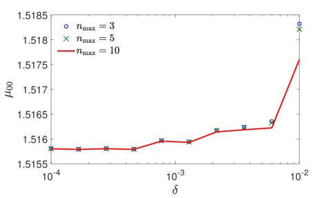
Figure 1: The smallest eigenvalue $\mu_{00}$ of the Dirichlet-to-Neumann operator ${\mathcal{M}}$ for the exterior of the prolate spheroid with semi-axes $a=0.5$ and $b=1$, as a function of the integration step $\delta$ used for approximating the integral (14). Three curves correspond to three truncation orders $n_{\rm max}$ shown on the legend.

The above numerical implementation involves two approximations: the truncation of the matrix ${\bf M}$ (or matrices ${\bf M}_{m}$) and the numerical integration in Eq. (14). We briefly discuss how the accuracy of eigenvalues depends on the truncation order $n_{\rm max}$ and the integration step $\delta$. Since the associated Legendre polynomials $P_{n}^{m}(x)$ oscillate faster as $n$ increases, the integration step has a stronger impact onto larger eigenvalues (i.e., their accuracy is lower). Similarly, the truncation also affects stronger the larger eigenvalues. In other words, an accurate approximation of the eigenvalues $\mu_{mn}$ with large $m$ and $n$ requires taking larger $n_{\rm max}$ and smaller $\delta$. In turn, the eigenvalues with small $m$ and $n$ can be computed very accurately with moderate values of $n_{\rm max}$ and $\delta$. Figure 1 illustrates the dependence of the smallest eigenvalue $\mu_{00}$ on $\delta$ for three truncation orders $n_{\rm max}=3,5,10$. The numerical value of $\mu_{00}$ does not almost change when $\delta\lesssim 5\cdot 10^{-4}$; moreover, it does not almost depend on the considered values of $n_{\rm max}$ in this range. Even in the worst considered case $n_{\rm max}=3$ and $\delta=0.01$, the relative error of this computation is below $0.2\%$. The accuracy may also depend on the aspect ratio $a/b$. In the following, we fix $\delta=10^{-4}$ and $n_{\rm max}=10$. As we focus on first eigenvalues and eigenfunctions, this setting provides very accurate results.

Examples of eigenfunctions

Figure 2 illustrates ten eigenfunctions $v_{mn}$ of the Dirichlet-to-Neumann operator ${\mathcal{M}}$ for the exterior of the prolate spheroid with semi-axes $a=0.5$ and $b=1$. The ground eigenfunction $v_{00}$ is not constant (see below), even though its minor changes are difficult to see due to the chosen colorbar, for which color changes in the same range of values from $-1$ to $1$ for all shown eigenfunctions. The geometric structure of the remaining shown eigenfunctions resembles that of the spherical harmonics $Y_{mn}(\theta,\phi)$. Note that the eigenfunctions $v_{mn}$ and $v_{(-m)n}$ correspond to the same eigenvalue $\mu_{mn}$ and differ only by the factor $e^{\pm im\phi}$; for this reason, the eigenfunctions $v_{(-m)n}$ are not shown.

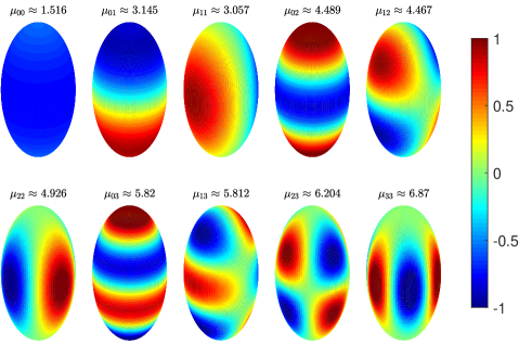
Figure 2: Several eigenfunctions $v_{mn}$ of the Dirichlet-to-Neumann operator ${\mathcal{M}}$ for the exterior of the prolate spheroid with semi-axes $a=0.5$ and $b=1$. The associated eigenvalues are shown on the top. The eigenfunctions with even $m+n$ are symmetric with respect to the horizontal plane $z=0$, whereas the eigenfunctions with odd $m+n$ are antisymmetric, in agreement with Eq. (28). The truncation order is $n_{\rm max}=10$, the integration step is $\delta=10^{-4}$.

Figure 3 shows the behavior of $v_{mn}(\theta,\phi)$ as a function of $\theta$ for $\phi=0$ (i.e., its projection onto the $xz$ plane) for prolate spheroidal surfaces of variables minor semi-axis $a$ (with fixed $b$). As $a\to b$, the surface becomes spherical, and the eigenfunctions $v_{mn}$ coincide with normalized spherical harmonics $Y_{mn}$. In turn, as $a$ decreases, the eigenfunctions $v_{mn}$ deviate further and further from the spherical harmonics. Note that $v_{00}$ and $v_{01}$ are axisymmetric (independent of $\phi$), whereas $v_{11}$ depends on $\phi$, as expected. Table 1 summarizes the first eigenvalues $\mu_{mn}$ for various prolate spheroids.

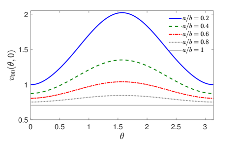
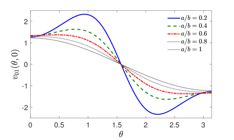
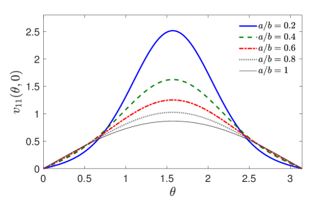
Figure 3: The $xz$ projection of the eigenfunctions $v_{mn}(\theta,\phi)$ of the Dirichlet-to-Neumann operator ${\mathcal{M}}$ for the exterior of the prolate spheroid with semi-axis $a$ and $b=1$, with $mn=00$ (top) $mn=01$ (middle), and $mn=11$ (bottom). Thin line shows the normalized spherical harmonics $Y_{mn}(\theta,0)$ that corresponds to $a/b=1$. The truncation order is $n_{\rm max}=10$.

$a/b$	$\mu_{00}$	$\mu_{01}$	$\mu_{02}$	$\mu_{11}$	$\mu_{12}$	$\mu_{22}$
0.1	3.960	6.787	8.740	11.041	12.764	20.748
0.2	2.558	4.820	6.523	6.035	7.649	10.797
0.3	2.019	4.011	5.577	4.379	5.924	7.513
0.4	1.717	3.514	4.964	3.554	5.034	5.889
0.5	1.516	3.145	4.489	3.057	4.467	4.926
0.6	1.367	2.845	4.093	2.721	4.054	4.288
0.7	1.250	2.588	3.755	2.475	3.726	3.832
0.8	1.153	2.366	3.465	2.285	3.451	3.490
0.9	1.071	2.171	3.216	2.130	3.212	3.220
1.0	1	2	3	2	3	3

Table 1: Several eigenvalues $\mu_{mn}$ of the Dirichlet-to-Neumann operator ${\mathcal{M}}$ for the exterior of the prolate spheroid with semi-axes $a$ and $b=1$. The matrices ${\bf M}_{m}$ are truncated to the size $(n_{\rm max}+1-m)\times(n_{\rm max}+1-m)$, with $n_{\rm max}=10$, while the integration step is $\delta=10^{-4}$. Further increase of $n_{\rm max}$ or decrease of $\delta$ did not change the shown eigenvalues.

Asymptotic behavior for elongated spheroids

In the limit $a\to 0$, prolate spheroids get thinner and thinner, approaching a needle of length $2b$. In this limit, one has $\alpha_{0}\to 0$, and the coefficients $c_{mn}$ diverge in the leading order as

$$c_{mn}\approx\begin{cases}\frac{1}{a\ln(b/a)}\quad(m=0),\cr\frac{|m|}{a}\hskip 28.45274pt(m\neq 0).\end{cases}$$ (26)

In turn, the coefficients $F_{mn,mn^{\prime}}(1)$ are finite. As a consequence, the eigenvalues $\mu_{mn}$ of the matrix ${\bf M}_{m}$ diverge as $a\to 0$ as

$$\mu_{mn}\approx\begin{cases}\frac{q_{n}}{a\,\ln(b/a)}\bigl{(}1+O(1/\ln(b/a))\bigr{)}\quad(m=0),\cr\frac{|m|}{a}\hskip 113.81102pt(m\neq 0),\end{cases}$$ (27)

with some prefactors $q_{n}$. Figure 4 illustrates the behavior of the first eigenvalues $\mu_{mn}$ as functions of the minor semi-axis $a$ (with fixed $b=1$). At $a=1$, one retrieves the eigenvalues $(n+1)/b$ for the exterior of a sphere of radius $b$. In turn, the eigenvalues $\mu_{mn}$ diverge as $a\to 0$ according to Eq. (27). Note that the asymptotic behavior of $\mu_{00}$ is quite accurate with $q_{0}\approx 1$. In turn, logarithmic corrections to the leading order are more significant for $n>0$.

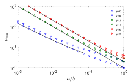
Figure 4: Several eigenvalues $\mu_{mn}$ of the Dirichlet-to-Neumann operator ${\mathcal{M}}$ for the exterior of the prolate spheroid as functions of its minor semi-axis $a$, with $b=1$. At $a=b$, one retrieves the eigenvalues $(n+1)/b$ for the exterior of a sphere of radius $b$. Thin lines from bottom to top present $1/(a\ln(b/a))$, $1/a$ and $2/a$ that capture the asymptotic behavior of $\mu_{mn}$ with $m=0,1,2$, respectively. The eigenvalues are obtained by diagonalizing ${\bf M}_{m}$ truncated to the size $(n_{\rm max}+1-m)\times(n_{\rm max}+1-m)$, with $n_{\rm max}=10$.

Reflection symmetry

Since the domain $\Omega$ is symmetric under reflection with respect to the horizontal plane $z=0$, the Steklov eigenfunctions inherit this symmetry. In fact, if $V(x,y,z)$ is a Steklov eigenfunction, corresponding to an eigenvalue $\mu$, then $V(x,y,-z)$ is also an eigenfunction corresponding to the same $\mu$. Moreover, their linear combinations $V_{\pm}(x,y,z)=V(x,y,z)\pm V(x,y,-z)$ are also eigenfunctions, if they are not zero. There are thus three options: (i) $V(x,y,z)$ is symmetric: $V(x,y,z)=V(x,y,-z)$; (ii) $V(x,y,z)$ is antisymmetric: $V(x,y,z)=-V(x,y,-z)$; or (iii) $V(x,y,z)$ is neither symmetric, nor antisymmetric, in which case $V_{+}(x,y,z)$ and $V_{-}(x,y,z)$ are symmetric and antisymmetric, respectively.

The structure of the matrices ${\bf M}_{m}$ implies that the Steklov eigenfunctions $V_{mn}(\alpha,\theta,\phi)$, determined by Eq. (22b), are symmetric (resp., antisymmetric) under reflection with respect to the horizontal plane $z=0$ when $m+n$ is even (resp., odd). Indeed, the relation (23) causes that the matrix elements ${\bf M}_{mn,mn^{\prime}}$ are zero when $n+n^{\prime}$ is odd. As a consequence, the elements $[{\bf V}_{mn}]_{mn^{\prime}}$ of its eigenvector ${\bf V}_{mn}$ are zero when $n+n^{\prime}$ is odd, so that

$$v_{mn}(\pi-\theta,\phi)=\sum\limits_{n^{\prime}=0}^{\infty}[{\bf V}_{mn}]_{mn^{\prime}}(-1)^{m+n^{\prime}}Y_{mn^{\prime}}(\theta,\phi),$$

where we used $Y_{mn^{\prime}}(\pi-\theta,\phi)=(-1)^{m+n^{\prime}}Y_{mn^{\prime}}(\theta,\phi)$ according to Eq. (23). As the terms with odd $n+n^{\prime}$ vanish, one concludes that

$$v_{mn}(\alpha,\pi-\theta,\phi)=(-1)^{m+n}v_{mn}(\theta,\phi).$$ (28)

This reflection symmetry is clearly illustrated in Fig. 2. The same symmetry is preserved for the Steklov eigenfunctions:

$$V_{mn}(\alpha,\pi-\theta,\phi)=(-1)^{m+n}V_{mn}(\alpha,\theta,\phi).$$ (29)

Half-spheroid in the half-space

The above symmetries provide a complementary insight onto the Steklov problem in the upper half-space. Let

$$\Omega_{+} =\biggl{\{}(x,y,z)\in{\mathbb{R}}^{3}~{}:~{}\frac{x^{2}}{a^{2}}+\frac{y^{2}}{a^{2}}+\frac{z^{2}}{b^{2}}>1,~{}z>0\biggr{\}}$$

$$=\bigl{\{}(\alpha,\theta,\phi)~{}:~{}\alpha>\alpha_{0},~{}0\leq\theta<\pi/2,~{}0\leq\phi<2\pi\bigr{\}}$$

be the exterior of a prolate spheroid in the upper half-space (the second line highlights that the upper half-space corresponds to $0\leq\theta<\pi/2$ in the prolate spheroidal coordinates). The boundary of this domain is the union of the upper half-spheroidal surface,

$$\partial\Omega_{+}=\bigl{\{}(\alpha,\theta,\phi)~{}:~{}\alpha=\alpha_{0},~{}0\leq\theta<\pi/2,~{}0\leq\phi<2\pi\bigr{\}},$$

and the remaining horizontal plane at $z=0$ with a circular hole of radius $a$:

$$\partial\Omega_{0}=\bigl{\{}(\alpha,\theta,\phi)~{}:~{}\alpha>\alpha_{0},~{}\theta=\pi/2,~{}0\leq\phi<2\pi\bigr{\}}.$$

According to Eq. (29), antisymmetric Steklov eigenfunctions $V_{mn}$ (with odd $m+n$) vanish at $\theta=\pi/2$ that corresponds to the Dirichlet boundary condition on $\partial\Omega_{0}$. As a consequence, they solve the mixed Steklov-Dirichlet exterior problem:

$$\Delta V_{mn} =0\quad\textrm{in}~{}\Omega_{+},$$ (30a)

$$\partial_{n}V_{mn} =\mu_{mn}V_{mn}\quad\textrm{on}~{}\partial\Omega_{+},$$ (30b)

$$V_{mn} =0\quad\textrm{on}~{}\partial\Omega_{0}$$ (30c)

(here the notation $\partial_{n}$ for the normal derivative should not be confused with the index $n$). Equivalently, one can speak of eigenvalues $\mu_{mn}$ and eigenfunctions $v_{mn}$ of the Dirichlet-to-Neumann operator ${\mathcal{M}}^{D}$ that maps a given function $f$ on the half-spheroidal boundary $\partial\Omega_{+}$ onto another function $g={\mathcal{M}}^{D}f=(\partial_{n}u)_{|\partial\Omega_{+}}$, where $u$ satisfies

$$\Delta u=0\quad\textrm{in}~{}\Omega_{+},\qquad u|_{\partial\Omega_{+}}=f,\qquad u|_{\partial\Omega_{0}}=0.$$ (31)

For instance, $v_{01}$, $v_{03}$, $v_{12}$ and $v_{23}$ shown in Fig. 2 are examples of eigenfunctions of ${\mathcal{M}}^{D}$.

In turn, the symmetric Steklov eigenfunctions $V_{mn}$ (with even $m+n$) satisfy

$$\left.\bigl{(}\partial_{n}V_{mn}\bigr{)}\right|_{\partial\Omega_{0}}=\left.\biggl{(}\frac{1}{h_{\theta}}\,\partial_{\theta}V_{mn}\biggr{)}\right|_{\theta=\pi/2}=0$$

that corresponds to the Neumann boundary condition on $\partial\Omega_{0}$. In other words, they solve the mixed Steklov-Neumann exterior problem:

$$\Delta V_{mn} =0\quad\textrm{in}~{}\Omega_{+},$$ (32a)

$$\partial_{n}V_{mn} =\mu_{mn}V_{mn}\quad\textrm{on}~{}\partial\Omega_{+},$$ (32b)

$$\partial_{n}V_{mn} =0\quad\textrm{on}~{}\partial\Omega_{0}.$$ (32c)

Equivalently, one can speak of eigenvalues $\mu_{mn}$ and eigenfunctions $v_{mn}$ of the Dirichlet-to-Neumann operator ${\mathcal{M}}^{N}$ that maps a given function $f$ on the half-spheroidal boundary $\partial\Omega_{+}$ onto another function $g={\mathcal{M}}^{N}f=(\partial_{n}u)_{|\partial\Omega_{+}}$, where $u$ satisfies

$$\Delta u=0\quad\textrm{in}~{}\Omega_{+},\qquad u|_{\partial\Omega_{+}}=f,\qquad(\partial_{n}u)|_{\partial\Omega_{0}}=0.$$ (33)

For instance, $v_{00}$, $v_{02}$, $v_{11}$, $v_{22}$, $v_{13}$ and $v_{33}$ shown in Fig. 2 are examples of eigenfunctions of ${\mathcal{M}}^{N}$.

III Oblate spheroids

For the exterior of an oblate spheroid with semi-axes $a\leq b$,

$$\Omega=\biggl{\{}(x,y,z)\in{\mathbb{R}}^{3}~{}:~{}\frac{x^{2}}{b^{2}}+\frac{y^{2}}{b^{2}}+\frac{z^{2}}{a^{2}}>1\biggr{\}},$$ (34)

the computation is very similar so that we only sketch the main steps and formulas. In the oblate spheroidal coordinates $(\alpha,\theta,\phi)$,

$$\left(\begin{array}[]{c}x\\ y\\ z\\ \end{array}\right)=a_{E}\left(\begin{array}[]{c}\cosh\alpha\cos\theta\cos\phi\\ \cosh\alpha\cos\theta\sin\phi\\ \sinh\alpha\sin\theta\\ \end{array}\right)\quad\left\{\begin{array}[]{l}0\leq\alpha<\infty\\ -\tfrac{\pi}{2}\leq\theta\leq\tfrac{\pi}{2}\\ 0\leq\phi<2\pi\\ \end{array}\right\},$$

with $a_{E}=\sqrt{b^{2}-a^{2}}$, the scale factors determining the surface and volume elements, are [43]

$$h_{\alpha} =h_{\theta}=a_{E}\sqrt{\sinh^{2}\alpha+\sin^{2}\theta},$$

$$h_{\phi} =a_{E}\cosh\alpha\cos\theta.$$

In these coordinates, the domain $\Omega$ is still characterized by $\alpha>\alpha_{0}=\tanh^{-1}(a/b)$. A general solution of the Laplace equation reads

$$u(\alpha,\theta,\phi)=\sum\limits_{n=0}^{\infty}\sum\limits_{m=-n}^{n}A_{mn}Q_{n}^{m}(i\sinh\alpha)\bar{Y}_{mn}(\theta,\phi),$$ (35)

where $\bar{Y}_{mn}(\theta,\phi)=a_{mn}P_{n}^{m}(\sin\theta)e^{im\phi}$, and the action of the Dirichlet-to-Neumann operator is

$${\mathcal{M}}u|_{\partial\Omega}=\left.\frac{\partial u}{\partial n}\right|_{\partial\Omega}=-\left.\frac{1}{h_{\alpha}}\partial_{\alpha}u\right|_{\alpha=\alpha_{0}}$$ (36)

$$=\sum\limits_{n=0}^{\infty}\sum\limits_{m=-n}^{n}A_{mn}\bar{Y}_{mn}(\theta,\phi)\frac{\cosh\alpha_{0}\,Q^{{}^{\prime}m}_{n}(i\sinh\alpha_{0})}{ia_{E}\sqrt{\cosh^{2}\alpha_{0}-\cos^{2}\theta}}\,.$$

Multiplying this relation by $\bar{Y}_{m^{\prime}n^{\prime}}^{*}(\theta,\phi)\cos\theta$ and integrating over $\theta$ and $\phi$, one gets a matrix representation of the operator ${\mathcal{M}}$ on the orthonormal basis of $\bar{Y}_{mn}$:

$${\bf M}_{mn,m^{\prime}n^{\prime}}=\bar{F}_{mn,m^{\prime}n^{\prime}}(\sinh\alpha_{0})\,c_{m^{\prime}n^{\prime}},$$ (37)

where

$$c_{mn}=\frac{\cosh\alpha_{0}\,Q^{{}^{\prime}m}_{n}(i\sinh\alpha_{0})}{ia_{E}Q_{n}^{m}(i\sinh\alpha_{0})}$$ (38)

and

$$\bar{F}_{mn,m^{\prime}n^{\prime}}(z) =2\pi\delta_{m,m^{\prime}}a_{mn}a_{m^{\prime}n^{\prime}}\int\limits_{-1}^{1}dx\frac{P_{n}^{m}(x)P_{n^{\prime}}^{m}(x)}{\sqrt{z^{2}+x^{2}}}$$ (39)

$$=iF_{mn,m^{\prime}n^{\prime}}(iz).$$

Since the structure of the matrix ${\bf M}$ is the same as for prolate spheroids, many properties of eigenfunctions of the Dirichlet-to-Neumann operator remain unchanged; in particular, they can be classified according to their dependence on $\phi$ via $e^{im\phi}$; we use the double index $mn$ in the following. Using again the decomposition (20), one can diagonalize separately the submatrices ${\bf M}_{m}$ to access the eigenvalues $\mu_{mn}$ and to construct the eigenfunctions

$$v_{mn}(\theta,\phi)=\sum\limits_{n^{\prime}=0}^{\infty}[{\bf V}_{mn}]_{mn^{\prime}}\bar{Y}_{mn^{\prime}}(\theta,\phi)$$ (40)

and the Steklov eigenfunctions

$$V_{mn}(\alpha,\theta,\phi)=\sum\limits_{n^{\prime}=0}^{\infty}\frac{Q_{n^{\prime}}^{m}(i\sinh\alpha)}{Q_{n^{\prime}}^{m}(i\sinh\alpha_{0})}[{\bf V}_{mn}]_{mn^{\prime}}\bar{Y}_{mn^{\prime}}(\theta,\phi).$$ (41)

As previously, the Steklov eigenfunctions $V_{mn}$ are symmetric for even $m+n$ and antisymmetric for odd $m+n$ under reflection with respect to the horizontal plane $z=0$. In particular, these eigenfunctions solve the mixed Steklov-Neumann and Steklov-Dirichlet exterior problems for the exterior of an oblate spheroid in the upper half-space.

Figure 5 illustrates several eigenfunctions $v_{mn}$ of the Dirichlet-to-Neumann operator ${\mathcal{M}}$ for the exterior of the oblate spheroid with semi-axes $a=0.5$ and $b=1$. Expectedly, these eigenfunctions resemble spherical harmonics $\bar{Y}_{mn}$ but exhibit some differences. In particular, the ground eigenfunction $v_{00}$ is not constant, though its variations are small.

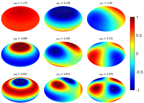
Figure 5: Several eigenfunctions $v_{mn}$ of the Dirichlet-to-Neumann operator ${\mathcal{M}}$ for the exterior of the oblate spheroid with semi-axes $a=0.5$ and $b=1$. The associated eigenvalues are shown on the top. The eigenfunctions with even $m+n$ are symmetric (with respect to the horizontal plane $z=0$), whereas the eigenfunctions with odd $m+n$ are antisymmetric, in agreement with Eq. (28). The truncation order is $n_{\rm max}=10$, the integration step is $\delta=10^{-4}$.

Figure 6 illustrates the behavior of three eigenvalues $\mu_{0n}$ as functions of the minor semi-axis $a$ (with fixed $b=1$). At $a=1$, one retrieves the eigenvalues $(n+1)/b$ for the exterior of a sphere of radius $b$. As $a$ decreases, oblate spheroids become thinner and thinner, approaching a disk of radius $b$. In contrast to the case of prolate spheroids, the eigenvalues are finite in this limit. Curiously, each eigenvalue does not change monotonously with $a$. However, their variations between the disk ($a=0$) and the sphere ($a=b$) are insignificant. Table 2 summarizes several eigenvalues $\mu_{mn}$ for oblate spheroids with the minor semi-axis $a$ ranging from $0$ to $1$ (with $b=1$).

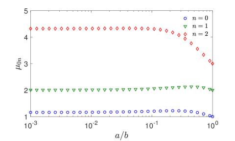
Figure 6: Three eigenvalues $\mu_{0n}$ of the Dirichlet-to-Neumann operator for the exterior of an oblate spheroid as functions of its minor semi-axis $a$, with $b=1$. At $a=b$, one retrieves the eigenvalues $(n+1)/b$ for the exterior of a sphere of radius $b$. As $a\to 0$, one gets the eigenvalues for the exterior of a disk of radius $b$. The axisymmetric matrix ${\bf M}_{0}$ from Eq. (120) was truncated to the size $(n_{\rm max}+1)\times(n_{\rm max}+1)$, with $n_{\rm max}=20$.

$a/b$	$\mu_{00}$	$\mu_{01}$	$\mu_{02}$	$\mu_{11}$	$\mu_{12}$	$\mu_{22}$
0.0	1.158	2.006	4.317	2.755	3.453	4.121
0.1	1.204	2.057	4.317	2.811	3.512	4.197
0.2	1.221	2.094	4.209	2.796	3.539	4.166
0.3	1.217	2.118	4.042	2.732	3.536	4.058
0.4	1.200	2.129	3.852	2.634	3.506	3.900
0.5	1.173	2.129	3.667	2.520	3.453	3.721
0.6	1.141	2.118	3.499	2.401	3.381	3.543
0.7	1.108	2.099	3.351	2.286	3.295	3.379
0.8	1.070	2.072	3.221	2.180	3.200	3.234
0.9	1.034	2.038	3.106	2.085	3.101	3.108
1.0	1	2	3	2	3	3

Table 2: Several eigenvalues $\mu_{mn}$ of the Dirichlet-to-Neumann operator ${\mathcal{M}}$ for the exterior of the oblate spheroid with semi-axes $a$ and $b=1$. The matrices ${\bf M}_{m}$ are truncated to the size $(n_{\rm max}+1-m)\times(n_{\rm max}+1-m)$, with the truncation order $n_{\rm max}=10$ and the integration step $\delta=10^{-4}$. Further increase of $n_{\rm max}$ or decrease of $\delta$ do not change the shown eigenvalues. For the case $a=0$ (a disk), we used the recurrence formulas from Appendix B.2 to construct the matrices ${\bf M}_{m}$ without numerical integration.

Limit of a disk

Let us focus on the limit of the disk when $a=0$ and thus $\alpha_{0}=0$. Its radial coordinate is $r=\sqrt{x^{2}+y^{2}}=b|\cos\theta|$, with $0<\theta<\pi/2$ corresponding to the upper side of the disk, and $-\pi/2<\theta<0$ corresponding to its lower side. Formally, one can set $r=b\cos\theta$ and associate positive $r$ with the upper side of the disk and negative $r$ with its lower side.

As $\alpha_{0}\to 0$, the functions $\bar{F}_{mn,m^{\prime}n^{\prime}}(z)$ from Eq. (39) logarithmically diverge in the limit $z=\sinh\alpha_{0}\to 0$. For any $\alpha_{0}>0$, one can still use the truncated matrix ${\bf M}$ (or ${\bf M}_{m}$) to approximate the eigenvalues and eigenfunctions but larger and larger truncation orders are needed as $\alpha_{0}$ decreases. For this reason, it may be convenient to use an alternative matrix representation, which corresponds to the operator ${\mathcal{M}}^{-1}$ and remains valid even in the limit $\alpha_{0}=0$. This representation is described in Appendix B.2. Importantly, we managed to derive recurrence relations for the elements of this matrix representation that avoids numerical integration. As a consequence, the spectral results for the disk can be obtained much faster and with higher accuracy.

Figure 7 illustrates several eigenfunctions $v_{mn}$ of the Dirichlet-to-Neumann operator for the exterior of the disk of radius $b=1$. One can see that the ground eigenfunction $v_{00}$ shows more significant variations as compared to that shown in Fig. 5. We stress that the eigenfunctions are also present on the bottom side of the disk, which is not visible. Their structure on this hidden side can be easily reconstructed from their symmetry with respect to the horizontal plane: $v_{mn}$ is symmetric (resp., antisymmetric) for even (resp., odd) $m+n$. For instance, the eigenfunction $v_{01}$, which is positive on the upper side of the disk, takes negative values on the bottom side.

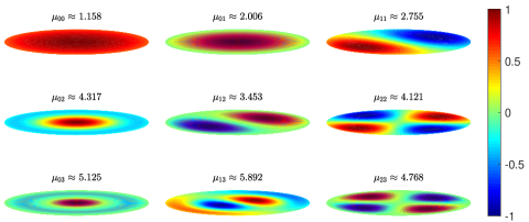
Figure 7: Several eigenfunctions $v_{mn}$ of the Dirichlet-to-Neumann operator ${\mathcal{M}}$ for the exterior of the disk of radius $b=1$. The associated eigenvalues are shown on the top. Normalization by the maximum of $|v_{mn}|$ was employed for a better visualization. The symmetric (resp., antisymmetric) shape of the eigenfunction $v_{mn}$ for even (resp., odd) $m+n$ allows one to reconstruct its structure on the bottom side of the disk, which is not visible. The truncation order is $n_{\rm max}=10$, and we used the recurrence formulas from Appendix B.2 to construct the matrices ${\bf M}_{m}$ without numerical integration.

Axisymmetric setting

Let us briefly discuss the action of the Dirichlet-to-Neumann operator onto rotationally invariant functions that do not depend on the angle $\phi$. If a function $f(\theta)$ is decomposed on the normalized Legendre polynomials $\psi_{n}(\theta)=\sqrt{n+1/2}\,P_{n}(\sin\theta)$,

$$f(\theta)=\sum\limits_{n=0}^{\infty}f_{n}\psi_{n}(\theta),$$ (42)

the action of ${\mathcal{M}}$ reads

$${\mathcal{M}}f=\sum\limits_{n=0}^{\infty}f_{n}\psi_{n}(\theta)\frac{c_{0n}}{b\sqrt{1-\cos^{2}\theta}}\,.$$ (43)

Setting $b=1$ for simplicity and using $r=\cos\theta$, we get, for instance,

$${\mathcal{M}}1 =\frac{c_{00}}{\sqrt{1-r^{2}}}\,,$$ (44a)

$${\mathcal{M}}\sqrt{1-r^{2}} =c_{01},$$ (44b)

where

$$c_{0n}=\frac{-iQ^{\prime}_{n}(0)}{Q_{n}(0)}=2\biggl{(}\frac{\Gamma(n/2+1)}{\Gamma(n/2+1/2)}\biggr{)}^{2}$$ (45)

(see Appendix B.4 for details). For instance, $c_{00}=2/\pi$, $c_{01}=\pi/2$, $c_{02}=8/\pi$, $c_{03}=9\pi/8$, etc. The first relation (44a) reproduces the classical Weber’s solution for the electric current density onto a conducting disk [44], see below.

Alternatively, setting $x=\sin\theta$, one has

$${\mathcal{M}}P_{n}(x)=c_{0n}\frac{P_{n}(x)}{|x|}\qquad(-1<x<1).$$ (46)

One sees that ${\mathcal{M}}P_{n}(x)$ keeps the parity of $P_{n}(x)$, i.e., it is symmetric for even $n$ and antisymmetric for odd $n$. For instance, one has

$${\mathcal{M}}1 =\frac{2}{\pi}\,\frac{1}{|x|}\,,$$

$${\mathcal{M}}x =\frac{\pi}{2}\,\frac{x}{|x|}\,,$$

$${\mathcal{M}}x^{2} =\frac{2}{\pi}\,\frac{4x^{2}-1}{|x|}\,.$$

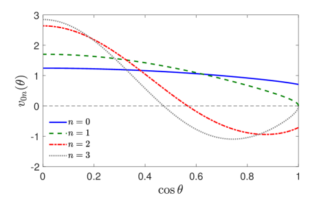
Figure 8: Four eigenfunctions $v_{0n}(\theta)$ of the Dirichlet-to-Neumann operator for the exterior of a disk of radius $b=1$, as a function of $r=b\cos\theta$. The associated eigenvalues are $1.158$, $2.006$, $4.317$, and $5.125$. The axisymmetric matrix ${\bf M}_{0}$ is truncated to $(n_{\rm max}+1)\times(n_{\rm max}+1)$, with $n_{\rm max}=20$.

Disk in the half-space

The general representation (35) allows one to solve boundary value problems (31, 33) in the upper half-space, by imposing Dirichlet or Neumann boundary condition on $\partial\Omega_{0}$. In the case of a disk of radius $b$, the first problem actually concerns the Dirichlet boundary condition on the horizontal plane, for a class of functions $f(r)$ that are strictly zero for $r\geq b$. Its solution can be written in the integral form:

$$u(x_{0},y_{0},z_{0}) =\int\limits_{x^{2}+y^{2}<b^{2}}dx\,dy\,f(x,y)$$

$$\times\frac{z_{0}}{2\pi(z_{0}^{2}+(x-x_{0})^{2}+(y-y_{0})^{2})^{3/2}}\,,$$ (47)

where the factor in front of $f$ is the harmonic measure density [45]. Alternatively, one can use the representation (35) of a harmonic function in oblate spheroidal coordinates, in which the coefficients $A_{mn}$ are obtained by setting $\alpha=0$, multiplying by $\bar{Y}_{mn}^{*}\cos\theta$ and integrating over $\theta$ and $\phi$:

$$A_{mn}=\frac{1}{Q_{n}^{m}(0)}\int\limits_{-\pi/2}^{\pi/2}d\theta\int\limits_{0}^{2\pi}d\phi\,f(\theta,\phi)\,\bar{Y}_{mn}^{*}(\theta,\phi)\cos\theta.$$ (48)

For instance, if $f(\theta,\phi)=\textrm{sign}(\theta)$, one gets

$$A_{mn} =\frac{2\pi\delta_{m,0}a_{0n}}{Q_{n}^{m}(0)}\int\limits_{-1}^{1}dx\,\textrm{sign}(x)\,P_{n}(x)$$

$$=\frac{2\pi\delta_{m,0}a_{0n}}{Q_{n}^{m}(0)}\,\frac{P_{n-1}(0)-P_{n+1}(0)}{n+1/2}$$ (49)

for odd $n$, where $P_{2n}(0)=\frac{(-1)^{n}(2n)!}{2^{2n}(n!)^{2}}$. As a consequence, one has

$$u=\sum\limits_{n=0}^{\infty}\frac{Q_{2n+1}(i\sinh\alpha)}{Q_{2n+1}(0)}P_{2n+1}(\sin\theta)\bigl{(}P_{2n}(0)-P_{2n+2}(0)\bigr{)}\,.$$ (50)

This is also the solution of the Laplace equation in the upper half space with the boundary condition $u|_{z=0}=\Theta(b-r)$, where $\Theta(z)$ is the Heaviside step function: $\Theta(z)=1$ for $z>0$ and $0$ otherwise. This is the splitting probability for the disk of radius $b$, i.e., the probability that a particle started from a point $(\alpha,\theta,\phi)$ hits the disk before hitting its complement (the horizontal plane without this disk) [45, 46, 47].

In the same vein, the representation (35) with even $m+n$ allows one to solve the mixed Dirichlet-Neumann boundary value problem (33) in the upper half-space, with coefficients $A_{mn}$ given by Eq. (48). For instance, if $f=1$, one gets

$$A_{mn}=\frac{2\sqrt{\pi}\delta_{m,0}\delta_{n,0}}{Q_{n}(0)}\,,$$ (51)

so that

$$u=\frac{Q_{0}(i\sinh\alpha)}{Q_{0}(0)}\,,$$ (52)

where $\alpha=\cosh^{-1}((r_{+}+r_{-})/(2b))$, with $r_{\pm}=\sqrt{(r\pm b)^{2}+z^{2}}$. This expression can be written more explicitly as

$$u(r,z)=\frac{1}{\pi}\cos^{-1}\biggl{(}1-\frac{8b^{2}}{(r_{+}+r_{-})^{2}}\biggr{)}.$$ (53)

It is worth noting that the mixed Dirichlet-Neumann boundary value problem for rotationally invariant functions $f(r)$,

$$\Delta u=0\quad(z>0),\quad\left\{\begin{array}[]{ll}u(r,0)=f(r)&(0\leq r<b),\\ (\partial_{z}u(r,z))|_{z=0}=0&(r>b),\\ \end{array}\right.$$ (54)

was solved by Beltrami via integral representations (see [44], page 66):

$$u(r,z)=\int\limits_{0}^{\infty}d\xi\,A(\xi)\,e^{-z\xi}\,J_{0}(\xi r),$$ (55)

where

$$A(\xi)=\int\limits_{0}^{1}ds\,\cos(\xi s)\frac{d}{ds}\left(\frac{2}{\pi}\int\limits_{0}^{s}dt\,\frac{t\,f(tb)}{\sqrt{s^{2}-t^{2}}}\right).$$ (56)

For instance, setting $f(r)=1$, one retrieves the Weber’s solution for the electric potential around a conducting disk:

$$u(r,z)=\frac{2}{\pi}\int\limits_{0}^{\infty}\frac{d\xi}{\xi}\sin(\xi b)\,e^{-\xi z}\,J_{0}(\xi r),$$ (57)

from which

$$-(\partial_{n}u)|_{\partial\Omega_{+}}=\frac{2}{\pi\sqrt{b^{2}-r^{2}}}\qquad(0\leq r<b).$$ (58)

One sees that the above expressions (52) and (53) are more explicit than the equivalent integral representation (57). In probabilistic terms, $1-u(r,z)$ is the escape (or survival) probability for a particle started from a point $(r,z)$, which can be destroyed upon its first arrival onto the absorbing disk. Alternatively, $C_{0}u(r,z)$ can be understood as the concentration of particles diffusing from infinity (with a concentration $C_{0}$) towards an absorbing disk. In this light, $j=-DC_{0}(\partial_{n}u)|_{\partial\Omega_{+}}$ is the diffusive flux density onto the disk. Dividing this expression by the total flux, one gets the harmonic measure density on the absorbing disk for a particle started from infinity:

$$\omega(r)=\frac{DC_{0}\frac{2}{\pi\sqrt{b^{2}-r^{2}}}}{DC_{0}\frac{2}{\pi}b}=\frac{1}{b\sqrt{b^{2}-r^{2}}}\,.$$ (59)

IV Two applications

As mentioned in Sec. I, the Dirichlet-to-Neumann operator ${\mathcal{M}}$ and its eigenfunctions have found numerous applications in applied mathematics and engineering. Here we briefly discuss two applications in physics. In Sec. IV.1, we start with diffusion-controlled reactions in chemical physics and illustrate the use of ${\mathcal{M}}$ for representing the Robin boundary condition that is often used to describe surface reactions on partially reactive targets. In Sec. IV.2, we highlight their relation to the statistics of encounters between a diffusing particle and the boundary, which is relevant in statistical physics and in the theory of reflected Brownian motion.

IV.1 Partially reactive boundaries

Diffusion-controlled reactions play an important role in physics, chemistry and biology [48, 49, 50, 51, 52, 53, 54, 55, 56, 57, 58]. In the idealized setting introduced by Smoluchowski [59], a reactant diffuses towards its partner or towards a catalytic surface, and reacts upon their first encounter. In many situations, however, the first encounter is not sufficient, as the reactant and/or its partner may need to overcome an activation energy barrier, to be in an appropriate “active” state, to arrive onto a specific catalytic germ, to pass through a channel/pore, etc. [58]. If any of these conditions is failed, the reactant resumes its bulk diffusion until the next encounter, and so on. Starting from Collins and Kimball [60], such partial reactions are described by imposing the Robin boundary condition, in which the diffusive flux of particles towards the catalytic boundary is postulated to be proportional to their concentration on that boundary. In other words, the concentration $C$ of diffusing reactants in the steady-state regime obeys:

$$\Delta C =0\quad\textrm{in}~{}\Omega,$$ (60a)

$$-D\partial_{n}C =\kappa C\quad\textrm{on}~{}\partial\Omega,$$ (60b)

$$\lim\limits_{|\bm{x}|\to\infty}C =C_{0},$$ (60c)

where $D$ is the diffusion coefficient, $\kappa\geq 0$ is a constant reactivity of the boundary, and $C_{0}$ is the initial concentration maintained at infinity. Setting $q=\kappa/D$ and $C=C_{0}(1-u)$, one can express the Robin boundary condition $\partial_{n}u+qu=q$ on $\partial\Omega$ with the help of the Dirichlet-to-Neumann operator:

$$u|_{\partial\Omega} =({\mathcal{M}}+q)^{-1}q$$

$$=\sum\limits_{k=0}^{\infty}\frac{(v_{k},1)_{L^{2}(\partial\Omega)}}{\|v_{k}\|^{2}_{L^{2}(\partial\Omega)}}\,\frac{q}{\mu_{k}+q}\,v_{k},$$ (61)

where we used the completeness of the basis of the eigenfunctions $\{v_{k}\}$.

For prolate spheroids, a general solution (6) of the Laplace equation can be written as

$$u(\alpha,\theta,\phi)=\sum\limits_{m,n}f_{mn}\frac{Q_{n}^{m}(\cosh\alpha)}{Q_{n}^{m}(\cosh\alpha_{0})}Y_{mn}(\theta,\phi),$$ (62)

where the coefficients $f_{mn}$ are found from the restriction of $u$ onto $\partial\Omega$ as:

$$f_{mn} =\int\limits_{0}^{\pi}d\theta\int\limits_{0}^{2\pi}d\phi\,\sin\theta\,Y_{mn}^{*}(\theta,\phi)\,u|_{\partial\Omega}$$

$$=\sum\limits_{k=0}^{\infty}\frac{(v_{k},1)_{L^{2}(\partial\Omega)}}{\|v_{k}\|^{2}_{L^{2}(\partial\Omega)}}\,\frac{q}{\mu_{k}+q}$$

$$\times\int\limits_{0}^{\pi}d\theta\int\limits_{0}^{2\pi}d\phi\,\sin\theta\,Y_{mn}^{*}(\theta,\phi)\,v_{k}(\theta,\phi)$$

$$=\sum\limits_{k=0}^{\infty}\frac{(v_{k},1)_{L^{2}(\partial\Omega)}}{\|v_{k}\|^{2}_{L^{2}(\partial\Omega)}}\,\frac{q}{\mu_{k}+q}[{\bf V}_{k}]_{mn},$$ (63)

where we employed the representation (15). Using Eqs. (106, 110), one can further simplify:

$$f_{mn} =\frac{\sqrt{4\pi}}{a_{E}\sinh\alpha_{0}Q_{0}(\cosh\alpha_{0})}\sum\limits_{k=0}^{\infty}\frac{[{\bf V}_{k}^{*}]_{00}[{\bf V}_{k}]_{mn}}{({\bf V}_{k}^{\dagger}{\bf c}{\bf V}_{k})}\,\frac{q}{\mu_{k}+q}$$

$$=\sqrt{4\pi}\sum\limits_{k=0}^{\infty}\frac{[\tilde{{\bf V}}_{k}^{*}]_{00}[\tilde{{\bf V}}_{k}]_{mn}}{(\tilde{{\bf V}}_{k}^{\dagger}\tilde{{\bf V}}_{k})}\,\frac{q}{\mu_{k}+q}\,,$$ (64)

where $\tilde{{\bf V}}_{k}={\bf c}^{\frac{1}{2}}{\bf V}_{k}$ (we recall that the diagonal matrix ${\bf c}$ is formed by $c_{mn}$). Since $\mu_{k}$ and $\tilde{{\bf V}}_{k}$ are eigenvalues and eigenvectors of the Hermitian matrix $\tilde{{\bf M}}={\bf c}^{\frac{1}{2}}{\bf M}{\bf c}^{-\frac{1}{2}}$, one can also rewrite the above expression in a matrix form:

$$f_{mn}=\sqrt{4\pi}\,q\bigl{[}(\tilde{{\bf M}}+q{\bf I})^{-1}\bigr{]}_{mn,00},$$ (65)

where ${\bf I}$ is the identity matrix. Note that the matrix $\tilde{{\bf M}}$ can be replaced by $\tilde{{\bf M}}_{0}={\bf c}^{\frac{1}{2}}{\bf M}_{0}{\bf c}^{-\frac{1}{2}}$ due to the axial symmetry of the problem. Similar representation were discussed in [40, 17].

Knowing the concentration, one can easily deduce the total diffusive flux onto the boundary:

$$J_{q} =\int\limits_{\partial\Omega}(-D\partial_{n}C)=DC_{0}\int\limits_{\partial\Omega}(\partial_{n}u)|_{\partial\Omega}$$

$$=DC_{0}q\bigl{(}1,{\mathcal{M}}({\mathcal{M}}+q)^{-1}1\bigr{)}_{L^{2}(\partial\Omega)}$$

$$=DC_{0}q\sum\limits_{k=0}^{\infty}\frac{|(1,v_{k})_{L^{2}(\partial\Omega)}|^{2}}{\|v_{k}\|^{2}_{L^{2}(\partial\Omega)}}\,\frac{\mu_{k}}{\mu_{k}+q}$$

$$=\frac{4\pi DC_{0}q}{\sinh\alpha_{0}Q_{0}^{2}(\cosh\alpha_{0})}\sum\limits_{k=0}^{\infty}\frac{[{\bf V}_{k}^{*}]_{00}\,[{\bf V}_{k}]_{00}}{({\bf V}_{k}^{\dagger}{\bf c}{\bf V}_{k})}\,\frac{1}{\mu_{k}+q}$$

$$=\frac{4\pi DC_{0}a_{E}q}{Q_{0}(\cosh\alpha_{0})}\sum\limits_{k=0}^{\infty}\frac{[\tilde{{\bf V}}_{k}^{*}]_{00}\,[\tilde{{\bf V}}_{k}]_{00}}{(\tilde{{\bf V}}_{k}^{\dagger}\tilde{{\bf V}}_{k})}\,\frac{1}{\mu_{k}+q}$$

$$=\frac{4\pi DC_{0}a_{E}q}{Q_{0}(\cosh\alpha_{0})}\bigl{[}(\tilde{{\bf M}}+q{\bf I})^{-1}\bigr{]}_{00,00}.$$ (66)

In the limit $q\to\infty$, one formally retrieves the classical result for a perfectly reactive prolate spheroid (see, e.g., [40]):

$$J_{\infty}=\frac{4\pi DC_{0}a_{E}}{Q_{0}(\cosh\alpha_{0})}\,.$$ (67)

As a consequence, the effect of partial reactivity is represented by $q\bigl{[}(\tilde{{\bf M}}+q{\bf I})^{-1}\bigr{]}_{00,00}$. In the limit of a sphere ($a\to b$), this factor reduces to $q/(q+1/b)$ so that one retrieves the Collins-Kimball diffusive flux [60]

$$J_{q}=4\pi DC_{0}b\,\frac{qb}{1+qb}\qquad(a=b),$$ (68)

where $4\pi DC_{0}b$ is the Smoluchowski diffusive flux $J_{\infty}$ onto a perfectly reactive sphere of radius $b$ [59].

For oblate spheroids, a similar computation involves

$$u(\alpha,\theta,\phi)=\sum\limits_{m,n}f_{mn}\frac{Q_{n}^{m}(i\sinh\alpha)}{Q_{n}^{m}(i\sinh\alpha_{0})}\bar{Y}_{mn}(\theta,\phi),$$ (69)

with the same expression (65) for the coefficients $f_{mn}$. The total diffusive flux reads

$$J_{q}=\underbrace{\frac{4\pi DC_{0}a_{E}}{iQ_{0}(i\sinh\alpha_{0})}}_{=J_{\infty}}~{}q\bigl{[}(\tilde{{\bf M}}+q{\bf I})^{-1}\bigr{]}_{00,00}\,.$$ (70)

In the case of a disk, this quantity was thoroughly studied in [61].

Figure 9 illustrates the behavior of the diffusive flux $J_{q}$, rescaled by $J_{\infty}$, as a function of the reactivity parameter $q$. Expectedly, this ratio changes from $0$ at $q=0$ (no surface reaction) to $1$ at $q\to\infty$ (perfect surface reaction). For prolate spheroids, their anisotropy reduces the diffusive flux monotonously (curves are shifted downwards as $a/b$ decreases). As the spheroid gets thinner, its accessibility to Brownian motion is reduced, and this effect is enhanced by decreasing the reactivity $q$ and thus requiring more and more returns to the target to realize a successful reaction. The situation is more subtle for oblate spheroids. Even in the limit $a=0$, the disk remains accessible to Brownian motion so that the effect of anisotropy onto the diffusive flux is moderate (all shown curves are close to each other). Curiously, the reduction of the diffusive flux by anisotropy is not monotonous for oblate spheroids. For instance, one can notice that the curves for $a/b=0.01$ and $a/b=0.2$ cross each other. In other words, if the ratio $J_{q}/J_{\infty}$ was plotted as a function of $a/b$ (not shown), it would exhibit a minimum at some intermediate aspect ratio that depends on the reactivity parameter $q$. This behavior can be a consequence of the non-monotonous dependence of eigenvalues $\mu_{mn}$ of the Dirichlet-to-Neumann operator on the aspect ratio $a/b$, as illustrated in Fig. 6.

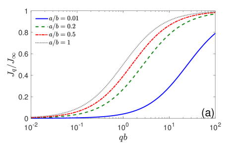
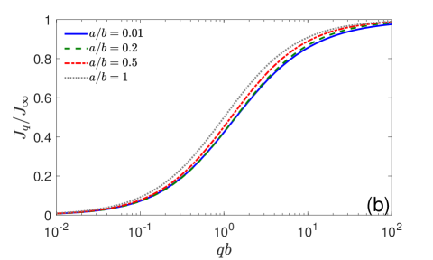
Figure 9: The diffusive flux $J_{q}$ onto a partially reactive spheroidal boundary with semi-axes $a$ and $b$, rescaled by $J_{\infty}$. Panels (a) and (b) present $J_{q}$ for prolate and oblate spheroids, respectively. The matrix $\tilde{{\bf M}}$ in Eqs. (66, 70) was truncated to the size $(n_{\rm max}+1)^{2}\times(n_{\rm max}+1)^{2}$, with $n_{\rm max}=10$.

More generally, the Dirichlet-to-Neumann operator and its matrix representation allow one to investigate the effect of spatially heterogeneous reactivity when $q$ changes on the boundary [17]. In addition, one can use the Steklov eigenfunctions to compute the Green’s function with the Robin boundary condition.

IV.2 Statistics of boundary encounters

The Steklov eigenfunctions also play the central role in the encounter-based approach to diffusion-controlled reactions [18]. In this context, one usually considers a more general setting, in which the Laplace equation (1) is replaced by the modified Helmholtz equation, $(p-D\Delta)u=0$, with $p\geq 0$. The eigenfunctions of the related Steklov problem determine the spectral expansion of the Laplace transform of the encounter propagator $P(\bm{x},\ell,t|\bm{x}_{0})$, i.e., the joint probability density of the position $\bm{X}_{t}$ and the boundary local time $\ell_{t}$ of a particle that starts from a point $\bm{x}_{0}$ and diffuses in a domain $\Omega$ with the reflecting boundary $\partial\Omega$ [18]. Here the boundary local time $\ell_{t}$ can be understood as the (rescaled) number of encounters between the diffusing particle and the boundary, which is crucial for describing various phenomena occuring on the boundary [20, 23, 21, 22]. The encounter propagator allows one to access most common characteristics of diffusion-controlled reactions, including the conventional propagator, the survival probability, the first-passage time probability density, the harmonic measure density, the diffusive flux, etc. For instance, the integral over the boundary $\partial\Omega$ gives the probability density of the first-crossing time $\tau=\inf\{t>0~{}:~{}\ell_{t}>\ell\}$ of a threshold $\ell$ by $\ell_{t}$ [18]:

$$\frac{{\mathbb{P}}_{\bm{x}_{0}}\{\tau\in(t,t+dt)\}}{dt}=U(\ell,t|\bm{x}_{0})=D\int\limits_{\partial\Omega}d\bm{x}\,P(\bm{x},\ell,t|\bm{x}_{0}).$$ (71)

In other words, the random variable $\tau$ is the first time instance when the number of encounters exceeds a given threshold. For a bounded domain, any threshold is crossed with probability $1$ so that the probability density $U(\ell,t|\bm{x}_{0})$ is normalized to $1$. However, when a three-dimensional domain is unbounded, the particle can escape to infinity and never return to the boundary $\partial\Omega$. As a consequence, the integral of $U(\ell,t|\bm{x}_{0})$ over $t$ may be smaller than $1$; in fact, this integral determines the probability of crossing of a given threshold $\ell$:

$${\mathbb{P}}_{\bm{x}_{0}}\{\ell_{\infty}>\ell\}=\int\limits_{0}^{\infty}dt\,U(\ell,t|\bm{x}_{0}).$$ (72)

One can therefore employ the general spectral expansion of the Laplace-transformed encounter propagator, derived in [18], to determine this probability in terms of the Steklov eigenfunctions for the Laplace equation that we studied here:

$${\mathbb{P}}_{\bm{x}_{0}}\{\ell_{\infty}>\ell\}=\sum\limits_{k=0}^{\infty}[V_{k}(\bm{x}_{0})]^{*}e^{-\mu_{k}\ell}\int\limits_{\partial\Omega}d\bm{x}\,v_{k}(\bm{x}).$$ (73)

At $\ell=0$, this is simply the probability of hitting the boundary (before escaping to infinity). At large $\ell$, this probability decays exponentially, and the rate of this decay is given by the smallest eigenvalue $\mu_{0}$. When prolate spheroids get thinner ($a\to 0$), the eigenvalue $\mu_{0}$ diverges according to Eq. (27), so that the crossing probability ${\mathbb{P}}_{\bm{x}_{0}}\{\ell_{\infty}>\ell\}$ decays faster with $\ell$. Indeed, it is hard for Brownian motion to access thin prolate spheroids, and it is therefore unlikely to experience many encounters (i.e., to get large $\ell_{t}$). In turn, the eigenvalue $\mu_{0}$ approaches a constant value in the opposite limit of thin oblate spheroids. This is consistent with the fact that even a disk ($a=0$) remains accessible to Brownian motion in three dimensions. Other properties of the limiting boundary local time $\ell_{\infty}$ can be investigated using our results.

V Conclusions

In this paper, we investigated the spectral properties of the Dirichlet-to-Neumann operator ${\mathcal{M}}$ and the related Steklov problem for anisotropic domains in three dimensions. Using prolate and oblate spheroidal coordinates, we derived a matrix representation of ${\mathcal{M}}$ on the basis of spherical harmonics for both exterior and interior problems. Its diagonalization allowed us to access the eigenvalues $\mu_{mn}$ and eigenfunctions $v_{mn}$ of ${\mathcal{M}}$, as well as the Steklov eigenfunctions $V_{mn}$. These eigenfunctions inherited the symmetries of the considered domains; in particular, $V_{mn}$ depend on the angle $\phi$ via the factor $e^{im\phi}$, and are symmetric (resp., antisymmetric) with respect to the horizontal plane $z=0$ when $m+n$ is even (resp., odd). As a consequence, they are also the eigenfunctions of the mixed Steklov-Neumann (resp., Steklov-Dirichlet) problems in the upper half-space. We also described recurrence relations to speed up the numerical construction of truncated matrices. While the interior spectral problem in a bounded domain could alternatively be solved by other numerical methods [62, 63, 64, 65, 66, 67, 68, 69, 70, 71, 72], exterior spectral problems in unbounded domains are in general more difficult to address by conventional tools.

We discussed the impact of domain anisotropy onto the behavior of eigenvalues and eigenfunctions. In particular, we showed how the eigenvalues of ${\mathcal{M}}$ for the exterior of a prolate spheroid diverge in the limit $a\to 0$ (the exterior of a needle); in turn, in the opposite limit of thin (disk-like) oblate spheroids, the eigenvalues reach finite values. In this limit, we also got complementary insights onto a classical mixed Dirichlet-Neumann problem in the half-space.

Apart from their own fundamental interest in spectral geometry, the Steklov eigenfunctions offer flexible meshless representations for solutions of interior and exterior boundary value problems. In the context of diffusion-controlled reactions, these eigenfunctions allow one to incorporate the effect of partial reactivity, e.g., to compute the steady-state concentration of particles that react on the spheroidal boundary. In particular, we showed how the total diffusive flux (i.e., the overall reaction rate) depends on the anisotropy of the target. Another application from statistical physics concerns the statistics of encounters between a diffusing particle and the spheroidal target. The Steklov eigenfunctions determine the crossing probability ${\mathbb{P}}_{\bm{x}_{0}}\{\ell_{\infty}>\ell\}$, i.e., the probability that the (rescaled) number of encounters, $\ell_{\infty}$, exceeds a given threshold $\ell$, before the particle escapes to infinity. The crossing probability generalizes the hitting probability of the target (the latter corresponding to $\ell=0$). In particular, we showed that the smallest eigenvalue $\mu_{00}$ of the Dirichlet-to-Neumann operator determines the exponential decay of the crossing probability at large thresholds $\ell$.

In summary, this study brings novel insights onto the spectral properties of the Dirichlet-to-Neumann operator for exterior domains, with the special emphasis on anisotropy. Even though the derived eigenvalues and eigenfunctions are not as explicit as in the case of the exterior of a ball, the matrix representation offers an efficient numerical computation and allows for getting asymptotic results. One straightforward extension of this study concerns diffusion across a semi-permeable spheroidal boundary, which is a model of diffusive exchange in anisotropic living cells or tissues [74, 75, 76]. The exchange between interior and exterior compartments is usually described by a transmission boundary condition that can be reformulated in terms of two Dirichlet-to-Neumann operators for the interior and exterior problems. Moreover, an extension of the encounter-based approach to semi-permeable membranes allows one to treat much more sophisticated exchange mechanisms [77, 78, 79, 80]. Another promising direction is related to the Dirichlet-to-Neumann operator for the (modified) Helmholtz equation. As briefly discussed in Sec. IV.2, the related Steklov eigenfunctions determine the encounter propagator and thus most diffusion-reaction characteristics in this system. While one could employ prolate/oblate spheroidal wave functions, their analysis is more sophisticated and less explicit. Alternatively, one can consider other domains, in which the Laplace operator admits separation of variables in appropriate curvilinear coordinates (e.g., a torus). A systematic investigation of the Dirichlet-to-Neumann operator in such relatively simple shapes can help to uncover the intricate relations between the geometry and the spectral properties of this operator.

Appendix A Interior problems

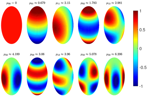
Figure 10: Several eigenfunctions $v_{mn}$ of the Dirichlet-to-Neumann operator ${\mathcal{M}}$ for the interior of the prolate spheroid with semi-axes $a=0.5$ and $b=1$. The associated eigenvalues are shown on the top. The truncation order is $n_{\rm max}=10$, the integration step is $\delta=10^{-4}$.

While the main text is focused on exterior problems, the same approach is valid for the interior spectral problems when the Laplace equation has to solved inside a bounded prolate or oblate spheroid. In fact, the coefficients $F_{mn,m^{\prime}n^{\prime}}(z)$ and $\bar{F}_{mn,m^{\prime}n^{\prime}}(z)$ remain unchanged, and the difference between exterior and interior settings is only manifested in the coefficients $c_{mn}$:

(i) for prolate spheroids, it is sufficient to replace $Q_{n}^{m}(z)$ by $P_{n}^{m}(z)$ in Eq. (11), as well as the sign:

$$c_{mn}=\frac{\sinh\alpha_{0}\,P^{{}^{\prime}m}_{n}(\cosh\alpha_{0})}{a_{E}P_{n}^{m}(\cosh\alpha_{0})}\,.$$ (74)

(ii) for oblate spheroids, it is sufficient to replace $Q_{n}^{m}(z)$ by $P_{n}^{m}(z)$ in Eq. (38), as well as the sign:

$$c_{mn}=\frac{i\cosh\alpha_{0}\,P^{{}^{\prime}m}_{n}(i\sinh\alpha_{0})}{a_{E}P_{n}^{m}(i\sinh\alpha_{0})}\,.$$ (75)

In both cases, as $P^{\prime}_{0}=0$ and thus $c_{00}=0$, one can easily check that the first eigenvalue is zero, $\mu_{00}=0$, as it should be.

Figures 10 and 11 illustrate several eigenfunctions $v_{mn}$ for the interior prolate/oblate spheroid with semi-axes $a=0.5$ and $b=1$. The associated eigenvalues $\mu_{mn}$ are shown on the top of each panel. Expectedly, a constant eigenfunction $v_{00}$ corresponds to $\mu_{00}=0$. Other eigenfunctions also resemble the spherical harmonics.

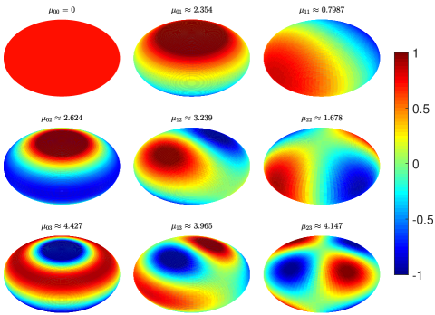
Figure 11: Several eigenfunctions $v_{mn}$ of the Dirichlet-to-Neumann operator ${\mathcal{M}}$ for the interior of the oblate spheroid with semi-axes $a=0.5$ and $b=1$. The associated eigenvalues are shown on the top. The truncation order is $n_{\rm max}=10$, the integration step is $\delta=10^{-4}$.

One can also consider more sophisticated domains confined between two confocal prolate (oblate) spheroids. These domains are characterized as $\alpha_{1}<\alpha<\alpha_{2}$, where $\alpha_{1}=\tanh^{-1}(a/b)$ and $\alpha_{2}=\tanh^{-1}(A/B)$, with $a,b$ and $A,B$ being the semi-axes of the inner and outer boundaries such that $a_{E}=\sqrt{b^{2}-a^{2}}=\sqrt{B^{2}-A^{2}}$ is half of the focal distance for both boundaries. In this case, a general solution of the Laplace equation involves both $P_{n}^{m}(z)$ and $Q_{n}^{m}(z)$ but the structure of the matrix representation is very similar. We just mention two settings, in which either Dirichlet or Neumann boundary condition is imposed on the outer boundary, whereas the inner boundary has the Steklov condition (the opposite setting can be easily obtained).

(i) For prolate spheroids, the matrix ${\bf M}$ is still given by Eq. (13), in which $\alpha_{0}$ is replaced by $\alpha_{1}$, and the coefficients $c_{mn}$ depend on the boundary condition on the outer spheroid:

$$c_{mn}=-\frac{\sinh\alpha_{1}}{a_{E}}\,\frac{P_{n}^{m}(\cosh\alpha_{2})Q_{n}^{{}^{\prime}m}(\cosh\alpha_{1})-Q_{n}^{m}(\cosh\alpha_{2})P_{n}^{{}^{\prime}m}(\cosh\alpha_{1})}{P_{n}^{m}(\cosh\alpha_{2})Q_{n}^{m}(\cosh\alpha_{1})-Q_{n}^{m}(\cosh\alpha_{2})P_{n}^{m}(\cosh\alpha_{1})}\qquad\textrm{(Dirichlet),}$$ (76)

$$c_{mn}=-\frac{\sinh\alpha_{1}}{a_{E}}\,\frac{P_{n}^{{}^{\prime}m}(\cosh\alpha_{2})Q_{n}^{{}^{\prime}m}(\cosh\alpha_{1})-Q_{n}^{{}^{\prime}m}(\cosh\alpha_{2})P_{n}^{{}^{\prime}m}(\cosh\alpha_{1})}{P_{n}^{{}^{\prime}m}(\cosh\alpha_{2})Q_{n}^{m}(\cosh\alpha_{1})-Q_{n}^{{}^{\prime}m}(\cosh\alpha_{2})P_{n}^{m}(\cosh\alpha_{1})}\qquad\textrm{(Neumann).}$$ (77)

(ii) For oblate spheroids, the matrix ${\bf M}$ is still given by Eq. (37), in which $\alpha_{0}$ is replaced by $\alpha_{1}$, and the coefficients $c_{mn}$ depend on the boundary condition on the outer spheroid:

$$c_{mn}=\frac{\cosh\alpha_{1}}{ia_{E}}\,\frac{P_{n}^{m}(i\sinh\alpha_{2})Q_{n}^{{}^{\prime}m}(i\sinh\alpha_{1})-Q_{n}^{m}(i\sinh\alpha_{2})P_{n}^{{}^{\prime}m}(i\sinh\alpha_{1})}{P_{n}^{m}(i\sinh\alpha_{2})Q_{n}^{m}(i\sinh\alpha_{1})-Q_{n}^{m}(i\sinh\alpha_{2})P_{n}^{m}(i\sinh\alpha_{1})}\qquad\textrm{(Dirichlet),}$$ (78)

$$c_{mn}=\frac{\cosh\alpha_{1}}{ia_{E}}\,\frac{P_{n}^{{}^{\prime}m}(i\sinh\alpha_{2})Q_{n}^{{}^{\prime}m}(i\sinh\alpha_{1})-Q_{n}^{{}^{\prime}m}(i\sinh\alpha_{2})P_{n}^{{}^{\prime}m}(i\sinh\alpha_{1})}{P_{n}^{{}^{\prime}m}(i\sinh\alpha_{2})Q_{n}^{m}(i\sinh\alpha_{1})-Q_{n}^{{}^{\prime}m}(i\sinh\alpha_{2})P_{n}^{m}(i\sinh\alpha_{1})}\qquad\textrm{(Neumann).}$$ (79)

Appendix B Numerical computation

In this section, we discuss a practical implementation of the proposed method. The construction of the (truncated) matrix ${\bf M}$ requires computing the integral (14) and the coefficients $c_{mn}$, both involving associated Legendre functions $P_{n}^{m}(x)$ and $Q_{n}^{m}(x)$. For this reason, we briefly summarize the main steps in the evaluation of these functions and related integrals.

B.1 Associated Legendre functions

The definition and basic properties of associated Legendre functions $P_{n}^{m}(x)$ and $Q_{n}^{m}(x)$ can be found in many textbooks, e.g., in [81] (chapter 8). As we focus on integer indices $n=0,1,2,\ldots$ and $m=-n,-n+1,\ldots,n$, the numerical computation of $P_{n}^{m}(x)$ is fairly standard in the common range $-1\leq x\leq 1$ (see, e.g., the built-in function legendre in matlab). However, the computation of the coefficients $c_{mn}$ requires evaluating both $P_{n}^{m}(z)$ and $Q_{n}^{m}(z)$ at $z=\cosh\alpha>1$ or $z=i\sinh\alpha$. While $P_{n}^{m}(z)$ with even $m$ are just polynomials and thus can be immediately evaluated at any complex number, the computation is more subtle for other associated Legendre functions that involve square roots and logarithms and thus require cuts in the complex plane. Throughout this section, we follow Ref. [81] and distinguish two conventions by writing the argument as $x$ for $x\in(-1,1)$, or as $z$ for $z\notin[-1,1]$. For instance, two conventional definitions read for $m\geq 0$ as:

$$P_{n}^{m}(x) =(-1)^{m}(1-x^{2})^{m/2}\frac{d^{m}}{dx^{m}}P_{n}(x),$$ (80a)

$$P_{n}^{m}(z) =(z^{2}-1)^{m/2}\frac{d^{m}}{dz^{m}}P_{n}(z),$$ (80b)

and

$$Q_{n}^{m}(x) =(-1)^{m}(1-x^{2})^{m/2}\frac{d^{m}}{dx^{m}}Q_{n}(x),$$ (81a)

$$Q_{n}^{m}(z) =(z^{2}-1)^{m/2}\frac{d^{m}}{dz^{m}}Q_{n}(z),$$ (81b)

where $P_{n}(z)$ are the Legendre polynomials and $Q_{n}(z)$ are the Legendre functions of the second kind (see below). In the following, we focus on $P_{n}^{m}(z)$ and $Q_{n}^{m}(z)$ and briefly describe their numerical computation via the standard recurrence formulas for completeness. As these formulas are identical for both $P_{n}^{m}(z)$ and $Q_{n}^{m}(z)$, we consider the latter functions and then just mention changes for $P_{n}^{m}(z)$.

In the first step, one can compute the Legendre functions $Q_{n}(z)$ up to the desired order $n$ via the recurrence relation,

$$Q_{n}(z)=\frac{2n-1}{n}zQ_{n-1}(z)-\frac{n-1}{n}Q_{n-2}(z),$$ (82)

starting from

$$Q_{0}(z)=\frac{1}{2}\ln\biggl{(}\frac{z+1}{z-1}\biggr{)},\quad Q_{1}(z)=zQ_{0}(z)-1.$$ (83)

From Eq. (81b), one can also evaluate

$$Q_{n}^{1}(z)=\frac{1}{n\sqrt{z^{2}-1}}\biggl{(}n(2n-1)zQ_{n}(z)$$ (84)

$$-[(2n-1)(n-1)z^{2}+n^{2}]Q_{n-1}(z)+(n-1)^{2}zQ_{n-2}(z)\biggr{)}$$

for $n\geq 2$, where we used another recurrence relation

$$\frac{d}{dz}Q_{n}(z)=\frac{n+1}{z^{2}-1}\bigl{(}Q_{n+1}(z)-zQ_{n}(z)\bigr{)}.$$ (85)

One also has

$$Q_{1}^{1}(z)=\sqrt{z^{2}-1}\,Q_{0}(z)-\frac{z}{\sqrt{z^{2}-1}}\,.$$ (86)

Since we know $Q_{n}^{0}(z)=Q_{n}(z)$ and $Q_{n}^{1}(z)$, the other functions $Q_{n}^{m}(z)$ can be found via the recurrence relation:

$$Q_{n}^{m-1}(z)=\frac{2mz(z^{2}-1)^{-\frac{1}{2}}Q_{n}^{m}(z)+Q_{n}^{m+1}(z)}{(n+m)(n-m+1)}$$ (87)

for $m=-n+2,-n+3,\ldots,-1,0$, or

$$Q_{n}^{m+1}(z)=(n+m)(n-m+1)Q_{n}^{m-1}(z)-\frac{2mzQ_{n}^{m}(z)}{(z^{2}-1)^{\frac{1}{2}}}$$ (88)

for $m=1,2,\ldots,n$. Note that the derivative of $Q_{n}^{m}(z)$ can be found via either of two equivalent relations

$$\frac{dQ_{n}^{m}(z)}{dz} =\frac{1}{z^{2}-1}\biggl{[}(n+m)(n-m+1)\sqrt{z^{2}-1}\,Q_{n}^{m-1}(z)$$

$$-mzQ_{n}^{m}(z)\biggr{]},$$ (89)

$$=\frac{1}{z^{2}-1}\biggl{[}\sqrt{z^{2}-1}\,Q_{n}^{m+1}(z)+mzQ_{n}^{m}(z)\biggr{]}.$$ (90)

The computation of $P_{n}^{m}(z)$ relies on the same recurrence relations, except for their initiation, namely, Eqs. (83, 86) are replaced by

$$P_{0}(z)=1,\quad P_{1}(z)=z,\quad P_{1}^{1}(z)=\sqrt{z^{2}-1}.$$ (91)

In order to compute the associated Legendre polynomials $P_{n}^{m}(x)$ for $x\in(-1,1)$, we use the recurrence relation:

$$P_{n}^{m+1}(x)=-\frac{2mx}{\sqrt{1-x^{2}}}P_{n}^{m}(x)-(n+m)(n-m+1)P_{n}^{m-1}(x),$$ (92)

starting from

$$P_{n}^{-n}(x) =\frac{(1-x^{2})^{n/2}}{2^{n}\,n!}\,,$$ (93a)

$$P_{n}^{-n+1}(x) =\frac{x(1-x^{2})^{(n-1)/2}}{2^{n-1}(n-1)!}\,.$$ (93b)

Note also that

$$P_{n}^{-m}(x)=(-1)^{m}\frac{(n-m)!}{(n+m)!}P_{n}^{m}(x).$$ (94)

By evaluating recursively the associated Legendre polynomials $P_{n}^{m}(x)$ on a vector of equidistant points $x\in\{-1,-1+\delta,-1+2\delta,\ldots,1-\delta,1\}$, one can approximate the integrals in Eq. (14) as Riemann sums with a small integration step $\delta$. Moreover, the integrals (14) can be found exactly via recurrence relations for the axisymmetric setting $m=0$ (see below).

B.2 Alternative matrix representation

In the limit $\alpha_{0}\to 0$, the coefficients $\bar{F}_{mn,m^{\prime}n^{\prime}}(\sinh\alpha_{0})$ from Eq. (39) logarithmically diverge that makes their numerical computation more subtle. It is therefore convenient to get an alternative matrix representation that can be constructed even at $\alpha_{0}=0$. For this purpose, we apply the operator ${\mathcal{M}}$ to Eq. (40) that yields

$$\mu_{mn}\sum\limits_{n^{\prime}=0}^{\infty}[{\bf V}_{mn}]_{mn^{\prime}}\bar{Y}_{mn^{\prime}}=\mu_{mn}v_{mn}={\mathcal{M}}v_{mn}$$

$$=\sum\limits_{n^{\prime}=0}^{\infty}[{\bf V}_{mn}]_{mn^{\prime}}c_{mn^{\prime}}\frac{\bar{Y}_{mn^{\prime}}}{\sqrt{\cosh^{2}\alpha_{0}-\cos^{2}\theta}}\,,$$

where we wrote explicitly the action of ${\mathcal{M}}$ onto a spherical harmonic $\bar{Y}_{mn^{\prime}}$ via Eq. (36). Multiplying both sides of this relation by $\sqrt{\cosh^{2}\alpha_{0}-\cos^{2}\theta}\,\bar{Y}^{*}_{mn_{0}}\cos\theta$ and integrating over $\theta$ and $\phi$, we get

$$\mu_{mn}\sum\limits_{n^{\prime}=0}^{\infty}[{\bf V}_{mn}]_{mn^{\prime}}\bar{G}_{mn^{\prime},mn_{0}}(\sinh\alpha_{0})=[{\bf V}_{mn}]_{mn_{0}}c_{mn_{0}},$$ (95)

where we used the orthogonality of spherical harmonics, and defined

$$\bar{G}_{mn,m^{\prime}n^{\prime}}(z)=\int\limits_{0}^{2\pi}d\phi\int\limits_{-\pi/2}^{\pi/2}d\theta\,\cos\theta\,\bar{Y}_{mn}(\theta,\phi)$$

$$\times\sqrt{z^{2}+\sin^{2}\theta}\,\bar{Y}_{m^{\prime}n^{\prime}}^{*}(\theta,\phi)$$

$$=2\pi\delta_{m,m^{\prime}}a_{mn}a_{m^{\prime}n^{\prime}}\int\limits_{-1}^{1}dx\,P_{n}^{m}(x)P_{n^{\prime}}^{m}(x)\sqrt{z^{2}+x^{2}}.$$ (96)

These coefficients resemble $\bar{F}_{mn,m^{\prime}n^{\prime}}(z)$ from Eq. (39), except that the square root $\sqrt{z^{2}+x^{2}}$ stands in the numerator and thus eliminates the divergence at $z=0$. Finally, Eq. (95) can be written as an eigenvalue problem

$$\sum\limits_{n^{\prime}=0}^{\infty}[{\bf V}_{mn}]_{mn^{\prime}}\frac{\bar{G}_{mn^{\prime},mn_{0}}(\sinh\alpha_{0})}{c_{mn_{0}}}=\frac{1}{\mu_{mn}}[{\bf V}_{mn}]_{mn_{0}}.$$ (97)

This relation implies that ${\bf V}_{mn}$ is a left eigenvector of the matrix with the elements $\bar{G}_{mn^{\prime},mn_{0}}(\sinh\alpha_{0})/c_{mn_{0}}$, whereas $1/\mu_{mn}$ is the associated eigenvalue. One sees that this is a matrix representation of ${\mathcal{M}}^{-1}$, the inverse of the Dirichlet-to-Neumann operator, which is called the Neumann-to-Dirichlet operator. The numerical advantage of this matrix representation is that the elements $\bar{G}_{mn,m^{\prime}n^{\prime}}(z)$ do not diverge as $z\to 0$. In particular, one can compute the elements $\bar{G}_{mn^{\prime},mn_{0}}(0)/c_{mn_{0}}$ and then diagonalize the truncated matrix.

Recurrence formulas

For the disk ($a=0$), Eq. (96) is reduced to

$$\bar{G}_{mn,m^{\prime}n^{\prime}}(0)=2\pi\delta_{m,m^{\prime}}\,a_{mn}\,a_{m^{\prime}n^{\prime}}\,G_{n,n^{\prime}}^{m},$$ (98)

where

$$G_{n,n^{\prime}}^{m}=\int\limits_{-1}^{1}dx\,|x|P_{n}^{m}(x)\,P_{n^{\prime}}^{m}(x).$$ (99)

Due to the symmetry relation (23), these integrals vanish when $n+n^{\prime}$ is odd. They also are zero if $|m|>n$ or $|m|>n^{\prime}$. The remaining nonzero values can be found recursively by using the recurrence relation for associated Legendre polynomials:

$$(n-m+1)P_{n+1}^{m}(x)=(2n+1)xP_{n}^{m}(x)-(n+m)P_{n-1}^{m}(x).$$ (100)

Applying this relation to both $P_{n}^{m}(x)$ and $P_{n^{\prime}}^{m}(x)$ in Eq. (99), we get

$$G_{n,n^{\prime}}^{m} =\frac{2n^{\prime}-1}{(2n+1)(n^{\prime}-m)}\biggl{(}(n+1-m)G_{n+1,n^{\prime}-1}^{m}$$

$$+(n+m)G_{n-1,n^{\prime}-1}^{m}\biggr{)}-\frac{n^{\prime}-1+m}{n^{\prime}-m}G_{n,n^{\prime}-2}^{m}$$ (101)

for even $n+n^{\prime}$.

For $m=0$, one needs to evaluate

$$G_{n,0}^{0}=2\int\limits_{0}^{1}dx\,x\,P_{n}(x)$$

$$=2\frac{(n+1)(P_{n}(0)-P_{n+2}(0))}{(2n+1)(2n+3)}+2\frac{n(P_{n-2}(0)-P_{n}(0))}{(2n+1)(2n-1)}$$

for even $n$,

$$G_{n,1}^{0} =2\int\limits_{0}^{1}dx\,x^{2}\,P_{n}(x)=\frac{G_{n-1,0}^{0}-G_{n+1,0}^{0}}{n+1/2}\,,$$

for odd $n$, where $P_{2n}(0)=\frac{(-1)^{n}(2n)!}{4^{n}\,(n!)^{2}}$, and $P_{2n+1}(0)=0$.

For any $m>0$, one has to evaluate

$$G_{n,m}^{m} =2\int\limits_{0}^{1}dx\,xP_{n}^{m}(x)\,\underbrace{(-1)^{m}(2m-1)!!\,(1-x^{2})^{m/2}}_{=P_{m}^{m}(x)}$$

$$=-(2m-1)2\int\limits_{0}^{1}dx\,x\,P_{m-1}^{m-1}(x)\,\sqrt{1-x^{2}}P_{n}^{m}(x)$$

$$=\frac{2m-1}{2n+1}\biggl{(}(n+m-1)(n+m)G_{n-1,m-1}^{m-1}$$

$$-(n-m+1)(n-m+2)G_{n+1,m-1}^{m-1}\biggr{)}$$

for even $m+n$, where we used another recurrence relation to express $\sqrt{1-x^{2}}P_{n}^{m}(x)$ in terms of $P_{n\pm 1}^{m-1}(x)$. Similarly, one needs

$$G_{n,m+1}^{m} =\frac{2m+1}{2n+1}\biggl{(}(n+m-1)(n+m)G_{n-1,m}^{m-1}$$

$$-(n-m+1)(n-m+2)G_{n+1,m}^{m-1}\biggr{)}$$

for odd $m+n$. In other words, once the elements $G_{n,n^{\prime}}^{m-1}$ are constructed, one can find the elements $G_{n,n^{\prime}}^{m}$.

B.3 Orthogonality of eigenfunctions

Let us check that the eigenfunctions $v_{k}$ obtained from the eigenvectors ${\bf V}_{k}$ of the matrix ${\bf M}$ are orthogonal to each other. For oblate spheroids, we have

$$(v_{k_{1}},v_{k_{2}})_{L^{2}(\partial\Omega)}=\int\limits_{-\pi/2}^{\pi/2}d\theta\int\limits_{0}^{2\pi}d\phi\,h_{\theta}\,h_{\phi}\,v_{k_{1}}^{*}\,v_{k_{2}}$$

$$=a_{E}^{2}\cosh\alpha_{0}\sum\limits_{m_{1},n_{1},m_{2},n_{2}}[{\bf V}_{k_{1}}^{*}]_{m_{1}n_{1}}[{\bf V}_{k_{2}}]_{m_{2}n_{2}}$$

$$\times\bar{G}_{m_{1}n_{1},m_{2}n_{2}}(\sinh\alpha_{0})$$

$$=a_{E}^{2}\cosh\alpha_{0}\frac{1}{\mu_{k_{1}}}\sum\limits_{m_{2},n_{2}}[{\bf V}_{k_{1}}^{*}]_{m_{2}n_{2}}c_{m_{2}n_{2}}[{\bf V}_{k_{2}}]_{m_{2}n_{2}},$$ (102)

where we used Eqs. (95, 97), and $\bar{G}_{m_{1}n_{1},m_{2}n_{2}}(\sinh\alpha_{0})$ are given by Eq. (96). It remains to show that the above sum vanishes when $\mu_{k_{1}}\neq\mu_{k_{2}}$.

For this purpose, we rewrite Eq. (37) in a matrix form as ${\bf M}={\bf F}{\bf c}$, where ${\bf F}$ is the symmetric matrix with elements $\hat{F}_{mn,m^{\prime}n^{\prime}}(\sinh\alpha_{0})$ and ${\bf c}$ is the diagonal matrix formed by $c_{mn}$. On one hand, one can transpose the relation ${\bf M}{\bf V}_{k_{1}}=\mu_{k_{1}}{\bf V}_{k_{1}}$ and multiply it by ${\bf c}{\bf V}_{k_{2}}$ on the right to get

$${\bf V}_{k_{1}}^{\dagger}{\bf c}{\bf F}{\bf c}{\bf V}_{k_{2}}=\mu_{k_{1}}{\bf V}_{k_{1}}^{\dagger}{\bf c}{\bf V}_{k_{2}}.$$

On the other hand, multiplication of the relation ${\bf M}{\bf V}_{k_{2}}=\mu_{k_{2}}{\bf V}_{k_{2}}$ by ${\bf V}_{k_{1}}^{\dagger}{\bf c}$ on the left yields

$${\bf V}_{k_{1}}^{\dagger}{\bf c}{\bf F}{\bf c}{\bf V}_{k_{2}}=\mu_{k_{2}}{\bf V}_{k_{1}}^{\dagger}{\bf c}{\bf V}_{k_{2}}.$$

Subtracting these equations, one gets

$$(\mu_{k_{1}}-\mu_{k_{2}}){\bf V}_{k_{1}}^{\dagger}{\bf c}{\bf V}_{k_{2}}=0,$$

that implies the orthogonality for any $\mu_{k_{1}}\neq\mu_{k_{2}}$:

$${\bf V}_{k_{1}}^{\dagger}{\bf c}{\bf V}_{k_{2}}=\sum\limits_{m,n}[{\bf V}_{k_{1}}^{*}]_{mn}c_{mn}[{\bf V}_{k_{2}}]_{mn}=0,$$ (103)

and thus the orthogonality of the eigenfunctions $v_{k_{1}}$ and $v_{k_{2}}$ due to Eq. (102).

Since the matrix ${\bf M}$ is not symmetric, its eigenvectors ${\bf V}_{k}$ are not orthogonal to each other; in fact, their orthogonality relation (103) includes the weighting coefficient $c_{mn}$. For this reason, it is more convenient to consider rescaled eigenvectors $\tilde{{\bf V}}_{k}={\bf c}^{\frac{1}{2}}{\bf V}_{k}$, which are the eigenvectors of the Hermitian matrix

$$\tilde{{\bf M}}={\bf c}^{\frac{1}{2}}{\bf M}{\bf c}^{-\frac{1}{2}}={\bf c}^{\frac{1}{2}}{\bf F}{\bf c}^{\frac{1}{2}}.$$ (104)

In fact, one has $\tilde{{\bf M}}\tilde{{\bf V}}_{k}=\mu_{k}\tilde{{\bf V}}_{k}$, with the same eigenvalue $\mu_{k}$. The rescaled eigenvectors $\tilde{{\bf V}}_{k}$ are orthogonal to each.

Note that Eq. (102) allows one to compute the $L^{2}(\partial\Omega)$-norm of each eigenfunction directly from the corresponding eigenvector:

$$\|v_{k}\|_{L^{2}(\partial\Omega)}^{2}=\int\limits_{-\pi/2}^{\pi/2}d\theta\int\limits_{0}^{2\pi}d\phi\,h_{\theta}\,h_{\phi}\,|v_{k}|^{2}$$

$$=a_{E}^{2}\cosh\alpha_{0}\frac{1}{\mu_{k}}\sum\limits_{m,n}[{\bf V}_{k}^{*}]_{mn}c_{mn}[{\bf V}_{k}]_{mn}$$

$$=a_{E}^{2}\cosh\alpha_{0}\frac{{\bf V}_{k}^{\dagger}{\bf c}{\bf V}_{k}}{\mu_{k}}=a_{E}^{2}\cosh\alpha_{0}\frac{\tilde{{\bf V}}_{k}^{\dagger}\tilde{{\bf V}}_{k}}{\mu_{k}}\,.$$ (105)

This straightforward computation helps to avoid numerical integration over $\theta$. A similar computation for prolate spheroids yields:

$$\|v_{k}\|_{L^{2}(\partial\Omega)}^{2}=a_{E}^{2}\sinh\alpha_{0}\frac{{\bf V}_{k}^{\dagger}{\bf c}{\bf V}_{k}}{\mu_{k}}=a_{E}^{2}\sinh\alpha_{0}\frac{\tilde{{\bf V}}_{k}^{\dagger}\tilde{{\bf V}}_{k}}{\mu_{k}}\,.$$ (106)

In the same vein, one can compute the projection of an eigenfunction $v_{k}$ onto a constant. For oblate spheroids, one gets

$$(1,v_{k})_{L^{2}(\partial\Omega)} =\int\limits_{-\pi/2}^{\pi/2}d\theta\int\limits_{0}^{2\pi}d\phi\,h_{\theta}\,h_{\phi}\,v_{k}$$

$$=a_{E}^{2}\cosh\alpha_{0}\sum\limits_{m,n}[{\bf V}_{k}]_{mn}\bar{G}_{mn,00}(\sinh\alpha_{0})\sqrt{4\pi}$$

$$=\sqrt{4\pi}\,a_{E}^{2}\cosh\alpha_{0}\frac{c_{00}}{\mu_{k}}[{\bf V}_{k}]_{00},$$ (107)

where we used that $\bar{Y}_{00}=a_{00}=1/\sqrt{4\pi}$. For instance, for the exterior problem, substitution of $c_{00}$ from (38) yields

$$(1,v_{k})_{L^{2}(\partial\Omega)}=\frac{\sqrt{4\pi}a_{E}}{iQ_{0}(i\sinh\alpha_{0})}\,\frac{[{\bf V}_{k}]_{00}}{\mu_{k}}\,.$$ (108)

For prolate spheroids, a similar computation gives

$$(1,v_{k})_{L^{2}(\partial\Omega)}=\sqrt{4\pi}\,a_{E}^{2}\sinh\alpha_{0}\frac{c_{00}}{\mu_{k}}[{\bf V}_{k}]_{00}.$$ (109)

For instance, for the exterior problem, substitution of $c_{00}$ from Eq. (11) yields

$$(1,v_{k})_{L^{2}(\partial\Omega)}=\frac{\sqrt{4\pi}\,a_{E}}{Q_{0}(\cosh\alpha_{0})}\,\frac{[{\bf V}_{k}]_{00}}{\mu_{k}}.$$ (110)

B.4 Axisymmetric setting

In many applications, it is sufficient to look at axisymmetric eigenfunctions, which do not depend on the angle $\phi$ and thus correspond to $m=0$. These eigenfunctions can be constructed by diagonalizing the matrix ${\bf M}_{0}$, for which the computation can be further simplified. We briefly discuss this case below for prolate and oblate spheroids.

Prolate spheroids

In this case, Eq. (9) is reduced to

$$f(\theta)=\sum\limits_{n=0}^{\infty}f_{n}\,\psi_{n}(\theta),$$ (111)

where

$$\psi_{n}(\theta)=\sqrt{n+1/2}\,P_{n}(\cos\theta)$$ (112)

are normalized Legendre polynomials. The action of ${\mathcal{M}}$ reads then

$$[{\mathcal{M}}f](\theta)=\sum\limits_{n=0}^{\infty}[{\bf M}_{0}f]_{n}\psi_{n}(\theta),$$ (113)

where the (infinite-dimensional) matrix ${\bf M}_{0}$ represents the operator ${\mathcal{M}}$ on the orthonormal basis of Legendre polynomials, with

$$[{\bf M}_{0}]_{n,n^{\prime}}={\bf M}_{0n,0n^{\prime}}=F_{0n,0n^{\prime}}(\cosh\alpha_{0})c_{0n^{\prime}},$$ (114)

where

$$c_{0n}=-\frac{\sinh\alpha_{0}\,Q^{\prime}_{n}(\cosh\alpha_{0})}{a_{E}Q_{n}(\cosh\alpha_{0})}\,,$$ (115)

and

$$F_{0n,0n^{\prime}}(z)=\sqrt{(n+1/2)(n^{\prime}+1/2)}\int\limits_{-1}^{1}dx\frac{P_{n}(x)P_{n^{\prime}}(x)}{\sqrt{z^{2}-x^{2}}}\,.$$ (116)

By symmetry, the elements $F_{0n,0n^{\prime}}(z)$ are zero when $n+n^{\prime}$ is odd. These integrals can be computed exactly via recurrence relations (see details in [40]). Once the eigenvectors ${\bf V}_{0n}$ of the matrix ${\bf M}_{0}$ are found, the eigenfunction $v_{0n}$ and the Steklov eigenfunction $V_{0n}$ are given by

$$v_{0n}(\theta)=\sum\limits_{n^{\prime}=0}^{\infty}[{\bf V}_{0n}]_{0n^{\prime}}\psi_{n^{\prime}}(\theta)$$ (117)

and

$$V_{0n}(\alpha,\theta)=\sum\limits_{n^{\prime}=0}^{\infty}\frac{Q_{n^{\prime}}(\cosh\alpha)}{Q_{n^{\prime}}(\cosh\alpha_{0})}[{\bf V}_{0n}]_{0n^{\prime}}\psi_{n^{\prime}}(\theta).$$ (118)

Oblate spheroids

In the same vein, one employs the normalized Legendre polynomials

$$\psi_{n}(\theta)=\sqrt{n+1/2}\,P_{n}(\sin\theta)$$ (119)

to get the matrix representation of ${\mathcal{M}}$:

$$[{\bf M}_{0}]_{0n,0n^{\prime}}=iF_{0n,0n^{\prime}}(i\sinh\alpha_{0})c_{0n^{\prime}},$$ (120)

where

$$c_{0n}=\frac{\cosh\alpha_{0}Q^{\prime}_{n}(i\sinh\alpha_{0})}{ia_{E}Q_{n}(i\sinh\alpha_{0})}\,.$$ (121)

Disk

In the limit $a=0$, the coefficients $c_{0n}$ from Eq. (121) approach constants; in fact, using

$$Q_{2n}(0) =(-1)^{n}\frac{(2n)!}{4^{n}\,(n!)^{2}}\,\frac{\pi}{2i}\,,$$ (122)

$$Q_{2n-1}(0) =(-1)^{n}\frac{2^{2n-1}(n!)^{2}}{n(2n)!}\,,$$ (123)

and the recurrence relation (85) to evaluate $Q^{\prime}_{n}(0)=nQ_{n-1}(0)$, we deduce Eq. (45). Note that these coefficients can be found iteratively as

$$c_{0n}=\frac{c_{0(n-2)}}{(1-1/n)^{2}}\,.$$ (124)

One has $c_{0n}\simeq n$ as $n$ increases.

References

- [1] M. Cheney, D. Isaacson, and J. C. Newell, Electrical Impedance Tomography, SIAM Rev. 41, 85-101 (1999).
- [2] A. P. Calderón, On an inverse boundary value problem, Seminar on Numerical Analysis and its Applications to Continuum Physics, Soc. Brasileira de Matemática, Río de Janeiro, (1980), 65-73; Reprinted in Comput. Appl. Math. 25, 2-3, 133-138 (2006).
- [3] L. Borcea, Electrical impedance tomography, Inv. Prob. 18, R99 (2002).
- [4] J. Sylvester and G. Uhlmann, A Global Uniqueness Theorem for an Inverse Boundary Value Problem, Ann. Math. 125, 153-169 (1987).
- [5] E. Curtis and J. Morrow, The Dirichlet to Neumann map for a resistor network, SIAM J. Appl. Math. 51, 1011-1029 (1991).
- [6] M. S. Agranovich, B. Z. Katsenelenbaum, A. N. Sivov, and N. N. Voitovich, Generalized Method of Eigenoscillations in Diffraction Theory (Wiley-VCH, Berlin, 1999).
- [7] B. F. Smith, Domain Decomposition Methods for Partial Differential Equations, in “Parallel Numerical Algorithms”, Eds. D. E. Keyes, A. Sameh, V. Venkatakrishnan (Springer, 1996), pp. 225-243.
- [8] D. Givoli, I. Patlashenko, and J. B. Keller, Discrete Dirichlet-to-Neumann maps for unbounded domains, Comput. Methods Appl. Mech. Engrg. 164, 173-185 (1998).
- [9] A. Delitsyn and D. S. Grebenkov, Mode matching methods in spectral and scattering problems, Quart. J. Mech. Appl. Math. 71, 537-580 (2018).
- [10] A. Delitsyn and D. S. Grebenkov, Resonance scattering in a waveguide with identical thick perforated barriers, Appl. Math. Comput. 412, 126592 (2022).
- [11] G. Auchmuty, Steklov eigenproblems and the representation of solutions of elliptic boundary value problems, Numer. Funct. Anal. Optim. 25, 321-348 (2004).
- [12] G. Auchmuty and Q. Han, Spectral representations of solutions of linear elliptic equations on exterior regions, J. Math. Anal. Appl. 398, 1-10 (2013).
- [13] G. Auchmuty and Q. Han, Representations of Solutions of Laplacian Boundary Value Problems on Exterior Regions, Appl. Math. Optim. 69, 21-45 (2014).
- [14] G. Auchmuty and M. Cho, Boundary integrals and approximations of harmonic functions, Numer. Funct. Anal. Optim. 36, 687-703 (2015).
- [15] G. Auchmuty, Steklov Representations of Green’s Functions for Laplacian Boundary Value Problems, Appl. Math. Optim. 77 (2018).
- [16] D. S. Grebenkov, M. Filoche, and B. Sapoval, Mathematical Basis for a General Theory of Laplacian Transport towards Irregular Interfaces, Phys. Rev. E 73, 021103 (2006).
- [17] D. S. Grebenkov, Spectral theory of imperfect diffusion-controlled reactions on heterogeneous catalytic surfaces, J. Chem. Phys. 151, 104108 (2019).
- [18] D. S. Grebenkov, Paradigm shift in diffusion-mediated surface phenomena, Phys. Rev. Lett. 125, 078102 (2020).
- [19] D. S. Grebenkov, An encounter-based approach for restricted diffusion with a gradient drift, J. Phys. A: Math. Theor. 55, 045203 (2022).
- [20] D. S. Grebenkov, Probability distribution of the boundary local time of reflected Brownian motion in Euclidean domains, Phys. Rev. E 100, 062110 (2019).
- [21] D. S. Grebenkov, Statistics of boundary encounters by a particle diffusing outside a compact planar domain, J. Phys. A.: Math. Theor. 54, 015003 (2021).
- [22] D. S. Grebenkov, Statistics of diffusive encounters with a small target: Three complementary approaches, J. Stat. Mech. 083205 (2022).
- [23] D. S. Grebenkov, Joint distribution of multiple boundary local times and related first-passage time problems, J. Stat. Mech. 103205 (2020).
- [24] M. Levitin, D. Mangoubi, and I. Polterovich, Topics in Spectral Geometry (Graduate Studies in Mathematics, vol. 237; American Mathematical Society, 2023).
- [25] A. Girouard and I. Polterovich, Spectral geometry of the Steklov problem, J. Spectr. Th. 7, 321-359 (2017).
- [26] B. Colbois, A. Girouard, C. Gordon, and D. Sher, Some recent developments on the Steklov eigenvalue problem, Rev. Mat. Complut. (2023).
- [27] D. S. Grebenkov, Surface Hopping Propagator: An Alternative Approach to Diffusion-Influenced Reactions, Phys. Rev. E 102, 032125 (2020).
- [28] W. Arendt and A. F. M. ter Elst, The Dirichlet-to-Neumann Operator on Exterior Domains, Potential Anal. 43, 313-340 (2015).
- [29] T. J. Christiansen and K. Datchev, Low energy scattering asymptotics for planar obstacles, Pure Appl. Anal. 5, 767-794 (2023).
- [30] C. Xiong, Sharp bounds for the first two eigenvalues of an exterior Steklov eigenvalue problem, ArXiv:2304.11297v1 (2023).
- [31] P. M. Morse and H. Feshbach, Methods of Theoretical Physics (New York: McGraw-Hill, 1953).
- [32] W. R. Smythe, Static and Dynamic Electricity, 3rd ed. (New York: McGraw-Hill, 1968).
- [33] H. Barucq, R. Djellouli, and A. Saint-Guirons, Three-dimensional approximate local DtN boundary conditions for prolate spheroid boundaries, J. Comput. Appl. Math. 234, 1810-1816 (2010).
- [34] Q. T. Le Gia, E. P. Stephan, and T. Tran, Solution to the Neumann problem exterior to a prolate spheroid by radial basis functions, Adv. Comput. Math. 34, 83-103 (2011).
- [35] A Costea, Q. T. Le Gia, E. P. Stephan, and T. Tran, Meshless BEM and overlapping Schwarz preconditioners for exterior problems on spheroids, Stud. Geophys. Geod. 55, 465-477 (2011).
- [36] X. Luo, Q. Du, and L. Liu, A D-N alternating algorithm for exterior 3D Poisson problem with prolate spheroid boundary, Appl. Math. Comput. 269, 252-264 (2015).
- [37] D. Gomez and A. V. Cheviakov, Asymptotic analysis of narrow escape problems in nonspherical three-dimensional domains, Phys. Rev. E 91, 012137 (2015).
- [38] C. Xue ans S. Deng, Green’s function and image system for the Laplace operator in the prolate spheroidal geometry, AIP Advances 7, 015024 (2017).
- [39] S. D. Traytak and D. S. Grebenkov, Diffusion-influenced reaction rates for active “sphere-prolate spheroid” pairs and Janus dimers, J. Chem. Phys. 148, 024107 (2018).
- [40] F. Piazza and D. S. Grebenkov, Diffusion-controlled reaction rate on non-spherical partially absorbing axisymmetric surfaces, Phys. Chem. Chem. Phys. 21, 25896-25906 (2019).
- [41] A. Chaigneau and D. S. Grebenkov, First-passage times to anisotropic partially reactive targets, Phys. Rev. E 105, 054146 (2022).
- [42] A. Chaigneau and D. S. Grebenkov, Effects of target anisotropy on harmonic measure and mean first-passage time, J. Phys. A: Math. Theor. 56, 235202 (2023).
- [43] G. A. Korn and T. M. Korn, Mathematical Handbook for Scientists and Engineers (New York: McGraw-Hill, 1961).
- [44] I. N. Sneddon, Mixed Boundary Value Problems in Potential Theory (Wiley, NY, 1966).
- [45] J. B. Garnett and D. E. Marshall, Harmonic Measure (Cambridge University Press, 2005).
- [46] N. G. Van Kampen, Stochastic Processes in Physics and Chemistry (Elsevier, Amsterdam, 1992).
- [47] S. Redner, A Guide to First Passage Processes (Cambridge, Cambridge University press, 2001).
- [48] Z. Schuss, Brownian Dynamics at Boundaries and Interfaces in Physics, Chemistry and Biology (Springer: New York, USA, 2013).
- [49] R. Metzler, G. Oshanin, and S. Redner (Eds), First-Passage Phenomena and Their Applications (Singapore, World Scientific, 2014).
- [50] K. Lindenberg, R. Metzler, and G. Oshanin (Eds), Chemical Kinetics: Beyond the Textbook (World Scientific, New Jersey, 2019).
- [51] A. M. North, Diffusion-controlled reactions, Q. Rev. Chem. Soc. 20, 421–440 (1966).
- [52] G. Wilemski and M. Fixman, General theory of diffusion-controlled reactions, J. Chem. Phys. 58, 4009–4019 (1973).
- [53] D. F. Calef and J. M. Deutch, Diffusion-Controlled Reactions, Ann. Rev. Phys. Chem. 34, 493–524 (1983).
- [54] O. G. Berg and P. H. von Hippel, Diffusion-Controlled Macromolecular Interactions, Ann. Rev. Biophys. Biophys. Chem. 14, 131–160 (1985).
- [55] S. A. Rice, Diffusion-limited reactions (Elsevier, Amsterdam, 1985).
- [56] P. C. Bressloff and J. Newby, Stochastic models of intracellular transport, Rev. Mod. Phys. 85, 135-196 (2013).
- [57] O. Bénichou and R. Voituriez, From first-passage times of random walks in confinement to geometry-controlled kinetics, Phys. Rep. 539, 225-284 (2014).
- [58] D. S. Grebenkov, Diffusion-Controlled Reactions: An Overview, Molecules 28, 7570 (2023).
- [59] M. Smoluchowski, Versuch einer Mathematischen Theorie der Koagulations Kinetic Kolloider Lösungen, Z. Phys. Chem. 92U, 129-168 (1918).
- [60] F. C. Collins and G. E. Kimball, Diffusion-controlled reaction rates, J. Colloid Sci. 4, 425-437 (1949).
- [61] D. S. Grebenkov and D. Krapf, Steady-state reaction rate of diffusion-controlled reactions in sheets, J. Chem. Phys 149, 064117 (2018).
- [62] A. B. Andreev and T. D. Todorov, Isoparametric finite-element approximation of a Steklov eigenvalue problem, IMA J. Num. Anal. 24, 309-322 (2004).
- [63] Y. Yang, Q. Li, and S. Li, Nonconforming finite element approximations of the Steklov eigenvalue problem, Appl. Num. Math. 59, 2388-2401 (2009).
- [64] H. Bi, Y. Yang, A two-grid method of the non-conforming Crouzeix-Raviart element for the Steklov eigenvalue problem, Appl. Math. Comput. 217, 9669-9678 (2011).
- [65] Q. Li and Y. Yang, A two-grid discretization scheme for the Steklov eigenvalue problem, J. Appl. Math. Comput. 36, 129-139 (2011).
- [66] Q. Li, Q. Lin, and H. Xie, Nonconforming finite element approximations of the Steklov eigenvalue problem and its lower bound approximations, Appl. Math. 58, 129-151 (2013).
- [67] H. Xie, A type of multilevel method for the Steklov eigenvalue problem, IMA J. Num. Anal. 34, 592-608 (2014).
- [68] H. Bi, H. Li, and Y. Yang, An adaptive algorithm based on the shifted inverse iteration for the Steklov eigenvalue problem, Appl. Num. Math. 105 64-81 (2016).
- [69] B. Bogosel, The method of fundamental solutions applied to boundary eigenvalue problems, J. Comput. Appl. Math. 306, 265-285 (2016).
- [70] E. Akhmetgaliyev, C.-Y. Kao, and B. Osting, Computational methods for extremal Steklov problems, SIAM J. Contr. Optim. 55, 1226-1240 (2017).
- [71] W. Alhejaili and C.-Y. Kao, Numerical studies of the Steklov eigenvalue problem via conformal mappings, Appl. Math. Comput. 347, 785-802 (2019).
- [72] J.-T. Chen, J.-W. Lee, and K.-T. Lien, Analytical and numerical studies for solving Steklov eigenproblems by using the boundary integral equation method/boundary element method, Engnr. Anal. Bound. Elem. 114, 136-147 (2020).
- [73] A. Chaigneau and D. S. Grebenkov, A numerical study of the Dirichlet-to-Neumann operator in planar domains (submitted).
- [74] P. H. Richter and M. Eigen, Diffusion controlled reaction rates in spheroidal geometry: Application to repressor-operator association and membrane bound enzymes, Biophys. Chem. 2, 255-263 (1974).
- [75] D. R. Grimes and F. J. Currell, Oxygen diffusion in ellipsoidal tumour spheroids, J. R. Soc. Interface 15, 20180256 (2018).
- [76] M. Gadzinowski, D. Mickiewicz, and T. Basinska, Spherical versus prolate spheroidal particles in biosciences: Does the shape make a difference? Polym. Adv. Technol. 1-10 (2021).
- [77] P. C. Bressloff, Diffusion-mediated absorption by partially-reactive targets: Brownian functionals and generalized propagators, J. Phys. A: Math. Theor. 55, 205001 (2022).
- [78] P. C. Bressloff, Narrow capture problem: an encounter-based approach to partially reactive targets, Phys. Rev. E 105, 034141 (2022).
- [79] P. C. Bressloff, A probabilistic model of diffusion through a semipermeable barrier, Proc. Roy. Soc. A 478, 20220615 (2022).
- [80] P. C. Bressloff, Diffusion-mediated surface reactions and stochastic resetting, J. Phys. A: Math. Theor. 55, 275002 (2022).
- [81] M. Abramowitz and I. A. Stegun, Handbook of Mathematical Functions with Formulas, Graphs, and Mathematical Tables (United States Department of Commerce, National Bureau of Standards, 1964).