Robust topological feature against non-Hermiticity in Jaynes-Cummings Model

Abstract

The Jaynes-Cummings Model (JCM) is a fundamental model and building block for light-matter interactions, quantum information and quantum computation. We analytically analyze the topological feature manifested by the JCM in the presence of non-Hermiticity which may be effectively induced by dissipation and decay rates. Indeed, the eigenstates of the JCM are topologically characterized by spin windings in two-dimensional plane. The non-Hermiticity tilts the spin winding plane and induces out-of-plane component, while the topological feature is maintained. In particular, besides the invariant spin texture nodes, we find a non-Hermiticity-induced reversal transition of the tilting angle and spin winding direction with a fractional phase gain at gap closing, a partially level-independent reversal transition without gap closing, and a completely level-independent super invariant point with untilted angle and also without gap closing. Our result demonstrates that the topological feature is robust against non-Hermiticity, which would be favorable in practical applications. On the other hand, one may conversely make use of the disadvantageous dissipation and decay rates to reverse the spin winding direction, which might add a control way for topological manipulation of quantum systems in light-matter interactions.

I Introduction

The continuous theoretical progresses Braak2011 ; Solano2011 ; Boite2020 ; Liu2021AQT and experimental advances Ciuti2005EarlyUSC ; Aji2009EarlyUSC ; Diaz2019RevModPhy ; Kockum2019NRP ; Wallraff2004 ; Gunter2009 ; Niemczyk2010 ; Peropadre2010 ; FornDiaz2017 ; Forn-Diaz2010 ; Scalari2012 ; Xiang2013 ; Yoshihara2017NatPhys ; Kockum2017 ; Bayer2017DeepStrong over the last two decades have made the systems in light-matter interactions an ideal platform for simulations of traditional states of matter and explorations of novel quantum states and quantum technologies. Indeed, both few-body quantum phase transitions Liu2021AQT ; Ashhab2013 ; Ying2015 ; Hwang2015PRL ; Ying2020-nonlinear-bias ; Ying-2021-AQT ; LiuM2017PRL ; Hwang2016PRL ; Irish2017 ; Ying-gapped-top ; Ying-Stark-top ; Ying-Spin-Winding ; Ying-2018-arxiv ; Ying-Spin-Winding ; Ying-JC-winding ; Grimaudo2022q2QPT ; Grimaudo2023-Entropy and topological phase transitions Ying-2021-AQT ; Ying-gapped-top ; Ying-Stark-top ; Ying-Spin-Winding ; Ying-JC-winding have been found in light-matter interactions and applications for critical quantum metrology Garbe2020 ; Garbe2021-Metrology ; Ilias2022-Metrology ; Ying2022-Metrology have been proposed, with the advantage of high controllability and tunability.

The most fundamental models of light-matter interactions are the quantum Rabi model (QRM) rabi1936 ; Rabi-Braak ; Eckle-Book-Models and the Jaynes-Cummings model (JCM) JC-model ; JC-Larson2021 , they are also fundamental building blocks for quantum information and quantum computation. Diaz2019RevModPhy ; Romero2012 ; Stassi2020QuComput ; Stassi2018 ; Macri2018 Theoretically the milestone work Braak2011 revealing the integrability of the QRM has induced a massive dialogue Braak2011 ; Solano2011 ; Boite2020 ; Liu2021AQT ; Diaz2019RevModPhy ; Kockum2019NRP ; Rabi-Braak ; Braak2019Symmetry ; Wolf2012 ; FelicettiPRL2020 ; Felicetti2018-mixed-TPP-SPP ; Felicetti2015-TwoPhotonProcess ; Simone2018 ; Alushi2023PRX ; Irish2014 ; Irish2017 ; Irish-class-quan-corresp ; PRX-Xie-Anistropy ; Batchelor2015 ; XieQ-2017JPA ; Hwang2015PRL ; Bera2014Polaron ; Hwang2016PRL ; Ying2015 ; LiuM2017PRL ; Ying-2018-arxiv ; Ying-2021-AQT ; Ying-gapped-top ; Ying-Stark-top ; Ying-Spin-Winding ; Grimaudo2022q2QPT ; Grimaudo2023-Entropy ; CongLei2017 ; CongLei2019 ; Ying2020-nonlinear-bias ; LiuGang2023 ; ChenQH2012 ; Zhu-PRL-2020 ; e-collpase-Garbe-2017 ; e-collpase-Duan-2016 ; Garbe2020 ; Rico2020 ; Garbe2021-Metrology ; Ilias2022-Metrology ; Ying2022-Metrology ; Boite2016-Photon-Blockade ; Ridolfo2012-Photon-Blockade ; Li2020conical ; Ma2020Nonlinear ; Padilla2022 ; ZhengHang2017 ; Yan2023-AQT ; Zheng2017 ; Chen-2021-NC ; Lu-2018-1 ; Gao2021 ; PengJie2019 ; Liu2015 ; Ashhab2013 ; ChenGang2012 ; FengMang2013 ; Eckle-2017JPA ; Maciejewski-Stark ; Xie2019-Stark ; Casanova2018npj ; HiddenSymMangazeev2021 ; HiddenSymLi2021 ; HiddenSymBustos2021 ; JC-Larson2021 ; Stark-Cong2020 ; Cong2022Peter ; Stark-Grimsmo2013 ; Stark-Grimsmo2014 ; Downing2014 between mathematics and physics in light-matter interactions. Solano2011 An intriguing phenomenon in such few-body systems is the existenceLiu2021AQT ; Ashhab2013 ; Ying2015 ; Hwang2015PRL ; Ying2020-nonlinear-bias ; Ying-2021-AQT ; LiuM2017PRL ; Hwang2016PRL ; Irish2017 ; Ying-gapped-top ; Ying-Stark-top ; Ying-2018-arxiv ; Ying-Spin-Winding ; Grimaudo2022q2QPT of a quantum phase transition (QPT)Sachdev-QPT which traditionally lies in condensed matter, despite that it might be a matter of taste to term the transition quantum or not by considering the negligible quantum fluctuations in the photon vacuum state.Irish2017 Here in other fields, finite-size phase transitions can occur with some level crossing, e.g. in pairing-depairing models Ying2008PRL ; Ying2007confined ; Ying2006SCFM and coupled fermion-boson models. Stojanovic2020PRB ; Stojanovic2020PRL ; Stojanovic2021PRA In light-matter interactions, the QPT occurs in the low-frequency limit which is a replacement of thermodynamical limit in many-body systems. It turns out that this few-body QPT can be indeed bridged to the thermodynamical limit by the universality of the critical exponents.LiuM2017PRL

Interestingly both the two essentially different classes of phase transitions can occur in systems in light-matter interactions despite their contrary symmetry requirements. Traditional phase transitions are classified by Landau theory which made a break through to realize that phase transitions are accompanied with some symmetry breaking,Landau1937 while the other class of transitions are the topological phase transitions (TPTs) Topo-KT-transition ; Topo-KT-NoSymBreak ; Topo-Haldane-1 ; Topo-Haldane-2 ; Topo-Wen ; ColloqTopoWen2010 which involve no symmetry breaking. The afore-mentioned QPT in the low-frequency limit actually belongs to the Landau class, with a hidden symmetry breaking. Ying-2021-AQT Phase transitions with more varieties of symmetry-breaking patterns can also occur in the presence of the bias and the non-linear coupling. Ying2020-nonlinear-bias When the frequency is tuned to finite regime the traditional critical universality collapses. In such a situation, the properties are diversified and apart from the traditional QPT emerge a series of novel phase transitions, as in the anisotropic QRM, which are found to be TPTs with the preserved parity symmetry. Ying-2021-AQT ; Ying-gapped-top ; Ying-Stark-top ; Ying-Spin-Winding The topological universality in the emerging topological phases holds not only in the anisotropy but also in the nonlinear Stark coupling.Ying-Stark-top Most TPTs in these light-matter-interaction systems are conventional ones Ying-2021-AQT which occur with gap closing as those in condensed matter Topo-Wen ; Hasan2010-RMP-topo ; Yu2010ScienceHall ; Chen2019GapClosing ; TopCriterion ; Top-Guan ; TopNori . Unconventional TPTs without gap closing are also revealed Ying-gapped-top ; Ying-Stark-top analogously to the unconventional cases in the quantum spin Hall effect with strong electron-electron interactions Amaricci-2015-no-gap-closing and the quantum anomalous Hall effect with disorder. Xie-QAH-2021 Here the special point for these light-matter-interaction systems is that a same system can have both the symmetry-breaking Landau class of transitions and the symmetry-protected TPTs by tuning the frequency, Ying-2021-AQT ; Ying-Stark-top ; Ying-JC-winding while conventionally they are incompatible due to the contrary symmetry requirements. Furthermore, these two contrary classes of transitions can even occur simultaneously at a same finite frequency in the JCM. Ying-JC-winding

The topological universality in the light-matter interactions is represented by the topological structure of the eigen wave function which universally has a same node number at all points in a topological phase. Ying-2021-AQT ; Ying-gapped-top ; Ying-Stark-top As a topological quantum number the node number also has a physical correspondence to the spin winding Ying-Spin-Winding ; Ying-JC-winding which is more explicit topological character. In condensed matter it has been known that the topological properties are robust under the protection of symmetry against perturbations, impurities and boundary conditions in realistic systems. ColloqTopoWen2010 ; RobustTopo-Dusuel2011 ; RobustTopo-Balabanov2017 ; RobustTopo-Multer2021 In the quantum systems of light-matter interactions, a main concerned aspect in practical systems is the effect of the dissipation and decay rates. Kockum2019NRP ; Dissipation-Beaudoin2011 ; NonHermitianJCM-2022SciChina The dissipation and decay rates effectively induce non-Hermiticity. NonHermitianJCM-2022SciChina Nowadays non-Hermitian physics has been attracting more and more attention. NonHermitian-Bender2007 ; NonHermitian-Bender2007 ; NonHermitian-Review-Ashida2020 In this situation, one may wonder how the topological feature in the light-matter interactions is influenced by such a non-Hermiticity.

In this work, we present a study for the topological feature of the systems in light-matter interactions in a general non-Hermiticity which may arise from dissipation of coupling and the decay rates of the qubit and the bosonic field. NonHermitianJCM-2022SciChina We choose the fundamental JCM JC-model ; JC-Larson2021 for such an investigation, considering that the QRM has no TPTs in the ground state, Ying-2021-AQT ; Ying-Spin-Winding due to the constraint of the extended Ying-gapped-top no-node theorem, Ref-No-node-theorem and the non-Hermitian JCM already has the base of the experimental implementation. NonHermitianJCM-2022SciChina Since the JCM is analytically solvable, we can see the effect of the non-Hermiticity explicitly and exactly. We find that the non-Hermiticity only tilts the spin winding plane, while the spin winding number is maintained for all eigen states. Besides this main trend, we also have some other findings including invariant spin texture nodes, a non-Hermiticity-induced reversal transition of the tilting angle and spin winding direction at gap closing, a partially level-independent reversal transition unconventionally without gap closing, and a completely level-independent super invariant point with untilted angle and also without gap closing. Our result demonstrates that the topological feature is robust against non-Hermiticity, which would be favorable in practical applications. Also, the found reversal transitions might add a way to quantum control by making use of the dissipation and decay rates.

The paper is organized as follows. Section II introduces the non-Hermitian JCM, with the exact solution given in Section III. Section IV analytically presents the spin texture in the parity symmetry. Section V shows the invariant nodes in the spin texture. Section VI figures out the spin winding number and the winding direction in different planes. Section VII gives the tilting angle of the spin winding plane in the non-Hermiticity. Section VIII reveals the reversal transition of spin winding at gap closing. Section IX unveils the level-independent reversal transition without gap closing. Section X tracks out the level-independent super-invariant point with untilted winding angle also in a gapped situation. Reversals of spin winding directions are more straightly demonstrated for the three special points together in Section XI. Section XII gives overviews in 3D boundaries. Section XIII makes a summary with conclusions and discussions.

II Non-Hermitian Jaynes-Cummings Model

We consider a general non-Hermitian JCM NonHermitianJCM-2022SciChina ; JC-model ; JC-Larson2021

$$H=\widetilde{\omega}a^{\dagger}a+\frac{\widetilde{\Omega}}{2}\sigma_{x}+\widetilde{g}\left(\widetilde{\sigma}_{-}a^{\dagger}+\widetilde{\sigma}_{+}a\right)$$ (1)

where the parameters are complexNonHermitianJCM-2022SciChina

$$\widetilde{\omega}=\omega-i\kappa,\quad\widetilde{\Omega}=\Omega-i\gamma,\quad\widetilde{g}=g-i\Gamma.$$ (2)

The Hamiltonian $H$ describes the coupling between a bosonic mode with frequency $\omega$ and a qubit with level splitting $\Omega$. The boson is created (annihilated) by $a^{\dagger}$ ($a)$ and the qubit is represented by the Pauli matrices $\sigma_{x,y,z}$. while the coupling strength is denoted by $g$. The non-Hermiticity stems from $\kappa$, $\gamma$ and $\Gamma$, which may be effectively induced by the dissipation and decay rates of the boson cavity, the qubit and the coupling. NonHermitianJCM-2022SciChina The steady-state features of dissipative systems in Lindblad formalism can be well achieved by the non-Hermitian Hamiltonian with neglected quantum jump terms Plenio1998-quantum-jump ; NonHermitian-Nori2019 , as also numerically confirmed NonHermitianJCM-2022SciChina for the JCM considered in this work. Indeed, in such a situation, the Liouvillian ${\cal{L}}$ in the Lindblad master equation for dynamics and the non-Hermitian Hamiltonian $H$ have the same eigenvectors NonHermitian-Nori2019 in the sense that the eigenmatrices of ${\cal{L}}$ are constructed by the eigenvectors of $H$. Setting $\kappa,\gamma,\Gamma=0$ one retrieves the conventional JCM JC-model ; JC-Larson2021 . In the present work, rather than considering the dynamics we focus on the topological features of the eigenstates of the non-Hermitian Hamiltonian. Here in (1) we have adopted the spin notation as in ref.Irish2014 , in which $\sigma_{z}=\pm$ conveniently represents the two flux states in the flux-qubit circuit system flux-qubit-Mooij-1999 , and $\widetilde{\sigma}^{\pm}=(\sigma_{z}\mp i\sigma_{y})/2$ raises and lowers the spin on $\sigma_{x}$ basis. One can return to the conventional notation on $\sigma_{z}$ basis via a spin rotation {$\sigma_{x},\sigma_{y},\sigma_{z}$} $\rightarrow$ {$\sigma_{z},-\sigma_{y},\sigma_{x}$} around the axis $\vec{x}+\vec{z}$.

The topological feature of the JCM will manifest itself in the position space where the Hamiltonian can be rewritten as

$$H=\frac{\widetilde{\omega}}{2}\hat{p}^{2}+\widetilde{v}_{\sigma_{z}}\left(x\right)+H_{+}\sigma_{+}+H_{-}\sigma_{-},$$ (3)

$$H_{\pm}=\frac{\widetilde{\Omega}}{2}\mp\widetilde{g}_{y}i\sqrt{2}\hat{p},$$ (4)

by the transformation $a^{\dagger}=(\hat{x}-i\hat{p})/\sqrt{2},$ $a=(\hat{x}+i\hat{p})/\sqrt{2}$ with the position $x$ and the momentum $\hat{p}=-i\frac{\partial}{\partial x}$. Now the spin raising and lowering operators, $\sigma_{\pm}$ without tildes as redefined by $\sigma_{x}=\sigma_{+}+\sigma_{-}$ and $\sigma_{y}=-i(\sigma_{+}-\sigma_{-})$, are acting on $\sigma_{z}=\pm$ basis. In such a representation $\widetilde{v}_{\sigma_{z}}(x)=\widetilde{\omega}\left(x+\widetilde{g}_{z}^{\prime}\sigma_{z}\right)^{2}/2+\varepsilon_{0}^{z}$ is an effective spin-dependent potential with potential displacement $\widetilde{g}_{z}^{\prime}=\sqrt{2}\widetilde{g}_{z}/\omega$ away from the origin $x=0$, where $\widetilde{g}_{z}=\frac{1}{2}\widetilde{g}$ and $\varepsilon_{0}^{z}=-\frac{1}{2}[\widetilde{g}_{z}^{\prime 2}+1]\widetilde{\omega}$. The $\widetilde{\Omega}$ term now plays a role of spin flipping in the $\sigma_{z}$ space or tunneling in the position space.Ying2015 ; Irish2014 In (4) we have also defined $\widetilde{g}_{y}=\frac{1}{2}\widetilde{g}$. These $\widetilde{g}_{y}$ terms together can be written as $\sqrt{2}\widetilde{g}_{y}\hat{p}\sigma_{y}$, which actually resembles Ying-Stark-top the Rashba spin-orbit coupling in nanowires Nagasawa2013Rings ; Ying2016Ellipse ; Ying2017EllipseSC ; Ying2020PRR ; Gentile2022NatElec or the equal-weight mixture Ying-gapped-top ; LinRashbaBECExp2011 ; LinRashbaBECExp2013Review of the linear Dresselhaus Dresselhaus1955 and Rashba Rashba1984 spin-orbit couplings. This may be the origin why the JCM manifests the topological feature of spin winding as in the nanowire systemsNagasawa2013Rings ; Ying2016Ellipse which we shall address later on in this work more generally in the presence of non-Hermiticity.

III U(1) Symmetry and Exact Solution

Despite in the presence of non-Hermiticity, the JCM (1) still possesses the $U(1)$ symmetry as the conventional Hermitian JCM, denoted by the excitation number $\widehat{n}+\left|\Uparrow\right\rangle\left\langle\Uparrow\right|$ or $\widehat{n}+\sigma_{x}/2+1/2$ which commutes with the Hamiltonian. With the constraint of this $U(1)$ symmetry, the eigenstates are composed on the bases with a same excitation number:

$$\psi_{n}^{\left(\eta\right)} = \left(C_{n\Uparrow}^{\left(\eta\right)}\left|n-1,\Uparrow\right\rangle+C_{n\Downarrow}^{\left(\eta\right)}\left|n,\Downarrow\right\rangle\right)/\sqrt{N_{n}^{(\eta)}},$$ (5)

$$\psi_{0} = \left|0,\Downarrow\right\rangle,$$ (6)

where $\eta=\pm$ labels two branches of energy levels, $n=1,2,\cdots$ denotes the Fock state on photon number basis and $\Uparrow,\Downarrow$ represent the two spins states of $\sigma_{x}$. The coefficients in (5) are explicitly available as

$$C_{n\Uparrow}^{\left(\eta\right)} = e_{-}+\eta\sqrt{e_{-}^{2}+n\ \widetilde{g}^{2}},$$ (7)

$$C_{n\Downarrow}^{\left(\eta\right)} = \widetilde{g}\sqrt{n},$$ (8)

where $e_{+}=\left(n-\frac{1}{2}\right)\widetilde{\omega}$, $e_{-}=\frac{1}{2}\left(\widetilde{\Omega}-\widetilde{\omega}\right)$ and $N_{n}^{\left(\eta\right)}=|C_{n\Uparrow}^{\left(\eta\right)}|^{2}+|C_{n\Downarrow}^{\left(\eta\right)}|^{2}$ is the normalization factor. Correspondingly the eigenenergies are determined by

$$E^{\left(n,\eta\right)} = e_{+}+\eta\sqrt{e_{-}^{2}+n\ \widetilde{g}^{2}},$$ (9)

$$E^{0} = -\frac{\widetilde{\Omega}}{2}.$$ (10)

With the explicit exact solution on hand, we can discuss the topological feature analytically and rigorously as in the following sections.

IV Parity Symmetry and Spin Texture

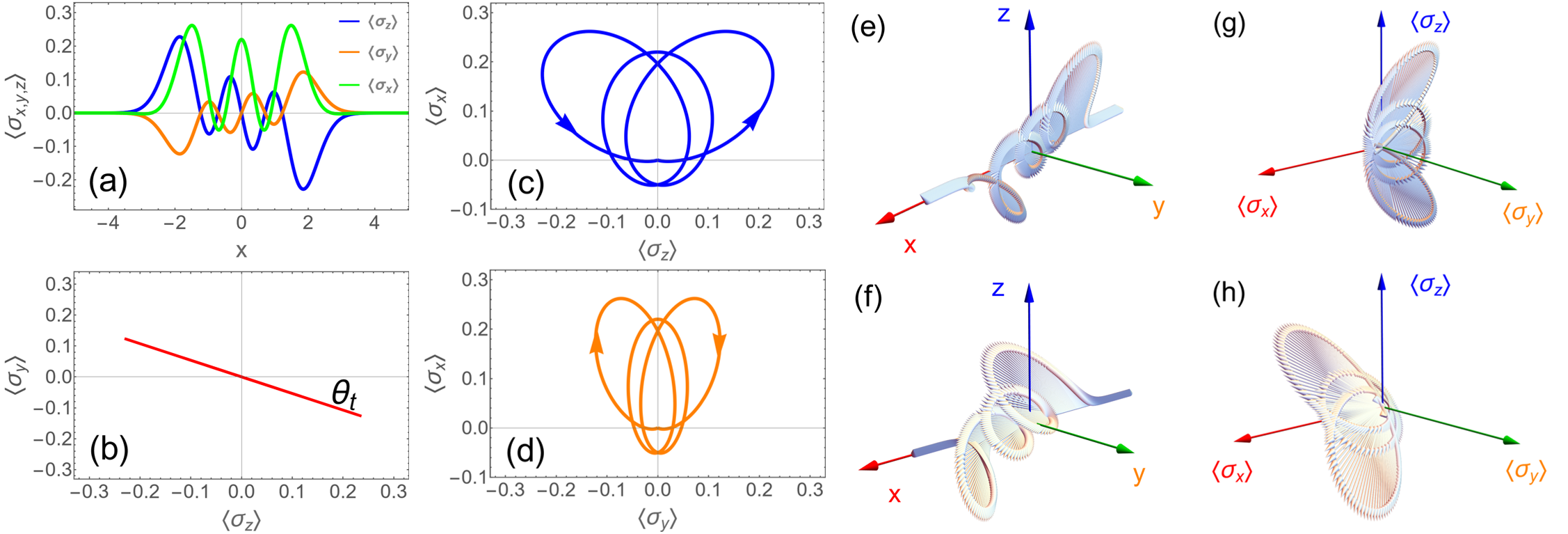
Figure 1: Spin texture and spin winding with and without non-Hermiticity. a) Space dependence of $\langle\sigma_{x}\rangle$, $\langle\sigma_{y}\rangle$ and $\langle\sigma_{z}\rangle$. b) Spin projection in the $\langle\sigma_{z}\rangle$-$\langle\sigma_{y}\rangle$ plane and tilting angle $\theta_{\rm t}$ of the spin-winding plane. c) Spin winding in the $\langle\sigma_{z}\rangle$-$\langle\sigma_{x}\rangle$ plane. d) Spin winding in the $\langle\sigma_{y}\rangle$-$\langle\sigma_{x}\rangle$ plane. e) 3D Spin texture without non-Hermiticity. f) 3D Spin texture with non-Hermiticity. g) 3D Spin winding without non-Hermiticity. h) 3D Spin texture with non-Hermiticity. Here in all panels $g=0.1g_{\rm s}$, $\omega=0.9$, $n=3$, $\eta=-1$, with $\Omega=1$ as the unit. The non-Hermiticity parameters $\kappa=0.5$, $\gamma=0.2$, $\Gamma=0.1$ in (a-d,f,h), while $\kappa=\gamma=\Gamma=0$ in (e,g).

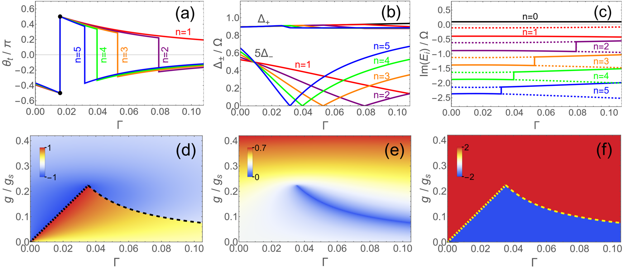
Figure 2: Reversal transitions of tilting angle and spin-winding direction with gap closing and without gap closing. a-c) Tilting angle $\theta_{\rm t}$ (a), energy gap $\Delta_{\pm}$ and imaginary part of $E_{i}$ versus $\Gamma$ at fixed $g=0.1g_{\rm s}$. d-f) The scaled tilting angle $\theta_{\rm t}/(\pi/2)$ (d), the smaller gap $\Delta_{-}$ plotted by $\Delta_{-}^{1/2}$ (e) and the spin winding number $n_{\rm w}^{zx}$ (f) in the $\Gamma$-$g$ plane. Here in all panels $\eta=-1$, $\kappa=0.5$, $\gamma=0.2$, $\omega=0.9$, with $\Omega=1$ as the unit. $n=1,2,3,4,5$ in (a-c) and $n=2$ in (d-f). The dotted lines and the dashed lines in (d,f) are analytic $g_{\rm R}$ and $g_{\rm GR}$ in (51) and (56).

Corresponding to the Hamitonian (3), the eigenstate in (5) can be represented as eigen wave function in the position space

$$\psi_{+}^{x}\left(x\right) \equiv \psi_{n,\Uparrow}^{\left(x,\eta\right)}\left(x\right)=C_{n\Uparrow}^{\left(\eta\right)}\phi_{n-1}\left(x\right)/\sqrt{N_{n}^{(\eta)}},$$ (11)

$$\psi_{-}^{x}\left(x\right) \equiv \psi_{n,\Downarrow}^{\left(x,\eta\right)}\left(x\right)=C_{n\Downarrow}^{\left(\eta\right)}\phi_{n}\left(x\right)/\sqrt{N_{n}^{(\eta)}}.$$ (12)

where $\phi_{n}\left(x\right)=\langle x|n\rangle=\frac{1}{\pi^{1/4}\sqrt{2^{n}n!}}H_{n}\left(x\right)e^{-x^{2}/2}$ with the Hermite polynomial $H_{n}\left(x\right)$ is the eigen function of the quantum harmonic oscillator with quantum number $n.$ As afore-mentioned the spin notation in the Hamiltonian (1) and the eigen state (5) is on the spin-$\sigma_{x}$ basis denoted by $\Uparrow$ and $\Downarrow$, we can also transform onto the spin-$\sigma_{z}$ basis represented by $\uparrow$ and $\downarrow$, via the basis transformation

$$\left|\uparrow\right\rangle = \frac{\left|\Uparrow\right\rangle+\left|\Downarrow\right\rangle}{\sqrt{2}},\qquad\left|\downarrow\right\rangle=\frac{\left|\Uparrow\right\rangle-\left|\Downarrow\right\rangle}{\sqrt{2}},$$ (13)

$$\left|\Uparrow\right\rangle = \frac{\left|\uparrow\right\rangle+\left|\downarrow\right\rangle}{\sqrt{2}},\qquad\left|\Downarrow\right\rangle=\frac{\left|\uparrow\right\rangle-\left|\downarrow\right\rangle}{\sqrt{2}}.$$ (14)

On the $\sigma_{z}$ basis the eigen wave function becomes

$$\psi_{n}^{\left(z,\eta\right)}=\ \psi_{+}^{z}\left(x\right)\left|\uparrow\right\rangle+\psi_{-}^{z}\left(x\right)\left|\downarrow\right\rangle$$ (15)

with the spin components

$$\psi_{+}^{z}\left(x\right) \equiv \psi_{n,\uparrow}^{\left(z,\eta\right)}\left(x\right)=\frac{C_{n\Uparrow}^{\left(\eta\right)}\phi_{n-1}\left(x\right)+C_{n\Downarrow}^{\left(\eta\right)}\phi_{n}\left(x\right)}{\sqrt{2N_{n}^{(\eta)}}},$$ (16)

$$\psi_{-}^{z}\left(x\right) \equiv \psi_{n,\downarrow}^{\left(z,\eta\right)}\left(x\right)=\frac{C_{n\Uparrow}^{\left(\eta\right)}\phi_{n-1}\left(x\right)-C_{n\Downarrow}^{\left(\eta\right)}\phi_{n}\left(x\right)}{\sqrt{2N_{n}^{(\eta)}}}.$$ (17)

From the above spin components of the eigen wave function on the $\sigma_{x}$ and $\sigma_{z}$ bases, we can determine the spin texture by

$$\langle\sigma_{z}\left(x\right)\rangle = \left|\psi_{+}^{z}\left(x\right)\right|^{2}-\left|\psi_{-}^{z}\left(x\right)\right|^{2}$$ (18)

$$\langle\sigma_{x}\left(x\right)\rangle = \left|\psi_{+}^{x}\left(x\right)\right|^{2}-\left|\psi_{-}^{x}\left(x\right)\right|^{2},$$ (19)

$$\langle\sigma_{y}\left(x\right)\rangle = i\left[\psi_{-}^{z}\left(x\right)^{\ast}\psi_{+}^{z}\left(x\right)-\psi_{+}^{z}\left(x\right)^{\ast}\psi_{-}^{z}\left(x\right)\right].$$ (20)

Note that the non-Hermitian model $H$ also possesses the parity symmetry as the Hermitian case, i.e. the parity operator $\hat{P}=\sigma_{x}\left(-1\right)^{a^{\dagger}a}$ commutes with the Hamiltonian, $[\hat{P},H]=0$ even in the presence of non-Hermiticity. An eigenstate has a negative parity when $n$ is even, while the parity is positive for odd $n$:

$$\hat{P}\psi_{n}^{\left(x,\eta\right)}=\left(-1\right)^{n-1}\psi_{n}^{\left(x,\eta\right)},\quad\hat{P}\psi_{0}=\left(-1\right)\psi_{0},$$ (21)

as $\left(-1\right)^{a^{\dagger}a}$ of $\hat{P}$ in the position representation inverses the space: $x\rightarrow-x$.Ying2020-nonlinear-bias On the $\sigma_{z}$ basis the parity involves both spin reversal and space inversion

$$\psi_{n,\uparrow}^{\left(z,\eta\right)}\left(x\right)=\left(-1\right)^{n-1}\psi_{n,\downarrow}^{\left(z,\eta\right)}\left(-x\right).$$ (22)

The parity symmetry of the eigen wave function leads to symmetric and anti-symmetric properties of spin texture:

$$\langle\sigma_{x}\left(-x\right)\rangle = \langle\sigma_{x}\left(x\right)\rangle,$$ (23)

$$\langle\sigma_{z}\left(-x\right)\rangle = -\langle\sigma_{z}\left(x\right)\rangle,$$ (24)

$$\langle\sigma_{y}\left(-x\right)\rangle = -\langle\sigma_{y}\left(x\right)\rangle,$$ (25)

which actually guarantee the close form of spin winding to form the topological feature, as will be discussed in Section VI.

We can decompose the wave-function coefficients into real and imaginary parts

$$C_{n\Uparrow}^{\left(\eta,\mathop{\rm Re}\right)} = \frac{1}{2}\left(\Omega-\omega\right)+\eta R\cos\frac{\vartheta}{2},$$ (26)

$$C_{n\Uparrow}^{\left(\eta,\mathop{\rm Im}\right)} = \frac{1}{2}\left(\kappa-\gamma\right)+\eta R\sin\frac{\vartheta}{2},$$ (27)

$$C_{n\Downarrow}^{\left(\eta,\mathop{\rm Re}\right)} = g\sqrt{n},\qquad C_{n\Downarrow}^{\left(\eta,\mathop{\rm Im}\right)}=-\Gamma\sqrt{n},$$ (28)

where

$$R = \left(A^{2}+B^{2}\right)^{1/4},\quad\vartheta=\arg\left(A-iB\right),$$ (29)

$$A = n\ \left(g^{2}-\Gamma^{2}\right)+\frac{1}{4}d_{\Omega\omega}^{2}-\frac{1}{4}d_{\kappa\gamma}^{2},$$ (30)

$$B = 2n\ g\ \Gamma-\frac{1}{2}d_{\kappa\gamma}d_{\Omega\omega},$$ (31)

with $d_{\kappa\gamma}=\kappa-\gamma$, $d_{\Omega\omega}=\Omega-\omega$. Thus the spin texture for state $\psi_{n}^{\left(x,\eta\right)}$ can be analytically obtained to be

$$\langle\sigma_{z}\left(x\right)\rangle=\frac{e^{-x^{2}}\ \widetilde{C}_{z}}{2^{n-3/2}\widetilde{N}_{\sigma}}H_{n-1}\left(x\right)H_{n}\left(x\right),$$ (32)

$$\langle\sigma_{x}\left(x\right)\rangle=\frac{e^{-x^{2}}}{2^{n}\widetilde{N}_{\sigma}}[\widetilde{D}_{x}H_{n-1}\left(x\right)^{2}-2\left(g^{2}+\Gamma^{2}\right)H_{n}\left(x\right)^{2}],$$ (33)

$$\langle\sigma_{y}\left(x\right)\rangle=\frac{e^{-x^{2}}\ \widetilde{C}_{y}}{2^{n-3/2}\widetilde{N}_{\sigma}}H_{n-1}\left(x\right)H_{n}\left(x\right),$$ (34)

where the coefficients before the Hermite polynomials are defined as

$$\widetilde{C}_{z} = gd_{\Omega\omega}-\Gamma d_{\kappa\gamma}+2\eta R(g\cos\frac{\vartheta}{2}-\Gamma\sin\frac{\vartheta}{2}),$$ (35)

$$\widetilde{C}_{y} = \Gamma d_{\Omega\omega}+gd_{\kappa\gamma}+2\eta R(\Gamma\cos\frac{\vartheta}{2}+g\sin\frac{\vartheta}{2}),$$ (36)

$$\widetilde{D}_{x} = d_{\Omega\omega}^{2}+d_{\kappa\gamma}^{2}+4R^{2}+4\eta R[d_{\Omega\omega}\cos\frac{\vartheta}{2}+d_{\kappa\gamma}\sin\frac{\vartheta}{2}],$$ (37)

and $\widetilde{N}_{\sigma}=\sqrt{\pi}(n-1)!\ 2N_{n}^{\left(\eta\right)}$. In the conventional Hermitian JCM, we have $\kappa=\gamma=\Gamma=0,B=0$ and $\vartheta=0$, which lead to $\langle\sigma_{x}\left(x\right)\rangle=0$.Ying-JC-winding In contrast, we now have a finite $\langle\sigma_{y}\left(x\right)\rangle$ contribution in the presence of the non-Hermiticity, which induces an out-of-plane component apart from the spin winding in the $\langle\sigma_{z}\left(x\right)\rangle$-$\langle\sigma_{x}\left(x\right)\rangle$ plane as will be discussed in more detail in Section VI. For state $\psi_{0}$, we have $\langle\sigma_{z}\left(x\right)\rangle=\langle\sigma_{y}\left(x\right)\rangle=0$ and $\langle\sigma_{x}\left(x\right)\rangle=-e^{-x^{2}}/\sqrt{\pi}$.

V Invariant Nodes in Spin Texture

An illustration of the spin texture is given in Figure 1a for $\langle\sigma_{x}\left(x\right)\rangle$ (green), $\langle\sigma_{y}\left(x\right)\rangle$ (orange) and $\langle\sigma_{z}\left(x\right)\rangle$ (blue). One sees that the spin texture has some oscillations which give rises to some nodes $x_{Z,i}^{\alpha}$ where $\langle\sigma_{\alpha}\left(x_{Z,i}^{\alpha}\right)\rangle=0$ for $\alpha\in\{x,y,z\}$. It has been noticed that the situation of nodes forms a topological feature that characterizes the topological phases in light-matter interaction.Ying-2021-AQT ; Ying-gapped-top ; Ying-Stark-top ; Ying-Spin-Winding ; Ying-JC-winding With a fixed node number one cannot go to another node state by continuous shape deformation, just as one cannot change a torus into a sphere by a continuous deformation in the topological picture of so-called rubber-sheet geometry. It has also been found that nodes have a correspondence to spin winding Ying-Spin-Winding ; Ying-JC-winding which is a more physical topological feature. The node sorting can algebraically decode the topological information encoded geometrically in the wave functions and spin windings.Ying-Spin-Winding Before addressing the spin winding in next section, here it is worthwhile to mention the invariant nodes in the spin texture. Indeed, Equations (32) and (34) indicate that the nodes of $\langle\sigma_{z}\left(x\right)\rangle$ and $\langle\sigma_{y}\left(x\right)\rangle$ are the roots of the Hermite polynomials which are independent of the system parameters. There are $2n$ nodes in $\langle\sigma_{x}\left(x\right)\rangle$ and $2n-1$ nodes in $\langle\sigma_{z}\left(x\right)\rangle$ and $\langle\sigma_{y}\left(x\right)\rangle$ according to the Hermite polynomials they contain. Involving the same Hermite polynomial factors $H_{n-1}\left(x\right)\$and $H_{n}\left(x\right)$, $\langle\sigma_{z}\left(x\right)\rangle$ and $\langle\sigma_{y}\left(x\right)\rangle$ share the same nodes. Moreover, they are invariant not only in the numbers but also in the positions, which may much reduce the experimental cost and simplify the identification of the topological states in experimental simulations, while usually in condensed matter one needs measurements over a global space to exactly identify the topological state MajoranaExpScience-2014 ; MajoranaExpScience-2017 ; ChernNumberExpPRL-2021 ; TopCriterion as topological feature is a global property rather than a local order parameter in the traditional phase transitions. Here, we see that the invariant nodes are unaffected by the non-Hermiticity.

VI Spin Winding

The spin texture is unfolded in the position space, while it manifests itself to be spin winding in spin expectation planes. In Figure 1b,c, the evolution of local spin expectation forms winding around the origin with a close form in the $\langle\sigma_{z}\left(x\right)\rangle$-$\langle\sigma_{x}\left(x\right)\rangle$ plane (panel (c)) and the $\langle\sigma_{y}\left(x\right)\rangle$-$\langle\sigma_{x}\left(x\right)\rangle$ plane (panel (d)). Such a close form of spin winding is guaranteed by the parity symmetry, as mentioned in Section IV. The two key factors to characterize the spin winding are the spin winding number and the winding direction, which we shall figure out explicitly in this section.

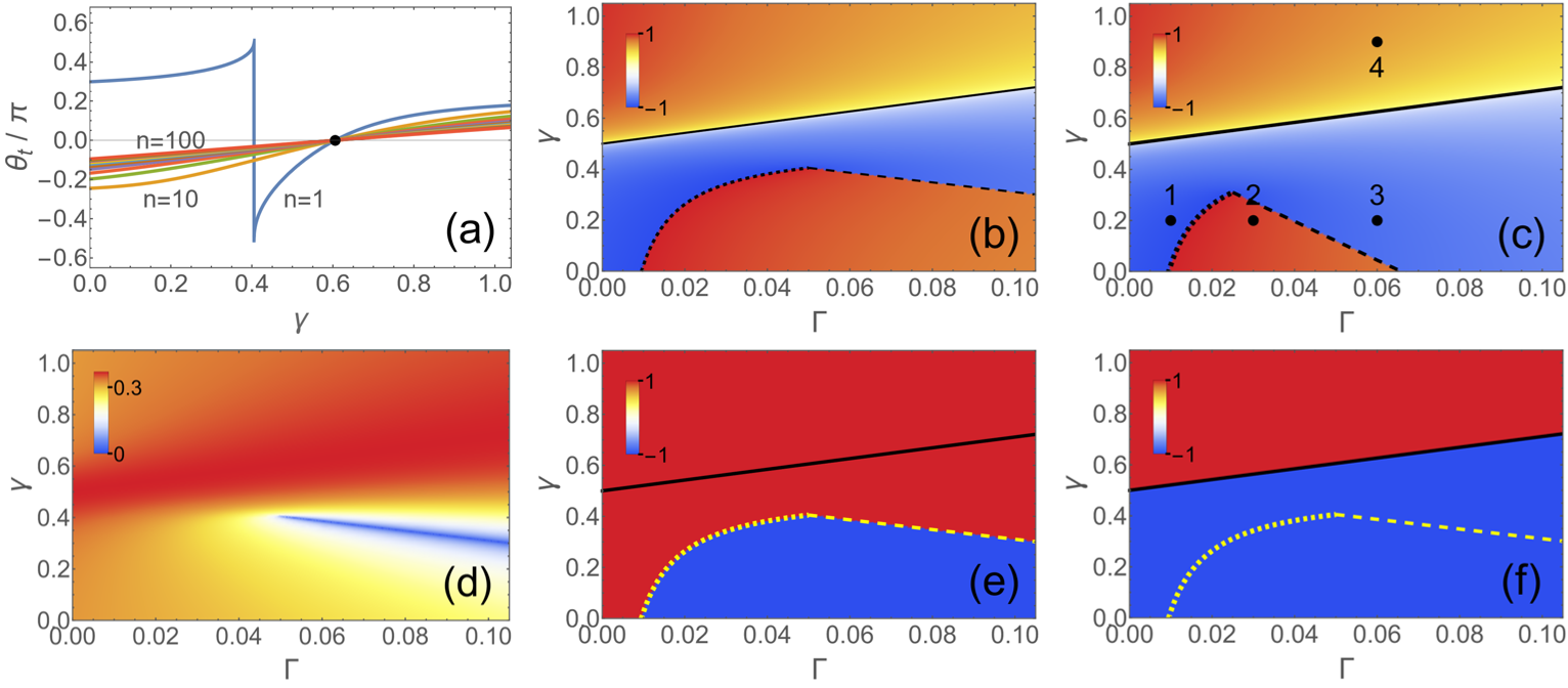
Figure 3: Super-invariant point for un-induced spin tilting by non-Hermiticity and for all energy levels. a) Spin tilting angle $\theta_{\rm t}$ versus $\gamma$ for different levels (every 10 levels plotted up to $n=100$) at fixed $\Gamma=0.05$. The dot marks the super-invariant point. b-f) $\theta_{\rm t}$ plotted by $(2\theta_{\rm t}/\pi)^{1/4}$ (b,c), $\Delta_{-}^{1/2}$ (d), $n^{zx}_{\rm w}$ (e) and $n^{yx}_{\rm w}$ (f) in the $\Gamma$-$\gamma$ plane. Here in all panels $\eta=-1$, $\kappa=0.5$, $g=0.1g_{\rm s}$ and $\omega=0.9$, with $\Omega=1$ as the unit. $\gamma=0.05$ in (a), $n=1$ in (b,d-f) and $n=4$ in (c). The the dashed lines, dotted lines and solid lines in (b,c,e,f) are analytic $\gamma_{\rm R}$ and $\gamma_{\rm GR}$ in (52) (57) and (59). The dots in (c) mark some representative points for the plots of spin winding direction in Figure 4.

Figure 4: Winding direction reversals: Spin winding in the $\langle\sigma_{z}\left(x\right)\rangle$-$\langle\sigma_{x}\left(x\right)\rangle$ plane (a-d) and the $\langle\sigma_{y}\left(x\right)\rangle$-$\langle\sigma_{x}\left(x\right)\rangle$ plane (e-h), respectively before the reversal transition (a,e), after the reversal transition and before the gapped reversal transition (b,f), after the gapped reversal transition (c,g) and beyond the super-invariant point (d,h), corresponding to the dots marked by $1,2,3,4$ as representative points of the phases in Figure 3c. a,e) $\Gamma=0.01$ and $\gamma=0.2$; b,f) $\Gamma=0.03$ and $\gamma=0.2$; c,g) $\Gamma=0.06$ and $\gamma=0.2$; d,h) $\Gamma=0.06$ and $\gamma=0.9$. Here in all panels $n=4$, $\eta=-1$, $\kappa=0.5$, $\gamma=0.2$, $\omega=0.9$, $g=0.1g_{\rm s}$ with $\Omega=1$ as the unit. The spin amplitudes are plotted by $|\langle\sigma_{\alpha}\left(x\right)\rangle|^{1/2}$ for all components $\alpha=x,y,z$ to amplify the detail. The spin winding direction is indicated by the arrows, and also represented by the color with blue for counter-clockwise and orange for clockwise.

VI.1 Spin Winding Number

The spin winding number in the $\langle\sigma_{\alpha}\left(x\right)\rangle$-$\langle\sigma_{\beta}\left(x\right)\rangle$ plane, where $\alpha,\beta\in\{x,y,z\},$ is defined by

$$n_{{\rm w}}^{\alpha\beta}=\frac{1}{2\pi}\int_{-\infty}^{\infty}\frac{\langle\sigma_{\alpha}\left(x\right)\rangle\partial_{x}\langle\sigma_{\beta}\left(x\right)\rangle-\langle\sigma_{\beta}\left(x\right)\rangle\partial_{x}\langle\sigma_{\alpha}\left(x\right)\rangle}{\langle\sigma_{\alpha}\left(x\right)\rangle^{2}+\langle\sigma_{\beta}\left(x\right)\rangle^{2}}dx,$$ (38)

which has also been applied in topological classification in nanowire systems and quantum systems with geometric driving.Ying2016Ellipse ; Ying2017EllipseSC ; Ying2020PRR ; Gentile2022NatElec Although Equation (38) involves calculus of both integral and differential which is numerically more difficult to treat, it was pointed out that the winding number can be extracted algebraically in terms of the nodes without integral or differential.Ying-Spin-Winding ; Ying-JC-winding Indeed, by assuming $M_{\alpha}$ number of $\langle\sigma_{\alpha}\left(x\right)\rangle$ nodes at finite node position $x_{Z,i}^{\alpha}$, it has been rigorously provenYing-JC-winding that the spin winding number defined by the involved geometric integral (38) is equal to the simple algebraic sum of spin signs at nodes

$$n_{{\rm w}}^{\alpha\beta} = -\sum_{i=0}^{M_{\beta}}\frac{sgn\langle\sigma_{\alpha}(x_{Z,i+1}^{\beta})\rangle-sgn\langle\sigma_{\alpha}(x_{Z,i}^{\beta})\rangle}{4\eta_{\beta}\left(i\right)}$$ (39)

$$= \sum_{i=0}^{M_{\alpha}}\frac{sgn\langle\sigma_{\beta}(x_{Z,i+1}^{\alpha})\rangle-sgn\langle\sigma_{\beta}(x_{Z,i}^{\alpha})\rangle}{4\eta_{\alpha}\left(i\right)}$$ (40)

which holds for a generic spin winding. Here $\eta_{\alpha}\left(i\right)$ is the sign of $\langle\sigma_{\alpha}\left(x\right)\rangle$ in space section $x\in(x_{Z,i}^{\alpha},x_{Z,i+1}^{\alpha}).$ The edge sections $i=0,M_{\alpha}$ are $(-\infty,x_{Z,1}^{\alpha})$ and $(x_{Z,M_{\alpha}}^{\alpha},\infty)$ by setting $x_{Z,0}^{\alpha}=-\infty$ and $x_{Z,M_{\alpha}+1}^{\alpha}=\infty$. For the nodes $sgn\langle\sigma_{\alpha}\rangle={\rm sign}\langle\sigma_{\alpha}\rangle,$ while for the infinity ends $sgn\langle\sigma_{\alpha}\rangle=2\arcsin\langle\overline{\sigma}_{\alpha}\rangle/\pi$ where $\langle\overline{\sigma}_{\alpha}\rangle=\langle\sigma_{\alpha}\rangle/\sqrt{\langle\sigma_{\alpha}\rangle^{2}+\langle\sigma_{\beta}\rangle^{2}}$. Despite $M_{x}\neq M_{z},$ Equations (39) and (40) are equal as $M_{x}=2n$ with $sgn\langle\sigma_{z,y}(\pm\infty)\rangle=0$ while $M_{z,y}=2n-1$ but with $\left|sgn\langle\sigma_{x}(\pm\infty)\rangle\right|=1$. The difference of $sgn\langle\sigma_{z,y}(\pm\infty)\rangle$ and $\left|sgn\langle\sigma_{x}(\pm\infty)\rangle\right|$ comes from the ratio limit $\frac{\langle\sigma_{z,y}\left(x\right)\rangle}{\langle\sigma_{x}\left(x\right)\rangle}|_{x\rightarrow\pm\infty}\rightarrow 0$ as $\langle\sigma_{x}\left(x\right)\rangle$ contains a $H_{n}\left(x\right)^{2}$ term which is in a higher rank of polynomial than $H_{n-1}\left(x\right)H_{n}\left(x\right)$ in $\langle\sigma_{z,y}\left(x\right)\rangle.$

As all the $\langle\sigma_{\alpha}\rangle$ components in (32)-(34) only involve neighboring Hermite polynomials, the spin is winding in one direction without anti-winding nodes or returning knots,Ying-JC-winding $\eta_{\alpha}\left(i\right)$ changes the sign alternatively and brings all the nodes into full contributions. Thus, we have the absolute spin winding numbers in the $\langle\sigma_{z}\left(x\right)\rangle$-$\langle\sigma_{x}\left(x\right)\rangle$ plane and the $\langle\sigma_{y}\left(x\right)\rangle$-$\langle\sigma_{x}\left(x\right)\rangle$ plane both equal to the excitation number

$$\left|n_{{\rm w}}^{zx}\right|=\left|n_{{\rm w}}^{yx}\right|=n$$ (41)

for the eigen state. Thus the excitation number $n$ is now endowed the topological connotation to be the topological quantum number of spin winding not only in the conventional Hermitian JCM but also in the general non-Hermitian JCM.

VI.2 Spin Winding Direction

Besides the winding-number magnitude, the spin winding direction is also an important quantum character. Since the spin winding has no returning within an eigen state,Ying-JC-winding the winding direction can be conveniently figured out from the ratio sign of $\langle\sigma_{z,y}\left(x\right)\rangle$ and $\langle\sigma_{x}\left(x\right)\rangle$ at infinity where the winding starts. Actually the winding will be clockwise when it starts in the 1st or 3rd quadrant of the $\langle\sigma_{z,y}\left(x\right)\rangle$-$\langle\sigma_{x}\left(x\right)\rangle$ plane, as a counter-clockwise winding would spuriously generate a $2n+1$ umber of $\langle\sigma_{z,y}\left(x\right)\rangle$ nodes exceeding the correct node number; Otherwise in the 1st or 3rd quadrant, the winding is counter-clockwise. Thus, the spin winding is counter-clockwise (clockwise) if the sign of

$$s_{{\rm w}}^{zx} = \rm{sign}\frac{\langle\sigma_{z}\left(x\right)\rangle}{\langle\sigma_{x}\left(x\right)\rangle}|_{x\rightarrow-\infty}=\rm{sign}(\widetilde{C}_{z}),$$ (42)

$$s_{{\rm w}}^{yx} = \rm{sign}\frac{\langle\sigma_{y}\left(x\right)\rangle}{\langle\sigma_{x}\left(x\right)\rangle}|_{x\rightarrow-\infty}=\rm{sign}(\widetilde{C}_{y}),$$ (43)

is negative (positive). Here we have taken into account the property $H_{n-1}\left(x\right)H_{n}\left(x\right)<0$ at $x\rightarrow-\infty$ due to $H_{n}\left(x\right)\propto x^{n}$ there in the leading order. Finally, the complete information of the spin winding number includes the magnitude $n$ counting the winding rounds and the sign representing the winding direction:

$$n_{{\rm w}}^{zx} = -s_{{\rm w}}^{zx}n,$$ (44)

$$n_{{\rm w}}^{yx} = -s_{{\rm w}}^{yx}n,$$ (45)

which defines positive $n_{{\rm w}}^{\alpha\beta}$ for counter-clockwise winding and negative for clockwise according to (38).

In the conventional Hermitian JCM,

$$\widetilde{C}_{z}\rightarrow g\left(\Omega-\omega\right)+\eta g\sqrt{\left(\Omega-\omega\right)^{2}+4g^{2}n},$$ (46)

which indicates that all states with $\eta=-1$ have a counter-clockwise spin winding direction, while the winding direction of the states with $\eta=+1$ is opposite. However, such a unified picture of the winding direction is broken in the presence of non-Hermiticity, as we shall address in Sections VIII-X.

VII Tilting Angle of Spin Winding Plane

We have seen below (35) that there is no $\langle\sigma_{y}\left(x\right)\rangle$ component in the conventional Hermitian JCM. A finite $\langle\sigma_{y}\left(x\right)\rangle$ component emerges in the presence of the non-Hermiticity. Equations (32)-(34) shows that $\langle\sigma_{y}\left(x\right)\rangle$ is proportional to $\langle\sigma_{z}\left(x\right)\rangle$ and has the same the magnitude of spin winding number, which means that the non-Hermiticity only tilts the spin winding plane while the topological feature is maintained. This is more clearly demonstrated by Figure 1b where the spin winding in the $\langle\sigma_{z}\left(x\right)\rangle$-$\langle\sigma_{y}\left(x\right)\rangle$ plane is completely flat. The zero tilting of the spin winding plane in the Hermitian case and finite tilting in the non-Hermitian case can be further visualized in Figure 1e-h by the 3D plots of the spin texture (e,f) and spin winding (g,h), with the comparison of the Hermitian case (e,g) and the non-Hermitian case (f,h). The tilting degree can be described by the ratio

$$R_{yz}=\frac{\langle\sigma_{y}\left(x\right)\rangle}{\langle\sigma_{z}\left(x\right)\rangle}=\frac{\widetilde{C}_{y}}{\widetilde{C}_{z}}=\tan\theta_{{\rm t}}$$ (47)

which is exactly the same at any position $x$. The tilting angle is then denoted by

$$\theta_{{\rm t}}=\arctan\frac{\widetilde{C}_{y}}{\widetilde{C}_{z}}.$$ (48)

The tilting angle $\theta_{{\rm t}}$ not only describes the tilting degree but also can help to track and reveal some winding reversal transitions and super-invariant points, as unveiled in the following sections.

VIII Fractional Phase Gain and Reversal Transition of Spin Winding at Gap Closing

We find a reversal transition of the spin winding induced by the non-Hermiticity, with the reversal both in the tilting angle of the spin winding plane and the direction of the spin winding. An example is illustrated in Figure 2a, where one finds a jump or a reversal of the tilting angle $\theta_{{\rm t}}$ in varying a non-Hermiticity parameter such as $\Gamma$. Such a reversal transition occurs for all excited levels with level-dependent transition point. The $\theta_{{\rm t}}$ jump originates from the square root term in (7), $S_{r}=\sqrt{e_{-}^{2}+n\ \widetilde{g}^{2}}=\sqrt{A-iB}$ with $B$ in (31) induced by the non-Hermiticity. Under a negative $A$, when $B$ is crossing its zero point a shift from $\pi$ to $-\pi$ will take place for $\vartheta$ in (29). This $2\pi$ phase gain is trivial in usual case, but here inside the square root it will fractionally contribute a $\pi$ phase with a sign change of $S_{r}$, which happens to reverse the tilting angle of the spin winding plane (See the proof in Appendix A).

To see the situation of the reversal transition, we can decompose $E^{\left(n,\eta\right)}$ into real part and imaginary part

$$E_{\mathop{\rm Re}}^{\left(n,\eta\right)} = (n-\frac{1}{2})\omega+\eta R\cos\frac{\vartheta}{2},$$ (49)

$$E_{\mathop{\rm Im}}^{\left(n,\eta\right)} = -(n-\frac{1}{2})\kappa+\eta R\sin\frac{\vartheta}{2}.$$ (50)

The real part should represent the energy difference of the levels, while the imaginary part would decide the relaxation time to the steady state in dynamics.Plenio1998-quantum-jump ; NonHermitian-Nori2019 The $\theta_{{\rm t}}$ reversal transition occurs at gap closing of $E_{\mathop{\rm Re}}^{\left(n,\eta\right)}$, as shown by the smaller gap $\Delta_{-}=|E_{\mathop{\rm Re}}^{\left(n,+1\right)}-E_{\mathop{\rm Re}}^{\left(n,-1\right)}|$ in Figure 2b despite that the larger gap $\Delta_{+}$ between different-$n$ levels is finite. The gap closing stems from the $\eta R\cos\frac{\vartheta}{2}$ term of $E_{\mathop{\rm Re}}^{\left(n,\eta\right)}$, as $\cos\frac{\vartheta}{2}=0$ for $\vartheta=\pm\pi$ at the transition point. Across the transition there is indeed a phase shift as indicated by the imaginary part of $E^{\left(n,\eta\right)}$ in Figure 2c.

The transition boundary can be analytically found from $B=0$ to be

$$\kappa_{{\rm R}} = \gamma+\frac{4ng\Gamma}{\left(\Omega-\omega\right)},\qquad\Gamma_{{\rm R}}=\frac{\left(\kappa-\gamma\right)\left(\Omega-\omega\right)}{4ng},$$ (51)

$$\gamma_{{\rm R}} = \kappa-\frac{4ng\Gamma}{\left(\Omega-\omega\right)},\qquad g_{{\rm R}}=\frac{\left(\kappa-\gamma\right)\left(\Omega-\omega\right)}{4n\Gamma}.$$ (52)

Note, as afore-mentioned, that the transition occurs only under the condition of negative $A,$ which requires

$$n\ \left(g^{2}-\Gamma^{2}\right)+\frac{1}{4}d_{\Omega\omega}^{2}-\frac{1}{4}d_{\kappa\gamma}^{2}<0.$$ (53)

Here the condition (53) is imposed on the transition boundary. For example (53) becomes

$$\Gamma_{{\rm R}}^{2}>\Gamma_{{\rm A}}^{2}=g^{2}+\frac{1}{4n}\left[\left(\Omega-\omega\right)^{2}-\left(\kappa-\gamma\right)^{2}\right]$$ (54)

which means that one always has the transition in varying $\Gamma$ if the other parameters lead to $\Gamma_{{\rm A}}^{2}<0$, otherwise for $\Gamma_{{\rm A}}^{2}>0$ the existence of the reversal transition requires

$$\Gamma>\Gamma_{{\rm R}}^{\min}\equiv\frac{\left|\Omega-\omega\right|}{2\sqrt{n}}\quad\text{and}\quad\left(\kappa-\gamma\right)\left(\Omega-\omega\right)>0$$ (55)

where $\Gamma$ is supposed to be positive.

In Figure 2d-f we provide the maps in the $\Gamma$-$g$ plane for the spin tilting angle $\theta_{{\rm t}}$ (d), the smaller gap $\Delta_{-}$ (d) and the spin winding number $n_{{\rm w}}^{zx}$ (f). The dashed lines in panels (d) and (f) are the analytic result from (51) and (52). One sees that there is a $\theta_{{\rm t}}$-jump across this boundary and the gap is closing (blue belt in panel (e)). One may also notice that, besides the reversal of $\theta_{{\rm t}}$ in panel (d), there is also a reversal of the spin winding direction in panel (e) at the transition boundary. We shall demonstrate in Section XI the winding direction reversal more explicitly by the spin winding itself after extracting other transitions.

Figure 5: 3D transition boundaries for the spin winding reversal transition (red), gapped reversal transition (yellow) and super-invariant point (blue) in $\kappa$-$\Gamma$-$\gamma$ (a), $\Gamma$-$g$-$\kappa$ (b), $\Gamma$-$g$-$\gamma$ (c) and $\gamma$-$g$-$\kappa$ (d) spaces. a) $g=0.1g_{\rm s}$, b) $\gamma=0.3$, c) $\kappa=0.5$, d) $\Gamma=0.1$. In all panels, $\omega=0.9$, $n=1$ and $\eta=-1$, with $\Omega=1$ as the unit. The reversal transition is $n$-dependent while the other two transitions are level-independent.

IX Reversal Transition of Spin Winding without Gap Closing

The reversal transitions in Section VIII occur at gap closing, in this section we shall reveal another reversal transition without gap closing. Moreover, this new transition is partially level-independent in the sense that the transition point is the same for all the levels that possess this transition (Here by “partially level-independent” we mean that this transition may vanish after meeting the first reversal transition in Section VIII). Indeed in Figure 2a all the lines of tilting angle $\theta_{{\rm t}}$ with different $n$ meet at the same point marked by the dots around $\Gamma=0.016\Omega$ where there is an angle reversal from $\theta_{{\rm t}}=-\pi/2$ to $\pi/2$. Note here there is no gap closing as one can see in Figure 2b, in contrast to the vanishing gap at the other reversal transitions.

This gapped reversal (GR) transition appears when $\langle\sigma_{z}\left(x\right)\rangle$ overall at any position $x$ is going through its zero point, which can be realized at $\widetilde{C}_{z}=0$ in (35) with the analytic critical point

$$\kappa_{{\rm GR}} = \gamma+g\frac{\left(\Omega-\omega\right)}{\Gamma},\qquad\Gamma_{{\rm GR}}=g\frac{\left(\Omega-\omega\right)}{\left(\kappa-\gamma\right)},$$ (56)

$$\gamma_{{\rm GR}} = \kappa-g\frac{\left(\Omega-\omega\right)}{\Gamma},\qquad g_{{\rm GR}}=\Gamma\frac{\left(\kappa-\gamma\right)}{\left(\Omega-\omega\right)}.$$ (57)

In Figure 2d,f, the dotted lines are plotted by the analytic expressions for the gapped reversal transition in (57), which reproduces the boundary manifested by $\theta_{t}$ and $n_{\rm w}^{zx}$. Correspondingly in Figure 2e, there is no gap closing, in contrast to the gap closing in the blue belt around $g_{{\rm R}}$. Also, besides the reversal of the tilting angle of the spin winding plane, there is a reversal of spin winding direction in the $\langle\sigma_{z}\left(x\right)\rangle$-$\langle\sigma_{x}\left(x\right)\rangle$ plane as indicated by the sign changeover of $n_{{\rm w}}^{zx}$ in Figure 2f.

X Super-Invariant Point: No Spin Tilting, Level-Independent, and Without Gap Closing.

We find a super-invariant point in the presence of non-Hermiticity, in the sense that it not only has no tilting of the spin winding plane, as the Hermitian case, but also is independent of $n$. We give an illustration in Figure 3a where all $\theta_{{\rm t}}$ lines with different $n$ go through a same point with $\theta_{{\rm t}}=0$ in the variation of $\gamma$, which forms a super-invariant point as marked by the black dot. The super-invariant point can be seen in Figure 3b,c in the $\Gamma$-$\gamma$ plane where the invariant point becomes a line (solid black) which remains the same when we change the levels ($n=1$ in panel (b) and $n=4$ (c)), Here, by the way, the dotted lines in (b) and (c) confirm the gapped reversal transition in Section IX which is also level-independent, while the dashed lines denoting the reversal transitions in Section VIII are level dependent. There is no spin winding direction reversal in the $\langle\sigma_{z}\left(x\right)\rangle$-$\langle\sigma_{x}\left(x\right)\rangle$ plane, as shown by $n_{{\rm w}}^{zx}$ in Figure 3e where $n_{{\rm w}}^{zx}$ is changing the sign only at the $\gamma_{{\rm GR}}$ boundary (dotted) and the $\gamma_{{\rm R}}$ boundary (dashed) but not at the super-invariant boundary. Although there is a spin winding direction reversal in the $\langle\sigma_{y}\left(x\right)\rangle$-$\langle\sigma_{x}\left(x\right)\rangle$ plane, the tilting angle is changing slowly rather than an abrupt jump, as one can see in Figure 3a. Here the seemingly fast change of $\theta_{{\rm t}}$ around the solid lines in Figure 3b,c is due to the plot in amplitude amplifying by $\left|\theta_{{\rm t}}\right|^{1/4}$ to increase the color contrast and visibility of the super-invariant boundary.

The no-tilting condition can be provided by setting $\widetilde{C}_{y}=0,$ from which we obtain the analytic super-invariant point

$$\kappa_{{\rm SI}} = \gamma-\frac{\Gamma\left(\Omega-\omega\right)}{g},\qquad\Gamma_{{\rm SI}}=\frac{g\left(\gamma-\kappa\right)\ }{\left(\Omega-\omega\right)},$$ (58)

$$\gamma_{{\rm SI}} = \kappa+\frac{\Gamma\left(\Omega-\omega\right)}{g},\qquad g_{{\rm SI}}=\frac{\Gamma\left(\Omega-\omega\right)}{\left(\gamma-\kappa\right)},$$ (59)

which is plotted in the solid lines and agrees with the overall $\theta_{{\rm t}}$ map in Figure 3b,c

XI Reversals of Spin Winding Direction around the Three Special Points

So far we have figured out the three special points of the reversal transition, the gapped reversal transition and the super invariant point. Although we have mentioned the reversal of spin winding direction for each point by the sign changeover in the spin winding number $n_{{\rm w}}^{zx}$ and $n_{{\rm w}}^{yx}$, it may provide a more definite and overall view by a straight demonstration of the spin winding itself for these special points together. Here in Figure 4 the spin windings in the $\langle\sigma_{z}\left(x\right)\rangle$-$\langle\sigma_{x}\left(x\right)\rangle$ plane (panels (a-d)) and the $\langle\sigma_{y}\left(x\right)\rangle$-$\langle\sigma_{x}\left(x\right)\rangle$ plane (panels (e-h)) are plotted for some representative points of the phases before and after the three special points, as marked by the dots in Figure 3c and labeled by the number $1,2,3,4,$ corresponding to panels (a,e), (b,f), (c,g), (d,g) in Figure 4. The reversal transition lies between points $1$ and $2$, the gapped reversal transition between $2$ and $3$, and the super invariant point between $3$ and $4$. Although the spin winding panels (a,b,d-f,h) has a shape in formal or spiritual similarity with a long or broad face in long hair and a mask while panels (c,g) look like a face of catgirl, they are topologically the same except for the spin winding number. Here the spin winding direction is not only marked by the arrows but also by the colors with blue for counter-clockwise direction and orange for clockwise direction. From Figure 4(a-c) we see clearly that there is a reversal of spin winding direction in the $\langle\sigma_{z}\left(x\right)\rangle$-$\langle\sigma_{x}\left(x\right)\rangle$ plane both for the reversal transition and the gapped reversal transition, but from panels (e-g) one finds no direction reversal in the $\langle\sigma_{y}\left(x\right)\rangle$-$\langle\sigma_{x}\left(x\right)\rangle$ plane; Conversely, from (c-d) there is no spin winding direction reversal for the super-invariant point in the $\langle\sigma_{z}\left(x\right)\rangle$-$\langle\sigma_{x}\left(x\right)\rangle$ panels (e-g) but from (g-h) there is a reversal in the $\langle\sigma_{y}\left(x\right)\rangle$-$\langle\sigma_{x}\left(x\right)\rangle$ plane.

XII 3D Boundaries

In Figures 2 and 3 only some 2D boundaries are plotted for the three special points as afore-discussed, to get a panorama here we give 3D boundaries. In Figure 5, we give some overview boundaries for the spin winding reversal transition (red), the gapped reversal transition (yellow) and the super-invariant point (blue) in the $\kappa$-$\Gamma$-$\gamma$, $\Gamma$-$g$-$\kappa$, $\Gamma$-$g$-$\gamma$ and $\gamma$-$g$-$\kappa$ dimensions respectively with a fixed $g$, $\gamma$, $\kappa$ and $\Gamma$. Basically, spin winding reversal transition and the gapped reversal transition will meet at some boundaries, as one sees in panels (a-c), while the super-invariant point is separate from them unless in the special situation with $\Gamma=0$ as in panels (b,c) where the super-invariant point may meet the reversal transition at $g=0$ and $\kappa=\gamma$. Another trend one can see is that the super-invariant point can arise earlier than the reversal transitions in varying $\kappa$, despite it appears later in varying $\gamma$. These overview pictures may be helpful in choosing parameters for manipulation of the three special points.

XIII Conclusions and Discussions

We have studied rigorously the topological feature of the fundamental JCM in the presence of general non-Hermiticity which may arise from the dissipation and decay rates of the coupling, the qubit and the bosonic field. We have found that the topological feature of the eigenstates are quite robust against the non-Hermiticity. Indeed, the non-Hermiticity only tilts the spin winding plane, while the spin texture nodes and the spin winding number, which characterize the topological feature, remain unaffected in the protection of parity symmetry.

Based on the exact solution of the JCM, we have analytically extracted the spin texture in the position space which forms the spin winding in the space of local spin expectation. In comparison with the conventional Hermitian JCM, of which the spin is winding only in the $\langle\sigma_{z}\left(x\right)\rangle$-$\langle\sigma_{x}\left(x\right)\rangle$ plane, the presence of the non-Hermiticity induces an additional winding component in the $\langle\sigma_{y}\left(x\right)\rangle$-$\langle\sigma_{x}\left(x\right)\rangle$ plane. We see that $\langle\sigma_{y}\left(x\right)\rangle$ is proportional to $\langle\sigma_{z}\left(x\right)\rangle$, which gives rise to a tilting angle of the total winding plane. The spin texture components $\langle\sigma_{y}\left(x\right)\rangle$ and $\langle\sigma_{z}\left(x\right)\rangle$ share the same nodes and the nodes are invariant in variations of system parameters, which is not only valid in the Hermitian case but also in the non-Hermitian situation. The spin winding number is shown to be equal to the excitation number both in the $\langle\sigma_{z}\left(x\right)\rangle$-$\langle\sigma_{x}\left(x\right)\rangle$ plane and the additional $\langle\sigma_{y}\left(x\right)\rangle$-$\langle\sigma_{x}\left(x\right)\rangle$ plane, which endows the excitation number a topological connotation as the topological quantum number in both winding planes.

Although the magnitude of spin winding number is unaffected by the non-Hermiticity, the winding direction may be reversed in non-Hermiticity. We first find a level-dependent reversal transition of the spin winding. The non-Hermiticity generates a fractional phase in the square root term of the eigen wave function, which leads to a jump or reversal of the spin tilting angle and a reversal of spin winding direction in the $\langle\sigma_{z}\left(x\right)\rangle$-$\langle\sigma_{x}\left(x\right)\rangle$ plane. The total jump of tilting angle is a fraction of $\pi$, with the degree of the fraction depending on the energy levels. Such reversal transition occurs at gap closing, similarly to the conventional topological phase transitions which require a gap closing as in condensed matterTopo-Wen ; Hasan2010-RMP-topo ; Yu2010ScienceHall ; Chen2019GapClosing ; TopCriterion ; Top-Guan ; TopNori and also in light-matter interactions.Ying-2021-AQT ; Ying-gapped-top ; Ying-Stark-top ; Ying-Spin-Winding

We also find a gapped reversal transition. This transition point is the same for all the energy levels that possess this transition, in contrast to the first reversal transition which is level-dependent. This gapped reversal transition involves a total jump of tilting angle by $\pi$ and is accompanied with a reversal of spin winding direction in the $\langle\sigma_{z}\left(x\right)\rangle$-$\langle\sigma_{x}\left(x\right)\rangle$ plane. In particular, unlike the first reversal transition, this transition occurs in a situation without gap closing, resembling the unconventional topological phase transitions which break the traditional condition of gap closing as in some special cases of condensed matterAmaricci-2015-no-gap-closing ; Xie-QAH-2021 and light-matter interactions.Ying-gapped-top ; Ying-Stark-top ; Ying-Spin-Winding

Finally we have also revealed a super-invariant point which has no titling angle as the Hermitian case despite in a finite non-Hermiticity. The super-invariant sense lies in the aspect that it is completely independent of the energy levels. Such a super-invariant point does not reverse the spin winding direction in the $\langle\sigma_{z}\left(x\right)\rangle$-$\langle\sigma_{x}\left(x\right)\rangle$ plane, although it varies the winding direction in the $\langle\sigma_{y}\left(x\right)\rangle$-$\langle\sigma_{x}\left(x\right)\rangle$ plane in a slow way instead of an abrupt jump as in the reversal transitions. The super-invariant point also occurs in the unconventional situation without gap closing.

The present work has focused on the robustness of the topological feature of all the eigenstates against the non-Hermiticity. In fact the non-Hermiticity will also influence the transitions in the ground statesYing-JC-winding and induce some new effects, which deserves a special discussion in some other work.Ying-JC-Non-Hermitian-Transition

As a final discussion it should be mentioned that the model can be implemented in realistic systems, such as in superconducting circuits and hybrid quantum systems,you024532 ; Yimin2018 ; NonHermitianJCM-2022SciChina with access to ultra-strong couplings possible Ulstrong-JC-1 ; Ulstrong-JC-3-Adam-2019 ; Ulstrong-JC-2 and the dissipation controllable NonHermitianJCM-2022SciChina . The position $x$ can be represented by the flux of Josephson junctions and the spin texture might be measured by interference devices and magnetometer.you024532 With these possible platforms, the found robust topological feature against the non-Hermiticity, including the invariant spin winding number and supper invariant points, may be favorable in practical applications where the dissipation and decay rates may be unnegligible. The reversal transitions indicate that one may in turn to utilize the disadvantageous dissipation and decay rates to reverse the spin winding direction, which should add a control way for topological manipulation of light-matter coupling systems. The gapped situation in the gapped reversal transition and supper invariant point also is favorable in making senors as the gapped situation could avoid the detrimental time divergent problem in preparing probe state.Ying2022-Metrology

As a closing remark, we speculate that our results may be also relevant for other systems as the JCM under consideration has the effective Rashba/Dresselhaus spin-orbit coupling which shares similarity with the coupling in nanowires Nagasawa2013Rings ; Ying2016Ellipse ; Ying2017EllipseSC ; Ying2020PRR ; Gentile2022NatElec , cold atoms Li2012PRL ; LinRashbaBECExp2011 and relativistic systems.Bermudez2007

Appendix A Proof for Reversal of $\theta_{{\rm t}}$ at $\Gamma_{{\rm R}}$

The reversal transition found in Section VIII occurs due to the $2\pi$ phase gain in the argument $\vartheta$ of the complex parameter $A-iB$ which leads to a nontrivial $\pi$ phase in the square root term $S_{r}$. This $\pi$ phase of $S_{r}$ would result in a jump of the tilting angle $\theta_{{\rm t}}$ to some $\theta_{{\rm t}}+\Delta\theta_{{\rm t}}$. Here we prove this tilting angle jump is actually an angle reversal from $\theta_{{\rm t}}$ to $-\theta_{{\rm t}}$. We can set $\vartheta\rightarrow\eta_{{\rm R}}\pi$ with $\eta_{{\rm R}}=\pm 1$ around the reversal transition, e.g. around $\Gamma_{{\rm R}}$ in varying $\Gamma$. Then

$$\widetilde{C}_{z}\rightarrow\widetilde{C}_{z1}+\eta_{{\rm R}}\widetilde{C}_{z2},\quad\widetilde{C}_{y}\rightarrow\widetilde{C}_{y1}+\eta_{{\rm R}}\widetilde{C}_{y2}$$ (60)

where

$$\widetilde{C}_{z1} = gd_{\Omega\omega}-\Gamma d_{\kappa\gamma},\quad\widetilde{C}_{z2}=-2\eta R\Gamma,$$ (61)

$$\widetilde{C}_{y1} = \Gamma d_{\Omega\omega}+gd_{\kappa\gamma},\quad\widetilde{C}_{y2}=2\eta Rg.$$ (62)

As $\theta_{{\rm t}}=\arctan\frac{\widetilde{C}_{y}}{\widetilde{C}_{z}}$ from (48), to prove the reversal from $\theta_{{\rm t}}$ to $-\theta_{{\rm t}}$ we need to check

$$\frac{\widetilde{C}_{y1}+\widetilde{C}_{y2}}{\widetilde{C}_{z1}+\widetilde{C}_{z2}}=-\frac{\widetilde{C}_{y1}-\widetilde{C}_{y2}}{\widetilde{C}_{z1}-\widetilde{C}_{z2}}$$ (63)

which is equivalent to

$$4R^{2}g\Gamma=g\Gamma\left(d_{\Omega\omega}^{2}-d_{\kappa\gamma}^{2}\right)+\left(g^{2}-\Gamma^{2}\right)d_{\Omega\omega}d_{\kappa\gamma}.$$ (64)

Replacing $\Gamma$ by the reversal point $\Gamma_{{\rm R}}=d_{\Omega\omega}d_{\kappa\gamma}/\left(4ng\right)$ from (51), Equation (64) becomes

$$\left[16R^{2}g^{2}n+\left(4ng^{2}-d_{\kappa\gamma}^{2}\right)\left(4ng^{2}+d_{\Omega\omega}^{2}\right)\right]d_{\Omega\omega}d_{\kappa\gamma}=0.$$ (65)

From the reversal transition condition (53) it is easy to see

$$\left(4ng^{2}-d_{\kappa\gamma}^{2}\right)\left(4ng^{2}+d_{\Omega\omega}^{2}\right)<0.$$ (66)

On the other hand, from (29)-(29) one can find

$$R^{4}=[n\left(g^{2}-\Gamma^{2}\right)-\frac{1}{4}d_{\kappa\gamma}^{2}+\frac{1}{4}d_{\Omega\omega}^{2}]^{2}+[2ng\Gamma-\frac{1}{2}d_{\Omega\omega}d_{\kappa\gamma}]^{2}$$ (67)

which becomes

$$R^{4}=\frac{\left(4ng^{2}-d_{\kappa\gamma}^{2}\right)^{2}\left(4ng^{2}+d_{\Omega\omega}^{2}\right)^{2}}{\left(4g\right)^{4}n^{2}}$$ (68)

at $\Gamma=\Gamma_{{\rm R}}$ with the result

$$\left(16R^{2}g^{2}n\right)^{2}=\left[\left(4ng^{2}-d_{\kappa\gamma}^{2}\right)\left(4ng^{2}+d_{\Omega\omega}^{2}\right)\right]^{2}$$ (69)

With (66) and (69) we find

$$\left[16R^{2}g^{2}n+\left(4ng^{2}-d_{\kappa\gamma}^{2}\right)\left(4ng^{2}+d_{\Omega\omega}^{2}\right)\right]=0,$$ (70)

thus completing the proof for the reversal of $\theta_{{\rm t}}$ at the reversal transition.

References

- (1) D. Braak, Phys. Rev. Lett. 107, 100401 (2011).
- (2) E. Solano, Physics 4, 68 (2011).
- (3) See a review of theoretical methods for light-matter interactions in A. Le Boité, Adv. Quantum Technol. 3, 1900140 (2020).
- (4) See a review of quantum phase transitions in light-matter interactions e.g. in J. Liu, M. Liu, Z.-J. Ying, and H.-G. Luo, Adv. Quantum Technol. 4, 2000139 (2021).
- (5) P. Forn-Díaz, L. Lamata, E. Rico, J. Kono, and E. Solano, Rev. Mod. Phys. 91, 025005 (2019).
- (6) A. F. Kockum, A. Miranowicz, S. De Liberato, S. Savasta, and F. Nori, Nat. Rev. Phys. 1, 19 (2019).
- (7) Z.-L. Xiang, S. Ashhab, J. Q. You, and F. Nori, Rev. Mod. Phys. 85, 623 (2013). J. Q. You and F. Nori, Phys. Rev. B 68, 064509, (2003).
- (8) A. Wallraff, D. I. Schuster, A. Blais, L. Frunzio, R.-S. Huang, J. Majer, S. Kumar, S. M. Girvin, and R. J. Schoelkopf, Nature 431, 162 (2004).
- (9) C. Ciuti, G. Bastard, and I. Carusotto, Phys. Rev. B 72, 115303 (2005).
- (10) A. A. Anappara, S. De Liberato, A. Tredicucci, C. Ciuti, G. Biasiol, L. Sorba, and F. Beltram, Phys. Rev. B 79, 201303(R) (2009).
- (11) G. Günter, A. A. Anappara, J. Hees, A. Sell, G. Biasiol, L. Sorba, S. De Liberato, C. Ciuti, A. Tredicucci, A. Leitenstorfer, and R. Huber, Nature 458, 178 (2009).
- (12) P. Forn-Díaz, J. Lisenfeld, D. Marcos, J. J. Garcia-Ripoll, E. Solano, C. J. P. M. Harmans, and J. E. Mooij, Phys. Rev. Lett. 105, 237001 (2010).
- (13) T. Niemczyk, F. Deppe, H. Huebl, E. P. Menzel, F. Hocke, M. J. Schwarz, J. J. Garcia-Ripoll, D. Zueco, T. Hümmer, E. Solano, A. Marx, and R. Gross, Nature Phys. 6, 772 (2010).
- (14) B. Peropadre, P. Forn-Díaz, E. Solano, and J. J. García-Ripoll, Phys. Rev. Lett. 105, 023601 (2010).
- (15) G. Scalari, C. Maissen, D. Turčinková, D. Hagenmüller, S. De Liberato, C. Ciuti, C. Reichl, D. Schuh, W. Wegscheider, M. Beck, and J. Faist, Science 335, 1323 (2012).
- (16) P. Forn-Díaz, J. J. García-Ripoll, B. Peropadre, J. L. Orgiazzi, M. A. Yurtalan, R. Belyansky, C. M. Wilson, and A. Lupascu, Nat. Phys. 13, 39 (2017).
- (17) X. Gu, A. F. Kockum, A. Miranowicz, Y. X. Liu, and F. Nori, Phys. Rep. 718-719, 1 (2017).
- (18) F. Yoshihara, T. Fuse, S. Ashhab, K. Kakuyanagi, S. Saito, and K. Semba, Nat. Phys. 13, 44 (2017).
- (19) A. Bayer, M. Pozimski, S. Schambeck, D. Schuh, R. Huber, D. Bougeard, and C. Lange, Nano Lett. 17, 6340 (2017).
- (20) S. Ashhab, Phys. Rev. A 87, 013826 (2013).
- (21) Z.-J. Ying, M. Liu, H.-G. Luo, H.-Q.Lin, and J. Q. You, Phys. Rev. A 92, 053823 (2015).
- (22) M.-J. Hwang, R. Puebla, and M. B. Plenio, Phys. Rev. Lett. 115, 180404 (2015).
- (23) M.-J. Hwang and M. B. Plenio, Phys. Rev. Lett. 117, 123602 (2016).
- (24) J. Larson and E. K. Irish, J. Phys. A: Math. Theor. 50, 174002 (2017).
- (25) M. Liu, S. Chesi, Z.-J. Ying, X. Chen, H.-G. Luo, and H.-Q. Lin, Phys. Rev. Lett. 119, 220601 (2017).
- (26) Z.-J. Ying, L. Cong, and X.-M. Sun, arXiv:1804.08128, 2018; J. Phys. A: Math. Theor. 53, 345301 (2020).
- (27) Z.-J. Ying, Phys. Rev. A 103, 063701 (2021).
- (28) Z.-J. Ying, Adv. Quantum Technol. 5, 2100088 (2022); ibid. 5, 2270013 (2022).
- (29) Z.-J. Ying, Adv. Quantum Technol. 5, 2100165 (2022).
- (30) Z.-J. Ying, Adv. Quantum Technol. 6, 2200068 (2023); ibid. 6, 2370011 (2023).
- (31) Z.-J. Ying, Adv. Quantum Technol. 6, 2200177 (2023); ibid. 6, 2370071 (2023).
- (32) Z.-J. Ying, arXiv:2308.16267 (2023).
- (33) R. Grimaudo, A. S. Magalhães de Castro, A. Messina, E. Solano, and D. Valenti, Phys. Rev. Lett. 130, 043602 (2023).
- (34) R. Grimaudo, D. Valenti, A. Sergi, and A. Messina, Entropy 25, 187 (2023).
- (35) L. Garbe, M. Bina, A. Keller, M. G. A. Paris, and S. Felicetti, Phys. Rev. Lett. 124, 120504 (2020).
- (36) L. Garbe, O. Abah, S. Felicetti, and R. Puebla, Phys. Rev. Research 4, 043061 (2022).
- (37) T. Ilias, D. Yang, S. F. Huelga, M. B. Plenio, PRX Quantum 3, 010354 (2022).
- (38) Z.-J. Ying, S. Felicetti, G. Liu, D. Braak, Entropy 24, 1015 (2022).
- (39) I. I. Rabi, Phys. Rev. 51, 652 (1937).
- (40) D. Braak, Q.H. Chen, M.T. Batchelor, and E. Solano, J. Phys. A Math. Theor. 49, 300301 (2016).
- (41) H.-P. Eckle, Models of Quantum Matter, Oxford University Press, UK, 2019.
- (42) E. T. Jaynes and F. W. Cummings, Proc. IEEE 51, 89 (1963).
- (43) J. Larson and T. Mavrogordatos, The Jaynes-Cummings Model and Its Descendants, IOP, London, (2021).
- (44) G. Romero, D. Ballester, Y. M. Wang, V. Scarani, E. Solano, Phys. Rev. Lett. 2012, 108, 120501.
- (45) R. Stassi, M. Cirio, F. Nori, npj Quantum Information 2020, 6, 67.
- (46) R. Stassi, F. Nori, Phys. Rev. A 2018, 97, 033823.
- (47) V. Macrì, F. Nori, A.F. Kockum, Phys. Rev. A 2018, 98, 062327.
- (48) F. A. Wolf, M. Kollar, and D. Braak, Phys. Rev. A 85, 053817 (2012).
- (49) S. Felicetti and A. Le Boité, Phys. Rev. Lett. 124, 040404 (2020).
- (50) S. Felicetti, M.-J. Hwang, and A. Le Boité, Phy. Rev. A 98, 053859 (2018).
- (51) U. Alushi, T. Ramos, J. J. García-Ripoll, R. Di Candia, and S. Felicetti, PRX Quantum 4, 030326 (2023).
- (52) E. K. Irish and A. D. Armour, Phys. Rev. Lett. 129, 183603 (2022).
- (53) E. K. Irish and J. Gea-Banacloche, Phys. Rev. B 89, 085421 (2014).
- (54) A. J. Maciejewski, M. Przybylska, and T. Stachowiak, Phys. Lett. A 378, 3445 (2014); Phys. Lett. A 379, 1503 (2015).
- (55) H. P. Eckle and H. Johannesson, J. Phys. A: Math. Theor. 50, 294004 (2017); 56, 345302 (2023).
- (56) Y.-F. Xie, L. Duan, Q.-H. Chen, J. Phys. A: Math. Theor. 52, 245304 (2019).
- (57) Y.-Q. Shi, L. Cong, and H.-P. Eckle, Phys. Rev. A 105, 062450 (2022).
- (58) Q.-T. Xie, S. Cui, J.-P. Cao, L. Amico, and H. Fan, Phys. Rev. X 4, 021046 (2014).
- (59) H.-J. Zhu, K. Xu, G.-F. Zhang, and W.-M. Liu, Phys. Rev. Lett. 125, 050402 (2020).
- (60) S. Felicetti, D. Z. Rossatto, E. Rico, E. Solano, and P. Forn-Díaz, Phys. Rev. A 97, 013851 (2018).
- (61) S. Felicetti, J. S. Pedernales, I. L. Egusquiza, G. Romero, L. Lamata, D. Braak, E. Solano, Phys. Rev. A 92, 033817 (2015).
- (62) L. Garbe, I. L. Egusquiza, E. Solano, C. Ciuti, T. Coudreau, P. Milman, S. Felicetti, Phys. Rev. A 95, 053854 (2017).
- (63) R. J. Armenta Rico, F. H. Maldonado-Villamizar, and B. M. Rodriguez-Lara, Phys. Rev. A 101, 063825 (2020).
- (64) A. Le Boité, M.-J. Hwang, H. Nha, and M. B. Plenio, Phys. Rev. A 94, 033827 (2016).
- (65) A. Ridolfo, M. Leib, S. Savasta, and M. J. Hartmann, Phys. Rev. Lett. 109, 193602 (2012).
- (66) Z.-M. Li, D. Ferri, D. Tilbrook, and M. T. Batchelor, J. Phys. A: Math. Theor. 54, 405201 (2021).
- (67) M. Liu, Z.-J. Ying, J.-H. An, and H.-G. Luo, New J. Phys. 17, 043001 (2015).
- (68) L. Cong, X.-M. Sun, M. Liu, Z.-J. Ying, H.-G. Luo, Phys. Rev. A 95, 063803 (2017).
- (69) L. Cong, X.-M. Sun, M. Liu, Z.-J. Ying, H.-G. Luo, Phys. Rev. A 99, 013815 (2019).
- (70) G. Liu, W. Xiong, and Z.-J. Ying, Phys. Rev. A 108, 033704 (2023).
- (71) K. K. W. Ma, Phys. Rev. A 102, 053709 (2020).
- (72) Q.-H. Chen, C. Wang, S. He, T. Liu, and K.-L. Wang, Phys. Rev. A 86, 023822 (2012).
- (73) L. Duan, Y.-F. Xie, D. Braak, Q.-H. Chen, J. Phys. A 49, 464002 (2016).
- (74) D. F. Padilla, H. Pu, G.-J. Cheng, and Y.-Y. Zhang, Phys. Rev. Lett. 129, 183602 (2022).
- (75) Z. Lü, C. Zhao, and H. Zheng, J. Phys. A: Math. Theor. 50, 074002 (2017).
- (76) L.-T. Shen, Z.-B. Yang, H.-Z. Wu, and S.-B. Zheng, Phys. Rev. A 95, 013819 (2017).
- (77) Y. Yan, Z. Lü, L. Chen, and H. Zheng, Adv. Quantum Technol. 6, 2200191 (2023).
- (78) X. Chen, Z. Wu, M. Jiang, X.-Y. Lü, X. Peng, and J. Du, Nat. Commun. 12, 6281 (2021).
- (79) X. Y. Lü, L. L. Zheng, G. L. Zhu, and Y. Wu, Phys. Rev. Applied 9, 064006 (2018).
- (80) B.-L. You, X.-Y. Liu, S.-J. Cheng, C. Wang, and X.-L. Gao, Acta Phys. Sin. 70 100201 (2021).
- (81) M. T. Batchelor and H.-Q. Zhou, Phys. Rev. A 91, 053808 (2015).
- (82) Q. Xie, H. Zhong, M. T. Batchelor, and C. Lee, J. Phys. A: Math. Theor. 50, 113001 (2017).
- (83) S. Bera, S. Florens, H. U. Baranger, N. Roch, A. Nazir, and A. W. Chin, Phys. Rev. B 89, 121108(R) (2014).
- (84) L. Yu, S. Zhu, Q. Liang, G. Chen, and S. Jia, Phys. Rev. A 86, 015803 (2012).
- (85) T. Liu, M. Feng, W. L. Yang, J. H. Zou, L. Li, Y. X. Fan, and K. L. Wang, Phys. Rev. A 88, 013820 (2013).
- (86) J. Peng, E. Rico, J. Zhong, E. Solano, and I. L. Egusquiza, Phys. Rev. A 100, 063820 (2019).
- (87) J. Casanova, R. Puebla, H. Moya-Cessa, and M. B. Plenio, npj Quantum Information 4, 47 (2018).
- (88) D. Braak, Symmetry 11, 1259 (2019).
- (89) V. V. Mangazeev, M. T. Batchelor, and V. V. Bazhanov, J. Phys. A: Math. Theor. 54, 12LT01 (2021).
- (90) Z.-M. Li and M. T. Batchelor, Phys. Rev. A 103, 023719 (2021).
- (91) C. Reyes-Bustos, D. Braak, and M. Wakayama, J. Phys. A: Math. Theor. 54, 285202 (2021).
- (92) L. Cong, S. Felicetti, J. Casanova, L. Lamata, E. Solano, and I. Arrazola, Phys. Rev. A 101, 032350 (2020).
- (93) A. L. Grimsmo, and S. Parkins, Phys. Rev. A 87, 033814 (2013).
- (94) A. L. Grimsmo and S. Parkins, Phys. Rev. A 89, 033802 (2014).
- (95) C. A. Downing and A. J. Toghill, Sci. Rep. 12, 11630 (2022).
- (96) S. Sachdev, Quantum phase transitions, 2nd ed. Cambridge University Press, Cambridge, UK, 2011.
- (97) Z.-J. Ying, M. Cuoco, C. Noce, and H.-Q. Zhou, Phys. Rev. Lett. 100, 140406 (2008).
- (98) Z.-J. Ying, M. Cuoco, C. Noce, and H.-Q. Zhou, Phys. Rev. B 76, 132509 (2007).
- (99) Z.-J. Ying, M. Cuoco, C. Noce, and H.-Q. Zhou, Phys. Rev. B 78, 104523 (2008); Phys. Rev. B 74, 012503 (2006); Phys. Rev. B 74, 214506 (2006).
- (100) V. M. Stojanović, Phys. Rev. B 101, 134301 (2020).
- (101) V. M. Stojanović, Phys. Rev. Lett. 124, 190504 (2020).
- (102) V. M. Stojanović, Phys. Rev. A 103, 022410 (2021).
- (103) L. D. Landau, Zh. Eksp. Teor. Fiz. 7, 19 (1937).
- (104) D. J. Thouless, M. Kohmoto, M. P. Nightingale, and M. den Nijs, Phys. Rev. Lett. 49, 405 (1982).
- (105) J. M. Kosterlitz, and D. J. Thouless. Journal of Physics C: Solid State Phys. 6, 1181 (1973).
- (106) F. D. M. Haldane, Phys. Lett. A 93, 464 (1983).
- (107) F. D. M. Haldane, Phys. Rev. Lett. 50, 1153 (1983).
- (108) Z.-C. Gu and X.-G. Wen, Phys. Rev. B 80, 155131 (2009).
- (109) X.-G. Wen, Rev. Mod. Phys. 2017, 89, 041004.
- (110) M. Z. Hasan and C. L. Kane, Rev. Mod. Phys. 82, 3045 (2010).
- (111) R. Yu, W. Zhang, H.-J. Zhang, S.-C. Zhang, X. Dai, and Z. Fang, Science 329, 61 (2010).
- (112) H. Zou, E. Zhao, X.-W. Guan, and W. V. Liu, Phys. Rev. Lett. 122, 180401 (2019).
- (113) W. Chen and A. P. Schnyder, New J. Phys. 21, 073003 (2019).
- (114) Z.-X. Li, Y. Cao, X. R. Wang, and P. Yan, Phys. Rev. Applied 13, 064058 (2020).
- (115) Y. Che, C. Gneiting, T. Liu, and F. Nori, Phys. Rev. B 102, 134213 (2020).
- (116) A. Amaricci, J. C. Budich, M. Capone, B. Trauzettel, and G. Sangiovanni, Phys. Rev. Lett. 114, 185701 (2015).
- (117) C.-Z. Chen, J. Qi, D.-H. Xu, and X.C. Xie, Sci. China Phys. Mech. Astron. 64, 127211 (2021).
- (118) S. Dusuel, M. Kamfor, R. Orús, K. P. Schmidt, and J. Vidal, Phys. Rev. Lett. 106, 107203 (2011).
- (119) O. Balabanov and H. Johannesson, Phys. Rev. B 96, 035149 (2017).
- (120) D. Multer, J.-X. Yin, S. S. Zhang, H. Zheng, T.-R. Chang, G. Bian, R. Sankar, and M. Z. Hasan, Phys. Rev. B 104, 075145 (2021).
- (121) F. Beaudoin, J. M. Gambetta, and A. Blais, Phys. Rev. A 84, 043832 (2011).
- (122) Y. Wang, W. Xiong, Z. Xu, G.-Q. Zhang, and J.-Q. You, Sci. China Phys. Mech. Astron. 65, 260314 (2022).
- (123) C. M. Bender, Rep. Prog. Phys. 70, 947 (2007).
- (124) E. J. Bergholtz, J. C. Budich, and F. K. Kunst, Rev. Mod. Phys. 93, 015005 (2021).
- (125) Y. Ashida, Z. Gong, and M. Ueda, Adv. Phys. 69, 3 (2020).
- (126) a) M. Cohen, Ph.D. Thesis, California Institute of Technology 1956; b) R. P. Feynman, M. Cohen, Phys. Rev. 1956, 102, 1189.
- (127) F. Minganti, A. Miranowicz, R. W. Chhajlany, and F. Nori, Phys. Rev. A 100, 062131 (2019).
- (128) M. B. Plenio and P. L. Knight, Rev. Mod. Phys. 70, 101 (1998).
- (129) J. E. Mooij, T. P. Orlando, L. Levitov, L. Tian, and C. H. van der Wal, S. Lloyd, Science 285, 1036 (1999).
- (130) F. Nagasawa, D. Frustaglia, H. Saarikoski, K. Richter, and J. Nitta, Nat. Commun. 4, 2526 (2013).
- (131) Z.-J. Ying, P. Gentile, C. Ortix, and M. Cuoco, Phys. Rev. B 94, 081406(R) (2016).
- (132) Z.-J. Ying, M. Cuoco, C. Ortix, and P. Gentile, Phys. Rev. B 96, 100506(R) (2017).
- (133) Z.-J. Ying, P. Gentile, J. P. Baltanás, D. Frustaglia, C. Ortix, and M. Cuoco, Phys. Rev. Res. 2, 023167 (2020).
- (134) P. Gentile, M. Cuoco, O. M. Volkov, Z.-J. Ying, I. J. Vera-Marun, D. Makarov, and C. Ortix, Nature Electronics 5, 551 (2022).
- (135) Y.-J. Lin, K. Jiménez-García, and I. B. Spielman, Nature 471, 83 (2011).
- (136) V. Galitski and I. B. Spielman, Nature 494, 49 (2013).
- (137) G. Dresselhaus, Phys. Rev. 100, 580 (1955).
- (138) Y. A. Bychkov and E. I. Rashba, J. Phys. C 17, 6039 (1984).
- (139) S. Nadj-Perge, I. K. Drozdov, J. Li, H. Chen, S. Jeon, J. Seo, A. H. MacDonald, B. A. Bernevig, and A. Yazdani, Science 346, 602 (2014).
- (140) S. Jeon, Y. Xie, J. Li, Z. Wang, B. A Bernevig, A. Yazdani, Science 358, 772 (2017).
- (141) Q.-X. Lv, Y.-X. Du, Z.-T. Liang, H.-Z. Liu, J.-H. Liang, L.-Q. Chen, L.-M. Zhou, S.-C. Zhang, D.-W. Zhang, B.-Q. Ai, H. Yan, and S.-L. Zhu, Phys. Rev. Lett. 127, 136802 (2021).
- (142) Y. Wang, W.-L. You, M. Liu, Y.-L. Dong, H.-G. Luo, G. Romero, and J. Q. You, New J. Phys. 20, 053061 (2018).
- (143) G. Wang, R. Xiao, H. Z. Shen, and K. Xue, Sci. Rep. 9, 4569 (2019).
- (144) Z.-J. Ying, arXiv (2024);
- (145) J. Q. You, Y. Nakamura, and Franco Nori, Phys. Rev. B 71, 024532 (2005).
- (146) J. Casanova, G. Romero, I. Lizuain, J. J. García-Ripoll, and E. Solano, Phys. Rev. Lett. 105, 263603 (2010).
- (147) A. Stokes and A. Nazir, Nat. Commun. 10, 499 (2019).
- (148) J.-F. Huang, J.-Q. Liao, and L.-M. Kuang, Phys. Rev. A 101, 043835 (2020).
- (149) Y. Li, L. P. Pitaevskii, and S. Stringari, Phys. Rev. Lett. 108, 225301 (2012).
- (150) A. Bermudez, M. A. Martin-Delgado, and E. Solano, Phys. Rev. A 76, 041801(R) (2007).