Characterization of the Clinically Approved MRI Tracer Resotran for Magnetic Particle Imaging in a Comparison Study

Abstract

Objective. The availability of magnetic nanoparticles with medical approval for human intervention is fundamental to the clinical translation of magnetic particle imaging (MPI). In this work, we thoroughly evaluate and compare the magnetic properties of an magnetic resonance imaging (MRI) approved tracer to validate its performance for MPI in future human trials. Approach. We analyze whether the recently approved MRI tracer Resotran is suitable for MPI. In addition, we compare Resotran with the previously approved and extensively studied tracer Resovist, with Ferrotran, which is currently in a clinical phase III study, and with the tailored MPI tracer Perimag. Main results. Initial magnetic particle spectroscopy measurements indicate that Resotran exhibits performance characteristics akin to Resovist, but below Perimag. We provide data on four different tracers using dynamic light scattering, transmission electron microscopy, vibrating sample magnetometry measurements, magnetic particle spectroscopy to derive hysteresis, point spread functions, and a serial dilution, as well as system matrix based MPI measurements on a preclinical scanner (Bruker 25/20 FF), including reconstructed images. Significance. Numerous approved magnetic nanoparticles used as tracers in MRI lack the necessary magnetic properties essential for robust signal generation in MPI. The process of obtaining medical approval for dedicated MPI tracers optimized for signal performance is an arduous and costly endeavor, often only justifiable for companies with a well-defined clinical business case. Resotran is an approved tracer that has become available in Europe for MRI. In this work, we study the eligibility of Resotran for MPI in an effort to pave the way for human MPI trials.

Keywords: MPI, Resovist, ferucarbotran, tailored MNPs, DLS, VSM, TEM, MPS, image reconstruction

1 Introduction

MPI is an emerging tomographic technique that combines high magnetic nanoparticle (MNP) sensitivity with high temporal and spatial resolution [gleich_tomographic_2005]. The main principle is the exploitation of the nonlinear magnetization behavior of MNPs in a periodic magnetic excitation field (drive field). A spatial resolution is achieved by using a magnetic gradient field (selection field) keeping the MNPs in saturation everywhere except in a small field-free-region (FFR). As a promising tomographic technique without ionizing radiation, MPI has high potential in numerous medical applications. Due to its very high temporal resolution, a main focus is cardiovascular and periinterventional imaging [weizenecker_three-dimensional_2009, haegele_magnetic_2012, haegele_magnetic_2016, haegele_multi-color_2016, herz_magnetic_2019, wegner_magnetic_2021, bakenecker_magnetic_2018] as well as perfusion imaging [ludewig_magnetic_2017, kaul_magnetic_2018, mohn_saline_2023]. Due to the multifaceted properties of MNPs that can be exploited by MPI, further applications are part of extensive research: development of dedicated MPI instruments for treatment of vascular stenosis [ahlborg_first_2022], cellular tracking [zheng_magnetic_2015, sehl_perspective_2020, remmo_cell_2022], local magnetic hyperthermia (e.g. tumor imaging and therapy without surgery) [chandrasekharan_using_2020, he_simulation_2023] and navigation of magnetic micro-robots for targeted drug delivery and treatment of cerebral aneurysms [bui_magnetic_2021, bakenecker_navigation_2021, bui_development_2023]. The authors refer to reviews for detailed insight on the full functionality of MPI as well as the progress made from the first prototype in 2005 to the first commercial preclinical systems, given by [knopp_magnetic_2017]. Further outlines over current research and applications can be found in [billings_magnetic_2021, yang_applications_2022, neumann_recent_2022].

Besides upscaling MPI hardware to human-sized scanners [sattel_setup_2015, rahmer_remote_2018, graeser_human-sized_2019, mason_design_2017, vogel_impi_2023] and addressing safety concerns [thieben_system_2023, schmale_human_2013, saritas_magnetostimulation_2013], the availability of suitable MNPs with medical approval is crucial for a clinical translation of MPI. The development of medical MNPs is primarily driven for the application in MRI. Unfortunately, most MNPs developed for MRI do not have the specific magnetic properties that are needed to generate a strong signal in MPI. If nanoparticles are too small, the thermal energy dominates the magnetic energy, inducing a rather linear magnetization behavior. Thus, they are not suited for MPI, where signal generation and spatial encoding is based upon a nonlinear magnetization. On the other hand, if particles are too large, they block the Neél relaxation process due to strong magnetic anisotropies. This reduces their ability to follow the magnetic field at excitation frequencies between 10 kHz to 150 kHz [deissler_dependence_2014, tay_relaxation_2017]. An important MRI MNP that has magnetic properties suitable for MPI is ferucarbotran, namely Resovist, formerly with medical approval in Germany (Bayer Schering Pharma, Berlin, Germany) and still approved in Japan (I’rom Pharmaceuticals, Tokyo, Japan). However, due to a wide particle size distribution with the majority of particles being smaller than $15\text{\,}$, only a small fraction of the total iron mass contributes to a useful MPI signal. First dedicated MNPs, tailored to enhance the MPI specific performance, were published by [ferguson_optimization_2009]. Later, a monodisperse iron core MNP coated with polyethylene glycol [ferguson_magnetic_2015], evolving into the formerly commercially available MNPs LS-008 (LodeSpin Labs, Seattle, USA) was developed. In 2013, dextran coated multicore magnetic iron oxide nanoparticles were presented by [eberbeck_multicore_2013], commercially available as the preclinical MNPs Perimag and Synomag (micromod Partikeltechnologie, Rostock, Germany). Moreover, MNPs can also undergo a system-specific optimization, i.e., to match a particular type of excitation: the formation of particle chains has improved the nonlinear response in 1D excitation [tay_superferromagnetic_2021]. A comparison of commercial MNPs with respect to their MPI performance is given by [ludtke-buzug_comparison_2013] and [ludwig_characterization_2013] and more recently by [irfan_development_2021]. A recent overview of the development of MPI tailored MNPs is given by [harvell-smith_magnetic_2022].

The research on MPI tailored tracers increased in the last years [antonelli_development_2020, liu_long_2021, moor_particle_2022, thieben_development_2023], however, none of these tracers has reached a level of development that would warrant the costs of a medical approval and consequently their use in clinical MPI remains distant. Such an approval requires a well-defined business case and a long-term market to justify the multi-annual process and investment in a new approval. Fortunately, Resotran (b.e.imaging GmbH, Baden-Baden, Germany; medical approval granted in Oct. 2022 under reg. no. 7002837.00.00 in Germany), containing ferucarbotran MNPs, has recently received approval in certain countries, including Germany and Sweden. Additionally, there is a phase III clinical trial underway for ferumoxtran MNPs called Ferrotran, consisting of ultrasmall superparamagnetic iron-oxid nanoparticles (USPIONs). Both MNPs are officially authorized for MRI liver imaging and initial measurements showed similar MPI performance [hartung_resotran_2023, scheffler_mpi_2023]. General concerns regarding toxicity of MNPs in long-term metabolism remain [sun_magnetic_2008, billings_magnetic_2021, rubia-rodriguez_whither_2021], although the incidence of adverse events for ferucarbotran (Resovist) is low with $7.1\text{\,}\%$  [wang_superparamagnetic_2011].

The purpose of this paper is to provide a comprehensive characterization of the MNPs Resotran and Ferrotran with a focus on their applicability to MPI. Comparisons will be made with the extensively studied MRI MNPs Resovist as well as with the MPI tailored MNPs Perimag. We chose Perimag because of its established position and its appearance in a wide range of publications and open datasets [knopp_openmpidata_2020]. We address the characterization of the four MNPs by transmission electron microscopy (TEM), dynamic light scattering (DLS), vibrating sample magnetometry (VSM) and magnetic particle spectroscopy (MPS) measurements. In addition, 2D MPI reconstructions for two different phantoms are compared at the system matrix level and in the image domain for future applications in MPI. We present and discuss the results of applying these methods to Resotran, Ferrotran, Resovist, and Perimag.

2 Materials and Methods

For a comprehensive characterization of the four MNPs Perimag, Resotran, Resovist and Ferrotran regarding their suitability in MPI, we analyze shape parameters, magnetic properties, system matrix performance and image reconstructions.

First, the hydrodynamic diameter can be determined using DLS and the core diameter of the magnetite can be determined using TEM. The latter provides a detailed visualization of the inner iron core in a sub-nanometer resolution and thus of the relationship between the iron structure and performance in MPI. Second, regarding the magnetic properties, we determine the static magnetization characteristic by VSM and the dynamic particle response to a drive field by MPS. The VSM data are used to observe the MNPs in the saturation region as well as their nonlinear slope through the origin according to the Langevin model. MPS measurements show the particle spectrum and can reveal relaxation induced hysteresis as a function of excitation amplitude. We also measure a dilution series and different offset-field combinations to plot two types of point spread functions that can be used to estimate image resolution. Third, prior to reconstruction, the signal-to-noise ratio (SNR) and system matrix patterns are analyzed to estimate the performance and compare Resotran to Resovist in the frequency domain. The fineness of the frequency pattern indicates the expected resolution of the reconstructed image. Finally, the MNPs are evaluated in a typical MPI imaging scenario to demonstrate suitability and resolution for medical imaging, using a commercial imaging system (Bruker MPI 25/20 FF). Two different phantoms are measured and we also perform cross reconstructions using the Resotran system matrix to reconstruct all other tracers to assess compatibility.

In the following we introduce each of these methods in detail and describe the performed experiments and their implications.

2.1 Magnetic Nanoparticle Material

The MNPs are measured at a concentration of $$8.5\text{\,}$\approx$152\text{\,}\mathrm{m}\mathrm{mol}\mathrm{/}\mathrm{L}$$, a threshold that is chosen to avoid concentration dependent behavior [lowa_concentration_2016]. For Perimag, we use stock dispersion with this concentration (LOT 045211). Both Resotran (LOT F1901) and Resovist (LOT 20F01) are supplied with $28\text{\,}$ and are therefore diluted with distilled water. Ferrotran (LOT PRX19L02) is shipped as freeze-dried powder and has a concentration of $20\text{\,}$ once dispersed in water, which we dilute to the same level of $8.5\text{\,}$. All MNPs are made from iron oxide and coated with a dextran shell. More specifically, Resovist and Resotran are made from Ferucarbotran and Ferrotran is made from Ferumoxtran-10 Lyophilisate and additionally coated with sodium citrate.

2.2 Dynamic Light Scattering

The hydrodynamic diameter of the aqueous iron oxide nanoparticle dispersion is measured using DLS on a Zetasizer Pro-Blue (Malvern Panalytical Ltd., Malvern, United Kingdom) device at a laser wavelength of $633\text{\,}$. The sample is diluted 1:100 with Milli-Q (Merck Group, Darmstadt, Germany) water and measured in a plastic cuvette at an optical path length of $1\text{\,}$. Each measurement is recorded over three cycles (3 averages) of $30\text{\,}$ each and an intensity weighted mean hydrodynamic diameter of the particle ensemble (z-average) is calculated with the respective polydispersity index (PDI). The z-average is based on the method of cumulants [koppel_analysis_1972], where the monochromatic light source is scattered by the MNPs in suspensions and the light intensity of the interference pattern is evaluated for a logarithmic normal size distribution [thomas_determination_1987]. The light scattering is caused by the particle ensemble surface and the results include the dextran shell, therefore a size distribution of the hydrodynamic diameter is shown, not the magnetite core. The data is analyzed using the ZS XPLORER software version 3.2.0.84 (Malvern Panalytical Ltd., Malvern, United Kingdom).

2.3 Transmission Electron Microscopy

TEM measurements are performed with a JEOL JEM-1011 (JEOL Ltd., Tokyo, Japan) at $100\text{\,}$ equipped with two spherical aberration correction devices (CETCOR and CESCOR by CEOS GmbH, Heidelberg, Germany) and a Gatan 4K UltraScan 1000 (Gatan Inc., Pleasanton, USA) camera. For the preparation, $10\text{\,}$ of the diluted nanoparticle dispersion are placed on a carbon-coated TEM copper slide with a $400\text{\,}$ mesh. The excess solvent is removed with a filter paper and the TEM grid is air-dried. The recorded images achieve a $2\text{⋅}{10}^{5}\text{\,}$-fold magnification at $100\text{\,}$. For a quantitative analysis, the size of $250$ individual particles is measured using the software ImageJ (NIH, Bethesda, USA) and plotted in a histogram to visualize the size-distribution, following the guidelines of [iso_13322-1_static_2014] for counting. Our evaluation only accounts for the short-axis diameter [verleysen_evaluation_2019, pyrz_particle_2008] of individual particles and we do not count any particle clusters or chains [bresch_counting_2022].

2.4 Vibrating Sample Magnetometer

The magnetization of the liquid samples in response to static magnetic fields are characterized using a vibrating sample magnetometry (Lakeshore 8607 VSM, Westerville, USA). A quantity of $20\text{\,}$ is filled into the sample holder and covered with oil, resulting in an almost spherical sample shape. A sweep of the external magnetic field in the range of $\pm$2\text{\,}$$ (step size $20\text{\,}$) and in the range of $\pm$30\text{\,}$$ (step size $0.5\text{\,}$) is performed. The signal is averaged for $1\text{\,}$ at each step. Results are given in the domain of the magnetic moment, calibrated by the VSM [foner_versatile_1959] and divided by 2 to match the iron mass of the MPS samples of $85\text{\,}$ ($10\text{\,}$).

2.5 Magnetic Particle Spectroscopy

We use an arbitrary waveform MPS to measure different $10\text{\,}$ samples of MNPs exposed to a combination of a static and a dynamic magnetic field [mohn_system_2022]. These fields are homogeneous inside the measurement chamber and consist of two quantities, a sinusoidal drive-field $B_{\textup{drive}}$ at $26.042\text{\,}$ and a static offset field $B_{\textup{offset}}$ for saturation. In this case, both fields are oriented in the same direction. A set of static offsets in the range of $\pm$30\text{\,}$$ (step size $0.5\text{\,}$) is measured for different drive-field amplitudes in the range of $420\text{\,}$ (step size $2\text{\,}$). All measurements are averaged over $45$ drive-field periods ($1.73\text{\,}$) to reduce noise at low drive-field values. The receive bandwidth of the MPS device is $7.8125\text{\,}$, using a stack of two RedPitaya STEMlab 125-14 and the open source software stack composed of RedPitayaDAQServer [hackelberg_flexible_2022] and MPIMeasurements.jl [hackelberg_mpimeasurementsjl_2023]. The system is calibrated using a transfer function measured with a small calibration coil [thieben_receive_2023]. By calibrating the entire receive chain, we can express the particle response in terms of the net magnetic moment $m$ and thus obtain device-independent measurements that are particle specific. The hysteresis curve is obtained by plotting $m$ against the actual drive-field $B_{\textup{drive}}$, using the calibrated reference channel in of the device.

2.5.1 Point Spread Function.

Two types of PSFs are calculated to visualize tracer differences using the MPS data. A narrow and steep PSF is generally indicative for high resolution MPI [croft_relaxation_2012], while relaxation effects cause asymmetries and broadening of the PSF. The dynamic PSF is based on a straight forward approach by plotting one half-cycle of $\frac{\textup{d}m}{\textup{d}t}$ against the excitation $B_{\textup{drive}}$ (positive half-cycle only). Consequently, the PSF approaches a zero-crossing at the maximum amplitude of $B_{\textup{drive}}$. The calculation of the $x$-space PSF is typically based on partial field-of-views and a DC-recovery step [goodwill_x-space_2012, lu_linearity_2013], which becomes obsolete when the fundamental is not filtered, i.e. when using a gradiometric arbitrary waveform MPS, as validated by [tay_high-throughput_2016]. To this end, we plot the value of $\frac{\textup{d}m}{\textup{d}t}$ at the maximum field gradient of $B_{\textup{drive}}$ against each offset step value. The data is then normalized to facilitate the comparison of the full width at half maximum (FWHM) of the $x$-space PSF.

2.5.2 Serial Dilution.

To investigate the linearity between the particle magnetization and the total amount of iron in a sample, we perform a dilution series with an MPS with 1D sinusoidal excitation with $20\text{\,}$ at $26.042\text{\,}$. Each measurement is performed using $10$ background frames and $10$ foreground frames, using a transfer function correction and a sample of $10\text{\,}$ of each MNP. Starting with $8.5\text{\,}$ the concentration is halved seven times, dispersed with the same amount of distilled water, leading to a set of 8 measurements per tracer with $8.5\,\cdot\,\left(\nicefrac{{1}}{{2}}\right)^{i}$$\text{ for }i=0,\dots,7$. Despite working with highest precision, potential inaccuracies while pipetting increase with a diminishing total iron amount. We evaluate the absolute values of the third harmonic of the measured magnetization response in the frequency domain to compare the results of the 4 different MNPs.

2.6 Magnetic Particle Imaging

MPI is performed using the preclinical Bruker MPI system 25/20 FF. We use a 2D Lissajous excitation in $xy$-direction with an amplitude of $12\text{\,}$ at a frequency of $24\,509\text{\,}$ / $26\,041\text{\,}$ in $x$-/$y$-direction and a selection field gradient of $(-1,-1,2)$  generating a FOV of [product-units = power]24 x 24. All measurements are taken with a dedicated 3D receive coil with an open bore of $72\text{\,}$, based on the gradiometric approach, a custom built low noise amplifier, and corrected with a measured transfer function [graeser_towards_2017]. The 2D system matrices are measured using a delta-sample of [product-units = power]1 x 1 x 5 filled with $4\text{\,}$ of each tracer diluted to a common iron concentration of $8.5\text{\,}\mathrm{m}\mathrm{g}_{Fe}\mathrm{/}\mathrm{m}\mathrm{L}$ on $29\times 29\times 1$ equidistant grid positions covering [product-units = power]29 x 29 x 5. A quantitative comparison of the different MNPs on system matrix level is done by considering the SNR profiles and characteristics [franke_system_2016] as well as the structural similarity index measure (SSIM) [wang_image_2004] over all frequency components. Furthermore, a qualitative comparison is given on two selected frequency components with high ($100.98\text{\,}$) and low ($105.57\text{\,}$) SNR.

The MPI reconstructions are performed on two different phantoms, each measured with $500$ averages ($10\text{\,}$ measurement time). The first phantom consists of three [product-units = power]1 x 1 x 1 square samples, filled with $0.8\text{\,}$ of the tracer at $8.5\text{\,}$, placed in the corners of an equilateral triangle with an edge length of $9.24\text{\,}$. If the MNPs are MPI suitable, the individual dots should be easily separable. The second phantom is more complex and consists of a spiral with two full windings. The round vessel has a diameter of $2.5\text{\,}$ and a minimal distance to the next winding of $2.8\text{\,}$, also filled with a concentration of $8.5\text{\,}$. Although the total iron amount is much higher than in the three-dot phantom, a complete resolution of the spiral is expected to be more challenging than for the three-dot phantom. Image reconstruction is performed with the iterative Kaczmarz method and a careful selection of frequency components and regularization strength.

3 Results

All measurements of section 2 were performed identically for the four considered MNPs. With the exception of the dilution series and the DLS experiments, all MNPs were prepared at identical concentrations of $8.5\text{\,}$ ($152\text{\,}$).

3.1 Dynamic Light Scattering

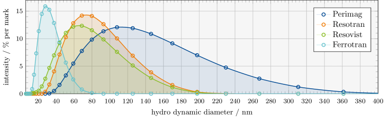
Figure 1: Intensity weighted log normal size distribution by DLS. A sample with a 1:100 dilution of each tracer was measured using DLS to determine the hydrodynamic particle diameter, that includes the dextran shell coating (laser wavelength of $633\text{\,}$, $30\text{\,}$ measurement time, $3$ averages).

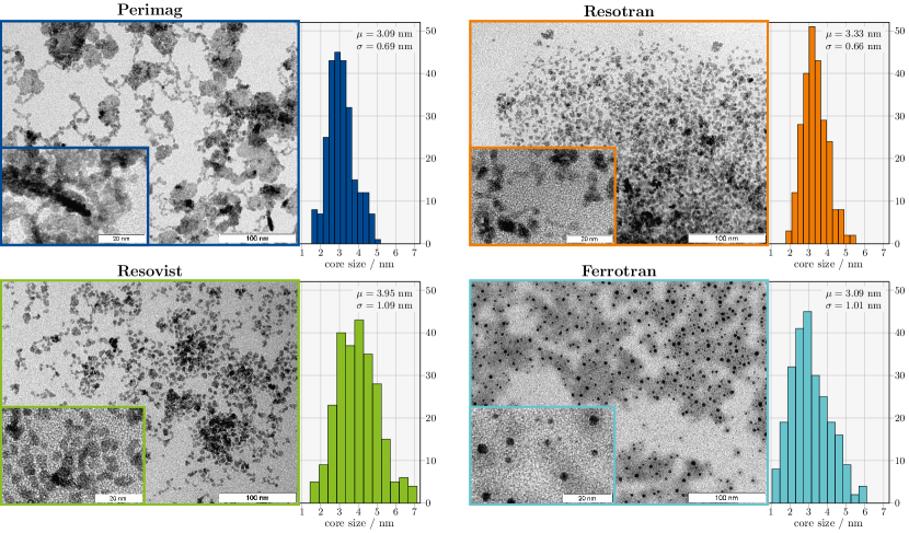
Figure 2: TEM images. Samples of each tracer as visualized by TEM for two different zoom levels at $20\text{\,}$ and $100\text{\,}$ reference scale, showing the iron-oxide core. Each histogram lists the mean $\mu$ and the standard deviation $\sigma$ of the core short-axis diameter for a count of $n=250$ particles categorized into $12$ individual size bins. Note, that Perimag, Resotran and Resovist form clusters and chains, which were not counted, whereas Ferrotran accounts for the smallest and individual particles (USPIO).

Results of the DLS measurements are shown in figure 1. Light intensity is given in percent for each size bin (round marks) with respect to all measured bins of the log normal size distribution. Perimag exhibits the largest hydrodynamic sizes with a peak value at $114\text{\,}$ (z-average $102.5\text{\,}$, PDI 0.1853), followed by Resotran with a narrower distribution and a peak at $74\text{\,}$ (z-average $66.32\text{\,}$, PDI 0.1806). Resovist is roughly comparable to Resotran, with a peak value at $65\text{\,}$ (z-average $55.97\text{\,}$, PDI 0.2007). Ferrotran is a USPIO and has a hydrodynamic diameter of around $28\text{\,}$ (z-average $27.82\text{\,}$, PDI 0.09) and the narrowest distribution of all tracers.

3.2 Transmission Emission Microscopy

In figure 2, TEM images and a histogram of individual particles for a count of $n=250$ short-axis core diameter measurements are shown for each tracer. The mean $\mu$ and the standard deviation $\sigma$ are given in the top right corners. TEM images provide indications of shape, structure, size and uniformity of the nanoparticles. Note that the counting rule applied significantly influences the classification [bresch_counting_2022], but we mostly observe spherical individual particles without strong elongation and do not classify particle clusters.

Perimag and Ferrotran exhibit the smallest mean core diameter, followed by Resotran and Resovist in increasing order. As TEM images show the magnetite cores, clusters and particle-chains are visible as well as overlapping particles. Especially for Perimag, such clusters and chains are visible in the pictures and the cores tend to form large clusters in the range of $2050\text{\,}$. Visual inspection of Resotran and Resovist indicates a similar structure and size of both tracers. Ferrotran shows isolated cores, separated by their ligand hull, which reduces magnetic interaction in between particles. Seemingly, no clusters are formed and particles do not overlap, which agrees with DLS results for this USPIO.

3.3 Vibrating Sample Magnetometer

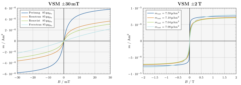
Figure 3: VSM results. The magnetic moment is plotted against the external field for two different ranges with identical samples. The steeper the slope of the net magnetic moment $m$ at the origin, the stronger is the nonlinear response which is the useful signal in MPI.

The results of the VSM measurements are shown in figure 3. All particle samples show the expected superparamagnetic behavior with sigmoidal magnetization curves and no detectable hysteresis. In the $\pm$2\text{\,}$$ range plot, the magnetization curves of Resovist and Resotran are very similar, reaching almost the same saturation magnetization at about $83.6\text{\,}\mathrm{A}\mathrm{m}^{2}\mathrm{/}\mathrm{k}\mathrm{g}_{Fe}$. The saturation magnetization of Perimag is around $89.3\text{\,}\mathrm{A}\mathrm{m}^{2}\mathrm{/}\mathrm{k}\mathrm{g}_{Fe}$. Ferrotran has the highest saturation magnetization of the investigated particles ($93.88\text{\,}\mathrm{A}\mathrm{m}^{2}\mathrm{/}\mathrm{k}\mathrm{g}_{Fe}$), but has a much lower initial slope with an almost linear curve in the MPI relevant range $\pm$30\text{\,}$$, when the origin of the left plot in figure 3 is considered. In contrast, Perimag shows the strongest nonlinearity with an initial slope around $1.23\text{\,}\mathrm{\SIUnitSymbolMicro}\mathrm{A}\mathrm{m}^{2}\mathrm{/}\mathrm{m}\mathrm{T}$, whereas Resotran exhibits $0.67\text{\,}\mathrm{\SIUnitSymbolMicro}\mathrm{A}\mathrm{m}^{2}\mathrm{/}\mathrm{m}\mathrm{T}$ and Resovist is lower with $0.45\text{\,}\mathrm{\SIUnitSymbolMicro}\mathrm{A}\mathrm{m}^{2}\mathrm{/}\mathrm{m}\mathrm{T}$ (evaluated at $\pm$1\text{\,}$$).

3.4 Magnetic Particle Spectroscopy

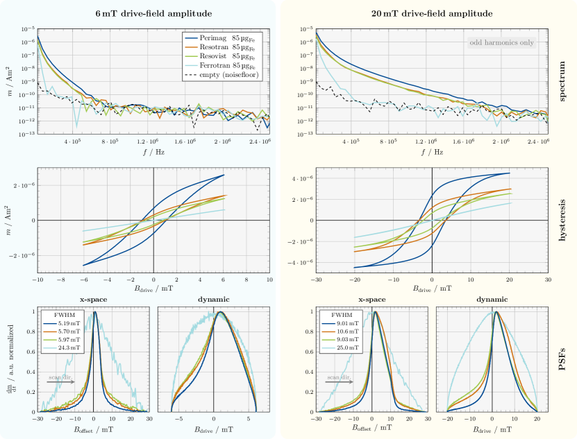
Figure 4: Arbitrary waveform MPS results. Spectrum, hysteresis and PSFs from top to bottom for $6\text{\,}$ and $20\text{\,}$ sinusoidal drive-field excitation. The frequency spectrum only contains odd harmonics of the fundamental $f_{1}=$26.042\text{\,}$$. The FWHM of the $x$-space PSF is given in the legend and the gray arrow indicates the scan direction (positive half-wave).

Four types of plots are generated in figure 4, each containing measurements of the four MNPs under investigation. On the top, the spectrum for $6\text{\,}$ and $20\text{\,}$ excitation amplitude is shown, because these amplitudes refer to a realistic range for human-sized MPI [ozaslan_pns_2022, thieben_system_2023]. We only plotted the odd harmonics, because they contain the majority of the information on the nonlinear magnetization of MNPs in a homogeneous sinusoidal excitation field (without offset fields). The spectrum of Resotran and Resovist are very similar for both $6\text{\,}$ and $20\text{\,}$, the amplitude of Resotran being slightly higher in the range of $515\text{\,}$. Compared to Resotran, Perimag has a $1.5$ to $2.0$-fold higher signal amplitude at low harmonic indices, increasing to $2.5$ at higher indices above $400\text{\,}$. Ferrotran has an overall low signal amplitude, as already indicated by the linear slope in figure 3. Even at $20\text{\,}$ excitation, useful signal is only detectable below $300\text{\,}$, indicating insufficient MPI signal.

In the middle row, the hysteresis curve is plotted, which shows a residual magnetization for all tracers, except for Ferrotran, which does not seem to undergo a measurable, relaxation-induced hysteresis. On the bottom the different normalized PSFs are plotted. We state the FWHM for the $x$-space PSF to facilitate comparison. At $6\text{\,}$, all tracers except Ferrotran indicate very similar magnetic properties, however, the difference in terms of FWHM between both PSF types are large. This effect reduces at $20\text{\,}$ with a trend for the $x$-space PSF to broaden and the dynamic PSF to narrow. Both PSFs indicate an inferior MPI image quality for Ferrotran. The noisy shape is caused by the normalization, which maps all peak amplitudes to one. Their original relation of maximum signal can be deduced from the saturation region of the hysteresis curve above.

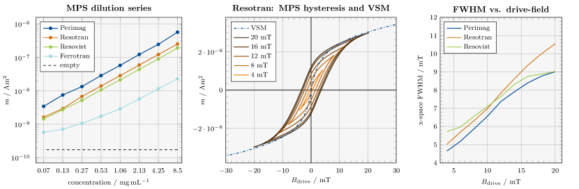
Figure 5: MPS data analysis. On the left, a dilution series of all tracers is shown. The absolute value of the third harmonic of exponentially decreasing concentrations between $8.5\cdot\left(\nicefrac{{1}}{{2}}\right)^{0}$  and $8.5\cdot\left(\nicefrac{{1}}{{2}}\right)^{7}$  is plotted ($20\text{\,}$, $26.042\text{\,}$). The center plot focuses on Resotran: the hysteresis for 5 different excitation amplitudes is plotted (bright to dark for increasing amplitude) with an overlay of the VSM curve (dash-dot). On the right, the FWHM is plotted against the drive-field amplitude. Ferrotran was omitted to retain a detailed scale.

In a deeper MPS analysis, we refer to three different types of plots in figure 5. On the left side, the results of the MPS dilution series are shown. We observe a linear behavior in the absolute magnitude of the third harmonic over all concentrations down to $8.5\cdot\left(\nicefrac{{1}}{{2}}\right)^{7}\approx 0.066~{}$$$ for Perimag, Resotran and Resovist. While Perimag produces the highest signal, the results indicate that Resotran and Resovist are relatively comparable in signal strength, with Resotran’s signal being slightly higher. Ferrotran gives a much weaker MPS signal, starting with a linear result for higher concentrations, but loosing linearity by the 4th dilution step towards lower concentrations. At the lowest two concentrations, the response is barely higher than the background signal.

In the center of figure 5, the hysteresis curve for Resotran is plotted in a range of