Fairness of Exposure in Online Restless Multi-armed Bandits

Abstract.

Restless multi-armed bandits (RMABs) generalize the multi-armed bandits where each arm exhibits Markovian behavior and transitions according to their transition dynamics. Solutions to RMAB exist for both offline and online cases. However, they do not consider the distribution of pulls among the arms. Studies have shown that optimal policies lead to unfairness, where some arms are not exposed enough. Existing works in fairness in RMABs focus heavily on the offline case, which diminishes their application in real-world scenarios where the environment is largely unknown. In the online scenario, we propose the first fair RMAB framework, where each arm receives pulls in proportion to its merit. We define the merit of an arm as a function of its stationary reward distribution. We prove that our algorithm achieves sublinear fairness regret in the single pull case $O(\sqrt{T\ln T})$, with $T$ being the total number of episodes. Empirically, we show that our algorithm performs well in the multi-pull scenario as well.

1. Introduction

Bandit algorithms have gained increasing popularity in recent years in modelling decision-making problems where the decision-maker interacts with an unknown environment. At each round, the decision maker has to choose a subset of choices or arms, resulting in certain rewards for the decision maker. The goal, therefore, is to focus both on learning the environment while also choosing arms in such a way as to maximize the total reward. Bandit algorithms are useful in various applications ranging from marketing Rothschild (1974), crowdsourcing  Abraham et al. (2013), resource allocations Berry and Fristedt (1985), healthcare Biswas et al. (2021); Killian et al. (2023a), etc.

Restless Multi-Armed Bandits (RMABs) are a class of MABs where each arm has a Markov Decision Process (MDP) associated with it. Each arm has its own states, actions, transition dynamics, and reward functions. In RMABs, the number of actions associated with each arm could be two or more two Hodge and Glazebrook (2015); Killian et al. (2021b, a). In line with most of the literature, we consider two actions per arm – to pull or not pull the arm  Whittle (1988); Jung and Tewari (2019); Biswas et al. (2021); Wang et al. (2023). A slightly different line of work is around rested bandits, where at each round, only the arms that receive a pull transition from one state to another. However in restless bandits, all the arms transition from one state to the next state, irrespective of whether they are pulled or not. In RMABs, since arms transition irrespective of whether pulled or not, they exhibit different transition dynamics for the action taken (pull/not pull). It is this restless nature of the arms that makes RMABs applicable to many domains such as network scheduling  Modi et al. (2019), anti-poaching  Qian et al. (2016), healthcare  Mate et al. (2022), etc.

Recently, a lot of works have been using restless bandits to model preventive interventions in public healthcare scenarios  Biswas et al. (2021); Herlihy et al. (2023); Killian et al. (2023a); Mate et al. (2020); Killian et al. (2023b). Here, each arm corresponds to a patient or a beneficiary, whereas the decision maker may be a public hospital or agency that provides intervention to these patients. Providing an intervention to each patient is considered equivalent to pulling an arm. Because of the limited resources, such as the limited number of workers working at the hospital or agency, intervention can be provided to only a limited number of patients at a time. When intervened, each patient’s state (good/bad) changes depending on whether they received the intervention or not. It is essential to look for policies that provide the maximum benefit to the public, i.e., policies that ensure most patients remain in a good state for longer.

Some of the preliminary literature on restless bandits assumes that the transition dynamics for each arm’s MDP are known i.e. offline setting. In general, it has been proven that finding an optimal policy for RMABs even when the transition dynamics are known is PSPACE-hard  Papadimitriou and Tsitsiklis (1994).  Whittle (1988) provided an indexing policy that is asymptotically optimal given that the arms are indexable  Weber and Weiss (1990); Akbarzadeh and Mahajan (2019). Recently, there have been some advancements in online setting, where these transition dynamics are not known and are learned over a period of time. To this, researchers have explored Thompson Sampling Jung and Tewari (2019); Jung et al. (2019), Upper Confidence Bound (UCB) Ortner et al. (2012); Wang et al. (2023) and Model-free Q-learning approaches  Fu et al. (2019); Avrachenkov and Borkar (2022); Biswas et al. (2021), among many others. However, all these approaches focus only on finding the optimal policy – leading to some arms being completely ignored Prins et al. (2020). As in our running example where arms model patients, this represents a major problem: the optimal policies would focus only on patients who require the most interventions and ignore the patients who rarely need interventions. However, in public healthcare, it becomes important to focus on all kinds of patients and not just a few, so as to provide unbiased healthcare to society.

Fairness in RMABs is an upcoming research direction that seeks to address this problem. Current work on fairness in RMABs primarily focuses on the offline setting Herlihy et al. (2023); Li and Varakantham (2023); Prins et al. (2020); Mate et al. (2021). Only a few fairness notions are prevalent in the literature on the restless bandits setting. The first notion ensures that each arm should be pulled at least once every fixed time period Li and Varakantham (2022), and the second notion provides a lower bound on each arm’s probability of receiving a pull by user-defined constants Herlihy et al. (2023). These two fairness notions do not consider the heterogeneity of arms and introduce universal fairness constraints.  Li and Varakantham (2023) talk about allocation vectors and that a more rewarding allocation vector should be chosen with a higher probability than a worse allocation vector. It still does not guarantee a minimum exposure guarantee to each arm and in worst case scenario can lead to some arms barely receiving pulls. Thus, it is a much weaker fairness notion.  Killian et al. (2023a) considers equitable group fairness where each arm belongs to a particular group, and the fairness notion provides enough exposure to each group so as to ensure equal outcomes. In this approach as well, the pulls may be still distributed unfairly within a group. Moreover, it requires apriori knowledge of which group an arm belongs to. Further, all the above works assume that the transition dynamics are known beforehand and construct their policies based on this assumption. To our knowledge, only Li and Varakantham (2022) explore fairness in online RMABs, where they consider equality focused fairness with universal fairness constraints. Therefore, there is a need to design online RMABs with stronger fairness guarantees.

We propose that fairness should be defined with respect to the steady-state distribution of the MDPs of the arms. The steady-state is important because it talks about the state that the arms would end up in when we run a policy sufficiently long, which would happen in a real-world setting. We define the goodness of an arm by the difference in the steady-state distribution of the arm being in the good state when we always pull the arm, compared to when we never pull the arm. This metric is indicative of how much an arm benefits from intervention. If we did not use the difference and instead just chose the steady state probability of being in the good state to be the merit of an arm, then it may so happen that this arm would have ended up in the good state without even needing intervention, and we would have wasted our limited budget on an arm which did not necessarily need it. Taking the difference helps us identify the arms that are impacted the most by our help. Once we have a notion of the merit of an arm, one can define meritocratic fairness similar to that of Wang et al. (2021). We call our notion of fairness as Merit Fair  where each arm is pulled with probability proportional to how much benefit we obtain at a steady state by pulling the arm. Merit Fair notion is better than the existing notions in RMABs because it does not use any universal fairness constant like in Li and Varakantham (2022); Herlihy et al. (2023), but rather provides exposure to each arm based on its merit.

Generally, a multiple pull setting is considered in RMABs which means that at each round, the public hospital makes a call to K patients to be intervened. In this paper, for theoretical analysis, we primarily focus on single pull settings for the following reasons. Meritocratic fairness Wang et al. (2021) has been specially designed for pulling a single arm at each round. It is not clear how such merit-based fairness can be extended beyond multiple pulls. We show that extending merit-based fairness to multiple pulls will require some technical assumptions, which may not necessarily hold in practice. Even if such technical requirements are satisfied, with multiple pull RMAB, quantifying fairness is challenging. For example, suppose we have a budget to pull all the arms, then we will not be able to learn transition probabilities of action ‘not pulling’ the arm effectively unless we forgo pulling an arm despite having the available budget. Hence, in this work, we focus on single-pull settings for theoretical aspects, though our algorithm can be extended to multiple pulls. Therefore, we study its efficacy on multiple pull settings on synthetic and real-world datasets. To the best of our knowledge, we are the first one to provide theoretical results in the online fair RMAB problem, and also the first one to extend the Fairness of Exposure Wang et al. (2021) notion to Restless bandits. Our core contributions are:

• We extend the exposure fairness notion of  Wang et al. (2021) to an online RMAB setting.

• We provide a sublinear bound on fairness regret when only one arm is pulled and provide experimental results on both single pull and multiple pull cases.

• We validate the efficacy of our proposed algorithm on synthetic and real-world datasets  Kang et al. (2016).

The paper is structured as follows. Section 2 summarizes the required literature background. In Section 3, we define preliminaries and notations used consistently throughout the paper. Section 4 provides details to our approach and Section 5 provides its theoretical guarantees. We validate the efficacy of our method on real and synthetic data in Section 6.

2. Related Work

2.1. Restless Bandits

Whittle  Whittle (1988) provides an asymptotically optimal indexing approach for RMABs when the transition dynamics are known. When the transition dynamics are unknown, previous works include Thompson Sampling based approaches  Jung and Tewari (2019); Jung et al. (2019) which construct policies based on a prior and then update the prior according to the feedback from the environment; Upper Confidence Bound based approaches  Ortner et al. (2012); Wang et al. (2023) which maintain a confidence region for the transition dynamics and construct policies based on this region; and model-free approaches  Fu et al. (2019); Avrachenkov and Borkar (2022); Biswas et al. (2021) which skip learning the environment dynamics altogether and only focus on finding the Whittle indices to determine the optimal action to take in each round. In this paper, we will be using upper confidence bound-based approaches to learn the transition dynamics.

2.2. Fairness in MAB

There have been multiple approaches to address fairness in multi-armed bandits. Here, we discuss some fairness notions available in the literature concerning stochastic bandits setting  Joseph et al. (2016); Heidari and Krause (2018); Li et al. (2019); Chen et al. (2020); Patil et al. (2021); Wang et al. (2021).  Joseph et al. (2016) use the idea that a better arm is always selected with greater or equal probability than a worse arm. This fairness notion, while good for the optimal arm, may lead to many arms getting very minimal exposure. Later, some works define fairness in terms of providing minimum/maximum amount of exposure to each of the arms  Heidari and Krause (2018); Li et al. (2019); Chen et al. (2020). On similar lines,  Patil et al. (2021) achieve anytime fairness guarantee, i.e., at each round, every arm will be pulled at least a fixed predetermined fraction of times. This notion requires the user to input a predetermined vector quantifying the exposure required for each arm. Later,  Wang et al. (2021) extended the fairness notion to proportional fairness which requires that each arm be pulled with a probability proportional to its merit. The authors compare their algorithm with an optimal fair benchmark, which is aware of the true merit of each arm and does not need to learn anything.

2.3. Fairness in RMAB

Fairness in Restless Bandits has only recently started to be explored. Offline algorithms, which assume full knowledge of the transition dynamics of each arm, include  Herlihy et al. (2023) which ensures that the probability of each arm being pulled is in the interval $[l,u]$ where $l,u$ are user-defined parameters.  Li and Varakantham (2023) provide the fairness notion that an allocation vector should always be chosen with greater or more probability than a worse allocation vector.  Prins et al. (2020) consider RMABs where only the states of the arms that are pulled are observable and the rest are not, and their fairness notion is that each arm should be pulled at least once every fixed period of time.  Mate et al. (2021) show that their reward function can be shaped so as to incentivize fairness. Finally,  Killian et al. (2023a) consider group fairness and frames the problem so as to find the allocation among the groups that maximizes the total social welfare. In an online setting,  Li and Varakantham (2022) provide a Q-learning Whittle Indexed based algorithm that operates similarly to  Patil et al. (2021); Chen et al. (2020). Their fairness constraint that each arm receives a pull every fixed time period does not take into account the heterogeneity of the arms and they do not discuss any notions of regret while learning. Our work combines the fairness notion of  Wang et al. (2021), the Online RMAB approach of  Wang et al. (2023), and the steady state reward formulation of  Herlihy et al. (2023), to provide a novel analysis on regret in online Fair RMABs.

3. Preliminaries

An RMAB problem is defined by a set of $N$ independent arms. Each arm $i\in[N]$ is characterized by a Markov Decision Process (MDP) given by $(\mathcal{S},\mathcal{A},\mathcal{R},P_{i})$ with $\mathcal{S},\mathcal{A}$, and $\mathcal{R}:\mathcal{S}\xrightarrow{}\mathbb{R}$ denoting the state space, action space, and reward function respectively. $P_{i}:\mathcal{S}\times\mathcal{A}\times\mathcal{S}\xrightarrow[]{}[0,1]$ is the transition probablity matrix for arm $i$. In the traditional RMAB setting, $\mathcal{S},\mathcal{A},\mathcal{R}$ are taken to be common among all the arms, and each arm differs only by their transition matrix $P_{i}$. The states are assumed to be fully observable. The action the decision-maker takes is governed by a policy $\pi$. The total number of episodes is $T$, where a policy $\pi^{t}$ is fixed for $t\leq T$, and is run for $H$ timesteps, where $H$ is the time horizon of an episode. For each timestep $h\in H$ in episode $t$, the decision-maker has to select $K\leq N$ arms according to $\pi^{t}$, where $K$ is the budget.

In our setting, we assume $\mathcal{S}\coloneqq\{0,1\}$, where 0 denotes bad state and 1 denotes good state. There are two possible actions, i.e. $\mathcal{A}\coloneqq\{1,0\}$, indicating whether an arm is pulled or not respectively. We take the reward as $\mathcal{R}(s)=s\ \forall s\in\mathcal{S}$, i.e., we receive a reward of 1 when the arm is in the good state and a reward of 0 when the arm is in the bad state. As the state and action spaces are discrete and finite, we can view the transition matrix $P_{i}$ as a $|\mathcal{S}|\times|\mathcal{A}|\times|\mathcal{S}|$ dimensional matrix where $P_{i}(s,a,s^{\prime})\in[0,1]$ is the probability of transitioning to state $s^{\prime}$ if action $a$ is taken while in state $s$.

In an online setting, $P_{i}$’s are unknown and need to be learned over multiple episodes. Let us denote the true transition matrix for an arm $i$ as $P^{*}_{i}$. We assume that $P^{*}_{i}$’s are non-degenerate, i.e., there exists an $\epsilon>0$ such that $\epsilon\leq P_{i}^{*}(s,a,s^{\prime})\leq 1-\epsilon\ \ \ \forall i\in[N],a\in\mathcal{A},s,s\in\mathcal{S}^{\prime}$. Intuitively, this means there is no deterministic transition, and there is always a non-zero chance of ending up in any state after action. This is a natural assumption and maps many real-life scenarios such as healthcare applications where there are rarely any deterministic transitions.

3.1. Merit Fair: Merit-based fairness in RMAB

To define meritocratic fairness for the arms, we must define a certain merit of pulling to each arm. As standard in the MAB literature, we refer to it also as a reward. Let $\mu_{i}^{*}$ denote the true reward of arm $i$, which we define formally later. Along a similar line to Wang et al.  Wang et al. (2021), let us define the Optimal Fair Policy as $Pr^{*}(K)$, where $Pr^{*}_{i}(K)$ is the probability that arm $i$ is among the $K$ chosen out of the $N$ total arms. Observe that $Pr^{*}_{i}(N)$ = 1 and that $Pr^{*}_{i}(1)$ = $\pi_{i}^{*}$, where $\pi^{*}$ is the probability distribution of being chosen over the arms. Note that $\sum_{i}\pi_{i}^{*}=1$ irrespective of $K$. Let $g(\cdot)$ be a non-decreasing merit function that maps the reward of the arm to a positive value. Then, for the optimal fair policy, the following equation holds.

$$\frac{Pr_{i}^{*}(K)}{g(\mu_{i}^{*})}=\frac{Pr_{j}^{*}(K)}{g(\mu_{j}^{*})}\ \ \forall i,j\in[N]$$ (1)

This implies that the exposure each arm gets is proportional to its merit. However, observe that if there is an arm $l$ such that $g(\mu_{l})>K\times g(\mu_{i})\;\forall i\neq l$, the probability of pulling the arm $l$ becomes more than $1$ to ensure desired fairness. Thus, we cannot guarantee such meritocratic fairness for multiple pulls. Even if we assume $g(\cdot),\ \mu^{\prime}s$ are such that $Pr_{i}(\cdot)<1\;\forall i$, there are further challenges in learning $P_{i}$’s for large $K$. Hence, for theoretical analysis, we focus on $K=1$. Note that for $K=1$, Equation (1) becomes

$$\frac{\pi_{i}^{*}}{g(\mu_{i}^{*})}=\frac{\pi_{j}^{*}}{g(\mu_{j}^{*})}\ \ \forall i,j\in[N]$$ (2)

Let $\pi=\{\pi^{t}\}_{t=1}^{T}$ be the policy learnt by our algorithm with $\pi^{t}$ being the employed policy at episode $t$. We define Fairness Regret $FR^{T}$ as the difference between the optimal fair policy $\pi^{*}$ and our policy $\pi$ up to episode $T$. Mathematically,

$$FR^{T}=\sum_{t=1}^{T}\sum_{i\in[N]}\left|\pi_{i}^{*}-\pi_{i}^{t}\right|$$ (3)

Here, $\pi_{i}^{t}$ denotes the probability of pulling an arm $i$ in episode $t$. We note that the notion of Reward Regret is also defined in  Wang et al. (2021) which we do not analyze it in this work. This is because Wang et al. (2021) discusses the stochastic MAB setting, where the reward of the arm is the actual reward we get after pulling the arm. In our case, we define $\mu_{i}^{*}$ in such a way that it only represents the benefit of pulling an arm, and only exists to indicate which arm is better suited for receiving a pull. It does not correlate to the actual reward (given by the reward function $\mathcal{R}$) that we receive after pulling some arm. Therefore, the concept of reward regret does not make much sense in our work. For the sake of the theoretical analysis of the regret, we impose the same conditions on the merit function $g(\cdot)$ as imposed in  Wang et al. (2021).

Condition 3.1.

Merit of each arm is positive, i.e., $\min_{\mu}g(\mu)\geq\gamma$ for some $\gamma$ ¿ 0.

Condition 3.2.

Merit function is L-Lipschitz continuous, i.e., $\forall\mu_{1},\mu_{2},\\ {|g(\mu_{1})-g(\mu_{2})|}\leq{L|\mu_{1}-\mu_{2}|}$ for some constant L ¿ 0.

4. Methodology

4.1. Defining the reward

We first define a reward that is based on steady state and is indicative of how much intervention an arm requires. Consider the policy discussed by  Herlihy et al. (2023) where each arm is pulled with some fixed probability $p_{i}$. Then this policy can be defined as $\pi_{PF}:\{i\ |\ i\in[N]\}\xrightarrow{}[1-p_{i},\ p_{i}]^{N}$. Repeated application of this policy will result in a steady state distribution that tells us the probability of an arm being in state 1. Let us denote $f(P_{i},p_{i})$ to be the steady state probability of arm $i$ being in state 1, when followed a policy $\pi_{PF}$. Once, we acquire these probabilities, the reward of an arm can be naturally defined as:

$$\mu_{i}=f(P_{i},1)-f(P_{i},0)$$ (4)

This reward signifies the difference at steady state when we always pull arm $i$ as compared to when we never pull that arm. In other words, the reward represents the benefit of pulling an arm in the long run as compared to the loss the algorithm would have incurred if it had not pulled the arm.

We can now calculate the steady state probabilities as follows. If the transition matrix for arm $i$ is $P_{i}$, at steady state, we should have

$$f(P_{i},p_{i})[(1-p_{i})P_{i}(1,0,1)+p_{i}P_{i}(1,1,1)]\ +$$

$$(1-f(P_{i},p_{i}))[(1-p_{i})P_{i}(0,0,1)+p_{i}P_{i}(0,1,1)] =f(P_{i},p_{i})$$

After simplifying the above expression, we get, $f(P_{i},p_{i})=$

$$\frac{(1-p_{i})P_{i}(0,0,1)+p_{i}P_{i}(0,1,1)}{1-(1-p_{i})P_{i}(1,0,1)-p_{i}P_{i}(1,1,1)+(1-p_{i})P_{i}(0,0,1)+p_{i}P_{i}(0,1,1)}$$ (5)

We can then simplify reward $\mu_{i}$ as:

$$\mu_{i}=\frac{P_{i}(0,1,1)}{1-P_{i}(1,1,1)+P_{i}(0,1,1)}-\frac{P_{i}(0,0,1)}{1-P_{i}(1,0,1)+P_{i}(0,0,1)}$$

After defining the reward of the arms, we can continue towards the fairness notions discussed in Section  3.1. If we were to pull a single arm in every round, then Wang et al. (2021) proved that a unique fair policy satisfying Equation (1) is given by: $\pi^{*}_{i}=\frac{g(\mu_{i})}{\sum_{j\in N}g(\mu_{j})}$.

We will explain the process of pulling multiple arms later. It is further to be noted that the reward of an arm $i$ only depends on the probability transition matrix $P_{i}$ which is not known beforehand. The next subsection describes the procedure to learn these probability transition matrices using upper confidence bound techniques.

4.2. Online RMAB

As we are in an online setting, we seek to estimate the true transition matrices $P_{i}^{*}$’s. We use the Upper Confidence Bound (UCB) approach which maintains an optimistic bound on the true transition matrix corresponding to each state-action-state  Wang et al. (2023). The estimated value of the transition probability matrix of an arm for each $(s,a,s^{\prime})$ can be computed by finding a fraction of the time in which the arm transitioned to state $s^{\prime}$ from state $s$, when action $a$ was taken. This estimate and the number of times the arm was in state $s$ and action $a$ is considered, and a confidence radius is then created. It could further be proved that with high probability, the true transition matrix would lie within the confidence radius of the estimated transition matrix. We explain the detailed procedure below.

Let $N_{i}^{t}(s,a,s^{\prime})$ be the number of times $(s,a,s^{\prime})$ transition has been observed for arm $i$ by episode $t$. Further, define $N_{i}^{t}(s,a)=\sum_{s^{\prime}}N_{i}^{t}(s,a,s^{\prime})$ to be the total number of times arm $i$ had been in state $s$ when action $a$ is taken. Then at episode $t$, we estimate the true transition matrix $P_{i}^{*}(s,a,s^{\prime})$ with empirical mean

$$\hat{P}_{i}^{t}(s,a,s^{\prime})\coloneqq\frac{N_{i}^{t}(s,a,s^{\prime})}{N_{i}^{t}(s,a)}$$

and confidence radius

$$d_{i}^{t}(s,a)\coloneqq\sqrt{\frac{2|\mathcal{S}|\ln(2|\mathcal{S}||\mathcal{A}|N\frac{t^{4}}{\delta})}{\max\{1,N^{t}_{i}(s,a)\}}}$$ (6)

where $\delta>0$ is a user defined constant. We can now define the ball $B^{t}$ of possible values of $P^{*}$ as

$$B^{t}=\{P\ |\ \|{P}_{i}(s,a,\cdot)-\hat{P}_{i}^{t}(s,a,\cdot)\|_{1}\leq d_{i}^{t}(s,a)\ \forall i,s,a\}$$ (7)

In particular, $B_{i}^{t}$ is the ball of possible values of $P_{i}^{*}$ at episode $t$ for some particular arm $i$. It is not difficult to prove that with high probability, $P_{i}^{*}$ will lie in the ball $B_{i}^{t}$ (see Proposition 5.3 in Section 5). Therefore, throughout the paper, whenever we refer to valid transition matrices, it implies that the transition matrices lie in $B^{t}$. As there are only two states, the confidence region can be simplified further. $\forall P\in B^{t}$, we have that for $\forall i,s,a$,

$$\|{P}_{i}(s,a,\cdot)-\hat{P}_{i}^{t}(s,a,\cdot)\|_{1}\leq d_{i}^{t}(s,a)$$

$$\implies|{P}_{i}(s,a,1)-\hat{P}_{i}^{t}(s,a,1)|+|{P}_{i}(s,a,0)-\hat{P}_{i}^{t}(s,a,0)|\leq d_{i}^{t}(s,a)$$

$$\implies|{P}_{i}(s,a,1)-\hat{P}_{i}^{t}(s,a,1)|+|(1-{P}_{i}(s,a,1))-(1-\hat{P}_{i}^{t}(s,a,1))|\leq d_{i}^{t}(s,a)$$

$$\implies|{P}_{i}(s,a,1)-\hat{P}_{i}^{t}(s,a,1)|\leq\frac{d_{i}^{t}(s,a)}{2}$$

Similarly, $|{P}_{i}(s,a,0)-\hat{P}_{i}^{t}(s,a,0)|\leq\frac{d_{i}^{t}(s,a)}{2}$. Let us further define:

$$P_{i}^{+,t}(s,a,1)=\min\left\{1,\hat{P}_{i}^{t}(s,a,1)+\frac{d_{i}^{t}(s,a)}{2}\right\}$$

$$P_{i}^{-,t}(s,a,1)=\max\left\{0,\hat{P}_{i}^{t}(s,a,1)-\frac{d_{i}^{t}(s,a)}{2}\right\}$$

$$P_{i}^{+,t}(s,a,0)=\max\left\{0,\hat{P}_{i}^{t}(s,a,0)-\frac{d_{i}^{t}(s,a)}{2}\right\}$$

$$P_{i}^{-,t}(s,a,0)=\min\left\{1,\hat{P}_{i}^{t}(s,a,0)+\frac{d_{i}^{t}(s,a)}{2}\right\}$$

as the upper confidence and lower confidence bounds on the transition matrices. Note that $P_{i}^{+,t}$ is representative of optimistic transitions, as we are overestimating the probability of ending up in a good state. Let us also define the following: $\omega_{1,i}^{t}=P_{i}^{-,t}(1,1,1)-P_{i}^{+,t}(0,1,1),\omega_{2,i}^{t}=P_{i}^{-,t}(1,0,1)-P_{i}^{+,t}(0,0,1)$, $\eta_{1,i}^{t}=P_{i}^{+,t}(1,1,1)-P_{i}^{-,t}(0,1,1),\eta_{2,i}^{t}=P_{i}^{+,t}(1,0,1)-P_{i}^{-,t}(0,0,1)$. Here, $\omega_{1,i}^{t}$ denotes the lower bound on the difference in transition probability matrices of arm $i$ when it is pulled and goes from state 1 to state 1 and from 0 to 1, respectively. $\omega_{2,i}^{t}$ denotes lower bound on difference in transition probability matrices when arm is not pulled. $\eta_{1,i}^{t},\eta_{2,i}^{t}$ represents upper bounds of the same quantities. We make the following assumption throughout our work.

Assumption 4.1.

$\exists t_{0}<T$ that for $\forall t>t_{0}$, $\eta_{1,i}^{t},\eta_{2,i}^{t}<1\ \forall i\in[N]$

Assumption  4.1 discusses the estimated gap in two different transition probabilities. Note that as we are talking about probabilities, that gap can be at most 1. Our assumption is that by $t_{0}$ episodes, the confidence radius $d_{i}^{t}(\cdot\ ,\cdot)$ shrinks enough to make the gap strictly less than 1. This is not a strong assumption, as more and more times the state-action pairs are visited, the confidence region keeps shrinking as the radius is inversely proportional to $N_{i}^{t}(s,a)$. We provide empirical values of $t_{0}$ in Table  1 in Section  6. Overall, from our simulations, we see that $t_{0}$ remains low (¡40).

4.3. MF-RMAB

We now define our algorithm MF-RMAB  as follows. For each episode $t$, calculate the estimated reward of each arm $i$ as $\mu_{i}^{t}=f(P_{i}^{+,t},1)-f(P_{i}^{+,t},0)$. Then the probability distribution over arms being chosen $\pi^{t}$ is given by

$$\pi_{i}^{t}=\frac{g(\mu_{i}^{t})}{\sum_{j}g(\mu_{j}^{t})}$$ (8)

It is very important to observe that we can also take any other $P_{i}^{t}\in B_{i}^{t}$ while estimating the reward (line 5 of Algorithm  1). As a matter of fact, our regret proofs hold for any set of valid transition matrices. MF-RMAB takes the upper bound on transition matrices as they are indicative of the upper bound of transitioning to the good state, and we wish to be optimistic about each arm’s capability of transitioning to the good state. If an arm is more likely to transition to the good state, then it would lead to the arm being in the good state with a higher probability in the steady state, which is what we wish to achieve. We then sample K arms from this probability distribution without replacement. When $K=1$, the probability of an arm $i$ being chosen is $Pr_{i}^{t}(K)=Pr_{i}^{t}(1)=\pi_{i}^{t}$, and when $K>1$, the probability of arm $i$ being chosen will be $Pr_{i}^{t}(K)\geq Pr_{i}^{t}(1)=\pi_{i}^{t}$. As the probability of being pulled is greater than that of our defined fair policy Equation (2), MF-RMAB is still fair based on the defined fairness. The complete pseudo code for MF-RMAB is given in Algorithm  1.

Data: No. of arms, budget K, time horizon H, no. of episodes T, merit function g($\cdot$)

1 $N_{i}^{t}(s,a,s^{\prime})\leftarrow 0\ \forall t,i,s,a,s^{\prime}$;

2 for $t=1$ to $T$ do

3       for $i=1$ to $N$ do

4             Estimate $\hat{P}_{i}^{t}(s,a,s^{\prime})$ and $d_{i}^{t}(s,a)$ using $N_{i}^{t}(s,a,s^{\prime})\ \forall s,a$;

5             $\mu_{i}^{t}\leftarrow f(P_{i}^{+,t},1)-f(P_{i}^{+,t},0)$;

6            

7       end for

8      $\pi^{t}\leftarrow\left(\pi_{i}^{t}\ \forall i\ |\pi_{i}^{t}=\frac{g(\mu_{i}^{t})}{\sum_{j}g(\mu_{j}^{t})}\right)$ ;

9       for $h=1$ to $H$ do

10             Sample K arms from $\pi^{t}$;

11             Pull the sampled K arms;

12             Observe transitions $(s,a,s^{\prime})$ for all arms;

13            

14       end for

15      Update counts $N_{i}^{t}(s,a,s^{\prime})\ \forall i,s,a,s^{\prime}$;

16      

17 end for

Algorithm 1 MF-RMAB

5. Theoretical Results

We now provide the bound for fairness regret of MF-RMAB. First, we show through the following lemma that if we take any set of valid transition matrices, define the corresponding reward, and then define the corresponding probability distribution $\pi^{t}$ (Equation  8), then for arm $i$, both the states (0 and 1) are visited and both the actions (pull and no pull) are taken in some interval $G_{i}$.

Lemma 5.1.

For arm $i$, take any $P_{i}^{t}\in B_{i}^{t}$, define $\mu_{i}^{t}=f(P_{i}^{t},1)-f(P_{i}^{t},0)$. Define a policy using Equation  (8). Then, $\exists G_{i}<T$ such that $N_{i}^{t+G_{i}}(s,a)-N_{i}^{t}(s,a)>0\ \forall s,a$. In other words, after every $G_{i}$ episodes, arm $i$ has all its state-action pairs $(s,a)$ visited at least once.

Proof.

Since $g(\cdot)$ is a non-decreasing merit function we have:

$\frac{g(-1)}{Ng(1)}\leq\pi_{i}^{t}\leq Pr_{i}^{t}(K)=\lambda<1$ unless $K=N$. For $K=N$, the fairness regret Equation (3) will trivially be linear with respect to time. Now for an arm $i$, let $A_{i}$ be the event that only one single state is visited in episode $t$ (of length H) and $B_{i}$ be the event that only one action is taken for the entire episode $t$. If the initial state of arm $i$ is $s_{0}$, then,

$$\mathbb{P}(A_{i}|s_{0}=0)=\prod_{h=1}^{H}\left((1-Pr_{i}^{t}(K))P_{i}^{*}(0,0,0)+Pr_{i}^{t}(K)P_{i}^{*}(0,1,0)\right)$$

$$\leq(1-\epsilon)^{H} \epsilon\leq P_{i}^{*}(s,a,s)\leq 1-\epsilon$$ ()

$$\mathbb{P}(A_{i}|s_{0}=1)=\prod_{h=1}^{H}\left((1-Pr_{i}^{t}(K))P_{i}^{*}(1,0,1)+Pr_{i}^{t}(K)P_{i}^{*}(1,1,1)\right)$$

$$\leq(1-\epsilon)^{H}$$

$$\mathbb{P}(A_{i})=\mathbb{P}(A_{i}|s_{0}=0)+\mathbb{P}(A_{i}|s_{0}=1)\leq 2(1-\epsilon)^{H}$$

$$\mathbb{P}(B_{i})=\prod_{h=1}^{H}Pr_{i}^{t}(K)+\prod_{h=1}^{H}(1-Pr_{i}^{t}(K))\leq\lambda^{H}+\left(1-\frac{g(-1)}{Ng(1)}\right)^{H}=B_{i}^{0}$$

Therefore, $\mathbb{P}(A_{i}\cup B_{i})\leq 2(1-\epsilon)^{H}+B_{i}^{0}-2B_{i}^{0}(1-\epsilon)^{H}$. Now, define $\psi^{H}_{i}$ as the probability that all state action pairs are visited in an episode, then

$$\psi_{i}^{H}=1-Prob(A_{i}\cup B_{i})\geq 1-\left(2(1-\epsilon)^{H}+B_{i}^{0}-2B_{i}^{0}(1-\epsilon)^{H}\right)$$

and thus we get an upper limit on $G_{i}=1/\psi_{i}^{H}$ ∎

Definition 5.2.

Define $G=\max_{i}\{G_{i}\},\eta=\max_{i,t>t_{0}}\{\eta_{1,i}^{t},\eta_{2,i}^{t}\},\\ \omega=\max_{i,t>t_{0}}\{\omega_{1,i}^{t},\omega_{2,i}^{t}\}$

Proposition 5.3.

Given $\delta>0$ and $t>1$, $Prob(P^{*}\in B^{t})\geq 1-\frac{\delta}{t^{4}}$

The proposition states that the set of true transition matrices $P^{*}$ lies in our confidence region $B^{t}$ with high probability. The proof follows directly from Proposition 6.1 of Wang et al. (2023). We in next theorem show that if we take any set of valid transition matrices and define the corresponding reward, then the difference between our estimated reward and true reward is upper bounded.

Theorem 5.4.

For all $t>t_{0}$, take any $P_{i}^{t}\in B_{i}^{t}$, define $\mu_{i}^{t}=f(P_{i}^{t},1)-f(P_{i}^{t},0)$ and $\mu_{i}^{*}=f(P_{i}^{*},1)-f(P_{i}^{*},0)$ according to Equation  (4). Then for $t>t_{0}$ and $\forall i\in[N]$,

$$|\mu_{i}^{t}-\mu^{*}_{i}|\leq\\ \frac{d_{i}^{t}(1,1)+2d_{i}^{t}(0,1)+d_{i}^{t}(1,0)+2d_{i}^{t}(0,0)}{(1-\eta)(1-\omega)}$$

Proof.

We have that for $t>t_{0}$, $\omega_{1,i}^{t}<P_{i}^{t}(1,1,1)-P_{i}^{t}(0,1,1)<\eta_{1,i}^{t}<1$ and $\omega_{2,i}^{t}<P_{i}^{t}(1,0,1)-P_{i}^{t}(0,0,1)<\eta_{2,i}^{t}<1$. So, we get

$$\frac{P_{i}^{t}(0,1,1)}{1-\omega_{1,i}^{t}}<f(P_{i}^{t},1)<\frac{P_{i}^{t}(0,1,1)}{1-\eta_{1,i}^{t}}$$

$$\frac{P_{i}^{t}(0,0,1)}{1-\omega_{2,i}^{t}}<f(P_{i}^{t},0)<\frac{P_{i}^{t}(0,0,1)}{1-\eta_{2,i}^{t}}$$

For some arm $i$ in episode $t$ with $t>t_{0}$, we drop notation $i,t$ by letting $f(1)=f(P_{i}^{t},1),f(0)=f(P_{i}^{t},0),f^{*}(1)=f(P_{i}^{*},1),f^{*}(0)=f(P_{i}^{*},0),\mu=f(P_{i}^{t},1)-f(P_{i}^{t},0),\mu^{*}=f(P_{i}^{*},1)-f(P_{i}^{*},0),\omega_{1,i}^{t}=\omega_{1},\omega_{2,i}^{t}=\omega_{2},\eta_{1,i}^{t}=\eta_{1},\eta_{2,i}^{t}=\eta_{2}$. Then

$$|\mu-\mu^{*}| =\lvert(f(1)-f(0))-(f^{*}(1)-f^{*}(0))\rvert$$

$$\leq|f(1)-f^{*}(1)|+|f(0)-f^{*}(0)|$$

$$\leq\left\lvert\frac{P(0,1,1)}{1-\eta_{1}}-\frac{P^{*}(0,1,1)}{1-\omega_{1}}\right\rvert+\left\lvert\frac{P(0,0,1)}{1-\eta_{2}}-\frac{P^{*}(0,0,1)}{1-\omega_{2}}\right\rvert$$

The first term $\left|\frac{P(0,1,1)}{1-\eta_{1}}-\frac{P^{*}(0,1,1)}{1-\omega_{1}}\right|$, can be bounded as

$$=\left|\frac{P(0,1,1)-P^{*}(0,1,1)-\omega_{1}P(0,1,1)+\eta_{1}P^{*}(0,1,1)}{(1-\eta_{1})(1-\omega_{1})}\right|$$

$$=\left|\frac{P(0,1,1)-P^{*}(0,1,1)-\omega_{1}(1-P(0,1,0))+\eta_{1}(1-P^{*}(0,1,0))}{(1-\eta_{1})(1-\omega_{1})}\right|$$

$$=\left|\frac{P(0,1,1)-P^{*}(0,1,1)+\omega_{1}P(0,1,0)-\eta_{1}P^{*}(0,1,0))+\eta_{1}-\omega_{1}}{(1-\eta_{1})(1-\omega_{1})}\right|$$

$$\leq\frac{|P(0,1,1)-P^{*}(0,1,1)|+|\omega_{1}P(0,1,0)-\eta_{1}P^{*}(0,1,0))+\eta_{1}-\omega_{1}|}{(1-\eta_{1})(1-\omega_{1})}$$

Now, $|\omega_{1}P(0,1,0)-\eta_{1}P^{*}(0,1,0))+\eta_{1}-\omega_{1}|$ can be bounded by

$$|\omega_{1}P(0,1,0)-\omega_{1}P^{*}(0,1,0)+\omega_{1}P^{*}(0,1,0)-\eta_{1}P^{*}(0,1,0))+\eta_{1}-\omega_{1}|$$

$$=|\omega_{1}(P(0,1,0)-P^{*}(0,1,0))-P^{*}(0,1,0)(\eta_{1}-\omega_{1})+\eta_{1}-\omega_{1}|$$

$$\leq|\omega_{1}(P(0,1,0)-P^{*}(0,1,0))+(\eta_{1}-\omega_{1})|$$

$$\leq|\omega_{1}||(P(0,1,0)-P^{*}(0,1,0)|+|\eta_{1}-\omega_{1}|$$

$$\leq|(P(0,1,0)-P^{*}(0,1,0)|+|\eta_{1}-\omega_{1}|$$

Also, $|\eta_{1}-\omega_{1}|=|(P^{+}(1,1,1)-P^{-}(0,1,1))-(P^{-}(1,1,1)-P^{+}(0,1,1))|\leq|P^{+}(1,1,1)-P^{-}(1,1,1)|+|P^{+}(0,1,1)-P^{-}(0,1,1)|=d(1,1)+d(0,1)$.

Therefore the first term, $\left|\frac{P(0,1,1)}{1-\eta_{1}}-\frac{P^{*}(0,1,1)}{1-\omega_{1}}\right|$, is bounded by:

$$\leq\frac{|P(0,1,1)-P^{*}(0,1,1)|+|(P(0,1,0)-P^{*}(0,1,0)|+d(1,1)+d(0,1)}{(1-\eta_{1})(1-\omega_{1})}$$

$$=\frac{\|P(0,1,\cdot)-P^{*}(0,1,\cdot)\|_{1}+d(1,1)+d(0,1)}{(1-\eta_{1})(1-\omega_{1})}$$

$$\leq\frac{d(0,1)+d(1,1)+d(0,1)}{(1-\eta_{1})(1-\omega_{1})}=\frac{d(1,1)+2d(0,1)}{(1-\eta_{1})(1-\omega_{1})}$$

We can similarly bound the second term. Going back to the original equation, we get

$$|\mu_{i}^{t}-\mu^{*}_{i}|\leq\frac{d_{i}^{t}(1,1)+2d_{i}^{t}(0,1)}{(1-\eta_{1,i}^{t})(1-\omega_{1,i}^{t})}+\frac{d_{i}^{t}(1,0)+2d_{i}^{t}(0,0)}{(1-\eta_{2,i}^{t})(1-\omega_{2,i}^{t})}$$

With $\eta=\max_{i,t>t_{0}}\{\eta_{1,i}^{t},\eta_{2,i}^{t}\}$, $\omega=\max_{i,t>t_{0}}\{\omega_{1,i}^{t},\omega_{2,i}^{t}\}$,

$$|\mu_{i}^{t}-\mu^{*}_{i}|\leq\frac{d_{i}^{t}(1,1)+2d_{i}^{t}(0,1)+d_{i}^{t}(1,0)+2d_{i}^{t}(0,0)}{(1-\eta)(1-\omega)}$$

∎

The next theorem states that if we take any set of valid transition matrices, define the corresponding reward, and then define the corresponding probability distribution $\pi^{t}$ (Equation  8), then our policy incurs a sublinear fairness regret when $K=1$.

Theorem 5.5.

Take any $P_{i}^{t}\in B_{i}^{t}$, define $\mu_{i}^{t}=f(P_{i}^{t},1)-f(P_{i}^{t},0)\\ \forall i\in[N]$. Define a policy using Equation  (8). Then for $T>t_{0}$, fairness regret of this policy when $K=1$ is $FR^{T}=\mathcal{O}\left(\frac{L\sqrt{GT\ln(8N\frac{T}{\delta})}}{\gamma(1-\eta)(1-\omega)}\right)$ with probability at least $1-\delta$.

Proof.

Fairness Regret $FR_{1}^{T}$ for $t>t_{0}$ when $P^{*}\in B^{t}$ can be bounded as:

$$fr^{t} =\sum_{i=1}^{N}|\pi_{i}^{t}-\pi_{i}^{*}|=\sum_{i=1}^{N}\left\lvert\frac{g(\mu_{i}^{t})}{\sum_{j=1}^{N}g(\mu_{j}^{t})}-\frac{g(\mu_{i}^{*})}{\sum_{j=1}^{N}g(\mu_{j}^{*})}\right\rvert$$

$$=\sum_{i=1}^{N}\left\lvert\frac{g(\mu_{i}^{t})\sum_{j=1}^{N}g(\mu_{j}^{*})-g(\mu_{i}^{*})\sum_{j=1}^{N}g(\mu_{j}^{t})}{\sum_{j=1}^{N}g(\mu_{j}^{t})\sum_{j=1}^{N}g(\mu_{j}^{*})}\right\rvert$$

$$\leq\frac{2\sum_{i=1}^{N}|g(\mu_{i}^{t})-g(\mu_{i}^{*})|}{\sum_{j=1}^{N}g(\mu_{j}^{t})} g(\mu_{i}^{*})\sum_{j=1}^{N}g(\mu_{j}^{*})$$ (Adding and subtracting in the numerator)

$$\leq 2\frac{\sum_{i=1}^{N}|g(\mu_{i}^{t})-g(\mu_{i}^{*})|}{N\gamma}\leq\frac{2L}{N\gamma}\sum_{i=1}^{N}|\mu_{i}^{t}-\mu_{i}^{*}|$$

$$\leq\frac{2L}{N\gamma}\sum_{i=1}^{N}\left(\frac{d_{i}^{t}(1,1)+2d_{i}^{t}(0,1)+d_{i}^{t}(1,0)+2d_{i}^{t}(0,0)}{(1-\eta)(1-\omega)}\right)$$

$$=\frac{2L}{N\gamma(1-\eta)(1-\omega)}\sum_{i=1}^{N}\left(d_{i}^{t}(1,1)+2d_{i}^{t}(0,1)+d_{i}^{t}(1,0)+2d_{i}^{t}(0,0)\right)$$

Next, we can bound $\frac{2L}{N\gamma(1-\eta)(1-\omega)}\sum_{i=1}^{N}d_{i}^{t}(s,a)$ as:

$$\frac{2L\sqrt{2|\mathcal{S}|\ln(2|\mathcal{S}||\mathcal{A}|N\frac{t^{4}}{\delta})}}{N\gamma(1-\eta)(1-\omega)}\sum_{i=1}^{N}\sqrt{1/\max\{1,N^{t}_{i}(s,a)\}}$$

$$\leq\frac{4L\sqrt{2|\mathcal{S}|\ln(2|\mathcal{S}||\mathcal{A}|N\frac{T}{\delta})}}{N\gamma(1-\eta)(1-\omega)}\sum_{i=1}^{N}\sqrt{1/\max\{1,N^{t}_{i}(s,a)\}}$$

Summing this term over time, we get:

$$\sum_{t=t_{0}+1}^{T}\frac{4L\sqrt{2|\mathcal{S}|\ln(2|\mathcal{S}||\mathcal{A}|N\frac{T}{\delta})}}{N\gamma(1-\eta)(1-\omega)}\sum_{i=1}^{N}\sqrt{1/\max\{1,N^{t}_{i}(s,a)\}}$$

$$=\frac{4L\sqrt{2|\mathcal{S}|\ln(2|\mathcal{S}||\mathcal{A}|N\frac{T}{\delta})}}{N\gamma(1-\eta)(1-\omega)}\sum_{i=1}^{N}\sum_{t=t_{0}+1}^{T}\sqrt{1/\max\{1,N^{t}_{i}(s,a)\}}$$

We defined $G_{i}$ as the expected number of episodes in the interval where all state-action pairs for arm $i$ is visited at least once. Then we have, $\sum_{t=t_{0}+1}^{T}\sqrt{1/\max\{1,N^{t}_{i}(s,a)\}}\leq\sum_{j=1}^{T/G_{i}}G_{i}/\sqrt{j}$. Note that $\sum_{j=1}^{T}1/\sqrt{j}\leq 2\sqrt{T}$. Therefore, $\frac{2L}{N\gamma(1-\eta)(1-\omega)}\sum_{t=t_{0}+1}^{T}\sum_{i=1}^{N}d_{i}^{t}(s,a)=\frac{2L\sqrt{2|\mathcal{S}|\ln(2|\mathcal{S}||\mathcal{A}|N\frac{t^{4}}{\delta})}}{N\gamma(1-\eta)(1-\omega)}\sum_{i=1}^{N}\sqrt{G_{i}T}$. With $G=\max_{i}G_{i}$, we get $FR_{1}^{T}=$

$$\sum_{t=1}^{T}\sum_{i\in[N]}\left|\pi_{i}^{*}-\pi_{i}^{t}\right|=\sum_{t=1}^{t_{0}}\sum_{i\in[N]}\left|\pi_{i}^{*}-\pi_{i}^{t}\right|+\sum_{t={t_{0}+1}}^{T}\sum_{i\in[N]}\left|\pi_{i}^{*}-\pi_{i}^{t}\right|$$

$$\leq Nt_{0}+\frac{48L\sqrt{2G|\mathcal{S}|T\ln(2|\mathcal{S}||\mathcal{A}|N\frac{T}{\delta})}}{\gamma(1-\eta)(1-\omega)}$$

As $|\mathcal{S}|=|\mathcal{A}|=2$, we get $FR_{1}^{T}\leq Nt_{0}+\frac{96L\sqrt{GT\ln(8N\frac{T}{\delta})}}{\gamma(1-\eta)(1-\omega)}$.

Note that Fairness Regret when $P^{*}\notin B^{t}$ is $FR_{2}^{T}\leq N\sqrt{T}$ with probability greater than $(1-\delta)$ ($\because Prob(P^{*}\in B^{t})\geq 1-\frac{\delta}{t^{4}}$).

Total Regret = $FR^{T}=FR_{1}^{T}+FR_{2}^{T}\leq Nt_{0}+N\sqrt{T}+\frac{96L\sqrt{GT\ln(8N\frac{T}{\delta})}}{\gamma(1-\eta)(1-\omega)}$ with probability greater than $1-\delta$ ∎

As MF-RMAB is defined using $P_{i}^{+,t}$, which is a valid transition matrix, we get the following corollary

Corollary 5.6.

For $t>t_{0}$, the fairness regret of MF-RMAB when $K=1$ is $FR^{T}=\mathcal{O}\left(\frac{L\sqrt{GT\ln(8N\frac{T}{\delta})}}{\gamma(1-\eta)(1-\omega)}\right)$ with probability at least $1-\delta$.

For $K>1$, the biggest challenge is to define an appropriate notion of fairness regret. One approach could be to take assumptions on $P^{*}$ and $g(\cdot)$ so that $\pi^{*}_{i}\leq\frac{1}{K};\forall i\in[N]$ which gives $\hat{FR}^{T}=\sum_{t=1}^{T}\sum_{i\in[N]}\left|\hat{\pi}_{i}^{*}-\hat{\pi}_{i}^{t}\right|$ where $\hat{\pi}_{i}=K\times\pi_{i}$. This new fairness regret $\hat{FR}^{T}$ would only differ by a factor of $K$ to $FR^{T}$ (Equation  3), and hence the sublinearity of Theorem  5.5 would still hold.

6. Experimental Section

We now validate the efficacy of MF-RMAB across different domains.

6.1. Domains

The three domains selected come from different values of true transition probabilities $P^{*}$.

Synthetic Dataset: Set the $P_{i}^{*}(s,a,s^{\prime})$ values uniformly in $[0,1]$ $\forall\ i\in[N],\ s,s^{\prime}\in\mathcal{S},\ a\in\mathcal{A}$

Synthetic-alternate Dataset: Similar to synthetic dataset, we set the $P_{i}^{*}(s,a,s^{\prime})$ values uniformly in $[0,1]$ $\forall\ i\in[N],\ s,s^{\prime}\in\mathcal{S},\ a\in\mathcal{A}$. In addition, the following two constraints are imposed on $P_{i}^{*}(s,a,s^{\prime})$. (1) Acting is always beneficial, i.e., $P_{i}^{*}(s,1,1)\geq P_{i}^{*}(s,0,1)\ \forall i\in[N]\ s\in\mathcal{S}$. (2) Starting in a good state is always beneficial, i.e., $P_{i}^{*}(1,a,1)\geq P_{i}^{*}(0,a,1)\ \forall i\in[N]\ a\in\mathcal{A}$.

CPAP Dataset: Continuous positive airway pressure therapy (CPAP) is considered to be a very effective treatment for obstructive sleep apnoea. However, some patients do not necessarily adhere to the therapy. We use the Markov model of CPAP treatment given by  Kang et al. (2016). We adapt their three-state model into two states in a similar fashion to  Herlihy et al. (2023); Li and Varakantham (2023). We combine states 2 and 3 into one state, and set the ratio of improvement of intervention $\alpha_{h}=1.1$. We set $30\%$ of the total arms as non-adherers (to the therapy). To add heterogeneity to the arms, we add Gaussian noise with mean $0$ and variance $0.1$ to each arm’s transition probabilities.

6.2. Experimental Setup

For the experimental evaluation of fairness regret, we compare MF-RMAB with an ”Optimal” baseline, where in each episode $t$, Optimal policy pulls the arms with the $K$ highest value for $\mu_{i}^{t}$. Observe that as $\mu_{i}\in[-1,1]$, we can trivially claim that in Conditions  3.1 and  3.2, $\gamma=g(-1)$ and $L=\max_{\mu_{1},\mu_{2}\in[-1,1]}\frac{g(\mu_{1})-g(\mu_{2})}{\mu_{1}-\mu_{2}}$ hold. We use $\delta=0.01$ and set the merit function $g(\mu)=e^{c\mu}$, implying that $\gamma=e^{-c}$ and $L=ce^{c}$. We set $c=3$ and provide additional experiments with different values of $c$ in the Appendix. In line with our non-degeneracy assumption on $P^{*}$, we clip the transition probabilities in the range $[\epsilon,1-\epsilon]$ with $\epsilon=0.01$ for all three datasets. We include an empirical comparison with FaWT-Q Li and Varakantham (2022) in the appendix. The results are averaged over 30 independent runs with different seed values.

We run the experiments for $T$=10k episodes and $H$=200 timesteps per episode for a total of $T\times H=2\times 10^{6}$ timesteps. We set the initial state of each arm randomly per episode. In accordance with our setting, we use a relatively high time horizon $H$, as our reward formulation and subsequent analysis are centered around steady state, and a longer time horizon would make it easier to achieve that steady state. For $K>1$ cases, we use the same definition of fairness regret (Equation  3) as for $K=1$ cases. The code is available at https://github.com/rchiso/MF-RMAB. The experiments were executed on a Xeon processor with 64 GB RAM.

6.3. Results

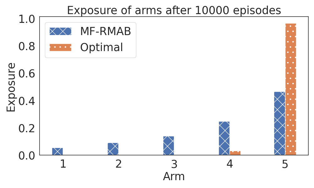
Figure 1. Exposure of arms under Optimal and MF-RMAB on Synthetic dataset after 10k episodes for $N=5$, $K=1$. The arms are arranged in increasing order of their rewards.

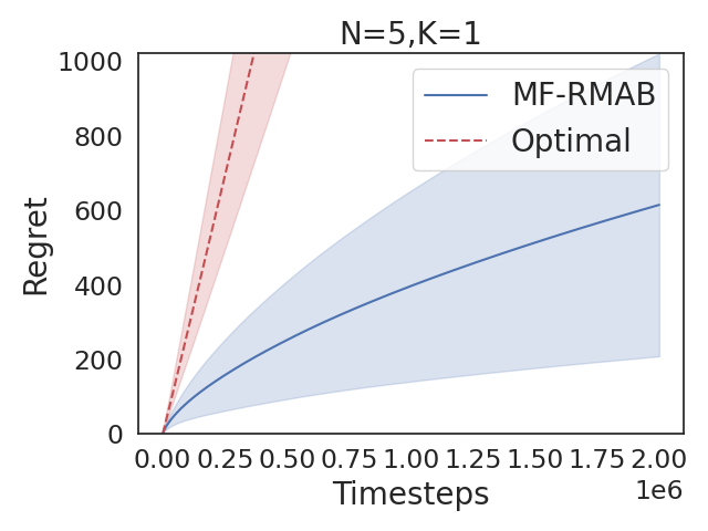
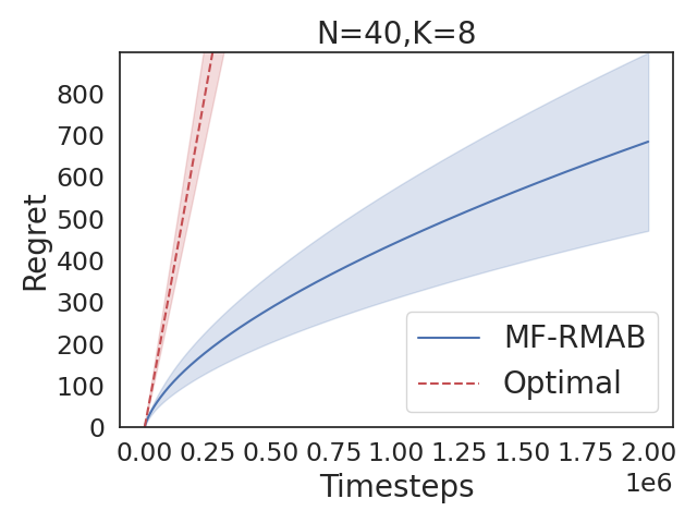
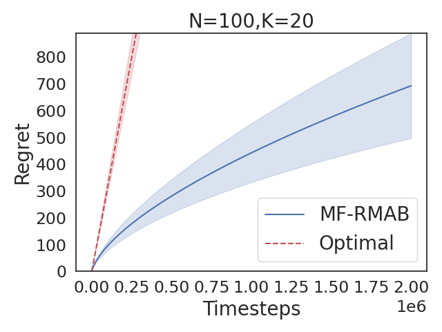
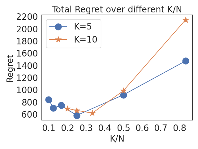
Figure 2. The first three plots show Regret vs. Time for different $K$ and $N$ settings on Synthetic dataset. The last plot shows the Regret with different $K/N$ values for $T\times H=2\times 10^{6}$ timesteps.

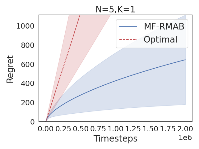
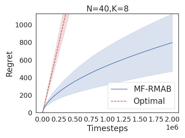
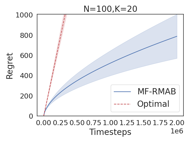
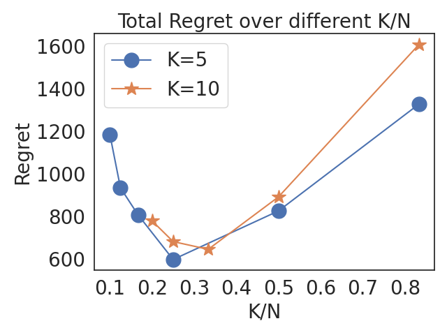
Figure 3. The first three plots show Regret vs. Time for different $K$ and $N$ settings on Synthetic-alternate dataset. The last plot shows the Regret with different $K/N$ values for $T\times H=2\times 10^{6}$ timesteps.

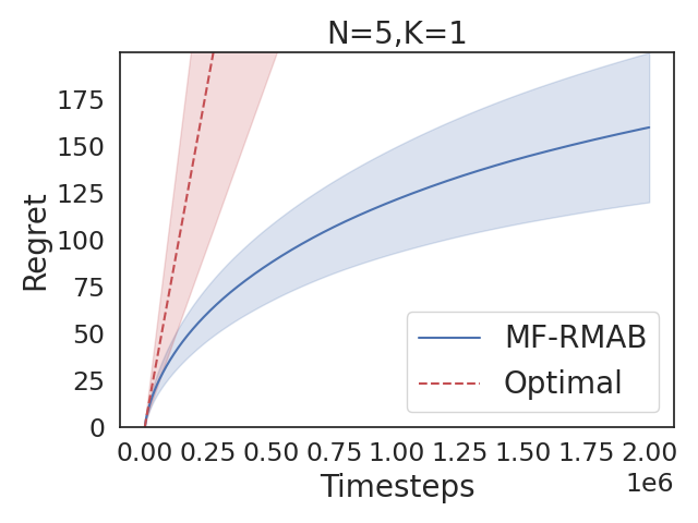
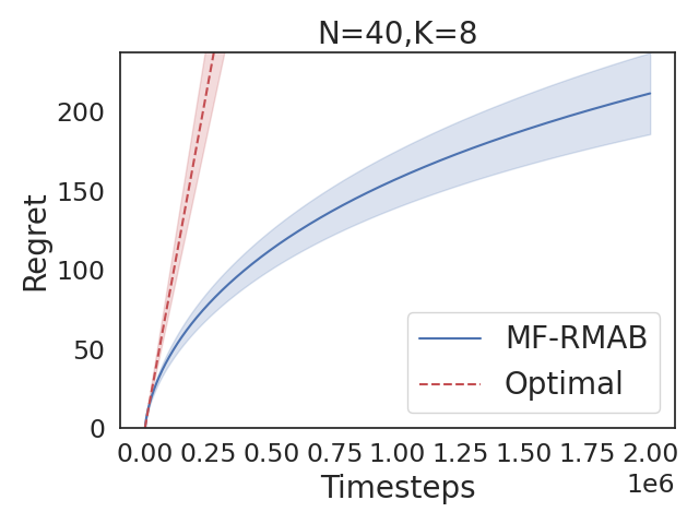
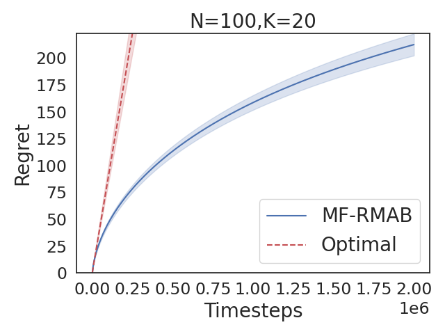
Figure 4. The first three plots show Regret vs. Time for different $K$ and $N$ settings on CPAP dataset. The last plot shows the Regret with different $K/N$ values for $T\times H=2\times 10^{6}$ timesteps.

Figure  1 shows the exposure arms get after 10k episodes on Synthetic dataset. Immediately, we can see the need for a fair policy, as Optimal tends to completely ignore sub-optimal arms, while MF-RMAB gives exposure proportional to the merit of the arms, and ensures fairness.

	Syn		Syn-alt		CPAP
	$G$	$t_{0}$	$G$	$t_{0}$	$G$	$t_{0}$
N=5 K=1	38	8	58	23	57	19
N=10 K=2	128	9	103	22	84	21
N=20 K=4	115	14	169	30	89	21
N=40 K=8	220	15	251	31	106	23
N=100 K=20	668	13	649	36	118	23

Table 1. Values of $G$ and $t_{0}$ on different datasets.

Table  1 shows the empirical values of $t_{0}$ and $G$ over the three datasets. We can see that while $t_{0}$ remains mostly consistent across different values of $N$ and $K$, $G$ varies significantly. This is because as $N$ increases, even if $K$ increases proportionally with $N$, the probability of some arm receiving a pull decreases, so $G_{i}$ can get very large for some arm in the worst case. As CPAP dataset is more homogeneous across arms as compared to the other two datasets, we see that the values of $G$ and $t_{0}$ are more uniform.

The first three plots of Figures  2, 3 and  4 show the various trends of fairness regret across the three datasets. We can see that MF-RMAB incurs a sublinear regret, while Optimal is unable to learn a fair policy and exhibits linear regret. As Synthetic and Synthetic-alternate datasets have a large amount of variance in the transition probabilities, we observe a large variance in regret as well.

The rightmost plot of Figures  2, 3 and  4 show the variation of total regret $FR^{T},T=10$k over increasing $\frac{K}{N}$ ratio. We can observe that in Synthetic and Synthetic-alternate datasets, the regret reaches its minimum around $\frac{K}{N}\approx 0.3$, while in CPAP dataset, the minima is around $\frac{K}{N}\approx 0.5$. Therefore, we conclude that increasing $K$ does not necessarily help in learning the transition probabilities faster, and can end up increasing the regret instead.

7. Conclusion/Future Work

We introduce exposure fairness to the online RMAB setting in the form of Merit Fair. We provide a sublinear bound on fairness regret in the single-pull case, and show that our algorithm MF-RMAB works admirably even in multiple-pull case. Future work could include formally defining a robust formulation of fairness regret for the multiple-pull case, along with provable sublinear regret bounds. Another possible research direction can be to define Fairness Regret using other possible reward formulations.

Appendix A MF-RMAB vs FaWT-Q

We now provide an empirical comparison with FaWT-Q Li and Varakantham (2022). The FaWT-Q algorithm implements the WIQL algorithm of Biswas et al. (2021) with the extra fairness contraint that each arm is pulled atleast $\eta$ number of times every $L$ timesteps. In accordance with the original work, we fix $\eta=2$ and vary $L=\{15,30,50\}$. For MF-RMAB, we vary the merit function $g(\mu)=e^{c\mu}$ with different values of $c$. Higher values of $L$ and $c$ means a more optimal algorithm, while lower values ensures more fairness. There is no reward penalty for violating the fairness constraints in FaWT-Q. We set $H=200$ and $T=1000$. As Li and Varakantham (2022) only provide results on Synthetic-alternate dataset, we run the simulations on the same. The results are averaged over 30 random seeds. The plots are shown in Figure 5.

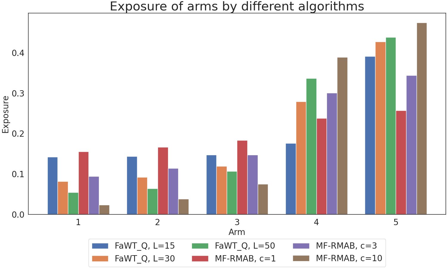
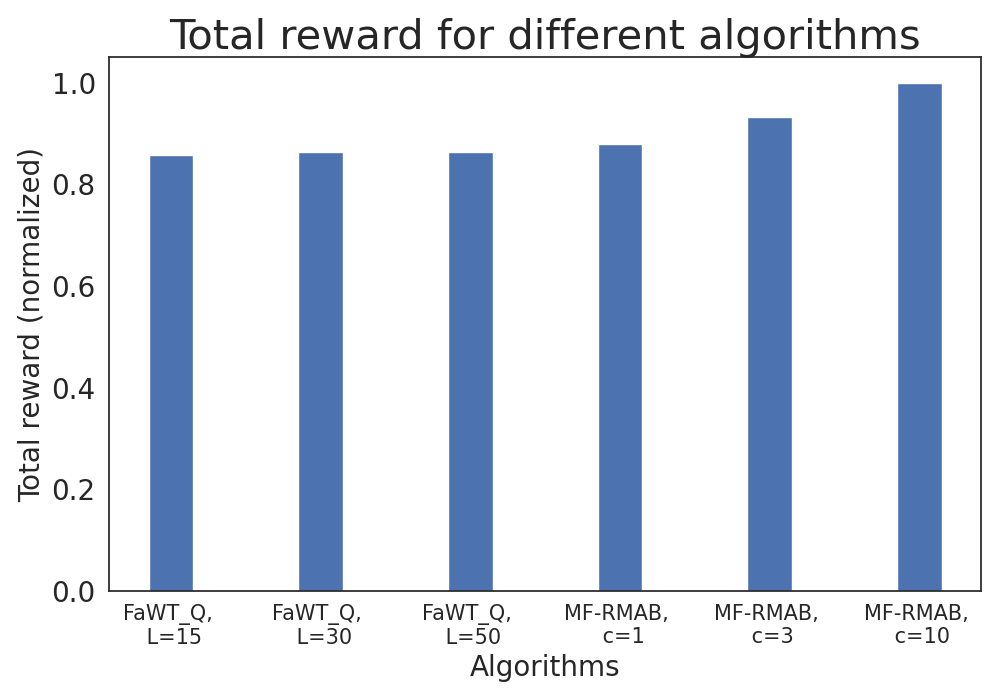
(a) $N=5$ and $K=1$

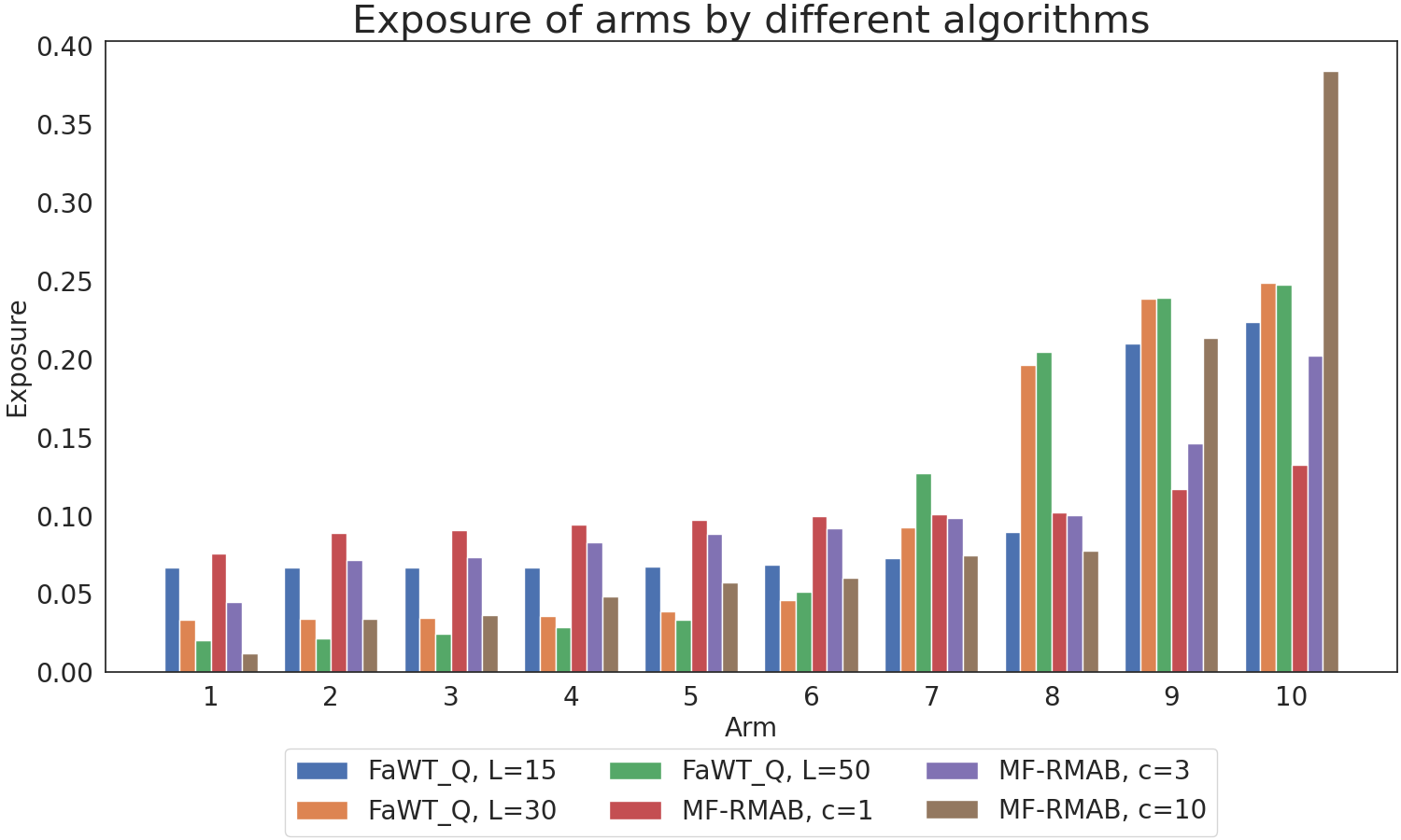
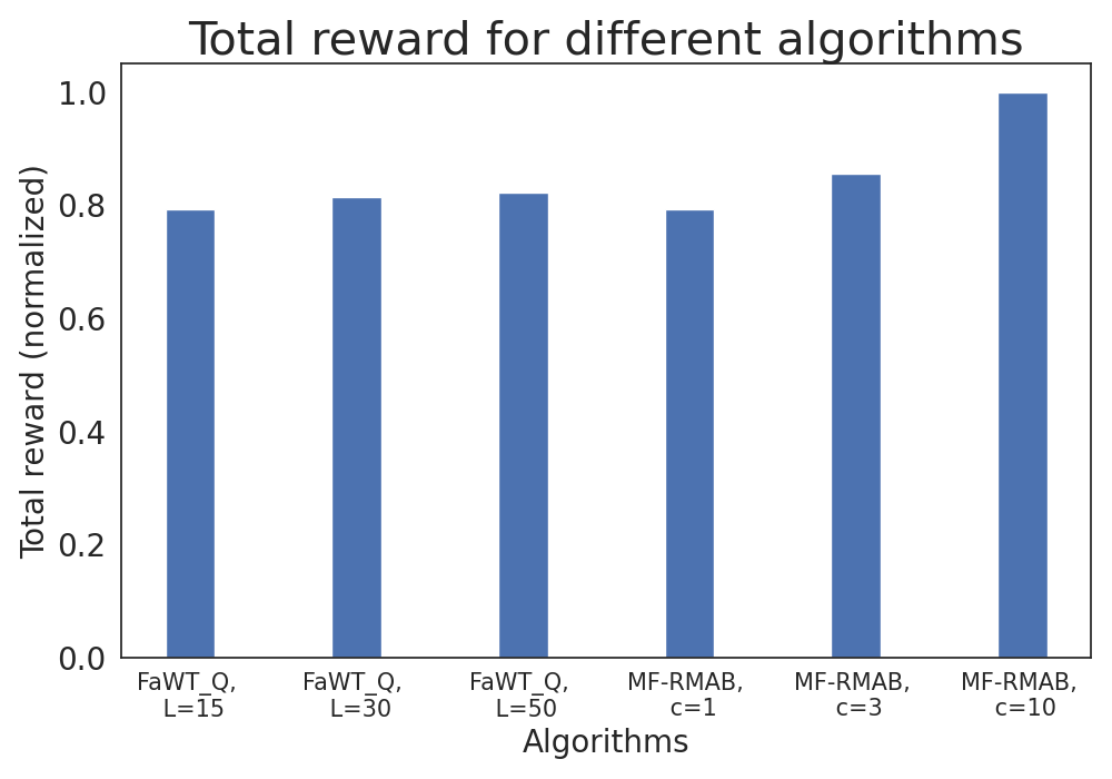
(b) $N=10$ and $K=2$

Figure 5. Comparison of MF-RMAB and FaWT-Q with respect to exposure and rewards. The y-axes are normalized to 1.

We can see that MF-RMAB provides a more egalitarian experience than FaWT-Q while performing equal or better in terms of reward. FaWT-Q tends to focus on the top few arms and ignores the rest, while MF-RMAB provides exposure to the worst arms as well. A very high value of $c$ makes the algorithm effectively optimal and thus offers little in terms of fairness.

Appendix B Additional Experiments

We explore the trends in fairness regret for different values of $c$ in the merit function $g(\mu)=e^{c\mu}$.

B.1. c=1

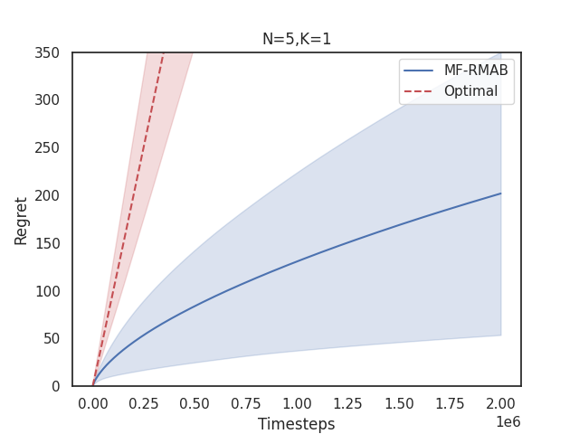
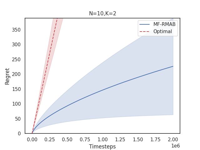
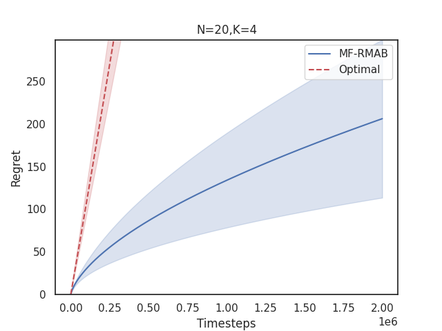
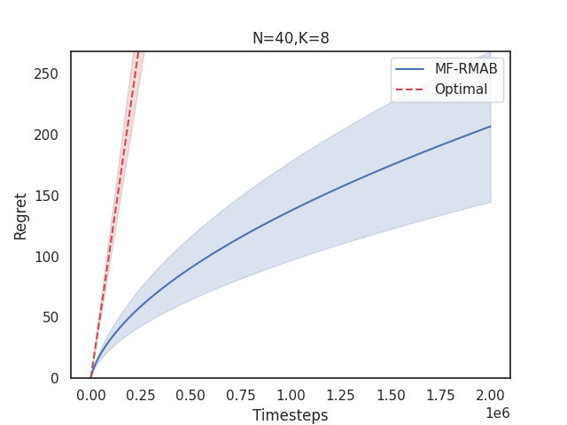
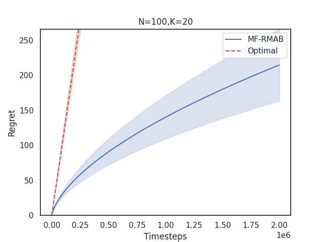
Figure 6. Fairness Regret on Synthetic dataset when $c=1$

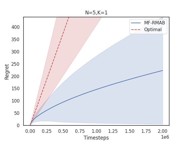
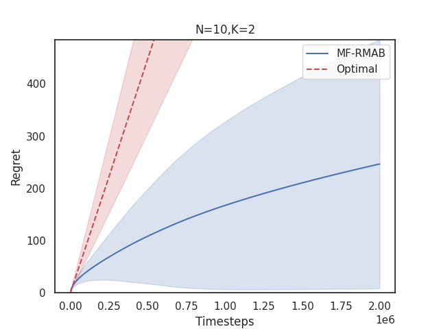
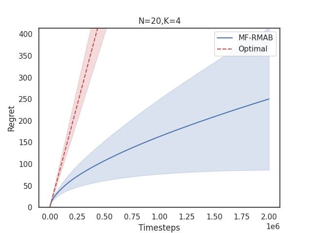
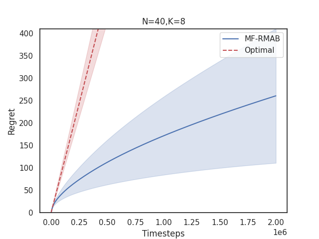
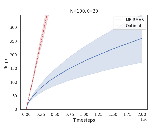
Figure 7. Fairness Regret on Synthetic-alternate dataset when $c=1$

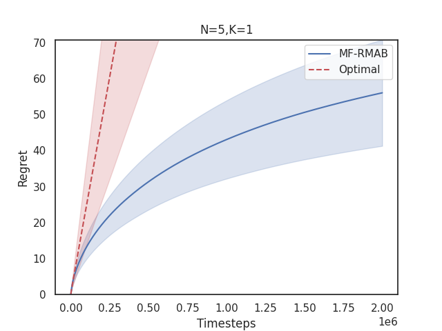
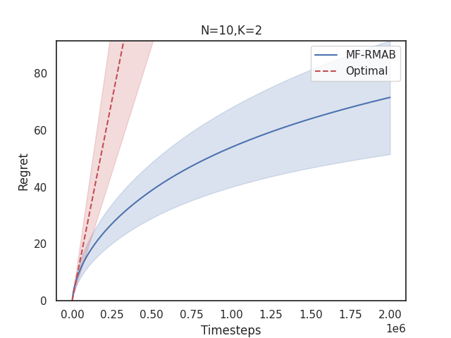
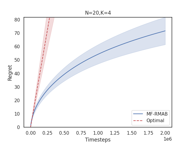
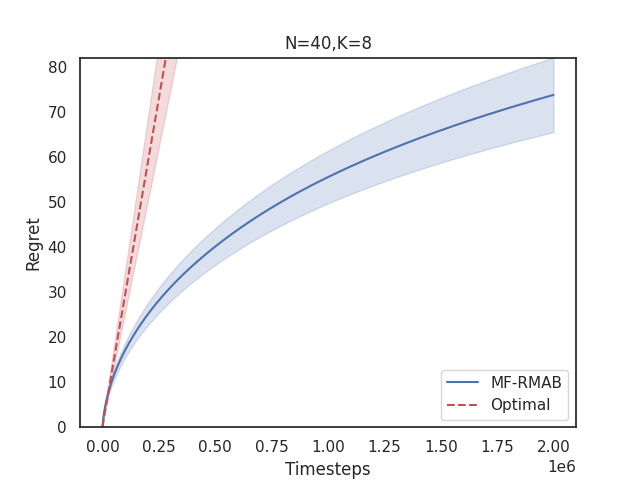
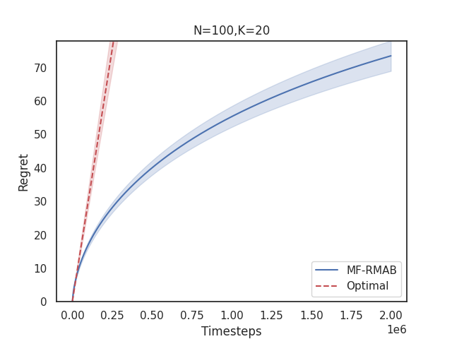
Figure 8. Fairness Regret on CPAP dataset when $c=1$

We observe from Figure 6, 7 and 8 that the value of $c$ directly influences the value of fairness regret. It is interesting to note that the variance has increased. A possible explanation is that a lower value of $c$ leads to less variation of the rewards of the arms, and it becomes more difficult to distinguish one arm from another, leading to higher variance in results.

B.2. c=10

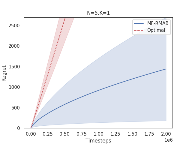
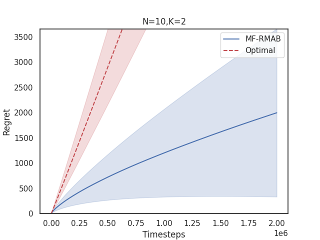
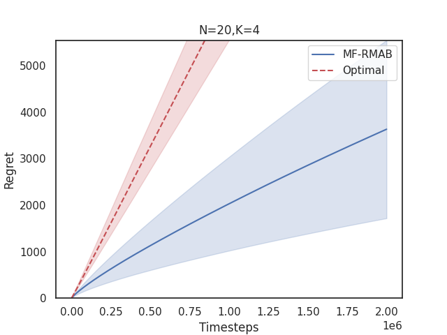
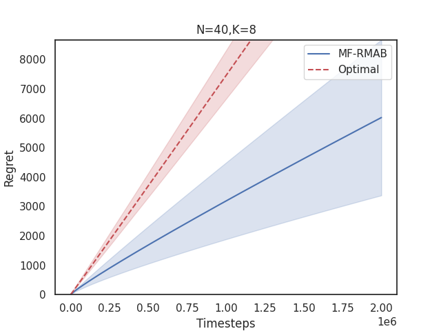
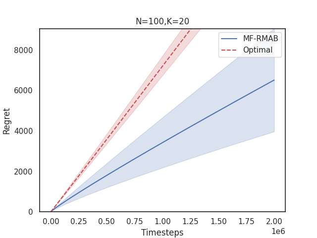
Figure 9. Fairness Regret on Synthetic dataset when $c=10$

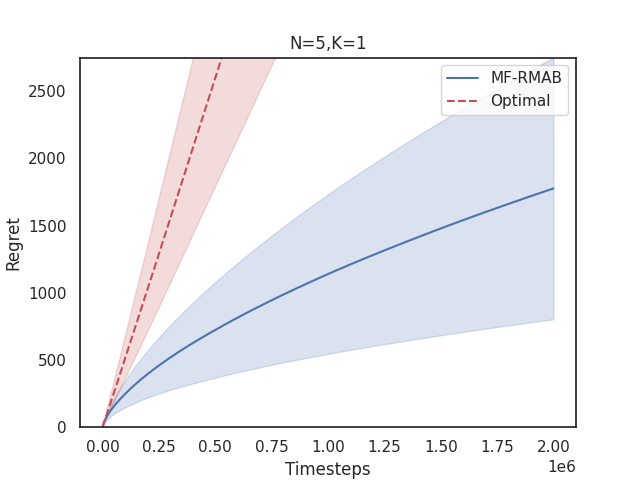
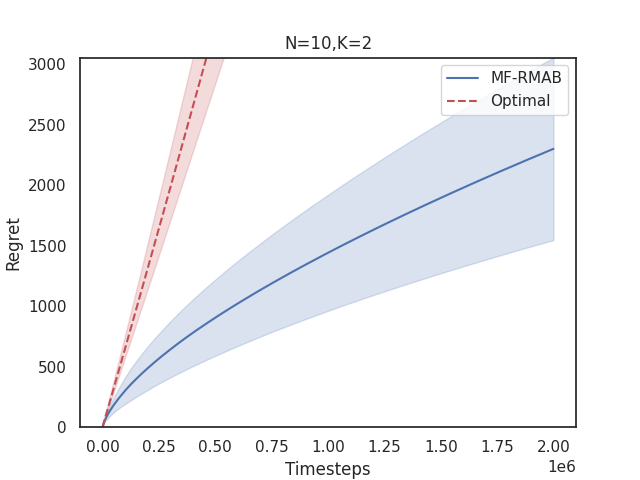
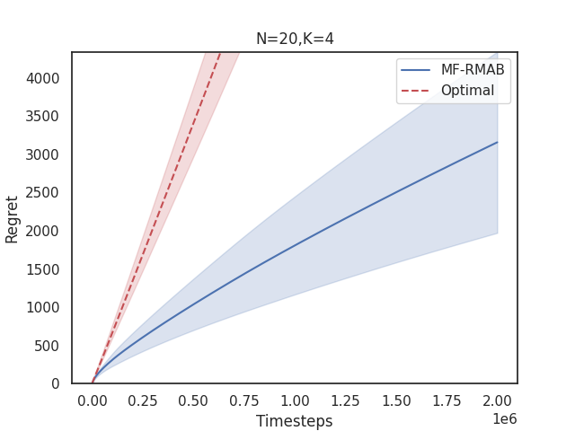
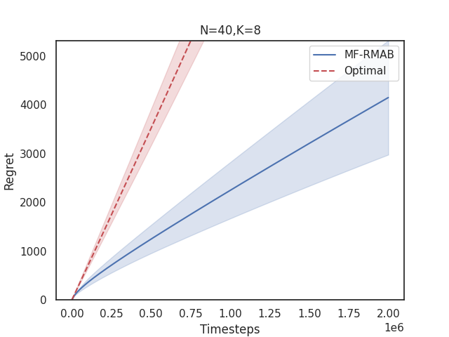
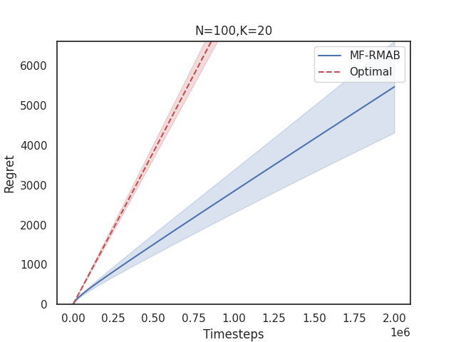
Figure 10. Fairness Regret on Synthetic-alternate dataset when $c=10$

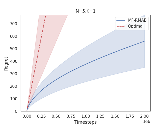
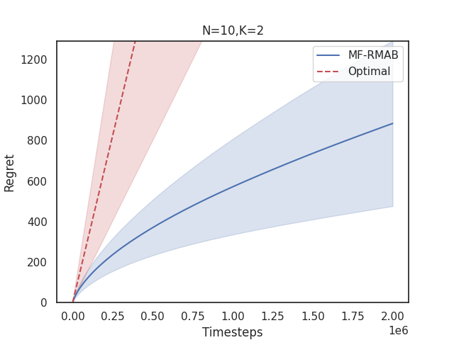
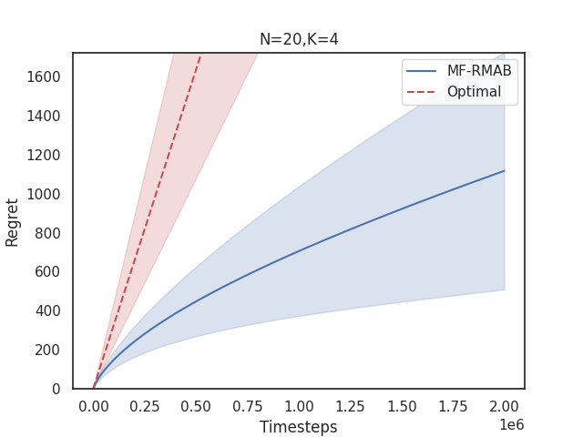
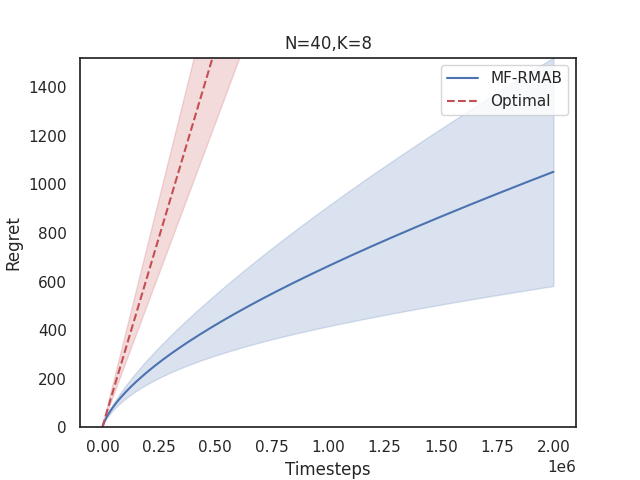
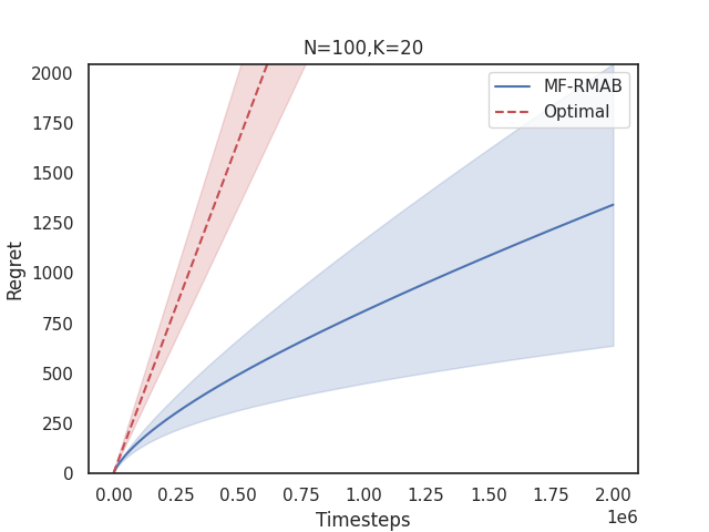
Figure 11. Fairness Regret on CPAP dataset when $c=10$

We observe from Figure 9, 10 and 11 that a higher $c$ leads to higher regret, and the regret curve becomes increasingly more linear. This is because $c$ is essentially a hyper-parameter that calibrates the trade-off between fairness and optimality. $c=0$ ensures uniform fairness across all arms, while a very high value of $c$ would result in a nearly optimal algorithm.

References

- (1)
- Abraham et al. (2013) Ittai Abraham, Omar Alonso, Vasilis Kandylas, and Aleksandrs Slivkins. 2013. Adaptive crowdsourcing algorithms for the bandit survey problem. In Conference on learning theory. PMLR, 882–910.
- Akbarzadeh and Mahajan (2019) Nima Akbarzadeh and Aditya Mahajan. 2019. Restless bandits with controlled restarts: Indexability and computation of Whittle index. In 2019 IEEE 58th conference on decision and control (CDC). IEEE, 7294–7300.
- Avrachenkov and Borkar (2022) Konstantin E Avrachenkov and Vivek S Borkar. 2022. Whittle index based Q-learning for restless bandits with average reward. Automatica 139 (2022), 110186.
- Berry and Fristedt (1985) Donald A Berry and Bert Fristedt. 1985. Bandit problems: sequential allocation of experiments (Monographs on statistics and applied probability). London: Chapman and Hall 5, 71-87 (1985), 7–7.
- Biswas et al. (2021) Arpita Biswas, Gaurav Aggarwal, Pradeep Varakantham, and Milind Tambe. 2021. Learn to intervene: An adaptive learning policy for restless bandits in application to preventive healthcare. arXiv preprint arXiv:2105.07965 (2021).
- Chen et al. (2020) Yifang Chen, Alex Cuellar, Haipeng Luo, Jignesh Modi, Heramb Nemlekar, and Stefanos Nikolaidis. 2020. Fair contextual multi-armed bandits: Theory and experiments. In Conference on Uncertainty in Artificial Intelligence. PMLR, 181–190.
- Fu et al. (2019) Jing Fu, Yoni Nazarathy, Sarat Moka, and Peter G Taylor. 2019. Towards q-learning the whittle index for restless bandits. In 2019 Australian & New Zealand Control Conference (ANZCC). IEEE, 249–254.
- Heidari and Krause (2018) Hoda Heidari and Andreas Krause. 2018. Preventing Disparate Treatment in Sequential Decision Making.. In IJCAI. 2248–2254.
- Herlihy et al. (2023) Christine Herlihy, Aviva Prins, Aravind Srinivasan, and John P Dickerson. 2023. Planning to fairly allocate: Probabilistic fairness in the restless bandit setting. In Proceedings of the 29th ACM SIGKDD Conference on Knowledge Discovery and Data Mining. 732–740.
- Hodge and Glazebrook (2015) David J Hodge and Kevin D Glazebrook. 2015. On the asymptotic optimality of greedy index heuristics for multi-action restless bandits. Advances in Applied Probability 47, 3 (2015), 652–667.
- Joseph et al. (2016) Matthew Joseph, Michael Kearns, Jamie H Morgenstern, and Aaron Roth. 2016. Fairness in learning: Classic and contextual bandits. Advances in neural information processing systems 29 (2016).
- Jung et al. (2019) Young Hun Jung, Marc Abeille, and Ambuj Tewari. 2019. Thompson sampling in non-episodic restless bandits. arXiv preprint arXiv:1910.05654 (2019).
- Jung and Tewari (2019) Young Hun Jung and Ambuj Tewari. 2019. Regret bounds for thompson sampling in episodic restless bandit problems. Advances in Neural Information Processing Systems 32 (2019).
- Kang et al. (2016) Yuncheol Kang, Amy M Sawyer, Paul M Griffin, and Vittaldas V Prabhu. 2016. Modelling adherence behaviour for the treatment of obstructive sleep apnoea. European journal of operational research 249, 3 (2016), 1005–1013.
- Killian et al. (2021a) Jackson A Killian, Arpita Biswas, Sanket Shah, and Milind Tambe. 2021a. Q-learning Lagrange policies for multi-action restless bandits. In Proceedings of the 27th ACM SIGKDD Conference on Knowledge Discovery & Data Mining. 871–881.
- Killian et al. (2023a) Jackson A Killian, Manish Jain, Yugang Jia, Jonathan Amar, Erich Huang, and Milind Tambe. 2023a. Equitable Restless Multi-Armed Bandits: A General Framework Inspired By Digital Health. arXiv preprint arXiv:2308.09726 (2023).
- Killian et al. (2023b) Jackson A Killian, Arshika Lalan, Aditya Mate, Manish Jain, Aparna Taneja, and Milind Tambe. 2023b. Adherence Bandits. (2023).
- Killian et al. (2021b) Jackson A Killian, Andrew Perrault, and Milind Tambe. 2021b. Beyond” to act or not to act”: Fast lagrangian approaches to general multi-action restless bandits. In Proceedings of the 20th International Conference on Autonomous Agents and MultiAgent Systems. 710–718.
- Li and Varakantham (2022) Dexun Li and Pradeep Varakantham. 2022. Efficient resource allocation with fairness constraints in restless multi-armed bandits. In Uncertainty in Artificial Intelligence. PMLR, 1158–1167.
- Li and Varakantham (2023) Dexun Li and Pradeep Varakantham. 2023. Avoiding Starvation of Arms in Restless Multi-Armed Bandits. In Proceedings of the 2023 International Conference on Autonomous Agents and Multiagent Systems. 1303–1311.
- Li et al. (2019) Fengjiao Li, Jia Liu, and Bo Ji. 2019. Combinatorial sleeping bandits with fairness constraints. IEEE Transactions on Network Science and Engineering 7, 3 (2019), 1799–1813.
- Mate et al. (2020) Aditya Mate, Jackson Killian, Haifeng Xu, Andrew Perrault, and Milind Tambe. 2020. Collapsing bandits and their application to public health intervention. Advances in Neural Information Processing Systems 33 (2020), 15639–15650.
- Mate et al. (2022) Aditya Mate, Lovish Madaan, Aparna Taneja, Neha Madhiwalla, Shresth Verma, Gargi Singh, Aparna Hegde, Pradeep Varakantham, and Milind Tambe. 2022. Field study in deploying restless multi-armed bandits: Assisting non-profits in improving maternal and child health. In Proceedings of the AAAI Conference on Artificial Intelligence, Vol. 36. 12017–12025.
- Mate et al. (2021) Aditya Mate, Andrew Perrault, and Milind Tambe. 2021. Risk-Aware Interventions in Public Health: Planning with Restless Multi-Armed Bandits.. In AAMAS. 880–888.
- Modi et al. (2019) Navikkumar Modi, Philippe Mary, and Christophe Moy. 2019. Transfer restless multi-armed bandit policy for energy-efficient heterogeneous cellular network. EURASIP Journal on Advances in Signal Processing 2019 (2019), 1–19.
- Ortner et al. (2012) Ronald Ortner, Daniil Ryabko, Peter Auer, and Rémi Munos. 2012. Regret bounds for restless markov bandits. In International conference on algorithmic learning theory. Springer, 214–228.
- Papadimitriou and Tsitsiklis (1994) Christos H Papadimitriou and John N Tsitsiklis. 1994. The complexity of optimal queueing network control. In Proceedings of IEEE 9th annual conference on structure in complexity Theory. IEEE, 318–322.
- Patil et al. (2021) Vishakha Patil, Ganesh Ghalme, Vineet Nair, and Yadati Narahari. 2021. Achieving fairness in the stochastic multi-armed bandit problem. The Journal of Machine Learning Research 22, 1 (2021), 7885–7915.
- Prins et al. (2020) Aviva Prins, Aditya Mate, Jackson A Killian, Rediet Abebe, and Milind Tambe. 2020. Incorporating Healthcare Motivated Constraints in Restless Bandit Based Resource Allocation. preprint (2020).
- Qian et al. (2016) Yundi Qian, Chao Zhang, Bhaskar Krishnamachari, and Milind Tambe. 2016. Restless poachers: Handling exploration-exploitation tradeoffs in security domains. In Proceedings of the 2016 International Conference on Autonomous Agents & Multiagent Systems. 123–131.
- Rothschild (1974) Michael Rothschild. 1974. A two-armed bandit theory of market pricing. Journal of Economic Theory 9, 2 (1974), 185–202.
- Wang et al. (2023) Kai Wang, Lily Xu, Aparna Taneja, and Milind Tambe. 2023. Optimistic whittle index policy: Online learning for restless bandits. In Proceedings of the AAAI Conference on Artificial Intelligence, Vol. 37. 10131–10139.
- Wang et al. (2021) Lequn Wang, Yiwei Bai, Wen Sun, and Thorsten Joachims. 2021. Fairness of exposure in stochastic bandits. In International Conference on Machine Learning. PMLR, 10686–10696.
- Weber and Weiss (1990) Richard R Weber and Gideon Weiss. 1990. On an index policy for restless bandits. Journal of applied probability 27, 3 (1990), 637–648.
- Whittle (1988) Peter Whittle. 1988. Restless bandits: Activity allocation in a changing world. Journal of applied probability 25, A (1988), 287–298.