Stable and Hurwitz slices, a degree principle
and a generalized Grace-Walsh-Szegő theorem

Abstract.

Univariate polynomials are called stable with respect to a circular region $\mathcal{A}$, if all of their roots are in $\mathcal{A}$. We consider the special case where $\mathcal{A}$ is a half-plane and investigate affine slices of the set of stable polynomials. In this setup, we show that an affine slice of codimension $k$ always contains a stable polynomial that possesses at most $2(k+2)$ distinct roots on the boundary and at most $(k+2)$ distinct roots in the interior of $\mathcal{A}$. This result also extends to affine slices of weakly Hurwitz polynomials, i.e. real, univariate, left half-plane stable polynomials. Subsequently, we apply these results to symmetric polynomials and varieties. Here we show that a variety described by polynomials in few multiaffine polynomials has no root in $\mathcal{A}^{n}$, if and only if it has no root in $\mathcal{A}^{n}$ with few distinct coordinates. This is at the same time a generalization of the degree principle to stable polynomials and a generalization of Grace-Walsh-Szegő’s coincidence theorem.

1. Introduction

The study of univariate polynomials whose roots are restricted to a subset of $\mathbb{C}$ is a central topic in mathematics. For instance, a univariate real polynomial is called hyperbolic if it is real rooted. Given a circular region $\mathcal{A}$ a univariate complex polynomial is said to be $\mathcal{A}$-stable if all its roots lie in $\mathcal{A}$. Since the roots of real polynomials come in conjugated pairs, hyperbolic polynomials are thus exactly real stable polynomials relative to the upper half-plane. Well-known examples of stable polynomials are Hurwitz stable polynomials, which are real open left half-plane stable polynomials, and Schur stable polynomials, which are unit disk stable polynomials. In particular, stable polynomials have been extensively leveraged to gain insights into combinatorial objects (see e.g. [4, 6, 8, 11]), and Hurwitz polynomials are at the heart of control theory and are used for asymptotic stability for linear continuous-time systems (see e.g., [17] or [7, p. 75]).

Studying the roots of univariate polynomials is deeply related to studying multivariate symmetric polynomials by the Vieta formula

$$\prod_{i=1}^{n}(T-x_{i})=T^{n}-e_{1}(x)T^{n-1}+e_{2}(x)T^{n-2}+\ldots+(-1)^{n}e_{n}(x)$$

where $e_{k}=\sum_{I\subset[n],|I|=k}\prod_{i\in I}X_{i}$ denotes the $k$-th elementary symmetric polynomial. In the paper we associate points $z\in\mathbb{C}^{n}$ with monic polynomials

$$f_{z}=T^{n}-z_{1}T^{n-1}+z_{2}T^{n-2}-\ldots+(-1)^{n}z_{n}.$$

In particular, monic hyperbolic polynomials are described by the image of $\mathbb{R}^{n}$ under the Vieta map, i.e., the image under the evaluation of the $n$ elementary symmetric polynomials. Similarly to this hyperbolic picture, monic $A$-stable polynomials can be identified with the image of $\mathcal{A}^{n}$ under the Vieta map.

Sets of hyperbolic polynomials obtained by fixing the first $k$ coefficients have been considered by various authors, beginning with the work of Arnold [2, 9, 14, 18] and recently [16, 20]. In the domain of the Vieta map, such sets are called Vandermonde varieties, whereas the corresponding sets in the image of the Vieta map are called hyperbolic slices. More generally, this notion has been introduced in [21] to sets of hyperbolic polynomials that are cut out by a $(n-k)$-dimensional affine subspace. A remarkable property of such hyperbolic slices concerns their local extreme points: It turns out that these local extreme points of linear functionals can be characterized as polynomials with at most $k$ distinct roots. Similarly to this hyperbolic situation, we study affine slices of the set of upper half-plane stable polynomials defined by $k$ linear combinations of coefficients and show in Theorem 2.4 that the local extreme points of such stable slices have at most $k$ non-real roots and at most $2k$ distinct real roots.

One of our main motivations for this result is provided by a natural connection to the classical Grace-Walsh-Szegő’s coincidence theorem. This beautiful result states that for a symmetric multiaffine polynomial $f\in\mathbb{C}[\underline{X}]$ evaluated on a circular region $\mathcal{A}\subset\mathbb{C}$ there exists for all $(\zeta_{1},\ldots,\zeta_{n})\in\mathcal{A}^{n}$ some $\zeta\in\mathcal{A}$ with the property that $f(\zeta_{1},\ldots,\zeta_{n})=f(\zeta,\ldots,\zeta)$, under the assumption that the degree of $f$ is $n$ or $\mathcal{A}$ is convex. The coincidence theorem has several applications in stability testing since it allows reduction of the question of verifying multivariate stability to univariate polynomials. However, the assumptions of the theorem are relatively strict. It was proven by Brändén and Wagner [5] that no analogous result can be applied to any multiaffine polynomials invariant under a fixed proper permutation subgroup of $S_{n}$. We use our results on stable slices and the connection with symmetric polynomials to prove in Theorem 4.6 and Corollary 4.11 a Grace-Walsh-Szegő-like theorem for multivariate polynomials which can be written as a polynomial in few multiaffine symmetric polynomials when $\mathcal{A}$ is a half-plane. We show that for any point $\zeta\in\mathcal{A}^{n}$, we can find a point with few distinct coordinates and the same evaluation. Furthermore, in a similar spirit, we prove a double-degree principle for stable varieties in Corollary 4.8 and also a half-degree principle for the upper half-plane in Theorem 4.13. Our results on stable slices do not transfer directly to Hurwitz slices since the coefficients of those polynomials are real. However, we prove that if we fix $k$ linear combinations of coefficients of a weakly Hurwitz polynomial, then there is a weakly Hurwitz polynomial satisfying the same relations and having only $k$ roots with negative real part and $2k$ distinct roots with real part equal to zero (see Theorem 3.3).

Structure of the article

In Section 2 we study stable slices of univariate polynomials and show in particular that local extreme points of stable slices correspond to polynomials with few distinct roots (Theorem 2.4). In Section 3 we study Hurwitz slices and their boundary by root multiplicities. In Section 4 we apply our results from Section 2 to multivariate symmetric polynomials and formulate a double-degree principle for stable polynomials and our generalization of Grace-Walsh-Szegő’s coincidence theorem (Theorem 4.6, Corollaries 4.8 and 4.11). Finally, we formulate open questions.

2. Stable slices

Throughout the article we denote by $\mathbb{C}[T]$ and $\mathbb{R}[T]$ the rings of univariate complex and real polynomials and $k\leqslant n$ be fixed positive integers. For a complex number $x$ we write $\operatorname{Re}(x)$ and $\operatorname{Im}(x)$ for its real and imaginary parts. Furthermore, we commonly identify the set of monic univariate polynomials with $\mathbb{C}^{n}$ via the bijection

$$(z_{1},\dots,z_{n})\longmapsto T^{n}-z_{1}T^{n-1}+z_{2}T^{n-2}-\dots+(-1)^{n}z_{n}.$$

In this section, we study univariate stable polynomials, i.e. polynomials that have all their roots lying in a half-plane. In particular, we are interested in intersections of the set of stable polynomials with affine subspaces of $\mathbb{C}^{n}$. As multiplication with units in $\mathbb{C}$ does not change the roots of a polynomial, we restrict to monic stable polynomials. We denote the closed upper half-plane by $\mathbb{H}_{+}$, i.e.

$$\mathbb{H}_{+}=\{x\in\mathbb{C}\leavevmode\nobreak\ |\leavevmode\nobreak\ \operatorname{Im}(x)\geq 0\}$$

Definition 2.1.

Let $\mathbb{H}$ be a closed half-plane. We denote by

$$\mathcal{S}_{\mathbb{H}}:=\left\{z\in\mathbb{C}^{n}\leavevmode\nobreak\ \middle|\leavevmode\nobreak\ T^{n}-z_{1}T^{n-1}+\dots+(-1)^{n}z_{n}\text{ has all roots in $\mathbb{H}$}\right\}$$

the set of monic $\mathbb{H}$-stable polynomials of degree $n$. Furthermore, we define

$$\mathbb{H}_{k,m}:=\left\{x\in\mathbb{H}^{n}\leavevmode\nobreak\ \middle|\leavevmode\nobreak\ |\{x_{1}\dots,x_{n}\}\cap\partial\mathbb{H}|\leqslant k\text{ and }|\{i\in\{1,\dots,n\}\leavevmode\nobreak\ |\leavevmode\nobreak\ x_{i}\in\mathring{\mathbb{H}}\}|\leqslant m\right\}$$

the set of points with at most $k$ distinct coordinates on the boundary of $\mathcal{A}$ and at most $m$ coordinates in the interior of $\mathbb{H}$. The set of all polynomials with all roots in $\mathbb{H}_{k,m}$ is

$$\mathcal{S}_{\mathbb{H}}^{k,m}:=\left\{z\in\mathcal{S}_{\mathbb{H}}\leavevmode\nobreak\ \middle|\leavevmode\nobreak\ T^{n}-z_{1}T^{n-1}+\dots+(-1)^{n}z_{n}\text{ has roots }(x_{1},\ldots,x_{n})\in\mathbb{H}_{k,m}\right\}.$$

For $a=(a_{1},\dots,a_{k})\in\mathbb{C}^{k}$ and a surjective linear map $L:\leavevmode\nobreak\ \mathbb{C}^{n}\to\mathbb{C}^{k}$ we define the affine slice

$$\mathcal{S}_{\mathbb{H}}\cap L^{-1}(a)=\left\{z\in\mathcal{S}_{\mathbb{H}}\leavevmode\nobreak\ \middle|\leavevmode\nobreak\ L(z)=a\right\}\text{ and }S_{\mathbb{H}}^{k,m}\cap L^{-1}(a)=\left\{z\in\mathcal{S}_{\mathbb{H}}^{k,m}\leavevmode\nobreak\ \middle|\leavevmode\nobreak\ L(z)=a\right\}.$$

A set of the form $\mathcal{S}_{\mathbb{H}}\cap L^{-1}(a)$ is called a $\mathbb{H}$-stable slice. If $\mathbb{H}=\mathbb{H}_{+}$ is the upper half-plane, we write $\mathcal{S}$ for $\mathcal{S}_{\mathbb{H}_{+}}$.

Remark 2.2.

Notice that the set $\mathcal{S}_{\mathbb{H}}$ can be identified with a semi-algebraic set in $\mathbb{R}^{2n}$. In contrast to the set of hyperbolic polynomials, where an explicit description of the set of hyperbolic polynomials in terms of the coefficients can be obtained via Sturm’s Theorem, it seems in general not easy to give an explicit description of $\mathcal{S}_{\mathbb{H}}$. However, in the case of polynomials with real coefficients, this is possible and we will expose this case in in Section 3.

The assumption that $L$ is surjective is only for convenience in the notation (see Remark 2.5). It suffices to study stable slices of a fixed half-plane. This follows since translations and rotations are linear isomorphisms. Let $\phi:\mathbb{H}\to\mathbb{G}$ be a linear bijection between half-planes and let $\psi=\phi^{-1}$ be its inverse. Then $f_{z}\in\mathcal{S}_{\mathbb{H}}$ if and only if $f_{z}\circ\psi\in\mathcal{S}_{\mathbb{G}}$. In particular, we can restrict to $\mathbb{H}_{+}$-stable slices.

Definition 2.3.

Let $A\subset\mathbb{C}^{n}$ and let $z\in A$. We say that $z$ is a local extreme point of $A$ if there is a neighborhood $U$ of $z$ such that $z$ is an extreme point of $\operatorname{conv}(A\cap U)$.

Like the set of extreme points of a set $A$ is the set of global minima of linear functions, the set of local extreme points of $A$ is the set of local minima of linear functions.

The following theorem which is a generalization of [20, Theorem 4.2] and [21, Theorem 2.8], is our main result on stable slices characterizing local extreme points. As a corollary, we obtain a result for arbitrary stable slices in Corollary 2.10.

Theorem 2.4.

The local extreme points of an $\mathbb{H}_{+}$-stable slice $\mathcal{S}\cap L^{-1}(a)$ correspond to polynomials that have at most $k$ roots in $\mathbb{H}_{+}\setminus{\mathbb{R}}$ and at most $2k$ distinct real roots.

In other words, any local extreme point of the $\mathbb{H}_{+}-$stable slice $\mathcal{S}\cap L^{-1}(a)$ is contained in the set $\mathcal{S}^{2k,k}$. In the proof, we investigate the multiplicity of the roots of polynomials in the stable slice.

Proof.

Let $z\in\mathcal{S}\cap L^{-1}(a)$ be a local extreme point, i.e., there is a neighborhood $U$ of $z$ such that $z$ is an extreme point of $\operatorname{conv}(\mathcal{S}\cap L^{-1}(a)\cap U)$. Consider $f:=T^{n}-z_{1}T^{n-1}+\dots+(-1)^{n}z_{n}$ and factor $f=p\cdot r$, where $p$ has only roots in $\mathbb{H}_{+}\setminus{\mathbb{R}}$ and $r$ has only real roots.

1. We show first that $p$ has at most $k$ roots, i.e., $\deg p\leqslant k$. We assume that $\deg p:=m>k$ and want to find a contradiction. Write $r=T^{n-m}+r_{1}T^{n-m-1}+\dots+r_{n-m}$ and define $r_{0}:=1$ and consider the linear map

   $$\begin{array}[]{rcccc}\chi&:&\mathbb{C}^{m}&\,\,\longrightarrow&\mathbb{C}^{n}\\[2.15277pt] &&y&\longmapsto&\left(\sum_{i+j=1}r_{i}y_{j},\dots,\sum_{i+j=n}r_{i}y_{j}\right)\end{array}.$$

   Since $m>k$, there is $b\in\ker(L\circ\chi)\setminus\{0\}$. We define $h:=b_{1}T^{m-1}+\dots+b_{m}$ and $g:=h\cdot r=c_{1}T^{n-1}+\ldots+c_{n}\neq 0$, where $c=\chi(b)$ by construction and therefore $c\in\ker L$. Now, because $p$ has only roots in $\mathbb{C}\setminus{\mathbb{R}}$, $p\pm\varepsilon h$ is stable for $\varepsilon>0$ small enough, sicne the roots depend continuously on the coefficients [10]. Hence

   $$(p\pm\varepsilon h)\cdot r=f\pm\varepsilon h\cdot r=f\pm\varepsilon g$$

   is stable for all $\varepsilon>0$ small enough, i.e., $z\pm\varepsilon c\in\mathcal{S}\cap L^{-1}(a)$. If we choose $\varepsilon>0$ small enough we can ensure also that $z\pm\varepsilon c\in U$. But then

   $$z=\frac{z+\varepsilon c+z-\varepsilon c}{2},$$

   a contradiction to $z$ being an extreme point of $\operatorname{conv}(\mathcal{S}\cap L^{-1}(a)\cap U)$.

2. Now we show that $r$ has at most $2k$ distinct roots. We assume $r$ has distinct roots $x_{1},\dots,x_{m}$ where $m>2k$ and want to find a contradiction. We factor $f$ as follows:

   $$f=\underbrace{\prod_{i=1}^{m}(T-x_{i})}_{=:q}\cdot s,$$

   where $s$ is of degree $n-m$. Write $s=T^{n-m}+s_{1}T^{n-m-1}+\dots+s_{n-m}$ and define $s_{0}:=1$ and consider the linear map

   $$\begin{array}[]{rcccc}\chi&:&\mathbb{R}^{m}&\,\,\longrightarrow&\mathbb{C}^{n}\\[2.15277pt] &&y&\longmapsto&\left(\sum_{i+j=1}s_{i}y_{j},\dots,\sum_{i+j=n}s_{i}y_{j}\right)\end{array}.$$

   Since $m>2k$, there is $b\in\ker(L\circ\chi)\setminus\{0\}$. We define $h:=b_{1}T^{m-1}+\dots+b_{m}$ and $g:=h\cdot s=c_{1}T^{n-1}+\ldots+c_{n}\neq 0$, where $c=\chi(b)$ by construction and therefore $c\in\ker L$. Now, because $q$ has only single roots in $\mathbb{R}$, $q\pm\varepsilon h$ is stable for $\varepsilon>0$ small enough, since the roots depend continuously on the coefficients and complex roots come as conjugated pairs (see e.g. [10]). Hence

   $$(q\pm\varepsilon h)\cdot s=f\pm\varepsilon\cdot g$$

   is stable for all $\varepsilon>0$ small enough, i.e., $z\pm\varepsilon c\in\mathcal{S}\cap L^{-1}(a)$. If we choose $\varepsilon>0$ small enough we can ensure also that $z\pm\varepsilon c\in U$. But then

   $$z=\frac{z+\varepsilon c+z-\varepsilon c}{2},$$

   a contradiction to $z$ being an extreme point of $\operatorname{conv}(\mathcal{S}\cap L^{-1}(a)\cap U)$.

∎

Remark 2.5.

The assumption that $L$ is surjective is only for convenience. In particular, if $L$ is not surjective one obtains the same result as in Theorem 2.4, where $k$ can be replaced by $\operatorname{rank}L.$

We point out that the converse of Theorem 2.4 is not true, i.e. not every point $z\in\mathcal{S}^{2k,k}\cap L^{-1}(a)$ is a local extreme point.

Example 2.6.

Let $n=3$, $k=1$ and

$$\begin{array}[]{rcccc}L&:&\mathbb{C}^{3}&\,\,\longrightarrow&\mathbb{C}\\[2.15277pt] &&(z_{1},z_{2},z_{3})&\longmapsto&z_{3}\end{array}.$$

Then $(i,0,0)\in\mathcal{S}^{2k,k}\cap L^{-1}(0),$ but

$$(i,0,0)=\frac{(0,0,0)+(2i,0,0)}{2}$$

is not a local extreme point since $(0,0,0),(2i,0,0)\in\mathcal{S}\cap L^{-1}(0)$.

We consider the set of stable polynomials of degree $n$ with fixed first coefficients which is an instance of a stable slice.

Definition 2.7.

For an integer $k\geq 1$ and a point $a=(a_{1},\ldots,a_{k})\in\mathbb{C}^{k}$ we define $\mathcal{S}(a)=\mathcal{S}\cap\{z\in\mathbb{C}^{n}|z_{1}=a_{1},\ldots,z_{k}=a_{k}\}$ as the set of all monic $\mathbb{H}_{+}$-stable polynomials of degree $n$ whose first $k$ non-trivial coefficients are determined by the point $a$.

With our previous notation we have $\mathcal{S}(a)=S\cap L^{-1}(a)$ where $L:\leavevmode\nobreak\ \mathbb{C}^{n}\to\mathbb{C}^{k}$ denotes the projection to the first $k$ coordinates.

Lemma 2.8.

For an integer $k\geq 2$ the stable slice $\mathcal{S}(a)$ is compact.

Proof.

As the empty set is compact we can assume that there is $z\in\mathcal{S}(a)$. Furthermore we denote by $x=(x_{1},\dots,x_{n})\in\mathbb{H}_{+}$ the roots of the polynomial

$$f_{z}:=T^{n}-z_{1}T^{n-1}+\cdots+(-1)^{n}z_{n}.$$

Then, if $e_{1}$ and $e_{2}$ denote the first and second elementary symmetric polynomial

$$\sum_{i=1}^{n}x_{i}=e_{1}(x)=a_{1}$$

and hence the imaginary part of the $x_{i}^{\prime}s$ is contained in $[0,\operatorname{Im}(a_{1})]$. Furthermore

$$\sum_{i=1}^{n}x_{i}^{2}=e_{1}(x)^{2}-2e_{2}(x)=a_{1}^{2}-2a_{2}$$

and hence

$$\sum_{i=1}^{n}\operatorname{Re}(x_{i})^{2}=\sum_{i=1}^{n}\operatorname{Re}(x_{i}^{2})+\operatorname{Im}(x_{i})^{2}\leqslant\sum_{i=1}^{n}\operatorname{Re}(x_{i}^{2})+\operatorname{Im}(a_{1})^{2}=\operatorname{Re}\left(\sum_{i=1}^{n}x_{i}^{2}\right)+n\operatorname{Im}(a_{1})^{2}\leavevmode\nobreak\ .$$

Since $\sum_{i=1}^{n}x_{i}^{2}=a_{1}^{2}-a_{2}$ we have

$$\sum_{i=1}^{n}\operatorname{Re}(x_{i})^{2}\leqslant\operatorname{Re}(a_{1}^{2}-2a_{2})+n\operatorname{Im}(a_{1})^{2}\leavevmode\nobreak\ .$$

This shows that also the real part of the $x_{i}^{\prime}s$ is bounded. Thus the set $\mathcal{S}(a)$ is bounded. Furthermore, as the roots of a polynomial depend continuously on the coefficients it is clear that $\mathcal{S}(a)$ is closed and therefore compact. ∎

Remark 2.9.

For a surjective linear map $L:\leavevmode\nobreak\ \mathbb{C}^{n}\to\mathbb{C}^{k}$ and $a\in\mathbb{C}^{k}$ we can have that the set $\mathcal{S}\cap L^{-1}(a)$ is unbounded. Then we consider the linear map $\widetilde{L}:\leavevmode\nobreak\ \mathbb{C}^{n}\to\mathbb{C}^{k+2}$, where $\widetilde{L}(z)=(L(z),z_{1},z_{2})$. The set $\mathcal{S}_{\mathbb{H}_{+}}\cap\widetilde{L}^{-1}(b)$ is compact for any point $b\in\mathbb{C}^{k+2}$, by a similar argument as in the proof of Lemma 2.8. Moreover, if one or both of the first two unit vectors are in the row span of a matrix representation of $L$, then we can consider $\widehat{L}(z)=(L(z),z_{i})$ for $i\in\{1,2\}$ instead of $L$ or the original stable slice was already compact.

We are now ready to present our main result on general half-plane stable slices.

Corollary 2.10.

Let $\mathbb{H}$ be a closed half-plane. Any non-empty $\mathbb{H}$-stable slice $\mathcal{S}_{\mathbb{H}}\cap L^{-1}(a)\neq\emptyset$ contains a point that corresponds to a polynomial with at most $k+2$ roots in $\mathring{\mathbb{H}}$ and at most $2(k+2)$ distinct roots in $\partial\mathbb{H}$, i.e.

$$\mathcal{S}^{2(k+2),k+2}_{\mathbb{H}}\cap L^{-1}(a)\neq\emptyset.$$

Proof.

Since $\mathbb{H}$ can be bijectively mapped to $\mathbb{H}_{+}$ under a linear isomorphism it suffices to show the theorem for $\mathbb{H}=\mathbb{H}_{+}$. Now the claim follows from Theorem 2.4, Lemma 2.8 and Remark 2.9. ∎

Corollary 2.10 says that stable slices do always contain a point with few distinct zeros. Moreover, we can characterize the maximal number of distinct roots on the boundary of the half-plane and the number of distinct roots in the interior. We point out that the result is independent of the degree $n$ and is more import if the degree is large. In particular, we observe a stabilization in the structure of local extreme points of stable slices if there are at least $n\geq 3k$ variables.

Remark 2.11.

In the case that $L$ is the projection to the first $k<n$ coordinates, we can replace $2k$ by $k$ in Theorem 2.4 since $(0,\ldots,0,1)\in\ker(L\circ\chi)$. This follows because one can choose $h=1$ in the proof in this case. Furthermore, if $k\geq 2$ the stable slice is compact in this case by Lemma 2.8. So we can exchange $\mathcal{S}^{2(k+2),k+2}_{\mathbb{H}}\cap L^{-1}(a)$ by $\mathcal{S}^{k,k}_{\mathbb{H}}\cap L^{-1}(a)$ in Corollary 2.10.

One could hope that every stable slice contains also points that correspond to polynomials with $k$ distinct roots in $\mathbb{H}_{+}$, analogous to the case of compact hyperbolic slices, mentioned in [21, Theorem 2.8]. The next example shows that this is not true in general even when $L$ is the projection to the first $k$ coordinates.

Example 2.12.

We consider $\mathcal{S}\cap L^{-1}(a)$, where

$$a:=(-23i,-463,8461i)\quad\text{and}\quad\begin{array}[]{rcccc}L&:&\mathbb{C}^{4}&\,\,\longrightarrow&\mathbb{C}^{3}\\[2.15277pt] &&(z_{1},z_{2},z_{3},z_{4})&\longmapsto&(z_{1},z_{2},z_{3})\end{array}$$

is the projection to the first $3$ coordinates. Then $\mathcal{S}\cap L^{-1}(a)$ is non-empty, since

$$(-23i,-463,8461i,8020)\in\mathcal{S}\cap L^{-1}(a).$$

The coefficient vector corresponds to a polynomial with roots $-20+i,i,20+i$ and $20i$. Furthermore, $\mathcal{S}\cap L^{-1}(a)$ contains no point corresponding to a polynomial with at most $3$ distinct roots.

Figure 1. The stable slice $\mathcal{S}_{\mathbb{H}_{+}}\cap L^{-1}(a)$

3. Hurwitz slices

In this section we consider Hurwitz polynomials, i.e. real univariate polynomials with all roots in the left half-plane. Moreover, polynomials with all roots having nonpositive real part are called weakly Hurwitz. We show in Theorem 3.3 that the local extreme points of affine slices of the set of monic Hurwitz polynomials have few distinct roots and study a partial order on the set of monic Hurwitz polynomials in Subsection 3.2.

Like for stable polynomials we identify monic weakly Hurwitz polynomials with their coefficients. Any monic weakly Hurwitz polynomial has nonnegative coefficients.

Similary to hyperbolic polynomials, monic Hurwitz polynomials can be characterized as poynomials with a positive definite finite Hurwitz matrix [12]. While the finite Hurwitz matrix of any weakly Hurwitz polynomial is positive semidefinite, its converse is not true (see [3]). Kemperman [13] showed that weakly Hurwitz polynomials can be characterized in a similar way by their infinite Hurwitz matrix (see also [1, Thm. 4.9] for another characterization).

3.1. Hurwitz slices and their local extreme points.

In contrast to the study of stable polynomials in Section 2 where we considered surjective linear maps $\mathbb{C}^{n}\to\mathbb{C}^{k}$ over the field $\mathbb{C}$, we restrict to real linear maps over $\mathbb{R}$. However, since the roots of weakly Hurwitz polynomials can be complex, we cannot directly apply any result about hyperbolic polynomials.

Definition 3.1.

We write $\mathbb{H}_{\text{left}}$ for the left half-plane in $\mathbb{C}$, i.e.

$$\mathbb{H}_{\text{left}}:=\left\{x\in\mathbb{C}^{n}\leavevmode\nobreak\ \middle|\leavevmode\nobreak\ \operatorname{Re}(x)\leqslant 0\right\}$$

The set of monic weakly Hurwitz polynomials is defined by

$$\mathcal{H}\mathcal{W}:=\mathcal{S}_{\mathbb{H}_{\text{left}}}\cap\mathbb{R}^{n}:=\left\{z\in\mathbb{R}^{n}\leavevmode\nobreak\ \middle|\leavevmode\nobreak\ f_{z}\text{ has all roots in }\mathbb{H}_{\text{left}}\right\}.$$

Moreover, for a linear map $L:\leavevmode\nobreak\ \mathbb{R}^{n}\to\mathbb{R}^{k}$ we call the set $\mathcal{H}\mathcal{W}\cap L^{-1}(a)$ a Hurwitz slice.

We have the following connection between Hurwitz polynomials and stable polynomials.

Remark 3.2.

The set of monic weakly Hurwitz polynomials $\mathcal{H}\mathcal{W}$ can be embedded in $\mathcal{S}$ in the following way: If $f(T)\in\mathcal{H}\mathcal{W}$ is Hurwitz then the monic polynomial

$$\tilde{f}(T)=(-i)^{n}\cdot f(i\cdot T))=T^{n}+\sum_{k=1}^{n}i^{k}z_{k}T^{n-k}$$

is upper half-plane stable with coefficients alternating from the sets $\mathbb{R}$ or $i\cdot\mathbb{R}$. The map $\tilde{\leavevmode}\nobreak\ :\mathcal{H}\mathcal{W}\to\mathcal{S}$ is linear, injective, not surjective, and its inverse is $g(T)\mapsto i^{n}g(-i\cdot T)$.

For instance, the polynomial

$$f=(T-2)(T-1+i)(T-1-i)=-4+6T-4T^{2}+T^{3}$$

is Hurwitz and

$$\tilde{f}=i^{9}f(iT)=-4i-6T+4iT^{2}+T^{3}$$

is $\mathbb{H}_{+}$-stable with alternating real and purely complex coefficients.

We get the same results about multiplicities of the roots of local extreme points of Hurwitz slices as for stable slices in Theorem 2.4.

Theorem 3.3.

Let $L:\leavevmode\nobreak\ \mathbb{R}^{n}\to\mathbb{R}^{k}$ be a surjective linear map. The local extreme points of a Hurwitz slice $\mathcal{H}\mathcal{W}\cap L^{-1}(a)$ correspond to polynomials that have at most $k$ roots with negative real part and at most $2k$ distinct roots with real part equal to zero.

Proof.

Let $z\in\mathcal{H}\mathcal{W}\cap L^{-1}(a)$ be a local extreme point, i.e., there is a neighborhood $U$ of $z$ such that $z$ is an extreme point of $\operatorname{conv}(\mathcal{H}\mathcal{W}\cap L^{-1}(a)\cap U)$. Consider $f:=f_{z}=T^{n}-z_{1}T^{n-1}+\dots+(-1)^{n}z_{n}$ and factor $f=p\cdot r$, where $p$ has only roots with negative real part and $r$ has only roots with real part equal to zero. Note that since $f$ has real coefficients, the roots of $f$ come in complex conjugated pairs, so $p$ and $r$ have also real coefficients.

1. We show first that $p$ has at most $k$ roots, i.e., $\deg p\leqslant k$. We assume that $\deg p:=m>k$ and want to find a contradiction. Write $r=T^{n-m}+r_{1}T^{n-m-1}+\dots+r_{n-m}$ and define $r_{0}:=1$ and consider the linear map

   $$\begin{array}[]{rcccc}\chi&:&\mathbb{R}^{m}&\,\,\longrightarrow&\mathbb{R}^{n}\\[2.15277pt] &&y&\longmapsto&\left(\sum_{i+j=1}r_{i}y_{j},\dots,\sum_{i+j=n}r_{i}y_{j}\right)\end{array}.$$

   Since $m>k$, there is $b\in\ker(L\circ\chi)\setminus\{0\}$. We define $h:=b_{1}T^{m-1}+\dots+b_{m}$ and $g:=h\cdot r=c_{1}T^{n-1}+\ldots+c_{n}\neq 0$, where $c=\chi(b)$ by construction and therefore $c\in\ker L$. Now, because $p$ has only roots with negative roots, $p\pm\varepsilon h$ is weakly Hurwitz for $\varepsilon>0$ small enough, since the roots depend continuously on the coefficients (see e.g. [10]). Hence

   $$(p\pm\varepsilon h)\cdot r=f\pm\varepsilon h\cdot r=f\pm\varepsilon g$$

   is weakly Hurwitz for all $\varepsilon>0$ small enough, i.e., $z\pm\varepsilon c\in\mathcal{H}\mathcal{W}\cap L^{-1}(a)$. If we choose $\varepsilon>0$ small enough we can ensure also that $z\pm\varepsilon c\in U$. But then

   $$z=\frac{z+\varepsilon c+z-\varepsilon c}{2},$$

   a contradiction to $z$ being an extreme point of $\operatorname{conv}(\mathcal{H}\mathcal{W}\cap L^{-1}(a)\cap U)$.

2. Now we show that $r$ has at most $2k$ distinct roots. We assume that all the distinct roots of $r$ are $x_{1},\dots,x_{m}$ where $m>2k$ and we want to find a contradiction. We factor $f$ as follows:

   $$f=\underbrace{\prod_{i=1}^{m}(T-x_{i})}_{=:q}\cdot s,$$

   where $s$ is of degree $n-m$. Note that $f$ and therefore $q$ and $s$ have real coefficients. Write $s=T^{n-m}+s_{1}T^{n-m-1}+\dots+s_{n-m}$ and define $s_{0}:=1$ and consider the linear map

   $$\begin{array}[]{rcccc}\chi&:&\mathbb{R}^{m}&\,\,\longrightarrow&\mathbb{R}^{n}\\[2.15277pt] &&y&\longmapsto&\left(\sum_{i+j=1}s_{i}y_{j},\dots,\sum_{i+j=n}s_{i}y_{j}\right)\end{array}.$$

   Since $m>2k$, there is $b\in\ker(L\circ\chi)\setminus\{0\}$ with $b_{2i-1}=0$ for all $i\in\left\{1,\dots,\lfloor\frac{m}{2}\rfloor\right\}$. We define $h:=b_{1}T^{m-1}+\dots+b_{m}$ and $g:=h\cdot s=c_{1}T^{n-1}+\ldots+c_{n}\neq 0$, where $c=\chi(b)$ by construction and therefore $c\in\ker L$. Note that $q$ corresponds to a hyperbolic polynomial $\tilde{q}$ via the embedding stated in Remark 3.2 where the degree is $m$ instead of $n$. The same transformation maps $h$ to a hyperbolic polynomial $\tilde{h}$. Now, because $\tilde{q}$ has only distinct roots, $\tilde{q}\pm\varepsilon\tilde{h}$ is hyperbolic for $\varepsilon>0$ small enough since the roots depend continuously on the coefficients and complex roots come as conjugated pairs (see e.g. [10]). Moreover, we have $\tilde{q}\pm\varepsilon\tilde{h}=T^{m}+w_{2}T^{m-2}+w_{4}T^{m-4}+\ldots$ for some real numbers $w_{2i}$. Thus, $\tilde{q}\pm\varepsilon\tilde{h}$ lies in the image of the map $\tilde{\leavevmode}\nobreak\$ and we can apply the inverse of the transformation $\tilde{\leavevmode}\nobreak\$ from Remark 3.2 which is also linear. So $q\pm\varepsilon h$ is weakly Hurwitz for $\varepsilon>0$ small enough. Hence

   $$(q\pm\varepsilon h)\cdot s=f\pm\varepsilon\cdot g$$

   is Hurwitz for all $\varepsilon>0$ small enough, i.e., $z\pm\varepsilon c\in\mathcal{H}\mathcal{W}\cap L^{-1}(a)$. If we choose $\varepsilon>0$ small enough we can ensure also that $z\pm\varepsilon c\in U$. But then

   $$z=\frac{z+\varepsilon c+z-\varepsilon c}{2},$$

   a contradiction to $z$ being an extreme point of $\operatorname{conv}(\mathcal{H}\mathcal{W}\cap L^{-1}(a)\cap U)$.

∎

Note that although the result is the same as in Theorem 2.4, the proof of (2) is different. In the case where $L$ is the projection to the first $k$ coordinates, one can again replace $2k$ by $k$ in the proof of Theorem 3.3. Furthermore, since closed subsets of compact sets are compact, we get from Lemma 2.8 and Remark 3.2 also that $\mathcal{H}\mathcal{W}\cap L^{-1}(a)$ is compact if $L$ is the projection to the first $k$ coordinates. More generally, Remark 2.9 translates in the same way.

3.2. Geometry and combinatorics of Hurwitz slices

In this subsection, we briefly discuss the interplay of the geometry and combinatorics of the set of weakly Hurwitz polynomials and Hurwitz slices. This is inspired by the rich geometry and combinatorics of linear slices of the set of monic univariate hyperbolic polynomials and should be seen as a starting point for further investigations.

The boundary of the set $\mathcal{H}\mathcal{W}$ consists of polynomials of the form $f=p\cdot q$ where $p,q\in\mathbb{R}[T]$ are monic, $\deg(p)+\deg(q)=n$, $p$ is Hurwitz of even degree $r<n$ and for any root $z$ of $q$, we have $\operatorname{Re}(z)=0$. In a neighborhood of $p$, one can perturb all coefficients but the leading coefficient of $p$ and the obtained polynomial is again a monic Hurwitz polynomial. All imaginary roots $\pm ib_{1},\ldots,\pm ib_{r}$ of $q$ come in complex conjugated pairs. We assume $0\leqslant|b_{1}|<\ldots<|b_{r}|$ and we have

$$q=T^{s}\prod_{i=1}^{l}((T-ib_{i})(T+ib_{i}))^{\mu_{i}}=T^{s}\prod_{i=1}^{l}(T^{2}+b_{i}^{2})^{\mu_{i}}$$

with $s\in\{0,1\}$. Note that $s$ is uniquely determined by the degree of $q$. We have $s=0$ if $\deg q$ is even and $s=1$ otherwise. The real polynomial

$$q_{e}=T^{s}\prod_{i=1}^{l}(T+b_{i}^{2})^{\mu_{i}}$$

has only real roots $0\geq-b_{1}^{2}>\ldots>-b_{l}^{2}$ with multiplicities $s,\mu_{1},\ldots,\mu_{l}$. For a monic polynomial $f\in\mathbb{R}[T]$ whose roots are all of the form $ib$ with $b\in\mathbb{R}$, we call $f_{e}$ its associated even polynomial. We have a $1:1$ correspondence between monic polynomials $q\in\mathbb{R}[T]$ for which all of its roots have real part $0$ and hyperbolic polynomials with only nonpositive roots. Let $\mu=(\mu_{1},\ldots,\mu_{l})$ be the composition, i.e. the sequence of positive integers, associated with the ordered roots of $q_{e}$. We call the tuple $(s,\mu)$ the root multiplicity of the even polynomial $q_{e}$.

For a weakly Hurwitz polynomial $f=p\cdot q$ we call the triple $(r,s,\mu)$ the multiplicity of $f$ which we denote by $\operatorname{mult}(f)$. For instance, we have $\operatorname{mult}(T^{5})=(0,1,(2))$ and $(T+1)(T-i)(T+i)(T-2i)(T+2i)$ has multiplicity $(1,0,(1,1))$. Moreover, we define the set

$$\mathcal{H}\mathcal{W}_{(r,s,\mu)}=\{f\in\mathcal{H}\mathcal{W}|\operatorname{mult}(f)=(r,s,\mu)\}$$

of monic Hurwitz polynomials of degree $n$ with $r$ roots in the interior and the roots on the boundary are encoded by the root multiplicity $(s,\mu)$. For different multiplicity triples, the associated sets are disjoint. Note that $\mathcal{H}\mathcal{W}_{(r,s,\mu)}\neq\emptyset$ if and only if $r+s+2\sum_{i=1}^{l}\mu_{i}=n$, since one can find for any multiplicity $(r,s,\mu)$ a monic Hurwitz polynomial with $\operatorname{mult}(f)=(r,s,\mu)$. From the definition of $\mathcal{H}\mathcal{W}_{(r,s,\mu)}$ we can say which sets $\mathcal{H}\mathcal{W}_{(r^{\prime},s^{\prime},\mu^{\prime})}$ are contained in $\operatorname{cl}\mathcal{H}\mathcal{W}_{(r,s,\mu)}$. To do so, we define a partial order.

Definition 3.4.

Let $\mathcal{C}$ be the set of all triples $(r,s,\mu)$ where $r\leqslant n$ is a positive integer and, if $n-r$ is even then $s=0$ and $\mu=(\mu_{1},\ldots,\mu_{l})$ is a composition of $\frac{n-r}{2}$, and otherwise $s=1$ and $\mu=(\mu_{1},\ldots,\mu_{l})$ is a composition of $\frac{n-r-1}{2}$. We define the partial order $\unlhd$ on $\mathcal{C}$ as the transitive and reflexive closure of the following relations. We say $(r,s,\mu)\unlhd(r,s,\lambda)$ if $\mu$ can be obtained from $\lambda$ by replacing some of the commas in the composition $\lambda$ by the plus operation. We define $(r-1,1,\mu)\unlhd(r,0,\mu)$ and $(r-1,0,(1,\mu_{1},\ldots,\mu_{l}))\unlhd(r,1,\mu)$.

For instance, we have

$$(3,0,(2))\unlhd(3,0,(1,1)),(2,1,(1,1))\unlhd(3,0,(1,1))\text{ and }(2,0,(1,1,1))\unlhd(3,1,(1,1)).$$

If $\mu^{\prime}$ is a composition that can be obtained from $\mu$ by replacing some of the commas in $\mu$ plus signs, this means that we can continuously collapse a conjugated pair of roots of a polynomial in $\mathcal{H}\mathcal{W}_{(r,s,\mu)}$ to obtain a polynomial in $\mathcal{H}\mathcal{W}_{(r,s,\mu^{\prime})}$. We have

$$\bigcup_{(r^{\prime},s^{\prime},\mu^{\prime})\unlhd(r,s,\mu)}\mathcal{H}\mathcal{W}_{(r^{\prime},s^{\prime},\mu^{\prime})}\subset\operatorname{cl}\mathcal{H}\mathcal{W}_{(r,s,\mu)}.$$

For fixed $r$ the partial order $\unlhd$ is the partial order considered to study the geometry of hyperbolic slices in [15, 16]. There are many open questions about the interplay of the geometry of $\mathcal{H}\mathcal{W}$ and the poset $(\mathcal{C},\unlhd)$. Can one use the understanding of the geometry of hyperbolic slices to understand Hurwitz slices? Is the set $\mathcal{H}\mathcal{W}_{(r,s,\mu)}$ contractible? Is the geometry of the set $\mathcal{H}\mathcal{W}$ completely described by the poset $(\mathcal{C},\unlhd)$, i.e. is the set $\mathcal{H}\mathcal{W}$ a stratified manifold with a stratification indexed by the poset? Is the partial order $(\mathcal{C},\unlhd)$ a lattice?

(a) $\mathcal{H}\mathcal{W}\cap\{z_{1}=-14,z_{2}=546,z_{3}=-6064\}$

(b) $\mathcal{H}\mathcal{W}\cap\{z_{1}=-32,z_{2}=561,z_{3}=-5830\}$

(c) $\mathcal{H}\mathcal{W}\cap\{z_{1}=-14,z_{2}=546,z_{4}=405010\}$

Figure 2. Hurwitz slices for $n=5$ where $(|z_{4}|,|z_{5}|)$ resp. $(|z_{3}|,|z_{5}|)$ are displayed

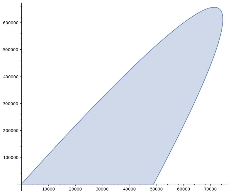
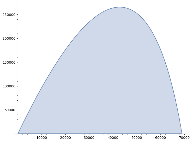
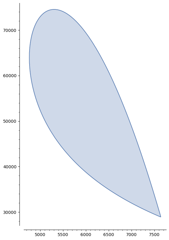
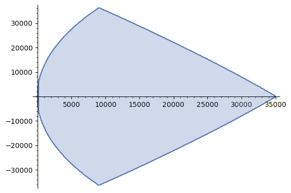
In Figure 2 we present three examples of Hurwitz slices for $n=5$. The multiplicity of any polynomial on the upper arc in (A) is $(3,0,(1))$ at all points but the two endpoints. At the left endpoint the multiplicity is $(3,0,(1))$ with a double root at $0$ and $(2,1,(1))$ at the right endpoint with a root at $\approx\pm 21i$. The bottom line corresponds to the multiplicity $(4,1,(0))$. The same multiplicities are true for the arcs in (B). In (C) any boundary point has multiplicity structure $(5,0,(0))$.

In general, in a Hurwitz slice not every multiplicity occurs. It is an open question to classify which multiplicities do occur in Hurwitz slices. Is a Hurwitz slice where the first coefficients are fixed always connected? We do not expect connectivity for other slices. By Theorem 3.3 for $k<\frac{n}{3}$ the Hurwitz slice can at least not be strictly convex. Adm, Garloff and Tyaglov classified [1, Thm. 4.9] the subset of weakly Hurwitz polynomials with $r$ roots in the interior of the left half-plane. They showed that a monic polynomial $f(T)=p_{0}(T^{2})+Tp_{1}(T^{2})\in\mathbb{R}[T]$ is weakly Hurwitz with $r$ roots in the open left half-plane if and only if the first $r$ principal minors of the finite Hurwitz matrix are negative and the remaining ones are $0$ and if the polynomial $\operatorname{gcd}(p_{0},p_{1})$ has only negative roots. Do the roots of $\operatorname{gcd}(p_{0},p_{1})$ correspond to the root multiplicity $(s,\mu)$? Finally, one could study the combinatorics and geometry of general stable slices.

4. A Grace-Walsh-Szegő like theorem for symmetric polynomials in few multiaffine polynomials

Throughout this section, let $\mathbb{H}$ be a closed half-plane and let $\underline{X}=(X_{1},\ldots,X_{n})$ be a tuple of $n$ variables.

The main result of this section is a generalization of the well-known Grace-Walsh-Szegő coincidence theorem and a generalization of the degree principle in Theorem 4.6, Corollary 4.11 and Corollary 4.8. We refer to [19, p. 107] for background on the coincidence theorem. The main tool in this section will be our results on root multiplicities of local extreme points of stable slices from Section 2.

Theorem 4.1 (Grace-Walsh-Szegő coincidence theorem).

Let $\mathcal{A}$ be a closed circular region and let $f\in\mathbb{C}[\underline{X}]$ be a multiaffine symmetric polynomial. If $\deg(f)=n$ or if $\mathcal{A}$ is convex, then for any $(x_{1},\ldots,x_{n})\in\mathcal{A}^{n}$ there exists a $y\in\mathcal{A}$ with $f(x_{1},\ldots,x_{n})=f(y,\ldots,y)$.

We address a generalization to the case where the symmetric polynomial $f$ is no longer assumed to be multiaffine but can be written as a polynomial in $k$ multiaffine symmetric polynomials. However, we cannot expect a diagonal point in $\mathcal{A}$ any longer.

Definition 4.2.

Let $V\subseteq\mathbb{C}^{n}$ be a variety. We say $V$ is $\mathbb{H}$-stable if $V\cap\mathbb{H}^{n}=\emptyset$. Moreover, we say a polynomial $f\in\mathbb{C}[\underline{X}]$ is $\mathbb{H}$-stable if the variety $V(f)$ is $\mathbb{H}$-stable.

Remark 4.3.

In Definition 4.2 we follow the standard terminology for stability of multivariate polynomials which is in contrast to the definition of stability of univariate polynomials in Definition 2.1. We say that a multivariate polynomial is $\mathbb{H}$-stable if there is no zero in $\mathbb{H}^{n}$, while any root of a univariate polynomial has to be contained in $\mathbb{H}$ if it is $\mathbb{H}$-stable. Since the complement of $\mathbb{H}$ is an open half-plane $\mathbb{H}^{c}$ one can see that for univariate polynomials $\mathbb{H}$-stability in Definition 2.1 is the same as $\mathbb{H}^{c}$-stability in Definition 4.2.

Recall that any $n$-variate symmetric polynomial can uniquely be written as a polynomial in the first $n$ elementary symmetric polynomials by the fundamental theorem of symmetric polynomials. We are interested in symmetric polynomials, which can be written as polynomials in few linear combinations of elementary symmetric polynomials, which generalizes the notion of multiaffine symmetric polynomials.

Definition 4.4.

Let $f\in\mathbb{C}[\underline{X}]$ be a symmetric polynomial and write $f$ in terms of elementary symmetric polynomials, say $f=g(e_{1},\dots,e_{n})$.

1. We say that $f$ is $(l_{1},\dots,l_{k})$-sufficient if $g\in\mathbb{C}[l_{1},\dots,l_{k}]$ where $l_{1},\dots,l_{k}$ are linear forms.

2. Moreover, we say that a symmetric variety $V\subseteq\mathbb{C}^{n}$ is $(l_{1},\dots,l_{k})$-sufficient, if it can be described by $(l_{1},\dots,l_{k})$-sufficient polynomials.

Remark 4.5.

A polynomial $f$ is $(l_{1},\dots,l_{k})$-sufficient for some linear forms $l_{1},\dots,l_{k}$, if and only if $f$ can be written as a polynomial in $k$ symmetric and multiaffine polynomials. In particular, every symmetric and multiaffine polynomial is $l_{1}$-sufficient for some linear form $l_{1}$.

For instance, the polynomial $e_{1}^{2}+e_{2}+2e_{3}$ is $(l_{1},l_{2})$ sufficient for $l_{1}(y)=y_{1}$ and $l_{2}(y)=y_{2}+2y_{3}$. For checking sufficiency of polynomials and more on the notion of sufficiency we refer to Subsection 3.3 in [21].

The following Theorem is our main result of this section and can be seen at the same time as some kind of degree principle for checking stability and as some kind of generalization of Grace-Walsh-Szegő’s coincidence theorem.

Theorem 4.6.

Let $V\subseteq\mathbb{C}^{n}$ be a symmetric $(l_{1},\dots,l_{k})$-sufficient variety. Then $V$ is $\mathbb{H}$-stable, if and only if $V\cap\mathbb{H}_{2(k+2),k+2}=\emptyset.$

Proof.

The forward implication follows from the definition. To prove the converse implication we suppose that $V$ is not $\mathbb{H}$-stable and we want to show that

$$V\cap\mathbb{H}_{2(k+2),k+2}\neq\emptyset.$$

So let $x\in V\cap\mathbb{H}^{n}$ and consider $z:=(e_{1}(x),\dots,e_{n}(x))\in\mathcal{S}_{\mathbb{H}}\cap L^{-1}(a)$, where

$$\begin{array}[]{rcccc}L&:&\mathbb{C}^{n}&\,\,\longrightarrow&\mathbb{C}^{k}\\[2.15277pt] &&y&\longmapsto&(l_{1}(y),\dots,l_{k}(y))\end{array}\quad\text{and}\quad a:=L\left(z\right)\in\mathbb{C}^{k}.$$

Then by Corollary 2.10 we find $\tilde{z}\in\mathcal{S}^{2(k+2),k+2}_{\mathbb{H}}\cap L^{-1}(a)$, i.e. there is $\tilde{x}\in\mathbb{H}_{2(k+2),k+2}$ with $\tilde{z}=(e_{1}(\tilde{x}),\dots,e_{n}(\tilde{x}))$ and $L(\tilde{z})=a=L(z)$. This means that $\tilde{x}\in V$, since $V$ is $(l_{1},\dots,l_{k})$-sufficient. ∎

The following proposition is a direct consequence of the unique representation of a symmetric polynomial of degree $d$ in terms of the elementary symmetric polynomials and may serve as a motivation for Definition 4.4. We consider new variables $\underline{Z}=(Z_{1},\ldots,Z_{n})$. For a symmetric polynomial in $\mathbb{R}[\underline{X}]$ there is a unique polynomial $g\in\mathbb{R}[\underline{Z}]$ with $f(\underline{X})=g(e_{1}(\underline{X}),\ldots,e_{n}(\underline{X}))$.

Proposition 4.7.

Let $f\in\mathbb{R}[\underline{X}]$ be a symmetric polynomial of degree $d$. Then $f$ is $\left(Z_{1},\dots,Z_{d}\right)$-sufficient, i.e. $f$ can be written as $f=g(e_{1},\dots,e_{d})$ for some $g\in\mathbb{C}[Z_{1},\dots,Z_{d}]$. Moreover, $g$ is linear in $Z_{\lfloor\frac{d}{2}\rfloor+1},\dots,Z_{d}$.

Proof.

See Proposition 2.3 in [20]. ∎

From Theorem 4.6 and Proposition 4.7, we obtain immediately the following double-degree principle.

Corollary 4.8 (Double-degree principle).

Let $f_{1},\dots,f_{m}\in\mathbb{C}[\underline{X}]$ be symmetric polynomials of degree at most $d$. Then

$$V(f_{1},\dots,f_{m})\cap\mathbb{H}^{n}=\emptyset\iff V(f_{1},\dots,f_{m})\cap\mathbb{H}_{2(d+2),d+2}=\emptyset.$$

Remark 4.9.

In the case that $\mathbb{H}$ is a rotation of the upper half-plane we can replace $\mathbb{H}_{2(d+2),d+2}$ by $\mathbb{H}_{d,d}$ in Corollary 4.8. This follows immediately from Remark 2.11 for $d=2$ and the case $d=1$ is trivial.

Although one might hope for a stronger degree principle, the next example shows that stability of a variety defined by symmetric polynomials of degree $\leqslant d$ cannot always be checked by testing points with at most $d$ many distinct coordinates.

Example 4.10.

Let $n=4$ and consider $f_{1}:=e_{1}-23i$, $f_{2}:=e_{2}-463i$ and $f_{3}:=e_{3}-8461i$. Then

$$V(f_{1},f_{2},f_{3})\cap\mathbb{H}_{+}^{4}\neq\emptyset\leavevmode\nobreak\ \text{and}\leavevmode\nobreak\ V(f_{1},f_{2},f_{3})\cap\{x\in\mathbb{H}_{+}^{4}\leavevmode\nobreak\ |\leavevmode\nobreak\ |\{x_{1},\dots,x_{4}\}|\leqslant 3\}=\emptyset,$$

which can either be computed directly using Gröbner basis or concluded by using Example 2.12.

From Remark 4.5 and Theorem 4.6, we get immediately the following generalization of Grace-Walsh-Szegő’s coincidence Theorem.

Corollary 4.11.

Let $f\in\mathbb{C}[\underline{X}]$ be a symmetric polynomial that can be written as a polynomial in $k$ symmetric and multiaffine polynomials. Furthermore, let $x\in\mathbb{H}^{n}$. Then there is $\tilde{x}\in\mathbb{H}_{2(k+2),k+2}$ with $f(x)=f(\tilde{x}).$

Note that different from Grace-Walsh-Szegő’s coincidence theorem we do not require $f$ to be multiaffine. But our result is weaker in the following sense: We do not consider closed inner or outer circle. Moreover, if $f$ is symmetric of degree $d\geq 2$ and multiaffine and $x\in\mathcal{A}^{n}$, then we can find $\tilde{x}\in\mathbb{H}_{d,d}^{n}$ with

$$f(x)=f(\tilde{x}),$$

while one can find $y\in\mathbb{H}$ with Grace-Walsh-Szegő’s coincidence Theorem such that

$$f(x)=f(y,\ldots,y).$$

Remark 4.12.

The results of this section translate to open half-planes in the following way: Let $\mathbb{G}$ be an open circular region and $x\in\mathbb{G}^{n}$. Then $x\in\mathbb{H}^{n}$ for some closed half-plane $\mathbb{H}\subset\mathbb{G}$. So $\mathbb{G}_{2(k+2),k+2}$ can be replaced by $\mathbb{G}_{0,3(k+2)}$ in Theorem 4.6 and Corollary 4.11 and $\mathbb{G}_{2(d+2),d+2}$ can be replaced by $\mathbb{G}_{0,3(d+2)}$ in Corollary 4.8.

If $\mathbb{H}=\mathbb{H}_{+}$ is the upper half-plane, one can also formulate a generalization of the half-degree principle.

Theorem 4.13 (Half-degree principle for the upper half-plane).

Let $f\in\mathbb{C}[\underline{X}]$ be a symmetric polynomial of degree $d\leqslant n$ and $\lambda,\mu\in\mathbb{R}$. Then

$$\inf_{x\in\mathbb{H}_{+}^{n}}\lambda\operatorname{Re}(f(x))+\mu\operatorname{Im}(f(x))=\inf_{x\in{\mathbb{H}_{+}}_{k,k}}\lambda\operatorname{Re}(f(x))+\mu\operatorname{Im}(f(x)),$$

where $k=\max\{\lfloor\frac{d}{2}\rfloor,2\}$.

Proof.

Write $f=g(e_{1},\dots,e_{d})$ for some $g\in\mathbb{R}[Z_{1},\dots,Z_{d}]$ and note that $g$ is linear in $Z_{\lfloor\frac{d}{2}\rfloor+1},\dots,Z_{d}$ by Proposition 4.7. Let now $x\in\mathbb{H}_{+}^{n}$ and consider $z:=(e_{1}(x),\dots,e_{n}(x))\in\mathcal{S}(a)$, where $a:=(e_{1}(x),\dots,e_{k}(x))$. Since $\mathcal{S}(a)$ is compact and $g$ is linear on $\mathcal{S}(a)$, the minimum of $g$ on $\mathcal{S}(a)$ is taken on an extreme point of the convex hull of $\mathcal{S}(a)$, i.e. on a point $\tilde{z}\in\mathcal{S}^{k,k}$ by Remark 2.11. ∎

5. Conclusion and open questions

In our paper, we restrict to half-plane stable polynomials. However, the notion of stable polynomials can be formulated for any circular region, i.e. any open or closed subset of $\mathbb{C}$ that is bounded by a circle or by a line. It is well known that a Möbius transformation maps circular regions to circular regions and testing stability of a polynomial can always be reduced to testing whether an associated polynomial of possibly smaller degree is $\mathbb{H}_{+}$-stable. Let $\mathcal{A}$ be a circular region and let $\phi(z)=\frac{az+b}{cz+d}$ be a Möbius transformation mapping $\mathbb{H}_{+}$ to $\mathcal{A}$. Then a monic polynomial $f\in\mathbb{C}[T]$ is $\mathcal{A}$-stable if and only if the polynomial $(cT+d)^{\deg(f)}f\left(\frac{aT+b}{cT+d}\right)$ is $\mathbb{H}_{+}$-stable. The roots of the associated polynomial are contained in the image of the roots of $f$ under $\phi^{-1}$. However, the obtained polynomial must not necessarily be monic or can have fewer roots. This happens if one of the roots is a pole point of $\phi^{-1}$. For instance, if $f=p\cdot(T-1)$ is $\{x\in\mathbb{C}:|x|\leqslant 1\}$-stable and $p$ has only roots different from $1$, then

$$(T+i)^{\deg{(p)}}p\left(\frac{T-i}{T+i}\right)(T+i)\left(\frac{T-i}{T+i}-1\right)=(T+i)^{\deg{(p)}}p\left(\frac{T-i}{T+i}\right)\cdot(-2i)$$

is a non-monic $\mathbb{H}_{+}$-stable polynomial of degree $\deg(f)-1$. Thus our proofs of Theorems 2.4 and 4.6 do not transfer to circular regions which are bounded by a circle. Nevertheless, the following question seems worth to be asked.

Question 5.1.

Can Theorem 2.4 and Theorem 4.6 be adapted to arbitrary circular regions? If not, can our generalization of the coincidence theorem be extended to a closed domain bounded by a circle?

Question 5.2.

Can our double-degree principle in Corollary 4.8 be improved?

Finally, we gave a possible combinatorial encoding for subsets of the set of weakly Hurwitz polynomials. For hyperbolic polynomials, there is the rich interplay between geometry and combinatorics of its roots. Hyperbolic slices with fixed first $k$ coefficients and their strata are known to be contractible. Moreover, Lien [15] showed that in this case, one can reconstruct the compositions of the stratification from the compositions of its $0$-dimensional strata, and Schabert and Lien [16] showed that this poset has a structure similar to polytopes, giving the same bounds on its number of $i$-dimensional strata. We ask if similar results hold for Hurwitz slices with fixed first $k$ coefficients.

References

• [1] M. Adm, J. Garloff, and M. Tyaglov. Total nonnegativity of finite Hurwitz matrices and root location of polynomials. J. Math. Anal. Appl., 467(1):148–170, 2018.
• [2] V. I. Arnold. Hyperbolic polynomials and Vandermonde mappings. Funktsional. Anal. i Prilozhen., 20(2):52–53, 1986.
• [3] B. A. Asner, Jr. On the total nonnegativity of the Hurwitz matrix. SIAM J. Appl. Math., 18:407–414, 1970.
• [4] P. Brändén. Polynomials with the half-plane property and matroid theory. Advances in Mathematics, 216(1):302–320, 2007.
• [5] P. Brändén and D. G. Wagner. A converse to the Grace-Walsh-Szegő theorem. Math. Proc. Cambridge Philos. Soc., 147(2):447–453, 2009.
• [6] M.-J. Ding and B.-X. Zhu. Stability of combinatorial polynomials and its applications. arXiv preprint arXiv:2106.12176, 2021.
• [7] S. Engelberg. Mathematical Introduction To Control Theory, A, volume 4. World Scientific Publishing Company, 2015.
• [8] S. Fisk. Polynomials, roots, and interlacing–version 2. arXiv preprint math/0612833, 2008.
• [9] A. B. Givental. Moments of random variables and the equivariant Morse lemma. Uspekhi Mat. Nauk, 42(2(254)):221–222, 1987.
• [10] G. Harris and C. Martin. The roots of a polynomial vary continuously as a function of the coefficients. Proc. Amer. Math. Soc., 100(2):390–392, 1987.
• [11] O. J. Heilmann and E. H. Lieb. Theory of monomer-dimer systems. Communications in mathematical Physics, 25(3):190–232, 1972.
• [12] A. Hurwitz. Über die Bedingungen, unter welchen eine Gleichung nur Wurzeln mit negativen reellen Teilen besitzt. Mathematische Annalen, Bd. 46:273–284, 1895.
• [13] J. H. B. Kemperman. A Hurwitz matrix is totally positive. SIAM J. Math. Anal., 13(2):331–341, 1982.
• [14] V. P. Kostov. On the geometric properties of Vandermonde’s mapping and on the problem of moments. Proc. Roy. Soc. Edinburgh Sect. A, 112(3-4):203–211, 1989.
• [15] A. Lien. Hyperbolic polynomials and starved polytopes. arXiv preprint arXiv:2307.03239, 2023.
• [16] A. Lien and R. Schabert. Shellable slices of hyperbolic polynomials and the degree principle. in preperation.
• [17] J. C. Maxwell. On governors. Proceedings of the Royal Society of London, (16):270–283, 1868.
• [18] I. Meguerditchian. A theorem on the escape from the space of hyperbolic polynomials. Math. Z., 211(3):449–460, 1992.
• [19] Q. I. Rahman and G. Schmeisser. Analytic theory of polynomials, volume 26 of Lond. Math. Soc. Monogr., New Ser. Oxford: Oxford University Press, 2002.
• [20] C. Riener. On the degree and half-degree principle for symmetric polynomials. Journal of Pure and Applied Algebra, 216(4):850–856, 2012.
• [21] C. Riener and R. Schabert. Linear slices of hyperbolic polynomials and positivity of symmetric polynomial functions. J. Pure Appl. Algebra, 228(5):Paper No. 107552, 21, 2024.