Large Language Model Meets Graph Neural Network in Knowledge Distillation

Abstract.

Despite recent community revelations about the advancements and potential applications of Large Language Models (LLMs) in understanding Text-Attributed Graph (TAG), the deployment of LLMs for production is hindered by its high computational and storage requirements, as well as long latencies during model inference. Simultaneously, although traditional Graph Neural Networks (GNNs) are light weight and adept at learning structural features of graphs, their ability to grasp the complex semantics in TAG is somewhat constrained for real applications. To address these limitations, we concentrate on the downstream task of node classification in TAG and propose a novel graph knowledge distillation framework, termed Linguistic Graph Knowledge Distillation (LinguGKD), using LLMs as teacher models and GNNs as student models for knowledge distillation. It involves TAG-oriented instruction tuning of LLM on designed tailored prompts, followed by propagating knowledge and aligning the hierarchically learned node features from the teacher LLM to the student GNN in latent space, employing a layer-adaptive contrastive learning strategy. Through extensive experiments on a variety of LLM and GNN models and multiple benchmark datasets, the proposed LinguGKD significantly boosts the student GNN’s predictive accuracy and convergence rate, without the need of extra data or model parameters. Compared to teacher LLM, distilled GNN achieves superior inference speed equipped with much fewer computing and storage demands, when surpassing the teacher LLM’s classification accuracy on some of benchmark datasets.

1. Introduction

Text-Attributed Graphs (TAGs) are extensively utilized across diverse domains, ranging from social network analysis (Li et al., 2022) to bioinformatics (Yang and Shi, 2023). While traditional Graph Neural Networks (GNNs) excel at interpreting graph structures, they often struggle with semantic processing (Li et al., 2023). The advent of Large Language Models (LLMs), exemplified by ChatGPT (Ouyang et al., 2022) and Llama (Touvron et al., 2023), is revolutionizing this field. These models, distinguished by their contextual and relational understanding, offer a novel perspective in evaluating TAGs, which typically integrate structured and unstructured data. There has been a concerted effort within the community to amalgamate LLMs with GNNs, employing fine-tuning technologies for graph inference tasks (Wei et al., 2024; Wang et al., 2024; Fatemi et al., 2023; Ye et al., 2024). This approach has yielded promising initial results, revealing the capabilities of LLMs in understanding graph structures. Such a collaborative approach not only amplifies the semantic interpretation in TAGs but also lays the groundwork for more profound exploration in graph learning. It demonstrates the immense potential of harmonizing LLMs, GNNs, and instruction tuning in a variety of graph learning applications.

Recent advancements in LLMs-based graph learning have explored diverse approaches for improving graph reasoning (Li et al., 2024). These methods range from employing LLMs for feature extraction to enhance GNN performance (He et al., 2023; Chen et al., 2024; Wei et al., 2024), to utilizing LLMs in graph structure generation or optimization (Wang et al., 2024; Fatemi et al., 2023; Ye et al., 2024). This integration leverages LLMs’ ability to interpret complex graph structures and semantic nuances, demonstrating synergistic gains. However, the practical application of LLMs in graph data processing faces significant challenges, particularly due to their large parameter sizes, often exceeding billions (Hugging Face, 2024). This leads to high computational and storage demands, making cost-effective and widespread deployment challenging. Additionally, LLMs’ extended latency during inference presents practical limitations in operational settings. Addressing these challenges, a key research focus is to develop advanced techniques for compressing LLMs while maintaining their graph reasoning abilities. Knowledge distillation stands out as a promising strategy, enabling the transfer of LLM insights to more compact GNNs. The idea not only aims to reduce model size and computational demands of LLM but also capitalizes on GNNs’ strengths in processing structural data. By integrating the semantic understanding of LLMs with the structural mining of GNNs, it is expected to optimize graph reasoning tasks, facilitating more effective and adaptable real-world applications.

Under the above motivation, we explore the innovative integration of graph knowledge distillation from complex LLMs as teachers to lightweight GNNs as students, with a focus on node classification tasks. Acknowledging the inherent architectural differences and the distinct vector spaces of LLMs and GNNs, we introduce a novel framework-Linguistic Graph Knowledge Distillation (LinguGKD). It begins by instruction tuning a pre-trained LLM (PLM) with carefully designed node classification instruction prompts. It then employs a layer-adaptive contrastive distillation strategy, complemented by a feature alignment mechanism to synchronize LLM and GNN feature spaces, transferring hierarchical node features from LLM to GNN. By doing so, it can propagate the teacher LLM’s deep semantic knowledge and intricate understanding of graph structures to the student GNN, leading to better performance of node classification in TAG.

Our extensive experimental evaluations, spanning various LLM and GNN architectures, and multiple benchmark datasets, demonstrate the proposed LinguGKD’s effectiveness in distilling the graph knowledge from teacher LLMs to student GNNs. More specifically, the distilled GNNs exhibit a significant reduction in model complexity for real application, with only a fractional parameter count compared to LLMs and a notable increase in model inference speed. Impressively, this efficiency is achieved with minimal performance trade-offs. From the perspective of effectiveness, the distilled GNNs show improved node classification accuracy and quicker convergence without requiring additional data or architectural modifications. These results not only validate our framework’s classification performance in TAG but also highlight its potential in enhancing the practicality of LLMs for graph data processing, striking for an optimal balance between effectiveness and efficiency.

The principal contributions of this paper are summarized as follows:

• We conceptualize node classification in TAG and fine-tune pre-trained LLMs with designed tailored instruction prompts, which is called LinguGraph LLM. It effectively enhances LLMs’ classification accuracy on benchmark datasets, although it consumes heavy computing resources and storage space deployed on devices with long latency of model inference.

• To moderate the efficiency of LLMs, we introduce LinguGKD, an innovative TAG-oriented graph knowledge distillation framework, leveraging the tuned LinguGraph LLM as a sophisticated teacher model. Here, a contrastive layer-adaptive distillation mechanism is proposed to capture and transfer the LLM’s profound semantic and structural knowledge to a streamlined student GNN.

• Extensive experimental evaluations across diverse LLM and GNN models as well as multiple benchmark datasets validate LinguGKD’s performance on improving both node classification effectiveness and model inference efficiency, while the distilled GNNs can be swiftly deployed on users’ terminal devices for potentially real application scenarios.

The remainder of this paper is organized as follows: Section 2 formally defines the research problem; Section 3 delves into the details of the LinguGKD framework; Section 4 presents our extensive experimental results and analysis; Section 5 reviews relevant literature; and Section 6 concludes the paper, suggesting directions for future research.

2. Preliminaries

Definition 0 (Text-Attributed Graph).

A Text-Attributed Graph (TAG) is a graph where each node is associated with textual data. Formally, a TAG is denoted as $\mathcal{G}=(\mathcal{V},\mathcal{E},\mathcal{X})$, where $\mathcal{V}=\{v_{i}\}_{i=1}^{n}$ represents the set of nodes, with $n$ being the total node count, $\mathcal{E}$ is the set of edges with $e_{ij}\in\mathcal{E}$ indicating an edge between nodes $v_{i}$ and $v_{j}$, and $\mathcal{X}=\{x_{i}\}_{i=1}^{n}$ denotes the node attributes, where $x_{i}$ represents the textual attribute of node $v_{i}$.

Given a TAG $\mathcal{G}$, GNNs are essential for interpreting the graph topological dependence:

Definition 0 (Graph Neural Network).

Graph Neural Networks (GNNs) are specialized for handling graph-structured data, primarily through a $k$-layer message-passing mechanism (Kipf and Welling, 2017), enabling the capture and analysis of $k$-hop node relationships and graph dynamics. This process is defined as:

(1) $$\textbf{h}_{v}^{(k)}=f(\textbf{h}_{v}^{(k-1)},\oplus_{u\in\mathcal{N}(v)}g(\textbf{h}_{u}^{(k-1)},\textbf{h}_{v}^{(k-1)}))$$

where $\textbf{h}_{v}^{(k)}$ is the feature representation of node $v$ at the $k$-th layer, $\mathcal{N}(v)$ includes $v$’s neighboring nodes, and functions $g(\cdot)$ and $f(\cdot)$ are trainable and responsible for aggregating neighbor features and updating node features, respectively. The operator $\oplus$ denotes an aggregation function, such as summation (Zhang, 2020) or averaging (Kipf and Welling, 2017).

While GNNs excel at processing graph structures, they have limitations in understanding individual node semantics. Taking advantage of the capability of LLM’s semantic feature learning, LLM-based Graph Knowledge Distillation can be designed by distilling knowledge from a teacher LLM to a student GNN, enhancing the GNN’s capability in interpreting node semantics and complex graph topology. It can be defined as follows:

Definition 0 (LLM-based Graph Knowledge Distillation).

An LLM-based Graph Knowledge Distillation (GKD) framework can be formulated as a quintuple: ¡$\mathcal{M}_{T}$, $\mathcal{M}_{S}$, $\mathcal{S}$, $\mathcal{F}$, $\mathcal{A}$¿, where teacher model $\mathcal{M}_{T}$ is a Transformer (Vaswani et al., 2017) based LLM, fine-tuned on TAG $\mathcal{G}$ for generative graph inference tasks; $\mathcal{M}_{S}$ denotes the student GNN specified for discriminative tasks; $\mathcal{F}$ represents the knowledge to be transferred from $\mathcal{M}_{T}$ to $\mathcal{M}_{S}$ via distillation scheme $\mathcal{S}$, learned by extraction algorithm $\mathcal{A}$. The distillation process can be formulated as follows:

(2) $$\mathcal{F}=\{\mathcal{F}_{T},\mathcal{F}_{S}\}=\{\mathcal{A}_{T}(\mathcal{M}_{T},\mathcal{G}),\mathcal{A}_{S}(\mathcal{M}_{S},\mathcal{G})\}$$

(3) $$\mathcal{L}_{D}=loss(\mathcal{F}_{S},\mathcal{F}_{T})$$

(4) $$\mathcal{M}_{S}^{new}=\mathcal{S}(\mathcal{M}_{S},\mathcal{L}_{d})$$

where $\mathcal{A}_{T}$ and $\mathcal{A}_{S}$ are knowledge extraction algorithms of $\mathcal{M}_{T}$ and $\mathcal{M}_{S}$, respectively; $loss(\cdot)$ denotes the divergence function (e.g., Kullback-Leibler divergence), $\mathcal{M}_{S}^{new}$ is the distilled student model that we actually required.

3. Approach

Figure 1. The overall TAG-oriented graph knowledge distillation framework of LinguGKD.

Figure 1 showcases the LinguGKD framework for TAG-oriented graph knowledge distillation, highlighting three key components: teacher feature learning by the LLM, student feature learning by the GNN, and layer-adaptive contrastive distillation loss between the two feature sets. Prior to detailing these crucial modules, we elaborate how to fine-tune a TAG-oriented pre-trained LLM to generate node categories by our designed tailored instruction prompts.

3.1. TAG Instruction Tuning of Pre-trained LLM

Given a TAG $\mathcal{G}=(\mathcal{V},\mathcal{E},\mathcal{X})$, a center node $v_{i}$ and a specific neighbor hop $k$, we can obtain a collection of neighbor subgraphs from structural-free up to $k$-th hop: $\mathcal{G}_{i}^{k}=\{\mathcal{G}_{i}^{(l)}\}_{l=0}^{k}$, where $\mathcal{G}_{i}^{(k)}=(v_{i},\mathcal{N}_{i}^{(k)},\mathcal{E}_{\mathcal{N}_{i}^{(k)}},\mathcal{X}_{\mathcal{N}_{i}^{(k)}})$ denotes the $k$-th hop subgraphs, in which $\mathcal{E}_{\mathcal{N}_{i}^{(k)}}$ is the $k$-hop neighbors of $v_{i}$, $\mathcal{E}_{\mathcal{N}_{i}^{(k)}},\mathcal{X}_{\mathcal{N}_{i}^{(k)}}$ are the corresponding edges and textual node attributes within the subgraph, respectively.

To enable the PLM to accurately perform node classification tasks, it’s essential to craft comprehensive and clear instruction prompts. For a given $\mathcal{G}_{i}^{(k)}$, drawing on (Ye et al., 2024), we define the specific for an instruction prompt $\textbf{p}_{k}$, which consists of three components: task-specific instructions $\mathcal{I}$ that delineate the expected model action, the structural prompt $\tau_{k}$ that is the natural language description of the subgraph, and a task-relevant query $\mathcal{Q}$, typically presented as a detailed question. The construction of $\textbf{p}_{k}$ is a concatenation of these elements, as shown in the lower left part of Figure 1:

(5) $$\textbf{p}_{k}=concat(\mathcal{I},\tau_{k},\mathcal{Q})$$

In alignment with OpenAI’s Prompt Engineering principles (OpenAI, 2023), we carefully design $\mathcal{I}$ and $\mathcal{Q}$ to each classification task as follows:

Prompt 1 (TAG Node Classification Instruction).

Implement a node classification system for {{type of network}}, representing nodes as tuples (node_{id},{degree},{attribute}). Classify nodes into [{{list of classification categories}}] based on attributes and link relations. {{classification criteria}}. Consider degree for influence and network position, title keywords for research areas, and citation links for thematic connections. When unclear, classify based on the majority theme of linked nodes.

Prompt 2 (TAG Node Classification Query).

Which category should (node_{{id}},{{node degree}},{{node attributes}}) be classified as?

In these templates, each node is represented by a tuple that encapsulates the node’s id, degree and the corresponding textual attributes. The placeholders within curly braces {{}} are filled based on the specific graph data. More precisely, the term {{type of network}} specifies the network’s architecture, while {{list of classification categories}} enumerates the potential categories for node classification. Furthermore, {{classification criteria}} denotes the optional prior knowledge that assist the LLM in the precise generation of labels for the center node.

In crafting the structural prompt, we prioritize key elements such as node textual attributes, multi-order neighbor interactions, node degrees, and inter-node connections, aligned with conventional multi-layer message-passing GNNs’ principles. Referring to the strategies from (Ye et al., 2024), we develop a linguistic structural encoder $f_{e}$ that transforms $\mathcal{G}_{i}^{(k)}$ into the detailed natural language description, represented as $\tau_{k}$:

(6) $$\tau_{k}=f_{e}(\mathcal{G}_{i}^{(k)})$$

The prompt template of $f_{e}$ is meticulously designed as follows:

Prompt 3 (TAG Structural Prompt).

(node_{id}, {{node degree}}, {{node attributes}}) is connected within k hops to {{k-th hop neighbors}} through paths that may involve {{intermediate paths}}.

In this context, {{k-th hop neighbors}} refers to the ensemble of neighbors reachable at $k$-th hop in $\mathcal{N}_{i}^{(k)}$. Each neighbor in this list is characterized by a tuple that encapsulates its id, degree, and attributes, mirroring the representation of the central node. Furthermore, {{intermediate paths}} represents the sequences of paths connecting the central node $v_{i}$ to its $k$-th hop neighbors, encompassing the edges defined within $\mathcal{E}_{\mathcal{N}_{i}^{(k)}}$. This template meticulously outlining the connectivity and relational dynamics within the subgraph based on node degrees, attributes, and the specified hop distances.

Iterating the structural encoding process, we can methodically generate a structural prompt for every subgraph within $\mathcal{G}_{i}^{k}$, leading to the the assembly of the $k$-hop structural prompt set $\mathcal{T}=\{f_{e}(\mathcal{G}_{i}^{(l)})\}_{l=0}^{k}$ for the central node $v_{i}$. Notably, $l=0$ concentrating on $v_{i}$’s textual attributes exclusively. This iterative generation of structural prompts systematically captures the nuanced relational dynamics at varying degrees of connectivity, from the immediate vicinity ($l=0$) extending to the broader $k$-hop network. By concatenating instruction $\mathcal{I}$ and query $\mathcal{Q}$ with various structural prompts, we can obtain a set of graph instruction prompts $\mathcal{P}$:

(7) $$\mathcal{P}=\{concat(\mathcal{I},\tau_{l},\mathcal{Q})\}\quad\forall\tau_{l}\in\mathcal{T}$$

Then we adopt instruction tuning (Zhang et al., 2023; Si et al., 2023; Honovich et al., 2022) to specifically tailor PLMs for generative node classification tasks. Specifically, each prompt $\textbf{p}_{l}\in\mathcal{P}$ is utilized to directly fine-tune the PLM to strictly generate the semantic category $\textbf{y}_{i}$ for the corresponding center node, without any modification of the pre-trained tokenizer and vocabulary. We utilize negative log-likelihood loss as our objective function:

(8) $$\mathcal{L}_{T}(\mathcal{P})=-\sum_{\textbf{p}_{l}\in\mathcal{P}}\sum_{j=1}^{|\textbf{y}|}\log p(\hat{y}_{j}|\textbf{p}_{l},\hat{y}_{<j})$$

where $y_{j}$ refers to the $j$-th token that LLM generated for node label. Employing this instruction tuning methodology, we develop a highly proficient LLM adept in node classification. This fine-tuned LLM, we call it LinguGraph LLM, then acts as the teacher model $\mathcal{M}_{T}$ in the subsequent graph knowledge distillation process. For an in-depth exploration of the unique Instruction, Structural, and Query prompts, as well as a detailed walkthrough of generating node classification through the dynamic interaction with the LinguGraph LLM, please refer to Appendix A.

3.2. LinguGraph LLM-based Knowledge Distillation

Here, we detail the two key parts of the proposed LinguGKD framework, focusing on the challenge of transferring insights from complex teacher LLMs to simpler student GNNs. It emphasizes aligning the node latent features extracted by both the LLM and the GNN within a unified latent space. In the following, we elaborate three pivotal phases of LinguGKD’s knowledge distillation process: extracting semantically-enhanced node features via LLMs; leveraging GNNs for structural node feature extraction; and implementing layer-adaptive alignment of semantic and structural features.

3.2.1. Teacher Feature Learning via LinguGraph LLM

We initially focus on leveraging the fine-tuned LinguGraph LLM $\mathcal{M}_{T}$ to extract semantically-enriched node features, encapsulating textual attributes and multi-order neighbor information, as shown in the Teacher Feature Learning module in Figure 1.

Building upon insights from (Xiao et al., 2023), we observe that tailored instructions significantly enhance the LLM’s proficiency in generating semantic features. Consequently, we toward leveraging the entire instruction prompt $\mathcal{P}$ for the extraction of node semantical features, rather than limiting to the structural prompt $\mathcal{T}$. Specifically, given that LLMs primarily use the transformer architecture (Vaswani et al., 2017), comprising an embedding layer for token translation, $n$-layer transformer with multi-head self-attention for deriving word-level nonlinear interrelations, and an output layer for specific generative tasks. For an instruction prompt $\textbf{p}\in\mathcal{P}$, we consider the feature of the last token $\rho_{|\textbf{p}|}$ from the final transformer layer as the $l$-order node latent feature, since the last token’s feature encapsulates the aggregated contextual information of the entire instruction prompt. This feature extraction is defined as:

(9) $$E^{L}=\mathcal{M}_{e}^{T}(\{\rho_{i}\}_{i=1}^{|\textbf{p}|}|W_{e}^{T})$$

(10) $$H=\mathcal{M}_{tr}^{T}(E^{T}|W_{tr}^{T})$$

(11) $$\textbf{f}_{l}^{L}=H_{|\textbf{p}|,:}$$

where $\mathcal{M}_{e}^{T}$ and $\mathcal{M}_{tr}^{T}$ represent the embedding and transformer modules of $\mathcal{M}_{T}$, respectively, with $W_{e}^{T},W_{tr}^{T}$ being their parameters. $\textbf{f}_{l}^{L}\in\mathbb{R}^{d_{L}}$ is the $l$-order node feature from prompt p, which encompasses the semantic structural feature of the central node, integrating neighbor details and extensive node attribute data; $d_{L}$ denotes the dimension of node latent features extracted by teacher LLM.

For distilling hierarchical node features from the teacher LLM, we then process each $l$-th order feature, $\textbf{f}_{l}^{L}$, through a specialized hop-specific neural filter, $\mathcal{M}_{f}^{l}$, which is proficient in filtering pertinent layer knowledge. Subsequently, a cross-hop neural feature projector, $\mathcal{M}_{p}$, restructures these features to the distillation feature space. The filtering and mapping process can be described as:

(12) $$\mathcal{M}_{f}^{l}(\textbf{f}_{l}^{L})=\sigma(W_{l}\textbf{f}_{l}^{L}+b_{l})\quad 0\leq l\leq k$$

(13) $$\hat{\textbf{f}}_{l}^{L}=f_{norm}(\mathcal{M}_{f}^{l}(\textbf{f}_{l}^{L}))$$

(14) $$\textbf{f}_{l}^{T}=\mathcal{M}_{p}(\hat{\textbf{f}}_{l}^{L}|W_{p},b_{p}))=\sigma(W_{p}\hat{\textbf{f}}_{l}^{L}+b_{p})$$

where $\textbf{f}_{l}^{T}\in\mathbb{R}^{d_{k}}$ symbolizes the adapted $l$-order teacher knowledge, poised for subsequent distillation steps; $W_{l},b_{l},W_{p},b_{p}$ are the trainable parameters for $\mathcal{M}_{f}^{l}$ and $\mathcal{M}_{p}$, respectively; $\sigma$ denotes the non-linear activation function.

Applying this process across all subgraph orders up to the $k$-th, we obtain a set of hierarchical teacher node features $\mathcal{F}_{T}=\{\textbf{f}_{l}^{T}\}_{l=0}^{k}$, which is then utilized in the subsequent graph knowledge distillation, serving as the specific knowledge to be distilled from the teacher LLM to the student GNN.

3.2.2. Student Feature Learning via GNN

We then introduce leveraging the student GNN $\mathcal{M}_{S}$ to extract multi-hop node features, as shown in the Student Feature Learning module in Figure 1. Our chosen student model can be any off-the-shelf GNN. The GNN is adept at interpreting graph structures through its message-passing mechanism. This mechanism enables central nodes to assimilate features from $k$-hop neighbors, capturing local graph structure nuances. Although GNN models vary across graph topologies, their core principle remains consistent: a structured message-passing process involving message construction, aggregation, and node feature updating. These stages allow GNNs to effectively represent intricate graph structures.

For a given $k$-hop neighbor subgraph $\mathcal{G}_{i}^{(k)}$ of a central node $v_{i}$, the $k$-order message aggregation process in GNN unfolds as follows:

(15) $$\textbf{f}_{j}^{(0)}=\mathcal{M}_{\text{e}}^{S}(x_{j}),\quad\forall v_{j}\in v_{i}\cup\mathcal{N}_{i}^{(k)}$$

(16) $$\textbf{m}_{ij}^{(l)}=\mathcal{M}^{(l)}(\textbf{f}_{i}^{(l-1)},\textbf{f}_{j}^{(l-1)},e_{ij}|W_{\mathcal{M}}),\quad 0<l\leq k$$

(17) $$\textbf{a}_{i}^{(l)}=\mathcal{A}^{(l)}\left(\{\textbf{m}_{ij}^{(l)}\mid j\in\mathcal{N}(i)\},W_{\mathcal{A}}\right)$$

(18) $$\textbf{f}_{l}^{G}=\mathcal{U}^{(l)}(\textbf{f}_{i}^{(l-1)},\textbf{a}_{i}^{(l)}|W_{\mathcal{U}})$$

where $x_{j}\in\mathcal{X}_{\mathcal{N}_{i}^{(k)}}$ means the attribute of node $v_{j}$, $\mathcal{M}_{e}^{S}$ is the text embedding model of $\mathcal{M}_{S}$, like bag-of-words or TF-IDF, converting node textual attributes into low-dimensional vector space, establishing the initial feature vector $\textbf{f}_{j}^{(0)}$. The functions $\mathcal{M}^{(l)}$, $\mathcal{A}^{(l)}$, and $\mathcal{U}^{(l)}$ perform message construction, aggregation, and node feature updates, respectively, during $l$-order message passing. The parameters $W_{\mathcal{M}}$, $W_{\mathcal{A}}$, and $W_{\mathcal{U}}$ are the associated weights. The output of the $l$-th message passing layer $\textbf{f}_{l}\in\mathbb{R}^{d_{G}}$, represents the $l$-th order feature of the central node $v_{i}$, reflecting its $l$-order neighbor structure and attributes.

Subsequently, we synchronize the node features into the unified distillation vector space via a normalization layer:

(19) $$\textbf{f}_{l}^{S}=f_{norm}(\textbf{f}_{l}^{G})\quad 0\leq l\leq k$$

where $\textbf{f}_{l}^{S}\in\mathbb{R}^{d_{k}}$ denotes the student knowledge, and $f_{norm}$ is a normalization function, typically batch or layer normalization. Applying this process across all subgraph orders up to the $k$-th, we obtain a set of hierarchical student node features $\mathcal{F}_{S}=\{\textbf{f}_{l}^{S}\}_{l=0}^{k}$.

In the next phase, we focus on aligning the student GNN’s learned node features $\mathcal{F}_{S}$ with those $\mathcal{F}_{T}$ from the teacher LLM. This alignment ensures that the LLM’s rich semantic knowledge is effectively integrated into the GNN, enhancing its capability to process graph-structured data.

3.2.3. Layer-Adaptive Semantic-Structural Alignment

In graph inference, the relevance of node features varies with neighbor order: structural-free features highlight a node’s core attributes, lower-order features elucidate direct interactions, and higher-order features provide insight into distant connections, essential for understanding a node’s role in the network. To leverage the teacher LLM’s insights, we implement a Layer-Adaptive Semantic-Structural Alignment in LinguGKD framework, progressively syncing the teacher LLM’s node features with those of the student GNN across different neighbor orders.

To measure the divergence between layer-wise features of both models, we employ contrastive learning with the infoNCE loss, regulated by a temperature parameter $t$. It compares positive feature pairs (identical nodes learned by both teacher and student models) against negative pairs (LLM-learned features from nodes in different categories with the center node). The loss function for each $l$-order feature is expressed as:

(20) $$\mathcal{L}_{D}^{l}=-\mathbb{E}\left[\log\frac{\exp(sim(\textbf{f}_{l}^{S},\textbf{f}_{l}^{T})/t)}{\sum_{m=1}^{N}\exp(sim(\textbf{f}_{l}^{S},\textbf{f}_{l,(m)}^{T*})/t)}\right]$$

where $\textbf{f}_{l}^{T*}$ represents the $l$-th order feature of a node from the negative set, and $N$ means the number of negative samples.

Recognizing the unique importance of different-order neighbor structures in various downstream tasks, we introduce a trainable distillation factor $\gamma$ for each layer’s distillation loss. The cumulative layer-adaptive contrastive distillation loss is finally calculated as:

(21) $$\mathcal{L}_{\text{D}}=\sum_{l=0}^{k}\gamma_{l}\mathcal{L}_{\text{D}}^{l}$$

Here, each order’s distillation factor $\gamma_{l}$ ensures a balanced knowledge distillation, enabling the effective transfer of complex semantic and structural insights from the LLM to the GNN.

3.3. Model Training

In training the student GNN, acknowledging the different inference frameworks of the teacher and student models, it’s essential to not only distill knowledge from the teacher LLM but also to train a task-specific prediction layer for the GNN. Thus, we approach the student GNN’s training as a multi-task joint optimization challenge. For node classification tasks, we use a fully connected layer as the classifier:

(22) $$\hat{y}=\text{softmax}(W_{\text{G}}\textbf{f}_{k}^{S}+b_{\text{G}})$$

where $\textbf{f}_{k}^{S}$ denotes the output of $k$-th layer of GNN, $\hat{y}$ represents the predicted node label, with $W_{\text{G}}$ and $b_{\text{G}}$ being the weights and biases of the fully connected layer.

Subsequently, the node classification loss function, formulated as cross-entropy, is computed as:

(23) $$\mathcal{L}_{\text{G}}=-\sum_{c=1}^{C}y_{c}\log(\hat{y}_{c})$$

where $y_{c}$ denotes the one-hot encoding of the actual node label, and $\hat{y}_{c}$ is the predicted probability for each category. $C$ is the total number of nodes in the training set.

The overall training objective integrates the knowledge distillation loss $\mathcal{L}_{D}$ with the classification loss $\mathcal{L}_{G}$, obtaining a joint loss function:

(24) $$\mathcal{L}=\alpha\mathcal{L}_{G}+\beta\mathcal{L}_{D}$$

where $\alpha$ and $\beta$ are tunable factors, balancing the influence of both knowledge distillation and node classification in the training process.

Finally, the student GNN undergoes end-to-end training using a mini-batch AdamW optimizer, which is dedicated to optimizing model parameters efficiently for robust performance.

Table 1. Dataset Statistics

Dataset	# Node	# Edge	# Class	# Features
Cora	2,708	5,429	7	1433
PubMed	19,717	44,338	3	500
Arxiv	169,343	1,166,243	40	128

Table 2. Node classification performance of various teacher LLMs and student GNNs across selected datasets, with the highest-performing outcomes are in bold, the best scores among LLMs are in italics, and those leading among GNNs are highlighted with a grey background.

	Cora				PubMed				Arxiv
	Acc.$\uparrow$	Recall$\uparrow$	Prec.$\uparrow$	F1$\uparrow$	Acc.$\uparrow$	Recall$\uparrow$	Prec.$\uparrow$	F1$\uparrow$	Acc.$\uparrow$	Recall$\uparrow$	Prec.$\uparrow$	F1$\uparrow$
Llama-7B	88.19	88.10	88.15	88.12	94.09	94.69	93.97	93.55	69.67	69.54	69.68	69.60
Mistral-7B	87.82	87.62	87.39	87.47	93.71	93.46	93.29	93.37	71.07	70.89	71.12	71.02
Gains	1.06%	2.57%	1.56%	2.13%	7.08%	7.82%	6.97%	6.96%	4.98%	4.64%	5.06%	4.88%
GCN	86.53	85.27	86.36	85.66	86.12	85.66	85.63	85.64	66.08	66.12	65.97	66.04
GCN(L)	90.59	89.42	89.91	89.62	88.97	88.43	88.70	88.56	68.87	69.05	68.67	68.87
GCN(M)	90.04	89.32	90.05	89.62	88.92	88.58	88.77	88.47	68.55	69.17	69.22	69.27
Gainss	5.17%	5.55%	4.56%	5.22%	3.28%	3.32%	3.63%	3.36%	3.98%	4.52%	4.51%	4.59%
Gainst	3.40%	2.43%	2.88%	2.66%	-5.27%	-5.91%	-5.22%	-5.29%	-3.32%	-2.51%	-3.06%	-2.75%
GAT	86.12	84.24	86.07	85.05	85.49	84.75	85.05	84.89	67.03	67.10	67.01	67.04
GAT(L)	[gray]0.891.15	89.91	90.49	[gray]0.890.16	87.93	87.34	87.52	87.42	[gray]0.869.92	[gray]0.870.46	69.64	70.06
GAT(M)	89.85	89.26	89.32	89.19	88.08	87.56	87.57	87.53	69.72	70.24	[gray]0.870.90	[gray]0.870.55
Gainss	5.67%	6.84%	4.91%	5.97%	2.94%	3.19%	2.93%	3.05%	4.16%	4.84%	4.86%	4.87%
Gainst	2.83%	1.96%	2.43%	2.14%	-6.27%	-7.03%	-6.49%	-6.40%	-1.76%	-0.76%	-1.20%	-1.01%
GraphSAGE	87.08	85.66	86.42	85.96	87.69	87.25	87.53	87.38	65.19	64.89	65.09	64.97
GraphSAGE(L)	90.22	89.48	[gray]0.891.71	89.89	89.96	[gray]0.889.79	89.80	89.67	67.53	67.44	67.43	67.42
GraphSAGE(M)	90.59	[gray]0.889.99	89.90	89.85	[gray]0.890.11	89.58	[gray]0.889.97	[gray]0.889.77	67.85	66.57	68.49	66.87
Gainss	4.50%	5.07%	4.49%	4.85%	2.67%	2.79%	2.69%	2.68%	3.83%	3.26%	4.41%	3.35%
Gainst	2.72%	2.13%	3.45%	2.36%	-4.11%	-4.66%	-3.99%	-4.00%	-4.76%	-5.48%	-4.44%	-5.46%
GIN	86.60	84.88	86.07	85.37	85.84	85.13	85.52	85.31	66.28	66.13	65.63	65.84
GIN(L)	90.26	89.11	89.38	89.20	87.73	86.98	87.57	87.20	68.71	68.91	67.95	68.42
GIN(M)	89.67	88.52	89.01	88.64	87.83	87.34	87.20	87.27	68.40	68.56	68.69	68.63
Gainss	5.08%	6.03%	4.91%	5.58%	2.26%	2.38%	2.18%	2.26%	3.43%	3.94%	4.10%	4.08%
Gainst	2.22%	1.08%	1.62%	1.28%	-6.51%	-7.34%	-6.66%	-6.66%	-3.54%	-3.04%	-3.94%	-3.51%

Figure 2. The number of model parameters and inference times.

Figure 3. The convergence efficiency of GNNs and distilled GNNs.

4. Experiments

(a) Accuracy

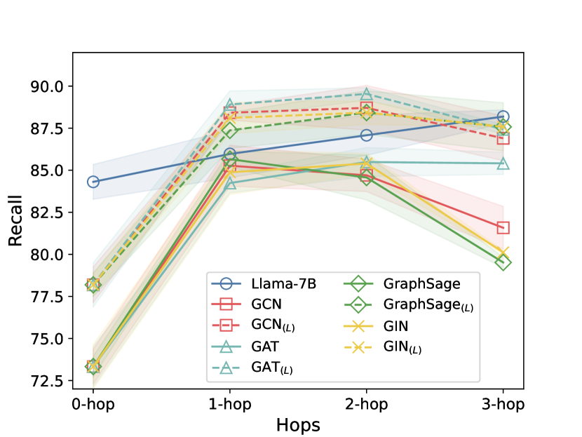
(b) Recall

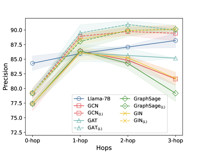
(c) Precision

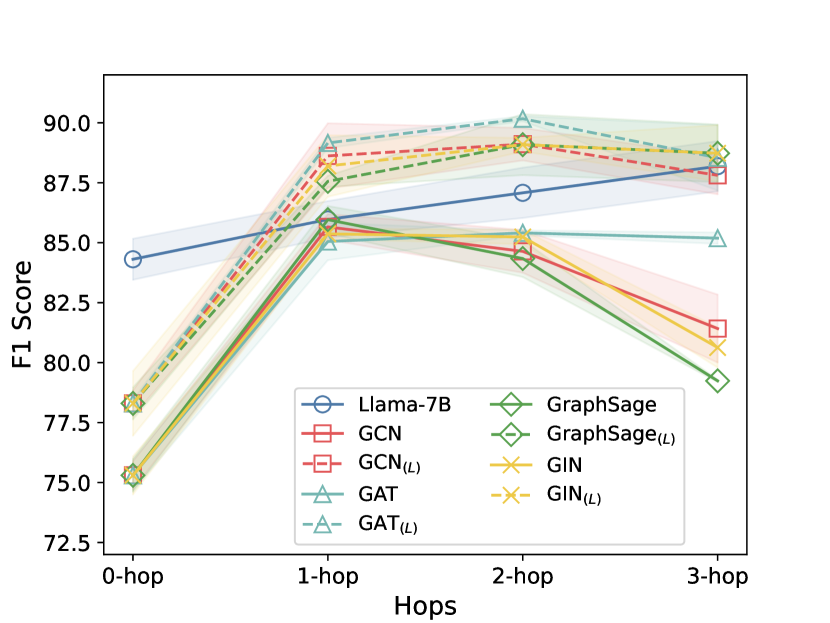
(d) F1

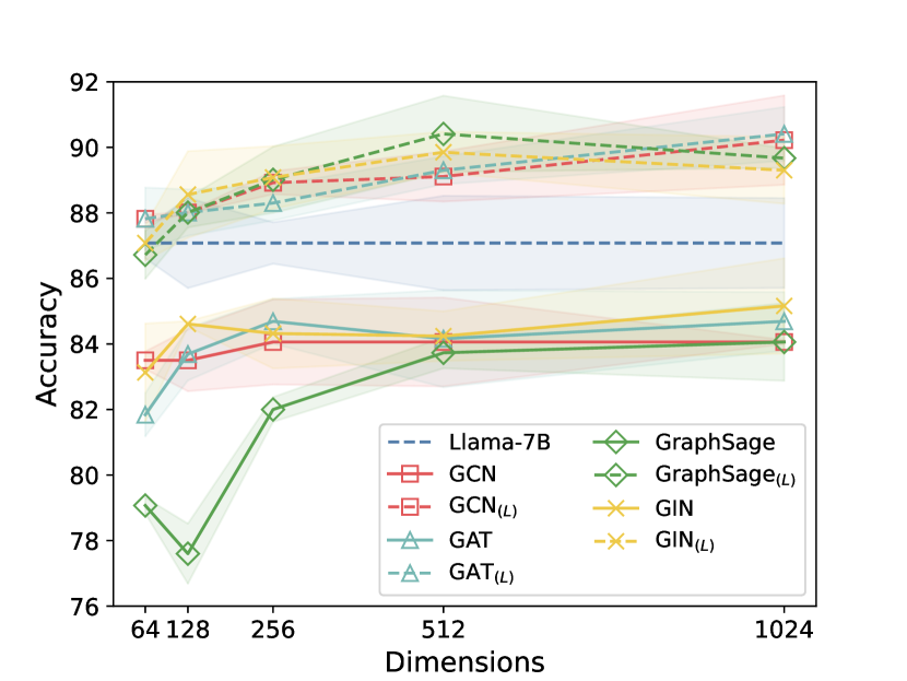
(e) Accuracy

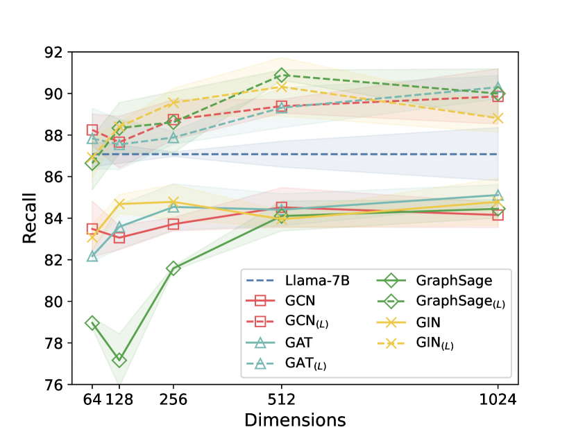
(f) Recall

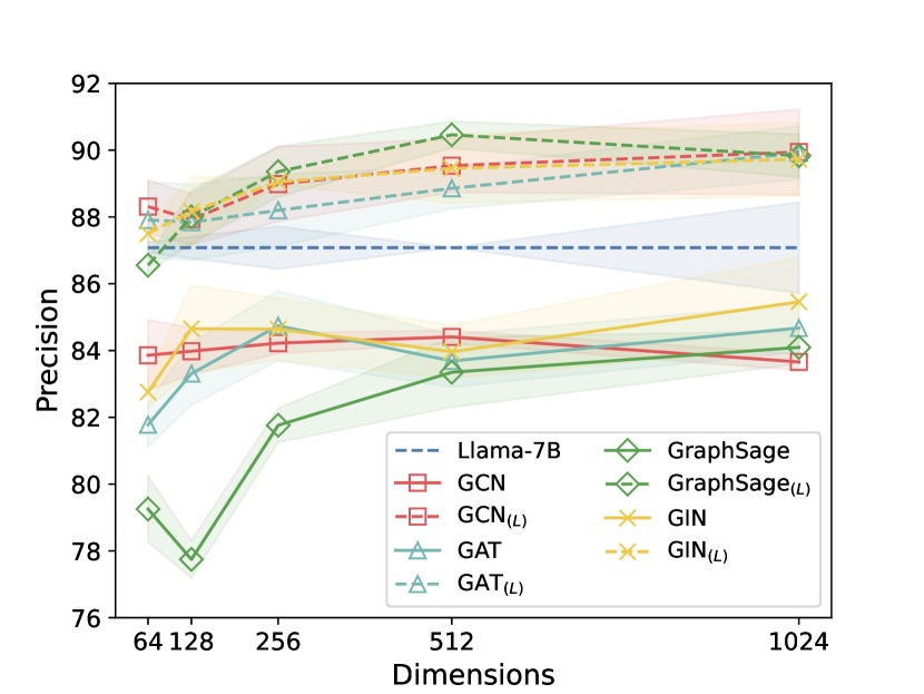
(g) Precision

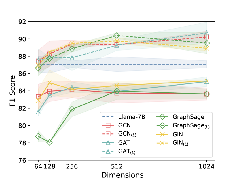
(h) F1

Figure 4. The results of performance impacts as the variations of neighbor orders and hidden feature dimension

4.1. Datasets and Backbone Models

Datasets

Our experiments employ three benchmark graph learning datasets: Arxiv (Hu et al., 2020), Cora, and PubMed (Yang et al., 2016), to evaluate the LinguGKD framework in node classification tasks. These datasets represent academic papers as nodes, with edges indicating citations. Node attributes include titles and abstracts, capturing the essence of each paper. Comprehensive dataset statistics are in Table 1. The detailed dataset descriptions are supplemented in Appendix B.

For the student GNN training, we utilized the preprocessed numerical node attributes provided in each dataset. However, for the teacher LLM’s fine-tuning, we reconstructed the complete textual content of node titles and abstracts following He et al.’s methodology (He et al., 2023) due to the datasets’ lack of extensive textual data.

Backbone Models

Our experiments utilized well-established LLMs and GNNs. As teacher models, we chose Llama2-7B (Touvron et al., 2023) and Mistral-7B (Jiang et al., 2023). For student GNNs, we selected GCN (Hamilton et al., 2017), GAT (Veličković et al., 2018), GraphSAGE (Hamilton et al., 2017), and GIN (Xu et al., 2019), known for their effectiveness in graph-based tasks. Detailed introductions to these competing models are provided in Appendix C.

4.2. Experimental Results and Analyses

Model Performance Analyses

To validate the robustness of our experimental findings, we conducted five separate runs with different random seeds, reporting mean metrics including accuracy, precision, recall, and F1 score (Appendix D provides detailed settings). Table 2 succinctly shows the node classification performance of various teacher LLMs and student GNNs across selected datasets. We have distinguished the top results in the table: the highest-performing outcomes are in bold, the best scores among LLMs are in italics, and those leading among GNNs are highlighted with a grey background. The notation GNN_(L) refers to GNN models distilled using Llama-7B as the teacher, while GNN_(M) indicates distillation with Mistral-7B. Gains reflects the performance improvement of teacher LLMs over the most effective baseline GNN. Gains_s and Gains_t represent the average gains in performance for distilled GNNs compared to baseline models and their respective LLM teachers, respectively.

The experimental findings highlight that LLMs, particularly Llama-7B, consistently outperform traditional GNNs in node classification tasks. Notably, Llama-7B achieved a significant 94.09% accuracy on PubMed, surpassing the GCN model’s 86.12%. It demonstrates the superior capability of instruction fine-tuned LLMs in understanding complex graph structures and node semantics. The dataset characteristics notably influence model performance; for instance, the focused topics of Cora and PubMed aid in semantic pattern recognition, while Arxiv’s broader scope presents more challenges in discerning node and graph relationships. Furthermore, regarding performance enhancement, LLMs exhibited varying degrees of improvement over GNNs, with Llama-7B showing a 7.08% performance increase on PubMed and a 4.98% rise on Arxiv. This variance highlights the impact of each dataset’s structural complexity and feature richness on LLMs’ semantic interpretation abilities.

Moreover, implementing LLMs in knowledge distillation has significantly enhanced GNN models. For example, GAT_(L), influenced by Llama-7B, attained a 91.15% accuracy on Cora, improving from the original GAT’s 86.12%. It suggests the effective transfer of LLMs’ intricate feature representations to GNNs, thereby enhancing their performance. Interestingly, in some cases, distilled GNNs even surpass their LLM teachers, as seen with GAT_(L) on Cora, which outperformed Llama-7B. However, it is not consistently observed across all datasets, likely due to the inherent differences in graph structures and the distillation strategies employed.

Application Trade-off of LinguGraph LLM vs. Distilled GNN

As shown in Figure 2, the right y-axis delineates the parameter quantity and storage requirements of various models through a line graph. In contrast, the left y-axis showcases the inference latency for these models across different datasets via a bar graph.

Concerning the number of model parameters, we reveal that while LLMs like Llama-7B and Mistral-7B encompass approximately 7 billion parameters, traditional GNNs range from 7 million to 11 million parameters, depending on the design difference of their message-passing layers. The vast disparity highlights GNNs’ significant edge in resource efficiency and model compactness, with their parameter count being merely 0.1% of that of LLMs.

Regarding inference latency, LLMs consistently exhibit longer durations across all evaluated datasets, with times largely influenced by the length of the prompts. On the other hand, GNNs achieve significantly shorter inference time. Nevertheless, the increase in graph data size can affect their speed. The application of graph sampling strategies for large-scale graphs has been effective in preserving the quick inference capabilities of GNNs, even when LLMs require up to 24 times longer in certain scenarios. It underscores the advantage of GNNs in scenarios demanding quick response times.

From the above analyses, while TAG instruction fine-tuned LLMs tend to reach high levels of predictive accuracy, distilled GNNs stand out for their lower computational and storage demands, alongside quicker inference capabilities at the expense of slightly reduced accuracy on several datasets. Thus, decision-makers are presented with a crucial choice: opting for the superior predictive performance of LLMs or favoring the efficient model inference of distilled GNNs. Carefully considering these trade-offs in the context of specific application requirements is essential for achieving the most effective and efficient outcomes.

Convergence Efficiency of GNNs vs. Distilled GNNs

Figure 3 illustrates the training convergence trajectories for a variety of distilled GNNs alongside their original ones, using the Cora as a benchmark dataset. Our observations reveal a dual advantage: not only do distilled GNNs exhibit superior performance, but they also achieve this excellence at a faster rate. This acceleration in convergence is a direct testament to the efficacy of our framework’s layer-adaptive semantic-structural alignment coupled with precise node classification tactics.

In conclusion, the proposed LinguGKD framework introduces a paradigm shift in the scalability and practical deployment of graph inference models, especially within large-scale environments. By striking for an optimal balance between computational efficiency and model performance, LinguGKD paves the way for more robust, faster-converging graph neural networks that do not compromise on their predictive accuracy.

4.3. Performance Impact of Hyperparameter

Based on the Cora dataset, we investigated how varying hyperparameters, specifically neighbor orders $k$ and hidden feature dimensions $d$ of GNNs, affects model performance of node classification in TAG. The hidden feature dimensions of the teacher LLMs are keeping at a constant 4096, as per the original model design.

Figure 4(a)-4(d) reveal that teacher LLMs consistently outperformed GNNs, regardless of neighbor orders, highlighting their superior semantic processing ability. Notably, even with no neighbor information (0-hop), LLMs showed a significant edge over GNNs. Under the LinguGKD framework, distilled GNNs surpassed original GNNs in all neighbor order settings, demonstrating the effective transfer of multi-order knowledge from LLMs to GNNs. However, while LLMs benefitted from increasing neighbor orders, GNNs experienced performance declines past the 2-hop mark due to over-smoothing. Distilled GNNs alleviated this issue but faced longer fine-tuning times for teacher LLM with increased order, leading us to choose a 2-hop setting for a balance of efficiency and effectiveness.

Figure 4(e)-4(h) provide insights into the impact of hidden feature dimensions on model performance. Original GNNs improved up to a 128-dimension limit, beyond which their performance plateaued. In contrast, distilled GNNs continued to show enhanced performance with higher dimensions, owing to their improved capacity for semantic and structural understanding from LLMs. Consequently, we set the hidden feature dimension at 1024 in our experiments to maximize the benefits from the teacher models.

For more detailed ablation experiments and parameter analysis, please refer to Appendix E.

5. Related Work

This section offers a succinct summary of pertinent research in LLM-based graph learning (He et al., 2023; Wei et al., 2024; Huang et al., 2023) and graph knowledge distillation (Ahluwalia et al., 2023; Samy et al., 2023; Yang et al., 2023).

Recent breakthroughs in graph learning have significantly benefited from incorporating LLMs, marking a transformative evolution in the domain. These advancements primarily fall into two categories: LLM as Enhancer (LaE) and LLM as Predictor (LaP), distinguished by their integration with graph data. The LaE strategy focuses on augmenting node embeddings in GNNs through LLMs’ semantic processing prowess, addressing traditional GNN limitations in extracting semantic features from TAGs. Techniques like TAPE (He et al., 2023), KEA (Chen et al., 2024), and LLM4Mol (Qian et al., 2023) exemplify this approach by enriching graph nodes with deeper semantic layers using LLM-generated annotations, knowledge entities, and molecular biology interpretations. In contrast, LaP methods directly leverage LLMs for graph inference tasks, such as classification. This includes Graphormer (Ying et al., 2021), which integrates graph data into Transformers, and SAT (Chen et al., 2022b), which embeds structural information into self-attention mechanisms. Additionally, initiatives like (Wang et al., 2024) and (Fatemi et al., 2023) explore LLMs’ capacity to encode graph structures in natural language, highlighting their potential and challenges in complex graph reasoning. Collectively, these studies illustrate the growing role of LLMs in graph learning, offering novel ways to decipher semantic content and complex graph structures.

In graph knowledge distillation, transferring complex knowledge from teacher models to simpler student models significantly boosts GNNs’ performance and efficiency. This field broadly encompasses three focal areas: distillation of output logits, latent features, and graph structures. Distillation of output logits, exemplified by the SGKD (He and Ma, 2022), ABKD (Ahluwalia et al., 2023), and model extraction attacks on GNNs (Wu et al., 2022), focuses on transferring final output representations to enhance student models’ accuracy and compression. Meanwhile, latent feature distillation, including Structure-Aware MLPs (Chen et al., 2022a), the Graph2Feat method (Samy et al., 2023), and graph contrastive representation distillation (G-CRD) (Joshi et al., 2022), targets the transfer of intermediate representations, aligning student node embeddings with teacher models in shared spaces. The third area, graph structure distillation, as seen in PGKD (Wu et al., 2023), graph-free knowledge distillation (Deng and Zhang, 2021), and VQGraph (Yang et al., 2023), focuses on imparting structural information, even achieving state-of-the-art GNN-MLP distillation results.

However, leveraging LLM-based approaches in graph knowledge distillation remains underexplored, particularly due to the contrasting nature of generative LLMs and discriminative GNNs. Our LinguGKD framework bridges this gap, employing a layer-adaptive contrastive strategy to align LLMs and GNNs within a latent space, significantly enhancing GNNs’ predictive accuracy and convergence rate and leading to potential feasibility for real applications.

6. Conclusion

In this paper, we explored the novel concept of using LLMs as teacher models for graph knowledge distillation, with a focus on node classification in TAG. First, treating node classification as a pure text generation task, we fine-tuned a pre-trained LLM, achieving expected classification performance in generating node labels through natural language processing of textual attributes and neighborhood structures. To resolve the storage issue of large model parameters and long inference latencies inherent in LLMs, we introduced the LinguGKD framework, which distills complex graph structure knowledge from the LLM into a more efficient student GNN. The distilled GNN, featuring a unique layer-adaptive semantic-structural alignment, has shown considerable improvements in node semantics comprehension and structure interpretation over traditional GNNs. Our experiments across diverse datasets demonstrated LinguGKD’s ability to enhance the distilled GNN’s node classification performance in TAG significantly, maintaining a trade-off between the effectiveness and efficiency compared to both teacher LLMs and student GNNs.

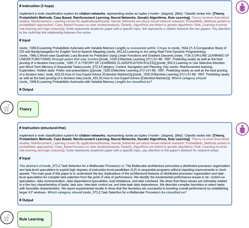
Figure 5. Node classification dialogue between a user and the LinguGraph LLM on the Cora dataset.

Appendix A Prompts

Figure 5 showcases a node classification dialogue between a user and the LinguGraph LLM on the Cora dataset. The right side of the figure displays the user’s instruction prompt, while the left side shows LinguoGraph LLM’s responses. This figure demonstrates how instruction $\mathcal{I}$, structural prompt $\tau$, and query $\mathcal{Q}$ are distinctively linked using markdown title syntax: “# Instruction \n {{$\mathcal{I}$}} \n # Input \n {{$\mathcal{\tau}$}}. {{$\mathcal{Q}$}} \n # Output”. The initial conversation pertains to classifying a node identified by id 1006 within the Cora dataset. The instruction portion highlighted in red signifies the human-summarized prior knowledge intended to direct the LLM in label prediction, incorporating the 3-hop neighbor subgraph of the focal node into the structural prompt. A subsequent dialogue reveals an example under a structure-unaware context, where the structural prompt diverges from encoding neighbor structures, predominantly presenting a synopsis of the focal node for LLM-based node classification context.

To address the challenge of exponential neighbor node increase with hop count and the pre-trained LLM’s text length limit, in our experimental setup for the $k$-hop neighbor subgraph $\mathcal{G}^{(k)}$ of the central node, we systematically sample a $k$th-hop neighbor and its shortest path to the central node iteratively, encoding this into the structural prompt in natural language, until reaching the predetermined maximum length threshold $\delta$. For every $l$-hop subgraph $\mathcal{G}^{(l)}\in\mathcal{G}^{k}$, this process is replicated $\theta$ times to compile an $l$th-hop instruction prompt ensemble $\mathcal{P}_{l}=\{\textbf{p}_{l}^{1},\dots,\textbf{p}_{l}^{\theta}\}$, illustrating the topology between the central node and its neighbors. This method enriches instruction prompt variety and aims to reduce bias in the LLM’s structural understanding due to sampling constraints.

Appendix B Datasets

Detailed descriptions of the datasets are as follows:

• Cora: The Cora dataset is a smaller academic citation network with a concentration on machine learning papers. It comprises approximately 2,700 papers, categorized into 7 groups that cover diverse branches of machine learning such as neural networks, probabilistic methods, and genetic algorithms.

• PubMed: Comprising 19,717 scientific publications related to diabetes from the PubMed database, the PubMed dataset is segmented into three groups: experimentally induced diabetes, Type 1 diabetes, and Type 2 diabetes. It features a citation network with 44,338 links.

• Arxiv: The Arxiv dataset represents a large academic citation network focusing on papers in natural language processing and computer vision. It includes over 170,000 papers, spanning research from 2007 to the present, and the papers are classified into 40 distinct categories representing various sub-disciplines within computer science.

Appendix C Backbone Models

Large Language Models

• Llama2-7B (Touvron et al., 2023): Llama2-7B is an auto-regressive pretrained language model with 7 billion parameters that uses an optimized transformer architecture, developed and publicly released by Meta. It is pretrained on 2 trillion tokens of data from publicly available sources, which has a cutoff of September 2022.

• Mistral-7B (Jiang et al., 2023): Mistral 7B is developed by the Mistral AI team, which is a cutting-edge LLM with 7.3 billion parameters utilizing Grouped-query attention (GQA) (Ainslie et al., 2023) and Sliding Window Attention (SWA) (Beltagy et al., 2020) for efficient processing.

Graph Neural Networks

• GCN (Hamilton et al., 2017): Graph Convolutional Network (GCN) revolutionize graph analysis by extending convolutional neural networks to graph-structured data, enabling node feature learning through neighborhood aggregation. GCN efficiently captures local graph topology and node features in a fixed-length vector, facilitating tasks like node classification and link prediction. The model’s strength lies in its ability to learn complex relational patterns through layers of graph convolutions, making it highly effective for semi-supervised learning on large-scale graphs. This architecture innovates by generalizing traditional convolution operations to the graph domain, leveraging the eigendecomposition of graph Laplacians for scalable and powerful representation learning.

• GAT (Veličković et al., 2018): Graph Attention Network (GAT) introduce a novel approach to graph neural network architectures by incorporating attention mechanisms that operate on graph-structured data. This method addresses the limitations of previous models based on graph convolutions or approximations by leveraging masked self-attention layers. In GAT, nodes are capable of attending over their neighborhoods’ features with varying degrees of importance, implicitly allowing for the assignment of different weights to different nodes within a neighborhood without the need for expensive matrix operations or prior knowledge of the graph structure. This key innovation enables GATs to simultaneously tackle several challenges of spectral-based graph neural networks, rendering the model applicable to both inductive and transductive problems.

• GraphSAGE (Hamilton et al., 2017): GraphSAGE is an innovative graph neural network framework that enables inductive representation learning by leveraging node feature information to generate node embeddings for unseen data during training. Unlike transductive methods that require re-training for new nodes, GraphSAGE uses a novel sampling and aggregation strategy to learn a function that generates embeddings by sampling and aggregating features from a node’s local neighborhood. Its aggregation functions, which can be mean, LSTM, pooling, or other custom functions, allow GraphSAGE to effectively capture the structural context of nodes within large and complex graph structures. This framework supports various downstream tasks such as node classification and link prediction, demonstrating superior adaptability and scalability across diverse graph datasets.

• GIN (Xu et al., 2019): The Graph Isomorphism Network (GIN) enhances graph neural networks by merging a node’s features with its neighbors’ features using a customizable, nonlinear function. This unique aggregation technique allows GIN to accurately identify various graph structures, ensuring it maintains the graph’s isomorphic characteristics. Essentially, the model is built on the principle that its ability to differentiate between any two distinct (non-isomorphic) graphs indicates a high level of expressive strength. By emulating the discriminative capability of the Weisfeiler-Lehman graph isomorphism test, GIN significantly boosts graph neural networks’ efficiency in recognizing intricate graph structures, positioning it as a powerful tool for complex graph analysis tasks.

Appendix D Hyperparameter Settings

Our experimental framework was executed on a workstation equipped with an NVIDIA GTX 4090 GPU, along with an Intel(R) Xeon(R) Gold 6130 CPU, and 1T of RAM. The experimental suite for LinguGKD was developed using Python 3.9.6, PyTorch 2.0.1, and CUDA 12.0, ensuring compatibility and performance optimization.

Table 3. Overview of experimental settings.

Symbol	Description	Value(s)
$\mathcal{D}_{tr}$	Training set	3:1:1 split for Cora and PubMed, 6:2:3 split for Arxiv
$\mathcal{D}_{val}$	Validation set
$\mathcal{D}_{t}$	Test set
$\theta$	Number of instruction prompts per hop	2
$N_{Cora}$	Total prompts for Cora	62,216
$N_{PubMed}$	Total prompts for PubMed	121,580
$N_{Arxiv}$	Total prompts for Arxiv	100,123
$s_{max}$	Maximum sequence length	512
$d_{L}$	Hidden feature dimension for LinguGraph LLM	4096
$mb_{L},mb_{G}$	Training Mini-batch size for LLMs and GNNs	2 for LLMs, 32 for GNNs
$g_{acc}$	Gradient accumulation	2
$\eta_{L},\eta_{G}$	Learning rate for LLMs and GNNs	1e-4 for LLMs, 1e-3 for GNNs
$ep_{L},ep_{G}$	Training epochs for LLMs and GNNs	1 for LLMs, 100 for GNNs
$lora_{r}$	LoRA parameter	64
$lora_{\alpha}$	LoRA alpha	32
$d_{G}$	Feature dimension of GNN	[64, 128, 256, 512, 1024]
$d_{k}$	Dimension of distilled knowledge	Matches $d_{G}$

Dataset Splitting

For dataset partitioning, we applied a 3:1:1 division ratio to both the Cora and PubMed datasets, categorizing them into training $\mathcal{D}_{tr}$, validation $\mathcal{D}_{val}$, and test sets $\mathcal{D}_{t}$. This splitting strategy is in line with methods detailed in prior studies (Ye et al., 2024). For the Arxiv dataset, a different split ratio of 6:2:3 was adopted, conforming to publicly recommended guidelines (Yang et al., 2016). We assessed the models’ performance using four established metrics: node classification accuracy, precision, recall, and Macro F1 score. These metrics collectively provide a comprehensive view of each model’s effectiveness in correctly classifying nodes within the graph, balancing the precision of positive predictions against their recall and offering an aggregated measure of performance through the Macro F1 score.

Instruction Tuning of PLM

During the LLM’s fine-tuning phase, we utilized pre-trained models from huggingface.co. The LLM input’s maximum sequence length $s_{max}$ was capped at 512, accommodating a hidden feature dimension $d_{L}$ of 4096. Training settings included a minimal batch size $mb_{L}$ of 2, gradient accumulation $g_{acc}$ also set at 2, and a modest learning rate $\eta_{L}$ of 1e-4, all within a concise training duration $ep_{L}$ of 1 epoch. For each center node $v_{i}$, we defined a maximum neighboring subgraph order $k$ of 3, constructing instruction prompts $\mathcal{P}=\{\mathcal{P}_{0},\mathcal{P}_{1},\mathcal{P}_{2},\mathcal{P}_{3}\}$ to cover structural prompts from 0 to 3-hop subgraphs.

Considering the computational and storage constraints, for the large-scale Arxiv dataset, we opted for a practical approach by randomly sampling 5% of nodes in practice. We standardized the number of instruction prompts per hop ($\theta$) at 2, culminating in totals of 62,216, 121,580, and 100,123 instruction prompts for Cora, PubMed, and Arxiv, respectively. Despite the fact that 2 instruction prompts typically do not provide a comprehensive description of the entire $l$-hop subgraph structure, our experimental findings underscore the PLMs’ exceptional capability for learning from minimal data samples. This necessitates merely sparse representations of subgraph structures to effectively fine-tune PLMs, thereby equipping them with an understanding of node semantics and their interconnectivity with adjacent nodes. Such an approach significantly enhances the LLM’s proficiency in making precise node classification predictions.

In the fine-tuning process, we integrated LoRA and 4-bit quantization techniques, with LoRA’s parameters set to $lora_{r}$=64, dropout at 0.1, and alpha $lora_{\alpha}$ to 32. This adjustment resulted in a total of approximately 1,800,000 trainable parameters, including elements like q_proj, k_proj, v_proj, o_proj, and lm_head.

In the node label generation steps of LinguGraph LLM, each node underwent classification for every instructional prompt via a greedy search algorithm. Then a majority voting scheme was applied, where the most frequently appearing classification across prompts was selected as the final prediction, ensuring a balanced and democratically derived outcome.

Graph Knowledge Distillation

In the distillation of graph knowledge from LinguGraph LLM to GNNs, we utilized various GNN architectures implemented through PyG. Across all benchmark datasets, we standardized the learning rate $\eta_{G}$ at 1e-3, batch size $mb_{G}$ at 32, and extended the training to 100 epochs ($ep_{G}$). The performance of our LinguGKD was assessed across different message-passing layers [0, 1, 2, 3]. For simplicity in our experiments, we aligned the feature dimension of the GNN, denoted as $d_{G}$, with that of the distilled knowledge, $d_{k}$. Then we explored the effects of varying the hidden feature dimensions of GNNs and distilled knowledge at [64, 128, 256, 512, 1024].

For each central node $v_{i}$ within a specified neighbor order $l$, our experimental setup involved generating $\theta$ unique instruction prompts. This led to the extraction of $\theta$ $l$-hop features $\{\textbf{f}_{l,(1)}^{L},\dots,\textbf{f}_{l,(\theta)}^{L}\}$ from the LinguGraph LLM for $v_{i}$. During the layer-adaptive knowledge distillation phase, we leveraged a pooling operation—either max pooling or average pooling—to amalgamate these features into a consolidated feature representation $\textbf{f}_{l}^{L}$ that accurately reflects the $l$-th order neighborhood’s characteristics.

Appendix E Experimental Analysis

Table 4. Node classification performance comparison of various GNN models distilled with and without layer-adaptive graph knowledge distillation on Cora & PubMed.

		1-hop				2-hop				3-hop
		Acc.	Prec.	Recall	F1	Acc.	Prec.	Recall	F1	Acc.	Prec.	Recall	F1
GCN${}_{(L)}^{-}$	Cora	89.48	88.65	89.20	88.89	90.04	89.43	89.80	89.56	89.10	89.12	89.21	89.12
GCN(L)		89.48	88.79	88.56	88.66	90.41	90.21	90.70	90.37	89.67	89.28	89.85	89.50
Gains		0.00%	0.16%	-0.72%	-0.26%	0.41%	0.87%	1.00%	0.90%	0.64%	0.18%	0.72%	0.43%
GAT${}_{(L)}^{-}$		89.67	89.06	89.38	89.16	90.22	90.57	89.78	90.14	90.22	89.38	90.14	89.58
GAT(L)		90.04	90.05	88.56	89.23	90.77	89.78	91.57	90.60	90.22	90.21	90.84	90.47
Gains		0.41%	1.11%	-0.92%	0.08%	0.61%	-0.87%	1.99%	0.51%	0.00%	0.93%	0.78%	0.99%
GraphSAGE${}_{(L)}^{-}$		88.93	87.95	88.18	88.01	88.38	87.29	87.41	87.27	87.45	87.56	86.61	86.99
GraphSAGE(L)		90.22	90.22	89.67	89.83	90.22	89.46	89.44	89.41	89.3	89.35	88.69	89.01
Gains		1.45%	2.58%	1.69%	2.07%	2.08%	2.49%	2.32%	2.45%	2.12%	2.04%	2.40%	2.32%
GIN${}_{(L)}^{-}$		88.75	87.02	88.79	87.78	88.19	87.25	88.61	87.88	87.45	86.61	87.98	87.25
GIN(L)		88.75	87.93	88.14	88.00	89.48	88.72	89.76	89.18	88.38	85.46	90.78	87.55
Gains		0.00%	1.05%	-0.73%	0.25%	1.46%	1.68%	1.30%	1.48%	1.06%	-1.33%	3.18%	0.34%
GCN${}_{(L)}^{-}$	PubMed	87.85	87.39	87.19	87.27	88.00	87.45	87.69	87.56	87.39	87.21	86.93	87.11
GCN(L)		88.18	87.45	87.79	87.64	88.95	88.16	88.69	88.41	88.53	88.45	88.13	88.37
Gains		0.38%	0.07%	0.69%	0.42%	1.08%	0.81%	1.14%	0.97%	1.30%	1.42%	1.38%	1.45%
GAT${}_{(L)}^{-}$		87.73	86.72	87.20	87.10	86.92	85.12	85.40	85.27	85.78	85.39	85.89	85.58
GAT(L)		87.85	87.28	87.45	87.36	86.97	85.96	86.59	86.25	86.97	85.96	86.59	86.25
Gains		0.14%	0.65%	0.29%	0.30%	0.06%	0.99%	1.39%	1.15%	1.39%	0.67%	0.81%	0.78%
GraphSAGE${}_{(L)}^{-}$		89.33	88.66	89.17	89.02	89.63	88.55	89.96	89.17	89.23	88.18	89.12	88.75
GraphSAGE(L)		89.68	89.54	89.23	89.38	89.98	89.89	89.57	89.72	89.59	89.39	89.69	89.48
Gains		0.39%	0.99%	0.07%	0.40%	0.39%	1.51%	-0.43%	0.62%	0.40%	1.37%	0.64%	0.82%
GIN${}_{(L)}^{-}$		86.32	85.96	86.01	85.98	87.13	85.94	86.61	86.42	86.13	85.17	85.51	85.37
GIN(L)		87.60	86.78	87.28	87.01	87.50	86.29	87.58	86.86	87.21	86.19	87.31	86.73
Gains		1.48%	0.95%	1.48%	1.20%	0.42%	0.41%	1.12%	0.51%	1.25%	1.20%	2.11%	1.59%

Ablation Study

In Section 3.2.3, we emphasized that encoding features of neighbors at different orders holds varying importance across different downstream tasks, for which we proposed a layer-adaptive knowledge distillation strategy. Here, we design additional ablation experiments to compare the effects of adopting versus not adopting the layer-adaptive knowledge distillation strategy on the effectiveness of our proposed LinguGKD. We constructed a variant of LinguGKD, named LinguGKD-, which only aligns the last-order node features extracted by LinguGraph LLM as graph knowledge with the features output by the last layer’s message-passing layer of GNN in the distillation space. We used the instruction fine-tuned Llama-7B as the teacher model and conducted comparative experiments on the Cora and PubMed datasets, with results shown in 4. Here, GNN${}_{(L)}^{-}$ denotes the GNNs distilled via the LinguGKD- framework.

We can find that distilled GNNs obtained through the LinguGKD framework outperform those distilled via the LinguGKD- framework in the vast majority of experimental setups, validating our hypothesis. Specifically, on the Cora dataset, all GNN variants showed performance improvements on nearly all evaluation metrics after adopting layer-adaptive knowledge distillation. Notably, GraphSAGE showed significant improvements in accuracy, precision, recall, and F1 score in the 2-hop scenario, with increases of 2.08%, 2.49%, 2.32%, 2.45%, respectively. On the PubMed dataset, performance improvements were similarly observed, with GIN showing the most significant increase in accuracy, reaching 1.48%. The results indicate that distilling features of neighbors at different levels can effectively enhance the model’s generalization ability and performance. This is because information on different levels of graph structure holds varying importance for different downstream tasks, and the layer-adaptive strategy can better capture and utilize this information. The benefits of this strategy vary for different GNN architectures, which may relate to each model’s sensitivity and approach to processing graph structural information. For example, GraphSAGE shows more significant performance improvements in certain scenarios, possibly due to information loss caused by its sampling strategy.

The experiments also displayed performance variations under different hop numbers (1-hop, 2-hop, 3-hop), with the benefits of the layer-adaptive knowledge distillation strategy increasing with the number of hops. This suggests that focusing on node semantics (lower-order features) while capturing more neighbor information is beneficial. These results verify the effectiveness of the layer-adaptive knowledge distillation strategy in improving GNN performance and also emphasize the necessity of considering the hierarchical structure of graphs and the importance of different neighbors when designing GNN models and distillation strategies.

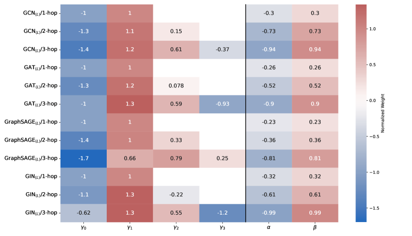
(a) Cora

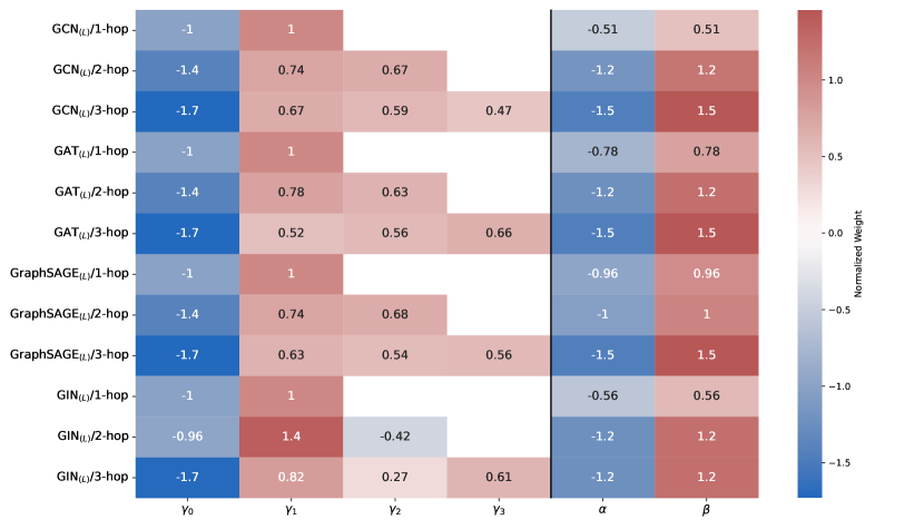
(b) PubMed

Figure 6. A heatmap visualization of the normalized layer-adaptive factors $\gamma_{l}$ and classification-distillation loss weights $\alpha$ and $\beta$ during the training of distilled GNN models on Cora and PubMed datasets.

Adaptive Weight Analysis

To delve into the significance of teacher model insights across different neighborhood orders in the distillation process, as well as the effects of distillation loss ($\mathcal{L}_{D}$) and node classification loss ($\mathcal{L}_{G}$) on GNN training, we employed a heatmap visualization. This visualization, depicted in 6, showcases the normalized layer-adaptive factors $\gamma_{l}$ for layers (or hops) 0 through 3, alongside the weights for classification-distillation loss, $\alpha$ and $\beta$, across the Cora and PubMed datasets.

The heatmap elucidates that, in most experimental scenarios, the 1-hop teacher knowledge is paramount. This level of knowledge, as distilled by the LinguGraph LLM, represents an optimal blend of node semantics and structural insights, crucially enhancing node classification. The reliance on broader neighborhood insights shifts with the dataset context; notably, the PubMed dataset demonstrates a heightened dependency on extended neighbor relations compared to Cora. This trend likely stems from the thematic closeness of PubMed papers, where broader citation contexts more substantially influence topic predictions.

Regarding loss weights, the heatmap indicates a consistent prioritization of the distillation loss across setups, suggesting a focused emulation of the teacher model’s insights by the student GNN. This approach underscores the success of our LinguGKD framework, emphasizing that mimicking the teacher model’s behavior through strategic loss weighting can significantly uplift the distilled GNN’s performance. This analysis not only affirms the value of the LinguGKD strategy but also illustrates the nuanced role of neighbor order knowledge and loss weighting in training GNNs for enhanced predictive accuracy.

Appendix F Related Work

In this section, we provide a concise overview of the related research intimately connected to this study, examining it from two distinct perspectives: LLM-based graph learning (He et al., 2023; Wei et al., 2024; Huang et al., 2023) and graph knowledge distillation (Ahluwalia et al., 2023; Samy et al., 2023; Yang et al., 2023).

F.1. LLMs based Graph Learning

Recent advancements in graph learning have been significantly enriched by the integration of LLMs, marking a notable evolution in the field. Research in this domain can be primarily categorized into two distinct approaches: LLM as Enhancer (LaE) (He et al., 2023; Chen et al., 2024; Wei et al., 2024) and LLM as Predictor (LaP) (Wang et al., 2024; Fatemi et al., 2023; Ye et al., 2024), distinguished by their degree of integration with graph-structured data.

The LaE approach improves node embedding quality in GNNs by harnessing the semantic processing capabilities of LLMs. This enhancement, when incorporated into the graph’s structure, effectively addresses the limitations in traditional GNNs, particularly their shortcomings in semantic feature extraction from TAGs. One specific implementation of the LaE approach is the TAPE (He et al., 2023). TAPE utilizes LLMs to generate interpretive explanations and pseudo-labels, enriching the graph’s textual attributes. This is augmented by fine-tuning a smaller-scale language model with both the original text and these generated annotations, thereby transforming textual semantics into robust node embeddings. This technique leverages the deep semantic comprehension of LLMs, infusing nodes with enhanced informational depth. Following this, Chen et.al (Chen et al., 2024) propose the Knowledge Entity Augmentation (KEA) strategy that employs LLMs to generate lists of knowledge entities, complete with textual descriptions. These entities and their descriptions are encoded using a fine-tuned PLM and an advanced sentence embedding technique. KEA capitalizes on the LLMs’ ability to extract intricate semantic layers, thereby enriching the graph nodes with more nuanced semantic information. Qian et.al (Qian et al., 2023) involve using LLMs to produce detailed, semantically-rich interpretations of original strings, followed by fine-tuning a compact language model for downstream tasks. This method has shown considerable potential in areas such as pharmaceutical discovery and molecular biology. Lastly, Wei et.al (Wei et al., 2024) address the challenges of data scarcity and quality in graph-based recommendation systems. By enhancing user-item interaction edges through LLMs, it creates a more information-rich edge dataset. An efficient GNN model is then employed to encode this augmented recommendation network, significantly improving the system’s precision and effectiveness.

Furthermore, several studies have explored the direct application of LLMs in producing text-based node embeddings for GNNs. A notable example is the GIANT (Chien et al., 2022) method, which innovatively refines language models through a self-supervised learning framework. This method utilizes XR-Transformers (Zhang et al., 2021) to address the challenges of extreme multi-label classification in link prediction scenarios. Building on similar principles, Duan et.al (Duan et al., 2023) and Zhu et.al (Zhu et al., 2023) refine PLMs using link prediction analogues. This fine-tuning process enhances the structural awareness of the models, enabling them to better understand and process graph structures. Huang et.al (Huang et al., 2023) incorporate a graph-tailored adapter at the terminus of PLMs. This design facilitates the extraction of graph-aware node features. After training, they can generate interpretable node representations for a variety of tasks, leveraging tailored prompts to adapt to different scenarios. Lastly, Tan et.al (Tan et al., 2023) introduce an innovative unsupervised technique for universal graph representation learning. They create attribute-enriched random walks on graphs and convert these walks into coherent text sequences through an automated process. Subsequently, the LLM is fine-tuned using these sequences, allowing it to capture nuanced representations of the graph structure.

LaP methodologies fundamentally utilize LLMs for direct prediction tasks in graph-related contexts, including classification and inference. These approaches bifurcate into two distinct streams: one involves Transformer-based models specifically tailored for unique graph structures and trained directly on graph data, while the other utilizes PLMs to encode graph structures in natural language for direct inference. In the first stream, Graphormer (Ying et al., 2021) stands out by refining the conventional Transformer architecture with innovative structural encoding techniques. These enhancements enable it to integrate graph structural data seamlessly into the Transformer framework, significantly boosting its performance beyond that of traditional GNNs. Graphormer’s capabilities have been mathematically validated, demonstrating its role as a versatile and effective tool in graph representation learning, encompassing many GNN variants under its framework. Another notable development is the Structure-Aware Transformer (SAT) (Chen et al., 2022b), which focuses on integrating structural information into the self-attention mechanism of graph Transformers. Specifically, the SAT extracts subgraph representations rooted at each node before computing the attention, aiming to address the structural inductive biases in GNNs.

In the second stream, the focus shifts to leveraging the capabilities of LLMs pre-trained on large-scale corpora for encoding graph structures in natural language, thereby enabling direct graph inference. Research initiatives like (Wang et al., 2024) and (Fatemi et al., 2023), delve into the ability of LLMs to process textual descriptions of graphs. These studies, covering a spectrum of tasks from connectivity to emulating GNNs, shed light on the potential and limitations of LLMs in graph reasoning. They particularly underscore the challenges LLMs face in complex scenarios, especially when accidental correlations in graphs and problem constructs occur. Addressing these challenges, recent advancements focus on fine-tuning LLMs to enhance their understanding of graph structures. For example, Ye et.al (Ye et al., 2024) propose scalable prompting techniques based on maximal hop counts, effectively creating direct relational links between central and neighboring nodes through natural language expressions. This method has shown to outperform traditional GNNs in node classification tasks across various benchmark datasets.

Collectively, these advancements underscore the burgeoning potential of LLMs in graph learning, skillfully deciphering both semantic content and complex graph structures, and introducing innovative methodologies to the field.

F.2. Graph Knowledge Distillation

In the realm of graph knowledge distillation, the strategic transfer of intricate knowledge from complex teacher models to simpler student models is crucial for enhancing GNNs’ effectiveness and efficiency. This technique not only maintains the student model’s lightweight nature but also strives to emulate the teacher model’s advanced behavior. Predominantly, research in this field is categorized into three areas based on the type of knowledge distilled: output logits (He and Ma, 2022; Ahluwalia et al., 2023; Wu et al., 2022), latent features (Chen et al., 2022a; Samy et al., 2023; Joshi et al., 2022), and graph structure (Wu et al., 2023; Deng and Zhang, 2021; Yang et al., 2023).

Research focusing on output logits in graph knowledge distillation aims at transferring the final output representations from the teacher model to the student model. He et.al (He and Ma, 2022) proposed the Scalable and Effective Knowledge Distillation Framework for Graph Representation Learning (SGKD), which includes feature propagation to provide MLPs with graph structure-aware features and addresses unreliable logits of the teacher model. Ahluwalia et al. (Ahluwalia et al., 2023) introduced Attention-Based Knowledge Distillation (ABKD) for compressing large GNNs into smaller ones while maintaining accuracy, achieving a significant increase in accuracy with a substantial compression ratio. Wu et al. (Wu et al., 2022) developed an approach that focuses on model extraction attacks on GNNs, demonstrating effective duplication of models with high input-output correlation.

Latent feature distillation involves transferring intermediate representations from the teacher to the student model. Chen et al. (Chen et al., 2022a) proposed a Structure-Aware MLP student and a structure-mixing knowledge distillation strategy to distill knowledge from GNNs into Structure-Aware MLPs. The Graph2Feat method by Samy et al. (Samy et al., 2023) enables inductive link prediction in graph machine learning through knowledge distillation, showing superior performance in terms of AUC and average precision. Joshi et al. (Joshi et al., 2022) introduced graph contrastive representation distillation (G-CRD), aligning student node embeddings with those of the teacher in a shared representation space, thereby preserving global topology.

Distillation of graph structure knowledge focuses on transferring structural information from the teacher to the student model. Wu et al.’s Prototype-Guided Knowledge Distillation (PGKD) (Wu et al., 2023) method distills graph structural information from GNNs to MLPs without requiring graph edges. The graph-free knowledge distillation (GFKD) approach by Deng et al. (Deng and Zhang, 2021) models graph topology structures for knowledge transfer without using graph data. Yang et al. (Yang et al., 2023) proposed VQGraph, a framework that uses knowledge distillation to transfer structural knowledge from GNNs to MLPs, achieving new state-of-the-art performance on GNN-MLP distillation.

Despite these substantial insights, the exploration of LLM-based approaches in graph knowledge distillation has been limited, particularly due to structural differences between generative LLMs and discriminative GNNs. Addressing this gap, we introduce the LinguGKD framework, employing a layer-adaptive contrastive distilling strategy to align the graph structural features of LLMs and GNNs within a latent space. Our extensive experiments across various GNN architectures and benchmark datasets have validated LinguGKD’s ability to significantly enhance GNNs’ predictive accuracy and convergence rate without additional data or model parameters.

References

- (1)
- Ahluwalia et al. (2023) Anshul Ahluwalia, Rohit Das, Payman Behnam, Alind Khare, Pan Li, and Alexey Tumanov. 2023. ABKD: Graph Neural Network Compression with Attention-Based Knowledge Distillation. arXiv:2310.15938
- Ainslie et al. (2023) Joshua Ainslie, James Lee-Thorp, Michiel de Jong, Yury Zemlyanskiy, Federico Lebrón, and Sumit Sanghai. 2023. GQA: Training Generalized Multi-Query Transformer Models from Multi-Head Checkpoints. arXiv:2305.13245
- Beltagy et al. (2020) Iz Beltagy, Matthew E. Peters, and Arman Cohan. 2020. Longformer: The Long-Document Transformer. arXiv:2004.05150
- Chen et al. (2022b) Dexiong Chen, Leslie O’Bray, and Karsten Borgwardt. 2022b. Structure-Aware Transformer for Graph Representation Learning. In International Conference on Machine Learning (ICML), Vol. 162. 3469–3489.
- Chen et al. (2022a) Jie Chen, Shouzhen Chen, Mingyuan Bai, Junbin Gao, Junping Zhang, and Jian Pu. 2022a. SA-MLP: Distilling Graph Knowledge from GNNs into Structure-Aware MLP. arXiv:2210.09609
- Chen et al. (2024) Zhikai Chen, Haitao Mao, Hang Li, Wei Jin, Hongzhi Wen, Xiaochi Wei, Shuaiqiang Wang, Dawei Yin, Wenqi Fan, Hui Liu, and Jiliang Tang. 2024. Exploring the Potential of Large Language Models (LLMs) in Learning on Graphs. arXiv:2307.03393
- Chien et al. (2022) Eli Chien, Wei-Cheng Chang, Cho-Jui Hsieh, Hsiang-Fu Yu, Jiong Zhang, Olgica Milenkovic, and Inderjit S Dhillon. 2022. Node Feature Extraction by Self-Supervised Multi-scale Neighborhood Prediction. arXiv:2111.00064
- Deng and Zhang (2021) Xiang Deng and Zhongfei Zhang. 2021. Graph-Free Knowledge Distillation for Graph Neural Networks. In International Joint Conference on Artificial Intelligence (IJCAI). 2318–2324.
- Duan et al. (2023) Keyu Duan, Qian Liu, Tat-Seng Chua, Shuicheng Yan, Wei Tsang Ooi, Qizhe Xie, and Junxian He. 2023. SimTeG: A Frustratingly Simple Approach Improves Textual Graph Learning. arXiv:2308.02565
- Fatemi et al. (2023) Bahare Fatemi, Jonathan Halcrow, and Bryan Perozzi. 2023. Talk like a Graph: Encoding Graphs for Large Language Models. arXiv:2310.04560
- Hamilton et al. (2017) Will Hamilton, Zhitao Ying, and Jure Leskovec. 2017. Inductive Representation Learning on Large Graphs. In Advances in Neural Information Processing Systems (NeurIPS), Vol. 30.
- He et al. (2023) Xiaoxin He, Xavier Bresson, Thomas Laurent, Adam Perold, Yann LeCun, and Bryan Hooi. 2023. Harnessing Explanations: LLM-to-LM Interpreter for Enhanced Text-Attributed Graph Representation Learning. arXiv:2305.19523
- He and Ma (2022) Yufei He and Yao Ma. 2022. SGKD: A Scalable and Effective Knowledge Distillation Framework for Graph Representation Learning. In 2022 IEEE International Conference on Data Mining Workshops (ICDMW). 666–673.
- Honovich et al. (2022) Or Honovich, Thomas Scialom, Omer Levy, and Timo Schick. 2022. Unnatural Instructions: Tuning Language Models with (Almost) No Human Labor. arXiv:2212.09689
- Hu et al. (2020) Weihua Hu, Matthias Fey, Marinka Zitnik, Yuxiao Dong, Hongyu Ren, Bowen Liu, Michele Catasta, and Jure Leskovec. 2020. Open Graph Benchmark: Datasets for Machine Learning on Graphs. In Advances in Neural Information Processing Systems (NeurIPS), Vol. 33. 22118–22133.
- Huang et al. (2023) Xuanwen Huang, Kaiqiao Han, Dezheng Bao, Quanjin Tao, Zhisheng Zhang, Yang Yang, and Qi Zhu. 2023. Prompt-based Node Feature Extractor for Few-shot Learning on Text-Attributed Graphs. arXiv:2309.02848
- Hugging Face (2024) Hugging Face. 2024. Open LLM Leaderboard. https://huggingface.co/spaces/HuggingFaceH4/open_llm_leaderboard
- Jiang et al. (2023) Albert Q. Jiang, Alexandre Sablayrolles, Arthur Mensch, Chris Bamford, Devendra Singh Chaplot, Diego de las Casas, Florian Bressand, Gianna Lengyel, Guillaume Lample, Lucile Saulnier, Lélio Renard Lavaud, Marie-Anne Lachaux, Pierre Stock, Teven Le Scao, Thibaut Lavril, Thomas Wang, Timothée Lacroix, and William El Sayed. 2023. Mistral 7B. arXiv:2310.06825
- Joshi et al. (2022) Chaitanya K. Joshi, Fayao Liu, Xu Xun, Jie Lin, and Chuan Sheng Foo. 2022. On Representation Knowledge Distillation for Graph Neural Networks. IEEE Transactions on Neural Networks and Learning Systems (2022), 1–12.
- Kipf and Welling (2017) Thomas N. Kipf and Max Welling. 2017. Semi-Supervised Classification with Graph Convolutional Networks. arXiv:1609.02907
- Li et al. (2023) Jianxin Li, Hao Peng, Yuwei Cao, Yingtong Dou, Hekai Zhang, Philip S. Yu, and Lifang He. 2023. Higher-Order Attribute-Enhancing Heterogeneous Graph Neural Networks. IEEE Transactions on Knowledge and Data Engineering 35, 1 (2023), 560–574.
- Li et al. (2024) Yuhan Li, Zhixun Li, Peisong Wang, Jia Li, Xiangguo Sun, Hong Cheng, and Jeffrey Xu Yu. 2024. A Survey of Graph Meets Large Language Model: Progress and Future Directions. arXiv:2311.12399
- Li et al. (2022) Yanying Li, Xiuling Wang, Yue Ning, and Hui Wang. 2022. Fairlp: Towards fair link prediction on social network graphs. In International AAAI Conference on Web and Social Media (AAAI), Vol. 16. 628–639.
- OpenAI (2023) OpenAI. 2023. Prompt Engineering. https://platform.openai.com/docs/guides/prompt-engineering
- Ouyang et al. (2022) Long Ouyang, Jeffrey Wu, Xu Jiang, Diogo Almeida, Carroll Wainwright, Pamela Mishkin, Chong Zhang, Sandhini Agarwal, Katarina Slama, Alex Ray, John Schulman, Jacob Hilton, Fraser Kelton, Luke Miller, Maddie Simens, Amanda Askell, Peter Welinder, Paul F Christiano, Jan Leike, and Ryan Lowe. 2022. Training language models to follow instructions with human feedback. In Advances in Neural Information Processing Systems (NeurIPS), Vol. 35. 27730–27744.
- Qian et al. (2023) Chen Qian, Huayi Tang, Zhirui Yang, Hong Liang, and Yong Liu. 2023. Can Large Language Models Empower Molecular Property Prediction? arXiv:2307.07443
- Samy et al. (2023) Ahmed E. Samy, Zekarias T. Kefato, and Sarunas Girdzijauskas. 2023. Graph2Feat: Inductive Link Prediction via Knowledge Distillation. In ACM Web Conference (WWW). 805–812.
- Si et al. (2023) Qingyi Si, Tong Wang, Zheng Lin, Xu Zhang, Yanan Cao, and Weiping Wang. 2023. An Empirical Study of Instruction-tuning Large Language Models in Chinese. arXiv:2310.07328
- Tan et al. (2023) Yanchao Tan, Zihao Zhou, Hang Lv, Weiming Liu, and Carl Yang. 2023. WalkLM: A Uniform Language Model Fine-tuning Framework for Attributed Graph Embedding. In Neural Information Processing Systems (NeurIPS).
- Touvron et al. (2023) Hugo Touvron, Thibaut Lavril, Gautier Izacard, Xavier Martinet, Marie-Anne Lachaux, Timothée Lacroix, Baptiste Rozière, Naman Goyal, Eric Hambro, Faisal Azhar, Aurelien Rodriguez, Armand Joulin, Edouard Grave, and Guillaume Lample. 2023. LLaMA: Open and Efficient Foundation Language Models. arXiv:2302.13971
- Vaswani et al. (2017) Ashish Vaswani, Noam Shazeer, Niki Parmar, Jakob Uszkoreit, Llion Jones, Aidan N Gomez, Ł ukasz Kaiser, and Illia Polosukhin. 2017. Attention is All you Need. In Advances in Neural Information Processing Systems (NeurIPS), Vol. 30.
- Veličković et al. (2018) Petar Veličković, Guillem Cucurull, Arantxa Casanova, Adriana Romero, Pietro Liò, and Yoshua Bengio. 2018. Graph Attention Networks. arXiv:1710.10903
- Wang et al. (2024) Heng Wang, Shangbin Feng, Tianxing He, Zhaoxuan Tan, Xiaochuang Han, and Yulia Tsvetkov. 2024. Can Language Models Solve Graph Problems in Natural Language? arXiv:2305.10037
- Wei et al. (2024) Wei Wei, Xubin Ren, Jiabin Tang, Qinyong Wang, Lixin Su, Suqi Cheng, Junfeng Wang, Dawei Yin, and Chao Huang. 2024. LLMRec: Large Language Models with Graph Augmentation for Recommendation. arXiv:2311.00423
- Wu et al. (2022) Bang Wu, Xiangwen Yang, Shirui Pan, and Xingliang Yuan. 2022. Model Extraction Attacks on Graph Neural Networks: Taxonomy and Realisation. In ACM on Asia Conference on Computer and Communications Security (ASIA-CCS). 337–350.
- Wu et al. (2023) Taiqiang Wu, Zhe Zhao, Jiahao Wang, Xingyu Bai, Lei Wang, Ngai Wong, and Yujiu Yang. 2023. Edge-free but Structure-aware: Prototype-Guided Knowledge Distillation from GNNs to MLPs. arXiv:2303.13763
- Xiao et al. (2023) Shitao Xiao, Zheng Liu, Peitian Zhang, and Niklas Muennighoff. 2023. C-Pack: Packaged Resources To Advance General Chinese Embedding. arXiv:2309.07597
- Xu et al. (2019) Keyulu Xu, Weihua Hu, Jure Leskovec, and Stefanie Jegelka. 2019. How Powerful are Graph Neural Networks? arXiv:1810.00826
- Yang et al. (2023) Ling Yang, Ye Tian, Minkai Xu, Zhongyi Liu, Shenda Hong, Wei Qu, Wentao Zhang, Bin Cui, Muhan Zhang, and Jure Leskovec. 2023. VQGraph: Rethinking Graph Representation Space for Bridging GNNs and MLPs. arXiv:2308.02117
- Yang and Shi (2023) Renchi Yang and Jieming Shi. 2023. Efficient High-Quality Clustering for Large Bipartite Graphs. arXiv:2312.16926
- Yang et al. (2016) Zhilin Yang, William Cohen, and Ruslan Salakhudinov. 2016. Revisiting Semi-Supervised Learning with Graph Embeddings. In International Conference on Machine Learning (ICML), Vol. 48. PMLR, 40–48.
- Ye et al. (2024) Ruosong Ye, Caiqi Zhang, Runhui Wang, Shuyuan Xu, and Yongfeng Zhang. 2024. Language is All a Graph Needs. arXiv:2308.07134
- Ying et al. (2021) Chengxuan Ying, Tianle Cai, Shengjie Luo, Shuxin Zheng, Guolin Ke, Di He, Yanming Shen, and Tie-Yan Liu. 2021. Do transformers really perform badly for graph representation?. In Advances in Neural Information Processing Systems (NeurIPS), Vol. 34. 28877–28888.
- Zhang et al. (2021) Jiong Zhang, Wei-Cheng Chang, Hsiang-Fu Yu, and Inderjit Dhillon. 2021. Fast Multi-Resolution Transformer Fine-tuning for Extreme Multi-label Text Classification. In Advances in Neural Information Processing Systems (NeurIPS), Vol. 34. 7267–7280.
- Zhang et al. (2023) Shengyu Zhang, Linfeng Dong, Xiaoya Li, Sen Zhang, Xiaofei Sun, Shuhe Wang, Jiwei Li, Runyi Hu, Tianwei Zhang, Fei Wu, and Guoyin Wang. 2023. Instruction Tuning for Large Language Models: A Survey. arXiv:2308.10792
- Zhang (2020) Xuanyu Zhang. 2020. CFGNN: Cross Flow Graph Neural Networks for Question Answering on Complex Tables. AAAI Conference on Artificial Intelligence (AAAI) 34, 05 (2020), 9596–9603.
- Zhu et al. (2023) Jing Zhu, Xiang Song, Vassilis N. Ioannidis, Danai Koutra, and Christos Faloutsos. 2023. TouchUp-G: Improving Feature Representation through Graph-Centric Finetuning. arXiv:2309.13885