Prior-Dependent Allocations for Bayesian Fixed-Budget Best-Arm Identification in Structured Bandits

Abstract

We study the problem of Bayesian fixed-budget best-arm identification (BAI) in structured bandits. We propose an algorithm that uses fixed allocations based on the prior information and the structure of the environment. We provide theoretical bounds on its performance across diverse models, including the first prior-dependent upper bounds for linear and hierarchical BAI. Our key contribution is introducing new proof methods that result in tighter bounds for multi-armed BAI compared to existing methods. We extensively compare our approach to other fixed-budget BAI methods, demonstrating its consistent and robust performance in various settings. Our work improves our understanding of Bayesian fixed-budget BAI in structured bandits and highlights the effectiveness of our approach in practical scenarios.

1 Introduction

Best arm identification (BAI) addresses the challenge of finding the optimal arm in a bandit environment (Lattimore and Szepesvári, 2020), with wide-ranging applications in online advertising, drug discovery or hyperparameter tuning. BAI is commonly approached through two primary paradigms: fixed-confidence and fixed-budget. In the fixed-confidence setting (Even-Dar et al., 2006; Kaufmann et al., 2016), the objective is to find the optimal arm with a pre-specified confidence level. Conversely, fixed-budget BAI (Audibert et al., 2010; Karnin et al., 2013; Carpentier and Locatelli, 2016) involves identifying the optimal arm within a fixed number of observations. Within this fixed-budget context, two main metrics are used: the probability of error (PoE) (Audibert et al., 2010; Karnin et al., 2013; Carpentier and Locatelli, 2016)—the likelihood of incorrectly identifying the optimal arm—and the simple regret (Bubeck et al., 2009; Russo, 2016; Komiyama et al., 2023)—the expected performance disparity between the chosen and the optimal arm. We focus on PoE minimization in fixed-budget BAI.

Existing algorithms for PoE minimization in fixed-budget BAI are largely frequentist and often employ elimination strategies. Bayesian approaches have predominantly focused on the minimization of the simple regret (Komiyama et al., 2023; Azizi et al., 2023), or were studied under a frequentist lens (Hoffman et al., 2014), which do not capture the advantages of knowing informative priors. It was only recently that Atsidakou et al. (2022) introduced a Bayesian version of the well-known Sequential Halving (SH) algorithm (Karnin et al., 2013), offering a prior-dependent bound on the probability of error in multi-armed bandits (MAB), albeit under certain limiting assumptions on the prior. Their proofs are still largely influenced by frequentist approaches and come with strong constraints.

Several recent works have shed new light on adaptive methods for frequentist fixed-budget BAI. For instance, Qin (2022); Degenne (2023); Wang et al. (2023) examined whether adaptive algorithms can consistently surpass the best static algorithm for any bandit instance. Remarkably, Degenne (2023) established the absence of such universally superior adaptive algorithms in several BAI problems, including Gaussian BAI. Wang et al. (2023) demonstrated that in Bernoulli BAI with two arms, no algorithm consistently outperforms uniform sampling. Inspired by these recent results, we develop a method based on fixed and non-adaptive allocations in the Bayesian setting. These allocations leverage both prior information and the structure of the environment. As demonstrated in our experiments in Section 5, our static but prior-informed algorithm can outperform adaptive baselines. Moreover, our proofs incorporate fully Bayesian techniques, diverging from existing works. This novel technical approach not only produces a tighter upper bound but also applies under milder assumptions.

As a motivating example, consider a scenario with three arms ($K=3$), where the information a priori strongly suggests that either of the first two arms is more likely to be optimal than the third one. A pivotal question arises: what strategic approach should be employed to allocate resources (or budget) to the seemingly suboptimal third arm? Furthermore, if greater confidence is placed on the first arm compared to the second, what is the optimal budget distribution between them? This situation underlines a fundamental challenge not directly addressed by the frequentist approach, which lacks knowledge about the bandit instance prior to interaction.

Relation to prior works.

While Atsidakou et al. (2022) considers prior information, their method does not exploit it to its full potential. To maintain adaptivity, they impose restrictive assumptions on the prior. Moreover, their results are only valid for a specific budget allocation, while ours are applicable for any fixed and non-adaptive allocation rule. This facilitates the creation of ad-hoc allocation strategies, informed and guided by our theoretical results. Additionally, a particularly relevant application of prior information is found in structured bandit problems, such as linear bandits (Abbasi-Yadkori et al., 2011; Hoffman et al., 2014; Katz-Samuels et al., 2020; Azizi et al., 2021) and hierarchical bandits (Hong et al., 2022b; Aouali et al., 2023), where arm rewards are determined by underlying latent parameters. Our approach captures the structure of these problems as reflected in the prior, leading to more efficient exploration thanks to arm correlations. This aspect of our work also extends beyond the scope of Atsidakou et al. (2022), which primarily addressed MAB.

Contributions.

1) We present and analyze Prior-Informed BAI, PI-BAI, a fixed-budget BAI algorithm that leverages prior information for efficient exploration. Our main contributions include establishing upper prior-dependent bounds on its expected PoE in multi-armed, linear, and hierarchical bandits. Specifically, in the MAB setting, our upper bound is smaller and is valid under milder assumptions on the prior. 2) The proof techniques developed for PI-BAI provide a fully Bayesian perspective, significantly diverging from existing methodologies that rely on frequentist proofs. This allows a more comprehensive framework for understanding and analyzing Bayesian BAI algorithms, while also enabling us to relax previously held assumptions. 3) Our algorithms and proof techniques are naturally applicable to structured problems, such as linear and hierarchical bandits, leading to the first Bayesian BAI algorithm with a prior-dependent PoE bound in these settings. 4) We empirically evaluate PI-BAI and its variants in various numerical setups. Our experiments on synthetic and real-world data show the generality of PI-BAI and highlight its good performance.

2 Background

Notation.

Let $\Delta_{K}$ be the $K$-simplex and $\Delta_{K}^{+}=\{\omega\in\Delta_{K}\,;\,\omega_{i}>0\,,\,\forall i\in[K]\}$. For any positive-definite matrix $A\in^{d\times d}$ and vector $v\in^{d}$, we define $\|v\|_{A}=\sqrt{v^{\top}Av}$. Also, $\lambda_{1}(A)$ and $\lambda_{d}(A)$ denote the maximum and minimum eigenvalues of $A$, respectively. We denote by $e_{i}$ the $i$-th vector of the canonical basis.

We consider a scenario involving $K$ arms. In each round $t\in[n]$, the agent selects an arm $A_{t}\in[K]$, and then receives a stochastic reward $Y_{t}\sim P(\cdot;\theta,A_{t})$, where $\theta$ is the unknown parameter vector and $P(\cdot;\theta,i)$ is the known reward distribution of arm $i$, given $\theta$. We denote by $r(i;\theta)=\mathbb{E}_{Y\sim P(\cdot;\theta,i)}\left[Y\right]$ the mean reward of arm $i$, given $\theta$. We adopt the Bayesian view where $\theta$ is assumed to be sampled from a known prior distribution $P_{0}$. Given a bandit instance characterized by $\theta\sim P_{0}$, the goal is to find the (unique) optimal arm $i_{*}(\theta)=\operatorname*{argmax}_{i\in[K]}r(i;\theta)$ by interacting with the bandit instance for a fixed-budget of $n$ rounds. These interactions are summarized by the history $H_{n}=\{(A_{t},Y_{t})\}_{t\in[n]}$, and we let $J_{n}\in[K]$ be the arm selected by the agent after $n$ rounds. In this Bayesian setting, Atsidakou et al. (2022) introduced the expected PoE as

$$\mathcal{P}_{n}=\mathbb{E}\left[\mathbb{P}\big{(}J_{n}\neq i_{*}(\theta)\mid\theta\big{)}\right],$$ (1)

a Bayesian metric that corresponds to the average PoE across all bandit instances sampled from the prior, $\theta\sim P_{0}$. This is different from the frequentist counterpart where the performance is assessed for a single instance $\theta$.

2.1 Multi-Armed Bandit

In this setting, each component of $\theta=(\theta_{i})_{i\in[K]}$ is sampled independently from the prior distribution. We focus on the Gaussian case where $\theta_{i}\sim\mathcal{N}(\mu_{0,i},\sigma_{0,i}^{2})$, with $\mu_{0,i}$ and $\sigma_{0,i}^{2}$ being the known prior reward mean and variance for arm $i$. Then, given $\theta$, the reward distribution of arm $i$ is $\mathcal{N}(\theta_{i},\sigma^{2})$ where $\sigma^{2}$ is the (known) observation noise variance,

$$\theta_{i} \sim\mathcal{N}(\mu_{0,i},\sigma_{0,i}^{2}) \forall i\in[K]$$

$$Y_{t}\mid\theta,A_{t} \sim\mathcal{N}(\theta_{A_{t}},\sigma^{2}) \forall t\in[n]\,.$$ (2)

Under (2.1), the posterior distribution of $\theta_{i}$ given $H_{n}$ is a Gaussian $\mathcal{N}(\hat{\mu}_{{n},i},\sigma_{n,i}^{2})$ (Bishop, 2006), where

$$\hat{\sigma}_{n,i}^{-2}=\frac{1}{\sigma_{0,i}^{2}}+\frac{n_{i}}{\sigma^{2}}\,, \hat{\mu}_{n,i}=\hat{\sigma}_{n,i}^{2}\Big{(}\frac{\mu_{0,i}}{\sigma_{0,i}^{2}}+\frac{B_{n,i}}{\sigma^{2}}\Big{)}\,,$$ (3)

where $\mathcal{T}_{i}=\{t\in[n],\,A_{t}=i\}$ is the set of rounds when arm $i$ is chosen, $n_{i}=|\mathcal{T}_{i}|$ is the number of times arm $i$ is chosen and $B_{n,i}=\sum_{t\in\mathcal{T}_{i}}Y_{t}$ is the sum of rewards of arm $i$. Here the mean posterior reward is $\mathbb{E}\left[r(i;\theta)\mid H_{n}\right]=\hat{\mu}_{n,i}$.

2.2 Linear Bandit

One major drawback of model (2.1) is that is is not able to model situations where arms are dependent, thus leading to suboptimal exploration.

In linear bandits (Abbasi-Yadkori et al., 2011), arms share a common low-dimensional representation through parameter $\theta\in^{d}$. We denote $\mathcal{X}=\{x_{1},\dots x_{K}\}$ the set of arms where each $x_{i}\in^{d}$. We focus on the Gaussian case where $\theta$ is sampled from a Gaussian distribution with mean $\mu_{0}\in^{d}$ and covariance matrix $\Sigma_{0}\in^{d\times d}$. Given $\theta$, the reward distribution of arm $i$ is Gaussian with mean $r(i;\theta)=x_{i}^{\top}\theta$ and variance $\sigma^{2}$,

$$\theta \sim\mathcal{N}(\mu_{0},\Sigma_{0})$$

$$Y_{t}\mid\theta,A_{t} \sim\mathcal{N}(\theta^{\top}x_{A_{t}},\sigma^{2}) \forall t\in[n]\,.$$ (4)

Similarly to (2.1), this model offers closed-form formulas, where the posterior of $\theta$ given the history $H_{n}$ containing $n_{i}$ samples from arm $i$ is a Gaussian $\mathcal{N}(\hat{\mu}_{{n}},\Sigma_{n})$:

$$\hat{\Sigma}_{n}^{-1}=\Sigma_{0}^{-1}+\sigma^{-2}\sum_{i\in[K]}n_{i}x_{i}x_{i}^{\top}\,, \hat{\mu}_{n}=\hat{\Sigma}_{n}\big{(}\Sigma_{0}^{-1}\mu_{0}+\sigma^{-2}B_{n}\big{)}\,,$$ (5)

where $B_{n}=\sum_{t\in[n]}Y_{t}x_{A_{t}}$. The mean posterior reward of arm $i$ is given by $\mathbb{E}\left[r(i;\theta)\mid H_{n}\right]=\hat{\mu}_{n}^{\top}x_{i}$. Note that the MAB (2.1) can be recovered from (2.2) when $x_{i}=e_{i}\in^{K}$ and $\Sigma_{0}={\rm{diag}}(\sigma_{0,i}^{2})_{i\in[K]}$.

2.3 Hierarchical Bandit

Another practical model that captures arm correlations is the hierarchical (or mixed-effect) model (Bishop, 2006; Wainwright et al., 2008; Hong et al., 2022b; Aouali et al., 2023), defined in the Gaussian case as

$$\mu \sim\mathcal{N}(\nu,\Sigma)$$

$$\theta_{i} \sim\mathcal{N}(b_{i}^{\top}\mu,\sigma_{0,i}^{2}) \forall i\in[K]$$

$$Y_{t}\mid\mu,\theta,A_{t} \sim\mathcal{N}(\theta_{A_{t}},\sigma^{2}) \forall t\in[n]\,.$$ (6)

This generative model reads as follows. First, $\mu=(\mu_{\ell})_{\ell\in[L]}$ is an unknown latent vector composed of $L$ effects $\mu_{\ell}$ and it is sampled from a multivariate Gaussian with mean $\nu\in^{L}$ and covariance $\Sigma\in^{L\times L}$. Then, given $\mu$, the mean rewards $\theta_{i}$ are independently sampled as $\theta_{i}\sim\mathcal{N}(b_{i}^{\top}\mu,\sigma_{0,i}^{2})$, where $(b_{i})_{i\in[K]}$ represent known mixing weights. In particular, $b_{i}^{\top}\mu$ creates a linear mixture of the $L$ effects, with $b_{i,\ell}$ indicating a known score that quantifies the association between arm $i$ and the effect $\ell$. Concrete examples of $b_{i,\ell}$ are provided in Section A.1. Note that arm correlations arise because $\theta_{i}$ are derived from the same effect parameter $\mu$. Finally, given $\mu$ and $\theta$, the reward distribution of arm $i$ is similar to the MAB (2.1) and writes $\mathcal{N}(\theta_{i},\sigma^{2})$.

With abuse of notation, the effect posterior distribution $Q_{n}(\mu)=\mathbb{P}(\mu\mid H_{n})$ induces a conditional arm posterior distribution for each arm $i$, $P_{n,i}(\theta_{i}\mid\mu)=\mathbb{P}(\theta_{i}\mid H_{n},\mu)$. Then, the marginal arm posterior density can be computed by marginalizing over $Q_{n}$ such as $\mathbb{P}(\theta_{i}\mid H_{n})=\mathbb{E}_{\mu\sim Q_{n}}\left[P_{n,i}(\theta_{i}\mid\mu)\right]$. Therefore, despite the hierarchical structure, these distributions can be derived in closed-form. First, the effect posterior writes $Q_{n}(\mu)=\mathcal{N}(\breve{\mu}_{n},\breve{\Sigma}_{n})$ with

$$\breve{\Sigma}_{n}^{-1} =\Sigma^{-1}+\sum_{i\in[K]}\frac{n_{i}}{n_{i}\sigma_{0,i}^{2}+\sigma^{2}}b_{i}b_{i}^{\top}\,, \breve{\mu}_{n} =\breve{\Sigma}_{n}\Big{(}\Sigma^{-1}\nu+\sum_{i\in[K]}\frac{B_{n,i}}{n_{i}\sigma_{0,i}^{2}+\sigma^{2}}b_{i}\Big{)}\,.$$ (7)

Then, given $\mu\sim Q_{n}$, the conditional arm posteriors are $P_{n,i}(\theta_{i}\mid\mu)=\mathcal{N}(\tilde{\mu}_{n,i},\tilde{\sigma}_{n,i}^{2})$, where

$$\tilde{\sigma}_{n,i}^{-2}=\frac{1}{\sigma_{0,i}^{2}}+\frac{n_{i}}{\sigma^{2}}\,, \tilde{\mu}_{n,i}=\tilde{\sigma}_{n,i}^{2}\Big{(}\frac{\mu^{\top}b_{i}}{\sigma_{0,i}^{2}}+\frac{B_{n,i}}{\sigma^{2}}\Big{)}\,.$$ (8)

Finally, combining (7) and (8) leads to the marginal arm posterior $\mathbb{P}(\theta_{i}\mid H_{n})=\mathcal{N}(\hat{\mu}_{n,i},\hat{\sigma}_{n,i}^{2})$ where

$$\hat{\sigma}_{n,i}^{2}=\tilde{\sigma}_{n,i}^{2}+\frac{\tilde{\sigma}_{n,i}^{4}}{\sigma_{0,i}^{4}}b_{i}^{\top}\breve{\Sigma}_{n}b_{i}\,, \hat{\mu}_{n,i} =\tilde{\sigma}_{n,i}^{2}\Big{(}\frac{\breve{\mu}_{n}^{\top}b_{i}}{\sigma_{0,i}^{2}}+\frac{B_{n,i}}{\sigma^{2}}\Big{)}\,,$$ (9)

and we have that $\mathbb{E}\left[r(i;\theta)|H_{n}\right]=\hat{\mu}_{n,i}$.

Link to linear bandit.

(2.3) is a special case of a linear bandit (2.2), as can be seen by realizing that $\theta_{i}=b_{i}^{\top}\mu+\eta_{i}$ where $\eta_{i}\sim\mathcal{N}(0,\sigma_{0,i}^{2})$ and the $\eta_{i}$ are independent of $\mu$. Hence, (2.3) can be rewritten by replacing $\nu$ with $\bar{\nu}\in^{L+K}$ defined as $\bar{\nu}^{\top}=(\nu^{\top},0,\ldots,0)$ and $\Sigma$ with a block-diagonal matrix $\bar{\Sigma}=\langle\Sigma,\sigma_{0,1}^{2},\ldots,\sigma_{0,K}^{2}\rangle$ with new actions $\bar{b}_{i}\in^{L+K}$ defined as $\bar{b}_{i}^{\top}=(b_{i}^{\top},e_{i}^{\top})$, leading to a linear bandit

$$\bar{\mu} \sim\mathcal{N}(\bar{\nu},\bar{\Sigma})$$

$$Y_{t}\mid\bar{\mu},A_{t} \sim\mathcal{N}(\bar{b}^{\top}_{A_{t}}\bar{\mu},\sigma^{2}) \forall t\in[n]\,.$$ (10)

Note that reinterpreting hierarchical bandits in this way does not lead to practical benefits. In contrast, adhering to the initial formulation in (2.3) and the subsequent derivations in (9) is more computationally efficient. Indeed, this is one of the motivations behind the concept of hierarchical bandits.

3 Algorithm and Error Bounds

PI-BAI takes as input a budget $n$ and an arbitrary vector of allocation weights $\omega=(\omega_{i})_{i\in[K]}\in\Delta_{K}$. Then, it collects $n_{i}=\lfloor\omega_{i}n\rfloor$ samples for each arm $i$, and finally returns the arm with the highest posterior mean, defined as $J_{n}=\operatorname*{argmax}_{i\in[K]}\mathbb{E}\left[r(i;\theta)\mid H_{n}\right]$. PI-BAI is described in Algorithm 1 where we make its dependence on the allocation weights $\omega$ explicit and call it $\texttt{PI-BAI}(\omega)$.

Input: Budget $n$, allocation weights $\omega\in\Delta_{K}$.

for $i=1,\dots,K$ do

      Get $n_{i}=\lfloor\omega_{i}n\rfloor$ samples of arm $i$

       Compute mean posterior reward $\mathbb{E}\left[r(i;\theta)\mid H_{n}\right]$

Set $J_{n}=\operatorname*{argmax}_{i\in[K]}\mathbb{E}\left[r(i;\theta)\mid H_{n}\right]$.

Algorithm 1 Prior-Informed BAI: $\texttt{PI-BAI}(\omega)$

Our algorithm consists in coupling PI-BAI to a well-chosen allocation vector $\omega$ that depends on the prior. We will discuss the allocation strategies further below, but we first give theoretical guarantees that hold for any choice of fixed $\omega$. This idea has the benefit of its versatility, as it naturally generalizes to structured bandit settings such as the linear or hierarchical problems defined above. The structure is a direct prior information and is taken into account in the computation of the allocation weights as well as in the posterior updates. Similarly and despite additional technicality, our novel proof scheme (see Section 4) is preserved across all settings and allows us to state our main theorems below.

3.1 PoE Bounds for Multi-Armed Bandits

Theorem 3.1 presents an upper bound on the expected PoE of $\texttt{PI-BAI}(\omega)$ for MAB (2.1). The bound depends on the prior and allocation weights $\omega\in\Delta_{K}^{+}$.

Theorem 3.1 (Upper bound for multi-armed bandit).

For all $\omega\in\Delta^{+}_{K}$, the expected PoE of $\texttt{PI-BAI}(\omega)$ under the MAB problem (2.1) is upper bounded as

$$\mathcal{P}_{n} \leq\sum_{\begin{subarray}{c}i,j\in[K]\\ i\neq j\end{subarray}}\frac{e^{-\frac{(\mu_{0,i}-\mu_{0,j})^{2}}{2(\sigma^{2}_{0,i}+\sigma^{2}_{0,j})}}}{\sqrt{1+n\phi_{i,j}}}\,,$$

where $\phi_{i,j}=\Omega(1)$, and it depends on the prior parameters and allocation weights. In particular, $\mathcal{P}_{n}=\mathcal{O}(1/\sqrt{n})$. Full expressions and proofs are given in Section C.2.

The $\mathcal{O}(1/\sqrt{n})$ bound contrasts with frequentist results where PoE is typically $\mathcal{O}(e^{-n/f(\theta)})$, where $f(\theta)$ is a complexity measure that depends on the fixed bandit instance $\theta$ (Audibert et al., 2010; Carpentier and Locatelli, 2016). However, this $\mathcal{O}(1/\sqrt{n})$ rate is not surprising for the expected PoE. For instance, when $K=2$, Atsidakou et al. (2022) states the existence of a prior distribution for which the expected PoE is lower bounded by $\mathcal{O}(1/\sqrt{n})$, and our result asymptotically matches this lower bound. To give more intuition, notice that averaging the frequentist PoE bound $\mathcal{O}(e^{-n/f(\theta)})$ under a Gaussian prior $\theta_{i}\sim\mathcal{N}(\mu_{0,i},\sigma_{0,i}^{2})$ leads to a $\mathcal{O}(1/\sqrt{n})$ rate for the expected PoE. Indeed, this idea was employed by Atsidakou et al. (2022) to achieve their $\mathcal{O}(1/\sqrt{n})$ rate. However, while we achieve similar asymptotic rates, our proof differs significantly as we do not average the frequentist bound. Beyond asymptotic behavior, our bound also captures the structure of the prior. In particular, if the prior is informative, either with small prior variances $\sigma_{0,i}^{2}\to 0$ or large prior gaps $|\mu_{0,i}-\mu_{0,j}|\to\infty$, then $\mathcal{P}_{n}\to 0$ for any fixed allocation weights $\omega\in\Delta_{K}^{+}$. After interpreting our bound, we now compare it to that of another Bayesian algorithm, BayesElim (Atsidakou et al., 2022), in the simpler setting where their results are valid, that is, when the prior variances are homogeneous, $\sigma^{2}_{0,i}=\sigma^{2}_{0}$. Their bound reads

$$\mathcal{P}^{\rm{\texttt{BayesElim}}}_{n}\leq\sum_{\begin{subarray}{c}i,j\in[K]\\ i\neq j\end{subarray}}{\color[rgb]{0,0,1}\log_{2}(K)}\frac{e^{-\frac{(\mu_{0,i}-\mu_{0,j})^{2}}{4\sigma^{2}_{0}}}}{\sqrt{1+\frac{n\sigma^{2}_{0}}{K{\color[rgb]{0,0,1}\log_{2}(K)}\sigma^{2}}}}\,.$$

Theorem 3.1 in this setting even with the simplest allocations $\omega_{i}=\frac{1}{K}$ simplifies to the similar expression

$$\mathcal{P}^{\texttt{PI-BAI}}_{n} \leq\sum_{\begin{subarray}{c}i,j\in[K]\\ i\neq j\end{subarray}}\frac{e^{-\frac{(\mu_{0,i}-\mu_{0,j})^{2}}{4\sigma^{2}_{0}}}}{\sqrt{1+\frac{n\sigma^{2}_{0}}{K\sigma^{2}}}}\,.$$

By omitting elimination phases, we gain roughly a factor $\log^{3/2}_{2}(K)$ over the bound of Atsidakou et al. (2022) (highlighted in blue). This difference makes our bound smaller even in their setting with homogeneous prior variances and choosing uniform allocation weights for PI-BAI.

We numerically compare these two bounds on the $3$-armed bandit example described in Section 1, where one arm is a priori suboptimal, and one of the other two is a priori optimal, $\mu_{0}=(1,1.9,2)$. We consider two scenarios: one with homogeneous prior variances ($\sigma_{0,i}=0.3$ for all $i\in[3]$) and another with heterogeneous prior variances, $(\sigma_{0,1},\sigma_{0,2},\sigma_{0,3})=(0.1,0.5,0.5)$. Since BayesElim’s bound does not handle heterogeneous prior variances, we use an average prior variance $\sigma^{2}_{0}=\frac{1}{K}\sum_{i\in[K]}\sigma^{2}_{0,i}$ for comparison. As predicted, Figure 1 shows that the value of the upper bound is much lower for PI-BAI for optimized, uniform and random allocation weights. We also plot the upper bound of PI-BAI instantiated with a heuristic weight that favors higher prior means and higher prior variance arms, that is, $\omega_{i}^{\texttt{h}}=\frac{\mu_{0,i}\sigma_{0,i}}{\sum_{k\in[K]}\mu_{0,k}\sigma_{0,k}}$.

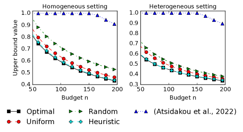
Figure 1: Upper bound value of our method instantiated with various weights compared to the upper bound of BayesElim (Atsidakou et al., 2022) in two settings.

3.2 PoE Bounds for Structured Bandits

Importantly, our analysis extends to the linear and hierarchical bandits in (2.2) and (2.3). Theorems 3.2 and 3.3 provide upper bounds on the PoE of $\texttt{PI-BAI}(\omega)$ in these settings. To the best of our knowledge, these are the first prior-dependent bounds for fixed-budget Bayesian BAI in these settings.

Theorem 3.2 (Upper bound for linear bandit).

Assume that $x_{i}\neq x_{j}$ for any $i\neq j$, and that there exists $S>0$ such that $\lVert x\rVert_{2}^{2}\leq S$ for any $x\in\mathcal{X}$. Then, for all $\omega\in\Delta^{+}_{K}$, the expected PoE of $\texttt{PI-BAI}(\omega)$ under the linear bandit problem (2.2) is upper bounded as

$$\mathcal{P}_{n} \leq\sum_{\begin{subarray}{c}i,j\in[K]\\ i\neq j\end{subarray}}\frac{e^{-\frac{(\mu_{0}^{\top}x_{i}-\mu_{0}^{\top}x_{j})^{2}}{2\lVert x_{i}-x_{j}\rVert^{2}_{\Sigma_{0}}}}}{\sqrt{1+\frac{c_{i,j}}{\lVert x_{i}-x_{j}\rVert^{2}_{\hat{\Sigma}_{n}}}}}\,,$$

where $c_{i,j}=\Omega(1)$, $\lambda_{1}(\hat{\Sigma}_{n})=\mathcal{O}(1/n)$, and they depend on both prior parameters and allocation weights. In particular, $\mathcal{P}_{n}=\mathcal{O}(1/\sqrt{n})$ and we recover Theorem 3.1 when $x_{i}=e_{i}\in^{K}$ and $\Sigma_{0}={\rm{diag}}(\sigma_{0,i}^{2})_{i\in[K]}$. Full expressions and proofs are given in Section C.3.

Similarly to our results in multi-armed bandits, $\mathcal{P}_{n}=\mathcal{O}(1/\sqrt{n})$ since $\lambda_{1}(\hat{\Sigma}_{n})=\mathcal{O}(1/n)$. Also, this bound captures the benefit of using informative priors. Indeed, $\mathcal{P}_{n}\to 0$ when the prior variances are small, i.e. $\Sigma_{0}\to 0_{L\times L}$, or when the prior gaps are large, $|\mu_{0}^{\top}x_{i}-\mu_{0}^{\top}x_{j}|\to\infty$.

Theorem 3.3 (Upper bound for hierarchical bandit).

For all $\omega\in\Delta^{+}_{K}$, the expected PoE of $\texttt{PI-BAI}(\omega)$ under the hierarchical bandit problem (2.3) is upper bounded as

$$\mathcal{P}_{n}\leq\sum_{\begin{subarray}{c}i,j\in[K]\\ i\neq j\end{subarray}}\frac{e^{-\frac{(\nu^{\top}b_{i}-\nu^{\top}b_{j})^{2}}{2(\|b_{i}-b_{j}\|_{\Sigma}^{2}+\sigma^{2}_{0,i}+\sigma^{2}_{0,j})}}}{\sqrt{1+\frac{c_{i,j}}{\hat{\sigma}_{n,i}+\hat{\sigma}_{n,j}}}}\,,$$

where $c_{ij}=\Omega(1)$ and $\hat{\sigma}^{2}_{n,i}=\Omega(1/n)$ and they all depend on both the prior parameters and allocation weights. In particular, $\mathcal{P}_{n}=\mathcal{O}(1/\sqrt{n})$. Full expressions and proofs are given in Section C.4.

The term $\|b_{i}-b_{j}\|_{\Sigma}^{2}+\sigma^{2}_{0,i}+\sigma^{2}_{0,j}$ accounts for the prior uncertainty of both arms and effects. If the effects are deterministic ($\Sigma\to 0_{L\times L}$) then our bound recovers the upper bound of MAB with prior mean $\mu_{0,i}=\nu^{\top}b_{i}$. On the other hand, if the arms are deterministic given the effects ($\sigma^{2}_{0,i}\to 0$), the bound only depends on the effect covariance. Finally, if the prior is informative by its gap ($|\nu^{\top}b_{i}-\nu^{\top}b_{j}|\to\infty\,$) or by its variance ($\Sigma\to 0_{L\times L}$ and $\sigma^{2}_{0,i}\to 0$), then $\mathcal{P}_{n}\to 0$.

3.3 Allocation Strategies

Instantiating our algorithm requires choosing the potentially prior-dependent allocation weights. Though our bound holds for any such choice, different principles can be used to find empirically satisfying allocations.

Allocation by optimization.

Our upper bounds on the PoE in Theorems 3.1, 3.2 and 3.3 are of the form

$$\mathcal{P}_{n}\leq C_{\rm{prior}}(\omega,n)\,,$$

where $C_{\rm{prior}}(\omega,n)=\mathcal{O}(1/\sqrt{n})$ depends on the prior and allocation weights $\omega$. Since it is valid for any $\omega\in\Delta^{+}_{K}$, we define the optimized allocation weights as

$$\omega^{\rm{opt}}=\operatorname*{argmin}_{w\in\Delta_{K}^{+}}C_{\rm{prior}}(\omega,n)\,.$$ (11)

We denote this variant $\texttt{PI-BAI}(\omega^{\rm{opt}})$. To fix ideas and give intuition, we give the explicit solution for MAB with $K=2$. By Theorem 3.1,

$$\mathcal{P}_{n}\leq\frac{e^{-\frac{(\mu_{0,1}-\mu_{0,2})^{2}}{2(\sigma^{2}_{0,1}+\sigma^{2}_{0,2})}}+e^{-\frac{(\mu_{0,1}-\mu_{0,2})^{2}}{2(\sigma^{2}_{0,1}+\sigma^{2}_{0,2})}}}{\sqrt{1+n\phi_{1,2}(\omega_{1},\omega_{2})}}\,,$$

which can be optimized to obtain

$$\omega^{\rm{opt}}_{1}=\Pi_{[0,1]}\Big{(}\frac{1}{2}-\frac{(\sigma^{2}_{0,2}-\sigma^{2}_{0,1})\sigma^{2}}{2n\sigma^{2}_{0,1}\sigma^{2}_{0,2}}\Big{)}\,,\qquad\omega^{\rm{opt}}_{2}=1-\omega^{\rm{opt}}_{1}\,,$$ (12)

where $\Pi_{[a,b]}(\cdot)$ is the projection on $[a,b]$. This expression gives much insight into the allocation strategy. First, in the case of equal prior confidence $\sigma^{2}_{0,1}=\sigma^{2}_{0,2}$, allocating the same amount of samples for each arm is optimal. On the other hand, if for example $\sigma^{2}_{0,1}\ll\sigma^{2}_{0,2}$ for small budget $n$, we would have $\omega^{\rm{opt}}_{2}\gg\omega^{\rm{opt}}_{1}$, and hence most of the budget would be allocated to the arm with high prior variance (low initial confidence). This discussion is only valid for small budgets: as $n\to+\infty$, the optimal choice is to divide the budget equally between both arms, since the prior relevance vanishes asymptotically. On the other hand, a saturation phenomenon happens for ‘too small’ budgets: if $n<2\sigma^{2}\left|\frac{\sigma_{0,2}^{2}}{\sigma_{0,1}^{2}}-\frac{\sigma_{0,1}^{2}}{\sigma_{0,2}^{2}}\right|$, the weight of the arm with larger prior variance is equal to 1 due to the projection. Note that (12) does not depend on the prior gap $\Delta_{0}$, which is coherent since identifying the optimal arm is strictly equivalent to identifying the worst arm when dealing with 2 arms. However, this is not necessarily the case when $K$ is larger, as discussed in Section D.8.

Since the objective function in (11) is non-convex for $K>2$, we use numerical optimization to solve it (e.g. L-BFGS-B (Virtanen et al., 2020)). Thankfully, this optimization is done just once before interacting with the environment. These optimized weights remain non-guaranteed to be good, because (11) is only optimal with respect to the bound we derived. We found it useful in practice to mix them with the heuristic weight $\omega^{\texttt{h}}$ defined in Section 3.1. This allocation is motivated by having a small probability of error when plugged in the bound (Figure 1), and our theoretical guarantees (Theorem 3.1) still hold because the weights are a function of the prior. Hence, we define the new optimized weight as $\alpha\omega^{\rm{opt}}_{i}+(1-\alpha)\frac{\mu_{0,i}\sigma_{0,i}}{\sum_{k\in[K]}\mu_{0,k}\sigma_{0,k}}$. For simplicity, we also refer this as $\omega^{\rm{opt}}$. We tested the value of the parameter $\alpha$ in various settings, and found that it is generally around 0.5 (Section D.7).

Allocation by optimal design.

In the linear bandit setting, we generalize ideas from optimal experimental design (Lattimore and Szepesvári, 2020, Chapter 21) to Bayesian MAB, linear and hierarchical bandits. To the best of our knowledge, our work is the first to exploit this idea for such settings. Finding an (approximate) Bayesian G-optimal design (see e.g. López-Fidalgo (2023, Chapter 4) for a review) is equivalent to maximizing the log-determinant of the regularized information matrix defined as

$$\omega^{\rm{G\shortminus opt}}=\operatorname*{argmax}_{\omega\in\Delta_{K}^{+}}\log\det\big{(}n\sigma^{-2}\sum_{k\in[K]}\omega_{k}x_{k}x_{k}^{\top}+\Sigma_{0}^{-1}\big{)}\,.$$

This leads to budget allocations that minimize the worst-case posterior variance in all directions. We quantify the effects of using such an allocation in the upper bound:

Corollary 3.4 (Upper bound of $\texttt{PI-BAI}(\omega^{\rm{G\shortminus opt}})$).

Assume that $x_{i}\neq x_{j}$ for any $i\neq j$, and that there exists $S>0$ such that $\lVert x\rVert_{2}^{2}\leq S$ for any $x\in\mathcal{X}$. The expected PoE of $\texttt{PI-BAI}(\omega^{\rm{G\shortminus opt}})$ in the linear bandit problem (2.2) with diagonal covariance matrix $\Sigma_{0}$ is upper bounded as

$$\mathcal{P}_{n}\leq\sum_{\begin{subarray}{c}i,j\in[K]\\ i\neq j\end{subarray}}\frac{e^{-\frac{(\mu_{0}^{\top}x_{i}-\mu_{0}^{\top}x_{j})^{2}}{2\lVert x_{i}-x_{j}\rVert^{2}_{\Sigma_{0}}}}}{\sqrt{1+\frac{n}{2d\sigma^{2}}c_{i,j}}}\,,$$

where $c_{i,j}=\Omega(1)$. The full expressions and proofs are given in Section C.3. The result also holds for the MAB setting when $x_{i}=e_{i}\in^{K}$ and $\Sigma_{0}={\rm{diag}}(\sigma_{0,i}^{2})_{i\in[K]}$, and for the hierarchical setting with the equivalent model (2.3) when $\Sigma$ is diagonal.

G-optimal design can be applied for MAB, by using $x_{i}=e_{i}$ for any $i\in[K]$ and $\Sigma_{0}={\rm{diag}}(\sigma_{0,i}^{2})_{i\in[K]}$, and also for hierarchical bandits by using its connection to the linear model (2.3).

Note that both allocation weights $\omega^{\rm{opt}}$ and $\omega^{\rm{G\shortminus opt}}$ are prior-dependent but not instance-dependent. In particular, they enjoy the theoretical guarantees we derived in Section 4.

Allocation by warm-up.

Finally, we present an adaptive allocation rule, for which our theoretical results do not apply directly, but performs well in practice. Here we use a warm-up policy $\pi_{\rm{w}}$ to interact with the bandit environment for $n_{\rm{w}}$ rounds (the warm-up phase), and then choose some allocation weights $\omega_{\pi_{\rm{w}}}$ based on the prior and the data collected through the interaction. The warm-up policy can be any decision-making policy that (preferably) takes as input the prior distribution. Motivated by its good performance in BAI (Lee et al., 2023), we choose $\pi_{\rm{w}}$ to be Thompson sampling, and select the allocation weights to be proportional to the number of pulls to each arm during the warm-up phase:

$$\omega^{\rm{TS}}_{i} =\frac{\sum_{t\in[n_{\rm{w}}]}\mathds{1}\!\left\{A_{t}=i\right\}}{n_{\rm{w}}}\,, \forall i\in[K]\,.$$ (13)

To illustrate the differences between optimized weights ($\texttt{PI-BAI}(\omega^{\rm{opt}})$) and learned weights with Thompson sampling as a warm-up policy ($\texttt{PI-BAI}(\omega^{\rm{TS}})$), we return to our motivating example in Section 3.1, where $K=3$, $\mu_{0}=(1,1.9,2)$ and $\sigma_{0,i}=0.3$ for all $i\in[3]$. We set the budget as $n=100$. We repeat $10^{4}$ times the following experiment: we sample a bandit instance from the prior and run Thompson sampling for $n_{\rm{w}}=20$ rounds, then construct the allocation weights $\omega^{\rm{TS}}$. Computing the weights $\omega^{\rm{opt}}$ by numerical optimization of (11) is done once at the beginning of these experiments.

Figure 2 shows an empirical comparison of the weights on 2 problem instances and on average over $10^{4}$ runs. We see that, in this example, both allocation strategies assign high weights to arms 2 and 3, while allocating a small weight to arm 1. This is because, based on the prior information, arm 1 is highly unlikely to be the optimal arm. Then, the primary objective revolves around selecting the optimal arm among arms 2 and 3. Also, while the allocation weights $\omega^{\textsc{ts}}_{i}$ vary with each bandit instance, their average values in all instances are similar to those of $\omega^{\rm{opt}}_{i}$. Thus $\texttt{PI-BAI}(\omega^{\rm{TS}})$ is more adaptive than $\texttt{PI-BAI}(\omega^{\rm{opt}})$, while both have similar average behavior.

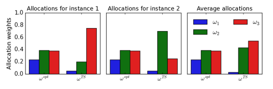
Figure 2: Allocations weights $\omega^{\rm{opt}}_{i}$ and $\omega^{\rm{TS}}_{i}$.

4 General Proof Scheme

We outline the key technical insights to derive our Bayesian proofs. The idea is general and can be applied to all our settings. Specific proofs for these settings are in Appendix C.

From Frequentist to Bayesian proof.

To analyze their algorithm in the MAB setting, Atsidakou et al. (2022) rely on the strong restriction that $\sigma_{0,i}=\sigma_{0}$ for all arms $i\in[K]$ and tune their allocations as a function of the noise variance $\sigma^{2}$ such that in the Gaussian setting, the posterior variances $\hat{\sigma}_{n,i}^{2}$ in (3) are equal for all arms $i\in[K]$. This assumption is needed to directly leverage results from Karnin et al. (2013), thus allowing them to bound the frequentist PoE $\mathbb{P}\big{(}J_{n}\neq i_{*}(\theta)\mid\theta\big{)}\leq B(\theta)$ for a fixed instance $\theta$. Then, the expected PoE, $\mathcal{P}_{n}=\mathbb{E}\left[\mathbb{P}\big{(}J_{n}\neq i_{*}(\theta)\mid\theta\big{)}\right]$, is bounded by computing $\mathbb{E}_{\theta\sim P_{0}}\left[B(\theta)\right]$. We believe it is not possible to extend such technique for general choices of allocations $n_{i}$ and prior variances $\sigma^{2}_{0,i}$. Thus, we pursue an alternative approach, establishing the result in a fully Bayesian fashion. We start with a key observation.

Key reformulation of the expected PoE.

We observe that the expected PoE can be reformulated as follows

$$\mathcal{P}_{n} =\mathbb{E}\left[\mathbb{P}\big{(}J_{n}\neq i_{*}(\theta)\mid\theta\big{)}\right]=\mathbb{E}\left[\mathbb{P}\big{(}J_{n}\neq i_{*}(\theta)\mid H_{n}\big{)}\right].$$

This swap of measures means that to bound $\mathcal{P}_{n}$, we no longer bound the probability of

$$J_{n}=\operatorname*{argmax}_{i\in[K]}\mathbb{E}\left[r(i;\theta)\,|\,H_{n}\right]\neq\operatorname*{argmax}_{i\in[K]}r(i;\theta)=i_{*}(\theta)$$

for any fixed $\theta$. Instead, we only need to bound that probability when $\theta$ is drawn from the posterior distribution. Precisely, we bound the probability that the arm $i$ maximizing the posterior mean $\mathbb{E}\left[r(i;\theta)\mid H_{n}\right]$ differs from the arm $i$ maximizing the posterior sample $r(i;\theta)\mid H_{n}$. This is achieved by first noticing that $\mathcal{P}_{n}$ can be rewritten as

$$\mathcal{P}_{n}=\sum_{\begin{subarray}{c}i,j\in[K]\\ i\neq j\end{subarray}}\mathbb{E}\left[\mathbb{P}\left(i_{*}(\theta)=i\mid J_{n}=j,H_{n}\right)\mathds{1}\!\left\{J_{n}=j\right\}\right].$$

The rest of the proof consists of bounding the above conditional probabilities for distincts $i$ and $j$, and this depends on the setting (MAB, linear or hierarchical). Roughly speaking, this is achieved as follows. $\mathbb{P}\left(i_{*}(\theta)=i\mid H_{n},J_{n}=j\right)$ is the probability that arm $i$ maximizes the posterior sample $r(\cdot;\theta)$, given that arm $j$ maximizes the posterior mean $\mathbb{E}\left[r(\cdot;\theta)\mid H_{n}\right]$. We show that this probability decays exponentially with the squared difference $(\mathbb{E}\left[r(i;\theta)\,|\,H_{n}\right]-\mathbb{E}\left[r(j;\theta)\,|\,H_{n}\right])^{2}$. Taking the expectation of this term under the history $H_{n}$ gives the desired $\mathcal{O}(1/\sqrt{n})$ rate. All technical details and full explanations can be found in Appendix C. This proof introduces a novel perspective for Bayesian BAI, distinguished by its tighter prior-dependent bounds on the expected PoE and ease of extension to more complex settings like linear and hierarchical bandits. However, its application to adaptive algorithms could be challenging, particularly due to the complexity of taking expectations under the history $H_{n}$ in that case. Also, extending this proof to non-Gaussian distributions is an interesting direction for future work. Note that PI-BAI is applicable beyond the Gaussian case, as done in Sections A.2 and D.2 featuring an approximate approach to logistic bandits (Chapelle and Li, 2012).

5 Experiments

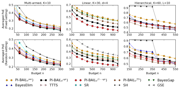
Figure 3: Averaged PoE with varying budgets for the Fixed and Random settings. We compare PI-BAI instantiated with different allocations strategies to the baselines BayesElim, TTTS, SR, SH in multi-armed and hierarchical bandits, and to BayesGap and GSE in linear bandits.

We conduct several experiments to evaluate the performance of PI-BAI. In all experiments, we set the observation noise to $\sigma=1$ and run algorithms $10^{4}$ times and display the (narrow) standard error. The code is available in the supplementary material, and additional experiments and details are presented in Section D.1. We consider four variants of $\texttt{PI-BAI}(\omega)$ varying in allocation weights: $\texttt{PI-BAI}(\omega^{\rm{uni}})$ (uniform weights), $\texttt{PI-BAI}(\omega^{\rm{opt}})$ (optimized weights with mixing), $\texttt{PI-BAI}(\omega^{\rm{G\shortminus opt}})$ (G-optimal design) and $\texttt{PI-BAI}(\omega^{\rm{TS}})$ (warmed-up with Thompson Sampling). The question of tuning the warm-up length $n_{\rm{w}}$ is discussed in Section D.7 and we set $n_{\rm{w}}=K$.

Multi-armed bandit.

We consider two settings, Fixed and Random. For both, we set $K=10$ and $\sigma_{0,i}$ evenly spaced between $0.1$ and $0.5$. In the Fixed setting, $\mu_{0,i}$ is evenly spaced between $0$ and $1$ whereas in the Random one, $\mu_{0,i}\sim\mathcal{U}([0,1])$. We compare PI-BAI variants to state-of-the-art Bayesian methods, top-two Thompson sampling (TTTS) (Russo, 2016; Jourdan et al., 2022) and BayesElim (Atsidakou et al., 2022), as well as to frequentist elimination algorithms: successive rejects (SR) (Audibert et al., 2010) and sequential halving (SH) (Karnin et al., 2013). Note that TTTS does not come with theoretical guarantees in the fixed-budget setting, but we include it given its good empirical performance.

Linear bandit.

We let $d=4$ and $K=30$. Then we construct the arm set $\mathcal{X}$ by sampling arms $x_{i}$ from a multivariate Gaussian distribution with mean $0_{d}$ and covariance $I_{d}$. In the Fixed setting, the prior mean is flat $\mu_{0}=(1,\dots,1)$ whereas in the Random setting, the prior means are sampled uniformly from $[0,1]$ as $\mu_{0,i}\sim\mathcal{U}([0,1])$. For both settings, $\Sigma_{0}={\rm diag}(\sigma_{0,i}^{2})_{i\in[K]}$ where the $\sigma_{0,i}$’s are evenly spaced between $0.1$ and $0.5$. We compare our methods with two algorithms that were designed for linear bandits; BayesGap (Hoffman et al., 2014) and GSE (Azizi et al., 2021), the current (tractable) state-of-the-art that leverages G-optimal design to perform successive elimination. Other methods that leverage the same elimination idea and have lower performances on these settings (Alieva et al., 2021; Yang and Tan, 2022) are not tested.

Hierarchical bandit.

Here, each mixing weight $b_{i}$ is chosen uniformly between 0 and 1, and then normalized to form a probability vector. In the Fixed setting, The $\nu_{i}$’s are evenly spaced in $[-1,1]$, whereas each $\nu_{i}\sim\mathcal{U}([-1,1])$ in the Random setting. In both settings, $\Sigma$ is diagonal with entries evenly spaced in $[0.1^{2},0.5^{2}]$, and $\Sigma_{0}$ is also diagonal, where the $\sigma_{0,i}$’s are evenly spaced between $0.1$ and $0.5$. The prior distribution for all Bayesian algorithms (except PI-BAI) is simply obtained by marginalizing out the effects. This allows obtaining $\mu_{0,i}$ and $\sigma_{0,i}$, even for algorithms that are not suitable for hierarchical priors. Though there is no explicit baseline for this setting, we implement TS based on meTS (Aouali et al., 2023) and we compare with frequentist and Bayesian elimination strategies agnostic to the structure. Despite the connection to linear bandits, we do not include such baselines as they do not perform well due to their inefficient representation of the structure.

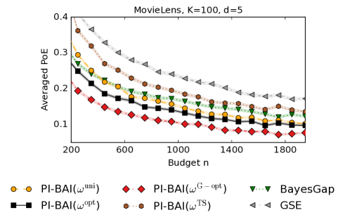
Figure 4: Averaged PoE on MovieLens.

Results on simulated data (Figure 3).

Overall, despite setting-dependent variations, $\texttt{PI-BAI}(\omega^{\rm{G\shortminus opt}})$ is the best-performing version, closely followed by $\omega^{\rm{opt}}$. In the hierarchical experiments $\texttt{PI-BAI}(\omega^{\rm{TS}})$ surpasses all baselines, highlighting the effectiveness of this method in capturing the underlying problem structure. These observations reaffirm that leveraging prior information is a powerful and practical tool to scale the applicability of BAI to cases with a large number of arms in limited data regimes.

MovieLens data experiment (Figure 4).

The MovieLens (Lam and Herlocker, 2016) dataset is a large sparse matrix of ratings from 6040 users (rows) on movies (columns, we subsampled $K=100$). We first perform a low-rank matrix factorization to obtain $d=5$ dimensional vectors representing users (context) and movies (actions) as well as estimated corresponding values. We then simulate an online interaction setting: at each round $t\in[n]$, a user vector is picked uniformly at random and a movie is chosen by the policy, leading to a reward $Y_{t}\sim\mathcal{N}(x_{t}^{\top}\theta_{t},\sigma^{2})$. This semi-synthetic problem allows us to assess PI-BAI’s robustness to prior misspecification since the bandit instances are no longer sampled from the prior. More details in Section D.1.

6 Conclusion

We revisit the Bayesian fixed-budget BAI for PoE minimization (Atsidakou et al., 2022) and propose a simple yet efficient algorithm for MAB, linear and hierarchical bandits. Our new proof technique reveals a flexible and smaller upper bound on the expected PoE. In particular, this allows us to derive the first prior-dependent Bayesian PoE upper bounds for linear and hierarchical bandits. We believe that our work sheds a new light on the adaptativity-vs-generality trade-off in BAI algorithm design while opening several avenues for future research. Our work relies on the assumption that the algorithm has access to the true instance-generating distribution, i.e. the prior. Though this assumption is very common in the Bayesian bandits literature, it is unrealistic in many scenarios. An interesting question for future work is to explore methods to learn the generative distribution and the related consequences of prior misspecification on the expected PoE of PI-BAI (Kveton et al., 2021; Simchowitz et al., 2021; Nguyen and Vernade, 2023).

Broader Impact Statement

In this work we have developed and analyzed generic algorithms for certain optimization problems. Employing our methods may lead to savings in computation and energy. Since our problem setting and our algorithms are generic, the broader (social) impact is unforeseeable and depends on the area where the methods are applied.

Organization of the Appendix

The supplementary material is organized as follows. In Appendix A, we provide additional general additional remarks. In Appendix B, we mention additional existing works relevant to our work. In Appendix C, we give complete statements and proofs of our theoretical results. In Appendix D, we provide additional numerical experiments.

Appendix A Additional Discussions

A.1 Motivating examples for hierarchical bandits

In this section, we discuss motivating examples for using hierarchical models in pure exploration settings.

Hyper-parameter tuning.

Here the goal is to find the best configuration for a neural network using $n$ epochs (Li et al., 2017). A configuration $i$ is represented by a scalar $\theta_{i}\in$ which quantifies the expected performance of a neural network with such configuration. Again, it is intuitive to learn all $\theta_{i}$ individually. Roughly speaking, this means running each configuration for $\lfloor\frac{n}{K}\rfloor$ epochs and selecting the one with the highest performance. This is statistically inefficient since the number of configurations can be combinatorially large. Fortunately, we can leverage the fact that configurations often share the values of many hyper-parameters. Precisely, a configuration is a combination of multiple hyper-parameters, each set to a specific value. Then we represent each hyper-parameter $\ell\in[L]$ by a scalar parameter $\mu_{\ell}\in$, and the configuration parameter $\theta_{i}$ is a mixture of its hyper-parameters $\mu_{\ell}$ weighted by their values. That is, $\theta_{i}=\sum_{\ell\in[L]}b_{i,\ell}\mu_{\ell}+\epsilon_{i}$, where $b_{i,\ell}$ is the value of hyper-parameter $\ell$ in configuration $i$ and $\epsilon_{i}$ is a random noise to incorporate uncertainty due to model misspecification.

Drug design.

In clinical trials, $K$ drugs are administrated to $n$ subjects, with the goal of finding the optimal drug design. Each drug is parameterized by its expected efficiency $\theta_{i}\in\mathbb{R}$. As in the previous example, it is intuitive to learn each $\theta_{i}$ individually by assigning a drug to $\lceil\frac{n}{K}\rceil$ subjects. However, this is inefficient when $K$ is large. We leverage the idea that drugs often share the same components: each drug parameter $\theta_{i}$ is a combination of component parameters $\mu_{l}$, each accounting for a specific dosage. More precisely, the parameter of drug $i$ can be modeled as $\theta_{i}=\sum_{l\in[L]}b_{i,l}\mu_{l}+\epsilon_{i}$ where $\epsilon_{i}$ accounts for uncertainty due to model misspecification. Similarly to the hyper-parameter tuning example, this models correlations between drugs and it can be leveraged for more efficient use of the whole budget of $n$ epochs.

A.2 Beyond Gaussian distributions

The standard linear model (2.2) can be generalized beyond linear mean rewards. The Generalized Linear Bandit (GLB) model with prior $P_{0}$ writes (Filippi et al., 2010; Kveton et al., 2020)

$$\theta\sim P_{0}$$ (14)

$$Y_{t}\mid\theta,A_{t}\sim P(.;\theta,A_{t})\quad\forall t\in[n]\,,$$

where the reward distribution $P(.;\theta,A_{t})$ belongs to some exponential family with mean reward $r(A_{t};\theta)=\phi(\theta^{\top}x_{A_{t}})$. $\phi$ is called the link function. The log-likelihood of such reward distribution can be written

$$\mathcal{L}_{n}(\theta)=\sum_{t=1}^{n}\log\mathrm{P}(Y_{t};\theta,A_{i})=\sum_{t=1}^{n}Y_{t}\theta^{\top}x_{A_{t}}-A(\theta^{\top}x_{A_{t}})+h(Y_{t})\,,$$

where $A$ is a log-partition function and $h$ another function. Importantly, (14) encompasses the logistic bandit model with the particular link function $\phi(z)=\frac{1}{1+e^{-z}}$.

The main challenge of (14) is that closed-form posterior generally does not exist. One method is to approximate the posterior distribution of $\theta$ given $H_{n}$ with Laplace approximation: $\mathbb{P}(\theta\mid H_{n})$ is approximated with a multivariate Gaussian distribution with mean $\hat{\theta}_{\mathrm{MAP}}$ and covariance $\hat{\Sigma}_{\mathrm{Lap}}$, where $\hat{\theta}_{\mathrm{MAP}}$ is the maximum a posteriori,

$$\hat{\theta}_{\mathrm{MAP}}=\operatorname*{argmax}_{\theta}\mathcal{L}_{n}(\theta)P_{0}(\theta)$$

$$\hat{\Sigma}^{-1}_{\mathrm{Lap}}=\sum_{t=1}^{n}\dot{\phi}(\hat{\theta}_{\mathrm{MAP}}^{\top}x_{A_{t}})x_{A_{t}}x_{A_{t}}^{\top}\,,$$

where $\phi$ is assumed continuously differentiable and increasing. Note that $\hat{\theta}_{\mathrm{MAP}}$ can be computed efficiently by iteratively reweighted least squares (Wolke and Schwetlick, 1988).

Logistic Bandit.

In the particular case where the reward distribution is Bernoulli, the model writes

$$\theta \sim\mathcal{N}(\mu_{0},\Sigma_{0})$$

$$Y_{t}\mid\theta,A_{t} \sim\mathcal{B}(\phi(\theta^{\top}x_{A_{t}})) \forall t\in[n]\,,$$ (15)

where $\phi$ is the logistic function. Then the mean posterior reward can be approximated as

$$\mathbb{E}_{\theta\sim\mathcal{N}(\hat{\theta}_{\mathrm{MAP}},\hat{\Sigma}_{\mathrm{Lap}})}\left[\phi(\theta^{\top}x_{i})\right]\approx\frac{\phi(\hat{\theta}_{\mathrm{MAP}}^{\top}x_{i})}{\sqrt{1+\frac{\pi}{8}\|x_{i}\|_{\hat{\Sigma}_{\mathrm{Lap}}}}}\,,$$

and the decision after $n$ rounds is $J_{n}=\operatorname*{argmax}_{i\in[K]}\frac{\phi(\hat{\theta}_{\mathrm{MAP}}^{\top}x_{i})}{\sqrt{1+\frac{\pi}{8}\|x_{i}\|_{\hat{\Sigma}_{\mathrm{Lap}}}}}\,$.

Proving an upper bound on the expected PoE of this algorithm is challenging. Particularly, upper bounding the expectation with respect to $H_{n}$ is hard because one needs to show that $\hat{\theta}_{\mathrm{MAP}}$ concentrates in norm towards its expectation $\mathbb{E}_{H_{n}}\left[\hat{\theta}_{\mathrm{MAP}}\right]$. We leave this study for future work. However, we provide numerical experiments for this setting in Section D.2.

A.3 Additional Remarks on Hierarchical Models

The two-level prior we consider has a shared latent parameter $\mu=(\mu_{\ell})_{\ell\in[L]}\in^{L}$ representing $L$ effects impacting each of the $K$ arm means:

$$\mu \sim Q$$

$$\theta_{i} \sim P_{0,i}(\cdot;\mu) \forall i\in[K]$$

$$Y_{t}\mid\mu,\theta,A_{t} \sim P(\cdot;\theta_{A_{t}}) \forall t\in[n]\,,$$

where $Q$ is the latent prior on $\mu\in^{L}$.

In the Gaussian setting (2.3), the maximum likelihood estimate of the reward mean of action $i$, $B_{n,i}/n_{i}$, contributes to (7) proportionally to its precision $n_{i}/(n_{i}\sigma^{2}_{0,i}+\sigma^{2})$ and is weighted by its mixing weight $b_{i}$. (8) is a standard Gaussian posterior, and (9) takes into account the information of the conditional posterior. Finally, (9) takes into account the arm correlation through its dependence on $\hat{\sigma}_{n,i}$ and $\hat{\mu}_{n,i}$. While the properties of conjugate priors are useful for inference, other models could be considered with approximate inference techniques (Urteaga and Wiggins, 2018; Phan et al., 2019).

Link with linear bandit (cont.).

The slightly unusual characteristic of (2.3) is that the prior distribution has correlated components. This can be addressed by the whitening trick (Bishop, 2006), defining $\tilde{\mu}=\bar{\Sigma}^{-1/2}\bar{\mu}$ and $\tilde{b}_{i}=\bar{\Sigma}^{1/2}\bar{b}_{i}$, giving

$$\tilde{\mu} \sim\mathcal{N}(\bar{\Sigma}^{-1/2}\bar{\nu},I_{L+K})$$

$$Y_{t}\mid\tilde{\mu},A_{t} \sim\mathcal{N}(\tilde{b}^{\top}_{A_{t}}\tilde{\mu},\sigma^{2}) \forall t\in[n]\,,$$ (16)

where $I_{L+K}$ is the $(L+K)$-dimensional identity matrix. Then, (A.3) corresponds to a linear bandit model with $K$ arms and $d=K+L$ features. However, this model comes with some limitations. First, when computing posteriors under (A.3), the time and space complexities are $\mathcal{O}((K+L)^{3})$ and $\mathcal{O}((K+L)^{2})$ respectively, compared to the $\mathcal{O}(K+L^{3})$ and $\mathcal{O}(K+L^{2})$ for our model (9). The feature dimension $d=K+L$ can be reduced to $d=K$ through the following QR decomposition: $\tilde{B}=\big{(}\tilde{b}_{1},\dots,\tilde{b}_{K}\big{)}\in\mathbb{R}^{(K+L)\times K}$ can be expressed as $\tilde{B}=VR$, where $V\in\mathbb{R}^{(K+L)\times K}$ is an orthogonal matrix and $R\in\mathbb{R}^{K\times K}$. This leads to the following model $\check{\mu}\sim\mathcal{N}(V^{\top}\bar{\Sigma}^{-1/2}\bar{\nu},V^{\top}V)$ and $Y_{t}\mid\check{\mu},A_{t}\sim\mathcal{N}(R^{\top}_{A_{t}}\check{\mu},\sigma^{2})$, yet the feature dimension $d$ remains at the order of $K$, and computational efficiency is not improved with respect to $K$.

From hierarchical bandit to MAB.

Marginilizing the hyper-prior in (2.3) leads to a MAB model,

$$\theta_{i} \sim\mathcal{N}(b_{i}^{\top}\nu,\sigma^{2}_{0,i}+b_{i}^{\top}\Sigma b_{i}) \forall i\in[K]$$ (17)

$$Y_{t}\mid\mu,\theta,A_{t} \sim\mathcal{N}(\theta_{A_{t}},\sigma^{2}) \forall t\in[n]\,.$$ (18)

In this marginalized model, the agent does not know $\mu$ and he doesn’t want to model it. Therefore, only $\theta$ is learned. The marginalized prior variance $\sigma^{2}_{0,i}+b_{i}^{\top}\Sigma b_{i}$ accounts for the uncertainty of the not-modeled effects.

Appendix B Extended Related Work

In this section, we provide additional references relevant to our work.

Bayesian bandits in structured environments.

Bayesian bandits algorithms under hierarchical models have been heavily studied (Hong et al., 2020; Kveton et al., 2021; Basu et al., 2021; Hong et al., 2022a, b; Peleg et al., 2022; Aouali et al., 2023; Aouali, 2023). All the aforementioned papers propose methods to explore efficiently in the structured environment to minimize the (Bayesian) regret. The hierarchical model we use is derived from Aouali et al. (2023). Beyond regret minimization, Bayesian structured models also found success in simple regret minimization (Azizi et al., 2023) and off-policy learning in bandits (Hong et al., 2023).

Bayesian simple regret minimization.

Azizi et al. (2023) considers the problem of simple regret minimization in a Bayesian hierarchical setting. Their algorithm is based on Thompson sampling, and choose an arm at the last round by sampling according to the number of pulls. This leads to a $\mathcal{O}(1/\sqrt{n})$ rate on the Bayesian simple regret. Recently, Komiyama et al. (2023) derived a method for Bayesian simple regret minimization that asymptotically matches their proposed lower bound scaling in $\mathcal{O}(1/n)$. Their result does not contradict our analysis because as mentioned in their work, the difference between the simple regret and PoE matters in terms of rate when considering a Bayesian objective, unlike in the frequentist case. Moreover, their method is designed for Bernoulli rewards, and their algorithm does not use the prior distribution.

Appendix C Proofs

In this section, we give complete proof of our theoretical results. In Section C.1, we give proofs for the Bayesian posterior derivations and we provide technical results. In Section C.2, we prove Theorem 3.1. The proofs for linear bandits (Theorems 3.2 and 3.4) are given in Section C.3. In Section C.4, we provide proofs and technical remarks for hierarchical bandits (Theorem 3.3).

C.1 Technical Proofs and Posteriors Derivations

Bayesian computations.

We focus on the hierarchical Gaussian case (2.3) and detail the computations of posterior distributions. We first recall the model,

$$\mu \sim\mathcal{N}(\nu,\Sigma)$$

$$\theta_{i} \sim\mathcal{N}(b_{i}^{\top}\mu,\sigma_{0,i}^{2}) \forall i\in[K]$$

$$Y_{t}\mid\mu,\theta,A_{t} \sim\mathcal{N}(\theta_{A_{t}},\sigma^{2}) \forall t\in[n]\,,$$

where we recall that $B_{n,i}=\sum_{t\in\mathcal{T}_{i}}Y_{t}$ and $\mathcal{T}_{i}=\{t\in[n],\,A_{t}=i\}$.

Lemma C.1 (Gaussian posterior update).

For any $\rho\in\mathbb{R},\mu\in\mathbb{R}^{L},b\in\mathbb{R}^{L}$ and $\sigma,\sigma_{0}>0,m\in\mathbb{N}$, we have

$$\int_{\rho}\prod_{t\in[m]}\mathcal{N}\left(Y_{t};\rho,\sigma^{2}\right)\mathcal{N}\left(\rho;b^{\top}\mu,\sigma^{2}_{0}\right)\mathrm{d}\rho\propto\mathcal{N}\left(\mu;\mu_{m},\Sigma_{m}\right)\,,$$

with

$$\Sigma_{m}=\frac{m}{m\sigma^{2}_{0}+\sigma^{2}}bb^{\top};\quad\mu_{m}=\Sigma_{m}^{-1}\frac{\sum_{t\in[m]}Y_{t}}{m\sigma^{2}_{0}+\sigma^{2}}b\,.$$

Proof of Lemma C.1.

By keeping only terms that depend on $\mu$,

$$f(\mu) =\int_{\rho}\prod_{t\in[m]}\mathcal{N}\left(Y_{t};\rho,\sigma^{2}\right)\mathcal{N}\left(\rho;b^{\top}\mu,\sigma^{2}_{0}\right)\mathrm{d}\rho$$

$$\propto\int_{\rho}\exp\left\{-\frac{1}{2\sigma^{2}}\sum_{t\in[m]}(Y_{t}-\rho)^{2}-\frac{1}{2\sigma^{2}_{0}}(\rho-b^{\top}\mu)^{2}\right\}\mathrm{d}\rho$$

$$\propto\int_{\rho}\exp\left\{-\frac{1}{2}\rho^{2}\left(\frac{1}{\sigma^{2}_{0}}+\frac{m}{\sigma^{2}}\right)-2\rho\left(\frac{\sum_{t\in[m]}}{\sigma^{2}}+\frac{b^{\top}\mu}{\sigma^{2}_{0}}\right)\right\}\mathrm{d}\rho\exp\left\{-\frac{1}{2\sigma^{2}_{0}}\mu^{T}bb^{\top}\mu\right\}$$

$$\propto\exp\left\{\frac{1}{2}\left(\frac{1}{\sigma^{2}}\sum_{t\in[m]}Y_{t}+\frac{b^{\top}\mu}{\sigma^{2}_{0}}\right)^{2}\frac{\sigma^{2}_{0}\sigma^{2}}{\sigma^{2}+m\sigma^{2}_{0}}-\frac{1}{2\sigma^{2}_{0}}\mu^{T}bb^{\top}\mu\right\}$$

$$\propto\exp\left\{\frac{\sum_{t\in[m]}Y_{t}b^{\top}\mu}{\sigma^{2}+m\sigma^{2}_{0}}+\frac{\sigma^{2}}{2(\sigma^{2}+m\sigma^{2}_{0})}\mu^{\top}bb^{\top}\mu-\frac{1}{\sigma^{2}_{0}}bb^{\top}\right\}$$

$$\propto\exp\left\{-\frac{1}{2}\left(\mu^{\top}\frac{m}{\sigma^{2}+m\sigma^{2}_{0}}bb^{\top}\mu-2\mu^{\top}\frac{\sum_{t\in[m]}Y_{t}}{\sigma^{2}+m\sigma^{2}_{0}}b\right)\right\}$$

$$\propto\mathcal{N}\left(\mu;\mu_{m},\Sigma_{m}\right)\,.$$

∎

Lemma C.2 (Joint effect posterior).

For any $n\in[N]$, the joint effect posterior is a multivariate Gaussian $Q_{n}(\mu)=\mathcal{N}\left(\breve{\mu},\breve{\Sigma}_{n}\right)$, where

$$\breve{\Sigma}_{n}^{-1}=\Sigma^{-1}+\sum_{i\in[K]}\frac{n_{i}}{n_{i}\sigma_{0,i}^{2}+\sigma^{2}}b_{i}b_{i}^{\top},\quad\breve{\mu}_{n}=\breve{\Sigma}_{n}\Big{(}\Sigma^{-1}\nu+\sum_{i\in[K]}\frac{B_{n,i}}{n_{i}\sigma_{0,i}^{2}+\sigma^{2}}b_{i}\Big{)}\,.$$

Proof of Lemma C.2.

The joint effect posterior can be written as

$$Q_{n}(\mu) \propto\int_{\theta}\mathcal{L}_{\theta}\left(Y_{A_{1}},...,Y_{A_{n}}\right)P_{0}(\theta\mid\mu)\mathrm{d}\theta Q(\mu)$$

$$=\prod_{i\in[K]}\int_{\theta_{i}}\prod_{t\in\mathcal{T}_{i}}\mathcal{N}\left(Y_{t};\theta_{i},\sigma^{2}\right)\mathcal{N}\left(\theta_{i};b_{i}^{\top}\mu,\sigma^{2}_{0,i}\right)\mathrm{d}\theta_{i}\mathcal{N}\left(\mu;\nu,\Sigma\right)\,.$$

Applying Lemma C.1 gives

$$\int_{\theta_{i}}\prod_{t\in\mathcal{T}_{i}}\mathcal{N}\left(Y_{t};\theta_{i},\sigma^{2}\right)\mathcal{N}\left(\theta_{i};b_{i}^{\top}\mu,\sigma^{2}_{0,i}\right)\mathrm{d}\theta_{i} \propto\mathcal{N}\left(\mu;\bar{\mu}_{n,i},\bar{\Sigma}_{n,i}\right)\,,$$

with

$$\breve{\Sigma}_{n,i}^{-1}=\frac{n_{i}}{\sigma^{2}_{0,i}n_{i}+\sigma^{2}}b_{i}b_{i}^{\top},\qquad\breve{\mu}_{n,i}=\breve{\Sigma}_{n,i}b_{i}\frac{n_{i}}{\sigma^{2}_{0,i}n_{i}+\sigma^{2}}\frac{B_{n,i}}{n_{i}}\,.$$

Therefore, the joint effect posterior is a product of Gaussian distributions,

$$Q_{n}(\mu)\propto\prod_{i\in[K]}\mathcal{N}\left(\mu;\breve{\mu}_{n,i},\breve{\Sigma}_{n,i}\right)\mathcal{N}\left(\mu;\nu,\Sigma\right)\propto\mathcal{N}\left(\mu;\breve{\mu}_{n},\breve{\Sigma}_{n}\right)\,,$$

where

$$\breve{\Sigma}_{n} =\Sigma^{-1}+\sum_{i\in[K]}\breve{\Sigma}_{n,i}=\Sigma^{-1}+\sum_{i\in[K]}\frac{n_{i}}{\sigma^{2}_{0,i}n_{i}+\sigma^{2}}b_{i}b_{i}^{\top}$$

$$\breve{\mu}_{n} =\breve{\Sigma}_{n}^{-1}\left(\Sigma^{-1}\nu+\sum_{i\in[K]}\breve{\Sigma}_{n,i}^{-1}\breve{\mu}_{n,i}\right)=\breve{\Sigma}_{n}^{-1}\left(\Sigma^{-1}\nu+\sum_{i\in[K]}\frac{B_{n,i}}{n_{i}\sigma^{2}_{0,i}+\sigma^{2}}b_{i}\right)\,.$$

∎

Lemma C.3 (Conditional arm posteriors).

For any $n\in[n]$ and any arm $i\in[K]$, the conditional posterior distribution of arm $i$ is a Gaussian distribution $P_{n,i}(\theta_{i}\mid\mu)=\mathcal{N}\left(\tilde{\mu}_{n,i},\tilde{\sigma}^{2}_{n,i}\right)$, where

$$\tilde{\sigma}_{n,i}^{-2}=\frac{1}{\sigma_{0,i}^{2}}+\frac{n_{i}}{\sigma^{2}}\,,\quad\tilde{\mu}_{n,i}=\tilde{\sigma}_{n,i}^{2}\Big{(}\frac{\mu^{\top}b_{i}}{\sigma_{0,i}^{2}}+\frac{B_{n,i}}{\sigma^{2}}\Big{)}\,.$$

Proof of Lemma C.3.

The conditional posterior of arm $i$ can be written as

$$P_{n,i}(\theta_{i}\mid\mu) \propto\mathcal{L}_{\theta_{i}}(Y_{A_{1}},...,Y_{A_{n}})P_{0,i}(\theta_{i}\mid\mu)$$

$$\propto\prod_{t\in\mathcal{T}_{i}}\mathcal{N}\left(Y_{t};\theta_{i},\sigma^{2}\right)\mathcal{N}\left(\theta_{i};b_{i}^{T}\mu,\sigma^{2}_{0,i}\right)$$

$$\propto\exp\left\{-\frac{1}{2\sigma^{2}}\sum_{t\in\mathcal{T}_{i}}(Y_{t}-\theta_{i})^{2}-\frac{1}{2\sigma^{2}_{0,i}}(\theta_{i}-b_{i}^{\top}\mu)^{2}\right\}$$

$$\propto\exp\left\{-\frac{1}{2\sigma^{2}}\sum_{t\in\mathcal{T}_{i}}\left(-2Y_{t}\theta_{i}+\theta_{i}^{2}\right)-\frac{1}{2\sigma^{2}_{0,i}}\left(\theta_{i}^{2}-2\theta_{i}b_{i}^{\top}\mu\right)\right\}$$

$$\propto\exp\left\{-\frac{1}{2}\left(\theta_{i}^{2}\left(\frac{n_{i}}{\sigma^{2}}+\frac{1}{\sigma^{2}_{0,i}}\right)-2\theta_{i}\left(\frac{1}{\sigma^{2}}\sum_{t\in\mathcal{T}_{i}}Y_{t}+\frac{1}{\sigma^{2}_{0,i}}b_{i}^{\top}\mu\right)\right)\right\}$$

$$\propto\mathcal{N}\left(\theta_{i};\tilde{\mu}_{n,i},\tilde{\sigma}^{2}_{n,i}\right)$$

∎

Lemma C.4 (Marginal arm posterior).

For any $n\in[n]$ and any arm $i\in[K]$, the marginal posterior distribution of arm $i$ is a Gaussian distribution $\mathbb{P}(\theta_{i}\mid H_{n})=\mathcal{N}\left(\hat{\mu}_{n,i},\hat{\sigma}^{2}_{n,i}\right)$, where

$$\hat{\sigma}_{n,i}^{2}=\tilde{\sigma}_{n,i}^{2}+\frac{\tilde{\sigma}_{n,i}^{4}}{\sigma_{0,i}^{4}}b_{i}^{\top}\breve{\Sigma}_{n}b_{i},\quad\hat{\mu}_{n,i}=\tilde{\sigma}_{n,i}^{2}\Big{(}\frac{\breve{\mu}_{n}^{\top}b_{i}}{\sigma_{0,i}^{2}}+\frac{B_{n,i}}{\sigma_{i}^{2}}\Big{)}\,.$$

Proof of Lemma C.4.

The marginal distribution of arm $i$ can be written as

$$\int_{\mu}P_{n,i}(\theta_{i}\mid\mu)Q_{n}(\mu)d\mu =\int_{\mu}\mathcal{N}\left(\theta_{i};\tilde{\mu}_{n,i},\tilde{\sigma}^{2}_{n,i}\right)\mathcal{N}\left(\mu;\breve{\mu}_{n},\breve{\Sigma}_{n}\right)\mathrm{d}\mu$$

$$\propto\int_{\mu}\mathcal{N}\left(\theta_{i};\tilde{\sigma}^{2}_{n,i}\left(\frac{\mu^{\top}b_{i}}{\sigma^{2}_{0,i}}+\frac{B_{n,i}}{\sigma^{2}}\right),\tilde{\sigma}^{2}_{n,i}\right)\mathcal{N}\left(\mu;\breve{\mu}_{n},\breve{\Sigma}_{n}\right)\mathrm{d}\mu\,.$$

The line above is a convolution of Gaussian measures, and can be written as (Bishop, 2006),

$$\int_{\mu}P_{n,i}(\theta_{i}\mid\mu)Q_{n}(\mu)d\mu \propto\mathcal{N}\left(\theta_{i};\tilde{\sigma}_{n,i}^{2}\left(\frac{\breve{\mu}_{n}^{\top}b_{i}}{\sigma_{0,i}^{2}}+\frac{B_{n,i}}{\sigma_{i}^{2}}\right),\tilde{\sigma}_{n,i}^{2}+\frac{\tilde{\sigma}_{n,i}^{2}}{\sigma^{2}_{0,i}}b_{i}^{\top}\breve{\Sigma}_{n}\frac{\tilde{\sigma}_{n,i}^{2}}{\sigma^{2}_{0,i}}b_{i}\right)\mathrm{d}\mu$$

$$=\mathcal{N}\left(\theta_{i};\hat{\mu}_{n,i},\hat{\sigma}_{n,i}^{2}\right)\,.$$

∎

Lemma C.5 (Technical lemma).

Let $a>0$ and $X\sim\mathcal{N}(\mu,\sigma^{2})$. Then $\mathbb{E}_{X}\left[e^{-\frac{X^{2}}{2a^{2}}}\right]=\frac{1}{\sqrt{1+\frac{\sigma^{2}}{a^{2}}}}e^{-\frac{\mu^{2}}{2(a^{2}+\sigma^{2})}}$.

C.2 Proofs for MAB

From now, we consider that $\lfloor\omega_{k}n\rfloor=\omega_{k}n\in\mathbb{N}$ for sake of simplicity.

Theorem C.6 (Complete statement of Theorem 3.1).

For all $\omega\in\Delta^{+}_{K}$, the expected PoE of $\texttt{PI-BAI}(\omega)$ under the MAB problem (2.1) is upper bounded as

$$\mathcal{P}_{n} \leq\sum_{\begin{subarray}{c}i,j\in[K]\\ i\neq j\end{subarray}}\frac{e^{-\frac{(\mu_{0,i}-\mu_{0,j})^{2}}{2(\sigma^{2}_{0,i}+\sigma^{2}_{0,j})}}}{\sqrt{1+n\frac{\sigma^{4}_{0,i}\omega_{i}\left(\frac{\sigma^{2}}{n}+\omega_{j}\sigma^{2}_{0,j}\right)+\sigma^{4}_{0,j}\omega_{j}\left(\frac{\sigma^{2}}{n}+\omega_{i}\sigma^{2}_{0,i}\right)}{\sigma^{2}\sigma^{2}_{0,i}\left(\frac{\sigma^{2}}{n}+\omega_{j}\sigma^{2}_{0,j}\right)+\sigma^{2}\sigma^{2}_{0,j}\left(\frac{\sigma^{2}}{n}+\omega_{i}\sigma^{2}_{0,i}\right)}}}:=\sum_{\begin{subarray}{c}i,j\in[K]\\ i\neq j\end{subarray}}\frac{e^{-\frac{(\mu_{0,i}-\mu_{0,j})^{2}}{2(\sigma^{2}_{0,i}+\sigma^{2}_{0,j})}}}{\sqrt{1+n\phi_{i,j}}}\,,$$

Remark C.7.

When $\sigma^{2}_{0,i}=\sigma^{2}_{0,j}\,,\lim_{n\to+\infty}\phi_{i,j}=\lim_{n\to\infty}\frac{\sigma^{4}_{0,i}\omega_{i}\left(\frac{\sigma^{2}}{n}+\omega_{j}\sigma^{2}_{0,j}\right)+\sigma^{4}_{0,j}\omega_{j}\left(\frac{\sigma^{2}}{n}+\omega_{i}\sigma^{2}_{0,i}\right)}{\sigma^{2}\sigma^{2}_{0,i}\left(\frac{\sigma^{2}}{n}+\omega_{j}\sigma^{2}_{0,j}\right)+\sigma^{2}\sigma^{2}_{0,j}\left(\frac{\sigma^{2}}{n}+\omega_{i}\sigma^{2}_{0,i}\right)}=\frac{2\sigma^{2}_{0}}{\sigma^{2}}\frac{\omega_{i}\omega_{j}}{\omega_{i}+\omega_{j}}=\mathcal{O}(1)$.

Proof of Theorem 3.1.

We first write $\mathcal{P}_{n}$ as a double sum over all possible distinct arms,

$$\mathbb{E}\left[\mathbb{P}\big{(}J_{n}\neq i_{*}(\theta)\mid H_{n}\big{)}\right] =\mathbb{E}\left[\mathds{1}\!\left\{J_{n}\neq i_{*}(\theta)\right\}\right]$$

$$=\mathbb{E}\left[\mathbb{E}\left[\sum_{i=1}^{K}\sum_{j=1}^{K}\mathds{1}\!\left\{i\neq j\right\}\mathds{1}\!\left\{i_{*}(\theta)=i\right\}\mathds{1}\!\left\{J_{n}=j\right\}\mid H_{n}\right]\right]$$

$$=\sum_{\begin{subarray}{c}i,j\in[K]\\ i\neq j\end{subarray}}\mathbb{E}\left[\mathbb{E}\left[\mathds{1}\!\left\{i_{*}(\theta)=i\right\}\mathds{1}\!\left\{J_{n}=j\right\}\mid H_{n}\right]\right]$$

$$=\sum_{\begin{subarray}{c}i,j\in[K]\\ i\neq j\end{subarray}}\mathbb{E}\left[\mathbb{P}\left(i_{*}(\theta)=i\cap J_{n}=j\mid H_{n}\right)\right]$$

Since $J_{n}:H_{n}\to[K],\,\mathbb{P}(J_{n}=j\mid H_{n})=\mathds{1}\!\left\{J_{n}=j\right\}$. Considering both events $\{J_{n}=j\}$ or $\{J_{n}\neq j\}$ under $H_{n}$,

$$\sum_{\begin{subarray}{c}i,j\in[K]\\ i\neq j\end{subarray}}\mathbb{E}\left[\mathbb{P}\left(i_{*}(\theta)=i\cap J_{n}=j\mid H_{n}\right)\right] =\sum_{\begin{subarray}{c}i,j\in[K]\\ i\neq j\end{subarray}}\mathbb{E}\left[\mathbb{P}\left(i_{*}(\theta)=i\cap J_{n}=j\mid H_{n}\right)(\mathds{1}\!\left\{J_{n}=j\right\}+\mathds{1}\!\left\{J_{n}\neq j\right\})\right]$$

$$=\sum_{\begin{subarray}{c}i,j\in[K]\\ i\neq j\end{subarray}}\mathbb{E}\left[\mathbb{P}\left(i_{*}(\theta)=i\mid J_{n}=j,H_{n}\right)\mid J_{n}=j\right]\mathbb{P}(J_{n}=j)\,.$$

$$=\sum_{\begin{subarray}{c}i,j\in[K]\\ i\neq j\end{subarray}}\mathbb{E}\left[\mathbb{P}\left(i_{*}(\theta)=i\mid J_{n}=j,H_{n}\right)\mathds{1}\!\left\{J_{n}=j\right\}\right]\,.$$

Overall,

$$\mathcal{P}_{n}=\sum_{\begin{subarray}{c}i,j\in[K]\\ i\neq j\end{subarray}}\mathbb{E}\left[\mathbb{P}\left(i_{*}(\theta)=i\mid J_{n}=j,H_{n}\right)\mathds{1}\!\left\{J_{n}=j\right\}\right]\,.$$

By definition of $i_{*}(\theta)$ in the MAB setting and applying Hoeffding inequality for sub-Gaussian random variables,

$$\mathbb{P}\left(\operatorname*{argmax}_{k\in[K]}\theta_{k}=i\mid H_{n},J_{n}=j\right) \leq\mathbb{P}\left(\theta_{i}\geq\theta_{j}\mid H_{n},J_{n}=j\right)$$

$$=\mathbb{P}\left((\theta_{i}-\theta_{j})-(\hat{\mu}_{n,i}-\hat{\mu}_{n,j})\geq-(\hat{\mu}_{n,i}-\hat{\mu}_{n,j})\mid H_{n},J_{n}=j\right)$$

$$\leq\exp\left(-\frac{(\hat{\mu}_{n,i}-\hat{\mu}_{n,j})^{2}}{2(\hat{\sigma}^{2}_{n,i}+\hat{\sigma}^{2}_{n,j})}\right)\,.$$ (19)

Therefore,

$$\mathbb{E}\left[\mathbb{P}\left(i_{*}(\theta)=i\mid J_{n}=j,H_{n}\right)\mathds{1}\!\left\{J_{n}=j\right\}\right] \leq\mathbb{E}\left[\exp\left(-\frac{(\hat{\mu}_{n,i}-\hat{\mu}_{n,j})^{2}}{2(\hat{\sigma}^{2}_{n,i}+\hat{\sigma}^{2}_{n,j})}\right)\right]$$ (20)

We now want to compute this above expectation with respect to $H_{n}$.

First, we remark that because the scheduling of arms $\left(A_{1},...,A_{n}\right)$ is deterministic, the law of $H_{n}=\left(A_{1},Y_{A_{1}},...,A_{n},Y_{A_{n}}\right)$ is the law of $\left(Y_{A_{1}},...,Y_{A_{n}}\right)$. Denoting $\pi_{H_{n}}$ the marginal distribution of $H_{n}$,

$$\pi_{H_{n}}\left(H_{n}\right) =\pi_{H_{n}}\left(Y_{A_{1}},...,Y_{A_{n}}\right)=\int_{\theta}\mathcal{L}_{\theta}(Y_{A_{1}},...Y_{A_{n}})P_{0}(\theta)\mathrm{d}\theta\,,$$

where $\mathcal{L}_{\theta}(Y_{A_{1}},...Y_{A_{n}})$ denotes the likelihood of $(Y_{A_{1}},...Y_{A_{n}})$ given parameter $\theta$ and $P_{0}(\theta)=\prod_{i\in[K]}P_{0,i}(\theta_{i})$ since each mean reward $\theta_{i}$ is drawn independently from $P_{0,i}$ in the MAB setting. Since rewards given parameter $\theta$ are independent and identically distributed,

$$\pi_{H_{n}}\left(H_{n}\right) =\int_{\theta}\prod_{i\in[K]}\mathcal{L}_{\theta_{i}}\big{(}(Y_{t})_{t\in\mathcal{T}_{i}}\big{)}P_{0,i}(\theta_{i})\mathrm{d}\theta_{i}$$

$$=\int_{\theta}\prod_{i\in[K]}\mathcal{N}\big{(}(Y_{t})_{t\in\mathcal{T}_{i}};\theta_{i}\bm{1}_{\omega_{i}n},\sigma^{2}I_{\omega_{i}n}\big{)}\mathcal{N}\big{(}\theta_{i};\mu_{0,i},\sigma^{2}_{0,i}\big{)}\mathrm{d}\theta_{i}\,,$$ (21)

where $\bm{1}_{q}$ denotes the vector of size $q$ whose all components are $1$s.

(C.2) is a convolution of Gaussians and can be computed easily (Bishop, 2006),

$$\mathcal{N}\big{(}(Y_{t})_{t\in\mathcal{T}_{i}};\theta_{i}\bm{1}_{\omega_{i}n},\sigma^{2}I_{\omega_{i}n}\big{)}\mathcal{N}\big{(}\theta_{i};\mu_{0,i},\sigma^{2}_{0,i}\big{)} =\mathcal{N}\big{(}\left(Y_{t}\right)_{t\in\mathcal{A}_{i}};\mu_{0,i}\bm{1}_{\omega_{i}n},\sigma^{2}I_{\omega_{i}n}+\sigma^{2}_{0,i}\bm{1}_{\omega_{i}n}\bm{1}_{\omega_{i}n}^{\top}\big{)}\,.$$

The above covariance matrix exhibits $\sigma^{2}+\sigma^{2}_{0,i}$ on the diagonal and $\sigma^{2}_{0,i}$ out of diagonal.

We are now ready to compute some useful statistics : for any $i\in[K]$,

$$\mathbb{E}\left[\hat{\mu}_{n,i}\right]=\mathbb{E}\left[\frac{\sigma^{2}}{\sigma^{2}+\sigma^{2}_{0,i}\omega_{i}n}\mu_{0,i}+\frac{\sigma^{2}_{0,i}}{\sigma^{2}+\sigma^{2}_{0,i}\omega_{i}n}\sum_{t\in\mathcal{T}_{i}}Y_{t}\right]=\mu_{0,i}$$ (22)

$$\mathbb{V}\left(\hat{\mu}_{n,i}\right)=\frac{\sigma^{4}_{0,i}}{\left(\sigma^{2}+\sigma^{2}_{0,i}\omega_{i}n\right)^{2}}\mathbb{V}\left(\sum_{t\in\mathcal{T}_{i}}Y_{t}\right)=\frac{\sigma^{4}_{0,i}}{\left(\sigma^{2}+\sigma^{2}_{0,i}\omega_{i}n\right)}\omega_{i}n\,$$ (23)

$$\mathbb{E}\left[\frac{1}{\omega_{i}n}\sum_{t\in\mathcal{T}_{i}}Y_{t}\right]=\mu_{0,i}$$ (24)

$$\mathbb{V}\left(\frac{1}{\omega_{i}n}\sum_{t\in\mathcal{T}_{i}}Y_{t}\right)=\frac{1}{\omega_{i}^{2}n^{2}}\left(\omega_{i}n\left(\sigma^{2}+\sigma^{2}_{0,i}\right)+\left(\omega_{i}^{2}n^{2}-\omega_{i}n\right)\sigma^{2}_{0,i}\right)=\frac{\sigma^{2}}{\omega_{i}n}+\sigma^{2}_{0,i}$$ (25)

Applying Lemma C.5 on (20) and simplifying terms gives

$$\mathbb{E}\left[\mathbb{P}\left(i_{*}(\theta)=i\mid J_{n}=j,H_{n}\right)\mathds{1}\!\left\{J_{n}=j\right\}\right]\leq\mathbb{E}\left[\exp\left(-\frac{(\hat{\mu}_{n,i}-\hat{\mu}_{n,j})^{2}}{2(\hat{\sigma}^{2}_{n,i}+\hat{\sigma}^{2}_{n,j})}\right)\right]=\frac{e^{-\frac{(\mu_{0,i}-\mu_{0,j})^{2}}{2(\sigma^{2}_{0,i}+\sigma^{2}_{0,j})}}}{\sqrt{1+n\phi_{i,j}}}\,.$$

C.3 Proofs for Linear Bandits

Theorem C.8 (Complete statement of Theorem 3.2).

Assume that $x_{i}\neq x_{j}$ for any $i\neq j$, and that there exists $S>0$ such that $\lVert x\rVert_{2}^{2}\leq S$ for any $x\in\mathcal{X}$. Then, for all $\omega\in\Delta^{+}_{K}$, the expected PoE of $\texttt{PI-BAI}(\omega)$ under the linear bandit problem (2.2) is upper bounded as

$$\mathcal{P}_{n} \leq\sum_{\begin{subarray}{c}i,j\in[K]\\ i\neq j\end{subarray}}\frac{1}{\sqrt{1+\frac{c_{i,j}}{\lVert x_{i}-x_{j}\rVert^{2}_{\hat{\Sigma}_{n}}}}}e^{-\frac{(\mu_{0}^{\top}x_{i}-\mu_{0}^{\top}x_{j})^{2}}{2\lVert x_{i}-x_{j}\rVert^{2}_{\hat{\Sigma}_{0}}}}\,,$$

where:

$$c_{i,j}=\lVert x_{i}-x_{j}\rVert^{2}_{\mathrm{Cov}(\hat{\mu}_{n})}\,,\quad\mathrm{Cov}(\hat{\mu}_{n})=\frac{1}{\sigma^{4}}\hat{\Sigma}_{n}\left(\underbrace{\sum_{i\in[K]}\left(\omega_{i}n(\sigma^{2}+x_{i}^{\top}\Sigma_{0}x_{i})\right)x_{i}x_{i}^{\top}}_{\text{variance terms}}+\underbrace{\sum_{i\in[K]}\sum_{j\in[K]\setminus\{j\}}x_{i}^{\top}\Sigma_{0}x_{j}\omega_{i}\omega_{j}n^{2}x_{i}x_{j}^{\top}}_{\text{covariance between arms}}\right)\hat{\Sigma}_{n}\,.$$

Proof of Theorem 3.2.

The proof for the linear model follows the same steps as the MAB model by rewriting $\mathcal{P}_{n}$ as

$$\mathcal{P}_{n}=\sum_{\begin{subarray}{c}i,j\in[K]\\ i\neq j\end{subarray}}\mathbb{E}\left[\mathbb{P}\left(i_{*}(\theta)=i\mid J_{n}=j,H_{n}\right)\mathds{1}\!\left\{J_{n}=j\right\}\right]\,.$$

By definition of $i_{*}(\theta)$ and $J_{n}$ in the linear bandit setting,

$$\mathbb{P}\left(i_{*}(\theta)=i\mid H_{n},J_{n}=j\right) =\mathbb{P}\left(\forall k\in[K],\,\theta^{\top}x_{i}\geq\theta^{\top}x_{k}\mid H_{n},J_{n}=j\right)$$

$$\leq\mathbb{P}\left(\theta^{\top}x_{i}\geq\theta^{\top}x_{j}\mid J_{n}=j,H_{n}\right)$$

$$\leq\exp\left(-\frac{\lVert\hat{\mu}_{n}\rVert^{2}_{(x_{i}-x_{j})(x_{i}-x_{j})^{\top}}}{2\lVert x_{i}-x_{j}\rVert^{2}_{\hat{\Sigma}_{n}}}\right)\,,$$

where the last inequality follows from Hoeffding inequality for sub-Gaussian random variables. Taking the expectation with respect to $H_{n}$,

$$\mathbb{E}\left[\mathbb{P}\left(i_{*}(\theta)=i\mid H_{n},J_{n}=j\right)\mathds{1}\!\left\{J_{n}=j\right\}\right] \leq\mathbb{E}\left[\exp\left(-\frac{\lVert\hat{\mu}_{n}\rVert^{2}_{(x_{i}-x_{j})(x_{i}-x_{j})^{\top}}}{2\lVert x_{i}-x_{j}\rVert^{2}_{\hat{\Sigma}_{n}}}\right)\right]\,.$$ (26)

Then we remark that the expectation of $\hat{\mu}_{n}$ with respect to $H_{n}$ is

$$\mathbb{E}\left[\hat{\mu}_{n}\right]=\mathbb{E}\left[\hat{\Sigma}_{n}\left(\Sigma_{0}^{-1}\mu_{0}+\frac{1}{\sigma^{2}}\sum_{t\in[n]}Y_{t}x_{A_{t}}\right)\right]=\hat{\Sigma}_{n}\left(\Sigma_{0}^{-1}\mu_{0}+\frac{1}{\sigma^{2}}\mathbb{E}\left[\sum_{t\in[n]}Y_{t}x_{A_{t}}\right]\right)\,,$$

since the scheduling $(A_{1},\dots A_{n})$ is known beforehand. Now,

$$\mathbb{E}\left[\sum_{t\in[n]}Y_{t}x_{A_{t}}\right]=\sum_{t\in[n]}\mathbb{E}\left[Y_{t}\right]x_{A_{t}}=\sum_{t\in[n]}\mu_{0}^{\top}x_{A_{t}}x_{A_{t}}\,,$$

where $\mathbb{E}\left[Y_{t}\right]$ was obtained by marginalizing the likelihood over the prior distribution as in (C.2).

Rearranging the terms permits to conclude that $\mathbb{E}\left[\hat{\mu}_{n}\right]=\mu_{0}$. Then we can compute the expectation in (26) by applying Lemma C.5, Sylvester identity, and some simplifications:

$$\mathbb{E}\left[\exp\left(-\frac{\lVert\hat{\mu}_{n}\rVert^{2}_{(x_{i}-x_{j})(x_{i}-x_{j})^{\top}}}{2\lVert x_{i}-x_{j}\rVert^{2}_{\hat{\Sigma}_{n}}}\right)\right] =\frac{1}{\sqrt{1+\frac{\lVert x_{i}-x_{j}\rVert^{2}_{\mathrm{Cov}(\hat{\mu}_{n})}}{\lVert x_{i}-x_{j}\rVert^{2}_{\hat{\Sigma}_{n}}}}}e^{-\frac{1}{2}\lVert\mu_{0}\rVert^{2}_{\Lambda_{ij}}}\,.$$ (27)

where from Lemma C.5,

$$\Lambda_{i,j} =\mathrm{Cov}(\hat{\mu}_{n})^{-1}-\mathrm{Cov}(\hat{\mu}_{n})^{-1}\left(\mathrm{Cov}(\hat{\mu}_{n})^{-1}+\frac{(A_{i}-A_{j})(A_{i}-A_{j})}{\lVert A_{i}-A_{j}\rVert^{2}_{\hat{\Sigma}_{n}}}\right)^{-1}\mathrm{Cov}(\hat{\mu}_{n})^{-1}$$

$$=\mathrm{Cov}(\hat{\mu}_{n})^{-1}-\mathrm{Cov}(\hat{\mu}_{n})^{-1}\left(I_{d}+\mathrm{Cov}(\hat{\mu}_{n})\frac{(x_{i}-x_{j})(x_{i}-x_{j})}{\lVert x_{i}-x_{j}\rVert^{2}_{\hat{\Sigma}_{n}}}\right)^{-1}$$

$$=\frac{(x_{i}-x_{j})(x_{i}-x_{j})^{\top}}{\lVert x_{i}-x_{j}\rVert^{2}_{\hat{\Sigma}_{n}}+\lVert x_{i}-x_{j}\rVert^{2}_{\mathrm{Cov}(\hat{\mu}_{n})}}\,.$$

The last equality follows from an application of Sherman-Morrison identity. Applying the law of total expectation,

$$\mathrm{Cov}(\theta)=\mathbb{E}\left[\mathrm{Cov}(\theta\mid H_{n})\right]+\mathrm{Cov}(\mathbb{E}\left[\theta\mid H_{n}\right])=\hat{\Sigma}_{n}+\mathrm{Cov}(\hat{\mu}_{n})\,.$$

Therefore,

$$\lVert x_{i}-x_{j}\rVert^{2}_{\hat{\Sigma}_{n}}+\lVert x_{i}-x_{j}\rVert^{2}_{\mathrm{Cov}(\hat{\mu}_{n})}=\lVert x_{i}-x_{j}\rVert^{2}_{\hat{\Sigma}_{n}+\mathrm{Cov}(\hat{\mu}_{n})}=\lVert x_{i}-x_{j}\rVert^{2}_{\Sigma_{0}}\,.$$

Plugging these into (27), we obtain

$$\mathbb{E}\left[\mathbb{P}\left(i_{*}(\theta)=i\mid H_{n},J_{n}=j\right)\right]\leq\frac{e^{-\frac{\lVert\mu_{0}\rVert^{2}_{(x_{i}-x_{j})(x_{i}-x_{j})^{\top}}}{2\lVert x_{i}-x_{j}\rVert^{2}_{\hat{\Sigma}_{0}}}}}{\sqrt{1+\frac{\lVert x_{i}-x_{j}\rVert^{2}_{\mathrm{Cov}(\hat{\mu}_{n})}}{\lVert x_{i}-x_{j}\rVert^{2}_{\hat{\Sigma}_{n}}}}}=\frac{e^{-\frac{(\mu_{0}^{\top}x_{i}-\mu_{0}^{\top}x_{j})^{2}}{2\lVert x_{i}-x_{j}\rVert^{2}_{\hat{\Sigma}_{0}}}}}{\sqrt{1+\frac{\lVert x_{i}-x_{j}\rVert^{2}_{\mathrm{Cov}(\hat{\mu}_{n})}}{\lVert x_{i}-x_{j}\rVert^{2}_{\hat{\Sigma}_{n}}}}}\,.$$

Computation of $\bm{\mathrm{Cov}(\hat{\mu}_{n})}$.

By definition of Gaussian posteriors in linear bandit in (5),

$$\mathrm{Cov}(\hat{\mu}_{n}) =\mathrm{Cov}\left(\hat{\Sigma}_{n}\left(\Sigma_{0}^{-1}\mu_{0}+\frac{1}{\sigma^{2}}B_{n}\right)\right)=\hat{\Sigma}_{n}\mathrm{Cov}\left(\Sigma_{0}^{-1}\mu_{0}+\frac{1}{\sigma^{2}}B_{n}\right)\hat{\Sigma}_{n}=\frac{1}{\sigma^{4}}\hat{\Sigma}_{n}\mathrm{Cov}(B_{n})\hat{\Sigma}_{n}\,,$$

and

$$\mathrm{Cov}(B_{n}) =\sum_{t\in[n]}\mathbb{V}(Y_{t}x_{A_{t}})+\sum_{t\in[n]}\sum_{t^{\prime}\in[n],t\neq t^{\prime}}\mathrm{Cov}(Y_{t}x_{A_{t}},Y_{t^{\prime}}x_{A_{t^{\prime}}})$$

$$=\sum_{t\in[n]}\mathbb{V}(Y_{t})x_{A_{t}}x_{A_{t}}^{\top}+\sum_{t\in[n]}\sum_{t^{\prime}\in[n],t\neq t^{\prime}}\mathrm{Cov}(Y_{t},Y_{t^{\prime}})x_{A_{t}}x_{A_{t^{\prime}}}^{\top}$$

$$=\sum_{k\in[K]}\omega_{k}n\mathbb{V}(Y_{x_{k}})x_{k}x_{k}^{\top}+\sum_{\begin{subarray}{c}i,j\in[K]\\ i\neq j\end{subarray}}\omega_{i}\omega_{j}n^{2}\mathrm{Cov}(Y_{x_{i}},Y_{x_{j}})x_{i}x_{j}^{\top}$$

$$=\sum_{k\in[K]}\omega_{k}n(\sigma^{2}+x_{k}^{\top}\Sigma_{0}x_{k}))x_{k}x_{k}^{\top}+\sum_{\begin{subarray}{c}i,j\in[K]\\ i\neq j\end{subarray}}\omega_{i}\omega_{j}n^{2}(x_{i}^{\top}\Sigma_{0}x_{j})x_{i}x_{j}^{\top}\,.$$

Proof of Corollary 3.4.

We first prove a useful lemma that holds for Bayesian G-optimal design.

Lemma C.9.

Let $\mathcal{X}$ a finite set such that $|\mathcal{X}|=K$, $\xi:\mathcal{X}\to[0,1]$ a distribution on $\mathcal{X}$ so that $\sum_{x\in\mathcal{X}}\xi(x)=1$, $V_{n}(\xi)=\sum_{x\in\mathcal{X}}\xi(x)xx^{\top}+\frac{\sigma^{2}}{n}\Sigma_{0}^{-1}$, $\Sigma_{0}\in^{d\times d}$ a diagonal matrix, and $f(\xi)=\log\det\big{(}V_{n}(\xi)\big{)}$. If $\xi^{*}=\operatorname*{argmin}_{\xi\in\Delta_{K}}f(\xi)$, then $\max_{x\in\mathcal{X}}\lVert x\rVert^{2}_{V_{n}(\xi)^{-1}}\leq d$.

Proof of Lemma C.9.

By concavity of $\xi\mapsto f(\xi)$, we have for any $\xi$ that

$$0 \geq\langle\nabla f(\xi^{*}),\xi-\xi^{*}\rangle=\sum_{x\in\mathcal{X}}\xi(x)\big{[}\nabla f(\xi^{*})\big{]}_{x}-\langle\xi^{*},\nabla f(\xi^{*})\rangle\,,$$

and since this holds for any pdf $\xi$, choosing $\xi=\delta_{x^{\prime}}$ for an arbitrary action $x^{\prime}$ yields

$$\big{[}\nabla f(\xi^{*})\big{]}_{x^{\prime}}\leq\langle\xi^{*},\nabla f(\xi^{*})\rangle\quad\text{ for any }x^{\prime}\in\mathcal{X}\,.$$

Since r.h.s. does not depend on $x^{\prime}$,

$$\max_{x\in\mathcal{X}}\big{[}\nabla f(\xi^{*})\big{]}_{x}\leq\langle\xi^{*},\nabla f(\xi^{*})\rangle\,.$$ (28)

By the property of the gradient of log-determinant, $\big{[}\nabla f(\xi^{*})\big{]}_{x}=\lVert x\rVert_{V_{n}(\xi^{*})^{-1}}$. Therefore, for any $\xi$,

$$\langle\xi,\nabla f(\xi)\rangle =\sum_{x\in\mathcal{X}}\xi(x)\lVert x\rVert^{2}_{V^{-1}(\xi)}$$

$$=\sum_{x\in\mathcal{X}}\xi(x)x^{\top}V_{n}(\xi)^{-1}x$$

$$=\mathrm{Tr}\left(\sum_{x\in\mathcal{X}}\xi(x)x^{\top}V_{n}(\xi)^{-1}x\right)$$

$$=\mathrm{Tr}\left(\sum_{x\in\mathcal{X}}\xi(x)xx^{\top}\left(\sum_{x^{\prime}\in\mathcal{X}}\xi(x^{\prime})x^{\prime}x^{\prime\top}+\frac{\sigma^{2}}{n}\Sigma_{0}^{-1}\right)^{-1}\right)$$

$$=\mathrm{Tr}\left(A\left(A+\frac{\sigma^{2}}{n}\Sigma_{0}^{-1}\right)^{-1}\right)\qquad\qquad\qquad\qquad\text{ where }E=\sum_{x\in\mathcal{X}}\xi(x)xx^{\top}$$

$$=\mathrm{Tr}\left(\left(I_{d}+\frac{\sigma^{2}}{n}\Sigma_{0}^{-1}E^{-1}\right)^{-1}\right)$$

$$=\mathrm{Tr}\left(I_{d}-\frac{\sigma^{2}}{n}\Sigma_{0}^{-1}\left(I_{d}+\frac{\sigma^{2}}{n}E^{-1}\Sigma_{0}^{-1}\right)^{-1}E^{-1}\right)\qquad\text{(Woodburry)}$$

$$=\mathrm{Tr}(I_{d})-\frac{\sigma^{2}}{n}\mathrm{Tr}\left(\left(E\Sigma_{0}+\frac{\sigma^{2}}{n}I_{d}\right)^{-1}\right)$$

$$\leq\mathrm{Tr}(I_{d})=d\,.$$

All putting together in (28) with $\xi^{*}=\operatorname*{argmin}_{\xi\in\Delta_{K}}f(\xi)$ implies $\max_{x\in\mathcal{X}}\lVert x\rVert_{V(\xi^{*})^{-1}}\leq d$. ∎

A direct implication of Lemma C.9 is that $\max_{x\in\mathcal{X}}\lVert x\rVert_{\hat{\Sigma}_{n}}\leq\frac{d\sigma^{2}}{n}$. Therefore,

$$\mathcal{P}_{n}\leq\sum_{\begin{subarray}{c}i,j\in[K]\\ i\neq j\end{subarray}}\frac{e^{-\frac{(\mu_{0}^{\top}x_{i}-\mu_{0}^{\top}x_{j})^{2}}{2\lVert x_{i}-x_{j}\rVert^{2}_{\hat{\Sigma}_{0}}}}}{\sqrt{1+\frac{c_{i,j}}{\lVert x_{i}-x_{j}\rVert^{2}_{\hat{\Sigma}_{n}}}}}\leq\sum_{\begin{subarray}{c}i,j\in[K]\\ i\neq j\end{subarray}}\frac{e^{-\frac{(\mu_{0}^{\top}x_{i}-\mu_{0}^{\top}x_{j})^{2}}{2\lVert x_{i}-x_{j}\rVert^{2}_{\hat{\Sigma}_{0}}}}}{\sqrt{1+\frac{c_{i,j}}{2\max_{x\in\mathcal{X}}\lVert x\rVert^{2}_{\hat{\Sigma}_{n}}}}}\leq\sum_{\begin{subarray}{c}i,j\in[K]\\ i\neq j\end{subarray}}\frac{e^{-\frac{(\mu_{0}^{\top}x_{i}-\mu_{0}^{\top}x_{j})^{2}}{2\lVert x_{i}-x_{j}\rVert^{2}_{\hat{\Sigma}_{0}}}}}{\sqrt{1+n\frac{c_{i,j}}{2d\sigma^{2}}}}\,.$$

C.4 Proofs for Hierarchical Bandits

We begin by stating the complete proof.

Theorem C.10 (Complete statement of Theorem 3.3).

For all $\omega\in\Delta^{+}_{K}$, the expected PoE of $\texttt{PI-BAI}(\omega)$ under the hierarchical bandit problem (2.3) is upper bounded as

$$\mathcal{P}_{n}\leq\sum_{\begin{subarray}{c}i,j\in[K]\\ i\neq j\end{subarray}}\frac{1}{\sqrt{1+\frac{c_{i,j}}{\hat{\sigma}_{n,i}+\hat{\sigma}_{n,j}}}}e^{-\frac{(\nu^{\top}b_{i}-\nu^{\top}b_{j})^{2}}{2(\|b_{i}-b_{j}\|_{\Sigma}^{2}+\sigma^{2}_{0,i}+\sigma^{2}_{0,j})}}\,,$$

where

$$c_{i,j}=\mathbb{V}(\hat{\mu}_{n,i}-\hat{\mu}_{n,j})=\frac{\sigma^{4}_{0,i}}{(\sigma^{2}_{0,i}\omega_{i}n+\sigma^{2})^{2}}\mathbb{V}(B_{n,i})+\frac{\sigma^{4}_{0,j}}{(\sigma^{2}_{0,j}\omega_{j}n+\sigma^{2})^{2}}\mathbb{V}(B_{n,j})$$

$$+\frac{\sigma^{4}}{(\sigma^{2}_{0,i}\omega_{i}n+\sigma^{2})^{2}}\sum_{k\in[K]}\frac{(b_{k}^{\top}\breve{\Sigma}_{n}b_{i})^{2}}{(\sigma^{2}+\omega_{k}n\sigma^{2}_{0,k})^{2}}\mathbb{V}(B_{n,k})+\frac{\sigma^{4}}{(\sigma^{2}_{0,j}\omega_{j}n+\sigma^{2})^{2}}\sum_{k\in[K]}\frac{(b_{k}^{\top}\breve{\Sigma}_{n}b_{j})^{2}}{(\sigma^{2}+\omega_{k}n\sigma^{2}_{0,k})^{2}}\mathbb{V}(B_{n,k})$$

$$+\frac{\sigma^{4}}{(\sigma^{2}_{0,i}\omega_{i}n+\sigma^{2})^{2}}\sum_{k\in[K]}\sum_{k^{\prime}\in[K]\setminus\{k\}}\frac{(b_{k}^{\top}\breve{\Sigma}_{n}b_{i}).(b_{k^{\prime}}^{\top}\breve{\Sigma}_{n}b_{i})}{(\sigma^{2}_{0,k}\omega_{k}n+\sigma^{2}).(\sigma^{2}_{0,k^{\prime}}\omega_{k^{\prime}}n+\sigma^{2})}\mathrm{cov}(B_{n,k},B_{n,k^{\prime}})$$

$$+\frac{\sigma^{4}}{(\sigma^{2}_{0,j}\omega_{j}n+\sigma^{2})^{2}}\sum_{k\in[K]}\sum_{k^{\prime}\in[K]\setminus\{k\}}\frac{(b_{k}^{\top}\breve{\Sigma}_{n}b_{j}).(b_{k^{\prime}}^{\top}\breve{\Sigma}_{n}b_{j})}{(\sigma^{2}_{0,k}\omega_{k}n+\sigma^{2}).(\sigma^{2}_{0,k^{\prime}}\omega_{k^{\prime}}n+\sigma^{2})}\mathrm{cov}(B_{n,k},B_{n,k^{\prime}})$$

$$-\frac{2\sigma^{4}}{(\sigma^{2}_{0,i}\omega_{i}n+\sigma^{2})(\sigma^{2}_{0,j}\omega_{j}n+\sigma^{2})}\left[\sum_{k\in[K]}\frac{(b_{k}^{\top}\breve{\Sigma}_{n}b_{i})(b_{k}^{\top}\breve{\Sigma}_{n}b_{j})}{(\sigma^{2}+\omega_{k}n\sigma^{2}_{0,k})^{2}}\mathbb{V}(B_{n,k})+\sum_{k\in[K]}\sum_{k^{\prime}\in[K]\setminus\{k\}}\frac{(b_{k}^{\top}\breve{\Sigma}_{n}b_{i}).(b_{k^{\prime}}^{\top}\breve{\Sigma}_{n}b_{j})}{(\sigma^{2}_{0,k}\omega_{k}n+\sigma^{2}).(\sigma^{2}_{0,k^{\prime}}\omega_{k^{\prime}}n+\sigma^{2})}\mathrm{cov}(B_{n,k},B_{n,k^{\prime}})\right]$$

$$-\frac{2\sigma^{2}_{0,i}\sigma^{2}_{0,j}}{(\sigma^{2}_{0,i}\omega_{i}n+\sigma^{2})(\sigma^{2}_{0,j}\omega_{j}n+\sigma^{2})}\mathrm{cov}(B_{n,i},B_{n,j})$$

$$+\frac{2\sigma^{2}\sigma^{2}_{0,i}}{(\sigma^{2}_{0,i}\omega_{i}n+\sigma^{2})^{2}}\left[\sum_{k\in[K]\setminus\{i\}}\frac{b_{k}^{\top}\breve{\Sigma}_{n}b_{i}}{(\sigma^{2}_{0,k}\omega_{k}n+\sigma^{2})}\mathrm{cov}(B_{n,k},B_{n,i})+\frac{b_{i}^{\top}\breve{\Sigma}_{n}b_{i}}{(\sigma^{2}_{0,i}\omega_{i}n+\sigma^{2})}\mathbb{V}(B_{n,i})\right]$$

$$+\frac{2\sigma^{2}\sigma^{2}_{0,j}}{(\sigma^{2}_{0,j}\omega_{j}n+\sigma^{2})^{2}}\left[\sum_{k\in[K]\setminus\{j\}}\frac{b_{k}^{\top}\breve{\Sigma}_{n}b_{j}}{(\sigma^{2}_{0,k}\omega_{k}n+\sigma^{2})}\mathrm{cov}(B_{n,k},B_{n,j})+\frac{b_{j}^{\top}\breve{\Sigma}_{n}b_{i}}{(\sigma^{2}_{0,j}\omega_{j}n+\sigma^{2})}\mathbb{V}(B_{n,j})\right]$$

$$-\frac{2\sigma^{2}\sigma^{2}_{0,j}}{(\sigma^{2}_{0,i}\omega_{i}n+\sigma^{2})(\sigma^{2}_{0,j}\omega_{j}n+\sigma^{2})}\left[\sum_{k\in[K]\setminus\{j\}}\frac{b_{k}^{\top}\breve{\Sigma}_{n}b_{i}}{\sigma^{2}+\omega_{k}n\sigma^{2}_{0,k}}\mathrm{cov}(B_{n,k},B_{n,i})+\frac{b_{j}^{\top}\breve{\Sigma}_{n}b_{i}}{\sigma^{2}+\omega_{j}n\sigma^{2}_{0,j}}\mathbb{V}(B_{n,j})\right]$$

$$-\frac{2\sigma^{2}\sigma^{2}_{0,i}}{(\sigma^{2}_{0,j}\omega_{j}n+\sigma^{2})(\sigma^{2}_{0,i}\omega_{i}n+\sigma^{2})}\left[\sum_{k\in[K]\setminus\{i\}}\frac{b_{k}^{\top}\breve{\Sigma}_{n}b_{j}}{\sigma^{2}+\omega_{k}n\sigma^{2}_{0,k}}\mathrm{cov}(B_{n,k},B_{n,j})+\frac{b_{i}^{\top}\breve{\Sigma}_{n}b_{j}}{\sigma^{2}+\omega_{i}n\sigma^{2}_{0,i}}\mathbb{V}(B_{n,i})\right]\,,$$

where we defined $\breve{\Sigma}_{n}$ from (7),

$$\breve{\Sigma}_{n}^{-1}=\Sigma^{-1}+\sum_{k\in[K]}\frac{\omega_{k}n}{\sigma^{2}+\omega_{k}n\sigma^{2}_{0,k}}b_{k}b_{k}^{\top}\quad;\quad\mathbb{V}(B_{n,k})=\omega_{k}n\sigma^{2}+\omega_{k}^{2}n^{2}(\sigma^{2}_{0,k}+b_{k}^{\top}\Sigma b_{k})\quad;\quad\mathrm{cov}(B_{n,k},B_{n,k^{\prime}})=\omega_{k}\omega_{k^{\prime}}n^{2}b_{k}^{\top}\Sigma b_{k^{\prime}}\,.$$

Proof of Theorem C.10.

This proof follows the same idea of the proof of Theorem 3.1. We first write $\mathcal{P}_{n}$ as

$$\mathcal{P}_{n}=\sum_{\begin{subarray}{c}i,j\in[K]\\ i\neq j\end{subarray}}\mathbb{E}\left[\mathbb{P}\left(i_{*}(\theta)=i\mid J_{n}=j,H_{n}\right)\mathds{1}\!\left\{J_{n}=j\right\}\right]\,.$$

Following (C.2), by applying Hoeffding inequality for sub-Gaussian random variables,

$$\mathbb{P}\left(\operatorname*{argmax}_{k\in[K]}\theta_{k}=i\mid H_{n},J_{n}=j\right) \leq\mathbb{P}\left(\theta_{i}\geq\theta_{j}\mid H_{n},J_{n}=j\right)$$

$$=\mathbb{P}\left((\theta_{i}-\theta_{j})-(\hat{\mu}_{n,i}-\hat{\mu}_{n,j})\geq-(\hat{\mu}_{n,i}-\hat{\mu}_{n,j})\mid H_{n},J_{n}=j\right)$$

$$\leq\exp\left(-\frac{(\hat{\mu}_{n,i}-\hat{\mu}_{n,j})^{2}}{2(\hat{\sigma}^{2}_{n,i}+\hat{\sigma}^{2}_{n,j})}\right)\,,$$

where $\hat{\mu}_{n,i}$ and $\hat{\sigma}^{2}_{n,i}$ are given by (9). Taking the expectation with respect to the history $H_{n}$,

$$\mathbb{E}\left[\mathbb{P}(i_{*}(\theta)=i\mid J_{n}=j,H_{n})\mathds{1}\!\left\{J_{n}=j\right\}\right]\leq\mathbb{E}\left[e^{-\frac{(\hat{\mu}_{n,j}-\hat{\mu}_{n,i})^{2}}{2(\hat{\sigma}^{2}_{n,i}+\hat{\sigma}^{2}_{n,j})}}\right]\,.$$

Since $\hat{\mu}_{n,i}-\hat{\mu}_{n,j}\sim\mathcal{N}\big{(}\mathbb{E}\left[\hat{\mu}_{n,i}\right]-\mathbb{E}\left[\hat{\mu}_{n,j}\right],\mathbb{V}(\hat{\mu}_{n,i}-\hat{\mu}_{n,j})\big{)}$, applying Lemma C.5 gives

$$\mathbb{E}\left[e^{-\frac{(\hat{\mu}_{n,j}-\hat{\mu}_{n,i})^{2}}{2(\hat{\sigma}^{2}_{n,i}+\hat{\sigma}^{2}_{n,j})}}\right] =\frac{1}{\sqrt{1+\frac{\mathbb{V}(\hat{\mu}_{n,i}-\hat{\mu}_{n,j})}{\hat{\sigma}^{2}_{n,i}+\hat{\sigma}^{2}_{n,j}}}}\exp\left(-\frac{(\mathbb{E}\left[\hat{\mu}_{n,i}\right]-\mathbb{E}\left[\hat{\mu}_{n,j}\right])^{2}}{2(\hat{\sigma}^{2}_{n,i}+\hat{\sigma}^{2}_{n,j})}\frac{1}{1+\frac{\mathbb{V}(\hat{\mu}_{n,i}-\hat{\mu}_{n,j})}{\hat{\sigma}^{2}_{n,i}+\hat{\sigma}^{2}_{n,j}}}\right)$$

Therefore,

$$\mathbb{E}\left[\mathbb{P}(i_{*}(\theta)=i\mid J_{n}=j,H_{n})\right]\leq\frac{1}{\sqrt{1+\frac{\mathbb{V}(\hat{\mu}_{n,i}-\hat{\mu}_{n,j})}{\hat{\sigma}^{2}_{n,i}+\hat{\sigma}^{2}_{n,j}}}}e^{-\frac{\left(\mathbb{E}\left[\hat{\mu}_{n,i}\right]-\mathbb{E}\left[\hat{\mu}_{n,j}\right]\right)^{2}}{2\left(\hat{\sigma}^{2}_{n,i}+\hat{\sigma}^{2}_{n,j}+\mathbb{V}(\hat{\mu}_{n,i}-\hat{\mu}_{n,j})\right)}}\,.$$

Now we want to simplify $\hat{\sigma}^{2}_{n,i}+\hat{\sigma}^{2}_{n,j}+\mathbb{V}(\hat{\mu}_{n,i}-\hat{\mu}_{n,j})$. on one hand, by the law of total variance,

$$\mathbb{V}(\theta_{i}-\theta_{j}) =\mathbb{E}\left[\mathbb{V}(\theta_{i}-\theta_{j}\mid H_{n})\right]+\mathbb{V}(\mathbb{E}\left[\theta_{i}-\theta_{j}\mid H_{n}\right])=\hat{\sigma}^{2}_{n,i}+\hat{\sigma}^{2}_{n,j}+\mathbb{V}(\hat{\mu}_{n,i}-\hat{\mu}_{n,j})\,,$$

On the other hand,

$$\mathbb{V}(\theta_{i}-\theta_{j})=\mathbb{E}\left[\mathbb{V}(\theta_{i}-\theta_{j}\mid\mu)\right]+\mathbb{V}(\mathbb{E}\left[\theta_{i}-\theta_{j}\mid\mu\right]) =\sigma^{2}_{0,i}+\sigma^{2}_{0,j}+\mathbb{V}((b_{i}-b_{j})^{\top}\mu)$$

$$=\sigma^{2}_{0,i}+\sigma^{2}_{0,j}+\|b_{i}-b_{j}\|_{\Sigma}^{2}\,.$$

Combining these two last equations gives $\hat{\sigma}^{2}_{n,i}+\hat{\sigma}^{2}_{n,j}+\mathbb{V}(\hat{\mu}_{n,i}-\hat{\mu}_{n,j})=\sigma^{2}_{0,i}+\sigma^{2}_{0,j}+\|b_{i}-b_{j}\|_{\Sigma}^{2}\,$.

Therefore,

$$\mathbb{E}\left[\mathbb{P}(i_{*}(\theta)=i\mid J_{n}=j,H_{n})\right]\leq\frac{1}{\sqrt{1+\frac{\mathbb{V}(\hat{\mu}_{n,i}-\hat{\mu}_{n,j})}{\hat{\sigma}^{2}_{n,i}+\hat{\sigma}^{2}_{n,j}}}}e^{-\frac{\left(\mathbb{E}\left[\hat{\mu}_{n,i}\right]-\mathbb{E}\left[\hat{\mu}_{n,j}\right]\right)^{2}}{2\left(\sigma^{2}_{0,i}+\sigma^{2}_{0,j}+\|b_{i}-b_{j}\|_{\Sigma}^{2}\right)}}\,.$$ (29)

Computing

$\bm{\mathbb{V}(\hat{\mu}_{n,i}-\hat{\mu}_{n,j})}.$

The rest of the proof consists to compute $\mathbb{E}\left[\hat{\mu}_{n,i}\right]$ and $\mathbb{V}(\hat{\mu}_{n,i}-\hat{\mu}_{n,j})$ for $(i,j)$. Denoting $Q$ the latent prior distribution $\mu\sim Q$ and $\pi_{H_{n}}$ the law of $H_{n}$,

$$\pi_{H_{n}}(H_{n}) =\pi_{H_{n}}(Y_{A_{1}},...,Y_{A_{n}})$$

$$=\iint_{(\theta,\mu)}\mathcal{L}_{\theta}(Y_{A_{1}},...,Y_{A_{n}})P_{0}(\theta\mid\mu)Q(\mu)\mathrm{d}\theta\mathrm{d}\mu$$

$$=\iint_{(\theta,\mu)}\prod_{i\in[K]}\mathcal{L}_{\theta_{i}}\left((Y_{t})_{t\in\mathcal{T}_{i}}\right)P_{0,i}(\theta_{i}\mid\mu)Q(\mu)\mathrm{d}\theta_{i}\mathrm{d}\mu$$

$$=\int_{\mu}\left[\prod_{i\in[K]}\int_{\theta_{i}}\mathcal{N}\left((Y_{t})_{t\in\mathcal{T}_{i}});\theta_{i}\bm{1}_{\omega_{i}n},\sigma^{2}I_{\omega_{i}n}\right)\mathcal{N}(\theta_{i};b_{i}^{\top}\mu,\sigma^{2}_{0,i})\mathrm{d}\theta_{i}\right]Q(\mu)\mathrm{d}\mu\,.$$

From properties of Gaussian convolutions (Bishop, 2006),

$$\int_{\theta_{i}}\mathcal{N}\left((Y_{t})_{t\in\mathcal{T}_{i}});\theta_{i}\bm{1}_{\omega_{i}n},\sigma^{2}I_{\omega_{i}n}\right)\mathcal{N}(\theta_{i};b_{i}^{\top}\mu,\sigma^{2}_{0,i})\mathrm{d}\theta_{i} =\mathcal{N}\left((Y_{t})_{t\in\mathcal{T}_{i}});(b_{i}^{\top}\mu)\bm{1}_{\omega_{i}n},\sigma^{2}.I_{\omega_{i}n}+\bm{1}_{\omega_{i}n}\bm{1}_{\omega_{i}n}^{\top}\sigma^{2}_{0,i}\right)\,.$$

Therefore,

$$\prod_{i\in[K]}\int_{\theta_{i}}\mathcal{N}\left((Y_{t})_{t\in\mathcal{T}_{i}});\theta_{i}\bm{1}_{\omega_{i}n},\sigma^{2}I_{\omega_{i}n}\right)\mathcal{N}(\theta_{i};b_{i}^{\top}\mu,\sigma^{2}_{0,i})\mathrm{d}\theta_{i}$$

$$=\mathcal{N}(H_{n};\sum_{i\in[K]}e_{i}\left({}^{K}\right)\otimes\left(\sum_{t\in[\omega_{i}n]}e_{t}\left({}^{\omega_{i}n}\right)\otimes b_{i}^{\top}\right)\otimes\mu,\,I_{K}\otimes(\sigma^{2}I_{\omega_{i}n}+\bm{1}_{\omega_{i}n}\bm{1}_{\omega_{i}n}^{\top}\sigma^{2}_{0,i}))\,,$$

where we define explicitly $e_{i}\left({}^{K}\right)$ as the $i^{th}$ base vector of ^K.

Therefore,

$$\pi(H_{n}) =\int_{\mu}\mathcal{N}(H_{n};\sum_{i\in[K]}e_{i}\left({}^{K}\right)\otimes\left(\sum_{t\in\omega_{i}n}e_{t}\left({}^{\omega_{i}n}\right)\otimes b_{i}^{\top}\right)\otimes\mu,\,I_{K}\otimes(\sigma^{2}I_{\omega_{i}n}+\bm{1}_{\omega_{i}n}\bm{1}_{\omega_{i}n}^{\top}\sigma^{2}_{0,i}))\mathcal{N}(\mu;\nu,\Sigma)\mathrm{d}\mu$$

$$=\mathcal{N}(H_{n};\mathring{\mu},\mathring{\Sigma})\,,$$

where $\mathring{\mu}\in\mathbb{R}^{n}$, $\mathring{\Sigma}\in\mathbb{R}^{n\times n}$ with

$$\mathring{\mu}=\sum_{i\in[K]}e_{i}\left({}^{K}\right)\otimes\left(\sum_{t\in\omega_{i}n}e_{t}\left({}^{\omega_{i}n}\right)\otimes b_{i}^{\top}\right)\otimes\nu$$

$$\mathring{\Sigma}=I_{K}\otimes(\sigma^{2}I_{\omega_{i}n}+\bm{1}_{\omega_{i}n}\bm{1}_{\omega_{i}n}^{\top}\sigma^{2}_{0,i})$$

$$+\left[\sum_{i\in[K]}e\left({}^{K}\right)\otimes\left(\sum_{t\in[\omega_{i}n]}e_{t}\left({}^{\omega_{i}n}\right)\otimes b_{i}^{\top}\right)\right]\Sigma\left[\sum_{i\in[K]}e_{i}\left({}^{K}\right)\otimes\left(\sum_{t\in[\omega_{i}n]}e_{t}\left({}^{\omega_{i}n}\right)\otimes b_{i}^{\top}\right)\right]^{\top}\,.$$ (30)

The covariance matrix $\mathring{\Sigma}$ seems complex but has a simple structure. The first term $I_{K}\otimes(\sigma^{2}I_{\omega_{i}n}+\bm{1}_{\omega_{i}n}\bm{1}_{\omega_{i}n}^{\top}\sigma^{2}_{0,i})$ is the same as in the standard model. The remaining term accounts for the correlation between distinct arms $(i,j)$, and this correlation is of the form $b_{i}^{\top}\Sigma b_{j}$.

Now we are ready to compute $\mathbb{E}\left[\hat{\mu}_{n,k}\right]$ for any arm $k\in[K]$: from (8) and (9),

$$\mathbb{E}\left[\hat{\mu}_{n,k}\right] =\mathbb{E}\left[\tilde{\sigma}^{2}_{n,k}\left(\frac{\breve{\mu}_{n}^{\top}b_{k}}{\sigma^{2}_{0,k}}+\frac{B_{n,k}}{\sigma^{2}}\right)\right]$$

$$=\mathbb{E}\left[\frac{\sigma^{2}\sigma^{2}_{0,i}}{\sigma^{2}_{0,k}\omega_{k}n+\sigma^{2}}\left(\frac{\breve{\mu}_{n}^{\top}b_{k}}{\sigma^{2}_{0,k}}+\frac{B_{n,k}}{\sigma^{2}}\right)\right]$$

$$=\frac{\sigma^{2}}{\sigma^{2}_{0,k}\omega_{k}n+\sigma^{2}}\mathbb{E}\left[\breve{\mu}_{n}^{\top}b_{k}\right]+\frac{\sigma^{2}_{0,k}}{\sigma^{2}_{0,k}\omega_{k}n+\sigma^{2}}\mathbb{E}\left[B_{n,k}\right]\,.$$

From (7),

$$\breve{\mu}_{n}^{\top}b_{k}=\left(\nu^{\top}\Sigma^{-1}+\sum_{i\in[K]}\frac{B_{n,i}}{\sigma^{2}+\omega_{i}n\sigma^{2}_{0,i}}b_{i}^{\top}\right)\breve{\Sigma}_{n}b_{k} =\nu^{\top}\Sigma^{-1}\breve{\Sigma}_{n}b_{k}+\sum_{i\in[K]}\frac{B_{n,i}}{\sigma^{2}+\omega_{i}n\sigma^{2}_{0,i}}b_{i}^{\top}\breve{\Sigma}_{n}b_{k}\,.$$

By linearity,

$$\mathbb{E}\left[\hat{\mu}_{n,k}\right] =\frac{\sigma^{2}}{\sigma^{2}_{0,k}\omega_{k}n+\sigma^{2}}\left(\nu^{\top}\Sigma^{-1}\breve{\Sigma}_{n}b_{k}+\sum_{i\in[K]}\frac{\mathbb{E}\left[B_{n,i}\right]}{\sigma^{2}+\omega_{i}n\sigma^{2}_{0,i}}b_{i}^{\top}\breve{\Sigma}_{n}b_{k}\right)+\frac{\sigma^{2}_{0,k}}{\sigma^{2}_{0,k}\omega_{k}n+\sigma^{2}}\mathbb{E}\left[B_{n,k}\right]\,.$$

From Section C.4, $\,\mathbb{E}\left[B_{n,i}\right]=\omega_{i}n\nu^{\top}b_{i}$. Therefore,

$$\mathbb{E}\left[\hat{\mu}_{n,k}\right] =\frac{\sigma^{2}}{\sigma^{2}_{0,k}\omega_{k}n+\sigma^{2}}\left(\nu^{\top}\Sigma^{-1}\breve{\Sigma}_{n}b_{k}+\sum_{i\in[K]}\frac{\omega_{i}n\nu^{\top}b_{i}}{\sigma^{2}+\omega_{i}n\sigma^{2}_{0,i}}b_{i}^{\top}\breve{\Sigma}_{n}b_{k}\right)+\frac{\sigma^{2}_{0,k}}{\sigma^{2}_{0,k}\omega_{k}n+\sigma^{2}}\omega_{k}n\nu^{\top}b_{k}=\nu^{\top}b_{k}$$ (31)

Now we are ready to compute $\mathbb{V}(\hat{\mu}_{n,i}-\hat{\mu}_{n,j})$ for any $(i,j)$. From (31),

$$\hat{\mu}_{n,i}-\hat{\mu}_{n,j}=\frac{\sigma^{2}}{\sigma^{2}_{0,i}\omega_{i}n+\sigma^{2}}\breve{\mu}_{n}^{\top}b_{i}+\frac{\sigma^{2}_{0,i}}{\sigma^{2}_{0,i}\omega_{i}n+\sigma^{2}}B_{n,i}-\frac{\sigma^{2}}{\sigma^{2}_{0,j}\omega_{j}n+\sigma^{2}}\breve{\mu}_{n}^{\top}b_{j}-\frac{\sigma^{2}_{0,j}}{\sigma^{2}_{0,i}\omega_{j}n+\sigma^{2}}B_{n,j}$$

$$=\underbrace{\frac{\sigma^{2}}{\sigma^{2}_{0,i}\omega_{i}n+\sigma^{2}}\nu^{\top}\Sigma^{-1}\breve{\Sigma}_{n}b_{i}-\frac{\sigma^{2}}{\sigma^{2}_{0,j}\omega_{j}n+\sigma^{2}}\nu^{\top}\Sigma^{-1}\breve{\Sigma}_{n}b_{j}}_{\text{does not depend on observations}}$$

$$+\underbrace{\frac{\sigma^{2}}{\sigma^{2}_{0,i}\omega_{i}n+\sigma^{2}}.\sum_{k\in[K]}\frac{B_{n,k}}{\omega_{k}n\sigma^{2}_{0,k}+\sigma^{2}}b_{k}^{\top}\breve{\Sigma}_{n}b_{i}}_{{\color[rgb]{.75,0,.25}(1)}}+\underbrace{\frac{-\sigma^{2}}{\sigma^{2}_{0,j}\omega_{j}n+\sigma^{2}}.\sum_{k\in[K]}\frac{B_{n,k}}{\omega_{k}n\sigma^{2}_{0,k}+\sigma^{2}}b_{k}^{\top}\breve{\Sigma}_{n}b_{j}}_{{\color[rgb]{.75,0,.25}(2)}}$$

$$+\underbrace{\frac{\sigma^{2}_{0,j}}{\sigma^{2}_{0,i}\omega_{i}n+\sigma^{2}}B_{n,i}}_{{\color[rgb]{.75,0,.25}(3)}}+\underbrace{\frac{-\sigma^{2}_{0,j}}{\sigma^{2}_{0,j}\omega_{j}n+\sigma^{2}}B_{n,j}}_{{\color[rgb]{.75,0,.25}(4)}}\,.$$

Since (1), (2),(3) and (4) are correlated,

$$\mathbb{V}(\hat{\mu}_{n,i}+\hat{\mu}_{n,j})=\mathbb{V}\left({{\color[rgb]{.75,0,.25}(1)}}+{{\color[rgb]{.75,0,.25}(2)}}+{{\color[rgb]{.75,0,.25}(3)}}+{{\color[rgb]{.75,0,.25}(4)}}\right)=\sum_{i=1}^{4}\mathbb{V}({\color[rgb]{.75,0,.25}(i)})+\sum_{i=1}^{4}\sum_{j=1,j\neq i}^{4}2\mathrm{cov}({{\color[rgb]{.75,0,.25}(i)}},{{\color[rgb]{.75,0,.25}(j)}})\,.$$ (32)

We now compute each term of (32):

$$\mathbb{V}({{\color[rgb]{.75,0,.25}(1)}}) =\frac{\sigma^{4}}{(\sigma^{2}_{0,i}\omega_{i}n+\sigma^{2})^{2}}\mathbb{V}\left(\sum_{k\in[K]}\frac{B_{n,k}}{\omega_{k}n\sigma^{2}_{0,k}+\sigma^{2}}b_{k}^{\top}\breve{\Sigma}_{n}b_{i}\right)$$

$$=\frac{\sigma^{4}}{(\sigma^{2}_{0,i}\omega_{i}n+\sigma^{2})^{2}}\left(\sum_{k\in[K]}\frac{(b_{k}^{\top}\breve{\Sigma}_{n}b_{i})^{2}}{(\sigma^{2}+\omega_{k}n\sigma^{2}_{0,k})^{2}}\mathbb{V}(B_{n,k})+\sum_{(k,k^{\prime}),k\neq k^{\prime}}\mathrm{cov}\left(\frac{B_{n,k}}{\sigma^{2}+\omega_{k}n\sigma^{2}_{0,k}}b_{k}^{\top}\breve{\Sigma}_{n}b_{i},\frac{B_{n,k^{\prime}}}{\sigma^{2}+\omega_{k^{\prime}}n\sigma^{2}_{0,k^{\prime}}}b_{k^{\prime}}^{\top}\breve{\Sigma}_{n}b_{i}\right)\right)$$

$$=\frac{\sigma^{4}}{(\sigma^{2}_{0,i}\omega_{i}n+\sigma^{2})^{2}}\left(\sum_{k\in[K]}\frac{(b_{k}^{\top}\breve{\Sigma}_{n}b_{i})^{2}}{(\sigma^{2}+\omega_{k}n\sigma^{2}_{0,k})^{2}}\mathbb{V}(B_{n,k})+\sum_{(k,k^{\prime}),k\neq k^{\prime}}\frac{(b_{k}^{\top}\breve{\Sigma}_{n}b_{i})(b_{k^{\prime}}^{\top}\breve{\Sigma}_{n}b_{i})}{(\sigma^{2}+\omega_{k}n\sigma^{2}_{0,k})(\sigma^{2}+\omega_{k^{\prime}}n\sigma^{2}_{0,k^{\prime}})}\mathrm{cov}(B_{n,k},B_{n,k^{\prime}})\right)$$

$$\mathbb{V}({\color[rgb]{.75,0,.25}(2)}) =\frac{\sigma^{4}}{(\sigma^{2}_{0,j}\omega_{j}n+\sigma^{2})^{2}}\left(\sum_{k\in[K]}\frac{(b_{k}^{\top}\breve{\Sigma}_{n}b_{j})^{2}}{(\sigma^{2}+\omega_{k}n\sigma^{2}_{0,k})^{2}}\mathbb{V}(B_{n,k})+\sum_{(k,k^{\prime}),k\neq k^{\prime}}\frac{(b_{k}^{\top}\breve{\Sigma}_{n}b_{i})(b_{k^{\prime}}^{\top}\breve{\Sigma}_{n}b_{j})}{(\sigma^{2}+\omega_{k}n\sigma^{2}_{0,k})(\sigma^{2}+\omega_{k^{\prime}}n\sigma^{2}_{0,k^{\prime}})}\mathrm{cov}(B_{n,k},B_{n,k^{\prime}})\right)\,,$$

$$\mathbb{V}({\color[rgb]{.75,0,.25}(3)}) =\frac{\sigma^{4}_{0,i}}{(\sigma^{2}_{0,i}\omega_{i}n+\sigma^{2})^{2}}\mathbb{V}(B_{n,i})$$

$$\mathbb{V}({\color[rgb]{.75,0,.25}(4)}) =\frac{\sigma^{4}_{0,j}}{(\sigma^{2}_{0,j}\omega_{j}n+\sigma^{2})^{2}}\mathbb{V}(B_{n,j})\,,$$

$$\mathrm{cov}({\color[rgb]{.75,0,.25}(1)},{\color[rgb]{.75,0,.25}(2)}) =-\mathrm{cov}\left(\frac{\sigma^{2}}{\sigma^{2}_{0,i}\omega_{i}n+\sigma^{2}}.\sum_{k\in[K]}\frac{B_{n,k}}{\omega_{k}n\sigma^{2}_{0,k}+\sigma^{2}}b_{k}^{\top}\breve{\Sigma}_{n}b_{i},\frac{\sigma^{2}}{\sigma^{2}_{0,j}\omega_{j}n+\sigma^{2}}.\sum_{k\in[K]}\frac{B_{n,k}}{\omega_{k}n\sigma^{2}_{0,k}+\sigma^{2}}b_{k}^{\top}\breve{\Sigma}_{n}b_{j}\right)$$

$$=-\frac{\sigma^{4}}{(\sigma^{2}_{0,i}\omega_{i}n+\sigma^{2})(\sigma^{2}_{0,j}\omega_{j}n+\sigma^{2})}\mathrm{cov}\left(\sum_{k\in[K]}\frac{B_{n,k}}{\omega_{k}n\sigma^{2}_{0,k}+\sigma^{2}}b_{k}^{\top}\breve{\Sigma}_{n}b_{i},\sum_{k\in[K]}\frac{B_{n,k}}{\omega_{k}n\sigma^{2}_{0,k}+\sigma^{2}}b_{k}^{\top}\breve{\Sigma}_{n}b_{j}\right)$$

$$=-\frac{\sigma^{4}}{(\sigma^{2}_{0,i}\omega_{i}n+\sigma^{2})(\sigma^{2}_{0,j}\omega_{j}n+\sigma^{2})}\bigg{[}\sum_{k\in[K]}\frac{(b_{k}^{\top}\breve{\Sigma}_{n}b_{i})(b_{k}^{\top}\breve{\Sigma}_{n}b_{j})}{(\sigma^{2}+\omega_{k}n\sigma^{2}_{0,k})}\mathbb{V}(B_{n,k})$$

$$\qquad\qquad\qquad\qquad\qquad\qquad\qquad\qquad+\sum_{(k,k^{\prime}),k\neq k^{\prime}}\frac{(b_{k}^{\top}\breve{\Sigma}_{n}b_{i})(b_{k^{\prime}}^{\top}\breve{\Sigma}_{n}b_{j})}{(\sigma^{2}+\omega_{k}n\sigma^{2}_{0,k})(\sigma^{2}+\omega_{k^{\prime}}n\sigma^{2}_{0,k^{\prime}})}\mathrm{cov}(B_{n,k},B_{n,k^{\prime}})\bigg{]}$$

$$\mathrm{cov}({\color[rgb]{.75,0,.25}(3)},{\color[rgb]{.75,0,.25}(4)}) =-\mathrm{cov}\left(\frac{\sigma^{2}_{0,i}}{\sigma^{2}_{0,i}\omega_{i}n+\sigma^{2}}B_{n,i},\frac{\sigma^{2}_{0,j}}{\sigma^{2}_{0,j}\omega_{j}n+\sigma^{2}}B_{n,j}\right)$$

$$=-\frac{\sigma^{2}_{0,i}\sigma^{2}_{0,j}}{(\sigma^{2}_{0,i}\omega_{i}n+\sigma^{2})(\sigma^{2}_{0,j}\omega_{j}n+\sigma^{2})}\mathrm{cov}(B_{n,i},B_{n,j})$$

$$\mathrm{cov}({\color[rgb]{.75,0,.25}(1)},{\color[rgb]{.75,0,.25}(4)}) =-\mathrm{cov}\left(\frac{\sigma^{2}}{\sigma^{2}_{0,i}\omega_{i}n+\sigma^{2}}.\sum_{k\in[K]}\frac{B_{n,k}}{\omega_{k}n\sigma^{2}_{0,k}+\sigma^{2}}b_{k}^{\top}\breve{\Sigma}_{n}b_{i},\frac{\sigma^{2}_{0,j}}{\sigma^{2}_{0,j}\omega_{j}n+\sigma^{2}}B_{n,j}\right)$$

$$=-\frac{\sigma^{2}\sigma^{2}_{0,j}}{(\sigma^{2}_{0,i}\omega_{i}n+\sigma^{2})(\sigma^{2}_{0,j}\omega_{j}n+\sigma^{2})}\mathrm{cov}\left(\sum_{k\in[K]}\frac{B_{n,k}}{\sigma^{2}+\omega_{k}n\sigma^{2}_{0,k}}b_{k}^{\top}\breve{\Sigma}_{n}b_{i},B_{n,j}\right)$$

$$=-\frac{\sigma^{2}\sigma^{2}_{0,j}}{(\sigma^{2}_{0,i}\omega_{i}n+\sigma^{2})(\sigma^{2}_{0,j}\omega_{j}n+\sigma^{2})}\left[\sum_{k\in[K]\setminus\{j\}}\frac{b_{k}^{\top}\breve{\Sigma}_{n}b_{i}}{\sigma^{2}_{0,k}\omega_{k}n+\sigma^{2}}+\frac{b_{j}^{\top}\breve{\Sigma}_{n}b_{i}}{\sigma^{2}_{0,j}\omega_{j}n+\sigma^{2}}\mathbb{V}(B_{n,j})\right]\,.$$

The remaining terms are obtained by symmetry. Finally, for any $(i,j)$ :

$$\mathbb{V}(B_{n,i})=\mathbb{V}\left(\sum_{t\in\mathcal{A}_{i}}Y_{t}\right)=\omega_{i}n\sigma^{2}+\omega_{i}^{2}n^{2}(\sigma^{2}_{0,i}+b_{i}^{\top}\Sigma b_{i})$$

$$\mathrm{cov}(B_{n,i},B_{n,j})=\mathrm{cov}\left(\sum_{t\in\mathcal{A}_{i}}Y_{t},\sum_{t\in\mathcal{A}_{j}}Y_{t}\right)=\sum_{t\in\mathcal{A}_{i}}\sum_{t\in\mathcal{A}_{j}}\mathrm{cov}(Y_{t},Y_{t})=\omega_{i}\omega_{j}n^{2}b_{i}^{\top}\Sigma b_{j}\,.$$

Remark C.11 (Computing the upper bound for hierarchical bandit with Theorem 3.2).

The reader can wonder why transforming the hierarchical model into a linear model thanks to (2.3), and plug directly the transformed prior and actions to the linear upper bound (Theorem 3.2). While this is what we do to optimize numerically the bound, it is challenging to give explicit terms with this method. In fact, it would yield to the following upper bound,

$$\mathcal{P}_{n} \leq\sum_{\begin{subarray}{c}i,j\in[K]\\ i\neq j\end{subarray}}\frac{1}{\sqrt{1+\frac{\|\bar{b}_{i}-\bar{b}_{j}\|_{\bar{\mathrm{Cov}}_{n}}^{2}}{\|\bar{b}_{i}-\bar{b}_{j}\|_{\bar{\Sigma}_{n}}^{2}}}}e^{-\frac{(\bar{\nu}^{\top}\bar{b}_{i}-\bar{\nu}^{\top}\bar{b}_{j})^{2}}{2(\|\bar{b}_{i}-\bar{b}_{j}\|_{\bar{\Sigma}}^{2}}}=\sum_{\begin{subarray}{c}i,j\in[K]\\ i\neq j\end{subarray}}\frac{1}{\sqrt{1+\frac{\|\bar{b}_{i}-\bar{b}_{j}\|_{\bar{\mathrm{Cov}}_{n}}^{2}}{\|\bar{b}_{i}-\bar{b}_{j}\|_{\bar{\Sigma}_{n}}^{2}}}}e^{-\frac{(\nu^{\top}b_{i}-\nu^{\top}b_{j})^{2}}{2(\|b_{i}-b_{j}\|_{\Sigma}^{2}+\sigma^{2}_{0,i}+\sigma^{2}_{0,j})}}\,,$$

where

$$\bar{\Sigma}_{n}=\left(\bar{\Sigma}+\frac{1}{\sigma^{2}}\sum_{i\in[K]}\omega_{i}n\bar{b}_{i}\bar{b}_{i}^{\top}\right)^{-1}\,,\quad\bar{\mathrm{Cov}}_{n}=\frac{1}{\sigma^{4}}\bar{\Sigma}_{n}\left(\sum_{i\in[K]}\omega_{i}n(\sigma^{2}+\bar{b}_{i}\bar{\Sigma}\bar{b}_{i})\bar{b}_{i}\bar{b}_{i}^{\top}+\sum_{\begin{subarray}{c}i,j\in[K]\\ i\neq j\end{subarray}}\bar{b}_{i}\bar{\Sigma}\bar{b}_{j}\omega_{i}\omega_{j}n^{2}\bar{b}_{i}\bar{b}_{j}^{\top}\right)\bar{\Sigma}_{n}\,.$$

However, computing $\|\bar{b}_{i}-\bar{b}_{j}\|_{\bar{\mathrm{Cov}}_{n}}^{2}$ and $\|\bar{b}_{i}-\bar{b}_{j}\|_{\bar{\Sigma}_{n}}^{2}$ is computationally challenging because it requires first to compute $\bar{\Sigma}$ with block-matrix inversion, then to recover the marginal and posterior covariances $\tilde{\sigma}^{2}_{n,i},\,\breve{\sigma}^{2}_{n,i}$ and $\hat{\sigma}^{2}_{n,i}$ from (7), (8) and (9).

∎

Appendix D Additional Experiments

We provide additional numerical experiments on synthetic data.

• Section D.1 provides additional details for the MovieLens experiments.

• Section D.2 provides experiments for the logistic bandit model.

• Section D.3 provides justifications for the choice of baselines. In particular, we discuss the choice of the warm-up policy and the influence of adding elimination on top of our method.

• Section D.4 gives experiments when focusing as the simple regret as a metric.

• Section D.5 provides another type of confidence intervals on the experiments of Section 5.

• Section D.6 explains in which setting the hierarchical model benefits from model structure.

• Section D.7 tackles the problem of tuning the warm-up length $n_{\rm{w}}$ and the influence of the choice of $\pi_{\rm{w}}$ on the PoE.

• Section D.8 provides toy example when deriving $\omega^{\rm{opt}}$.

D.1 MovieLens Experiments

We provide more information on our MovieLens experiments in Figure 4. The MovieLens dataset contains ratings given by 6040 users to 3952 movies. We use a subset of $K=100$ randomly picked movies for our experiments. The prior used for inference in PI-BAI and BayesGap is set to be Gaussian with mean $\mu_{0}$ and $\Sigma_{0}$. These parameters are estimated by taking the empirical mean and empirical covariance over the wall dataset. All results are averaged over $10^{4}$ rounds.

D.2 Logistic Bandits

We consider two main settings as in Section 5. In the Fixed setting, $\mu_{0}$ is flat, $\mu_{0}=(1,\dots,1)$ whereas in the Random setting, the prior means are uniformly sampled from $[0,1]$. For both settings, $\Sigma_{0}={\rm diag}(\sigma_{0,i}^{2})_{i\in[K]}$ where the $\sigma_{0,i}$’s are evenly spaced between $0.1$ and $0.5$. We ran experiments for $K=30$ arms and $d\in\{3,4\}$. Figure 5 shows that the generalization of PI-BAI with G-optimal design allocations on has good performances beyond linear settings.

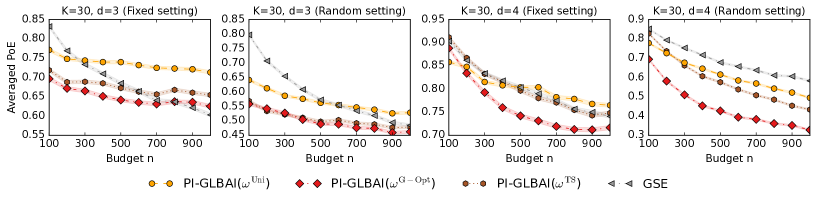
Figure 5: Average PoE with varying budgets for fixed and randomized settings in the GLB framework.

D.3 Choice of Baselines

A remark on TTTS.

Top two sampling algorithms is a family of algorithms that is known to have good performances in BAI. In Section 5, we used TS-TCI with $\beta=0.5$ from Jourdan et al. (2022) and denoted it as TTTS for sake of notation simplicity.

Choice of warm-up policy.

We evaluate different warm-up policies,TS and two Top-Two algorithms, TSTCI and T3C from Jourdan et al. (2022). The experiments shown in Figure 6 are run in the same setting as in Section 5, with $K=10$ arms in the MAB setting, and with $K=60$ and $d=4$ in the hierarchical setting. Figure 6 suggests to pick TS as a warm-up policy for the MAB setting and meTS for the hierarchical setting.

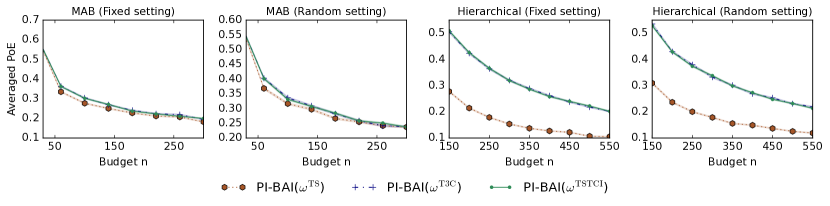
Figure 6: Average PoE of PI-BAI instantiated with different warm-up policies.

Influence of elimination.

We empirically compare the influence of using elimination on top of our methods. The elimination procedure is the same as the one used in Atsidakou et al. (2022). There are $\lfloor\log_{2}(K)\rfloor$ rounds, and each lasts $\lfloor\frac{n}{R}\rfloor$ steps. At each round, we pull each remaining arm $i$ $\lfloor\frac{\omega_{i}n}{R}\rfloor$ times. At the end of the round, half of arms are eliminated. These correspond to the arms that have the least posterior mean reward (so $\hat{\mu}_{n,i}$ in the MAB setting). The allocation $\omega$ is then normalized to allocate more budget to remaining arms. Note that we draft all observations at the end of each round, as it is the case in (Karnin et al., 2013; Azizi et al., 2021; Atsidakou et al., 2022). Figure 7 shows that using elimination does not give better performances, and hence we chose to not add these baselines in Section 5.

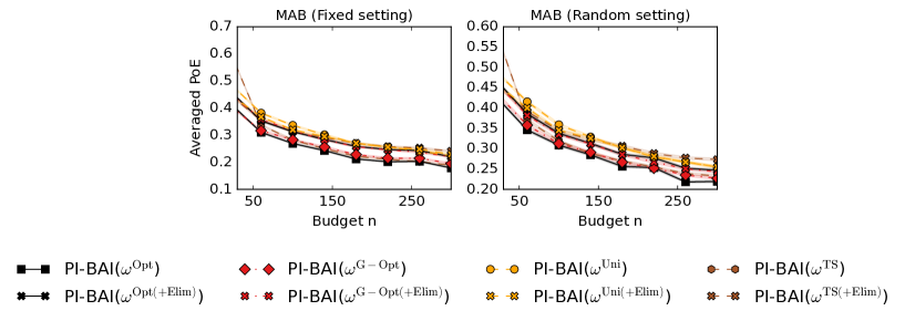
Figure 7: Average PoE of PI-BAI instantiated with different weights with or without elimination in the MAB setting.

D.4 Simple Regret

Figure 8 compares the performances of our methods based on the Bayesian simple regret $\mathbb{E}\left[\max_{i\in[K]}\theta-\theta_{J_{n}}\right]\,$, where the expectation is taken with respect to the prior distribution over instances $\theta$. Overall, it shows that our methods also have low simple regret in these settings.

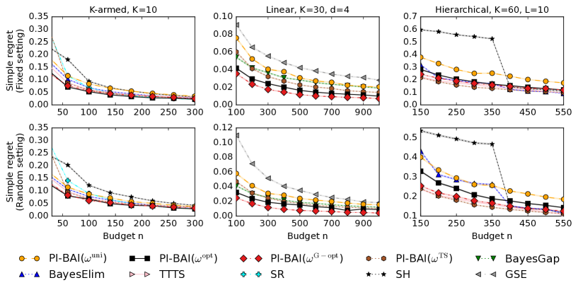
Figure 8: Average simple regret with varying budgets for fixed and randomized settings.

D.5 Confidence Intervals on Sampled Instances

We provide additional plots in the same settings of Section 5. The first row of Figure 9 shows the PoE of the methods averaged over 1000 different instances sampled from the prior distribution. For each instance, we repeat the experiments 100 times to get an estimate of the probability. We show one standard deviation around the averaged mean of PoE over instances. In the second row of the same figure, we plot the PoE of each method subtracted by the PoE of the method having the least PoE in each setting, that is, $\texttt{PI-BAI}(\omega^{\rm{opt}})$ in MAB, $\texttt{PI-BAI}(\omega^{\rm{G\shortminus opt}})$ in linear bandits and $\texttt{PI-BAI}(\omega^{\rm{TS}})$ in hierarchical bandits.

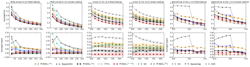
Figure 9: PoE of several methods (first row) and PoE of each method substracted by the PoE of the most performing method in each setting (second row). For each instance, we repeat the experiments 100 times and we average the results over 1000 instances. The confidence intervals show one standard deviation.

D.6 Benefits of Hierarchical Models

To illustrate the benefits of using a hierarchical structure (2.3), we compare the posterior variances $\hat{\sigma}^{2}_{n,i}$ under a standard model and a hierarchical model. The standard model is obtained by marginalizing over the effects $\mu$,

$$\theta_{i} \sim\mathcal{N}(b_{i}^{\top}\nu,\sigma^{2}_{0,i}+b_{i}^{\top}\Sigma b_{i}) \forall i\in[K]$$

$$Y_{t}\mid\mu,\theta,A_{t} \sim\mathcal{N}(\theta_{A_{t}},\sigma^{2}) \forall t\in[n]\,.$$ (33)

From (3), the corresponding posterior covariance of an arm $i\in[K]$ is

$$\hat{\sigma}^{-2}_{n,i}=\frac{1}{\sigma^{2}_{0,i}+b_{i}^{T}\Sigma b_{i}}+\frac{\omega_{i}n}{\sigma^{2}}\,.$$

For the first setting, we uniformly draw a vector $u\in[0,1]$ and set $\sigma_{0}=0.1u$ and $\Sigma=2I_{L}$. For the second setting, we set $\sigma_{0}=u$ and $\Sigma=10^{-3}I_{L}$. In both settings, we consider $K=50$ arms, and $L=10$ effects. We draw uniformly $\nu,b_{i}\in[-1,1]^{L}$ and the allocation vector is set to uniform allocation $\omega^{\rm{uni}}_{i}=\frac{1}{K}$ for any $i\in[K]$. In Figure 10 we plot the average posterior covariance $\frac{1}{K}\sum_{i\in[K]}\sigma^{2}_{n,i}$ across all arms for both the (marginalized) standard model (D.6) and the hierarchical model (2.3). The goal of this experiment is to show for which setting the benefits of the hierarchy are pronounced. The results show that this difference is more pronounced when the initial uncertainty of the effects $\Sigma$ is greater than the initial uncertainty of the mean rewards $(\sigma^{2}_{0,i})_{i\in[K]}$.

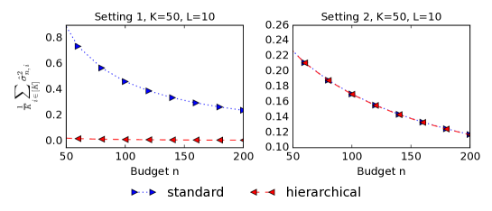
Figure 10: Average posterior covariance across all arms for standard and hierarchical model for two settings.

D.7 Hyperparameters

Warm-up length $n_{\rm{w}}$.

We try different values of warm-up length $n_{\rm{w}}$ for our warm-up policies. We emphasize that methods based on TTTS require $n_{\rm{w}}>K$ because each arm has to be pulled at the beginning. Figure 11 suggests picking $n_{\rm{w}}=2K$ for the warm)up with T3C and TSTCI, and $n_{\rm{w}}=K$ for the warm-up with TS.

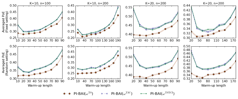
Figure 11: Average PoE of PI-BAI instantiated with different warm-up policies for different warm-up lengths $n_{\rm{w}}$.

Mixture parameter $\alpha$.

We discuss the choice of the mixture parameter $\alpha$. We recall that we use the heuristic $\alpha\omega^{\rm{opt}}_{i}+(1-\alpha)\frac{\mu_{0,i}\sigma_{0,i}}{\sum_{k\in[K]}\mu_{0,k}\sigma_{0,k}}$ in our experiments. Figure 12 shows that for the fixed setting, adding the vector $\frac{\mu_{0,i}\sigma_{0,i}}{\sum_{k\in[K]}\mu_{0,k}\sigma_{0,k}}$ helps improve the performances. This is not necessarily the case in the random setting.

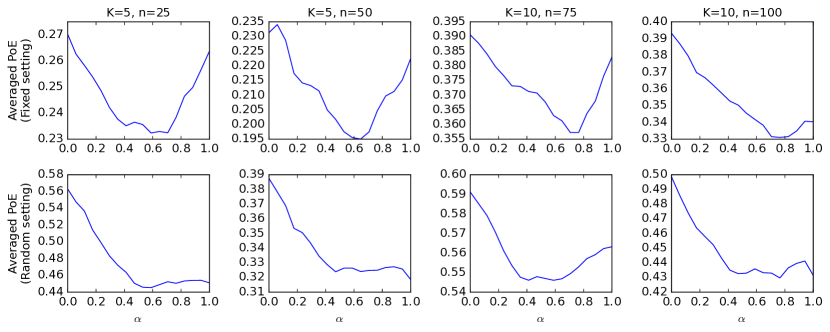
Figure 12: Average PoE of $\texttt{PI-BAI}(\omega^{\rm{opt}})$ for different mixture parameter $\alpha$.

D.8 Toy Experiments for $\omega^{\rm{opt}}$

We provide additional experiments to evaluate the optimized weights $\omega^{\rm{opt}}$ in different settings. In Figure 13, we set $K=3$, $\mu_{0}=(2,1.9,0)$, $(\sigma_{0,1},\sigma_{0,2},\sigma_{0,3})=(10^{-2},0.5,0.5)$. This corresponds to the motivating setting depicted in the introduction (Section 1). We provide a comprehensive illustration of the prior bandit instance $\mu_{0,i}\pm 2\sigma_{0,i}$ (left plot). Then we let the budget vary, $n\in[10,200]$, and for each $n$ we (numerically) optimize (11) to get $\omega^{\rm{opt}}_{n}$ (middle plot). On the right plot, we let the prior mean of arm 2 vary, $\mu_{0,2}\in[0,2]$, and get $\omega^{\rm{opt}}$ as a function of $\mu_{0,2}$. In Figure 14, we do the same experiments for 6 arms with 2 good arms a priori, $\mu_{0}=(2,1.9,1,0.6,0.3,0)$ and $\sigma_{0}$ uniformly spaced in $[0.5,0.1]$. As $n$ increases, $\omega^{\rm{opt}}$ suggests distributing roughly one third of the budget for each arm $1$ and $2$, and the remaining to the rest of the arms.

These results give insight on the behavior of $\omega^{\rm{opt}}$. In Figure 13, for small budgets, $\omega^{\rm{opt}}$ suggests pulling a lot the second arm because of its wide prior confidence $\sigma^{2}_{0,2}\gg\sigma^{2}_{0,1}$. It does not give much allocation to the last arm since it is statistically unlikely to become optimal. As the budget $n$ grows, most of the allocations are almost equal to arm 1 and arm 2. Since $\sigma^{2}_{0,1}\neq\sigma^{2}_{0,2}$, $\omega^{\rm{opt}}_{1}\neq\omega^{\rm{opt}}_{2}$ even for a large budget $n=200$. The right plot of Figure 13 shows that $\omega^{\rm{opt}}$ depends on prior gaps. Interestingly, this was not the case for the very special example $K=2$ depicted in Section 3.3.

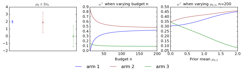
Figure 13: Illustration of the prior bandit instance (left), and optimized allocation $\omega^{\rm{opt}}$ when varying budget $n$ (middle) or one coordinate of $\mu_{0}$ (right).

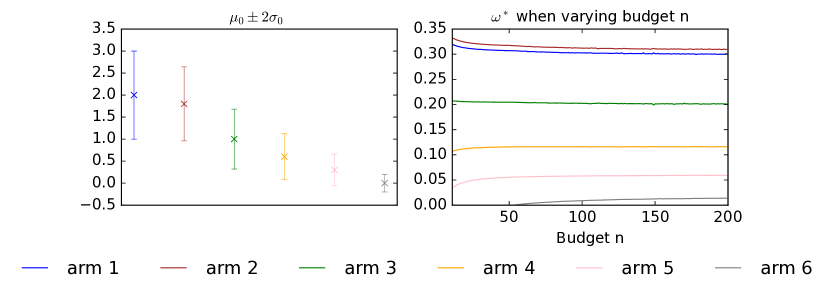
Figure 14: Illustration of the prior bandit instance (left), and optimized allocation $\omega^{\rm{opt}}$ when varying budget $n$ (right).

References

- Abbasi-Yadkori et al. (2011) Yasin Abbasi-Yadkori, David Pal, and Csaba Szepesvari. Improved algorithms for linear stochastic bandits. In Advances in Neural Information Processing Systems 24, pages 2312–2320, 2011.
- Alieva et al. (2021) Ayya Alieva, Ashok Cutkosky, and Abhimanyu Das. Robust pure exploration in linear bandits with limited budget. In International Conference on Machine Learning, pages 187–195. PMLR, 2021.
- Aouali (2023) Imad Aouali. Linear diffusion models meet contextual bandits with large action spaces. In NeurIPS 2023 Foundation Models for Decision Making Workshop, 2023.
- Aouali et al. (2023) Imad Aouali, Branislav Kveton, and Sumeet Katariya. Mixed-effect thompson sampling. In International Conference on Artificial Intelligence and Statistics, pages 2087–2115. PMLR, 2023.
- Atsidakou et al. (2022) Alexia Atsidakou, Sumeet Katariya, Sujay Sanghavi, and Branislav Kveton. Bayesian fixed-budget best-arm identification. arXiv preprint arXiv:2211.08572, 2022.
- Audibert et al. (2010) Jean-Yves Audibert, Sébastien Bubeck, and Rémi Munos. Best arm identification in multi-armed bandits. In COLT, pages 41–53, 2010.
- Azizi et al. (2023) Javad Azizi, Branislav Kveton, Mohammad Ghavamzadeh, and Sumeet Katariya. Meta-learning for simple regret minimization. In Proceedings of the AAAI Conference on Artificial Intelligence, volume 37, pages 6709–6717, 2023.
- Azizi et al. (2021) Mohammad Javad Azizi, Branislav Kveton, and Mohammad Ghavamzadeh. Fixed-budget best-arm identification in structured bandits. arXiv preprint arXiv:2106.04763, 2021.
- Basu et al. (2021) Soumya Basu, Branislav Kveton, Manzil Zaheer, and Csaba Szepesvari. No regrets for learning the prior in bandits. In Advances in Neural Information Processing Systems 34, 2021.
- Bishop (2006) Christopher M Bishop. Pattern Recognition and Machine Learning, volume 4 of Information science and statistics. Springer, 2006.
- Bubeck et al. (2009) Sébastien Bubeck, Rémi Munos, and Gilles Stoltz. Pure exploration in multi-armed bandits problems. In Algorithmic Learning Theory: 20th International Conference, ALT 2009, Porto, Portugal, October 3-5, 2009. Proceedings 20, pages 23–37. Springer, 2009.
- Carpentier and Locatelli (2016) Alexandra Carpentier and Andrea Locatelli. Tight (lower) bounds for the fixed budget best arm identification bandit problem. In Conference on Learning Theory, pages 590–604. PMLR, 2016.
- Chapelle and Li (2012) Olivier Chapelle and Lihong Li. An empirical evaluation of Thompson sampling. In Advances in Neural Information Processing Systems 24, pages 2249–2257, 2012.
- Degenne (2023) Rémy Degenne. On the existence of a complexity in fixed budget bandit identification. arXiv preprint arXiv:2303.09468, 2023.
- Even-Dar et al. (2006) Eyal Even-Dar, Shie Mannor, Yishay Mansour, and Sridhar Mahadevan. Action elimination and stopping conditions for the multi-armed bandit and reinforcement learning problems. Journal of machine learning research, 7(6), 2006.
- Filippi et al. (2010) Sarah Filippi, Olivier Cappe, Aurelien Garivier, and Csaba Szepesvari. Parametric bandits: The generalized linear case. In Advances in Neural Information Processing Systems 23, pages 586–594, 2010.
- Hoffman et al. (2014) Matthew Hoffman, Bobak Shahriari, and Nando Freitas. On correlation and budget constraints in model-based bandit optimization with application to automatic machine learning. In Artificial Intelligence and Statistics, pages 365–374. PMLR, 2014.
- Hong et al. (2020) Joey Hong, Branislav Kveton, Manzil Zaheer, Yinlam Chow, Amr Ahmed, and Craig Boutilier. Latent bandits revisited. In Advances in Neural Information Processing Systems 33, 2020.
- Hong et al. (2022a) Joey Hong, Branislav Kveton, Sumeet Katariya, Manzil Zaheer, and Mohammad Ghavamzadeh. Deep hierarchy in bandits. arXiv preprint arXiv:2202.01454, 2022a.
- Hong et al. (2022b) Joey Hong, Branislav Kveton, Manzil Zaheer, and Mohammad Ghavamzadeh. Hierarchical Bayesian bandits. In Proceedings of the 25th International Conference on Artificial Intelligence and Statistics, 2022b.
- Hong et al. (2023) Joey Hong, Branislav Kveton, Manzil Zaheer, Sumeet Katariya, and Mohammad Ghavamzadeh. Multi-task off-policy learning from bandit feedback. In International Conference on Machine Learning, pages 13157–13173. PMLR, 2023.
- Jourdan et al. (2022) Marc Jourdan, Rémy Degenne, Dorian Baudry, Rianne de Heide, and Emilie Kaufmann. Top two algorithms revisited. Advances in Neural Information Processing Systems, 35:26791–26803, 2022.
- Karnin et al. (2013) Zohar Karnin, Tomer Koren, and Oren Somekh. Almost optimal exploration in multi-armed bandits. In International conference on machine learning, pages 1238–1246. PMLR, 2013.
- Katz-Samuels et al. (2020) Julian Katz-Samuels, Lalit Jain, Kevin G Jamieson, et al. An empirical process approach to the union bound: Practical algorithms for combinatorial and linear bandits. Advances in Neural Information Processing Systems, 33:10371–10382, 2020.
- Kaufmann et al. (2016) Emilie Kaufmann, Olivier Cappé, and Aurélien Garivier. On the complexity of best arm identification in multi-armed bandit models. Journal of Machine Learning Research, 17:1–42, 2016.
- Komiyama et al. (2023) Junpei Komiyama, Kaito Ariu, Masahiro Kato, and Chao Qin. Rate-optimal bayesian simple regret in best arm identification. Mathematics of Operations Research, 2023.
- Kveton et al. (2020) Branislav Kveton, Manzil Zaheer, Csaba Szepesvari, Lihong Li, Mohammad Ghavamzadeh, and Craig Boutilier. Randomized exploration in generalized linear bandits. In International Conference on Artificial Intelligence and Statistics, pages 2066–2076. PMLR, 2020.
- Kveton et al. (2021) Branislav Kveton, Mikhail Konobeev, Manzil Zaheer, Chih-Wei Hsu, Martin Mladenov, Craig Boutilier, and Csaba Szepesvari. Meta-Thompson sampling. In Proceedings of the 38th International Conference on Machine Learning, 2021.
- Lam and Herlocker (2016) Shyong Lam and Jon Herlocker. MovieLens Dataset. http://grouplens.org/datasets/movielens/, 2016.
- Lattimore and Szepesvári (2020) Tor Lattimore and Csaba Szepesvári. Bandit algorithms. Cambridge University Press, 2020.
- Lee et al. (2023) Jongyeong Lee, Junya Honda, and Masashi Sugiyama. Thompson exploration with best challenger rule in best arm identification. arXiv preprint arXiv:2310.00539, 2023.
- Li et al. (2017) Lisha Li, Kevin Jamieson, Giulia DeSalvo, Afshin Rostamizadeh, and Ameet Talwalkar. Hyperband: A novel bandit-based approach to hyperparameter optimization. The journal of machine learning research, 18(1):6765–6816, 2017.
- López-Fidalgo (2023) Jesús López-Fidalgo. Optimal Experimental Design: A Concise Introduction for Researchers, volume 226. Springer Nature, 2023.
- Nguyen and Vernade (2023) Nicolas Nguyen and Claire Vernade. Lifelong best-arm identification with misspecified priors. In Sixteenth European Workshop on Reinforcement Learning, 2023.
- Peleg et al. (2022) Amit Peleg, Naama Pearl, and Ron Meir. Metalearning linear bandits by prior update. In International Conference on Artificial Intelligence and Statistics, pages 2885–2926. PMLR, 2022.
- Phan et al. (2019) My Phan, Yasin Abbasi Yadkori, and Justin Domke. Thompson sampling and approximate inference. Advances in Neural Information Processing Systems, 32, 2019.
- Qin (2022) Chao Qin. Open problem: Optimal best arm identification with fixed-budget. In Conference on Learning Theory, pages 5650–5654. PMLR, 2022.
- Russo (2016) Daniel Russo. Simple bayesian algorithms for best arm identification. In Conference on Learning Theory, pages 1417–1418. PMLR, 2016.
- Simchowitz et al. (2021) Max Simchowitz, Christopher Tosh, Akshay Krishnamurthy, Daniel Hsu, Thodoris Lykouris, Miro Dudik, and Robert Schapire. Bayesian decision-making under misspecified priors with applications to meta-learning. In Advances in Neural Information Processing Systems 34, 2021.
- Urteaga and Wiggins (2018) Inigo Urteaga and Chris Wiggins. Variational inference for the multi-armed contextual bandit. In Proceedings of the 21st International Conference on Artificial Intelligence and Statistics, pages 698–706, 2018.
- Virtanen et al. (2020) Pauli Virtanen, Ralf Gommers, Travis E. Oliphant, Matt Haberland, Tyler Reddy, David Cournapeau, Evgeni Burovski, Pearu Peterson, Warren Weckesser, Jonathan Bright, Stéfan J. van der Walt, Matthew Brett, Joshua Wilson, K. Jarrod Millman, Nikolay Mayorov, Andrew R. J. Nelson, Eric Jones, Robert Kern, Eric Larson, C J Carey, İlhan Polat, Yu Feng, Eric W. Moore, Jake VanderPlas, Denis Laxalde, Josef Perktold, Robert Cimrman, Ian Henriksen, E. A. Quintero, Charles R. Harris, Anne M. Archibald, Antônio H. Ribeiro, Fabian Pedregosa, Paul van Mulbregt, and SciPy 1.0 Contributors. SciPy 1.0: Fundamental Algorithms for Scientific Computing in Python. Nature Methods, 17:261–272, 2020. doi: 10.1038/s41592-019-0686-2.
- Wainwright et al. (2008) Martin J Wainwright, Michael I Jordan, et al. Graphical models, exponential families, and variational inference. Foundations and Trends® in Machine Learning, 1(1–2):1–305, 2008.
- Wang et al. (2023) Po-An Wang, Kaito Ariu, and Alexandre Proutiere. On uniformly optimal algorithms for best arm identification in two-armed bandits with fixed budget. arXiv preprint arXiv:2308.12000, 2023.
- Wolke and Schwetlick (1988) R. Wolke and H. Schwetlick. Iteratively reweighted least squares: Algorithms, convergence analysis, and numerical comparisons. SIAM Journal on Scientific and Statistical Computing, 9(5):907–921, 1988.
- Yang and Tan (2022) Junwen Yang and Vincent Tan. Minimax optimal fixed-budget best arm identification in linear bandits. Advances in Neural Information Processing Systems, 35:12253–12266, 2022.