Quantum Anomalous Hall Effect in $d$-Electron Kagome Systems: Chern Insulating States from Transverse Spin-Orbit Coupling

Abstract

Inspired by the discovery of metal-organic frameworks, the possibility of quantum anomalous Hall effect (QAHE) in two-dimensional kagome systems with $d$-orbital electrons is studied within a multi-orbital tight-binding model. In the absence of exchange-type spin-orbit coupling, isotropic Slater-Koster integrals give a band structure with relativistic (Dirac) and quadratic band crossing points at high symmetry spots in the Brillouin zone. A quantized topological invariant requires a flux-creating spin-orbit coupling, giving Chern number (per spin sector) $C=1$ not only from the familiar Dirac points at the six corners of the Brillouin zone, but also from the quadratic band crossing point at the center $\Gamma$. Surprisingly, this QAHE comes from the nontrivial effective flux induced by the transverse part of the spin-orbit coupling, exhibited by electrons in the $d$-orbital state with $m_{l}=0$ ($d_{z^{2}}$ orbital), in stark contrast to the more familiar form of QAHE due to the $d$-orbitals with $m_{l}\neq 0$, driven by the Ising part of spin-orbit coupling. The $C=1$ Chern plateau (per spin sector) due to Dirac point extends over a smaller region of Fermi energy than that due to quadratic band crossing. Our result hints at the promising potential of kagome metal-organic frameworks as a platform for dissipationless electronics by virtue of its unique QAHE.

Introduction.—Anomalous Hall effect (AHE) refers to a transport phenomenon where an electric current produces a voltage perpendicular to the former, in the absence of external magnetic field but with broken time-reversal symmetry. Usually occurring in ferromagnetic materials  AHErmp , its foundation was built in pioneering works  KarplusLuttinger ; Smit ; Luttinger ; Kondo ; Berger ; Nozieres . More recent progress investigates this effect in magnetic semiconductors  JungwirthPRL and metallic ferromagnets OnodaNagaosaJPSJ ; KontaniPRB2007 .

Theoretical studies of two-dimensional materials underline the significance of electronic structures with Dirac points and flatbands Flatband1 ; Flatband2 ; Flatband3 , which have been reported in inorganic-metal compounds DiracFlatbandKagome . Lately, a class of materials; kagome metal-organic frameworks, has been synthesized  Zhang ; Hua ; Shaiek and studied using ab-initio first-principle calculations Denawi . These materials offer an alternative venue for such fascinating phenomena as high-temperature fractional quantum Hall effect  Flatband3 , frustration-induced quantum spin liquid state MakhfudzPRB2014  SavaryBalentsRPP , magnetization plateaus from spin gap  NatCommsHotta  CapponiPRB2013  MakhfudzPujolPRL2015 , and prospectively the AHE.

The AHE may arise from intrinsic mechanisms associated with non-collinear or chiral spin order  Taguchi ; YePRL ; OnodaNagaosaPRL2 ; MartinBatista ; OhgushiPRB ; ZFangScience ; CanalsPRB ; MacDonaldPRL ; BrunoPRL ; MacDonaldPRL ; MakhfudzPujolPRB2015 or from the Berry curvature in reciprocal $\mathbf{k}$ space  SundaramNiu ; Sinitsyn , representing the topological property of the band structure of the electrons  Haldane2004PRL characterized by Chern number TKNN , an integer AHErmp . The latter mechanism gives rise to the quantum anomalous Hall effect (QAHE)  MacDonaldRMP as shown theoretically in honeycomb  Haldane1988PRL  OnodaNagaosaPRL1 and kagome KSunPRL2009 lattices, magnetized graphene QAHEgrapheneAFM  QAHEinGraphene , semiconductor quantum wells  CXLiuPRL ; CXLiuAnnCondMat and observed experimentally in magnetic topological insulators Science  ScienceDeng , so far relying on the gap at the Dirac or semi-Dirac point Vanderbilt . The QAHE is also present in kagome systems either in organic QAHE2DorganicTI ; PRLabinitiMOF ; SciRep or inorganic frameworks SCZhangPRL  Nature2018 , highlighting the importance of the effect in $d$-orbital systems (where the conduction electrons have angular momentum quantum numbers $l=2$ and $m_{l}=0,\pm 1,\pm 2$) SCZhangPRL ; Nature2018 ; QAHE2DorganicTI , but an analytical multi-orbital theory that probes the insulating Chern states at all nontrivial gaps induced by spin-orbit coupling (SOC) beyond the Ising approximation is still lacking.

This manuscript addresses the possible occurrence of quantum anomalous Hall effect in the $d$-orbital kagome metal-organic frameworks (MOFs), focusing on the Berry curvature intrinsic mechanism, based on an analytical tight-binding model. Going beyond the Ising limit of spin-polarized bands, we show that a quantum anomalous Hall state with $C=1$ per spin sector can arise from the Berry curvature of the bands of the $m_{l}=0$ $d$-orbital ($d_{z^{2}}$ orbital) at their quadratic band crossing (QBC) point and, crucially, relies on the transverse part of the spin-orbit interaction that generates an orbital-dependent effective flux. This QAHE due to the QBC point accompanies the more familiar QAHE due to the Dirac point.

Model — The conduction electrons of the kagome MOFs are descibed by a tight-binding Hamiltonian with nearest-neighbour hopping and spin-orbit coupling :

$$H=\sum_{\begin{subarray}{c}\langle ij\rangle\\ \alpha\alpha^{\prime}\sigma\end{subarray}}t_{ij,\alpha\alpha^{\prime}}d^{{\dagger}}_{i,\alpha\sigma}d_{j,\alpha^{\prime}\sigma}+\mathrm{h.c.}+\sum_{\begin{subarray}{c}i\\ \alpha\sigma\end{subarray}}E_{\alpha}d^{{\dagger}}_{i,\alpha\sigma}d_{i,\alpha\sigma}\\ -\sum_{\begin{subarray}{c}i\\ \alpha\sigma\sigma^{\prime}\end{subarray}}d^{{\dagger}}_{i,\alpha\sigma}\left(\mathbf{M}\cdot\mathbf{s}\right)_{\sigma,\sigma^{\prime}}d_{i,\alpha\sigma^{\prime}}\\ +\lambda_{OS}\sum_{\begin{subarray}{c}i\\ \alpha\sigma\alpha^{\prime}\sigma^{\prime}\end{subarray}}d^{{\dagger}}_{i,\alpha\sigma}\left(\mathbf{l}\cdot\mathbf{s}\right)_{\alpha\sigma,\alpha^{\prime}\sigma^{\prime}}d_{i,\alpha^{\prime}\sigma^{\prime}}\\ +i\lambda\sum_{\begin{subarray}{c}\langle ij\rangle\\ \alpha\sigma,\alpha^{\prime}\sigma^{\prime}\end{subarray}}\nu_{ij}d^{{\dagger}}_{i,\alpha\sigma}\left(\mathbf{l}\cdot\mathbf{s}\right)_{\alpha\sigma,\alpha^{\prime}\sigma^{\prime}}d_{j,\alpha^{\prime}\sigma^{\prime}}+\mathrm{h.c}\,\text{.}$$ (1)

$d^{{\dagger}}_{i,\alpha\sigma}(d_{i,\alpha\sigma})$ are creation (annihilation) operators for $d$-electrons of spin $\sigma$ in orbital $\alpha$ and on site $i$ (Fig.1), and the hopping matrix elements $t_{ij,\alpha\alpha^{\prime}}$ in the first term are given by $t_{ij;\alpha,\alpha^{\prime}}=f_{\sigma}V_{dd\sigma}+f_{\pi}V_{dd\pi}+f_{\delta}V_{dd\delta}$, where $f_{\sigma/\pi/\delta}$ are $\alpha,\alpha^{\prime}$-dependent simple algebraic functions of nearest-neighbor vectors indices and the $V_{dd(\sigma/\pi/\delta)}$ are the Slater-Koster integrals for hopping of electrons between two $d$ orbitals that can be of $\sigma,\pi$, or $\delta$ type, available from the Slater-Koster table Harrison  SupplementaryMaterials . The second term accounts for the onsite energies which can adopt three different values: $E_{1}$ for the $d_{z^{2}}$-orbital, $E_{2}$ for the $d_{xz}$ and $d_{yz}$-orbital, and $E_{3}$ for $d_{xy}$ and $d_{x^{2}-y^{2}}$. The third term represents the spin splitting due to a ferromagnetic exchange field $\mathbf{M}$ arising from the spin of the transition metal ion, which we assume to be perpendicular to the lattice. The last two contributions (onsite and transfer (exchange-type) SOCs) account for the intrinsic SOCs on a given site and between nearest neighbours. The latter term has to be preceded by an imaginary $i$ since the matrix elements $\nu_{ij}=\pm 1$ change sign according to whether the hopping occurs clockwise or counterclockwise around a triangle. Note that the inclusion of the operator $\mathbf{l}$ allows us to extend the Kane-Mele SOC KaneMelePRL to multi-orbital systems and going past the Ising approximation of spin-polarized bands.

Band Structure.—The physics of the conduction electrons can be deduced from the band structure computed from diagonalizing the Hamiltonian Eq.(1) in the basis of the electron state (5 orbitals times 3 sublattices times 2 spin states). Presented in Fig.2 is the band structure for the spin up state; the lower energy state of interest, lower by typically few ($\sim 1.0$ to $3.0$) eV than the spin down state due to the exchange field $M_{z}$Denawi .

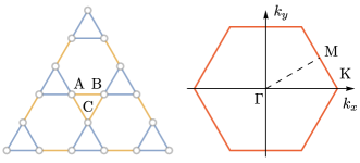
Figure 1: The kagome lattice (left) with its three sublattices and its first Brillouin zone (right) with the high-symmetry points.

Ab-initio calculations for the TM₃C₆O₆ family of metal organic compounds give a particularly simple $s$-orbital electron-like band structure in the energy range near zero energy (charge neutrality) especially in the beginning of 3$d$ series Denawi . Setting the tight-binding parameters to mimic the ab-initio band structure, the $s$-electron-like profile can be reproduced by assigning equal value $V_{dd\sigma}=V_{dd\delta}=V_{dd\pi}$ for the Slater-Koster integrals in our tight-binding model, resulting in a flat band and two dispersive bands touching each other at the Dirac point at K and the QBC at $\Gamma$ as shown in the inset of Fig. 2a), as also found in existing works DiracFlatbandKagome . The on-site energies $E_{\alpha}$ separate the different $d$-orbitals from each other in the realistic band structure, but eventually, these on-site energies do not influence the main result in an essential way SupplementaryMaterials .

Adding transfer SOC opens up a gap, as illustrated in Fig. 2a). The Ising part $l_{z}s_{z}$ of this SOC opens up a gap of order $\mathcal{O}(\lambda)$ at the gapless points, not just the Dirac point at K, but also the quadratic band crossing point at $\Gamma$, except for the $d_{z^{2}}$ orbital because of its $m_{l}=0$. For this “trivial” $d$-orbital, the planar part $l_{x}s_{x}+l_{y}s_{y}$ of the transfer SOC opens up a small gap at the quadratic band crossing at $\Gamma$ while opening a much smaller gap at the Dirac point at K SupplementaryMaterials . To probe the presence of a gap we compute the density of states using the tight-binding model parameters that mimic the ab-initio band structure  Denawi . The result is shown in Fig. 2b), where the gaps at the QBC and Dirac points give zero density of states.

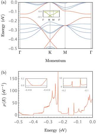
Figure 2: a) Band structure of $d$-orbital electrons in the low energy spin-up sector along the $K-\Gamma-M-\Gamma$ path in the first Brillouin zone (Fig.1) for the kagome model Eq.(1) with  Note $E_{1}=E_{2}=E_{3}=0.25$eV, $V_{dd\pi}=V_{dd\delta}=V_{dd\sigma}=-0.25$eV, $\lambda=0.19$eV and $\lambda_{OS}=0.0$eV, and $M_{z}=1.0,M_{x}=M_{y}=0.0$ all in eV. The three bands of $d_{z^{2}}$ orbital are highlighted by red curves. The small inset shows the band structure without SOCs; i.e. $\lambda=\lambda_{OS}=0.0$eV, for which all the five $d$-orbitals become degenerate. b) The corresponding tight-binding total density of states $\rho(E)$ from all five $d$-orbitals in the spin up sector. The visible intervals with vanishing density of states correspond to the gaps acquired by the ${d}_{z^{2}}$ orbital, at the Dirac and QBC points as marked by insets on the top left and right corners, respectively.

Berry Curvature and Chern Number.—In the intrinsic mechanism for the anomalous Hall effect, the transverse motion of the electron is caused by the “anomalous velocity”, proportional to the cross product of the electric field and the Berry curvature $\Omega(\mathbf{k})$ defined in momentum space  Haldane2004PRL . This Berry curvature acts as an effective magnetic field in momentum space. Integrating this field over a surface in 2D $\mathbf{k}$ space gives rise to a topological magnetic charge, which is essentially the Chern number characterizing the anomalous quantum Hall effect  TKNN . At arbitrary temperature $T$, the Berry curvature field is given by  AHErmp

$$\Omega(\mathbf{k})=\hbar^{2}\sum_{n\neq n^{\prime}}G_{nn^{\prime}}(\mathbf{k})\mathrm{Im}\left[\frac{\langle\psi_{n\mathbf{k}}|v_{x}(\mathbf{k})|\psi_{n^{\prime}\mathbf{k}}\rangle\langle\psi_{n^{\prime}\mathbf{k}}|v_{y}(\mathbf{k})|\psi_{n\mathbf{k}}\rangle}{\left(\varepsilon_{n^{\prime}\mathbf{k}}-\varepsilon_{n\mathbf{k}}\right)^{2}}\right]$$ (2)

with

$$G_{nn^{\prime}}(\mathbf{k})=f(\epsilon_{n}(\mathbf{k}))-f(\epsilon_{n^{\prime}}(\mathbf{k}))$$ (3)

where $f(\epsilon_{n}(\mathbf{k}))=(\exp(\beta(\epsilon_{n}(\mathbf{k})-E_{F}))+1)^{-1}$ for which $\beta=1/(k_{B}T)$ with Boltzmann constant $k_{B}$ and reduced Planck constant $\hbar$, $\mathrm{Im}$ indicates the imaginary part of its argument, $\psi_{n\mathbf{k}},\varepsilon_{n\mathbf{k}}$ are respectively the eigenfunction and eigenvalue of the $n^{\mathrm{th}}$-eigenstate of $H_{\mathbf{k}}$ while the velocity operator is given by $v_{x}=(1/\hbar)\partial H_{\mathbf{k}}/\partial k_{x}$ and similarly for the $y$ part. The profile of the Berry curvature field is illustrated in Fig.3.

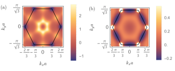
Figure 3: Color maps of the (dimensionless) Berry curvature field $a^{-2}\Omega(k_{x}a,k_{y}a)$ where $a$ is the lattice spacing, taken as the reference unit of length, with the same parameters as those for Fig. 2b) evaluated at a) $E_{F}=-0.150$eV for the QBC and b)$E_{F}=-0.414$eV for the Dirac point, within the gaps of the band structure with SOC as shown in Fig. 2. The peaks of $a^{-2}\Omega(k_{x}a,k_{y}a)$ are located a) around the center of BZ ($\Gamma$ point) and b) at the corners of BZ and are responsible for the Chern plateaus in Fig.4.

The corresponding Chern number is then evaluated over the Brillouin zone

$$C=\frac{1}{2\pi}\int_{\mathrm{BZ}}d^{2}\mathbf{k}\Omega(\mathbf{k})=\frac{\Phi}{2\pi}$$ (4)

linked to the Berry phase $\Phi$  Haldane2004PRL , giving an intrinsic Hall conductivity $\sigma_{xy}=(e^{2}/h)C$ where $e$ is the elementary charge of electron and $h$ is the Planck constant. As shown in  AHErmp , the Chern number can also be recast in terms of intraband processes and computed efficiently using a trick based on a unitary transformation function  Fukui . In the present work, the interband definition of Chern number is used.

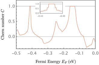
Figure 4: The dependence of the Chern number $C$ on the Fermi energy $E_{F}$ (eV) at $T=0.0001$eV($=1.1$Kelvin) for kagome metal-organic framework with the same parameters as those for Fig. 2b). Clear plateaus at $C=1$ fall within the gaps of the $d_{z^{2}}$ orbital, centered at about -0.150eV for gapped QBC point at $\Gamma$ and -0.414eV for gapped Dirac point at K in Fig.2.

QAHE from Gapped Quadratic Band Crossing.—The Chern number is computed from the full $30\times 30$ Hamiltonian matrix using Eq.(2), focusing on the spin up sector just below the zero Fermi energy, at $T=0.0001$eV ($=1.1$Kelvin), low enough to enter the quantum regime while still being within reach of existing cryogenic technology.

The resulting profile of the Chern number is shown in Fig. 4 as function of the Fermi energy. The computed topological invariant (proportional to the anomalous Hall conductivity) is mostly nonzero and varies continuously with Fermi energy, but may display exact quantization (integer Chern number) within the spin-orbit coupling-induced gap, appearing as plateau. These plateaus are clearly visible in Fig. 4, showing Chern number at quantized value $C=1$, corresponding to a quantized Hall conductivity $\sigma_{xy}=e^{2}/h$. It can be verified by comparing with Fig. 2a) that the plateaus fall within the gaps of the band structure of the $d_{z^{2}}$ orbital in the spin up sector.

Interestingly, one of the $C=1$ Chern plateaus comes from the QBC point at the center $\Gamma$ of the Brillouin zone, as reflected by the peak of the Berry curvature field at the center in Fig. 4a), and thus corresponds to non-relativistic electrons associated with the normally considered irrelevant $d_{z^{2}}$ orbital. This $C=1$ Chern plateau corresponds to a Berry phase $\Phi=2\pi$ originating from a QBC point in a system with $C_{6}$ symmetry KSunPRL2009 . The associated QAHE is robust, giving a Chern plateau whose width is proportional to $\lambda$. Noting that the Chern plateau occurs just (slightly) below the zero Fermi energy, this implies that the QAHE requires hole doping concentration corresponding to 1/3 filling factor into the system, because one has to deplete the flatband of electrons while leaving the lower two bands occupied (see the inset of Fig. 2a)).

The gapped Dirac points corresponding to the $d_{z^{2}}$ orbital, located at the six corners ($\pm$K) of the Brillouin zone, also display a $C=1$ Chern plateau. Due to the smaller gap at the Dirac point, the plateau lies in a tiny region of Fermi energy with much smaller width (by an order of magnitude or more) than that at the QBC. More precisely, for reasonable sets of parameters with $\lambda$ a few hundreds meV as used to produce the figures in this main text, the gap at the Dirac point is less than 10 meV, whereas that at the QBC is several tens of meV, as illustrated in Fig. 4 SupplementaryMaterials . In real materials, SOC is usually weak but the Chern plateau at the QBC gap is still expected to be broader than the one at the Dirac gap, thus rendering the QAHE from the QBC point more prominent. Furthermore, since the energy of the Dirac point is further below the Fermi energy (see Fig. 2a), corresponding to $1/3$ filling factor of the spin up band, the QAHE from such Dirac point would require an amount of hole doping equivalent to 2/3 filling factor (because one has to vacate both the flat band and middle band of electrons while leaving the lowest band occupied (inset of Fig. 2a)), larger than that for QAHE due to QBC. Hence, in materials with weak SOC, the QBC Chern insulating state will be more dominant than that due to the Dirac point.

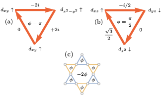
Figure 5: Representative effective fluxes induced by the a) Ising part and b) transverse part of exchange SOC, with the orbital state at the site and the resulting (generally complex) number indicating the overlap $\langle\alpha,s|l_{a}s_{a}|\alpha^{\prime},s^{\prime}\rangle$ where $\alpha,s$ are the orbital, spin indices (marked by spin up or down arrow) while $a=x,y,z$ and c) the resulting flux pattern. Only when the hopping is induced by the transverse part of the exchange SOC $l_{x}s_{x}+l_{y}s_{y}$ involving spin flip and a $d_{z^{2}}$ orbital state, will $\phi$ be nontrivial $\phi\neq 0,\pi$ and thus breaks time-reversal symmetry, as exemplified in b). All other contributions give trivial (non-time-reversal symmetry-breaking) fluxes SupplementaryMaterials .

On the other hand, the $d_{xy}$ and $d_{x^{2}-y^{2}}$ orbitals are found to give trivial Chern ($C=0$) plateau within the gap at any spin-orbit coupling strength $\lambda$; this clearly relates to a non-perturbative topological origin and in fact pertains to the effective flux  SupplementaryMaterials . More precisely, adopting the flux analysis method KontaniJPSJ762007main  KontaniPRL2008main , for the kagome lattice the electron hopping induces fluxes $\phi$ through the triangles and $-2\phi$ through the hexagons, giving zero average flux per unit cell  OhgushiPRB . The value of $\phi$ depends on the combination of the orbitals  SupplementaryMaterials resulting in time-reversal symmetry breaking, unless $\phi$ is 0 or $\pi$ (referred here as “trivial”). The fluxes turn out to be trivial for exchange-type SOC-induced hoppings involving only the “nontrivial” $d$-orbitals ($d_{xz},d_{yz},d_{xy},d_{x^{2}-y^{2}}$) whereas the fluxes are nontrivial for spin-flipping hoppings between the $d_{z^{2}}$ orbital and the other four orbitals, made possible by the transverse part of the SOC $l_{x}s_{x}+l_{y}s_{y}$, as illustrated in Fig.5. This explains why the $d_{z^{2}}$ orbital gives rise to the QAHE with its Chern plateaus. The remaining two orbitals $d_{xz}$ and $d_{yz}$, both of which are odd under $z\rightarrow-z$ mirror reflection, do not give rise to a Chern insulating state at all  SupplementaryMaterials . Due to the topological flux origin of the Chern insulating state where the flux is independent of the strength of SOC, the state exists at arbitrarily small but nonzero $\lambda>0$, with $C=1$ Chern plateaus at the QBC and Dirac points of the $d_{z^{2}}$ orbital.

For three candidate materials in the TM₃C₆O₆ family with TM = Sc, Ti, V, ab-initio band structure calculation  Denawi indicates that all of them have some finite densities of states for the $d_{z^{2}}$ orbital at or just below the zero Fermi energy, with Sc₃C₆O₆ having the most dominant content of $d_{z^{2}}$. This suggests that the predicted QAHE based on $d_{z^{2}}$ orbital is expected to be applicable to these real kagome organic metal compounds.

Discussion and Conclusions.—We have demonstrated a mechanism for the emergence of the quantum anomalous Hall effect (QAHE) in kagome $d$-systems due to the transverse part of the exchange-type intrinsic spin-orbit coupling (SOC) which is applicable to kagome metal organic frameworks. The phenomenon involves $d$-orbital electrons with $m_{l}=0$ ($d_{z^{2}}$ orbital) and the main contribution arises from the non-relativistic spectrum at the quadratic band crossing (QBC) point at the center of the Brillouin zone, instead of the usual relativistic Dirac spectrum at the corners of the Brillouin zone  SCZhangPRL  Nature2018 or semi-Dirac spectrum  Vanderbilt . The spectrum is gapped by the transverse part, rather than Ising part of the exchange-type SOC. All the other four $d$-orbitals give no QAHE, a scenario quite distinct and unexpected compared to existing works where normally these more “nontrivial” $d$-orbitals are considered to be responsible for the anomalous Hall effect  KontaniPRB2007  SCZhangPRL .The QAHE in the presence of exchange-type SOC has contributions both due to the QBC and Dirac points of the $d_{z^{2}}$ orbital, but the bandwidth of Chern plateau in the former is significantly broader than the latter, in principle making the QAHE due to the QBC easier to achieve and detect as compared to the QAHE associated to the Dirac point. The demonstrated QAHE requires lower amount of doping in the case of the QBC point, thus offering an alternative route toward the realization of dissipationless electronic devices.

Acknowledgements.—I.M. thanks Dr. Y. Hajati and M. Alipourzadeh for useful discussion on spin-orbit coupling and past collaboration on related topic.

Supplementary Materials: Quantum Anomalous Hall Effect in $d$-Electron Kagome Systems: Chern Insulating States from Transverse Spin-Orbit Coupling
I. Makhfudz¹, M. Cherkasskii², P. Lombardo¹, S. Schäfer¹, S. V. Kusminskiy ^2,3, and R. Hayn¹

¹IM2NP, UMR CNRS 7334, Aix-Marseille Université, 13013 Marseille, France
²Institut für Theoretische Festkörperphysik, RWTH Aachen University, 52056 Aachen, Germany
³Max Planck Institute for the Science of Light, Staudtstraße 2, PLZ 91058 Erlangen, German

In these Supplementary Materials, we provide additional details supplementing the main text. First, the basis states with respect to which the Hamiltonian matrix is written, the Slater-Koster integrals, and the diagonalization of the resulting matrix are described. Then, we provide the plots of the band structure and its evolution when varying the parameter of utmost interest; the exchange-type (transfer) spin-orbit coupling. Next, we give the computed Chern number as function of Fermi energy from the non-trivial $d$-orbitals. Afterwards, the physical origin of the quantum anomalous Hall effect from the effective flux induced by the transfer spin-orbit coupling is explained in detail, including why the nontrivial Chern plateaus come from the trivial $d$-orbital. Finally, the role of (or absence thereof) onsite spin-orbit coupling in quantum anomalous Hall effect is discussed.

I Basis States and Diagonalization of Hamiltonian Matrix

We focus on d-band electrons, which have angular momentum $l=2$ and spin $s=1/2$. The Hamiltonian matrix corresponding to Eq.(1) in the main text is written in the basis states involving the five $d$-orbitals, three sublattices, and two spin states (up and down spin).

The five $d$-orbitals ($d_{xy},d_{yz},d_{z^{2}},d_{xz},d_{x^{2}-y^{2}}$) basis states correspond to real spherical harmonics $Y_{l,m_{l}}$ with $l=2$, which can be written in terms of complex spherical harmonics, on which the orbital angular momentum operator $\mathbf{l}$ operates; the complex spherical harmonics correspond to the eigenfunctions of the orbital angular momentum $l_{z}|l,m_{l}\rangle=m_{l}\hbar|l,m_{l}\rangle$, $Y^{m_{l}}_{l}(x,y,z)\equiv\langle\theta,\phi|l,m_{l}\rangle$. The relations are given by

$$d_{xy}\equiv Y_{2,-2}=i\sqrt{\frac{1}{2}}\left(Y^{-2}_{2}-Y^{2}_{2}\right)$$ (5)

$$d_{yz}\equiv Y_{2,-1}=i\sqrt{\frac{1}{2}}\left(Y^{-1}_{2}+Y^{1}_{2}\right)$$ (6)

$$d_{z^{2}}\equiv Y_{2,0}=Y^{0}_{2}$$ (7)

$$d_{xz}\equiv Y_{2,1}=\sqrt{\frac{1}{2}}\left(Y^{-1}_{2}-Y^{1}_{2}\right)$$ (8)

$$d_{x^{2}-y^{2}}\equiv Y_{2,2}=\sqrt{\frac{1}{2}}\left(Y^{-2}_{2}+Y^{2}_{2}\right)$$ (9)

where $Y_{l,m_{l}}$ and $Y^{m_{l}}_{l}$ are real and complex spherical harmonics functions respectively. More generally, we can write

$$|d_{\alpha}\rangle\equiv Y_{2,m_{l}}=\sum_{m_{l}}c_{\alpha;m_{l}}Y^{m_{l}}_{2}\equiv\sum_{m_{l}}c_{\alpha;m_{l}}|2,m_{l}\rangle$$ (10)

where $\alpha=xy,yz,z^{2},xz,x^{2}-y^{2}$ while $c_{\alpha;m_{l}}$ is a complex coefficient which can be deduced from Eqs.(5-9).

First, we address the kinetic hopping term. The hopping constant $t_{ij,\alpha,\alpha^{\prime}}$ depends on the orbitals $d_{\alpha}(d_{\alpha^{\prime}})$ at the sites $i(j)$ respectively and is determined from Slater-Koster integrals. We write the nearest neighbor vectors as

$$\mathbf{r}_{ij}=a\left(l\hat{\mathbf{x}}+m\hat{\mathbf{y}}+n\hat{\mathbf{z}}\right),$$ (11)

where $a$ is the lattice spacing, $\hat{\mathbf{x}},\hat{\mathbf{y}},\hat{\mathbf{z}}$ are unit vectors in $x,y,z$ directions respectively. Eventually, we automatically have $n=0$ in our two-dimensional system. The Slater-Koster hopping integrals are given as follows  HarrisonS ;

$$t_{xz;xz}=3n^{2}l^{2}V_{dd\sigma}+(n^{2}+l^{2}-4n^{2}l^{2})V_{dd\pi}+(m^{2}+n^{2}l^{2})V_{dd\delta}$$ (12)

$$t_{xz,yz}=3n^{2}lmV_{dd\sigma}+lm(1-4n^{2})V_{dd\pi}+lm(n^{2}-1)V_{dd\delta}$$ (13)

$$t_{yz,yz}=3m^{2}n^{2}V_{dd\sigma}+(m^{2}+n^{2}-4m^{2}n^{2})V_{dd\pi}+(l^{2}+m^{2}n^{2})V_{dd\delta}$$ (14)

$$t_{xy,xy}=3l^{2}m^{2}V_{dd\sigma}+(l^{2}+m^{2}-4l^{2}m^{2})V_{dd\pi}+(n^{2}+l^{2}m^{2})V_{dd\delta}$$ (15)

$$t_{xy,x^{2}-y^{2}}=\frac{3}{2}lm(l^{2}-m^{2})V_{dd\sigma}+2lm(m^{2}-l^{2})V_{dd\pi}+\frac{1}{2}lm(l^{2}-m^{2})V_{dd\delta}$$ (16)

$$t_{xy,z^{2}}=\sqrt{3}lm(n^{2}-\frac{1}{2}(l^{2}+m^{2}))V_{dd\sigma}-2\sqrt{3}lmn^{2}V_{dd\pi}+\frac{\sqrt{3}}{2}lm(1+n^{2})V_{dd\delta}$$ (17)

$$t_{x^{2}-y^{2},x^{2}-y^{2}}=\frac{3}{4}(l^{2}-m^{2})^{2}V_{dd\sigma}+(l^{2}+m^{2}-(l^{2}-m^{2})^{2})V_{dd\pi}+(n^{2}+\frac{1}{4}(l^{2}-m^{2})^{2})V_{dd\delta}$$ (18)

$$t_{x^{2}-y^{2},z^{2}}=\frac{\sqrt{3}}{2}(l^{2}-m^{2})(n^{2}-\frac{1}{2}(l^{2}+m^{2}))V_{dd\sigma}+\sqrt{3}n^{2}(m^{2}-l^{2})V_{dd\pi}+\frac{\sqrt{3}}{4}(1+n^{2})(l^{2}-m^{2})V_{dd\delta}$$ (19)

$$t_{z^{2},z^{2}}=(n^{2}-\frac{1}{2}(l^{2}+m^{2}))^{2}V_{dd\sigma}+3n^{2}(l^{2}+m^{2})V_{dd\pi}+\frac{3}{4}(l^{2}+m^{2})^{2}V_{dd\delta}$$ (20)

where $V_{dd\sigma},V_{dd\pi},V_{dd\delta}$ are the Slater-Koster integrals, while $l,m,n$ are the Cartesian components of the nearest-neighbor vectors. The algebraic functions of $l,m,n$ multiplying $V_{dd\sigma},V_{dd\pi},V_{dd\delta}$ correspond respectively to the functions $f_{\sigma},f_{\pi},f_{\delta}$ defined in the paragraph following Eq.(1) in the main text. The group of $\pi$-orbitals ($d_{xz},d_{yz}$ orbitals) and the group of $\sigma$-orbitals ($d_{xy},d_{x^{2}-y^{2}},d_{z^{2}}$ orbitals) are separate and do not have nonzero Slater-Koster integrals between the two groups.

Next, we consider the spin-orbit coupling with the Hamiltonian in its continuum and first quantized form given by

$$H_{{\rm SOC}}=\lambda{\bf l}\cdot{\bf s}=\lambda\left(l_{x}s_{x}+l_{y}s_{y}+l_{z}s_{z}\right),$$

which can be reshaped using $l_{\pm}=l_{x}\pm i\,l_{y}$, $s_{\pm}=s_{x}\pm i\,s_{y}$ as

$$H_{{\rm SOC}}=\lambda{\bf l}\cdot{\bf s}=\lambda\left(\dfrac{l_{+}s_{-}}{2}+\dfrac{l_{-}s_{+}}{2}+l_{z}s_{z}\right).$$

This Hamiltonian can be written in the basis of the eigenstates of the orbital and spin angular momenta

$$\left\{|l,m_{l};s,m_{s}\rangle\right\},$$ (21)

where $m_{l}=0,\pm 1,\pm 2$ and $m_{s}\pm 1/2$, which correspond to complex spherical harmonics. The angular momentum and spin operators obey the following equations

$$\begin{array}[]{rl}l_{z}|l,m_{l};s,m_{s}\rangle&=\hbar m_{l}|l,m_{l};s,m_{s}\rangle,\\ s_{z}|l,m_{l};s,m_{s}\rangle&=\hbar m_{s}|l,m_{l};s,m_{s}\rangle,\\ l_{\pm}|l,m_{l};s,m_{s}\rangle&=\hbar\sqrt{l\left(l+1\right)-m_{l}\left(m_{l}\pm 1\right)}|l,m_{l}\pm 1;s,m_{s}\rangle,\\ s_{\pm}|l,m_{l};s,m_{s}\rangle&=\hbar\sqrt{s\left(s+1\right)-m_{s}\left(m_{s}\pm 1\right)}|l,m_{l};s,m_{s}\pm 1\rangle,\end{array}$$

where

$$\langle\theta,\phi|l,m_{l};s,m_{s}\rangle=Y_{l}^{m_{l}}$$

are the complex spherical harmonics. In the rest of these supplementary materials, we use $l_{z}$ to represent the $z$ projection of orbital angular momentum operator while $m_{l}$ the corresponding eigenvalue.

Thus, we can calculate the matrix elements

$$H_{{\rm SOC}}(l^{\prime},m^{\prime}_{l},s^{\prime},m^{\prime}_{s};l,m_{l},s,m_{s})=\lambda\langle l^{\prime},m_{l}^{\prime};s^{\prime},m_{s}^{\prime}|\dfrac{l_{+}s_{-}}{2}+\dfrac{l_{-}s_{+}}{2}+l_{z}s_{z}|l,m_{l};s,m_{s}\rangle$$

$$=\hbar^{2}\lambda\left[\dfrac{1}{2}\sqrt{l\left(l+1\right)-m_{l}\left(m_{l}+1\right)}\sqrt{s\left(s+1\right)-m_{s}\left(m_{s}-1\right)}\delta_{m_{l}^{\prime},\left(m_{l}+1\right)}\delta_{m_{s}^{\prime},\left(m_{s}-1\right)}\delta_{m^{\prime}_{s},-\frac{1}{2}}\delta_{m_{s},+\frac{1}{2}}\right.$$

$$\left.+\dfrac{1}{2}\sqrt{l\left(l+1\right)-m_{l}\left(m_{l}-1\right)}\sqrt{s\left(s+1\right)-m_{s}\left(m_{s}+1\right)}\delta_{m_{l}^{\prime},\left(m_{l}-1\right)}\delta_{m_{s}^{\prime},\left(m_{s}+1\right)}\delta_{m^{\prime}_{s},+\frac{1}{2}}\delta_{m_{s},-\frac{1}{2}}+m_{l}m_{s}\delta_{m_{l}^{\prime},m_{l}}\delta_{m_{s}^{\prime},m_{s}}\right].$$ (22)

Explicit substitution of $l=2$ and $s=1/2$ results in

$$H_{{\rm SOC}}(l^{\prime},m^{\prime}_{l},s^{\prime},m^{\prime}_{s};l,m_{l},s,m_{s})=$$

$$\hbar^{2}\lambda\left[\dfrac{1}{2}\sqrt{6-m_{l}\left(m_{l}+1\right)}\sqrt{3/4-m_{s}\left(m_{s}-1\right)}h_{m_{l},m^{\prime}_{l};m_{s},m^{\prime}_{s}}\right.$$

$$\left.+\dfrac{1}{2}\sqrt{6-m_{l}\left(m_{l}-1\right)}\sqrt{3/4-m_{s}\left(m_{s}+1\right)}\tilde{h}_{m_{l},m^{\prime}_{l};m_{s},m^{\prime}_{s}}\right].$$ (23)

where

$$h_{m_{l},m^{\prime}_{l};m_{s},m^{\prime}_{s}}=\delta_{m_{l}^{\prime},\left(m_{l}+1\right)}\delta_{m_{s}^{\prime},\left(m_{s}-1\right)}\delta_{m^{\prime}_{s},-\frac{1}{2}}\delta_{m_{s},+\frac{1}{2}}$$ (24)

and

$$\tilde{h}_{m_{l},m^{\prime}_{l};m_{s},m^{\prime}_{s}}=\delta_{m_{l}^{\prime},\left(m_{l}-1\right)}\delta_{m_{s}^{\prime},\left(m_{s}+1\right)}\delta_{m^{\prime}_{s},+\frac{1}{2}}\delta_{m_{s},-\frac{1}{2}}+m_{l}m_{s}\delta_{m_{l}^{\prime},m_{l}}\delta_{m_{s}^{\prime},m_{s}}.$$ (25)

Alternatively, the spin-orbit coupling Hamiltonian can be written in the basis of real spherical harmonics, which correspond directly to the wave functions of the $d$-orbitals

$$\left\{|d_{\alpha};s,m_{s}\rangle\right\},$$

where, as before, $\alpha=xy,yz,z^{2},xz,x^{2}-y^{2}$. That is, we evaluate the following matrix elements,

$$H_{\mathrm{SOC}}(\alpha,s^{\prime},m^{\prime}_{s};\beta,s,m_{s})=$$

$$\lambda\langle d_{\alpha};s^{\prime},m_{s}^{\prime}|\dfrac{l_{+}s_{-}}{2}+\dfrac{l_{-}s_{+}}{2}+l_{z}s_{z}|d_{\beta};s,m_{s}\rangle$$

$$=\lambda\sum_{m^{\prime}_{l},m_{l}}c^{*}_{\alpha,m^{\prime}_{l}}c_{\beta,m_{l}}\langle l^{\prime},m^{\prime}_{l};s^{\prime},m_{s}^{\prime}|\dfrac{l_{+}s_{-}}{2}+\dfrac{l_{-}s_{+}}{2}+l_{z}s_{z}|l,m_{l};s,m_{s}\rangle$$

$$=\lambda\sum_{m^{\prime}_{l},m_{l}}c^{*}_{\alpha,m^{\prime}_{l}}c_{\beta,m_{l}}H_{{\rm SOC}}(l^{\prime},m^{\prime}_{l},s^{\prime},m^{\prime}_{s};l,m_{l},s,m_{s})$$ (26)

where we have used Eq. (10).

The kinetic hopping part of the Hamiltonian gives rise to matrix elements that can be directly extracted from Slater-Koster integrals, as available in  HarrisonS . The kinetic hopping part does not depend on spin; it does not flip spin, and therefore only appears in the spin up-spin up and spin down-spin down sectors. That is, the matrix elements are proportional to $\delta_{m^{\prime}_{s},m_{s}}$. Since the kinetic part is evaluated in the basis of $\left\{d_{\alpha},s,m_{s}\right\}$, in the calculation, we have used this real spherical harmonics basis instead of the basis based on complex spherical harmonics Eq.(21).

II Evolution of Band Structure with Spin-Orbit Coupling

Spin-orbit coupling (between nearest-neighbor sites) plays a critical role because it is directly responsible for quantum anomalous Hall effect. In general, spin-orbit coupling (the nearest-neighbor, i.e. the last term in Eq.(1) in the main text) opens up a gap at the gapless points. In general, in the absence of spin-orbit coupling, the gapless points can occur at high symmetry points such as the $\Gamma$ point at the center of the Brillouin zone as well as the $K$ point at the corner of the Brillouin zone, as well as at low symmetry points away from the center or the corners of the hexagonal Brillouin zone. For the $s$-like band structure, due to the isotropic Slater-Koster integrals $V_{dd\pi}=V_{dd\sigma}=V_{dd\delta}$, as is the case in our calculation, the gapless points occur only at high-symmetry spots.

We demonstrate here the occurrence of band inversion as one increases the spin-orbit coupling. Fig.  6 shows the band structure in the lower energy regime, with parameters chosen to correspond to $d_{xy}$ and $d_{x^{2}-y^{2}}$ orbitals, in the spin up sector.

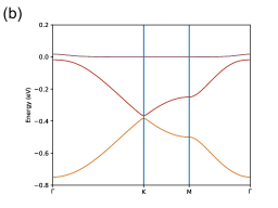
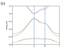
Figure 6: The evolution of the band structure of the (degenerate) $d_{xy}$ and $d_{x^{2}-y^{2}}$ orbitals along the $K-\Gamma-M-\Gamma$ in the first Brillouin zone for the tight-binding model Eq.(1) in the main text of the kagome metal-organic-framework with $E_{1}=E_{2}=2.0$eV, $E_{3}=1.0$eV, $V_{dd\pi}=V_{dd\delta}=V_{dd\sigma}=-0.25$eV in the spin up sector with a) $\lambda=0.0$eV, b) $\lambda=0.01$eV, and c) $\lambda=0.3$eV while $\lambda_{OS}=0.0,M_{z}=2.5,M_{x}=M_{y}=0.0$ all in eV. A “band inversion” phenomenon is visible.

We observe that the flat band gets inverted: for weak $\lambda$, the flat band is on top of two dispersive bands. However, for stronger $\lambda$ ($\gtrsim 0.3$eV in the example), the flat band falls below the dispersive bands. This can be viewed as a “band inversion” phenomenon. It is to be noted that for these two orbitals $d_{xy}$ and $d_{x^{2}-y^{2}}$, the spin-orbit coupling opens up a rather significant gap at both the Dirac point at $K$ and the quadratic band crossing at $\Gamma$, due to the fact that these orbitals have finite $m_{l}=\pm 2$.

Similar phenomenon of band inversion occurs to $d_{xz}$ and $d_{yz}$ orbitals. At weak spin-orbit coupling $\lambda$, the flat band occurs at the top while at strong $\lambda$, the flat band occurs at the bottom, as illustrated in Fig. 7. The gaps opened at Dirac and quadratic band crossing points are also reasonably significant, due to $m_{l}=\pm 1$.

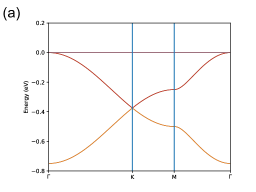
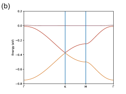
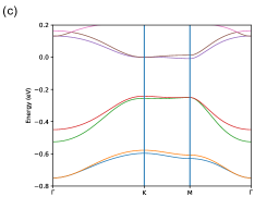
Figure 7: The evolution of the band structure of the (degenerate) $d_{xz}$ and $d_{yz}$ orbitals along the $K-\Gamma-M-\Gamma$ in the first Brillouin zone for the tight-binding model Eq.(1) in the main text of the kagome metal-organic-framework with $E_{1}=E_{3}=2.0$eV, $E_{2}=1.0$eV, $V_{dd\pi}=V_{dd\delta}=V_{dd\sigma}=-0.25$eV in the spin up sector with a) $\lambda=0.0$eV, b) $\lambda=0.01$eV, and c) $\lambda=0.4$eV while $\lambda_{OS}=0.0,M_{z}=2.5,M_{x}=M_{y}=0.0$ all in eV. A similar “band inversion” phenomenon is visible.

On the other hand, for the $d_{z^{2}}$ orbital, this band inversion phenomenon does not occur. In addition, because $m_{l}=0$ in this case, the Dirac point only acquires very small gap due to the $l_{x}s_{x}+l_{y}s_{y}$ term in the spin-orbit coupling. On the other hand, the quadratic brand crossing acquires a gap that is larger by one order of magnitude or more than that at the Dirac point, as illustrated in Fig. 8.

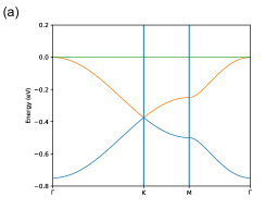
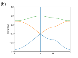
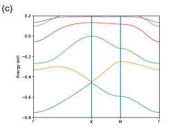
Figure 8: The evolution of the band structure of the (degenerate) $d_{z^{2}}$ orbital along the $K-\Gamma-M-\Gamma$ in the first Brillouin zone for the tight-binding model Eq.(1) in the main text of the kagome metal-organic-framework with $E_{1}=1.0$eV, $E_{2}=E_{3}=2.0$eV, $V_{dd\pi}=V_{dd\delta}=V_{dd\sigma}=-0.25$eV in the spin up sector with a) $\lambda=0.0$eV(with gapless Dirac point), b) $\lambda=0.3$eV(with extremely small gap at the Dirac point), and c) $\lambda=0.5$eV, while $\lambda_{OS}=0.0,M_{z}=2.5,M_{x}=M_{y}=0.0$ all in eV. No band inversion occurs. The Dirac point at $K$ acquires a very small gap while the quadratic band crossing at $\Gamma$ opens up a significant gap, as visible in c).

III Contribution of Different $d$-Orbitals to Quantum Anomalous Hall Effect

In this section, we elucidate the contribution of different $d$-orbitals to quantum anomalous Hall effect. Different $d$-orbitals contribute differently to the quantum anomalous Hall effect; some contribute significantly, the other do not contribute at all. To show this, we compute the Chern number that characterizes the quantum anomalous Hall effect by choosing the parameters appropriately in such a way that the contribution of each $d$-orbital can be isolated. For the sake of conciseness however, we assume degeneracy between symmetry-related orbitals; the $d_{xz}$ orbital is assumed to be degenerate with the $d_{yz}$ orbital while the $d_{xy}$ orbital is assumed to be degenerate with the $d_{x^{2}-y^{2}}$ orbital. When we identify the contribution of an orbital $d_{\alpha}$, we set the onsite energy of this orbital (and its degenerate partner) to be significantly lower than the remaining orbitals and we compute the Chern number in the Fermi energy range within the energy range of the orbital $d_{\alpha}$ under consideration.

The result of the calculation of Chern number $C$ vs Fermi energy $E_{F}$ from $d_{xz}$ and $d_{yz}$ orbitals is shown in Fig. 9. As can be seen, these orbitals do not display Chern plateaus even with rather strong spin-orbit coupling $\lambda=0.5$eV. In fact, the Chern peaks that they display as function of Fermi energy never exceed unity in absolute value, which cannot qualify them as nontrivial Chern number. Therefore, it can be concluded that these two orbitals do not contribute to the quantum anomalous Hall state.

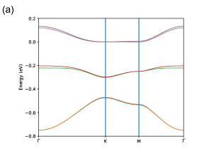
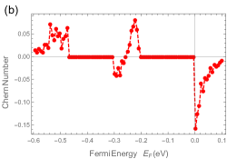
Figure 9: The a) band structure in the energy range corresponding to the $d_{xz}$ and $d_{yz}$ orbitals and b) the contribution of the $d_{xz}$ and $d_{yz}$ orbitals to the Chern number $C$ as a function of the Fermi energy $E_{F}$ (eV) at $T=0.0001$eV($\equiv 1.1$Kelvin) for the tight-binding model Eq.(1) in the main text of the kagome metal-organic-framework. To separate out these two $m_{l}=+/-1$ orbitals, we have set $E_{1}=E_{3}=2.0,E_{2}=1.0$eV, while using $V_{dd\pi}=V_{dd\delta}=V_{dd\sigma}=-0.25$eV, $\lambda_{OS}=0.0$eV, $M_{x}=M_{y}=0.0,M_{z}=2.5$eV with $\lambda=0.2$eV, where all five orbitals are included. The $C=0$ plateaus fall within the gaps of the $d_{xz}$ and $d_{yz}$ orbitals’ band structure.

The contribution of the $d_{xy}$ and $d_{x^{2}-y^{2}}$ orbitals on the Chern number vs Fermi energy is shown in Fig. 10. At realistic small values of spin-orbit coupling $\lambda\lesssim 0.3$eV, plateaus are visible, but with Chern number $C=0$. This suggests that these two orbitals have no contribution to quantum anomalous Hall effect in our system. As shown in Fig. 10 and discussed further in the next section, even a rather strong spin-orbit coupling $\lambda\gtrsim 0.5$eV gives plateaus with zero Chern number at Dirac point. The $d_{xy}$ and $d_{x^{2}-y^{2}}$ orbitals therefore do not give quantum anomalous Hall effect in our system.

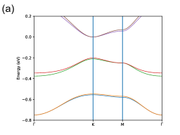
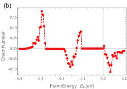
Figure 10: The a) band structure and b) contributions of the $d_{xy}$ and $d_{x^{2}-y^{2}}$ orbitals to the Chern number $C$ as a function of the Fermi energy $E_{F}$ (eV) at $T=0.0001$eV($\equiv 1.1$Kelvin) for the tight-binding model Eq.(1) in the main text of the kagome metal-organic-framework. To separate out these $m_{l}=+/-2$ orbitals, we have set $E_{1}=E_{2}=2.0$eV, $E_{3}=1.0$eV, while using $V_{dd\pi}=V_{dd\delta}=V_{dd\sigma}=-0.25$eV, $\lambda_{OS}=0.0$eV, $M_{x}=M_{y}=0.0,M_{z}=2.5$eV with $\lambda=0.2$eV where all five orbitals are included. Chern plateaus with $C=0$ appear within the band gaps: the one in the interval $(-0.2,0.0)$eV is from gapped Dirac point while the other in the interval $(-0.6,-0.4)$eV is from gapped quadratic band crossing point.

Finally, the Chern number contribution from $d_{z^{2}}$ orbital basically takes profile as shown in Fig. 5 in the main text. Two plateau peaks appear; one very sharp peak (i.e. very narrow plateau) at Dirac point and a broader plateau at DBC point.

IV Physical Origin of the Quantum Anomalous Hall Effect: The Effective Flux due to the Exchange-Type Spin-Orbit Coupling

In the previous sections, spin-orbit coupling was shown to have a strong influence on the band structure, the precise nature of which depends on each particular $d$ orbitals. In addition and therefore, the spin orbit-coupling also has strong influence on the Chern number contribution of each orbital, and therefore, its role in quantum anomalous Hall effect. We have also confirmed numerically that the absence of spin-orbit coupling (setting $\lambda=0$) gives zero Chern number, in agreement with the expectation that nonzero Chern number requires a gap within which the Fermi energy should fall.

As stated at the end of the previous section, for the $d_{z^{2}}$ orbital, the Chern plateau with $C=1$ appears in the presence of exchange-type spin-orbit coupling, at the gap associated with the QBC point at $\Gamma$ in the absence of spin-orbit coupling. As stressed in the main text, this $C=1$ QAHE can be interpreted as arising from the $\Phi=2\pi$ Berry phase of the QBC point, thus guaranteeing the stability and robustness of the $C=1$ Chern insulating state from the QBC point. The gapped Dirac point of the bands of the $d_{z^{2}}$ orbital also displays $C=1$ Chern plateau but with much narrower bandwidth, due to its much smaller gap.

On the other hand, the Chern number of Chern plateaus due to $d_{xy}$ and $d_{x^{2}-y^{2}}$ orbitals only give $C=0$ at any value of spin-orbit coupling, both at the gapped Dirac point and quadratic band crossing point, as illustrated in Fig.10. This demonstrates a completely different scenario for the realization of the QAHE compared to those known in existing literature, where the QAHE normally comes from the inter-orbital transition between $m_{l}=\pm 1$ $d$-orbitals ($d_{xz}$ and $d_{yz}$ orbitals) or between $m_{l}=\pm 2$ $d$-orbitals ($d_{xy}$ and $d_{x^{2}-y^{2}}$ orbitals) KontaniPRB2007SM  SCZhangPRL2015SM . This novel scenario is made possible by the geometry of the kagome lattice which involves triangles, which renders the hopping between nearest-neighbor sites to have both $x$ and $y$ components in general, allowing for contribution to transverse charge current even from $m_{l}=0$ $d$-orbital ($d_{z^{2}}$ orbital).

A theoretical explanation is provided as to why the gaps associated with the “non-trivial $d$-orbitals” do not contribute to the QAHE, giving $|C|=1$ as occurring in the kagome flux model  OhgushiPRBs . The key answer is that the flux pattern induced by the exchange-type spin-orbit coupling must be non-trivial; it must break time-reversal symmetry and therefore must be different from $0$ or $\pi$, while at the same time must satisfy the condition of zero net flux or zero average flux, as pointed out in the Haldane model  Haldane1988PRLs and satisfied also in the kagome flux model  OhgushiPRBs . This condition is not satisfied by the non-trivial orbitals in our model, as described in detail in the following.

Consider a triangle in a kagome lattice. The main contribution to the flux is provided by hopping between nearest-neighbor sites induced by the exchange-type spin-orbit coupling, combined with the complex phase factor provided by the overlap between $d$-orbitals of similar types; $d_{xz}-d_{yz}$ orbitals, and $d_{xy}-d_{x^{2}-y^{2}}$ orbitals. These pairs of $d$-orbitals give rise to the following complex factor for spin up electrons;

$$\langle d_{xz},s_{z}=+\frac{1}{2}|l_{z}|d_{yz},s_{z}=+\frac{1}{2}\rangle=-i,$$ (27)

$$\langle d_{yz},s_{z}=+\frac{1}{2}|l_{z}|d_{xz},s_{z}=+\frac{1}{2}\rangle=+i,$$ (28)

$$\langle d_{xy},s_{z}=+\frac{1}{2}|l_{z}|d_{x^{2}-y^{2}},s_{z}=+\frac{1}{2}\rangle=2i,$$ (29)

$$\langle d_{x^{2}-y^{2}},s_{z}=+\frac{1}{2}|l_{z}|d_{xy},s_{z}=+\frac{1}{2}\rangle=-2i,$$ (30)

where the bra and ket states are assumed to have the spin up state (the spin down state will give an additional minus sign to the right hand side of the equations). Several possible flux patterns induced by exchange-type spin-orbit coupling around a “down triangle” from clockwise hopping of $d$-orbital electrons in the kagome lattice within our model are illustrated in Fig.11. The flux factor associated with an arrow that goes from site $i$ to $j$ due to the exchange-type spin-orbit coupling arises from the overlap between the wave functions of the electrons from two $d$-orbital states; between the orbital $d_{\alpha}$ at site $i$ and the orbital $d_{\alpha^{\prime}}$ at site $j$. It can be seen that the net flux through the triangle is zero in all the patterns shown in Fig.11.

One can draw similar figures of flux pattern for the counter clockwise hopping of electron or the flux pattern for the “up triangle”. Finally, one can deduce the flux pattern for the hexagon, assuming a flux pattern where all down triangles have identical flux pattern among themselves and all up triangles have identical flux pattern among themselves. One will find that the flux through the hexagons is zero. One can also consider the overlap of these orbitals over the transverse part of the spin-orbit coupling; $\langle d_{\alpha},s_{z}|l_{x}s_{x}+l_{y}s_{y}|d_{\alpha^{\prime}},s^{\prime}_{z}\rangle$ where $\alpha,\alpha^{\prime}=xz,yz$ or $xy,x^{2}-y^{2}$ and $s_{z},s^{\prime}_{z}=\pm 1/2$. It is easy to see that the overlap is always zero.

It can therefore be concluded that the exchange-type spin-coupling gives zero flux at triangles and hexagons when only these “non-trivial” $d$-orbitals are involved. Despite having zero net flux, such trivial flux state does not have the flux structure needed to host a quantum Hall effect like that in the kagome flux model OhgushiPRBs . In fact, according to Haldane model, zero flux ($\phi=0$) gives $C=0$ from the gapped Dirac points. In other words, zero flux renders the paired Dirac points at $\pm K$ to always have gaps of the same sign. The exchange-type spin-orbit coupling in our model thus does not give rise to a QAHE from the Dirac points of the nonzero $m_{l}=\pm 1,\pm 2$ ($d_{xz},d_{yz},d_{xy},d_{x^{2}-y^{2}}$) $d$-orbitals in the band structure. This analysis explains the trivial Chern plateaus ($C=0$) observed in the figures of previous section coming from the nontrivial $d$-orbitals.

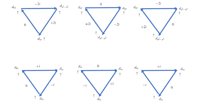
Figure 11: Several possible flux patterns in a “down triangle” of the kagome lattice due to the clockwise hopping of electrons with orbitals $d_{\alpha}(d_{\alpha^{\prime}})$ at site $i(j)$ respectively in the low energy (occupied) spin up sector, induced by the Ising part $l_{z}s_{z}$ of the exchange-type spin-orbit coupling (no spin flip during the hopping). The generally complex number $z_{ij}$ attached to each arrow pointing from site $i$ to site $j$ comes from the overlap factor $\langle d_{\alpha^{\prime}}|l_{z}|d_{\alpha^{\prime}}\rangle$ evaluated across the nearest-neighbor bond $\langle ij\rangle$. The arrow with 0 implies that the hopping is induced by the kinetic term rather than the spin-orbit coupling term. The flux $\phi$ is given by $\phi=\sum_{\langle ij\rangle}(\phi_{ij}+\pi/2)$ where the sum is around the loop traversing the triangle clockwise and the complex factor at each arrow is written as $iz_{ij}=|z_{ij}|\exp(i(\phi_{ij}+\pi/2))$ where the additional prefactor $i$ accounts for that in the last term of equation (1) in the main text. The net flux through the triangle is zero in all these patterns.

The non-vanishing contribution of the $d_{z^{2}}$ orbital to the quantum anomalous Hall effect (and its dominance, since all the other orbitals only give trivial $C=0$ plateaus) is made possible by the transverse part of the spin-orbit coupling $l_{x}s_{x}+l_{y}s_{y}$, which to our knowledge has not been considered by the existing works in the literature, which normally consider only the Ising part of the spin-orbit coupling $l_{z}s_{z}$ and which therefore omit the $d_{z^{2}}$ orbital because of its $m_{l}=0$. In fact, the $C=1$ Chern-insulating state can be explained by the same flux argument, but this time involving the overlaps of the $d_{z^{2}}$ orbital with all the other orbitals over the $l_{x}s_{x}+l_{y}s_{y}$ operator as given in the following

$$\langle d_{z^{2}},s_{z}=+\frac{1}{2}|l_{x}s_{x}+l_{y}s_{y}|d_{xz},s_{z}=-\frac{1}{2}\rangle=-\frac{\sqrt{3}}{2},$$ (31)

$$\langle d_{z^{2}},s_{z}=+\frac{1}{2}|l_{x}s_{x}+l_{y}s_{y}|d_{yz},s_{z}=-\frac{1}{2}\rangle=i\frac{\sqrt{3}}{2},$$ (32)

$$\langle d_{z^{2}},s_{z}=+\frac{1}{2}|l_{x}s_{x}+l_{y}s_{y}|d_{xy},s_{z}=-\frac{1}{2}\rangle=0,$$ (33)

$$\langle d_{z^{2}},s_{z}=+\frac{1}{2}|l_{x}s_{x}+l_{y}s_{y}|d_{x^{2}-y^{2}},s_{z}=-\frac{1}{2}\rangle=0,$$ (34)

while noting that

$$\langle d_{yz},s_{z}=+\frac{1}{2}|l_{x}s_{x}+l_{y}s_{y}|d_{xz},s_{z}=-\frac{1}{2}\rangle=\frac{i}{2}.$$ (35)

It is already clear from the flux factor involving the $d_{z^{2}}$ orbital in Eqs.(31-34) that considering a triangle where an electron hops between the sites of the triangle (while flipping its spin) in such a way that it takes the $d_{z^{2}}$ orbital state at one of the sites and $d_{xz}$ or $d_{yz}$ orbital states at the two other sites will give a nonzero net flux (that is, a phase factor $\exp(i\phi)$ to the electron wave function, where $\phi$ is the net flux through the triangle). The corresponding flux in the hexagon is $-2\phi$ so that the net (or average flux) is zero in the unit cell. This flux is the origin of the $C=1$ Chern insulating state due to the $d_{z^{2}}$ orbital, just like that in Haldane model  Haldane1988PRLs and kagome flux model  OhgushiPRBs . Examples of triangle with nonzero flux pattern are shown in Fig. 12.

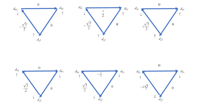
Figure 12: Several possible flux patterns in a “down triangle” of the kagome lattice due to the clockwise hopping of electrons with orbitals $d_{\alpha}(d_{\alpha^{\prime}})$ at site $i(j)$ respectively, induced by the transverse part $l_{x}s_{x}+l_{y}s_{y}$ of the exchange-type spin-orbit coupling (involving spin flip during the hopping).

Due to the topological character of the effective flux, it is independent of the strength of the spin-orbit coupling; the flux manifests once the spin-orbit coupling onset to nonzero value. The $C=1$ Chern plateau should thus be independent of the spin-orbit coupling; only its position in Fermi energy and width depends on the spin-orbit coupling $\lambda$. We have verified this numerically by computing the Chern plateau for two different values of spin-orbit coupling $\lambda$ while all other parameters are fixed.

V Contribution of On-site Spin-Orbit Coupling to Quantum Anomalous Hall Effect

The on-site spin-orbit interaction in our pure $d$-electron model is unable to generate any quantum anomalous Hall effect; the topological invariant is practically zero at all energies, regardless of the strength of the on-site spin-orbit interaction. Different from existing works where onsite spin-orbit coupling in tight-binding models on a square lattice with $s$-orbital and $d$-orbital electrons  KontaniJPSJ762007 or with $d$-orbital electrons but with second-neighbor hopping  KontaniPRL2008 drives other types of Hall effect due the resulting flux structure, in our pure $d$-orbital system, the onsite spin-orbit coupling does not generate the flux structure necessary to give a QAHE. The band structure simply involves a vertical shift of the bands of different orbitals, giving no nontrivial gap (neither at Dirac nor at quadratic band crossing points) necessary for a Chern insulating state. For onsite spin-orbit coupling to generate the anomalous Hall effect, coupling to orbitals with different $l$ (e.g. $s$ orbital; i.e. $l=0$) is necessary  KontaniJPSJ762007 , but this is not pertinent to a kagome metal where the physics is entirely dominated by $d$-orbital electrons.

Within a tight-binding model, spin-orbit coupling is normally written as coupling between the spin and orbital angular momentum carried by the electron hopping between nearest or next-neighbor sites. Intuitively, such hopping spin-orbit coupling term effectively corresponds to a flux or complex phase factor acquired by the electron wave function when traversing a closed trajectory as it hops between the sites of the lattice. However, one can also consider a local spin-orbit interaction, coupling the spin of electron and its local angular momentum defined on each site, as represented by the fourth term in Eq.(1) in the main text. The onsite spin-orbit coupling corresponds to spin-dependent uniform magnetic field in real space and induces Landau level-type of gaps, shifting bands of different orbitals away from each other, as illustrated in Fig. 13. Such effective field does not open up gap at the Dirac point, nor at the quadratic gapless point. In fact, other than the Zeeman field gap due to $M_{z}$, the band structure contains no nontrivial gap as the bands of each spin sector still overlap with each other, at least for realistic small spin-orbit coupling $\lambda_{OS}\lesssim 0.5$eV. As a result, the Chern number is practically zero and there is no quantum anomalous Hall effect due to onsite spin-orbit coupling, as confirmed in Fig. 14.

It will be explained here why our model does not accommodate QAHE from onsite spin-orbit coupling, using flux argument, following existing works  OhgushiPRBs  KontaniJPSJ762007  KontaniPRL2008 . Consider a triangle in a kagome lattice. The main contribution to the flux is provided by hopping between nearest-neighbor sites, combined with the complex phase factor provided by the overlap between $d$-orbitals of similar types; $d_{xz}-d_{yz}$ orbitals, and $d_{xy}-d_{x^{2}-y^{2}}$ orbitals. These pairs of $d$-orbitals give rise to the same complex factor for spin up electrons, as given in Eqs.(27-30), except that the overlap occurs at the site $j$ after the electron hops from the site $i$ to $j$.

The resulting flux patterns are similar to those arising due to exchange-type spin-orbit coupling, as illustrated in Fig. 15. The flux factor associated with an arrow that goes from site $i$ to $j$ is that due to onsite spin-orbit coupling at $j$ from two $d$-orbital states; between the orbital $d_{\alpha}$ at site $i$ and the orbital $d_{\alpha^{\prime}}$ at site $j$. It can be seen that the net flux factor is zero in all the patterns shown in Fig. 15.

Analogous figures of flux pattern for the “up triangle” can be easily constructed in similar way as those for the down triangles. Considering the flux pattern at up and down triangles, one can deduce the flux pattern for the hexagon, assuming a flux pattern where all down triangles have identical flux pattern among themselves and all up triangles have identical flux pattern among themselves. As in the exchange-type spin-orbit coupling case, the flux through the hexagons is also zero. It can therefore be concluded that the onsite spin-coupling gives zero flux at triangles and hexagons. By comparison with the kagome flux phase that hosts a quantum Hall effect  OhgushiPRBs , the onsite spin-orbit coupling in our model thus does not give rise to a QAHE.

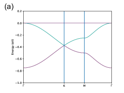
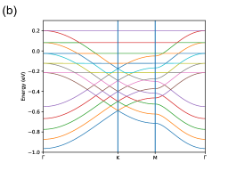
Figure 13: The band structure along the $K-\Gamma-M-\Gamma$ in the first Brillouin zone for the tight-binding model Eq.(1) in the main text of the kagome metal-organic-framework with $E_{1}=E_{2}=E_{3}=1.0$eV, $V_{dd\pi}=V_{dd\delta}=V_{dd\sigma}=-0.25$eV in the spin up sector with a) $\lambda_{OS}=0.0$eV and b) $\lambda_{OS}=0.2$eV, while $\lambda=0.0,M_{z}=2.5,M_{x}=M_{y}=0.0$ all in eV. This figure indicates that onsite spin-orbit coupling simply splits the bands vertically away from each other, without opening gap at Dirac point or quadratic band crossing.

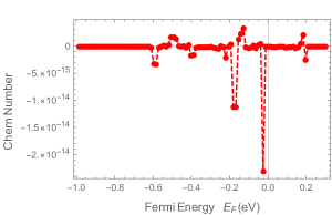
Figure 14: The Chern number $C$ as a function of the Fermi energy $E_{F}$ (eV) evaluated at $T=0.0001$eV($\equiv 1.1$Kelvin) for the tight-binding model Eq.(1) in the main text of the kagome metal-organic-framework with $E_{1}=E_{2}=E_{3}=1.0$eV, while $V_{dd\pi}=V_{dd\delta}=V_{dd\sigma}=-0.25$eV, $\lambda=0.0$eV, $M_{x}=M_{y}=0.0,M_{z}=2.5$eV but with $\lambda_{OS}=0.2$eV, where all five orbitals are included. Despite the spiky profile, the Chern number is effectively zero.

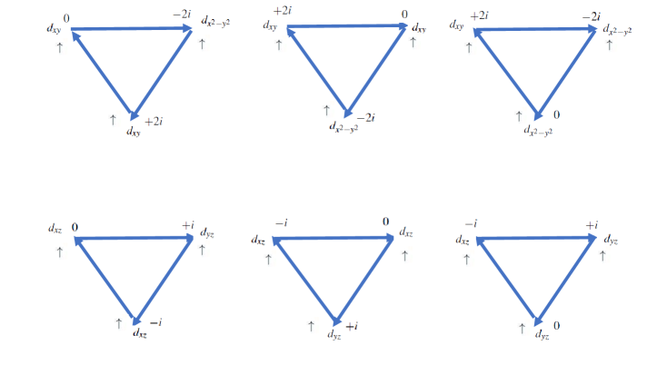
Figure 15: The flux pattern in a “down triangle” of the kagome lattice due to the (Ising part of) onsite spin-orbit coupling and nearest-neighbor hopping of electrons with orbitals $d_{\alpha}(d_{\alpha^{\prime}})$ at site $i(j)$ respectively in the low energy (occupied) spin up sector. The generally complex number attached to the end of each arrow pointing from site $i$ to site $j$ comes from the overlap factor $\langle d_{\alpha^{\prime}}|l_{z}|d_{\alpha^{\prime}}\rangle$ evaluated at site $j$. Different from the flux patterns in Figs.11 and 12, here the hopping between sites, as marked by the arrow, is induced by the kinetic hopping term, $t_{ij;\alpha\alpha^{\prime}}$ which is non-directional; no sign change when the arrow is reversed. As such, the hopping does not induce the flux needed to open up a gap, and hence no QAHE.

References

- (1) N. Nagaosa, J. Sinova, S. Onoda, A. H. MacDonald, and N. P. Ong, Rev. Mod. Phys. 82, 1539 (2010).
- (2) R. Karplus and J. M. Luttinger, Phys. Rev. 95, 1154 (1954).
- (3) J. Smit, Physica (Amsterdam) 21, 877 (1955).
- (4) J. M. Luttinger, Phys. Rev. 112, 739 (1958).
- (5) J. Kondo, Prog. Theor. Phys. 27, 772 (1962).
- (6) L. Berger, Phys. Rev. B 2, 4559 (1970).
- (7) P. Nozieres and C. Lewiner, J. Phys. (Paris) 34, 901 (1973).
- (8) T. Jungwirth, Qian Niu, and A. H. MacDonald, Phys. Rev. Lett. 88, 207208 (2002).
- (9) M. Onoda and N. Nogaosa, J. Phys. Soc. Jpn. 71, 19 (2002).
- (10) H. Kontani, T. Tanaka, and K. Yamada, Phys. Rev. B 75, 184416 (2007).
- (11) T. Neupert, L. Santos, C. Chamon, and C. Mudry, Phys. Rev. Lett. 106, 236804 (2011).
- (12) K. Sun, Z. Gu, H. Katsura, and S. Das Sarma Phys. Rev. Lett. 106, 236803 (2011).
- (13) E. Tang, J-W. Mei, and X-G. Wen, Phys. Rev. Lett. 106, 236802 (2011).
- (14) M. Kang, L. Ye, S. Fang, J-S. You, A. Levitan, M. Han, J. I. Facio, C. Jozwiak, A. Bostwick, E. Rotenberg, M. K. Chan, R. D. McDonald, D. Graf, K. Kaznatcheev, E. Vescovo, D. C. Bell, E. Kaxiras, J. van den Brink, M. Richter, M. P. Ghimire, J. G. Checkelsky, and R. Comin, Nature Materials, 19, 163-169 (2020).
- (15) R. Zhang, J. Liu, Y. Gao, M. Hua, B. Xia, P. Knecht, A. C. Papageorgiou, J. Reichert, J. V Barth, H. Xu, L. Huang, and N. Lin, Angew. Chem. Int. Ed. 10, 13698 (2019).
- (16) M. Hua, B. Xia, M. Wang, E. Li, J. Liu, T. Wu, Y. Wang, R. Li, H. Ding, J. Hu, Y. Wang, J. Zhu, H. Xu, W. Zhao, and N. Lin, J. Phys. Chem. Lett. 12, 3733 (2021).
- (17) N. Shaiek, H. Denawi, M. Koudia, R. Hayn, S. Schäfer, I. Berbezier, C. Lamine, O. Siri, A. Akremi, and M. Abel, Advanced Materials Interfaces 9, 2201099 (2022).
- (18) A. H. Denawi, X. Bouju, M. Abel, J. Richter, and R. Hayn, Phys. Rev. Materials 7, 074201 (2023).
- (19) I. Makhfudz, Phys. Rev. B 89, 024401 (2014).
- (20) L. Savary and L. Balents, Rep. Prog. Phys. 80, 016502 (2017).
- (21) S. Nishimoto, N. Shibata, and C. Hotta, Nat. Commun. 4, 2287 (2013).
- (22) S. Capponi, O. Derzhko, A. Honecker, A. M. Läuchli, and J. Richter, Phys. Rev. B 88, 144416 (2013).
- (23) I. Makhfudz and P. Pujol, Phys. Rev. Lett. 114, 087204 (2015).
- (24) Taguchi Y, Oohara Y, Yoshizawa H, Nagaosa N, and Tokura Y., Science 291(5513), 2573 (2001).
- (25) J. Ye, Y. B. Kim, A. J. Millis, B. I. Shraiman, P. Majumdar, and Z. Tešanović, Phys. Rev. Lett. 83, 3737 (1999).
- (26) S. Onoda and N. Nagaosa, Phys. Rev. Lett. 90, 196602 (2003).
- (27) I. Martin and C. D. Batista, Phys. Rev. Lett. 101, 156402 (2008).
- (28) Ohgushi K., Murakami S., Nagaosa N., Phys. Rev. B 62, R6065 (2000).
- (29) Z. Fang, N. Nagaosa, K. S. Takahashi, A. Asamitsu, R. Mathieu, T. Ogasawara, H. Yamada, M. Kawasaki, Y. Tokura, and K. Terakura, Science 302, 92 (2003).
- (30) M. Taillefumier, B. Canals, C. Lacroix, V. K. Dugaev, and P. Bruno Phys. Rev. B 74, 085105 (2006).
- (31) H. Chen, Q. Niu, and A. H. MacDonald, Phys. Rev. Lett. 112, 017205 (2014).
- (32) P. Bruno, V. K. Dugaev, and M. Taillefumier, Phys. Rev. Lett. 93, 096806 (2004).
- (33) I. Makhfudz and P. Pujol, Phys. Rev. B 92, 144507 (2015).
- (34) G. Sundaram and Q. Niu, Phys. Rev. B 59, 14 915 (1999).
- (35) N. A. Sinitsyn, J. Phys.; Cond. Matt. 20 (2008) 023201.
- (36) F. D. M. Haldane, Phys. Rev. Lett. 93, 206602 (2004).
- (37) D. J. Thouless, M. Kohmoto, M. P. Nightingale, and M. den Nijs, Phys. Rev. Lett. 49, 405 (1982).
- (38) C-Z. Chang, C-X. Liu, and A. H. MacDonald, Rev. Mod. Phys. 95, 011002 (2023).
- (39) F. D. M. Haldane, Phys. Rev. Lett. 61, 2015 (1988).
- (40) M. Onoda and N. Nagaosa, Phys. Rev. Lett. 90, 206601 (2003).
- (41) K. Sun, H. Yao, E. Fradkin, and S. A. Kivelson, Phys. Rev. Lett. 103, 046811 (2009).
- (42) Z.Qiao, W. Ren, H. Chen, L. Bellaiche, Z. Zhang, A. H. MacDonald, and Q. Niu, Phys. Rev. Lett. 112, 116404 (2014).
- (43) P. Högl, T. Frank, K. Zollner, D. Kochan, M. Gmitra, and J. Fabian, Phys. Rev. Lett. 124, 136403 (2020).
- (44) C-X. Liu, X-L. Qi, X. Dai, Z. Fang, and S-C. Zhang, Phys. Rev. Lett. 101, 146802 (2008).
- (45) C-X. Liu, S-C. Zhang, and X-L. Qi, Annu. Rev. Condens. Matter Phys. 7, 301 (2016).
- (46) C-Z. Chang, J. Zhang, X. Feng, J. Shen, Z. Zhang, M. Guo, K. Li, Y. Ou, P. Wei, L-L. Wang, Z-Q. Ji, Y. Feng, S. Ji, X. Chen, J. Jia, X. Dai, Z. Fang, S-C. Zhang, K. He, Y. Wang, L. Lu, X-C. Ma, and Q-K. Xue, Science 340, 167 (2013).
- (47) Deng, Y., Yu, Y., Shi, M. Z., Guo, Z., Xu, Z., Wang, J., Chen, X. H., and Zhang, Y., Science 367, 895 (2020).
- (48) H. Huang, Z. Liu, H. Zhang, W. Duan, and D. Vanderbilt, Phys. Rev. B 92, 161115(R)(2015).
- (49) Z. F. Wang, Z. Liu, and F. Liu, Phys. Rev. Lett. 110, 196801 (2013).
- (50) Z. Liu, Z-F. Wang, J-W. Mei, Y-S. Wu, and F. Liu, Phys. Rev. Lett. 110, 106804 (2013).
- (51) S. Baidya, S. Kang, C. H. Kim, and J. Yu, Scientific Reports 9, 13807 (2019).
- (52) G. Xu, B. Lian, and S-C. Zhang, Phys. Rev. Lett. 115, 186802 (2015).
- (53) L. Ye, M. Kang, J. Liu, F. von Cube, C. R. Wicker, T. Suzuki, C. Jozwiak, A. Bostwick, E. Rotenberg, D. C. Bell, L. Fu, R. Comin, and J. G. Checkelsky, Nature 555, 638 (2018).
- (54) W. A. Harrison, Electronic Structure and the Properties of Solids: The Physics of the Chemical Bond (Dover Publications, Inc., New York, United States (1980)).
- (55) Please see the supplementary materials containing, among others, the diagonalization of the Hamiltonian including the details of Slater-Koster integrals, the evolution of the band structures of the -orbitals with , the computed Chern number vs. Fermi energy and its dependencies on various parameters, the effective flux analysis, and the role of spin-orbit coupling. These materials also make reference to AHErmp KontaniPRB2007 Denawi OhgushiPRB Haldane1988PRL SCZhangPRL Harrison Fukui KontaniJPSJ762007main KontaniPRL2008main .
- (56) C. L. Kane and E. J. Mele, Phys. Rev. Lett. 95, 226801 (2005).
- (57) As discussed in SupplementaryMaterials , the onsite spin-orbit coupling turns out to be complementary; i.e. unable to produce any QAHE, and is thus set to zero for simplicity. The in-plane magnetization is also set to zero as we assume magnetization perpendicular to the plane.
- (58) T. Fukui, Y. Hatsugai, and H. Suzuki, J. Phys. Soc. Jpn. 74, 61675 (2005).
- (59) H. Kontani, M. Naito, D. S. Hirashima, K. Yamada, and J. Inoue, J. Phys. Soc. Jpn. 76, 103702 (2007).
- (60) H. Kontani, T. Tanaka, D. S. Hirashima, K. Yamada, and J. Inoue, Phys. Rev. Lett. 100, 096601 (2008).

References

- (1) W. A. Harrison, Electronic Structure and the Properties of Solids: The Physics of the Chemical Bond (Dover Publications, Inc., New York (1980)).
- (2) N. Nagaosa, J. Sinova, S. Onoda, A. H. MacDonald, and N. P. Ong, Rev. Mod. Phys. 82, 1539 (2010).
- (3) T. Fukui, Y. Hatsugai, and H. Suzuki, J. Phys. Soc. Jpn. 74, 61675 (2005).
- (4) F. D. M. Haldane, Phys. Rev. Lett. 61, 2015 (1988).
- (5) Ohgushi K., Murakami S., Nagaosa N., Phys. Rev. B 62, R6065 (2000).
- (6) A. H. Denawi, X. Bouju, M. Abel, J. Richter, and R. Hayn, Phys. Rev. Materials 7, 074201 (2023).
- (7) H. Kontani, T. Tanaka, and K. Yamada, Phys. Rev. B 75, 184416 (2007).
- (8) G. Xu, B. Lian, and S-C. Zhang, Phys. Rev. Lett. 115, 186802 (2015).
- (9) H. Kontani, M. Naito, D. S. Hirashima, K. Yamada, and J. Inoue, J. Phys. Soc. Jpn. 76, 103702 (2007).
- (10) H. Kontani, T. Tanaka, D. S. Hirashima, K. Yamada, and J. Inoue, Phys. Rev. Lett. 100, 096601 (2008).