Fluid and kinetic studies of tokamak disruptions using Bayesian optimization

Abstract

When simulating runaway electron dynamics in tokamak disruptions, fluid models with lower numerical cost are often preferred to more accurate kinetic models. The aim of this work is to compare fluid and kinetic simulations of a large variety of different disruption scenarios in ITER. We consider both non-activated and activated scenarios; for the latter we derive and implement kinetic sources for the Compton scattering and tritium beta decay runaway electron generation mechanisms in our simulation tool Dream [M. Hoppe et al 2021 Comp. Phys. Commun. 268, 108098]. To achieve a diverse set of disruption scenarios, Bayesian optimization is utilized to explore a range of massive material injection densities for deuterium and neon. The cost function is designed to distinguish between successful and unsuccessful disruption mitigation based on the runaway current, current quench time and transported fraction of the heat loss. In the non-activated scenarios, we find that fluid and kinetic disruption simulations can have significantly different runaway electron dynamics, due to an overestimation of the hot-tail generation rate by the fluid model. The primary cause of this is that the fluid hot-tail generation model neglects superthermal electron transport losses during the thermal quench. In the activated scenarios the fluid and kinetic models give similar predictions, which can be explained by the activated sources’ significant influence on the RE dynamics and the seed.

1 Introduction

Plasma-terminating disruptions are one of the main challenges facing tokamak fusion reactors. Disruptions are off-normal events, leading to a sudden cooling of the plasma – a thermal quench (TQ) – associated with an increase in the plasma resistivity, causing the plasma current to decay over the longer current quench (CQ). The toroidal current cannot change significantly on the short TQ timescale, and therefore an inductive electric field is produced, which can accelerate electrons to relativistic energies (Helander et al., 2002; Breizman et al., 2019). There are several problems associated with disruptions, including heat loads on the plasma facing components and mechanical stresses due to electromagnetic forces (Hollmann et al., 2015). One of the most significant problems, however, is the generation of highly energetic runaway electron (RE) beams.

Runaway generation is expected to be a major problem in the next generation of machines with high plasma currents, such as ITER (Hender et al., 2007). The reason is that avalanche multiplication of seed REs is exponentially sensitive to the initial plasma current (Rosenbluth & Putvinski, 1997). In addition, during deuterium-tritium operation, REs can also be generated by Compton scattering of $\gamma$ photons and tritium beta decay. These activated generation sources will represent two irreducible sources of energetic electrons and are therefore expected to be the dominant RE seed generation mechanisms in future reactor-scale tokamaks when hot-tail and Dreicer generation have been successfully mitigated. An uncontrolled, localized loss of a relativistic runaway beam may result in damage to the first wall. One of the most prominent mitigation methods is massive material injection (MMI) of a combination of radiating impurities (e.g. neon) and hydrogen isotopes, either in gaseous or solid state. Shattered pellet injection is the reference concept for the disruption mitigation system in ITER. However, as of yet, the problem of designing a successful disruption mitigation strategy is still unsolved.

Several sophisticated simulation codes have been developed in order to study disruptions. One such code is Dream (Hoppe et al., 2021a), that is primarily developed for the study of REs. Dream has several options for simulating electron dynamics – ranging from fluid to fully kinetic models. Dream has already been used to study several aspects of tokamak disruption mitigation – including finding parameter spaces without REs for SPARC (Tinguely et al., 2021; Izzo et al., 2022; Tinguely et al., 2023), STEP (Berger et al., 2022) and ITER (Pusztai et al., 2023). These studies used RE fluid models, i.e. the momentum-space runaway dynamics is replaced by formulas for the steady-state runaway generation rates as functions of the background parameters.

Kinetic plasma models are physically more rigorous, and can in certain scenarios yield significantly different results compared to those obtained from fluid models. In kinetic models, the Dreicer and hot-tail RE generation mechanisms are naturally included because the dynamics in the electron velocity space is modelled by the Fokker-Planck collision operator. In certain cases, there may be substantial discrepancies between the kinetic and fluid generation rates. For example, in Dream, the hot-tail generation mechanism is implemented as a generation rate based on a simplified model (Smith & Verwichte, 2008), which is derived under the assumption that there are no magnetic perturbations. This model can significantly overestimate the RE generation rate when magnetic perturbations are present.

Pusztai et al. (2023) used the fluid RE model in Dream to explore the injected density space of MMI, with Bayesian optimization, to investigate scenarios for disruption mitigation in ITER. However, such a comprehensive exploration of the parameter space has not been performed using kinetic modelling. Even though isolated studies using kinetic models have been done (Vallhagen et al., 2022; Svenningsson et al., 2021), a thorough exploration of the MMI injected density space would not be feasible for a fully kinetic model, due to the many simulations needed combined with the high computational cost of fully kinetic simulations. Using an isotropic kinetic model for such exploration is however feasible, i.e. the model which evolves a distribution function which is analytically averaged over pitch angle. Such procedure is justified for the mildly superthermal region where the complicated hot-tail dynamics takes place, while the relativistic electrons can again be treated in a simplified manner. The isotropic kinetic model in Dream is several orders of magnitude faster than the corresponding fully kinetic model (Hoppe et al., 2021a).

The aim of this article is to compare fluid and kinetic disruption simulations for an ITER-like disruption scenario. We explore the injected density space of MMI, utilizing Bayesian optimization for sample selection. We start by deriving kinetic expressions for the RE generation sources from tritium beta decay and Compton scattering (section 2). Then we proceed by constructing an informative cost function (section 3.2) for efficient sample selection during the Bayesian optimization (section 3).

Our results show that in the non-activated scenarios, the fluid and kinetic models yield significantly different optima (section 4). This can be explained mainly by the hot-tail generation rate being overestimated when using the fluid model. In the activated scenarios, the fluid and kinetic models yield more similar results. In these cases, the Compton generation mechanism is dominant, which is well represented in the fluid model.

2 Kinetic runaway electron generation sources

Runaway electron generation is an inherently kinetic process, as it depends on details in the velocity distribution function that are determined by a balance between collisional friction, electric-field acceleration and radiation processes. With the kinetic models in Dream, the generation of REs from the Dreicer and hot-tail mechanisms is included in the dynamics modelled by the Fokker-Planck collision operator, while REs generated via avalanche multiplication are accounted for using a semi-analytical growth rate by Hesslow et al. (2019a) which has been benchmarked against kinetic simulations.

The activated generation processes, Compton scattering and tritium beta decay, provide energetic electrons that are continually generated over a range of electron velocities. Under the assumption that these generation mechanisms are isotropic in velocity space, kinetic sources can be derived using the same reasoning as for their fluid counterparts (Martín-Solís et al., 2017). For tritium beta decay, this assumption is justified since the emission angle of electrons during this process is random and uniformly distributed. For Compton scattering, gamma photons will be emitted from the walls and enter the plasma from all sides in a nearly isotropic manner, even traversing walls, because the plasma is optically thin to the photons. Therefore the resulting electron distribution can be assumed to be approximately uncorrelated with the pitch angle.

2.1 Tritium beta decay

The kinetic source rate due to tritium decay rate $(\differential f/\differential t)_{T}$ can be derived using the expression for the energy spectrum of electrons emitted through beta decay (Krane, 1988)

$$f_{\beta}(W)\propto F(p,2)p\mathcal{W}(W_{\rm max}-W)^{2}\quad\text{for }W\leq W_{\rm max}\text{, and }f_{\beta}(W)=0\text{ above}\;W_{\rm max}.$$ (1)

Here $\mathcal{W}={m_{\rm e}}c^{2}\gamma$ is the total energy, $W={m_{\rm e}}c^{2}(\gamma-1)$ is the kinetic energy, $\gamma=\sqrt{p^{2}+1}$ is the Lorentz factor and $p$ is the momentum normalized to ${m_{\rm e}}c$. Since the maximum energy of the emitted electrons is $W_{\rm max}=$18.6\text{\,}\mathrm{k}\mathrm{e}\mathrm{V}$\ll{m_{\rm e}}c^{2}$, we may take the non-relativistic limit of the Fermi function (Fermi, 1934),

$$F(p,Z_{\rm f})=\frac{2\pi\alpha Z_{\rm f}/\beta}{1-\exp(-2\pi\alpha Z_{\rm f}/\beta)},$$ (2)

with the normalized speed $\beta=p/\gamma$, the charge of the final state nucleus $Z_{\rm f}$ (for tritium decay $Z_{\rm f}=2$), and the fine structure constant $\alpha\approx 1/137$.

Since the source is isotropic we may write

$$4\pi p^{2}\differential p\left(\derivative{f}{t}\right)_{\rm T}=\differential Wf_{\beta}(W).$$ (3)

Using $\differential W/\differential p={m_{\rm e}}c^{2}\beta$ we find

$$\left(\derivative{f}{t}\right)_{\rm T}=\frac{1}{4\pi p^{2}}f_{\beta}(W){m_{\rm e}}c^{2}\beta\propto\frac{1}{p^{2}}\frac{p\gamma(\gamma_{\rm max}-\gamma)^{2}}{1-\exp[-4\pi\alpha/\beta]}.$$ (4)

The requirement that the source integrated over the entire momentum space yields the tritium decay rate, $(\ln 2)\,n_{\rm T}/\tau_{\rm T}$ – where $\tau_{\rm T}\approx 4500$ days is the half-life for tritium – determines the proportionality factor in (4) such that

$$\left(\derivative{f}{t}\right)_{\rm T}\approx C\frac{\ln 2}{4\pi}\frac{n_{\rm T}}{\tau_{\rm T}}\frac{1}{p^{2}}\frac{p\gamma\left(\gamma_{\rm max}-\gamma\right)^{2}}{1-\exp(-4\pi\alpha/\beta)},$$ (5)

with the constant

$$C=1\left/\int_{0}^{p_{\rm max}}\frac{1}{p^{2}}\frac{p\gamma\left(\gamma_{\rm max}-\gamma\right)^{2}}{1-\exp(-4\pi\alpha/\beta)}p^{2}\differential p\right.\approx 31800,$$ (6)

where $p_{\rm max}$ is the momentum corresponding to $W_{\rm max}$.

2.2 Compton scattering rate

The kinetic Compton scattering rate can be calculated using the Compton cross-section and the gamma energy flux spectrum emitted by a given wall material. When utilizing the kinematic relation between the photon energy $W_{\gamma}$, and the energy $W$ and deflection angle $\theta$ of the scattered electron, we can write

$$\cos\theta=1-\frac{{m_{\rm e}}c^{2}}{W_{\gamma}}\frac{W}{W_{\gamma}^{\prime}},$$ (7)

where $W_{\gamma}^{\prime}=W_{\gamma}-W$ is the scattered photon energy. The Compton scattering process is described by the Klein-Nishina differential cross-section

$$\derivative{\sigma}{\Omega}=\frac{r_{\rm e}^{2}}{2}\frac{W_{\gamma}^{\prime 2}}{W_{\gamma}^{2}}\left[\frac{W_{\gamma}}{W_{\gamma}^{\prime}}+\frac{W_{\gamma}^{\prime}}{W_{\gamma}}-\sin^{2}(\theta)\right],$$ (8)

with $r_{\rm e}=e^{2}/4\pi\varepsilon_{0}m_{\rm e}c^{2}$ being the classical electron radius.

Thus, in a plasma with the total electron density $n_{\rm e,tot}$ and isotropic photon distribution, we can write

$$4\pi p^{2}\differential p\left(\derivative{f}{t}\right)_{\rm C}=n_{\rm e,tot}\int_{W_{\gamma 0}}^{\infty}\differential W_{\gamma}\left[\Gamma_{\gamma}(W_{\gamma})\left(2\pi\sin\theta\derivative{\sigma}{\Omega}\right)\differential\theta(W,W_{\gamma})\right],$$ (9)

where $\Gamma_{\gamma}(W_{\gamma})$ is the gamma energy flux spectrum. The lower integration limit $W_{\gamma 0}$ can be derived from equation (7) as $W_{\gamma 0}=(p+\gamma-1)/2$.

Martín-Solís et al. (2017) estimated the photon flux energy spectrum in ITER by $\Gamma_{\gamma}(W_{\gamma})=\Gamma_{0}\exp[-\exp(-z)-z+1]$, where ${z=[\ln(W_{\gamma}/10^{6})+1.2]/0.8}$ and

$$\Gamma_{0}=\Gamma_{\rm flux}\displaystyle\left/\int_{0}^{\infty}\exp[-\exp(-z)-z+1]\,\differential W_{\gamma}\right.=\Gamma_{\rm flux}/5.8844,$$ (10)

with the total flux ${\Gamma_{\rm flux}=10^{18}}/(\rm m^{2}s)$. The runaway production rate from Compton scattering can be obtained as

$$\left(\derivative{f}{t}\right)_{\rm C} =\frac{n_{\rm e,tot}}{2}\frac{1}{p^{2}}\int_{W_{\gamma 0}}^{\infty}\differential W_{\gamma}\Gamma_{\gamma}(W_{\gamma})\sin\theta\derivative{\sigma}{\Omega}\derivative{\theta}{p}$$ (11a)

$$=\frac{n_{\rm e,tot}}{2}\frac{1}{p^{2}}\int_{W_{\gamma 0}}^{\infty}\differential W_{\gamma}\Gamma_{\gamma}(W_{\gamma})\derivative{\sigma}{\Omega}\frac{\beta}{\left(\frac{W_{\gamma}}{{m_{\rm e}}c^{2}}+1-\gamma\right)^{2}},$$ (11b)

where we have used

$$\derivative{\theta}{p}=\derivative{p}\arccos\left(1-\frac{{m_{\rm e}}c^{2}/W_{\gamma}}{\frac{W_{\gamma}}{{m_{\rm e}}c^{2}(\gamma-1)}-1}\right)=\frac{p/\gamma}{\sqrt{1-\cos^{2}\theta}\left(\gamma-1\right)^{2}\left(\frac{W_{\gamma}/{m_{\rm e}}c^{2}}{\gamma-1}-1\right)^{2}}.$$ (12)

Both the kinetic tritium and Compton sources are consistent with the fluid runaway generation rate (Martín-Solís et al., 2017)

$$\left(\derivative{n_{\rm re}}{t}\right)_{\rm T/C}=\int_{p>p_{\rm c}}\differential^{3}\boldsymbol{p}\left(\derivative{f}{t}\right)_{\rm T/C},$$ (13)

when the runaway region is set to be above the critical momentum for RE generation $p_{\rm c}$.

3 Bayesian optimization of simulated disruptions

In this paper we will compare disruption simulations using an isotropic reduced kinetic model, described in Appendix B.2 of (Hoppe et al., 2021a), and a computationally less expensive fluid model. The comparison of fluid and kinetic simulations for a wide variety of disruption scenarios was facilitated using Bayesian optimization. The disruption model and simulation details used are described in section 3.1, while the Bayesian optimization is detailed in section 3.3. In section 3.2, the design and motivation of the cost function is presented.

3.1 Simulation setup

The simulations are performed using the numerical tool Dream  (Disruption Runaway Electron Analysis Model). Dream simulates the plasma evolution of tokamak disruptions self-consistently, including the evolution of the plasma temperature, current densities, electron and ion densities, ion charge states and electric field. The simulations are performed with a multi-fluid plasma model, with the possibility of simulating some, or all, subsets of the total electron population kinetically. Dream divides the electrons into up to three populations.

Both in the fluid and the kinetic simulations performed here, the bulk and RE populations are treated as distinct fluids. The bulk electrons are characterized by their density ${n_{\rm e}}$, temperature ${T_{\rm e}}$ and the Ohmic current density ${j_{\Omega}}$. The REs are described by their density ${n_{\rm re}}$, which also yields the runaway current density ${j_{\rm re}}=ec{n_{\rm re}}$, because they are assumed to move with the speed of light parallel to the magnetic field. The total current density ${j_{\Omega}}+{j_{\rm re}}$ is governed by the evolution of the poloidal flux $\psi(r)$ (Hoppe et al., 2021a). For the electrical conductivity $\sigma$ which enters in this evolution, we use the model described by Redl et al. (2021), that is valid for arbitrary plasma shaping and collisionality and takes into account the effects of trapping.

In the kinetic simulations there is an additional population of superthermal electrons that are represented by the distribution function ${f_{\rm hot}}$, which is evolved using a pitch-angle averaged Fokker–Planck equation (Hoppe et al., 2021a). This division of the hot and cold populations is especially suitable when there are two distinct Maxwellian electron populations present in the plasma, as is the case when cold materials are injected into a hot plasma during massive material injection.

The temperature of the cold population is determined by a time dependent energy balance equation, accounting for Ohmic heating, line and recombination radiation and bremsstrahlung, as well as a radial heat transport, according to equation (43) of (Hoppe et al., 2021a). The ionization, recombination and radiation rates are taken from the ADAS database for neon and the AMJUEL database for deuterium. AMJUEL contains coefficients which account for opacity to Lyman radiation, which is important at high deuterium densities (Vallhagen et al., 2022) . The cold electron density is constrained from the condition of quasi-neutrality.

In the kinetic model, the Dreicer and hot-tail generation mechanisms are naturally present as velocity space particle fluxes, while in the fluid model, they are both implemented as generation rates. The Dreicer generation rate is computed by a neural network (Hesslow et al., 2019b) if the input parameters are within the training interval. However, for low electric fields, outside the training interval ($E/E_{D}<0.01$), the values given by the neural network are inaccurate. In such cases, an analytic extrapolation is performed to recover a similar asymptotic behaviour as to the Connor-Hastie formula (Connor & Hastie, 1975), i.e. $\differential{n_{\rm re}}/\differential t\propto\exp(-A(E_{\rm D}/E)^{b})\rightarrow 0$ as $E_{\rm D}/E\rightarrow\infty$. Here, $A$ and $b$ are constant positive factors, which have been fitted under the constraint that $(\differential{n_{\rm re}}/\differential t)_{\rm Dreicer}(E/E_{\rm D})$ should be once differentiable for all values of $E/E_{\rm D}$.

The hot-tail generation rate is evaluated from the model distribution function of Smith & Verwichte (2008) and using the formula derived by Svenningsson (2020) – it is presented in appendix C.4 of (Hoppe et al., 2021a). In both fluid and kinetic models, the avalanche generation is determined by the model by Hesslow et al. (2019a).

In the fluid simulations, the activated generation sources from tritium decay and Compton scattering are evaluated according to Vallhagen et al. (2020); in the kinetic simulations we use the sources derived in section 2. During the TQ, the photon flux is set to ${\Gamma_{\rm flux}=10^{18}}/(\rm m^{2}s)$ to be consistent with the prediction of the photon flux at ITER for an H-mode discharge at $15\text{\,}\mathrm{M}\mathrm{A}$ and $500\text{\,}\mathrm{M}\mathrm{W}$ fusion power (Martín-Solís et al., 2017). However, with the drop in plasma temperature, the fusion power ceases. For this reason, the photon flux after the TQ is decreased by a factor of $10^{3}$, as in (Vallhagen et al., 2024).

The disruption simulations are performed in an ITER-like tokamak scenario with either a deuterium plasma of density ${10}^{20}\text{\,}\mathrm{m}^{-3}$ for the non-activated scenarios, or a deuterium-tritium plasma with the same total ion density and 50–$50\text{\,}\mathrm{\char 37\relax}$ isotope concentrations. In both scenarios, the fuel density is spatially uniform. Discharges without tritium are simulated for $200\text{\,}\mathrm{m}\mathrm{s}$, while activated discharges are simulated for $400\text{\,}\mathrm{m}\mathrm{s}$, in order to capture the interesting runaway current dynamics in both scenarios.

The magnetic field ${B_{0}=$5.3\text{\,}\mathrm{T}$}$ on axis, the resistive wall time $\tau_{\rm w}=$0.5\text{\,}\mathrm{s}$$, the major radius $R_{0}=$6\text{\,}\mathrm{m}$$ and the plasma minor radius $a=$2\text{\,}\mathrm{m}$$. In (Pusztai et al., 2023), the radius of the first toroidally closed conducting structure was evaluated by matching the poloidal magnetic energy to that in simulated ITER discharges, yielding $b=$2.833\text{\,}\mathrm{m}$$ (Vallhagen et al., 2024). However, during disruptions, the plasma can be vertically displaced, resulting in a continuous contraction of the confined region, and a corresponding reduction of the poloidal magnetic field energy reservoir that contributes to runaway generation. In this case a more tightly fit wall ($b=$2.15\text{\,}\mathrm{m}$$) might be more appropriate. Simulations are therefore performed with both of these values of the conducting wall radius, to bracket a plausible range of magnetic to kinetic energy conversion. Furthermore, the geometry is determined by realistic and radially varying shaping parameters congruent with the Miller model equilibrium (Miller et al., 1998), used also in (Pusztai et al., 2023).

At $t=0$, the plasma current ${I_{\rm p}}=$15\text{\,}\mathrm{M}\mathrm{A}$$ with current density profile $\hat{j}(r)=[1-(r/a)^{2}]^{0.41}$, the plasma temperature is parabolic with $T(r=0)=$20\text{\,}\mathrm{k}\mathrm{e}\mathrm{V}$$, and the plasma is fully ionized. The deuterium and neon of the MMI are assumed to consist of cold atom populations, deposited instantaneously and homogeneously, as in (Pusztai et al., 2023).

To account for the effect of the stochastic magnetic field during the thermal quench (TQ), we employ spatially and temporally constant magnetic perturbations of ${\delta B/B}=$0.5\text{\,}\mathrm{\char 37\relax}$$. Following the Rechester–Rosenbluth model (Rechester & Rosenbluth, 1978), this leads to a transport of hot electrons, REs and electron heat, with a diffusion coefficient $D\propto\absolutevalue{v_{\parallel}}R_{0}({\delta B/B})^{2}$. Here, $\absolutevalue{v_{\parallel}}$ is replaced by ${v_{\rm te}=\sqrt{2{T_{\rm e}}/m_{\rm e}}}$ (local electron thermal speed) for the heat transport and by the speed of light $c$ for the RE transport, where we assume a parallel streaming of the REs along the perturbed field lines. In the kinetic simulations, the parallel velocity dependence for the hot electrons is determined by ${f_{\rm hot}}$. As noted by Pusztai et al. (2023), this approach gives an upper bound on the effect of the RE transport as it does not account for the energy and angular dependence of the RE distribution, as well as finite Larmor radius and orbit width effects.

The transport of superthermal and runaway electrons is switched off during the current quench, to signify that the magnetic flux surfaces are reformed. We still use a small but finite heat transport corresponding to ${\delta B/B}=$0.04\text{\,}\mathrm{\char 37\relax}$$ to avoid the development of non-physical narrow hot Ohmic channels. As long as such channels do not try to form, this low transport level is subdominant to radiative heat losses at post-TQ temperatures. In the absence of a clear widely-accepted definition of end of the TQ, in the simulations, we define the end of the thermal quench by the mean temperature falling below $20\text{\,}\mathrm{eV}$. The TQ simulation is performed for $20\text{\,}\mathrm{m}\mathrm{s}$, adding a margin of order 10 to the anticipated TQ time of $1$–$2\text{\,}\mathrm{m}\mathrm{s}$ according to (Hollmann et al., 2015) – if the TQ time is longer than this, we can assume that the TQ was not successfully completed and other complications might arise.

3.2 Cost function

The cost function of an optimization problem is critical for the optimization to yield meaningful results, and here the cost function should reliably quantify the risks associated with tokamak disruptions, in the form of a single scalar. Firstly, the runaway current should be accounted for in the cost function. We will consider two plausible choices for representing the runaway current contribution to the cost function – the maximum runaway current ${I_{\rm re}^{\rm max}}=\max_{t}{I_{\rm re}}(t)$ and the runaway current at the time when it makes up $95\text{\,}\mathrm{\char 37\relax}$ of the plasma current ${I_{\rm re}^{95\,\%}}={I_{\rm re}}(t_{{I_{\rm re}}=0.95{I_{\rm p}}})$, which we will call the 95-percent runaway current. To account for the advantages and disadvantages of both options (discussed in appendix A), we choose to use the first occurrence of ${I_{\rm re}^{95\,\%}}$ unless ${I_{\rm re}^{\rm max}}$ occurs before ${I_{\rm re}^{95\,\%}}$ or if ${I_{\rm re}}(t)<0.95{I_{\rm p}}(t)$ throughout the simulation. This will be called the representative runaway current ${I_{\rm re}^{\rm repr}}$.

Additionally, any remaining Ohmic current at the end of the simulation has the potential of being converted into runaway current, as well as indicating if the termination of the discharge was successful. Consequently it should also be included in the cost function. Based on (Lehnen & the ITER DMS task force, 2021), the upper safe operational limit of the runaway current is $150\text{\,}\mathrm{k}\mathrm{A}$, which will also be used as the upper safe operational limit for the Ohmic current.

Another indication of the success of the disruption mitigation system is the duration of the CQ (CQ time). In this work, the CQ time is evaluated through extrapolation, as ${\tau_{\rm CQ}}=(t_{{I_{\Omega}}=$3\text{\,}\mathrm{M}\mathrm{A}$}-t_{{I_{\Omega}}=$12\text{\,}\mathrm{M}\mathrm{A}$})/0.6$ if the Ohmic current drops below $3\text{\,}\mathrm{M}\mathrm{A}$ during the simulation, and otherwise ${\tau_{\rm CQ}}=(t_{\rm final}-t_{{I_{\Omega}}=$12\text{\,}\mathrm{M}\mathrm{A}$})/(0.8-{I_{\Omega}^{\rm final}}/{I_{\rm p}^{t=0}})$. Here $t_{{I_{\Omega}}=$3\text{\,}\mathrm{M}\mathrm{A}$}$ ($t_{{I_{\Omega}}=$12\text{\,}\mathrm{M}\mathrm{A}$}$) is the time when ${I_{\Omega}}$ is $20\text{\,}\mathrm{\char 37\relax}$ ($80\text{\,}\mathrm{\char 37\relax}$) of the initial plasma current. As stated in (Hollmann et al., 2015), its safe operational interval is $[50,150]\,$ms for $15\text{\,}\mathrm{M}\mathrm{A}$ discharges.

Finally, the last figure of merit considered is the transported heat loss fraction, which for a safe disruption should be below $10\text{\,}\mathrm{\char 37\relax}$, according to Hollmann et al. (2015). The transported heat loss fraction ${\eta_{\rm cond}}$ is the fraction of the initial plasma kinetic energy which has been lost from the plasma due to particle transport.

Our cost function ${\mathcal{L}}({I_{\rm re}^{\rm repr}},{I_{\Omega}^{\rm final}},{\tau_{\rm CQ}},{\eta_{\rm cond}})$ is designed to yield a value below one if all components are within their intervals of safe operation. In order to achieve this, ${I_{\rm re}^{\rm repr}}$, ${I_{\Omega}^{\rm final}}$ and ${\eta_{\rm cond}}$ are normalized to their respective safe operational limits. The CQ time is shifted and normalized according to $\absolutevalue{{\tau_{\rm CQ}}-$100\text{\,}\mathrm{m}\mathrm{s}$}/$50\text{\,}\mathrm{m}\mathrm{s}$$, in order to achieve the same behaviour for both the lower and upper limit of safe operation. The four figures of merit can be combined using different orders of $p$-norms, and here we have chosen to use the Euclidean norm ($p=2$). In Appendix A we discuss the impact of different choices for $p$.

The final consideration in the design of our cost function is the relative importance of the components. With what we have discussed so far, a disruption with ${I_{\rm re}^{\rm repr}}=$120\text{\,}\mathrm{k}\mathrm{A}$$ and ${\tau_{\rm CQ}}=$100\text{\,}\mathrm{m}\mathrm{s}$$ would yield the same value of ${\mathcal{L}}$ as ${I_{\rm re}^{\rm repr}}=$0\text{\,}\mathrm{k}\mathrm{A}$$ and ${\tau_{\rm CQ}}=$60\text{\,}\mathrm{m}\mathrm{s}$$ (if ${I_{\Omega}^{\rm final}}=$50\text{\,}\mathrm{k}\mathrm{A}$$ and ${\eta_{\rm cond}}=$3\text{\,}\mathrm{\char 37\relax}$$), whereas the latter would be preferable in an actual disruption. More specifically, the relevant consideration for the CQ time is that it is between $50\text{\,}\mathrm{m}\mathrm{s}$ and $150\text{\,}\mathrm{m}\mathrm{s}$ (and preferably with some margin for uncertainties), not necessarily that it is as close to the middle of this safe interval (i.e. 100 ms) as possible. For the RE current however, it is preferable that it is as close to zero as possible, even if RE currents up to $150\text{\,}\mathrm{k}\mathrm{A}$ are tolerable. Furthermore, minimizing ${I_{\rm re}^{\rm repr}}$ was in this work deemed more important than minimizing ${\eta_{\rm cond}}$. In order to achieve this order of significance when the figures of merit are within their safety intervals, we introduced non-linear (but smooth) rescaling functions $f_{i}$, which take the form

$$f_{i} =\begin{cases}(x_{i})^{k_{i}},&\text{if }x_{i}\leq 1\\ k_{i}(x_{i}-1)+1,&\text{if }x_{i}\geq 1;\end{cases}$$ (14)

For the currents $k_{I}=1$ and $x_{I}=I/$150\text{\,}\mathrm{k}\mathrm{A}$$, for the conducted heat load $k_{\eta_{\rm cond}}=3$ and $x_{\eta_{\rm cond}}={\eta_{\rm cond}}/$10\text{\,}\mathrm{\char 37\relax}$$, and for the CQ time $k_{\tau_{\rm CQ}}=6$ and $x_{\tau_{\rm CQ}}=\absolutevalue{{\tau_{\rm CQ}}-$100\text{\,}\mathrm{m}\mathrm{s}$}/$50\text{\,}\mathrm{m}\mathrm{s}$$. Note that this implementation of $f_{i}$ is differentiable.

The final expression for the cost function can thus be written as

$${\mathcal{L}}=\sqrt{(C_{I_{\rm re}^{\rm repr}}f_{I_{\rm re}^{\rm repr}})^{2}+(C_{I_{\Omega}^{\rm final}}f_{I_{\Omega}^{\rm final}})^{2}+(C_{\eta_{\rm cond}}f_{\eta_{\rm cond}})^{2}+(C_{\tau_{\rm CQ}}f_{\tau_{\rm CQ}})^{2}}.$$ (15)

Each of the components are weighted equally, with weight $C=0.5$, to ensure values below one for scenarios of safe operation.

For some simulations, the cost function cannot be evaluated – mainly due to lack of convergence or incomplete thermal quench within $20\text{\,}\mathrm{m}\mathrm{s}$. In these cases, the cost function was set to a high value (${\mathcal{L}}=75\gg 1$) in order to decrease the probability of the optimizer exploring the surrounding area further.

3.3 Optimization setup

Bayesian optimization is an optimization strategy which utilizes Bayesian inference to estimate a probability distribution function for the entire objective (or cost) function based on a prior set of samples (input-output-pairs). This is achieved by assuming that all unknowns of the system to be inferred are random variables.

In order to make viable predictions for the objective function, an assumption of the nature of its probability distribution is needed. For this, Bayesian optimization uses stochastic processes, which are infinite collections of random variables (Garnett, 2023). A common stochastic process used for Bayesian optimization is the Gaussian process (GP), in which the random variables are distributed according to multivariate Gaussian distributions. In the context of Bayesian optimization, a GP is specified by a mean function $\mu(x)$, which determines the expected objective function value at any point $x$ of the search space, and a covariance function $\phi$, which measures the correlation between points $x$ and $x^{\prime}$ (Garnett, 2023). Consequently, this optimization method not only yields an optimum, but also an estimate of the objective function itself in the form of the mean function $\mu(x)$ as well as its uncertainty.

During the optimization, the optimizer advances by taking samples of the objective function and successively updating its sample set and subsequently its GP estimate of the probability distribution function. The strategy for choosing which point to sample next is defined by the acquisition function, which uses the GP estimate to determine which point has the highest potential of improving the current optimum.

In this work, the Bayesian optimization was performed using the Python package by Nogueira (2014) which utilizes GPs. The Matérn kernel with smoothness parameter $\nu=3/2$ was used for the GPs and the expected improvement acquisition function was used as the optimization strategy (Garnett, 2023).

4 Disruption mitigation optimization

The goal of this section is to compare fluid and kinetic simulations of MMI scenarios for a range of injected material densities. Since the RE dynamics are different for discharges with and without tritium, we will do this comparison both with and without activated sources, in sections 4.2 and 4.1, respectively. While the main focus will be on the differences between the models, we will also discuss the simulated disruption outcomes, including a comparison of our results to those of Pusztai et al. (2023). We will furthermore comment on the impact of choice of wall radius on the results.

4.1 Optimization of non-activated discharges

The non-activated scenarios are characterized by only having the Dreicer and hot-tail generation mechanisms as seed generation sources, which tend to be more susceptible to runaway mitigation measures, as we shall see. For the non-activated scenarios, the optimization was performed on the MMI densities within ${\log({n_{\rm D}}/[$1\text{\,}\mathrm{m}^{-3}$])\in[20,22]}$ and ${\log({n_{\rm Ne}}/[$1\text{\,}\mathrm{m}^{-3}$])\in[15,20]}$ for the fluid model. For the kinetic model, the intervals were set as ${\log({n_{\rm D}}/[$1\text{\,}\mathrm{m}^{-3}$])\in[21,22]}$ and $\log({n_{\rm Ne}}/[$1\text{\,}\mathrm{m}^{-3}$])\in[17.5,20]$. When using the fluid (kinetic) model, the optimization was performed using 250 (200) disruption simulations.

\begin{overpic}[width=262.90361pt]{figs/nonactivated_opt.pdf} \put(14.0,46.0){\color[rgb]{1,1,1}(a)} \put(90.0,42.0){\color[rgb]{1,1,1}(b)} \end{overpic}

Figure 1: Logarithmic contour plots of the cost function estimate $\mu$ for the non-activated scenario, generated using (a) the fluid, and (b) the kinetic model in Dream. Note that the colour mapping is adapted such that blue shades represent regions of safe operation. The black star (diamond) indicates the optimal samples found using the fluid (kinetic) model, while the black dots indicate all optimization samples. The grey area covers the region of incomplete TQ.

Figure 1 shows the results from the optimization of the non-activated scenario for both the fluid (a) and kinetic (b) models. The most prominent difference between the results of the fluid and kinetic models is that there exists a region of safe operation (as indicated by blue shades in the figure) for the simulations done with the kinetic model, but not with the fluid model. With the kinetic model, the band of safe operation reaches from $({n_{\rm D}},{n_{\rm Ne}})=(10^{21.5},10^{19.5})\,$$\mathrm{m}^{-3}$ to $({n_{\rm D}},{n_{\rm Ne}})=(10^{22},10^{19})\,$$\mathrm{m}^{-3}$. Furthermore, the kinetic model yields lower values of the cost function overall compared to the fluid model for ${\log({n_{\rm D}}/[$1\text{\,}\mathrm{m}^{-3}$])\in[21,22]}$ and ${\log({n_{\rm Ne}}/[$1\text{\,}\mathrm{m}^{-3}$])\in[17.5,20]}$.

\begin{overpic}[width=290.21802pt]{figs/nonactivated_conts.pdf} \put(13.5,12.5){(a)} \put(63.5,17.0){(b)} \end{overpic}

Figure 2: Regions of safe operation (shaded) for the non-activated case with regards to ${I_{\rm re}^{\rm repr}}$ (red), ${I_{\Omega}^{\rm final}}$ (blue), ${\tau_{\rm CQ}}$ (green) and ${\eta_{\rm cond}}$ (yellow). Panel (a) uses fluid simulations, and panel (b) uses kinetic simulations. The optimal samples are indicated by (a) a star and (b) a diamond. Note that only in the kinetic case there is a finite intersection of all the regions of safe operation.

We find that the main difference between the two models is the runaway current. This is illustrated in figure 2, where the safe regions of each of the cost function components are indicated by the coloured areas. For the fluid model, the safe region of ${I_{\rm re}^{\rm repr}}$ only covers the lower part of the ${\log({n_{\rm D}}/[$1\text{\,}\mathrm{m}^{-3}$])\in[21,22]}$ and ${\log({n_{\rm Ne}}/[$1\text{\,}\mathrm{m}^{-3}$])\in[17.5,20]}$ square, but for the kinetic simulations it covers all but the upper right corner. Thus, with the kinetic model, we find that the band of safe operation that can be observed in figure 1.b corresponds to the overlap of ${I_{\rm re}^{\rm repr}}<$150\text{\,}\mathrm{k}\mathrm{A}$$ and ${\eta_{\rm cond}}<$10\text{\,}\mathrm{\char 37\relax}$$, which are the two competing components. Similarly, the optimum found using the fluid model is located at a point between the region of safety for ${I_{\rm re}^{\rm repr}}$ and ${\eta_{\rm cond}}$, since here there is no overlap.

The shapes of the region of safety for both ${I_{\Omega}^{\rm final}}$ and ${\tau_{\rm CQ}}$ are also noticeably different, though not to the same degree as for ${I_{\rm re}^{\rm repr}}$. This is simply a consequence of the difference in runaway current. In cases when less of the Ohmic current is transformed into runaway current, the Ohmic current is higher at the end of the simulation, and the CQ time is therefore longer. This causes both of the regions of ${I_{\Omega}^{\rm final}}<$150\text{\,}\mathrm{k}\mathrm{A}$$ and $$50\text{\,}\mathrm{m}\mathrm{s}$<{\tau_{\rm CQ}}<$150\text{\,}\mathrm{m}\mathrm{s}$$ to shift upwards when the ${I_{\rm re}^{\rm repr}}<$150\text{\,}\mathrm{k}\mathrm{A}$$ region expands. The choice of plasma model does not have a significant impact on the conducted heat load – for both models the safe region covers the upper right corner of the region explored with the kinetic model.

\begin{overpic}[width=382.4051pt]{figs/nonactivated_currents.pdf} \put(30.0,27.5){(a)} \put(60.5,27.5){(b)} \put(91.0,27.5){(c)} \end{overpic}

Figure 3: The total plasma current (solid) and runaway current (dashed) of the optimum found using the kinetic model, simulated with (a) the kinetic model and (b) the fluid model and $a=$2.833\text{\,}\mathrm{m}$$, as well as (c) the fluid model and $a=$2.15\text{\,}\mathrm{m}$$.

The results shown in figures 1 and 2 correspond to simulations with a wall radius of $2.833\text{\,}\mathrm{m}$, but the results are qualitatively similar for a wall radius of $2.15\text{\,}\mathrm{m}$ – the corresponding landscapes as presented in figure 2 are much the same. The main difference is that with the smaller wall radius, the currents are lower and the CQ times are shorter. In figure 3, the plasma and runaway currents are presented for the optimum found using the kinetic model, as well as fluid simulations for the same parameters using $a=$2.833\text{\,}\mathrm{m}$$ and $a=$2.15\text{\,}\mathrm{m}$$. With the larger wall radius ${I_{\rm re}^{\rm repr}}\approx$4\text{\,}\mathrm{M}\mathrm{A}$$, while the smaller wall radius yields ${I_{\rm re}^{\rm repr}}\approx$400\text{\,}\mathrm{k}\mathrm{A}$$.

The difference in runaway current for the two models is dominated by differences in the hot-tail RE-generation mechanism, which is highly dependent on the energy distribution of the superthermal electrons. In the kinetic simulations, ${f_{\rm hot}}$ describes the energy distribution of the superthermal electrons, which enables the hot-tail generation to be included in the velocity flux determined by the Fokker-Planck collision operator. This energy distribution of the superthermal electrons is not evolved in the fluid simulations, and therefore a model for the energy distribution based on the simulated plasma parameters is needed. Such a model, with the purpose of being used to determine the hot-tail generation rate for fluid simulations, was derived by Smith & Verwichte (2008). They neglect the electric field and diffusion terms in the Fokker-Planck equation, and instead only retain collisional friction, which gives the solution

$${f_{\rm hot}^{\rm fl}}(t,p)=\frac{n_{0}}{\pi^{3/2}p_{\rm Te}^{3}}\exp\left[-\frac{\left(p^{3}+3\tau(t)\right)^{2/3}}{p_{\rm Te}^{2/3}}\right],$$ (16)

where $n_{0}$ is the initial free electron density, $p_{\rm Te}=\sqrt{2T_{0}/m_{\rm e}c^{2}}$ is the initial thermal momentum of the electrons normalized to ${m_{\rm e}}c$ (with $T_{0}$ being the initial electron temperature), and $\tau(t)$ is the time-integrated collision frequency. Using this model distribution function for the superthermal electrons, the hot-tail generation rate of the fluid model is derived by Svenningsson (2020) as

$$\partialderivative{n_{\rm re}}{t}=-4\pi{p_{\rm c}^{\rm fl}}^{2}\partialderivative{p_{\rm c}^{\rm fl}}{t}{f_{\rm hot}^{\rm fl}}(t,p_{\rm c}^{\rm fl}),$$ (17)

where the critical momentum $p_{\rm c}^{\rm fl}$ is defined as the momentum at which the electric field acceleration and collisional friction balance each other; see equation (C.24) in (Hoppe et al., 2021a).

\begin{overpic}[width=256.0748pt]{figs/nonactivated_dist.pdf} \put(39.0,41.0){(a) $t=0$} \put(71.0,41.0){(b) ${t=$0.48\text{\,}\mathrm{m}\mathrm{s}$}$} \end{overpic}

Figure 4: The distribution function for the optimal non-activated case, found using the kinetic model (a) just before and (b) at the end of the TQ. The distribution function ${f_{\rm hot}}$ (dashed) has been evolved in the kinetic simulation and ${f_{\rm hot}^{\rm fl}}$ (solid) is the model distribution used in the fluid simulation, given by equation (16). The latter is based on values of the plasma parameters evolved in the fluid simulation.

The optimum found using the kinetic model is a clear example of the fluid and kinetic models yielding significantly different RE-current dynamics, as shown in figure 3, due to the difference in hot-tail generation implementation in the two models. For the same MMI densities in a fluid simulation, we obtain a several MA runaway current, where the seed REs are exclusively generated by the hot-tail mechanism, while the kinetic simulation gives practically zero runaway current. In figure 4, the distribution function derived by Smith & Verwichte (2008) and the distribution function evolved in the kinetic simulation are plotted just before and at end of the TQ, for $r=$0.85\text{\,}\mathrm{m}$$ which is the radial position with the highest hot-tail generation rate in the fluid simulation. The two distribution functions ${f_{\rm hot}}$ and ${f_{\rm hot}^{\rm fl}}$ are similar initially, as shown in figure 4.a. The discrepancy at $p\gtrsim 1$ can be fully explained by ${f_{\rm hot}}$ being a Maxwell-Jüttner distribution function, while ${f_{\rm hot}^{\rm fl}}$ is a non-relativistic Maxwell-Boltzmann distribution.

For this radius, the hot-tail generation peaks at the end of the TQ in the fluid simulation and then the two distribution functions are significantly different, as shown in figure 4.b. Here ${f_{\rm hot}^{\rm fl}}\gg{f_{\rm hot}}$ around $p_{\rm c}^{\rm fl}$ (by many orders of magnitude; note the log-scale on a wide range), which can be explained by the kinetic simulations accounting for a radial diffusive transport of ${f_{\rm hot}}$ due to magnetic perturbations, while the evaluation of ${f_{\rm hot}^{\rm fl}}$ does not. This will lead to a significant overestimation of the hot-tail generation rate due to the factor of ${f_{\rm hot}^{\rm fl}}(t,p_{\rm c}^{\rm fl})$ in equation (17). This was confirmed by comparing the fluid and kinetic simulations with the radial transport removed.

In conclusion, the model distribution function used by the fluid model lacks electric field acceleration and radial transport effects, and it is the transport that dominates the differences observed between the two models. We note, that previous work showed that if the losses due to magnetic perturbations are neglected, i.e. taking into account all the hot-tail electrons, the final runaway current is overestimated by a factor of approximately four in ASDEX Upgrade (Hoppe et al., 2021b), which is in qualitative agreement with our conclusions here.

4.2 Optimization of activated discharges

In activated scenarios, the RE seed is expected to be dominated by the generation of REs from tritium beta decay and Compton scattering in cases when the hot-tail and Dreicer generation sources have been successfully mitigated. The same intervals and number of samples were used for the optimization of the activated scenarios as for the non-activated scenarios, except that the neon density interval was changed to $\log({n_{\rm Ne}}/[$1\text{\,}\mathrm{m}^{-3}$])\in[15,17.5]$ for the optimization with the kinetic model, in order to include regions of lower runaway current.

\begin{overpic}[width=262.90361pt]{figs/activated_opt.pdf} \put(14.0,46.0){\color[rgb]{0,0,0}(a)} \put(64.0,21.0){\color[rgb]{1,1,1}(b)} \end{overpic}

Figure 5: Logarithmic contour plots of the cost function estimate $\mu$ for the activated scenario, generated using (a) the fluid, and (b) the kinetic model in Dream. The black star (diamond) indicates the optimal samples found using the fluid (kinetic) model, while the black dots indicate all optimization samples.

Figure 5 shows the result from the optimizations of the activated scenarios. There are no regions of safe operation, neither when using the fluid nor the kinetic model – in fact, ${\mathcal{L}}>10$ (based on the mean prediction $\mu$) everywhere for both models, and both models yield almost identical results. From the optimization using the fluid model, there are two local minima, which both are around ${\mathcal{L}}=15$. Since the cost function was designed to distinguish safe from unsafe disruptions, and this distinction happens around ${\mathcal{L}}\sim 1$, it is not as reliable at determining which of two disruptions is better if their cost function values are similar and large, while the individual figures of merit are different. Therefore, the global minimum (in figure 5.a) is not necessarily safer than the other minimum.

The optimization using the kinetic model presented in figure 5.b has not explored the region around the global minimum found with the fluid model, thus its minimum has the same location as the other local minimum found using the fluid model. However, the location of this global optimum did not change when performing a similar optimization using the kinetic model which covered regions surrounding both optima found using the fluid model.

Table 1: Disruption figures of merits for fluid and kinetic simulations for parameters indicated in figure 6 with the same markers.

Marker	${n_{\rm D}}$ [m-3]	${n_{\rm Ne}}$ [m-3]	Model	${\mathcal{L}}$	${I_{\rm re}^{\rm repr}}$ [kA]	${I_{\Omega}^{\rm final}}$ [kA]	${\tau_{\rm CQ}}$ [ms]	${\eta_{\rm cond}}$ [$\mathrm{\char 37\relax}$]
	$3.8\times 10^{21}$	$1.6\times 10^{19}$	Fluid	$14.1$	$4170$	$103$	$68.0$	$23.8$
			Kinetic	$14.7$	$4320$	$103$	$66.3$	$26.9$
	$8.9\times 10^{21}$	$4.0\times 10^{16}$	Fluid	$14.3$	$2790$	$92.0$	$201$	$75.2$
			Kinetic	$14.4$	$2820$	$88.8$	$201$	$75.8$
	$8.2\times 10^{21}$	$4.9\times 10^{15}$	Fluid	$19.4$	$218$	$526$	$408$	$79.3$
			Kinetic	$19.5$	$225$	$539$	$408$	$79.9$
	$2.7\times 10^{21}$	$3.5\times 10^{18}$	Fluid	$16.5$	$4030$	$80.5$	$108$	$70.7$
			Kinetic	$17.1$	$4210$	$83.6$	$103$	$71.8$
	$8.8\times 10^{21}$	$2.1\times 10^{19}$	Fluid	$22.7$	$6810$	$82.5$	$43.8$	$2.55$
			Kinetic	$22.8$	$6830$	$80.5$	$43.7$	$4.73$
	$3.0\times 10^{21}$	$3.4\times 10^{16}$	Fluid	$29.3$	$3960$	$2200$	$500$	$92.9$
			Kinetic	$29.4$	$3950$	$2200$	$501$	$94.0$

\begin{overpic}[width=290.21802pt]{figs/activated_conts_cases.pdf} \put(13.5,12.5){(a)} \put(63.5,18.5){(b)} \end{overpic}

Figure 6: Regions of safe operation (shaded) for the activated case with regards to ${I_{\rm re}^{\rm repr}}$ (red), ${I_{\Omega}^{\rm final}}$ (blue), ${\tau_{\rm CQ}}$ (green) and ${\eta_{\rm cond}}$ (yellow). Panel (a) uses fluid simulations, and panel (b) uses kinetic simulations. The optimal samples are indicated by (a) a star and (b) a diamond. The other markers corresponds to the cases in table 1.

That the two plasma models yield very similar results is also clear from figure 6, where the regions of safe operation for each figure of merit is plotted. The two models yield qualitatively the same results, since the shapes of the safe regions are remarkably alike to the point where it is difficult to distinguish differences due to plasma models from stochastic differences of the sampled locations.

In table 1, fluid and kinetic simulations are compared for different combinations of the deuterium and neon densities, including the two optima (the locations in ${n_{\rm D}}$–${n_{\rm Ne}}$ space are indicated by symbols in figure 6). The difference between the kinetic and fluid models are in most cases just a few percent, and the relative difference is larger when the figures of merit are small. The largest relative error occurs for the conducted heat load, since it is consistently a few percent larger in the kinetic case; this can be explained by the kinetic simulation capturing the transport of the hot electrons.

\begin{overpic}[width=256.0748pt]{figs/activated_dist.pdf} \put(39.0,41.0){(a) $t=0$} \put(71.0,41.0){(b) ${t=$0.88\text{\,}\mathrm{m}\mathrm{s}$}$} \end{overpic}

Figure 7: The distribution function for the optimal activated case found using the fluid model (a) just before and (b) at the end of the TQ. The distribution function ${f_{\rm hot}}$ (dashed) has been evolved in the kinetic simulation and ${f_{\rm hot}^{\rm fl}}$ (solid) is the model distribution used in the fluid simulation, given by equation (16). The latter is based on values of the plasma parameters evolved in the fluid simulation.

In absolute terms, only the runaway current varies significantly between the kinetic and fluid results – for large runaway current cases, the difference can be $\sim$150\text{\,}\mathrm{k}\mathrm{A}$$, while the relative difference is small. As shown in table 1, the kinetic simulations have a higher runaway current in all cases but one. The reason for the kinetic model yielding larger runaway current is indirectly due to the activated sources. The direct generation of electrons above the critical momentum from the activated sources is practically identical for both the fluid and kinetic simulations. In the kinetic simulations however, the hot electrons generated by the activated sources with momenta below the critical momentum will cause an increase in RE generation due to flux in velocity space.

The dynamics of the RE seed generation in the activated scenarios are substantially different from those in the non-activated scenarios. In the non-activated case, the seed generation was dominated by the hot-tail mechanism. For an activated scenario, ${f_{\rm hot}}$ (which includes not only the hot-tail, but also superthermal electrons generated by the Dreicer, Compton scattering and tritium decay mechanisms) will not be depleted due to magnetic perturbations, since there will be a constant generation of hot electrons due to the activated sources. This means that the runaway seed generation will not necessarily be overestimated with the fluid model, as it was in the non-activated case.

In figure 7, the distribution functions ${f_{\rm hot}}$ and ${f_{\rm hot}^{\rm fl}}$ are plotted at the beginning and end of the TQ, at $r=$1.05\text{\,}\mathrm{m}$$, for the optimal activated scenario found using the fluid model. We see that in this case ${f_{\rm hot}^{\rm fl}}\ll{f_{\rm hot}}$ around $p_{\rm c}^{\rm fl}$ at the end of the TQ (note the scale of the $y$-axis). The fluid simulation should still overestimate the hot-tail fraction of the RE generation rate. However, it will not capture the additional dynamics in the superthermal momentum range caused by the generation of hot electrons from the activated sources, as discussed above. Furthermore, for the activated cases, the inaccurate hot-tail generation will have a smaller impact on the runaway current evolution since the activated sources, and particularly the Compton source, will constitute a significant fraction of the seed

The physical model and methodology of this study are similar to that of Pusztai et al. (2023), but the cost function landscapes and the found optima are significantly different from those presented in that work. The most significant difference compared to the simulations presented by Pusztai et al. (2023) is the cost function. In (Pusztai et al., 2023), the cost function is

$${\mathcal{L}}_{\rm IP}({I_{\rm re}^{\rm max}},{I_{\Omega}^{\rm final}},{\tau_{\rm CQ}},{\eta_{\rm cond}}) =\frac{{I_{\rm re}^{\rm max}}}{$150\text{\,}\mathrm{k}\mathrm{A}$}+\frac{{I_{\Omega}^{\rm final}}}{$150\text{\,}\mathrm{k}\mathrm{A}$}+100\,\theta({\tau_{\rm CQ}})+10\frac{{\eta_{\rm cond}}}{$10\text{\,}\mathrm{\char 37\relax}$},$$ (18a)

$$\theta({\tau_{\rm CQ}}) =\tilde{\Theta}($50\text{\,}\mathrm{m}\mathrm{s}$-{\tau_{\rm CQ}})+\tilde{\Theta}({\tau_{\rm CQ}}-$150\text{\,}\mathrm{m}\mathrm{s}$),$$ (18b)

where $\tilde{\Theta}(\tau)=\frac{1}{2}[1+\tanh(\tau/$3.3\text{\,}\mathrm{m}\mathrm{s}$)]$. In (18a), ${I_{\rm re}^{\rm max}}$ is used instead of ${I_{\rm re}^{\rm repr}}$, but this does not have a significant impact on the results. Rather, differences between how ${\tau_{\rm CQ}}$ and ${\eta_{\rm cond}}$ are treated are responsible for most of the difference in the results.

Firstly, the step function behaviour of $\theta({\tau_{\rm CQ}})$ limits the optimization of the other parameters to only the region of safe operation for ${\tau_{\rm CQ}}$. All samples with ${\tau_{\rm CQ}}\notin[50,\ 150]\,$\mathrm{m}\mathrm{s}$$ will have ${\mathcal{L}}_{\rm IP}>100$, which is an order of magnitude larger than the optimum found in (Pusztai et al., 2023), making it difficult to distinguish the impact of the other components on the cost function value.

Secondly, the transported heat fraction is weighted one order of magnitude higher than the runaway current and final Ohmic current. This means that ${\eta_{\rm cond}}=$10\text{\,}\mathrm{\char 37\relax}$$ will have the same impact on ${\mathcal{L}}_{\rm IP}$ as ${I_{\rm re}^{\rm max}}=$1.5\text{\,}\mathrm{M}\mathrm{A}$$, but while ${\eta_{\rm cond}}=$10\text{\,}\mathrm{\char 37\relax}$$ is marginally tolerable, ${I_{\rm re}^{\rm max}}=$1.5\text{\,}\mathrm{M}\mathrm{A}$$ is not.

The cost function differences explain the difference in landscape of ${\mathcal{L}}_{\rm IP}$ compared to ${\mathcal{L}}$ here. Furthermore, it explains why no case with ${I_{\rm re}^{\rm max}}<$4\text{\,}\mathrm{M}\mathrm{A}$$ is found in (Pusztai et al., 2023) – the cases in table 1 with ${I_{\rm re}^{\rm max}}<$4\text{\,}\mathrm{M}\mathrm{A}$$ have ${\tau_{\rm CQ}}>$150\text{\,}\mathrm{m}\mathrm{s}$$ and ${\eta_{\rm cond}}\approx$80\text{\,}\mathrm{\char 37\relax}$$. This yields ${\mathcal{L}}_{\rm IP}\sim 200$ which is a rather high value of the cost function according to the scale in figure 1 of (Pusztai et al., 2023).

Apart from the difference in cost function landscape, the optimum found using the fluid model is shifted to higher values of ${n_{\rm Ne}}$ and lower values of ${n_{\rm D}}$ compared to the optimum found by Pusztai et al. (2023). The main reason for this shift is the decrease of the photon flux from ${\Gamma_{\rm flux}=10^{18}}/(\rm m^{2}s)$ to ${\Gamma_{\rm flux}=10^{15}}/(\rm m^{2}s)$ after the TQ, which was not accounted for in (Pusztai et al., 2023). This change in the photon flux leads to a delay in the runaway current ramp up, resulting in a longer decay time for the Ohmic current. Therefore, ${\tau_{\rm CQ}}$ is increased from $49\text{\,}\mathrm{m}\mathrm{s}$ to $67\text{\,}\mathrm{m}\mathrm{s}$, and thus would have a large impact also on ${\mathcal{L}}_{\rm IP}$.

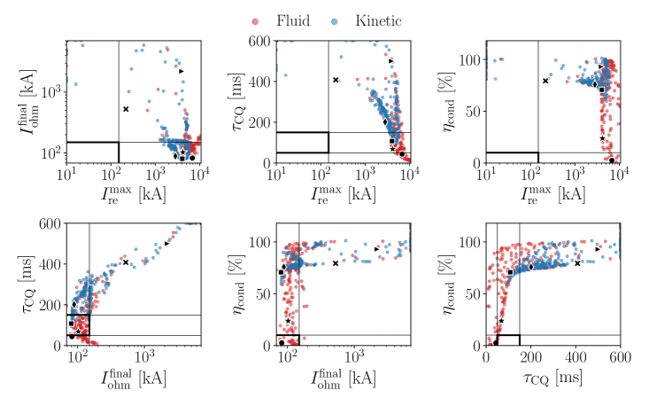
Figure 8: Projections of the simulation data set to all the two-dimensional subspaces of the figure of merit space $({I_{\rm re}^{\rm repr}},{I_{\Omega}^{\rm final}},{\tau_{\rm CQ}},{\eta_{\rm cond}})$, corresponding to the optimizations of the activated scenario. Both kinetic (blue) and fluid (red) simulations are shown. The intervals of safe operation for each cost function component is indicated by the black lines. This figure illustrates the trade-off between the different cost function components. The optimal samples found during the optimizations using the fluid (kinetic) model is indicated by a black star (diamond), while the other cases in table 1 are indicated as black markers of different shapes. Samples located outside of the plotted domains are placed at the edges.

An important similarity between our result and those in (Pusztai et al., 2023) is that we do not find any ${n_{\rm D}}$-${n_{\rm Ne}}$ combinations yielding tolerable or close to tolerable figures of merit in the activated case. For the full explored region, ${\mathcal{L}}\gg 1$, and as we mentioned earlier, the cost function was not designed to be particularly informative at these values. In order to study correlations and trade-offs between different figures of merit, another approach is needed.

We can utilize that each simulation which we have performed corresponds to a point in the four dimensional parameter space spanned by our four figures of merit, i.e. $({I_{\rm re}^{\rm repr}},{I_{\Omega}^{\rm final}},{\tau_{\rm CQ}},{\eta_{\rm cond}})$. In figure 8, these points have been projected on two-dimensional subspaces spanned by pairs of the figures of merit, which illustrates potential trade-offs between each pair. The panels in the top row clarify that for scenarios with ${I_{\rm re}^{\rm repr}}<$1\text{\,}\mathrm{M}\mathrm{A}$$, ${\tau_{\rm CQ}}>$400\text{\,}\mathrm{m}\mathrm{s}$$ and ${\eta_{\rm cond}}>$75\text{\,}\mathrm{\char 37\relax}$$. More specifically, the correlation between ${I_{\rm re}^{\rm repr}}$ and ${\eta_{\rm cond}}$ suggests that it is not possible to achieve moderate values for the runaway current and the transported heat fraction simultaneously – when ${I_{\rm re}^{\rm repr}}<$4\text{\,}\mathrm{M}\mathrm{A}$$ then ${\eta_{\rm cond}}>$75\text{\,}\mathrm{\char 37\relax}$$, and vice versa. This is related to the almost rectangular envelope bounding the point cloud from the side of low values in the ${I_{\rm re}^{\rm repr}}$–${\eta_{\rm cond}}$ panel.

Disregarding the runaway current, there are some points of safety overlap for the other three figures of merit; see the lower panels of figure 8. All simulations with ${\tau_{\rm CQ}}\in[50,150]\,$ms have ${I_{\Omega}^{\rm final}}<$150\text{\,}\mathrm{k}\mathrm{A}$$, and since there is a slight overlap between ${\tau_{\rm CQ}}\in[50,150]\,$ms and ${\eta_{\rm cond}}<$10\text{\,}\mathrm{\char 37\relax}$$, here ${I_{\Omega}^{\rm final}}<$150\text{\,}\mathrm{k}\mathrm{A}$$ as well. This can be related back to figure 6, where we see a small region of overlap for safe values of ${\tau_{\rm CQ}}$ and ${\eta_{\rm cond}}$, as well as the safe region for ${\tau_{\rm CQ}}$ being almost fully covered by the safe region for ${I_{\Omega}^{\rm final}}$.

Being able to visualize correlations between the cost function components and which regions of the ${n_{\rm D}}$-${n_{\rm Ne}}$ space corresponds to safe regions of the figures of merits are among the benefits of using a stochastic and exploratory optimization algorithm such as Bayesian optimization. This feature has enabled the exploration of how kinetic and fluid simulations compare for a large variety of scenarios, while simultaneously yielding information on the disruption evolution not just for the most optimal case but for the full region of interest in the ${n_{\rm D}}$-${n_{\rm Ne}}$ space. Such comprehensive comparison or thorough exploration of MMI of deuterium and neon would not have been possible with a more traditional optimization algorithm, such as gradient descent or the comparison of just a few scenarios.

5 Conclusions

We have compared kinetic and fluid simulations of disruptions with massive material injection for an ITER-like tokamak setup. With this objective in mind, we derived and implemented kinetic runaway electron generation sources for the Compton scattering and tritium beta decay mechanisms. Furthermore, we investigated how the hot-tail generation compares between the two models, both for activated and non-activated scenarios. Comprehensive fluid-kinetic comparisons were facilitated using Bayesian optimization of the injected densities of deuterium and neon, which enabled exploration of a large variety of different disruption scenarios.

We found that while kinetic and fluid disruption simulations representing activated scenarios generated similar results, there were major differences for the non-activated scenarios, and this was caused by differences in the fluid and kinetic hot-tail generation dynamics. Since the kinetic model evolves the distribution function of the superthermal electrons in the simulations, it takes transport of these particles due to magnetic perturbations into account, while the model distribution used to derive the hot-tail generation rate used in the fluid simulations does not. This has a high impact on the non-activated simulations since this transport leads to a depletion of the distribution function, which limits the runaway electron generation from the hot-tail mechanism in the kinetic simulations.

In the activated case, however, there is a constant generation of superthermal electrons in the kinetic simulations due to the activated sources, which acts against the depletion due to transport, and thus makes the difference between the fluid and kinetic models less severe. Furthermore, the additional generation of runaway electrons from the activated sources reduces the impact of the hot-tail generation on the magnitude of the runaway current during the CQ, and thus makes errors in the hot-tail generation rate less significant.

The cost function used for the Bayesian optimization was carefully designed, with the feature of safe disruption simulations corresponding to cost function values below unity. This had a significant impact on the cost function landscape in the explored MMI density region and the optima found during the optimization, when compared to a similar optimization done in (Pusztai et al., 2023).

Outstanding issues that remain to be investigated include the effect of vertical displacements events and other instabilites on the runaway electron dynamics. Additionally, there might be remnant magnetic perturbations even after the thermal quench, which will affect the final runaway current. Finally, the injected material will in reality not be distributed uniformly. The impact of radial inhomogeneities in the assimilated material were, to some extent, explored by Pusztai et al. (2023), finding beneficial effects of outward peaking neon and inward peaking deuterium distributions. However, such inhomogeneities might be less consequential for the runaway current evolution in the presence of an effective particle transport during the TQ (Vallhagen et al., 2024).

Funding

This work was supported by the Swedish Research Council (Dnr.  2022-02862). The work has been carried out within the framework of the EUROfusion Consortium, funded by the European Union via the Euratom Research and Training Programme (Grant Agreement No 101052200 — EUROfusion). Views and opinions expressed are however those of the authors only and do not necessarily reflect those of the European Union or the European Commission. Neither the European Union nor the European Commission can be held responsible for them.

Declaration of Interests

The authors report no conflict of interest.

Appendix A Cost function details

Here we detail two aspects of the cost function presented in section 3.2 – the representative runaway current and the impact of choice of $p$-norm.

A.1 Representative runaway current

As described in section 3.2, we considered two plausible ways to give a representative value for the runaway current; the maximum or the value at the time when ${I_{\rm re}}=0.95{I_{\rm p}}$. If a runaway current plateau is reached during the disruption, the runaway current will in most cases be slowly but monotonically increasing with time. In this case the maximum runaway current will be dependent on the simulation length, which makes the resulting value arbitrary – see figure 9.a.

Using the 95-percent runaway current would solve this problem, but it is undetermined when ${I_{\rm re}}(t)<0.95{I_{\rm p}}(t)$ throughout the simulation (figure 9.b) or when ${I_{\rm re}^{95\,\%}}$ for several $t$ (figure 9.c). Furthermore, for a hypothetical case where the runaway current near the end of the simulation fulfils ${I_{\rm re}}=0.95{I_{\rm p}}$ while being small, but peaks early during the simulation with an order $\sim$1\text{\,}\mathrm{M}\mathrm{A}$$ without reaching $95\text{\,}\mathrm{\char 37\relax}$ of the plasma current, as in figure 9.d, ${I_{\rm re}^{95\,\%}}$ would not be a representative value.

\begin{overpic}[width=341.43306pt]{figs/runaway_current.pdf} \put(22.5,25.0){(a)} \put(45.5,25.0){(b)} \put(68.6,25.0){(c)} \put(91.4,25.0){(d)} \end{overpic}

Figure 9: (a) A runaway plateau is reached during the disruption, such that the runaway current is slowly increasing and ${I_{\rm re}^{\rm max}}$ depends on the simulation length. If the simulation is stopped at $200\text{\,}\mathrm{m}\mathrm{s}$ ($150\text{\,}\mathrm{m}\mathrm{s}$) the blue (purple) star marks ${I_{\rm re}^{\rm max}}$. (b) The criteria for ${I_{\rm re}^{95\,\%}}$ is never fulfilled. (c) The criteria for ${I_{\rm re}^{95\,\%}}$ is fulfilled more than once. (d) The runaway current peaks significantly early during the simulation, but reaches $95\text{\,}\mathrm{\char 37\relax}$ of the total plasma current when both currents are negligible.

To address all of these shortcomings, we have chosen to use a combination of the maximum and 95-percent current as our representative value for the runaway current. More specifically, we will define ${I_{\rm re}^{\rm repr}}=\min_{t}\{{I_{\rm re}^{\rm max}},{I_{\rm re}^{95\,\%}}\}$.

A.2 Choice of p-norm

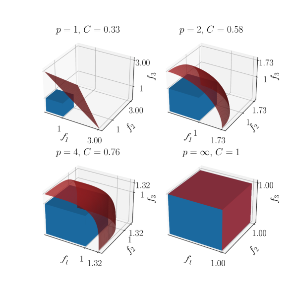
Figure 10: Illustration of the relation between $p$-norm and accuracy of ${\mathcal{L}}\leq 1$ implying safety. For this example, the cost function consists of three components $f_{1}$, $f_{2}$ and $f_{3}$. The blue box represents the safe operational region and the red surface implies the ${\mathcal{L}}=1$ surface. Note that the red surface intersects the axes at $1/C$.

In section 3.2, the cost function is described as being designed such that if all components are within their intervals of safe operation the cost function should be smaller than one. This was partly achieved by combining the cost function components using the Euclidean norm. In order for safety to be equivalent with the cost function ${\mathcal{L}}\leq 1$, we would need to use the maximum norm instead, i.e.

$${\mathcal{L}}=\max{\left(\frac{{I_{\rm re}^{\rm repr}}}{$150\text{\,}\mathrm{k}\mathrm{A}$},\frac{{I_{\Omega}^{\rm final}}}{$150\text{\,}\mathrm{k}\mathrm{A}$},\frac{{\eta_{\rm cond}}}{$10\text{\,}\mathrm{\char 37\relax}$},\frac{\absolutevalue{{\tau_{\rm CQ}}-$100\text{\,}\mathrm{m}\mathrm{s}$}}{$50\text{\,}\mathrm{m}\mathrm{s}$}\right)}.$$ (19)

However, this would result in the cost function not being once differentiable and only one component would contribute with information about the disruption scenario to the optimizer in any given point.

On the other hand, the components could be combined by simply averaging them, i.e.

$${\mathcal{L}}=\frac{1}{4}\left(\frac{{I_{\rm re}^{\rm repr}}}{$150\text{\,}\mathrm{k}\mathrm{A}$}+\frac{{I_{\Omega}^{\rm final}}}{$150\text{\,}\mathrm{k}\mathrm{A}$}+\frac{{\eta_{\rm cond}}}{$10\text{\,}\mathrm{\char 37\relax}$}+\frac{\absolutevalue{{\tau_{\rm CQ}}-$100\text{\,}\mathrm{m}\mathrm{s}$}}{$50\text{\,}\mathrm{m}\mathrm{s}$}\right).$$ (20)

While this would imply ${\mathcal{L}}\leq 1$ for all four parameters being inside of their safe operational interval, the opposite implication would not be true, namely ${\mathcal{L}}\leq 1$ implying safety. If there would be a case where only component $x$ is non-zero, this component may rise to four times its safe value with ${\mathcal{L}}\leq 1$ still satisfied.

Both (19) and (20) are extreme special cases of the $p$-norm, namely $p=\infty$ and $p=1$ respectively. The order of the $p$-norm is thus the trade-off parameter between the largest normalized component dominating the cost function value and thus losing information about the other parameters, and having unity as the exact border between safe and unsafe parameter choices. For safety to be implied by ${\mathcal{L}}\leq 1$, the weight of each component must be set as $C=1/(n)^{1/p}$ for $n$ cost function components. In figure 10, the relation between the value of $p$ and the accuracy of ${\mathcal{L}}\leq 1$ implying safety is illustrated for three arbitrary components $f_{1}$, $f_{2}$ and $f_{3}$. We deemed the Euclidean norm ($p=2$) to be close enough to ${\mathcal{L}}\leq 1$ implying safety, without any component being too dominant while large. With four components, any component can at most be a factor $1/C=2$ too large for ${\mathcal{L}}\leq 1$, and if ${\mathcal{L}}\leq 0.5$ it is definitely safe.

References

- Berger et al. (2022) Berger, E., Pusztai, I., Newton, S.L., Hoppe, M., Vallhagen, O., Fil, A. & Fülöp, T. 2022 Runaway dynamics in reactor-scale spherical tokamak disruptions. Journal of Plasma Physics 88 (6), 905880611.
- Breizman et al. (2019) Breizman, B.N., Aleynikov, P., Hollmann, E.M. & Lehnen, M. 2019 Physics of runaway electrons in tokamaks. Nuclear Fusion 59 (8), 083001.
- Connor & Hastie (1975) Connor, J.W. & Hastie, R.J. 1975 Relativistic limitations on runaway electrons. Nuclear Fusion 15 (3), 415–424.
- Fermi (1934) Fermi, E. 1934 Versuch einer Theorie der -Strahlen. I. Zeitschrift für Physik 88 (3-4), 161–177.
- Garnett (2023) Garnett, R. 2023 Bayesian Optimization. Padstow, UK: Cambridge University Press, stochastic processes: p. 8, 16–17; Matérn kernel: p. 51–52; Expected improvement acquisition function: p. 127–129.
- Helander et al. (2002) Helander, P., Eriksson, L-G. & Andersson, F. 2002 Runaway acceleration during magnetic reconnection in tokamaks. Plasma Physics and Controlled Fusion 44 (12B), B247.
- Hender et al. (2007) Hender, T.C., Wesley, J.C., Bialek, J., Bondeson, A., Boozer, A.H., Buttery, R.J., Garofalo, A., Goodman, T.P., Granetz, R.S., Gribov, Y., Gruber, O., Gryaznevich, M., Giruzzi, G., Günter, S., Hayashi, N., Helander, P., Hegna, C.C., Howell, D.F., Humphreys, D.A., Huysmans, G.T.A., Hyatt, A.W., Isayama, A., Jardin, S.C., Kawano, Y., Kellman, A., Kessel, C., Koslowski, H.R., Haye, R.J. La, Lazzaro, E., Liu, Y.Q., Lukash, V., Manickam, J., Medvedev, S., Mertens, V., Mirnov, S.V., Nakamura, Y., Navratil, G., Okabayashi, M., Ozeki, T., Paccagnella, R., Pautasso, G., Porcelli, F., Pustovitov, V.D., Riccardo, V., Sato, M., Sauter, O., Schaffer, M.J., Shimada, M., Sonato, P., Strait, E.J., Sugihara, M., Takechi, M., Turnbull, A.D., Westerhof, E., Whyte, D.G., Yoshino, R., Zohm, H. & the ITPA MHD, Disruption and Magnet Group 2007 Chapter 3: MHD stability, operational limits and disruptions. Nuclear Fusion 47 (6), S128–S202.
- Hesslow et al. (2019a) Hesslow, L., Embréus, O., Vallhagen, O. & Fülöp, T. 2019a Influence of massive material injection on avalanche runaway generation during tokamak disruptions. Nuclear Fusion 59 (8), 084004.
- Hesslow et al. (2019b) Hesslow, L., Unnerfelt, L., Vallhagen, O., Embréus, O., Hoppe, M., Papp, G. & Fülöp, T. 2019b Evaluation of the Dreicer runaway generation rate in the presence of high- impurities using a neural network. Journal of Plasma Physics 85 (6), 475850601.
- Hollmann et al. (2015) Hollmann, E.M., Aleynikov, P.B., Fülöp, T., Humphreys, D.A, Izzo, V.A., Lehnen, M., Lukash, V.E., Papp, G., Pautasso, G., Saint-Laurent, F. & Snipes, J.A. 2015 Status of research toward the ITER disruption mitigation system. Physics of Plasmas 22 (2), 021802.
- Hoppe et al. (2021a) Hoppe, M., Embréus, O. & Fülöp, T. 2021a DREAM: A fluid-kinetic framework for tokamak disruption runaway electron simulations. Computer Physics Communications 268, 108098.
- Hoppe et al. (2021b) Hoppe, M., Hesslow, L., Embréus, O., Unnerfelt, L., Papp, G., Pusztai, I., Fülöp, T., Lexell, O., Lunt, T., Macusova, E., McCarthy, P.J., Pautasso, G., Pokol, G.I., Por, G., Svensson, P., the ASDEX Upgrade team & the EUROfusion MST1 team 2021b Spatiotemporal analysis of the runaway distribution function from synchrotron images in an ASDEX Upgrade disruption. Journal of Plasma Physics 87 (1), 855870102.
- Izzo et al. (2022) Izzo, V.A., Pusztai, I., Särkimäki, K., Sundström, A., Garnier, D.T., Weisberg, D., Tinguely, R.A., Paz-Soldan, C., Granetz, R.S. & Sweeney, R. 2022 Runaway electron deconfinement in SPARC and DIII-D by a passive 3D coil. Nuclear Fusion 62 (9), 096029.
- Krane (1988) Krane, K.S. 1988 Introductory Nuclear Physics. John Wiley & Sons.
- Lehnen & the ITER DMS task force (2021) Lehnen, M. & the ITER DMS task force 2021 The ITER disruption mitigation system - design progress and design validation. Presented at Theory and Simulation of Disruptions Workshop, PPPL.
- Martín-Solís et al. (2017) Martín-Solís, J.R., Loarte, A. & Lehnen, M. 2017 Formation and termination of runaway beams in ITER disruptions. Nuclear Fusion 57 (6), 066025.
- Miller et al. (1998) Miller, R.L., Chu, M.S., Greene, J.M., Lin-Liu, Y.R. & Waltz, R.E. 1998 Noncircular, finite aspect ratio, local equilibrium model. Physics of Plasmas 5 (4), 973–978.
- Nogueira (2014) Nogueira, F. 2014 Bayesian optimization: Open source constrained global optimization tool for Python.
- Pusztai et al. (2023) Pusztai, I., Ekmark, I., Bergström, H., Halldestam, P., Jansson, P., Hoppe, M., Vallhagen, O. & Fülöp, T. 2023 Bayesian optimization of massive material injection for disruption mitigation in tokamaks. Journal of Plasma Physics 89 (2), 905890204.
- Rechester & Rosenbluth (1978) Rechester, A.B. & Rosenbluth, M.N. 1978 Electron heat transport in a tokamak with destroyed magnetic surfaces. Phys. Rev. Lett. 40, 38–41.
- Redl et al. (2021) Redl, A., Angioni, C., Belli, E. & Sauter, O. 2021 A new set of analytical formulae for the computation of the bootstrap current and the neoclassical conductivity in tokamaks. Physics of Plasmas 28 (2), 022502.
- Rosenbluth & Putvinski (1997) Rosenbluth, M.N. & Putvinski, S.V. 1997 Theory for avalanche of runaway electrons in tokamaks. Nuclear Fusion 37 (10), 1355.
- Smith & Verwichte (2008) Smith, H.M. & Verwichte, E. 2008 Hot tail runaway electron generation in tokamak disruptions. Physics of Plasmas 15 (7), 072502.
- Svenningsson (2020) Svenningsson, I. 2020 Hot-tail runaway electron generation in cooling fusion plasmas. Master’s thesis, Chalmers University of Technology, https://hdl.handle.net/20.500.12380/300899.
- Svenningsson et al. (2021) Svenningsson, I., Embréus, O., Hoppe, M., Newton, S.L. & Fülöp, T. 2021 Hot-tail runaway seed landscape during the thermal quench in tokamaks. Phys. Rev. Lett. 127 (3), 035001.
- Tinguely et al. (2021) Tinguely, R.A., Izzo, V.A., Garnier, D.T., Sundström, A., Särkimäki, K., Embréus, O., Fülöp, T., Granetz, R.S., Hoppe, M., Pusztai, I. & Sweeney, R. 2021 Modeling the complete prevention of disruption-generated runaway electron beam formation with a passive 3D coil in SPARC. Nuclear Fusion 61 (12), 124003.
- Tinguely et al. (2023) Tinguely, R.A., Pusztai, I., Izzo, V.A., Särkimäki, K., Fülöp, T., Garnier, D.T., Granetz, R.S., Hoppe, M., Paz-Soldan, C., Sundström, A. & Sweeney, R. 2023 On the minimum transport required to passively suppress runaway electrons in SPARC disruptions. Plasma Physics and Controlled Fusion 65 (3), 034002.
- Vallhagen et al. (2020) Vallhagen, O., Embréus, O., Pusztai, I., Hesslow, L. & Fülöp, T. 2020 Runaway dynamics in the DT phase of ITER operations in the presence of massive material injection. Journal of Plasma Physics 86 (4), 475860401.
- Vallhagen et al. (2024) Vallhagen, O., Hanebring, L., Artola, F.J., Lehnen, M., Nardon, E., Fülöp, T., Hoppe, M., Newton, S.L. & Pusztai, I. 2024 Runaway electron dynamics in ITER disruptions with shattered pellet injections. submitted to Nuclear Fusion, ArXiv 2401.14167 .
- Vallhagen et al. (2022) Vallhagen, O., Pusztai, I., Hoppe, M., Newton, S.L. & Fülöp, T. 2022 Effect of two-stage shattered pellet injection on tokamak disruptions. Nuclear Fusion 62 (11), 112004.