Dirichlet Flow Matching with Applications to DNA Sequence Design

Abstract

Discrete diffusion or flow models could enable faster and more controllable sequence generation than autoregressive models. We show that naïve linear flow matching on the simplex is insufficient toward this goal since it suffers from discontinuities in the training target and further pathologies. To overcome this, we develop Dirichlet flow matching on the simplex based on mixtures of Dirichlet distributions as probability paths. In this framework, we derive a connection between the mixtures’ scores and the flow’s vector field that allows for classifier and classifier-free guidance. Further, we provide distilled Dirichlet flow matching, which enables one-step sequence generation with minimal performance hits, resulting in $O(L)$ speedups compared to autoregressive models. On complex DNA sequence generation tasks, we demonstrate superior performance compared to all baselines in distributional metrics and in achieving desired design targets for generated sequences. Finally, we show that our classifier-free guidance approach improves unconditional generation and is effective for generating DNA that satisfies design targets. Code is available at https://github.com/HannesStark/dirichlet-flow-matching.

1 Introduction

Flow matching (FM) is a generative modeling framework that provides a simulation-free means of training continuous normalizing flows (CNFs) between noise and data distributions (Lipman et al., 2022; Liu et al., 2022; Albergo & Vanden-Eijnden, 2022). Such flow models can be viewed as generalizing diffusion models (Song et al., 2021) to permit more flexible design of iterative noising processes, which have proven useful in generative modeling on non-euclidean spaces such as compact Riemannian manifolds (Chen & Lipman, 2023; Bose et al., 2023). However, existing formulations of flow matching have focused on continuous spaces and have yet to treat discrete categorical data—a notable shortcoming considering the many important applications of discrete generative modeling such as text generation and biological sequence design (Avdeyev et al., 2023).

In this work, we introduce Dirichlet flow matching for generative modeling of discrete categorical data and sequences over such data. We frame such modeling as a transport problem between a uniform density over the probability simplex and a finitely supported distribution over the vertices of the simplex. We then learn a continuous vector field to parameterize this transport based on a conditional noising process that generates a time-evolving Dirichlet distribution. Naïvely, it may appear more straightforward to define a noising process that linearly interpolates between data and noise, as is the dominant approach in flow matching on $\mathbb{R}^{n}$ (Liu et al., 2022; Lipman et al., 2022; Pooladian et al., 2023) and which can be trivially adapted to the simplex. However, we show that such an approach—which we call linear flow matching—suffers from pathological behavior due to the contracting support of the resulting conditional probability paths. We carefully engineer Dirichlet FM to avoid these shortcomings while retaining the advantages of flow matching by being significantly simpler—both computationally and conceptually—than DDSM (Avdeyev et al., 2023), a discrete diffusion model that also relaxes data onto the simplex. Thanks to these properties, we posit (and confirm) that Dirichlet FM is significantly more fit for modeling complex discrete distributions than either linear FM or DDSM.

 

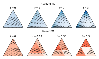
Figure 1: Overview of Dirichlet flow matching. Left: starting from uniform noise on the probability simplex, we define conditional probability paths that approach a point mass at the vertex via a one-parameter family of Dirichlet distributions. We view a sequence of tokens as a sequence of simplices for which the probability path corresponds to noising tokens via superposition with all other possible tokens (during inference, the simplices depend on each other through a joint denoiser). Right: Comparison of the marginal probability paths and vector fields of Dirichlet and linear FM. The vector fields of Dirichlet FM are smooth in time and space, unlike linear FM.

Dirichlet FM is equipped with several features that showcase its potential as a generative modeling framework. A key aspect of modern frameworks such as diffusion is the ability to implement guidance towards a target class or attribute (Dhariwal & Nichol, 2021; Ho & Salimans, 2022). While flow matching guidance has been explored for (diffusion-like) Gaussian noising processes in $\mathbb{R}^{n}$ (Dao et al., 2023; Zheng et al., 2023), no general theory of flow matching guidance is available. However, by deriving a relationship between the score of a mixture of Dirichlets and the resulting flow, we implement both classifier guidance and classifier-free guidance within the framework of Dirichlet FM. Additionally, unlike autoregressive models or diffusion models that inject categorical noise (Austin et al., 2021; Hoogeboom et al., 2021; Campbell et al., 2022), the sampling process of Dirichlet FM defines a deterministic map between noise and data. Hence, we can distill the sampling process and generate arbitrarily long sequences in a single forward pass.

We evaluate Dirichlet FM on three DNA sequence datasets with several complex tasks that pose diverse challenges. First, we demonstrate that Dirichlet FM better generates promoter DNA sequences with desired regulatory activity compared to baselines such as an autoregressive language model or discrete diffusion models, including DDSM (Avdeyev et al., 2023). Second, we show on two enhancer DNA sequence datasets that Dirichlet FM improves upon autoregressive language modeling in capturing the data distribution with an FBD (distributional similarity) of 1.9 vs. 36.0 in Melanoma DNA and 1.0 vs. 25.2 in Fly Brain DNA. Third, we demonstrate that Dirichlet FM guidance can improve unconditional sequence generation and generate cell-type specific enhancer DNA sequences that improve upon the (experimentally validated) sequences of Taskiran et al. (2023). Lastly, distilled Dirichlet FM generates sequences in a single step, resulting in orders-of-magnitude speedups with minimal performance degradation.

2 Background

2.1 Flow Matching

In flow matching (Lipman et al., 2022; Liu et al., 2022; Albergo & Vanden-Eijnden, 2022), we consider a noisy distribution $\mathbf{x}_{0}\sim q_{0}$ and data distribution $\mathbf{x}_{1}\sim p_{\text{data}}$ and regress a neural network against a vector field that transports $q(\mathbf{x}_{0})$ to $p_{\text{data}}(\mathbf{x}_{1})$. To do so, we define a conditional probability path—a time-evolving distribution $p_{t}(\mathbf{x}\mid\mathbf{x}_{1}),t\in[0,1]$ conditioned on $\mathbf{x}_{1}$ with boundary conditions $p_{0}(\mathbf{x}\mid\mathbf{x}_{1})=q(\mathbf{x})$ and $p_{1}(\mathbf{x}\mid\mathbf{x}_{1})\approx\delta(\mathbf{x}-\mathbf{x}_{1})$. We additionally assume knowledge of a conditional vector field $u_{t}(\mathbf{x}~{}\mid~{}\mathbf{x}_{1})$ that generates $p_{t}(\mathbf{x}\mid\mathbf{x}_{1})$, i.e. satisfying the transport equation

$$\frac{\partial}{\partial t}p_{t}+\nabla\cdot(p_{t}u_{t})=0$$ (1)

Then, the marginal probability path

$$p_{t}(\mathbf{x})=\int p_{t}(\mathbf{x}\mid\mathbf{x}_{1})p_{\text{data}}(\mathbf{x}_{1})\,d\mathbf{x}_{1}$$ (2)

interpolates between noise $p_{0}=q_{0}$ and data $p_{1}\approx p_{\text{data}}$ and is generated by the marginal vector field

$$v_{t}(\mathbf{x})=\int u_{t}(\mathbf{x}\mid\mathbf{x}_{1})\frac{p_{t}(\mathbf{x}\mid\mathbf{x}_{1})p_{\text{data}}(\mathbf{x}_{1})}{p_{t}(\mathbf{x})}\,d\mathbf{x}_{1}$$ (3)

Thus, by learning and integrating a neural network $\hat{v}(\mathbf{x},t;\theta)\approx v_{t}(\mathbf{x})$, we can generate data from noisy samples $\mathbf{x}_{0}\sim q$. The core design decision is the choice of appropriate conditional probability path $p_{t}(\mathbf{x}\mid\mathbf{x}_{1})$ and associated vector field $u_{t}(\mathbf{x}\mid\mathbf{x}_{1})$. Although it is possible to define these directly, it is often simpler to instead define a conditional flow map $\psi_{t}(\mathbf{x}_{0}\mid\mathbf{x}_{1})$ that directly transports $\mathbf{x}_{0}\sim q$ to the intermediate distribution $p_{t}(\mathbf{x}\mid\mathbf{x}_{1})$. The flow map immediately provides the corresponding vector field:

$$u_{t}(\mathbf{x}\mid\mathbf{x}_{1})=\frac{d}{dt}\psi_{t}(\mathbf{x}_{0}\mid\mathbf{x}_{1})$$ (4)

With this formulation, the required boundary conditions simplify to $\psi_{0}(\mathbf{x}_{0}\mid\mathbf{x}_{1})=\mathbf{x}$ and $\psi_{1}(\mathbf{x}_{0}\mid\mathbf{x}_{1})=\mathbf{x}_{1}$. As advocated by several works (Liu et al., 2022; Lipman et al., 2022; Pooladian et al., 2023; Tong et al., 2023), the flow map (also called interpolant) is often chosen to follow the simplest possible path between the two endpoints—e.g., linear in Euclidean spaces and geodesic on Riemannian manifolds (Chen & Lipman, 2023).

2.2 Related Discrete Diffusion Model Works

Existing discrete diffusion frameworks can be split into 4 categories. Firstly, simplex-based approaches frame discrete data as vertices of a simplex and generate it starting from a Dirichlet prior over the whole simplex (Richemond et al., 2022; Floto et al., 2023). Among those, DDSM (Avdeyev et al., 2023) is most related to our work and converges to a Dirichlet distribution via Jacobi diffusion processes and the stick-breaking transform. We note that none of these simplex-based approaches feature Dirichlet distributions as intermediate distributions of the noising process—a key aspect of our approach.

The second class of discrete diffusion models fully relaxes discrete data into continuous space without any constraints and uses, e.g., a standard Gaussian as prior (Han et al., 2022; Chen et al., 2023; Frey et al., 2024). The third paradigm, established by D3PM (Austin et al., 2021), operates on discrete samples of noise distributions constructed by injecting discrete noise into data (Campbell et al., 2022; Igashov et al., 2024; Vignac et al., 2023; Penzar et al., 2023). Lastly, latent discrete diffusion models train an additional network to obtain continuous latents for which they train a conventional diffusion model (Dieleman et al., 2022; Li et al., 2023).

2.3 Promoter and Enhancer DNA

DNA is a sequence with base pairs as tokens (3 billion for humans) and a vocabulary of 4 nucleotides (A, T, C, G). Parts of DNA encode genes that are transcribed into mRNA and then translated to functional proteins. Promoters and enhancers refer to noncoding portions of DNA that regulate the expression level of these genes and play important roles in eukaryotic organisms such as humans (Dunham et al., 2012; Luo et al., 2020). More specifically, a promoter for a gene is the DNA sequence next to the gene where the transcriptional machinery binds and starts transcribing DNA to mRNA (Haberle & Stark, 2018). Meanwhile, enhancers are sequences that can be distant in the DNA sequence (millions of base pairs) but are close in 3D space (Panigrahi & O’Malley, 2021) and regulate the recruitment of this transcriptional machinery. Unlike promoters, enhancers often regulate transcription in specific cell types. Hence, while both types of DNA subsequences are important for gene therapy (Whalen, 1994), the cell type specificity of enhancers enables targeting, e.g., only cancer cells.

Designing enhancers. Recently Taskiran et al. (2023) and de Almeida et al. (2023) demonstrated cell type-specific enhancer design via an optimization procedure starting from an initial sequence guided by a cell-type activity classifier. However, such sequence designs may not follow the empirical distribution of enhancers, which would be captured by a generative model. Our work sets the foundation for more principled conditional sequence design by learning and drawing from conditional data distributions.

3 Method

3.1 Flow Matching on the Simplex

Let $S_{K}$ be the probability simplex in $K$-dimensional space:

$$S_{K}=\{\mathbf{x}=(x_{1},\ldots x_{K})^{T}\in\mathbb{R}^{K}\mid\boldsymbol{1}^{T}\mathbf{x}=1,\mathbf{x}\geq 0\}$$ (5)

Given a $K$-class categorical distribution with probabilities $p_{i},\sum_{i=1}^{K}p_{i}=1$, we relax this distribution into continuous space by converting it to a mixture of point masses at the vertices of $S_{k}$ (with $\mathbf{e}_{i}$ as the $i$th one-hot vector):

$$p_{\text{data}}(\mathbf{x})=\sum_{i=1}^{K}p_{i}\delta(\mathbf{x}-\mathbf{e}_{i})$$ (6)

We then define the noisy prior to be the uniform density on the simplex, or a Dirichlet distribution with parameter vector $\boldsymbol{\alpha}$ given by the all ones vector:

$$q_{0}(\mathbf{x})=\operatorname{Dir}(\mathbf{x};\boldsymbol{\alpha}=(1,\ldots 1)^{T})=\Gamma(K)$$ (7)

Our objective is then to learn a vector field, using some choice of conditional probability path (discussed later), to transport $q_{0}$ to $p_{\text{data}}$. Typically, the neural network directly parameterizes the vector field and is trained via the $L_{2}$-like conditional flow-matching loss

$$\mathcal{L}(\theta)=\mathbb{E}[\lVert u_{t}(\mathbf{x}\mid\mathbf{x}_{1})-\hat{v}(\mathbf{x},t;\theta)\rVert^{2}]$$ (8)

where the expectation is taken over $t\sim\mathcal{U}[0,1],\mathbf{x}_{1}\sim p_{\text{data}},\mathbf{x}\sim p_{t}(\cdot\mid\mathbf{x}_{1})$. However, we instead train a denoising classifier via a cross-entropy loss

$$\mathcal{L}(\theta)=\mathbb{E}[\log\hat{p}(\mathbf{x}_{1}\mid\mathbf{x};\theta)]$$ (9)

At inference time, we then parameterize the vector field via

$$\hat{v}(\mathbf{x},t;\theta)=\sum_{i=1}^{K}u_{t}(\mathbf{x}\mid\mathbf{x}_{1}=\mathbf{e}_{i})\hat{p}(\mathbf{x}_{1}=\mathbf{e}_{i}\mid\mathbf{x};\theta)$$ (10)

It can be shown (Appendix A) that the two losses have the same minimizer, and thus, the cross-entropy is a valid flow-matching objective. The advantages of this approach are twofold: (1) it ensures that the learned vector field is restricted to the tangent plane of the simplex (i.e., the components sum to zero), and (2) the conditional vector field does not need to be evaluated at training time.

For simplicity, our discussion focuses on modeling categorical data on the simplex. However, in practice, we are interested in sequences of variables relaxed onto the multi-simplex $S_{K}^{N}$. At inference time, the simplices depend on each other through a learned denoiser that outputs token-wise logits conditioned on all noisy inputs.

3.2 Designing Simplex Flow Matching

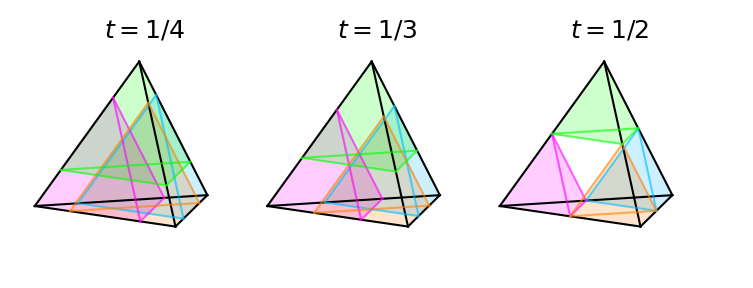
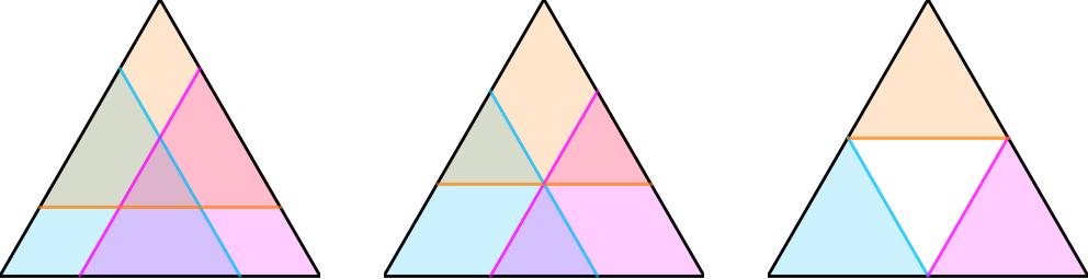
Figure 2: Pathological behavior of linear flow matching on the simplex with $K=4$ (top) and $K=3$ (bottom). Each color represents a conditional probability path evolving over time toward its target vertex. At $t=1/4$, $t=1/3$, and $t=1/2$, the region of overlap between 4, 3, and 2 conditional probability paths disappears, respectively, corresponding to a shrinking set of possible values of $\mathbf{x}_{1}\mid\mathbf{x}$ for any $\mathbf{x}$.

As outlined in Section 2.1, there are two options to define a conditional probability path $p_{t}(\mathbf{x}\mid\mathbf{x}_{1})$ and corresponding vector field $u_{t}(\mathbf{x}\mid\mathbf{x}_{1})$ to train a flow model with:

1. Interpolant perspective: Define an interpolant $\psi_{t}(\mathbf{x}_{0}\mid\mathbf{x}_{1})$, which provides the density $p_{t}(\mathbf{x}\mid\mathbf{x}_{1})$ implicitly but allows one to easily sample from it, and obtain the conditional vector field trivially by taking the derivative $u_{t}=\partial_{t}\psi_{t}$.

2. Probability path perspective: Define $p_{t}(\mathbf{x}\mid\mathbf{x}_{1})$ explicitly and solve for $u_{t}(\mathbf{x}\mid\mathbf{x}_{1})$ that satisfies the transport equation which can be non-trivial.

Following extant works on flow matching, the most natural way to proceed for the simplex would be to follow the interpolant perspective and use the linear flow map employed in Lipman et al. (2022); Pooladian et al. (2023):

$$\psi_{t}(\mathbf{x}_{0}\mid\mathbf{x}_{1}) =(1-t)\mathbf{x}_{0}+t\mathbf{x}_{1}$$ (11)

$$u_{t}(\mathbf{x}\mid\mathbf{x}_{1}) =\frac{\mathbf{x}_{1}-\mathbf{x}}{1-t}=\mathbf{x}_{1}-\mathbf{x}_{0}$$ (12)

Since $S_{K}$ is a Euclidean space, these operations remain well-defined, and the interpolant transports all points on the simplex to $\mathbf{x}_{1}$ at $t=1$ via straight paths. However, a pathological property emerges when such conditional probability paths are marginalized over $p_{\text{data}}(\mathbf{x}_{1})$ over the course of flow matching training:

Proposition 1.

Suppose that a flow matching model is trained with the linear flow map (Equation 11). Then, for all $k=2,\ldots K$ and $\mathbf{x}\sim p_{t}(\mathbf{x})$, the converged model posterior $p(\mathbf{x}_{1}\mid\mathbf{x})\propto p_{t}(\mathbf{x}\mid\mathbf{x}_{1})p_{\text{data}}(\mathbf{x}_{1})$ has support over at most $k-1$ vertices for times $t>1/k$.

Conceptually, this means that as the model transports samples on the simplex at $t=0$ to the vertices of the simplex at $t=1$, it must eliminate or rule out a possible destination vertex at each of the times $\frac{1}{K},\frac{1}{K-1},\ldots\frac{1}{2}$, if not earlier. As $K$ becomes large, an increasingly large fraction of the model capacity must be allocated to a smaller and smaller fraction of the total time and trajectory length—indeed, for all $K$, the posterior for times $t>1/2$ reduces to the $\arg\max$ operator. Further, since the marginal field is increasingly discontinuous (i.e., rapidly changing directions and settings entries to zero corresponding to eliminated vertices), the model becomes increasingly sensitive to integration step size. We posit—and empirically verify in Section 4—that these factors significantly hurt the performance of linear flow matching, especially for higher dimensionalities $K$.

Upon examination of the marginal probability paths (Figure 2), it becomes clear that this pathological behavior is due to the shrinking support of the conditional paths that arise from linear FM. Unfortunately, by following the interpolant perspective, we are unable to directly control the conditional path. Hence, to obtain a method that does not suffer from linear FM’s pathologies, we proceed with the probability path perspective and directly define the conditional probability path so that it has support on the entire simplex at all times, as described next.

3.3 Dirichlet Flow Matching

Probability path $p_{t}(\mathbf{x}\mid\mathbf{x}_{1})$.

Recall the Dirichlet distribution’s probability density function:

$$\operatorname{Dir}(\mathbf{x};\alpha_{1},\ldots\alpha_{K})=\frac{1}{\mathcal{B}(\alpha_{1},\ldots\alpha_{K})}\prod_{i=1}^{K}x_{i}^{\alpha_{i}-1}$$ (13)

Following the probability path perspective, we first define a conditional probability path with $t\in[0,\infty)$ as:

$$p_{t}(\mathbf{x}\mid\mathbf{x}_{1}=\mathbf{e}_{i})=\operatorname{Dir}(\mathbf{x};\boldsymbol{\alpha}=\boldsymbol{1}+t\cdot\mathbf{e}_{i})$$ (14)

When $t=0$, this is equal to the uniform noise distribution (Equation 7). As $t\rightarrow\infty$, the $i$th entry of the $\boldsymbol{\alpha}$ parameter vector increases while the others remain constant, concentrating the density towards a point mass on the $i$th vertex, corresponding to the $t=1$ boundary condition in standard flow matching. Hence, this family of Dirichlet distributions provides a conditional probability path with the required boundary conditions while retaining support over the entire simplex, as desired.

Vector field $u_{t}(\mathbf{x}\mid\mathbf{x}_{1})$.

Since we have chosen a conditional probability path directly rather than implicitly via an interpolant, it is more difficult to obtain the corresponding conditional vector field $u_{t}(\mathbf{x}\mid\mathbf{x}_{1})$. Indeed, there is an infinite number of such fields that generate the desired evolution of $p_{t}$. Motivated by the basic form of the linear FM, we generalize it via the following ansatz:

$$u_{t}(\mathbf{x}\mid\mathbf{x}_{1}=\mathbf{e}_{i})=C(x_{i},t)(\mathbf{e}_{i}-\mathbf{x})$$ (15)

That is, the flow still points directly towards the target vertex $\mathbf{e}_{i}$, but is rescaled by a $x_{i}$-dependent factor. The conditional vector field of linear FM satisfies this form with $C(x_{i},t)=1/(1-t)$ dependent only on $t$; we introduce the additional $x_{i}$-dependence to control the contraction of probability mass towards $\mathbf{e}_{i}$. In Appendix A.1, we derive the $C(x_{i},t)$, which gives rise to Dirichlet probability paths to be:

$$C(x_{i},t)=-\tilde{I}_{x_{i}}(t+1,K-1)\frac{\mathcal{B}(t+1,K-1)}{(1-x_{i})^{K-1}x_{i}^{t}}$$ (16)

where

$$\tilde{I}_{x}(a,b)=\frac{\partial}{\partial a}I_{x}(a,b)$$ (17)

is a derivative of the regularized incomplete beta function $I_{x}(a,b)$. Figure 3 compares the magnitude of the resulting vector field with that of linear FM as a function of distance from the target vertex. As anticipated, the field vanishes both at the target vertex and on the $(K-2)$-dimensional face directly opposite it instead of monotonically scaling with distance from the target vertex as in linear FM. This second condition means the probability density is never fully drawn away from the face and resolves the pathological behavior of linear FM. The resulting probability paths and vector fields are visualized on the simplex in Figure 1; they are continuous and smooth, unlike in linear FM.

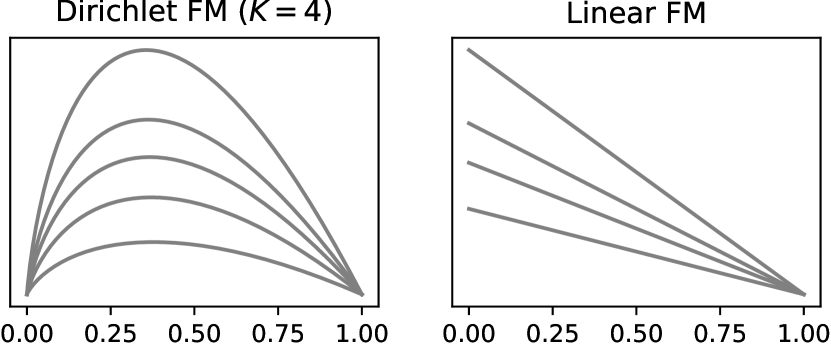
Figure 3: Vector field magnitudes of the conditional flow field $u_{t}(\mathbf{x}\mid\mathbf{x}_{1}=\mathbf{e}_{i})$ as a function of $x_{i}$ (the $i$th element of $\mathbf{x}$) plotted for varying values of $t$. In Dirichlet FM, the field vanishes at both $x_{i}=1$ (i.e., the target vertex) and $x_{i}=0$ (the opposite face).

3.4 Guidance

A key attribute of iterative generative models is the ability to continuously and gradually bias the generative process towards a class label with user-specified strength, a technique known as guidance (Dhariwal & Nichol, 2021; Ho & Salimans, 2022). Initially proposed in the context of diffusion models, where the generative process follows the score $\hat{s}(\mathbf{x},t;\theta)\approx\nabla_{\mathbf{x}}\log p_{t}(\mathbf{x})$ of the noisy data distribution, guidance is implemented by taking a linear combination of the unconditional and conditional score models

$$\hat{s}_{\text{CFG}}(\mathbf{x},t,y;\theta)=\gamma\hat{s}(\mathbf{x},t,y;\theta)+(1-\gamma)\hat{s}(\mathbf{x},t,\varnothing;\theta)$$ (18)

with $\gamma>0$ and running the generative process with this adjusted score. In the context of flow matching, Dao et al. (2023); Zheng et al. (2023) derived a relationship between the score and marginal flow for certain Gaussian probability paths and implemented flow guidance by propagating the effects of standard score adjustments to the resulting flow fields. We implement guidance for Dirichlet FM by deriving a similar relationship between the score and flow field, detailed below. Note that when $\gamma=1$, this adjustment precisely mimics the flow that would result from training only on points with class label $y$; however, similar to prior works, we find $\gamma>1$ futher enhances the guidance efficacy.

Relationship between flow and score. For the Dirichlet marginal probability path, the score can be obtained from the model posterior via the denoising score-matching identity (Song & Ermon, 2019):

$$\hat{s}(\mathbf{x},t;\theta)=\sum_{i=1}^{K}s_{t}(\mathbf{x}\mid\mathbf{x}_{1}=\mathbf{e}_{i})\hat{p}(\mathbf{x}_{1}=\mathbf{e}_{i}\mid\mathbf{x};\theta)$$ (19)

We can differentiate Equation 14 to obtain a matrix equation

$$\hat{s}=\mathbf{D}\hat{p},\quad\text{where}\quad\mathbf{D}_{ij}=\delta_{ij}\frac{t}{x_{i}}$$ (20)

Here, $\mathbf{D}$ is a $K\times K$ diagonal matrix dependent on $\mathbf{x},t$ and $\hat{s},\hat{p}\in\mathbb{R}^{n}$. (Technically, $\hat{s}$ contains both on-simplex and off-simplex components, the latter of which is ignored.) Meanwhile, the computation of the marginal flow (Equation 10) can also be written as a very similar matrix equation $\hat{v}=\mathbf{U}\hat{p}$ where the entries of $\mathbf{U}$ are given by Equation 15. Combining these, we obtain

$$\hat{v}=\mathbf{U}\mathbf{D}^{-1}\hat{s}$$ (21)

where $\mathbf{D}$ is invertible since it is diagonal with nonnegative entries. Thus, a linear relationship exists between the marginal flow and the score arising from the same model posterior.

Classifier-free guidance. Suppose we have class-conditional and unconditional flow models $\hat{v}(\mathbf{x},t,y;\theta)$ and $\hat{v}(\mathbf{x},t,\varnothing;\theta)$. Since a linear combination of scores results in a linear combination of flows, we similarly implement guidance by integrating

$$\hat{v}_{\text{CFG}}(\mathbf{x},t,y;\theta)=\gamma\hat{v}(\mathbf{x},t,y;\theta)+(1-\gamma)\hat{v}(\mathbf{x},t,\varnothing;\theta)$$ (22)

Classifier guidance. In cases where a conditional flow model is unavailable, we use the gradient of a noisy classifier to obtain a conditional score from an unconditional score:

$$\hat{s}(\mathbf{x},t,y;\theta)=\hat{s}(\mathbf{x},t,\varnothing;\theta)+\nabla_{\mathbf{x}}\log\hat{p}(y\mid\mathbf{x},t;\theta)$$ (23)

The conditional scores can then be converted into a model posterior $\hat{p}$ and then a marginal flow $\hat{v}$ via Equation 21. However, a direct application is not possible because the classifier gradients do not have the appropriate off-simplex components to ensure a valid model posterior (i.e., $\hat{p}\in S_{K}$) when operated on by $\mathbf{D}^{-1}$. Instead, we modify Equation 21 via

$$\tilde{\mathbf{D}}=\left(I-\frac{1}{K}\boldsymbol{1}\boldsymbol{1}^{T}\right)\mathbf{D}$$ (24)

corresponding to projecting the score onto the tangent plane of the simplex (i.e., $\boldsymbol{1}^{T}\hat{s}=0$). As now $\mathbf{D}$ is no longer invertible, we obtain the conditional model posterior from the score by solving $\hat{s}=\tilde{\mathbf{D}}\hat{p}$ with the additional constraint $\boldsymbol{1}^{T}\hat{p}=1$ and—since the classifier in practice may result in negative probabilities—project to the simplex via the algorithm of Wang & Carreira-Perpinán (2013).

3.5 Distillation

The aim of distillation (Salimans & Ho, 2022; Song et al., 2023; Yin et al., 2023) is to reduce the inference time of the iterative generative process by reducing the number of steps while retaining sample quality. However, for discrete diffusion models (see Section 2.2) or autoregressive language models, no distillation techniques exist, and it is unclear how to distill generative models based on discrete noise. For Dirichlet FM, inference is a deterministic ODE integration defining a map between the prior and target distribution. Hence, we can distill the teacher model (using 100 steps in our experiments) into a student model representing the map. For this, we sample the teacher to obtain pairs of noise and training targets. We use these to train the student model to reproduce the teacher distribution in a single step. With this, we are able to reduce inference times and provide the first demonstration of distillation for flow matching and for iterative generative models of discrete data.

4 Experiments

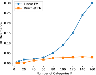
Figure 4: Scaling to higher simplex dimensions. We train on simple categorical distributions with an increasing number of categories $K$ and measure the KL divergence between the generated distributions (512k samples) and the training target distribution. Dirichlet FM scales to larger $K$ much better than linear FM.

4.1 Simplex dimension toy experiment

We first evaluate Dirichlet FM and linear FM in a simple toy experiment where the KL divergence of the generated distribution to the target distribution can be evaluated under increasing simplex dimensions. For this, we train both methods to reproduce a categorical distribution $q(\mathbf{x})=\operatorname{Cat}(K,\mathbf{a})$ where the class probabilities $\mathbf{a}$ are sampled from a uniform Dirichlet $\mathbf{a}\sim\operatorname{Dir}(\mathbf{a};\boldsymbol{1})$. To evaluate, we use the KL-divergence KL$(\tilde{p}\parallel q)$ where $\tilde{p}$ is the empirical distribution of $512,000$ model samples.

Figure 4 shows these KL-divergences for increasing sizes $K$ of the categorical distribution. Dirichlet FM is able to overfit on the simple distribution regardless of $K$. Meanwhile, Linear FM is unable to overfit on simple categorical distributions as $K$ increases, illustrating the practical implications of the pathological probability paths and discontinuous vector fields as discussed in Section 3.2.

4.2 Promoter DNA sequence design

We next assess the ability of Dirichlet FM to design DNA promoter sequences conditioned on a desired promoter profile. The experimental setup and evaluation closely follow that of DDSM (Avdeyev et al., 2023).

Data. We use a dataset of $100,000$ promoter sequences with $1,024$ base pairs extracted from a database of human promoters (Hon et al., 2017). Each sequence has a CAGE signal (Shiraki et al., 2003) annotation available from the FANTOM5 promoter atlas (Forrest et al., 2014), which indicates the likelihood of transcription initiation at each base pair ($\mathbf{r}\in\mathbb{R}^{1024}$). Sequences from chromosomes 8 and 9 are used as a test set, and the rest for training.

Table 1: Evaluation of transcription profile conditioned promoter DNA sequence design. Conditioned on a transcription profile, each method is tasked to generate a DNA sequence with that profile. The MSE is between the predicted regulatory activity of the designed sequence and the ground truth sequence. NFE refers to the number of function evaluations required for sampling. Numbers with * are from Avdeyev et al. (2023).

Method	MSE	NFE
Bit Diffusion (bit-encoding)*	.0414	100
Bit Diffusion (one-hot encoding)*	.0395	100
D3PM-uniform*	.0375	100
DDSM*	.0334	100
Language Model	.0333	1024
Linear FM	.0281	100
Dirichlet FM	.0269	100
Dirichlet FM distilled	.0278	1

Task. We train Dirichlet FM conditioned on a profile by providing it as additional input to the vector field. Following Avdeyev et al. (2023), we evaluate generated sequences with the mean squared error (MSE) between their predicted regulatory activity and that of the original sequence corresponding to the input profile. The regulatory activity is determined by the promoter-related predictions of Sei (Chen et al., 2022), a model trained on various regulatory signals.

Baselines. We compare Dirichlet FM with linear FM, discrete diffusion methods, and a language model that autoregressively generates the base pairs. The discrete diffusion baseline most related to our work is the simplex-based DDSM (Avdeyev et al., 2023). Our two other diffusion baselines are Bit Diffusion (Chen et al., 2023) and D3PM (Austin et al., 2021). All methods use the same DNA modeling architecture and training protocol that was designed and tuned by (Avdeyev et al., 2023) for DDSM. See Appendix B.1 for implementation details.

Results. Dirichlet FM is the only method that is able to outperform the language model baseline (Table 1). Linear FM performs the worst, empirically confirming the drawbacks of its discontinuous vector field and pathological probability paths. The second best method in this comparison is the distilled version of Dirichlet FM, which retains almost the same performance. This means that our distilled Dirichlet FM outperforms all other methods in a single step, which is a $100\times$ speedup compared to the diffusion models and a $1,024\times$ speedup compared to the language model in terms of number of function evaluations (NFE).

4.3 Enhancer DNA design

We now assess the performance of Dirichlet FM on DNA enhancer sequences and design evaluations that quantify both unconditional and conditional sample quality. Implementation and architecture details are in Appendix B.1.

Data. We evaluate on two enhancer sequence datasets from fly brain cells (Janssens et al., 2022) and from human melanoma cells (Atak et al., 2021). These contain 104k fly brain and 89k melanoma sequences of length 500 with cell class labels determined from ATAC-seq data (Buenrostro et al., 2013). Overall, there are 81 such classes of cells in the fly brain data and 47 in melanoma data (see Appendix B.2 for more data details).

Table 2: Evaluation of unconditional enhancer generation. Each method generates 10k sequences, and we compare their empirical distributions with the data distribution using our Fréchet Biological distance (FBD) analogous to FID for image generative models. NFE refers to number of function evaluations. The Random Sequence baseline shows the FBD for the same number and length of sequences with uniform randomly chosen nucleotides. Dirichlet FM dist. refers to our one-step distilled model and Dirichlet FM CFG to classifier-free guidance towards all classes with their empirical frequencies.

	Melanoma	Fly Brain
Method	FBD	FBD	NFE
Random Sequence	622.8	876	–
Language Model	36.0	25.2	500
Linear FM	19.6	15.0	100
Dirichlet FM	5.3	15.2	100
Dirichlet FM dist.	6.1	15.8	1
Dirichlet FM CFG	1.9	1.0	200

Metric. To score the similarity between a data distribution and a generative model’s distribution, we employ a metric similar to the Fréchet inception distance (FID) that is commonly used to evaluate image generative models (Heusel et al., 2017) and was adapted to molecule generative models as Fréchet ChemNet distance (FCD) (Preuer et al., 2018). We follow this established principle and call our metric Fréchet Biological distance (FBD). Hence, we train a classifier model to predict cell types and use its hidden representations as embeddings of generated samples and data distribution samples. Then, the FBD is calculated as the Wasserstein distance between Gaussians fit to embeddings from the two distributions (10k each).

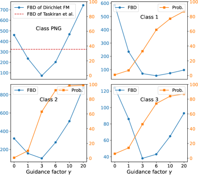
Figure 5: Classifier-free guidance for cell type conditional enhancer design. We generate enhancers that are only active in cell class via classifier-free guidance with varying $\gamma$. Shown are 4 classes of the Fly Brain cell data. The left y-axis FBD is computed between the generated sequences and the data distribution conditioned on the target class. For the first class, ”PNG”, functional sequences of Taskiran et al. (2023) are available, and we show their FBD. The right y-axis Prob. refers to the target class probability of a classifier for the generated sequences in percent.

Q1: How well can Dirichlet FM capture the sequence distribution? We compare with an autoregressive language model (the best baseline in the promoter design experiments in Section 4.2) and with Linear FM. To evaluate, we calculate the FBD between the models’ generated sequences and the unconditional data distribution. Dirichlet FM outperforms the language model by a large margin on both datasets and linear FM for human melanoma cell enhancer generation (Table 2). Moreover, distillation minimally impacts FBD while speeding up inference by 3 orders of magnitude compared to the language model and 2 to Dirichlet FM (distilled Dirichlet FM only requires 1 step). Such speedups, compared to autoregressive models, make Dirichlet FM a promising direction for other applications with high sequence lengths where inference times are important.

Q2: Can guided Dirichlet FM produce class-specific sequences and improve upon the state-of-the-art? We condition Dirichlet FM on different target cell-type classes via guidance (Section 3.4). To quantify how well the generated sequences match the target class distribution, we use the FBD between the generated distribution and the data distribution conditioned on the target class. Additionally, we train a separate cell-type classifier and evaluate the probability it assigns to the target class for a generated sequence.

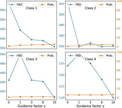
Figure 9: Evaluation for cell type specific enhancer design with classifier guidance. We condition Dirichlet FM to generate sequences that are only active in a class of cell type via classifier guidance with varying $\gamma$. Results are shown for 4 classes in the Fly Brain cell data. The left y-axis FBD is computed between the generated sequences and the data distribution conditioned on the target class. The right y-axis Prob. refers to the target class probability of a classifier for the generated sequences.

Sequences of classifier-free guided Dirichlet FM for the cell-type perineurial glia (PNG) have better FBD (Figure 5) than the sequences of Taskiran et al. (2023), of which several were experimentally validated as functioning enhancers (we show this comparison only for the PNG class since their sequences are available for it). For the other classes, guidance is similarly effective; by increasing the guidance factor $\gamma$, the classifier probability for generated sequences to belong to the target class can be improved close to 100%, and the FBD improves significantly until reaching a minimum (after the minimum the diversity decreases and the FBD worsens). The improvements with classifier guidance (Appendix Figure 9) are still significant but smaller.

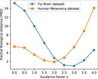
Figure 6: Classifier-free guidance for unconditional enhancer generation. We generate unconditional sequences with classifier-free guidance by sampling the target class based on its empirical frequency. We show the FBD between the generated data and the full data distribution for varying levels of guidance $\gamma$.

Q3: Can guidance improve unconditional generation? We generate unconditional sequences with classifier-free guided Dirichlet FM by first sampling a class (based on its empirical frequency) and then guiding toward that class. This significantly improves sample quality compared to unguided Dirichlet FM (Figure 6) and baselines (Table 2). Thus, guided Dirichlet FM via the connection we derive between flow and score reproduces the success in image diffusion models of enhancing sample quality via conditioning (Rombach et al., 2022; Saharia et al., 2022). Furthermore, like guidance for images (Xu et al., 2023), the FBD first improves under increased guidance (Figure 6) until reaching a minimum, after which increased guidance deteriorates sample diversity and, therefore, FBD.

5 Conclusion

We presented Dirichlet flow matching for modeling discrete data via a generative process on the simplex. This solves the pathological behavior of linear flow matching on the simplex, which we identified. Compared with autoregressive methods or diffusion with discrete noise, Dirichlet FM enables distillation and conditional generation via guidance, which we derived via a connection between the marginal flow and the scores of a mixture of Dirichlets.

Experimental results on important regulatory DNA sequence design tasks across 3 datasets demonstrate Dirichlet FM’s effectiveness and utility for hard generative modeling tasks over long sequences. The results confirm Dirichlet FM’s superiority to linear FM and multiple discrete diffusion approaches. Distilling Dirichlet FM only marginally impacts performance while enabling one-step generation, leading to multiple orders of magnitude speedups compared to autoregressive generative models for long sequences. Lastly, we demonstrated effective class conditional generation via guided Dirichlet FM to design cell-type specific enhancers - an important task for gene therapies. Hence, Dirichlet FM is a flexible framework (guidance, distillation) with strong performance for biological sequence generation and a promising direction for further discrete data applications.

Appendix A Method Details

Flow Matching with Cross-Entropy Loss

For all $t$ and $\mathbf{x}\in S_{K}$, at convergence our denoising classifier satisfies

$$\hat{p}(\mathbf{x}_{1}\mid\mathbf{x})=\frac{p_{t}(\mathbf{x}\mid\mathbf{x}_{1})p_{\text{data}}(\mathbf{x}_{1})}{p_{t}(\mathbf{x})}$$ (25)

Thus, if we parameterize the vector field via Equation 10, then we are assured that

$$\hat{v}(\mathbf{x},t;\theta)=\sum_{i=1}^{K}u_{t}(\mathbf{x}\mid\mathbf{x}_{1}=\mathbf{e}_{i})\frac{p_{t}(\mathbf{x}\mid\mathbf{x}_{1})p_{\text{data}}(\mathbf{x}_{1})}{p_{t}(\mathbf{x})}\quad=v(\mathbf{x},t;\theta)$$ (26)

Proof of Proposition 1

Proposition 1.

Suppose that a flow matching model is trained with the linear flow map (Equation 11). Then, for all $k=2,\ldots K$ and $\mathbf{x}\sim p_{t}(\mathbf{x})$, the converged model posterior $p(\mathbf{x}_{1}\mid\mathbf{x})\propto p_{t}(\mathbf{x}\mid\mathbf{x}_{1})p_{\text{data}}(\mathbf{x}_{1})$ has support over at most $k-1$ vertices for times $t>1/k$.

Proof.

In linear flow matching, the explicit form of the conditional probability path is given by

$$p_{t}(\mathbf{x}\mid\mathbf{x}_{1}=\mathbf{e}_{i})=\begin{cases}[(1-t)^{K-1}\Gamma(K)]^{-1}&x_{i}\geq t\\ 0&x_{i}<t\end{cases}$$ (27)

Suppose for sake of contradiction that $t>1/k$ but $p_{t}(\mathbf{x}\mid\mathbf{x}_{1})p_{\text{data}}(\mathbf{x}_{1})\neq 0$ for $k^{\prime}\geq k$ values of $\mathbf{x}_{1}$. Without loss of generality, suppose that $\mathbf{e}_{1},\ldots\mathbf{e}_{k}$ are $k$ of those values. Then, by Equation 27, we have $x_{i}\geq t$ for $i=1,\ldots k$. Then

$$\boldsymbol{1}^{T}\mathbf{x}=\sum_{i=1}^{K}x_{i}\geq\sum_{i=1}^{k}x_{i}\geq kt>k\cdot\frac{1}{k}=1$$ (28)

This contradicts the fact that $\mathbf{x}$ must lie on the simplex. ∎

A.1 Dirichlet Conditional Vector Field

As preliminaries, we recall the definition of the multivariate beta function:

$$\mathcal{B}(\alpha_{1},\ldots\alpha_{K})=\frac{\prod_{i=1}^{K}\Gamma(\alpha_{i})}{\Gamma\left(\sum_{i=1}^{K}\alpha_{i}\right)}$$ (29)

and that of the incomplete (two-argument) beta function:

$$\mathcal{B}(x;a,b)=\int_{0}^{x}t^{a-1}(1-t)^{b-1}\,dt$$ (30)

with the identity $\mathcal{B}(a,b)=\mathcal{B}(1;a,b)$.

We wish to construct a conditional flow $u_{t}(\mathbf{x}\mid\mathbf{x}_{1}=\mathbf{e}_{i})$ which generates the evolution of the conditional probability path

$$p_{t}(\mathbf{x}\mid\mathbf{x}_{1}=\mathbf{e}_{i})=\operatorname{Dir}(\mathbf{x};1,\ldots\alpha_{i}=1+t,\ldots 1)=\frac{\Gamma(t+K)}{\Gamma(t+1)}x_{i}^{t}$$ (31)

We choose the following ansatz for the functional form of $u_{t}$:

$$u_{t}(\mathbf{x}\mid\mathbf{x}_{1}=\mathbf{e}_{i})=C(x_{i},t)(\mathbf{e}_{i}-\mathbf{x})$$ (32)

i.e., (1) the flow points towards the target vertex $\mathbf{e}_{i}$ and (2) the magnitude is scaled by a constant dependent only on $x_{i}$ and $t$. Then consider the $(K-2)$-dimensional hyperplane $A_{b}$ of constant $x_{i}=b$ which cuts through the simplex, separating it into two regions $S_{1},S_{2}$ (Figure 7). We make the following key observation:

The probability flux crossing the plane $A_{b}$ is equal to the the rate of change of the total probability of region $S_{1}$.

Thus, we solve for the constant $C(x_{i},t)$ in the ansatz by deriving these two quantities and setting them equal to each other.

Figure 7: Conceptual derivation of the conditional vector field

Q1: What is the probability mass of $S_{1}$ and its rate of change?

The probability mass of $S_{1}$ can be obtained by integrating the density over each hyperplane $A_{c}$ (defined by $x_{i}=c$) for $c<b$ and then integrating over all such hyperplanes. Since the density is a constant proportional to $x_{i}^{t}=c^{t}$ over each hyperplane, we obtain

$$p_{t}(S_{1})\propto\int_{0}^{b}c^{t}\cdot\operatorname{Vol}(A_{c})\,dc$$ (33)

where $\operatorname{Vol}(A_{c})$ refers to the volume of the intersection between the hyperplane and the simplex. Since this region is defined by $x_{i}=c$, the remaining entries of $\mathbf{x}$ must add up to $1-c$. Thus, $A_{c}$ can be viewed as a nonstandard probability simplex over $K-1$ variables. The volume of this $(K-2)$-dimensional space is proportional to $(1-c)^{K-2}$, giving

$$\rho(S_{1})\propto\int_{0}^{b}c^{t}(1-c)^{K-2}\,dc=\mathcal{B}(b;t+1,K-1)$$ (34)

Normalizing, we obtain

$$p_{t}(S_{1})=\frac{\int_{0}^{b}c^{t}(1-c)^{K-2}\,dc}{\int_{0}^{1}c^{t}(1-c)^{K-2}\,dc}=\frac{\mathcal{B}(b;t+1,K-1)}{\mathcal{B}(t+1,K-1)}=I_{b}(t+1,K-1)$$ (35)

where $I$ is the so-called regularized incomplete beta function and is well-known as the CDF of the Beta distribution. Its derivative with respect to the first parameter is not available in closed form, but we write it as

$$\tilde{I}_{x}(a,b)=\frac{\partial}{\partial a}I_{x}(a,b)=\frac{\partial}{\partial a}\frac{\mathcal{B}(x;a,b)}{\mathcal{B}(a,b)}$$ (36)

and thus obtain the rate of change of $p_{t}(S_{1})$ as $\tilde{I}_{b}(t+1,K-1)$.

Q2: What is the probability flux across the hyperplane $A_{b}$? The probability flux across $A_{b}$ (into $S_{2}$) is given by

$$J=\iint_{A_{b}}u_{t}p_{t}\cdot\mathbf{\hat{n}}\,dA=\iint_{A_{b}}p_{t}\cdot C(b,t)(\mathbf{e}_{i}-\mathbf{x})\cdot\frac{\mathbf{n}}{\lVert\mathbf{n}\rVert}\,dA$$ (37)

The normal vector $\mathbf{n}$ points from the center of the face opposite $\mathbf{e}_{i}$, specified by $x_{i}=0$ and $x_{j}=1/(K-1),j\neq i$, towards $\mathbf{e}_{i}$. Thus, the probability flux density is given by the dot product of

$$\mathbf{e}_{i}-\mathbf{x} =(-x_{1},\ldots\mathbf{x}_{i}=1-b,\ldots-x_{K})$$ (38)

$$\mathbf{n} =\left(-\frac{1}{K-1},\ldots\mathbf{x}_{i}=1,\ldots-\frac{1}{K-1}\right)$$

Since $\sum_{j\neq i}x_{j}=1-b$, this dot product is equal to $(1-b)K/(K-1)$. We also see that $\lVert\mathbf{n}\rVert=\sqrt{K/(K-1)}$. Importantly, the flux density is constant on the hyperplane $A$, so the total flux is given by a simple product:

$$J =C(b,t)\cdot p_{t}\cdot(1-b)\sqrt{\frac{K}{K-1}}\operatorname{Vol}(A_{b})$$ (39)

$$=C(b,t)\cdot\left[\frac{1}{\sqrt{K}}\frac{\Gamma(t+K)}{\Gamma(t+1)}b^{t}\right](1-b)\sqrt{\frac{K}{K-1}}\frac{\sqrt{K-1}}{\Gamma(K-1)}(1-b)^{K-2}$$ (40)

$$=C(b,t)\cdot\frac{(1-b)^{K-1}b^{t}}{\mathcal{B}(t+1,K-1)}$$ (41)

where (for this step only) we note that the volume of a simplex over $K$ variables viewed as a subset of $\mathbb{R}^{K}$ is $\sqrt{K}/\Gamma(K)$, giving the Dirichlet PDF an additional factor of $1/\sqrt{K}$. Now setting $J=-\partial_{t}p_{t}(S_{1})$ from above, we obtain

$$C(b,t)=-\tilde{I}_{b}(t+1,K-1)\frac{\mathcal{B}(t+1,K-1)}{(1-b)^{K-1}b^{t}}$$ (42)

Checking the transport equation. We check that $\nabla\cdot(p_{t}u_{t})=-\partial p_{t}/\partial t$:

$$\nabla\cdot(p_{t}u_{t}) =-\nabla\cdot\left[\frac{\Gamma(t+K)}{\Gamma(t+1)}x_{i}^{t}\cdot\tilde{I}_{x_{i}}(t+1,K-1)\frac{\mathcal{B}(t+1,K-1)}{(1-x_{i})^{K-1}x_{i}^{t}}(\mathbf{e}_{i}-\mathbf{x})\right]$$ (43)

$$=-\Gamma(K-1)\nabla\cdot\left[\frac{\tilde{I}_{x_{i}}(t+1,K-1)}{(1-x_{i})^{K-1}}(\mathbf{e}_{i}-\mathbf{x})\right]$$ (44)

$$=-\Gamma(K-1)\left[\frac{\tilde{I}_{x_{i}}(t+1,K-1)}{(1-x_{i})^{K-1}}\nabla\cdot(\mathbf{e}_{i}-\mathbf{x})+(\mathbf{e}_{i}-\mathbf{x})\cdot\nabla\frac{\tilde{I}_{x_{i}}(t+1,K-1)}{(1-x_{i})^{K-1}}\right]$$ (45)

The divergence of $$\mathbf{x} (K-1) S_{K} K-1 x_{i} x_{i}$$ on the -dimensional space is . Also, the gradient of a function dependently only on has nonzero component only in the direction.

$$=-\Gamma(K-1)\left[\frac{\tilde{I}_{x_{i}}(t+1,K-1)}{(1-x_{i})^{K-1}}(1-K)+(1-x_{i})\frac{\partial}{\partial x_{i}}\frac{\tilde{I}_{x_{i}}(t+1,K-1)}{(1-x_{i})^{K-1}}\right]$$ (46)

$$=-\Gamma(K-1)\left[\frac{\tilde{I}_{x_{i}}(t+1,K-1)}{(1-x_{i})^{K-1}}(1-K)+(1-x_{i})\left(\tilde{I}_{x_{i}}\frac{K-1}{(1-x_{i})^{K}}+\frac{1}{(1-x_{i})^{K-1}}\frac{\partial\tilde{I}_{x_{i}}}{\partial x_{i}}\right)\right]$$ (47)

The first and second terms now cancel.

$$=-\Gamma(K-1)\left[\frac{1}{(1-x_{i})^{K-2}}\frac{\partial}{\partial x_{i}}\tilde{I}_{x_{i}}(t+1,K-1)\right]$$ (48)

Substituting Equation 36 and interchanging the order of derivatives,

$$=-\Gamma(K-1)\left[\frac{1}{(1-x_{i})^{K-2}}\frac{\partial}{\partial t}\frac{1}{\mathcal{B}(t+1,K-1)}\frac{\partial}{\partial x_{i}}\mathcal{B}(x_{i};t+1,K-1)\right]$$ (49)

$$=-\frac{1}{(1-x_{i})^{K-2}}\frac{\partial}{\partial t}\frac{\Gamma(K-1)}{\mathcal{B}(t+1,K-1)}x_{i}^{t}(1-x_{i})^{K-2}$$ (50)

$$=-\frac{\partial}{\partial t}\frac{\Gamma(t+K)}{\Gamma(t+1)}x_{i}^{t}\quad=-\frac{\partial p_{t}}{\partial t}$$ (51)

Appendix B Experimental details

B.1 Training and Inference

Algorithm 1 Training for a single simplex. For a discrete data sequence, this extends to a sequence of simplices.

  Input: Discrete training one-hot vectors $\{\mathbf{x}_{j}\}$, neural network $\phi$

  for all $\mathbf{x}_{j}$ do

     Sample $t\sim\mathcal{U}[0,1]$

     Sample $\mathbf{x}_{t}\sim p_{t}(\mathbf{x}_{t}\mid\mathbf{x}=\mathbf{e}_{i})$ where $p_{t}(\mathbf{x}_{t}\mid\mathbf{x}=\mathbf{e}_{i})=\operatorname{Dir}(\mathbf{x};\boldsymbol{\alpha}=\boldsymbol{1}+t\cdot\mathbf{e}_{i})$

     Predict $\hat{\mathbf{p}}\leftarrow\phi(\mathbf{x}_{t},t)$

     Optimize loss $\mathcal{L}=\mathbf{CrossEntropy}(\hat{\mathbf{p}},\mathbf{x})$

  end for

Algorithm 2 Inference for a single simplex. For a discrete data sequence, this extends to a sequence of simplices.

  Input: Trained neural network $\phi$. Number of integration steps $N$

  Sample $\mathbf{x}_{0}\sim\operatorname{Dir}(\mathbf{x};\boldsymbol{1}$

  Set $\mathbf{x}_{t}\leftarrow\mathbf{x}_{0}$

  for $n\leftarrow 0$ to $N-1$ do

     Let $t\leftarrow n/N$ 

     Predict $\hat{\mathbf{p}}\leftarrow\phi(\mathbf{x}_{t},t)$  

     Calculate conditional vector fields $u_{t}(\mathbf{x}_{t}\mid\mathbf{x}_{1}=\mathbf{e}_{i})=\tilde{I}_{x_{i}}(t+1,K-1)\frac{\mathcal{B}(t+1,K-1)}{(1-x_{i})^{K-1}x_{i}^{t}}(\mathbf{e}_{i}-\mathbf{x}_{t})$ 

     Calculate marginal vector field $u_{t}(\mathbf{x}_{t})=\sum_{i=0}^{K}\hat{\mathbf{p}}_{i}u_{t}(\mathbf{x}_{t}\mid\mathbf{x}_{1}=\mathbf{e}_{i})$ 

     Take step $\mathbf{x}_{t}\leftarrow\mathbf{x}_{t}+\frac{n}{N}\cdot\mathbf{x}_{t}$  

  end for

  return $\mathbf{x}_{t}$

We provide algorithms for training and inference in Algorithm 1, and Algorithm 2. These describe the procedures for generating discrete data on a single simplex. When generating a discrete data sequence, they are extended easily by performing the same procedure for a sequence of simplices. Code for reproducing all results is available in the accompanying supplementary material as .zip file.

Toy experiments. We train all models in Figure 4 for 450,000 steps with a batch size of 512 to ensure that they have all converged and then evaluate the KL of the final step.

Promoter Design. We follow the setup of Avdeyev et al. (2023) and train for 200 epochs with a learning rate of $5\times 10^{-4}$ and early stopping on the MSE on the validation set. We communicated with Avdeyev et al. (2023) to ensure that we have the same training and inference setup as them, and we build on their codebase to evaluate the generated sequences with the Sei regulatory activity prediction model (Chen et al., 2022). Thus, we use 100 inference steps for our Dirichlet FM instead of the 400 that they use in their code since they state that they used 100 integration steps for the results in the paper, which is also stated in the paper. Under this setup, we obtain the performance numbers for Linear FM and Dirichlet FM. We also ran the autoregressive language model in this setup (except for the number of inference steps which does not apply). Meanwhile, the numbers we report for Bit Diffusion, D3PM, and DDSM are taken from the DDSM paper (Avdeyev et al., 2023).

Enhancer Design. For both evaluations, on the human melanoma cell and the fly brain cell dataset, we train for 800 epochs (convergence of validation curves is reached after approximately 300 for both datasets). We use FBD for early stopping. For inference, we use 100 integration steps.

Classifier-free Guidance. For classifier-free guidance, we train with a conditioning ratio (the fraction of times we train with a class label as input instead of the no-class token as input) of 0.7. During inference, the inference Algorithm 2 is changed in that two probability vectors $\hat{\mathbf{p}}$ are predicted, once with class conditioning and once without class conditioning, which we sum together according to Equation 22. Then, we project the resulting probabilities onto the simplex since negative values can arise for guidance factors $\gamma>1$. For this purpose, we use the algorithm by Wang & Carreira-Perpinán (2013).

Classifier Guidance. The noisy classifier that we train for classifier guidance has the same architecture as our generative model, except that we sum the final representations and feed them into a 2-layer feed-forward network that serves as classification head. For training, we use early stopping on the accuracy and train for approximately 800 epochs. During inference, we use automatic differentiation to obtain the classifier’s gradients with respect to the input points on the simplices. To perform classifier guidance, we then convert the flow model output probabilities to scores as described in Section 3.4, obtain the guided score by adding the unconditional and the conditional scores via Equation 23, and convert the obtained scores back to probabilities. These we project to the simplex (Wang & Carreira-Perpinán, 2013) from which we obtain the vector field for integration.

Classifier for FBD calculation. This classifier’s architecture is similar to that of the noisy classifier for classifier guidance. However, it does not have any time conditioning and takes token embeddings as input instead of points on the simplex. For training, we use early stopping on the accuracy and train approximately 100 epochs.

The sequence embeddings that we use to calculate FBD are given by the hidden features after the first layer of the classification head. The 4 classes that we choose for the cell type specific enhancer generation are chosen as classes with a good tradeoff between the area under the receiver operator characteristic curve and the area under the precision-recall curve.

Distillation. For distillation, we run inference with the teacher model for every training step of the student model to obtain pairs of noise and training targets. With this, we train the student model on approximately 6 billion sequences.

Computational requirements. We train on RTX A600 GPUs. Training in the enhancer generation setup for 200 epochs on sequences with length 500 takes 7 hours. Our largest model uses approximately 8GB of RAM during training.

Architecture The architecture that we use for the promoter design experiments is the same as in DDSM (Avdeyev et al., 2023). In our other experiments we replaced group norm with layer norm in their architecture. The model consists of 20 layers of 1D convolutions interleaved with time embedding layers (and class-type embedding layers for classifier-free guidance) and normalization layers. We also experimented with Transformer architectures, which led to worse performance. All models use this 20-layer architecture except for the classifier for the Fly Brain data, which has 5 layers.

B.2 Data

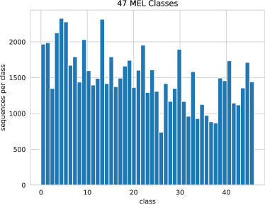
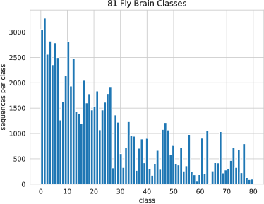
Figure 8: Histograms of cell type classes for fly brain cell enhancer sequence data and human melanoma cell data.

For the enhancer data of 104665 fly brain cell sequences (Janssens et al., 2022), we use the same split as Taskiran et al. (2023), resulting in an 83726/10505/10434 split for train/val/test. Meanwhile, for the human melanoma cell dataset of 88870 sequences (Atak et al., 2021), their split has 70892/8966/9012 sequences. It is noteworthy that these datasets contain ATAC-seq data (Buenrostro et al., 2013), which means that not all sequences are guaranteed to be enhancers and actually enhance transcription of a certain gene. ATAC-seq only measures the chromatin accessibility of the sequences in the cell types, which is a necessary but not sufficient requirement for a sequence to be an enhancer. In Figure 8, we show histograms for the class distributions of both datasets. For the melanoma dataset, there is little class imbalance.

Appendix C Additional Results

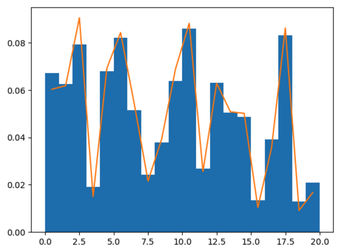
Figure 10: Simulation results for classifier guidance on a conditional categorical distribution with an analytically tractable vector field. In blue, we show a histogram (with frequencies normalized to density) of the generated classes for each class on the x-axis. In orange, we show the true probabilities of the toy distribution conditioned on the same class that we use for classifier guidance.

Analytical toy experiment for classifier guidance. As a toy experiment to demonstrate our classifier guidance procedure, we construct a distribution conditioned on a binary random variable. The conditional distribution is a categorical distribution over 20 classes. In this setup, the time-dependent class probabilities conditioned on a noisy point on the simplex can be computed analytically. Thus, we can use them to obtain the vector field for Dirichlet FM analytically. Furthermore, the class probabilities and the gradients of their logarithm (the score) can be computed analytically. Hence, we can simulate classifier guided Dirichlet FM analytically for this toy distribution.

The results in Figure 10 show a close match between the empirical distribution of the generated data and the ground truth probabilities. This empirically confirms the effectiveness of our classifier guidance procedure that relies on converting probabilities to scores and converting them back to probabilities by solving a linear system of equations.

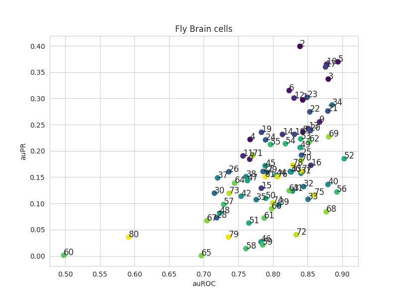
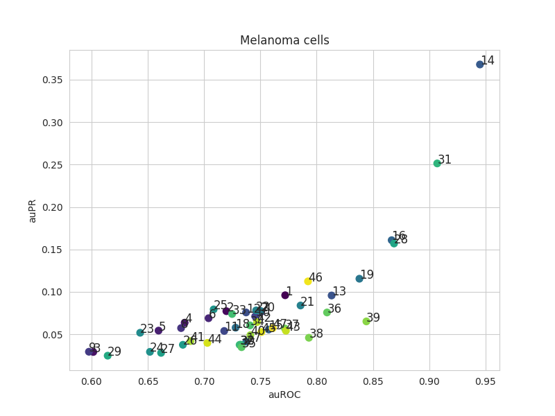
Figure 11: Per class performance of the classifiers used for evaluation and FBD calculation. Shown are scatter plots for each class of the fly brain data (left) and the human melanoma cell data (right) between the area under the curve of the receiver operator characteristic (x-axis) and the area under the precision-recall curve (y-axis). The scatter plots match the results of the classifiers of Atak et al. (2021) and Janssens et al. (2022) closely.

References

- Albergo & Vanden-Eijnden (2022) Albergo, M. S. and Vanden-Eijnden, E. Building normalizing flows with stochastic interpolants. In The Eleventh International Conference on Learning Representations, 2022.
- Atak et al. (2021) Atak, Z. K., Taskiran, I. I., Demeulemeester, J., Flerin, C., Mauduit, D., Minnoye, L., Hulselmans, G., Christiaens, V., Ghanem, G.-E., Wouters, J., and Aerts, S. Interpretation of allele-specific chromatin accessibility using cell state-aware deep learning. Genome Res., 2021.
- Austin et al. (2021) Austin, J., Johnson, D. D., Ho, J., Tarlow, D., and Van Den Berg, R. Structured denoising diffusion models in discrete state-spaces. Advances in Neural Information Processing Systems, 2021.
- Avdeyev et al. (2023) Avdeyev, P., Shi, C., Tan, Y., Dudnyk, K., and Zhou, J. Dirichlet diffusion score model for biological sequence generation. arXiv preprint arXiv:2305.10699, 2023.
- Bose et al. (2023) Bose, A. J., Akhound-Sadegh, T., Fatras, K., Huguet, G., Rector-Brooks, J., Liu, C.-H., Nica, A. C., Korablyov, M., Bronstein, M., and Tong, A. Se (3)-stochastic flow matching for protein backbone generation. arXiv preprint arXiv:2310.02391, 2023.
- Buenrostro et al. (2013) Buenrostro, J. D., Giresi, P. G., Zaba, L. C., Chang, H. Y., and Greenleaf, W. J. Transposition of native chromatin for fast and sensitive epigenomic profiling of open chromatin, dna-binding proteins and nucleosome position. Nature Methods, 2013.
- Campbell et al. (2022) Campbell, A., Benton, J., De Bortoli, V., Rainforth, T., Deligiannidis, G., and Doucet, A. A continuous time framework for discrete denoising models. Advances in Neural Information Processing Systems, 35:28266–28279, 2022.
- Chen et al. (2022) Chen, K. M., Wong, A. K., Troyanskaya, O. G., and Zhou, J. A sequence-based global map of regulatory activity for deciphering human genetics. Nature Genetics, 2022.
- Chen & Lipman (2023) Chen, R. T. and Lipman, Y. Riemannian flow matching on general geometries. arXiv preprint arXiv:2302.03660, 2023.
- Chen et al. (2023) Chen, T., ZHANG, R., and Hinton, G. Analog bits: Generating discrete data using diffusion models with self-conditioning. In The Eleventh International Conference on Learning Representations, 2023.
- Dao et al. (2023) Dao, Q., Phung, H., Nguyen, B., and Tran, A. Flow matching in latent space. arXiv preprint arXiv:2307.08698, 2023.
- de Almeida et al. (2023) de Almeida, B. P., Schaub, C., Pagani, M., Secchia, S., Furlong, E. E. M., and Stark, A. Targeted design of synthetic enhancers for selected tissues in the drosophila embryo. Nature, 2023.
- Dhariwal & Nichol (2021) Dhariwal, P. and Nichol, A. Diffusion models beat gans on image synthesis. Advances in neural information processing systems, 34:8780–8794, 2021.
- Dieleman et al. (2022) Dieleman, S., Sartran, L., Roshannai, A., Savinov, N., Ganin, Y., Richemond, P. H., Doucet, A., Strudel, R., Dyer, C., Durkan, C., et al. Continuous diffusion for categorical data. arXiv preprint arXiv:2211.15089, 2022.
- Dunham et al. (2012) Dunham, I., Kundaje, A., Aldred, S. F., Collins, P. J., Davis, C. A., Doyle, F., Epstein, C. B., Frietze, S., Harrow, J., Kaul, R., Khatun, J., Lajoie, B. R., Landt, S. G., Lee, B.-K., Pauli, F., Rosenbloom, K. R., Sabo, P., Safi, A., Sanyal, A., Shoresh, N., Simon, J. M., Song, L., Trinklein, N. D., Altshuler, R. C., Birney, E., Brown, J. B., Cheng, C., Djebali, S., Dong, X., Ernst, J., Furey, T. S., Gerstein, M., Giardine, B., Greven, M., Hardison, R. C., Harris, R. S., Herrero, J., Hoffman, M. M., Iyer, S., Kellis, M., Kheradpour, P., Lassmann, T., Li, Q., Lin, X., Marinov, G. K., Merkel, A., Mortazavi, A., Parker, S. C. J., Reddy, T. E., Rozowsky, J., Schlesinger, F., Thurman, R. E., Wang, J., Ward, L. D., Whitfield, T. W., Wilder, S. P., Wu, W., Xi, H. S., Yip, K. Y., Zhuang, J., Bernstein, B. E., Green, E. D., Gunter, C., Snyder, M., Pazin, M. J., Lowdon, R. F., Dillon, L. A. L., Adams, L. B., Kelly, C. J., Zhang, J., Wexler, J. R., Good, P. J., Feingold, E. A., Crawford, G. E., Dekker, J., Elnitski, L., Farnham, P. J., Giddings, M. C., Gingeras, T. R., Guigó, R., Hubbard, T. J., Kent, W. J., Lieb, J. D., Margulies, E. H., Myers, R. M., Stamatoyannopoulos, J. A., Tenenbaum, S. A., Weng, Z., White, K. P., Wold, B., Yu, Y., Wrobel, J., Risk, B. A., Gunawardena, H. P., Kuiper, H. C., Maier, C. W., Xie, L., Chen, X., Mikkelsen, T. S., Gillespie, S., Goren, A., Ram, O., Zhang, X., Wang, L., Issner, R., Coyne, M. J., Durham, T., Ku, M., Truong, T., Eaton, M. L., Dobin, A., Tanzer, A., Lagarde, J., Lin, W., Xue, C., Williams, B. A., Zaleski, C., Röder, M., Kokocinski, F., Abdelhamid, R. F., Alioto, T., Antoshechkin, I., Baer, M. T., Batut, P., Bell, I., Bell, K., Chakrabortty, S., Chrast, J., Curado, J., Derrien, T., Drenkow, J., Dumais, E., Dumais, J., Duttagupta, R., Fastuca, M., Fejes-Toth, K., Ferreira, P., Foissac, S., Fullwood, M. J., Gao, H., Gonzalez, D., Gordon, A., Howald, C., Jha, S., Johnson, R., Kapranov, P., King, B., Kingswood, C., Li, G., Luo, O. J., Park, E., Preall, J. B., Presaud, K., Ribeca, P., Robyr, D., Ruan, X., Sammeth, M., Sandhu, K. S., Schaeffer, L., See, L.-H., Shahab, A., Skancke, J., Suzuki, A. M., Takahashi, H., Tilgner, H., Trout, D., Walters, N., Wang, H., Hayashizaki, Y., Reymond, A., Antonarakis, S. E., Hannon, G. J., Ruan, Y., Carninci, P., Sloan, C. A., Learned, K., Malladi, V. S., Wong, M. C., Barber, G. P., Cline, M. S., Dreszer, T. R., Heitner, S. G., Karolchik, D., Kirkup, V. M., Meyer, L. R., Long, J. C., Maddren, M., Raney, B. J., Grasfeder, L. L., Giresi, P. G., Battenhouse, A., Sheffield, N. C., Showers, K. A., London, D., Bhinge, A. A., Shestak, C., Schaner, M. R., Ki Kim, S., Zhang, Z. Z., Mieczkowski, P. A., Mieczkowska, J. O., Liu, Z., McDaniell, R. M., Ni, Y., Rashid, N. U., Kim, M. J., Adar, S., Zhang, Z., Wang, T., Winter, D., Keefe, D., Iyer, V. R., Zheng, M., Wang, P., Gertz, J., Vielmetter, J., Partridge, E., Varley, K. E., and Gasper, C. An integrated encyclopedia of dna elements in the human genome. Nature, 2012.
- Floto et al. (2023) Floto, G., Jonsson, T., Nica, M., Sanner, S., and Zhu, E. Z. Diffusion on the probability simplex. arXiv preprint arXiv:2309.02530, 2023.
- Forrest et al. (2014) Forrest, A. R. R., Kawaji, H., Rehli, M., Kenneth Baillie, J., de Hoon, M. J. L., Haberle, V., Lassmann, T., Kulakovskiy, I. V., Lizio, M., Itoh, M., Andersson, R., Mungall, C. J., Meehan, T. F., Schmeier, S., Bertin, N., Jørgensen, M., Dimont, E., Arner, E., Schmidl, C., Schaefer, U., Medvedeva, Y. A., Plessy, C., Vitezic, M., Severin, J., Semple, C. A., Ishizu, Y., Young, R. S., Francescatto, M., Alam, I., Albanese, D., Altschuler, G. M., Arakawa, T., Archer, J. A. C., Arner, P., Babina, M., Rennie, S., Balwierz, P. J., Beckhouse, A. G., Pradhan-Bhatt, S., Blake, J. A., Blumenthal, A., Bodega, B., Bonetti, A., Briggs, J., Brombacher, F., Maxwell Burroughs, A., Califano, A., Cannistraci, C. V., Carbajo, D., Chen, Y., Chierici, M., Ciani, Y., Clevers, H. C., Dalla, E., Davis, C. A., Detmar, M., Diehl, A. D., Dohi, T., Drabløs, F., Edge, A. S. B., Edinger, M., Ekwall, K., Endoh, M., Enomoto, H., Fagiolini, M., Fairbairn, L., Fang, H., Farach-Carson, M. C., Faulkner, G. J., Favorov, A. V., Fisher, M. E., Frith, M. C., Fujita, R., Fukuda, S., Furlanello, C., Furuno, M., Furusawa, J.-i., Geijtenbeek, T. B., Gibson, A. P., Gingeras, T., Goldowitz, D., Gough, J., Guhl, S., Guler, R., Gustincich, S., Ha, T. J., Hamaguchi, M., Hara, M., Harbers, M., Harshbarger, J., Hasegawa, A., Hasegawa, Y., Hashimoto, T., Herlyn, M., Hitchens, K. J., Ho Sui, S. J., Hofmann, O. M., Hoof, I., Hori, F., Huminiecki, L., Iida, K., Ikawa, T., Jankovic, B. R., Jia, H., Joshi, A., Jurman, G., Kaczkowski, B., Kai, C., Kaida, K., Kaiho, A., Kajiyama, K., Kanamori-Katayama, M., Kasianov, A. S., Kasukawa, T., Katayama, S., Kato, S., Kawaguchi, S., Kawamoto, H., Kawamura, Y. I., Kawashima, T., Kempfle, J. S., Kenna, T. J., Kere, J., Khachigian, L. M., Kitamura, T., Peter Klinken, S., Knox, A. J., Kojima, M., Kojima, S., Kondo, N., Koseki, H., Koyasu, S., Krampitz, S., Kubosaki, A., Kwon, A. T., Laros, J. F. J., Lee, W., Lennartsson, A., Li, K., Lilje, B., Lipovich, L., Mackay-sim, A., Manabe, R.-i., Mar, J. C., Marchand, B., Mathelier, A., Mejhert, N., Meynert, A., Mizuno, Y., de Lima Morais, D. A., Morikawa, H., Morimoto, M., Moro, K., Motakis, E., Motohashi, H., Mummery, C. L., Murata, M., Nagao-Sato, S., Nakachi, Y., Nakahara, F., Nakamura, T., Nakamura, Y., Nakazato, K., van Nimwegen, E., Ninomiya, N., Nishiyori, H., Noma, S., Nozaki, T., Ogishima, S., Ohkura, N., Ohmiya, H., Ohno, H., Ohshima, M., Okada-Hatakeyama, M., Okazaki, Y., Orlando, V., Ovchinnikov, D. A., Pain, A., Passier, R., Patrikakis, M., Persson, H., Piazza, S., Prendergast, J. G. D., Rackham, O. J. L., Ramilowski, J. A., Rashid, M., Ravasi, T., Rizzu, P., Roncador, M., Roy, S., Rye, M. B., Saijyo, E., Sajantila, A., Saka, A., Sakaguchi, S., Sakai, M., Sato, H., Satoh, H., Savvi, S., Saxena, A., Schneider, C., Schultes, E. A., Schulze-Tanzil, G. G., Schwegmann, A., Sengstag, T., Sheng, G., Shimoji, H., Shimoni, Y., Shin, J. W., Simon, C., Sugiyama, D., Sugiyama, T., Suzuki, M., Suzuki, N., Swoboda, R. K., ’t Hoen, P. A. C., Tagami, M., Takahashi, N., Takai, J., Tanaka, H., Tatsukawa, H., Tatum, Z., Thompson, M., Toyoda, H., Toyoda, T., Valen, E., van de Wetering, M., van den Berg, L. M., Verardo, R., Vijayan, D., Vorontsov, I. E., Wasserman, W. W., Watanabe, S., Wells, C. A., Winteringham, L. N., Wolvetang, E., Wood, E. J., Yamaguchi, Y., Yamamoto, M., Yoneda, M., Yonekura, Y., Yoshida, S., Zabierowski, S. E., Zhang, P. G., Zhao, X., Zucchelli, S., Summers, K. M., Suzuki, H., Daub, C. O., Kawai, J., Heutink, P., Hide, W., Freeman, T. C., Lenhard, B., Bajic, V. B., Taylor, M. S., Makeev, V. J., Sandelin, A., Hume, D. A., Carninci, P., Hayashizaki, Y., Consortium, T. F., the RIKEN PMI, and (DGT), C. A promoter-level mammalian expression atlas. Nature, 2014.
- Frey et al. (2024) Frey, N. C., Berenberg, D., Zadorozhny, K., Kleinhenz, J., Lafrance-Vanasse, J., Hotzel, I., Wu, Y., Ra, S., Bonneau, R., Cho, K., Loukas, A., Gligorijevic, V., and Saremi, S. Protein discovery with discrete walk-jump sampling. In The Twelfth International Conference on Learning Representations, 2024.
- Haberle & Stark (2018) Haberle, V. and Stark, A. Eukaryotic core promoters and the functional basis of transcription initiation. Nat. Rev. Mol. Cell Biol., 2018.
- Han et al. (2022) Han, X., Kumar, S., and Tsvetkov, Y. Ssd-lm: Semi-autoregressive simplex-based diffusion language model for text generation and modular control. arXiv preprint arXiv:2210.17432, 2022.
- Heusel et al. (2017) Heusel, M., Ramsauer, H., Unterthiner, T., Nessler, B., and Hochreiter, S. Gans trained by a two time-scale update rule converge to a local nash equilibrium. Advances in Neural Information Processing Systems, 2017.
- Ho & Salimans (2022) Ho, J. and Salimans, T. Classifier-free diffusion guidance. arXiv preprint arXiv:2207.12598, 2022.
- Hon et al. (2017) Hon, C.-C., Ramilowski, J. A., Harshbarger, J., Bertin, N., Rackham, O. J. L., Gough, J., Denisenko, E., Schmeier, S., Poulsen, T. M., Severin, J., Lizio, M., Kawaji, H., Kasukawa, T., Itoh, M., Burroughs, A. M., Noma, S., Djebali, S., Alam, T., Medvedeva, Y. A., Testa, A. C., Lipovich, L., Yip, C.-W., Abugessaisa, I., Mendez, M., Hasegawa, A., Tang, D., Lassmann, T., Heutink, P., Babina, M., Wells, C. A., Kojima, S., Nakamura, Y., Suzuki, H., Daub, C. O., de Hoon, M. J. L., Arner, E., Hayashizaki, Y., Carninci, P., and Forrest, A. R. R. An atlas of human long non-coding rnas with accurate 5 ends. Nature, 2017.
- Hoogeboom et al. (2021) Hoogeboom, E., Gritsenko, A. A., Bastings, J., Poole, B., Berg, R. v. d., and Salimans, T. Autoregressive diffusion models. arXiv preprint arXiv:2110.02037, 2021.
- Igashov et al. (2024) Igashov, I., Schneuing, A., Segler, M., Bronstein, M., and Correia, B. Retrobridge: Modeling retrosynthesis with markov bridges. In The Twelfth International Conference on Learning Representations, 2024.
- Janssens et al. (2022) Janssens, J., Aibar, S., Taskiran, I. I., Ismail, J. N., Gomez, A. E., Aughey, G., Spanier, K. I., De Rop, F. V., González-Blas, C. B., Dionne, M., Grimes, K., Quan, X. J., Papasokrati, D., Hulselmans, G., Makhzami, S., De Waegeneer, M., Christiaens, V., Southall, T., and Aerts, S. Decoding gene regulation in the fly brain. Nature, 2022.
- Li et al. (2023) Li, Z., Ni, Y., Huygelen, T., Das, A., Xia, G., Stan, G.-B., and Zhao, Y. Latent diffusion model for DNA sequence generation. In NeurIPS 2023 AI for Science Workshop, 2023.
- Lipman et al. (2022) Lipman, Y., Chen, R. T., Ben-Hamu, H., Nickel, M., and Le, M. Flow matching for generative modeling. In The Eleventh International Conference on Learning Representations, 2022.
- Liu et al. (2022) Liu, X., Gong, C., and Liu, Q. Flow straight and fast: Learning to generate and transfer data with rectified flow. arXiv preprint arXiv:2209.03003, 2022.
- Luo et al. (2020) Luo, Y., Hitz, B. C., Gabdank, I., Hilton, J. A., Kagda, M. S., Lam, B., Myers, Z., Sud, P., Jou, J., Lin, K., Baymuradov, U. K., Graham, K., Litton, C., Miyasato, S. R., Strattan, J. S., Jolanki, O., Lee, J.-W., Tanaka, F. Y., Adenekan, P., O’Neill, E., and Cherry, J. M. New developments on the encyclopedia of dna elements encode data portal. Nucleic Acids Res., 2020.
- Panigrahi & O’Malley (2021) Panigrahi, A. and O’Malley, B. W. Mechanisms of enhancer action: the known and the unknown. Genome Biology, 2021.
- Penzar et al. (2023) Penzar, D., Nogina, D., Noskova, E., Zinkevich, A., Meshcheryakov, G., Lando, A., Rafi, A. M., de Boer, C., and Kulakovskiy, I. V. LegNet: a best-in-class deep learning model for short DNA regulatory regions. Bioinformatics, 39, 2023.
- Pooladian et al. (2023) Pooladian, A.-A., Ben-Hamu, H., Domingo-Enrich, C., Amos, B., Lipman, Y., and Chen, R. Multisample flow matching: Straightening flows with minibatch couplings. arXiv preprint arXiv:2304.14772, 2023.
- Preuer et al. (2018) Preuer, K., Renz, P., Unterthiner, T., Hochreiter, S., and Klambauer, G. Fréchet chemnet distance: A metric for generative models for molecules in drug discovery. Journal of Chemical Information and Modeling, 2018.
- Richemond et al. (2022) Richemond, P. H., Dieleman, S., and Doucet, A. Categorical sdes with simplex diffusion. arXiv preprint arXiv:2210.14784, 2022.
- Rombach et al. (2022) Rombach, R., Blattmann, A., Lorenz, D., Esser, P., and Ommer, B. High-resolution image synthesis with latent diffusion models. In Proceedings of the IEEE/CVF Conference on Computer Vision and Pattern Recognition, 2022.
- Saharia et al. (2022) Saharia, C., Chan, W., Saxena, S., Li, L., Whang, J., Denton, E., Ghasemipour, S. K. S., Gontijo-Lopes, R., Ayan, B. K., Salimans, T., Ho, J., Fleet, D. J., and Norouzi, M. Photorealistic text-to-image diffusion models with deep language understanding. In Advances in Neural Information Processing Systems, 2022.
- Salimans & Ho (2022) Salimans, T. and Ho, J. Progressive distillation for fast sampling of diffusion models. In International Conference on Learning Representations, 2022.
- Shiraki et al. (2003) Shiraki, T., Kondo, S., Katayama, S., Waki, K., Kasukawa, T., Kawaji, H., Kodzius, R., Watahiki, A., Nakamura, M., Arakawa, T., Fukuda, S., Sasaki, D., Podhajska, A., Harbers, M., Kawai, J., Carninci, P., and Hayashizaki, Y. Cap analysis gene expression for high-throughput analysis of transcriptional starting point and identification of promoter usage. Proc. Natl. Acad. Sci. U. S. A., 2003.
- Song & Ermon (2019) Song, Y. and Ermon, S. Generative modeling by estimating gradients of the data distribution. Advances in neural information processing systems, 32, 2019.
- Song et al. (2021) Song, Y., Sohl-Dickstein, J., Kingma, D. P., Kumar, A., Ermon, S., and Poole, B. Score-based generative modeling through stochastic differential equations. In International Conference on Learning Representations, 2021.
- Song et al. (2023) Song, Y., Dhariwal, P., Chen, M., and Sutskever, I. Consistency models. Proceedings of the 40th International Conference on Machine Learning, pp. 32211–32252, 2023.
- Taskiran et al. (2023) Taskiran, I. I., Spanier, K. I., Dickmänken, H., Kempynck, N., Pančíková, A., Ekşi, E. C., Hulselmans, G., Ismail, J. N., Theunis, K., Vandepoel, R., Christiaens, V., Mauduit, D., and Aerts, S. Cell-type-directed design of synthetic enhancers. Nature, 2023.
- Tong et al. (2023) Tong, A., Malkin, N., Huguet, G., Zhang, Y., Rector-Brooks, J., Fatras, K., Wolf, G., and Bengio, Y. Improving and generalizing flow-based generative models with minibatch optimal transport. In ICML Workshop on New Frontiers in Learning, Control, and Dynamical Systems, 2023.
- Vignac et al. (2023) Vignac, C., Krawczuk, I., Siraudin, A., Wang, B., Cevher, V., and Frossard, P. Digress: Discrete denoising diffusion for graph generation. In The Eleventh International Conference on Learning Representations, 2023.
- Wang & Carreira-Perpinán (2013) Wang, W. and Carreira-Perpinán, M. A. Projection onto the probability simplex: An efficient algorithm with a simple proof, and an application. arXiv preprint arXiv:1309.1541, 2013.
- Whalen (1994) Whalen, R. G. Promoters, Enhancers, and Inducible Elements for Gene Therapy, pp. 60–79. Birkhäuser Boston, 1994.
- Xu et al. (2023) Xu, Y., Deng, M., Cheng, X., Tian, Y., Liu, Z., and Jaakkola, T. S. Restart sampling for improving generative processes. In Thirty-seventh Conference on Neural Information Processing Systems, 2023.
- Yin et al. (2023) Yin, T., Gharbi, M., Zhang, R., Shechtman, E., Durand, F., Freeman, W. T., and Park, T. One-step diffusion with distribution matching distillation. arxiv, 2023.
- Zheng et al. (2023) Zheng, Q., Le, M., Shaul, N., Lipman, Y., Grover, A., and Chen, R. T. Guided flows for generative modeling and decision making. arXiv preprint arXiv:2311.13443, 2023.