The roles of environment and interactions on the evolution of red and blue galaxies in the EAGLE simulation

Abstract

We study the evolution of the red and blue galaxies from $z=3$ to $z=0$ using the EAGLE simulation. The galaxies in the blue cloud and the red sequence are separated at each redshift using a scheme based on Otsu’s method. Our analysis shows that the two populations have small differences in the local density and the clustering strength until $z=2$, after which the red galaxies preferentially occupy the denser regions and exhibit a significantly stronger clustering than the blue galaxies. The large differences in the cold gas mass and the star formation rate (SFR) of the two populations before $z=2$ indicate that the dichotomy between the two populations may not arise due to the environment alone. The galaxy pairs at each redshift show a significantly higher SFR than the isolated control galaxies within pair separations $<200$ kpc. The SFR of the paired galaxies at a given separation declines with the decreasing redshift, indicating a gradual depletion of their cold gas reservoir. At smaller pair separations, an anomalous increase of the SFR in paired galaxies around $z\sim 2$, suggests that the environmental effects start to dominate at this redshift, increasing the rate of galaxy interactions and the occurrence of starburst galaxies. We observe a substantial decrease in the blue fraction in paired galaxies starting from $z=1$ to the present. The decrease in the blue fraction is mild for the paired galaxies with their second nearest neighbour at a distance $>500$ kpc.

1 Introduction

The observed bimodality [1, 2, 3, 4, 5] in the colour distribution of galaxies indicates that they fall into two distinct populations: a blue, star-forming population, and a red, quiescent population. This bimodality is indicative of a dichotomy in the star formation histories of galaxies, supporting the idea of a transformation from blue to red over time.

The blue galaxies dominate the cosmic landscape at earlier times. These galaxies are characterized by a high star formation rate, with young, hot, and massive stars contributing to their blue colour. The prevalence of the blue galaxies at earlier times suggests a period of intense star formation fueled by abundant gas reservoirs and galactic interactions. These interactions trigger gravitational instabilities, leading to the collapse of gas clouds and the formation of new stars. The tidal interactions are more effective in inducing star formation during this period due to the lack of stability in the galaxies [6]. As the blue galaxies evolve, their star formation activity can deplete the available gas, leading to a decline in stellar birth rates. The transition from blue to red occurs as galaxies age and star formation becomes less vigorous.

Besides natural aging, the transformation of blue galaxies into red galaxies involve a complex interplay of various astrophysical processes. The fact that the red and the blue galaxies preferentially reside in high-density and low-density environments respectively [7, 8, 4, 9, 10, 11, 12, 13, 15, 16, 17, 18], suggests that the environment plays a decisive role in such transformation.

The galaxies accumulate their gas from the cosmic streams [19] and the circumgalactic medium [20]. The galaxies can also reach a quiescent stage if some physical processes prevent gas accumulation or suppress the star formation efficiency. The expulsion or removal of gas from the galaxy can be another efficient route for quenching star formation. The ram pressure stripping [21] in the high-density environment and the gas loss due to feedback from supernovae, active galactic nuclei, or shock-driven winds [22, 23, 24] can drastically suppress the star formation in galaxies. Galactic interactions and mergers provide other possible routes for transformation. Interactions between galaxies can trigger starbursts and alter the structure of the merging galaxies. The aftermath of such mergers can give rise to red and blue galaxies, depending on the specific conditions and the available gas reservoirs. For instance, the interactions of gas-rich galaxies can enhance the star formation activity, turning them bluer [25, 26, 27, 28, 29, 30, 31, 32, 33, 34, 35, 36]. On the other hand, the mechanisms such as strangulation [21, 37], harassment [38, 39] and starvation [40, 41, 42] can cease star formation in galaxies and make them redder. Some secular processes, such as morphological quenching [43] and bar quenching [44], can also quench star formation and alter the colour of a galaxy over long timescales.

Observations indicate a peak in the star formation rates of galaxies somewhere between the redshift of $2-3$ [45, 46, 47]. This epoch is usually referred to as the cosmic noon. A sharp decline in the cosmic star formation rate between $z=1$ to $z=0$ [48] suggests significant evolution of galaxy properties in the recent past. Understanding the physical processes responsible for the global decline in the star formation activity in galaxies is crucial to our understanding of the galaxy evolution.

The Evolution and Assembly of Galaxies and their Environment (EAGLE) simulations [49] is a suite of cosmological hydrodynamical simulations designed to study the formation and evolution of galaxies within a cosmological context. The simulations achieve high spatial and mass resolution, allowing for the detailed study of small-scale processes within galaxies, such as star formation, feedback, and interactions. The simulation provides the observed properties of galaxies across a wide range of cosmic epochs. It reproduces the observed diversity of galaxies in the real universe and helps us to understand the underlying physical processes that drive their evolution [57, 51, 58].

Several earlier works study quenching in galaxies using different hydrodynamical simulations [57, 58, 59, 60, 61]. In this work, we plan to use the data from the EAGLE simulation to understand the roles of environment and interactions in the transformation of galaxy colour since the redshift of $\sim 3$. The snapshots from different redshifts between $z=0-3$ will be used to study the evolution. We will classify the galaxies into red and blue populations based on their colour and stellar mass using a recently proposed classification scheme [56]. The environment of the galaxies can be characterised by their local density. One can also use the two-point correlation function to measure the clustering strength. The comparisons of the environment and the clustering strength of the red and blue galaxies at different redshifts would allow us to understand their roles in the galaxy evolution. The galaxy interactions may also have a role in leading the migration of the galaxies from the blue cloud to the red sequence. We can study the roles of interactions in galaxy evolution by comparing the properties of the paired galaxies across different redshifts. At each redshift, we plan to identify the interacting galaxies and prepare the respective samples of the isolated galaxies by matching their stellar mass and environment. We want to compare the star formation rates of the interacting galaxies and their isolated counterparts throughout the entire redshift range. The fraction of the red and blue galaxies in the interacting population across different redshifts can also reveal the roles of interactions in the transformation of galaxy colour.

The paper is organised as follows: the data is described in Section 2, the method of analysis is outlined in Section 3, the results are discussed in Section 4, and the conclusions are presented in Section 5.

2 Data

We use the data from the EAGLE simulations [49, 50, 51] for the present analysis. EAGLE incorporates sophisticated hydrodynamical models that simulate the behaviour of gas, stars, and dark matter in a cosmological context. It follows the evolution of both baryonic and non-baryonic components of matter from the redshift of $z=127$ to the present. The simulation generates the populations of galaxies at different cosmic epochs that exhibit a diverse range of properties, including sizes, masses, colours, and star formation rates. This information is available ranging from a lookback time of 13.62 Gyr ($z=20$) to present ($z=0$). EAGLE adopts a flat $\Lambda$CDM cosmology with parameters $\Omega_{\Lambda}=0.693,\Omega_{m}=0.307,\Omega_{b}=0.04825,H_{0}=67.77$ km/s/Mpc [52].

We download various physical properties of galaxies within a cubic volume that extends to 100 comoving Mpc on a side. The spatial distributions of the galaxies and their physical properties are downloaded for the following redshifts $z=0,0.5,1,1.49,2.01,2.48,3.02$, which respectively corresponds to lookback times $0,5.19,7.93,9.49,10.53,11.16,11.66$ (in Gyrs). We extract the information of the location of the minimum gravitational potential of galaxies from $Ref-L0100N1504\_Subhalo$ table. We select only the genuine simulated galaxies by using the condition $Spurious=0$. This condition discards all the unusual objects with anomalous stellar mass, metallicity or black hole mass. We use table $Ref-L0100N1504\_Aperture$ to download the star formation rate, stellar mass and cold gas mass of the galaxies. These properties of the simulated galaxies are estimated within a spherical 3D aperture with a radius of 30 kpc centered around the minimum of their gravitational potential. The properties estimated within this aperture size are found to be well suited for comparison with observations [49]. Further, we consider only galaxies with stellar mass > 0. We combine the two tables using $GalaxyId$ to obtain the above mentioned information. This criteria gives us $325358$ galaxies with the required information for redshift $z=0$. Further, we use table $Ref-L0100N1504\_Magnitude$ to extract the information of rest frame broadband magnitudes of galaxies estimated in $u$ and $r$ band filters [53]. Here $u$ and $r$ band respectively denotes the Ultraviolet and Red filters used in the Sloan Digital Sky Survey (SDSS). The magnitudes of the galaxies are also computed within 30 kpc spherical aperture at the location of minimum gravitational potential [54]. We finally combine three tables using $GalaxyID$ to retrieve this information. We find that for redshift $z=0$ there are $29754$ galaxies with the required information. For the redshifts $z=0.5,1,1.49,2.01,2.48,3.02$, we have $31740,31357,28745,24074,19288,$ and $14533$ galaxies respectively.

3 Method of analysis

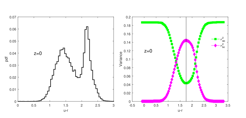
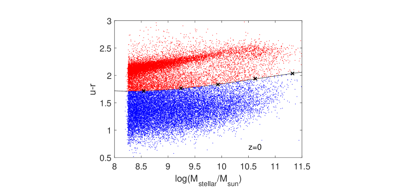
Figure 1: The top left panel shows the ($u-r$) colour distribution of galaxies. The top right panel shows the within-class variance $\sigma^{2}_{wc}$ and between-class variance $\sigma^{2}_{bc}$ of the entire sample as function of $u-r$ color. The vertical black line shows the ($u-r$) colour threshold for separating the red and blue galaxies. The bottom panel shows the red (red dots) and blue galaxies (blue dots) in the colour-stellar mass plane. The black crosses represent the threshold colour obtained in different stellar mass bins. The solid black line is obtained by fitting a cubic polynomial to the threshold values. The results shown here are for redshift $z=0$.

3.1 Classifying the red and blue galaxies

We classify the galaxies as red and blue using a scheme based on the Otsu’s method [56]. Otsu’s technique [62] was initially proposed to separate the foreground pixels from the background pixels in a grayscale image based on their intensities. The pixels with intensities greater than a threshold value are marked as foreground. The remaining pixels with intensities less than or equal to the threshold are labelled as background. This method is most suitable for a bimodal distribution of pixel intensities. It converts the input grayscale image into a binary image with foreground and background pixels.

The $(u-r)$ colour distribution of galaxies shows a bimodal nature with two distinct peaks [63, 64, 65]. The bimodality in colour is also evident for the galaxies in the EAGLE simulation (Figure 1). The classification scheme used in this work is ideal for any such distribution. We apply this technique to the $(u-r)$ colour distribution of the galaxies from the EAGLE simulation at $z=0$. We first calculate the histogram of $(u-r)$ colour of galaxies with $M$ number of bins. [56] show that the classification scheme is independent of the choice of number of bins. We choose $M=100$ for the present analysis. We then normalize the histogram by dividing the number of galaxies in each bin by the total number of galaxies N. The probability of galaxies $p_{i}$ associated with the $i^{th}$ bin is then given by $p_{i}=\frac{n_{i}}{N}$. Here $n_{i}$ represents the number of galaxies in the $i^{th}$ bin. The resulting probability distribution of galaxies is then used to calculate the probabilities of class occurrence for the red sequence and the blue cloud. If $k^{th}$ bin in the histogram corresponds to the threshold, then bins $[1,....,k]$ belong to the blue cloud and $[k+1,....,M]$ belong to the red sequence. If $B$ and $R$ respectively denote blue cloud and red sequence, the probability of class occurrence for the two populations are respectively given by,

$$P_{B}=\sum^{k}_{i=1}p_{i}$$ (3.1)

$$P_{R}=\sum^{M}_{i=k+1}p_{i}$$ (3.2)

The class means for each threshold for the two class $B$ and $R$ are given by,

$$\mu_{B}=\frac{\sum^{k}_{i=1}c_{i}p_{i}}{P_{B}}$$ (3.3)

$$\mu_{R}=\frac{\sum^{M}_{i=k+1}c_{i}p_{i}}{P_{R}}$$ (3.4)

Here $c_{i}$ represents the mean $(u-r)$ colour corresponding to the $i^{th}$ bin. The class variances for $B$ and $R$ are then respectively given by,

$$\sigma^{2}_{B}=\frac{\sum^{k}_{i=1}(c_{i}-\mu_{B})^{2}p_{i}}{P_{B}}$$ (3.5)

$$\sigma^{2}_{R}=\frac{\sum^{M}_{i=k+1}(c_{i}-\mu_{R})^{2}p_{i}}{P_{R}}$$ (3.6)

The within-class variance $\sigma^{2}_{wc}$ and between-class variance $\sigma^{2}_{bc}$ can be respectively written as,

$$\sigma^{2}_{wc}=P_{B}\sigma^{2}_{B}+P_{R}\sigma^{2}_{R}$$ (3.7)

$$\sigma^{2}_{bc}=P_{B}P_{R}(\mu_{B}-\mu_{R})^{2}$$ (3.8)

Otsu’s method iteratively searches for the threshold that minimizes the within-class variance or maximizes the between-class variance. We show the within-class variance (Equation 3.7) and between-class variance (Equation 3.8) of the entire sample as a function of $(u-r)$ colour threshold in the right panel of Figure 1. It is clearly seen that $\sigma^{2}_{wc}$ is minimum and $\sigma^{2}_{bc}$ is maximum at the same $(u-r)$ colour threshold. We consider this optimum $(u-r)$ colour threshold for separating the galaxies into the “blue cloud” and the “red sequence”. We classify the galaxies with a colour greater than the threshold as red. Similarly, galaxies whose colour is less than the threshold are classified as blue. It is well known that the galaxy colour depends on the stellar mass. The stellar mass of the galaxies varies over a wide range, and one can not apply a single colour threshold to divide the galaxies into the red and blue populations. We segregate the galaxies according to their stellar mass into different mass bins. We then apply the same technique to the galaxies in different mass bins. It provides a separate $(u-r)$ colour threshold for each mass bin. The colour threshold obtained as a function of the stellar mass is shown in the bottom panel of Figure 1. We find that the colour threshold increases with increasing stellar mass. We fit the threshold values as a function of the stellar mass with a smooth cubic polynomial as shown in Figure 1. The classified galaxies and the line separating them are shown in the colour-stellar mass plane in Figure 1. The results shown in Figure 1 correspond to the galaxies in the simulation at $z=0$. We apply the same technique to the simulation outputs at different redshifts and classify the red and blue galaxies analogously.

3.2 Local environment

We calculate the local density $(\eta_{k})$ at the location of each galaxies using the $k^{th}$ nearest neighbour method [55]. The local density $\eta_{k}$ given by,

$$\eta_{k}=\frac{k-1}{\frac{4}{3}\pi r^{3}_{k}}$$ (3.9)

Here $r_{k}$ is the distance from the galaxy to its $k^{th}$ nearest neighbour. We consider the distance to the $5^{th}$ nearest neighbour by taking $k=5$ in this analysis.

3.3 Clustering strength

We quantify the clustering strength of the galaxies in our sample using the two point correlation function $\xi(r)$. The two point correlation function $\xi(r)$ traces the amplitude of clustering strength as function of length scale $r$. $\xi(r)$ is a measure of the excess probability of finding two galaxies at a given separation $r$ compared to an unclustered random Poisson distribution. We use the Peebles & Hauser estimator [66] for measuring $\xi(r)$. The $\xi(r)$ is given by,

$$\xi(r)=\frac{DD(r)}{RR(r)}-1$$ (3.10)

Here $DD(r)$ and $RR(r)$ respectively represents the number of galaxy pairs in data and random Poisson distribution for separation $r$.

It is well known that $\xi(r)$ for galaxies exhibit a power law behaviour [67] ,

$$\xi(r)=\left(\frac{r}{r_{o}}\right)^{-\gamma}$$ (3.11)

where $r_{0}$ represents the correlation length.

3.4 Identifying galaxy pairs and building control samples of isolated galaxies

We identify the galaxy pairs in the EAGLE simulation following the strategy described in Das et al. (2023) [68]. We consider a galaxy and its first nearest neighbour as a pair if their separation in real space $r\leq 200$ kpc. Here, $r$ refers to the three-dimensional separation between the locations of their minimum gravitational potential. We identify the paired galaxies at redshift $z=0,0.5,1,1.49,2.01,2.48,3.02$. We also prepare control samples of isolated galaxies for the identified pairs at redshift $z=0,1,2.01,3.02$. We identify the isolated galaxies in the simulation volume as those that do not have a neighbour within a radius of 1 Mpc around them. We prepare a control sample of isolated galaxies by matching their stellar mass and local density with the paired galaxies. The isolated galaxies are matched to the paired galaxies within $\Delta_{mass}$ =0.08 dex and $\Delta_{\eta_{5}}=0.006$ $Mpc^{-3}$. We compare the distributions of stellar mass and the local density of the pair and control-matched sample by applying Kolmogorov-Smirnov (KS) test. The values of $\Delta_{mass},$ $\Delta_{\eta_{5}}$ are chosen in such a way that the null hypothesis for the distributions of stellar mass, local density of the pair and the control sample can be rejected at $\leq 40\%$ confidence level. It ensures that the distributions of stellar mass and local density of the paired and isolated galaxies are highly likely to be drawn from the same parent population.

The galaxy pairs are identified based on the three-dimensional physical separation between the galaxies in real space. Some of the identified pairs may belong to the galaxy groups or clusters. To avoid these pairs, we also impose an additional condition that the pair members must have their second nearest neighbour at a distance $>500$ kpc. We repeat our pair search and identify the set of galaxy pairs from the different snapshots between $z=0-3$. At each redshift, the control samples of these paired galaxies are also prepared from the samples of the isolated galaxies by matching their stellar mass and environment.

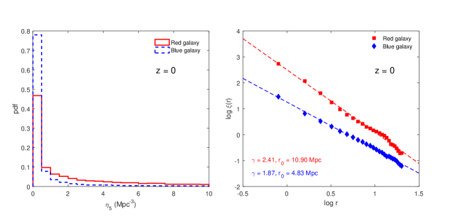
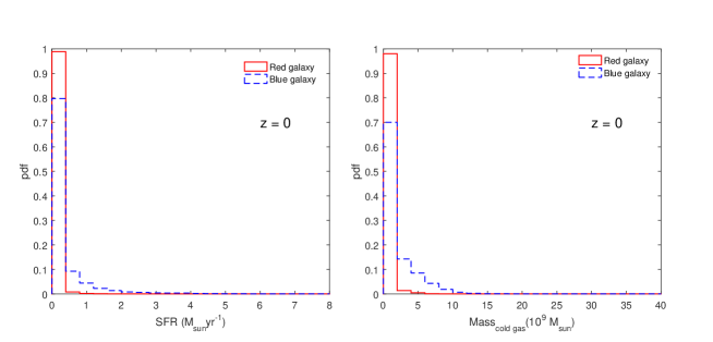
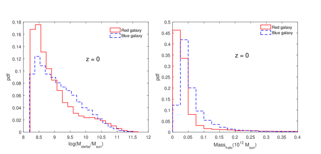
Figure 2: The top left panel compares the PDFs of the local density of the red and blue galaxies at redshift $z=0$. The two-point correlation functions of the red and blue galaxies at the same redshift are compared in the top right panel. The best fit lines to the correlation functions and the fitted parameters are shown together in the same panel. The middle left, middle right, bottom left and the bottom right panels respectively compare the distributions (PDFs) of the SFR, cold gas mass, stellar mass and halo mass of the red and blue galaxies at $z=0$.

Figure 3: The different panels compares the PDFs of the local density of the red and blue galaxies at different redshifts between $z=0.5-3.02$.

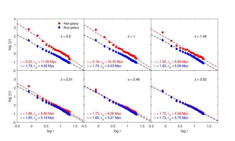
Figure 4: The different panels compare the two-point correlation function of the red and blue galaxies at different redshifts between $z=0.5-3.02$. The best fit lines and the associated parameters are shown together in each panel.

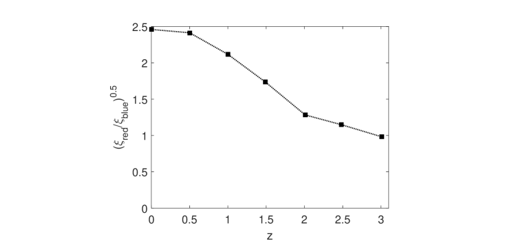
Figure 5: This shows the relative bias of the red and blue galaxies as a function of redshift between $z=3.02-0$.

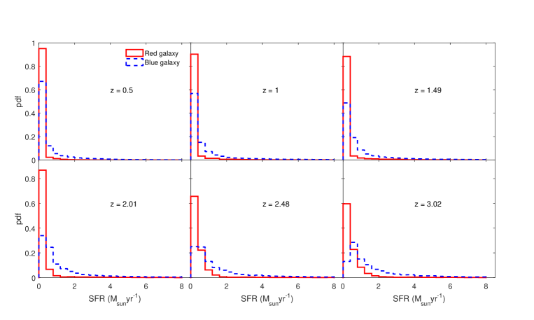
Figure 6: Same as Figure 3, but for SFR.

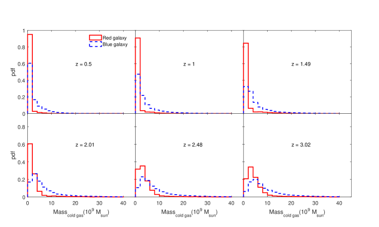
Figure 7: Same as Figure 3, but for cold gas mass.

4 Results

We first compare the local density, clustering strength, SFR, cold gas mass, stellar mass and the dark matter halo mass of the red and blue galaxies at the present epoch. The results are shown in different panels of Figure 2.

The top left panel of Figure 2 compares the PDF of the local density of the red and blue galaxies in the present universe. It clearly shows that the blue galaxies primarily reside in the low-density environments, whereas the red galaxies dominate the high-density environments. A comparison of the two-point correlation function of the red and blue galaxies in the top right panel of Figure 2 shows that the red galaxies are strongly clustered compared to the blue galaxies. On average, the clustering strength of the red galaxies is $\sim 6$ times stronger compared to the blue galaxies within $r<20$ Mpc. Also, the correlation length ($r_{0}$) of the red galaxies is more than twice that of the blue galaxies. The galaxies residing in the high-density regions are expected to be more strongly clustered. The fact that the red galaxies are preferentially located in the high-density environment is consistent with their stronger clustering strength. The middle left and right panels of Figure 2 compare the SFR and cold gas mass distributions of the red and blue galaxies at $z=0$. These show that, in general, the galaxies in the present universe have a low cold gas mass reservoir. Notably, the red galaxies have nearly depleted their entire cold gas mass reservoir, resulting in negligible or no star formation. It would also be interesting to compare the stellar and halo mass distributions of the red and blue galaxies at present. The bottom left panel of Figure 2 compares the PDF of the stellar mass distributions of the red and blue galaxies at $z=0$. Interestingly, the red population dominates the blue population both at the low and the high end of the stellar mass distributions. The red galaxies at the low stellar mass end could be the quenched satellite galaxies, whereas those at the high stellar mass end could be the massive central galaxies that have quenched their star formation through mass quenching or AGN feedback. We find an analogous behaviour in the halo mass distribution of the red galaxies as shown in the bottom right panel of Figure 2. A large fraction of the galaxies in the red population are hosted in the smaller mass halos. These smaller mass halos may correspond to the low-mass satellite galaxies.

We now study the evolution of the properties of the red and blue galaxies as a function of redshift. We compare the PDF of the local density of the red and blue galaxies at different redshifts in the different panels of Figure 3. The results show that the local environment of the red and blue galaxies have smaller differences up to $z=2.01$. The differences in their local environment increase progressively with decreasing redshift. The number of blue galaxies dominates the low-density environment, whereas the red galaxies progressively dominate the high-density environments. A comparison of the two-point correlation function of the red and blue galaxies across different redshifts in Figure 4 confirm the same trend. It shows that the red and blue galaxies have similar clustering strength up to $z=2.48$. The red galaxies cluster more strongly than the blue galaxies after $z=2.01$. The differences in the values of $\gamma$ and $r_{0}$ for the red and blue galaxies increase with time. We show the relative bias between the red and blue galaxies as a function of redshift in Figure 5. Figure 5 shows that the red and blue galaxies have the same bias at $z\sim 3$. The relative bias proliferates after $z=2$, reaching a value of $2.5$ at $z=0$. These results indicate that the environment may not entirely decide the transformation of galaxy colour before $z=2$. The environmental factors dominate at smaller redshifts ($z<2$), leading to significant evolution in galaxy properties.

We compare the SFR distributions of the red and blue galaxies at different redshifts in Figure 6. The distributions of the cold gas mass in these two populations are compared at different redshifts in Figure 7. Both Figure 6 and Figure 7 confirm a strong correlation between the SFR and the cold gas mass in both the red and blue galaxies. Interestingly, the SFR and cold gas mass distributions of the red and blue galaxies are significantly different between $2\leq z\leq 3$ even though their local environment and the clustering strength have smaller differences during this period (Figure 3 and Figure 4). It implies that the dichotomy in the star formation histories of galaxies does not originate only from the differences in their local density. The size of the cold gas mass reservoir in galaxies may be related to the gas accretion efficiency of their host dark matter halos. The greater abundance of the cold gas mass in some galaxies may lead to higher SFR. At lower redshifts $z<2$, the environmental factors like starbursts during galaxy interactions [25, 26, 27, 28, 29] boost the conversion efficiency of gas to stars, eventually depleting their cold gas reservoir. Several other environment-driven physical mechanisms such as ram pressure stripping [21], harassment [38], starvation [40] and feedback from supernovae and AGN [22, 23] can prevent the gas replenishment or expel the gas from the galaxy, eventually quenching the star formation.

The galaxy interactions play an important role in the evolution of the galaxy properties. The interactions may significantly impact the colour of a galaxy and its evolution. We compare the cumulative median SFR of the paired galaxies as a function of the pair separation at different redshifts in the top left panel of Figure 8. The paired galaxies have a higher median SFR at a given pair separation in the past. It increases with the redshift, implying that the tidal interactions are more efficient in triggering starburst in the paired galaxies at higher redshifts ($z>0.5$). An anomalous behaviour is observed at $z=2.01$ where the paired galaxies with separation $<50$ kpc exhibit a higher median SFR than those with the same separation at $z=2.48$. It indicates a surge in close galaxy interactions around $z\sim 2$, which significantly enhanced tidally triggered star formation. It is consistent with the results shown in Figure 3, Figure 4 and Figure 5. The environmental factors dominate after redshift $2$ due to significant evolution in the local density and clustering. The enhancement in the local density and clustering increases the probability of interaction between galaxies. The SFR is strongly enhanced when two gas-rich galaxies interact with each other. The starburst activity consumes the available gas in a galaxy, gradually depleting its cold gas reservoir. The median SFR is reduced at all pair separations with decreasing redshift after $z=1.49$. The gradual depletion of the cold gas reservoir causes a reduction in the median SFR with decreasing redshift.

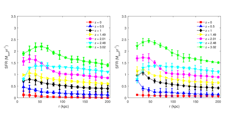
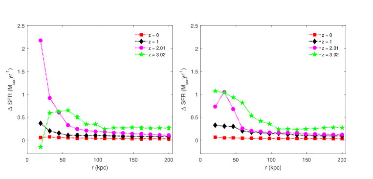
Figure 8: The top left panel shows the cumulative median SFR of the paired galaxies as a function of the pair separation at different redshifts between $z=3.02-0$. The difference between the cumulative median SFR of the paired galaxies and the control-matched isolated galaxies is shown as a function of the pair separation at different redshifts in the bottom left panel. The top right and bottom right panels show the same but for the paired galaxies, which have their second nearest neighbour at a distance $>500$ kpc. The 1$\sigma$ errors shown at each data point are obtained from $10$ Jackknife samples drawn from the original data.

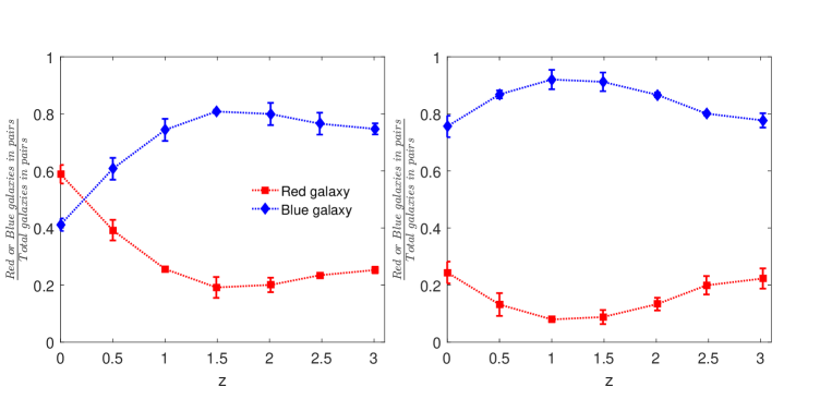
Figure 9: The left panel shows the ratio of the red or blue galaxies in pairs to the total galaxies in pairs at different redshifts. The right panel shows the same but only considering the paired galaxies with their second nearest neighbour at a distance $>500$ kpc. The 1$\sigma$ errors shown here are obtained from $10$ Jackknife samples drawn from the original data.

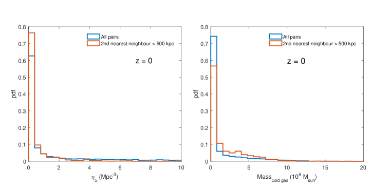
Figure 10: The left panel of this figure compares the local density distribution of all galaxy pairs with the pairs having their second nearest neighbour at a distance $>500$ kpc. The right panel compares the cold gas mass distribution for the same pairs.

We calculate the difference between the cumulative median SFR of the paired galaxies and the control-matched isolated galaxies at each pair separation. We show the results in the bottom left panel of Figure 8. The results are shown for $4$ different redshifts. The SFR enhancement in galaxy pairs can be seen in this figure. The impact of the tidally triggered SFR enhancement decreases with the increasing pair separation. Also, $\Delta SFR$ decreases at each pair separation, with the decreasing redshift confirming the trends observed in the top left panel.

We repeat our analysis for the galaxy pairs for which the member galaxies do not have their second nearest neighbour within $500$ kpc. The results are shown in the top right and bottom right panels of Figure 8. We observe a very similar trend in these panels. However, the SFR enhancement at smaller pair separation is more pronounced for these pairs. Interestingly, the SFR enhancement at $z=2.01$ is less pronounced at smaller pair separation for these pairs (bottom right panel of Figure 8). Most of these isolated pairs do not belong to the denser regions like groups and clusters where a higher frequency of close interactions at $z\sim 2$ elevate the SFR to a great extent.

It would also be interesting to study the fraction of red or blue galaxies in paired systems as a function of redshift. We show the fraction of red and blue galaxies that are members of galaxy pairs having a separation of $<200$ kpc in the left panel of Figure 9. We find that a large fraction ($\sim 75\%$) of interacting galaxies are blue at $z\sim 3$. The fraction of blue galaxies slowly increases upto $z=1.5$, after which it steadily declines to $\sim 40\%$ at $z=0$. The fraction of red galaxies rises from $\sim 20\%$ at $z=1.5$ to $\sim 60\%$ at $z=0$, indicating a decline in the efficiency of tidally induced SFR due to the gradual exhaustion of the cold gas supply in galaxies. Both galaxy interactions and environmental effects may have a role in it. The fraction of red and blue galaxies becomes nearly equal around a redshift of $z=0.25$. This transition could be sensitive to the background cosmology and the details of the galaxy formation and evolution. We propose that such a transition may be used as a possible diagnostic of the different cosmological parameters and the parameters of the galaxy formation models. We now shift our attention to the isolated pairs for which the second nearest neighbour must lie beyond a distance of $500$ kpc. We show the fraction of red and blue galaxies in such pairs as a function of redshift in the right panel of Figure 9. The fraction of blue galaxies in these pairs rises slowly from $\sim 80\%$ at $z=3$ to $\sim 90\%$ at $z=1$ and then decreases mildly to $\sim 75\%$ at $z=0$. A smaller fraction ($\sim 25\%$) of red galaxies in isolated pairs at $z=0$ indicates that the isolated pairs are less affected by the environmental factors. In the left panel of Figure 10, we compare the local density distributions of all pairs with the pairs having their second nearest neighbour beyond $500$ kpc. The pairs with their second nearest neighbour at a distance $>500$ kpc reside in the less dense environments. The right panel of Figure 10 shows that these pairs have a relatively larger cold gas reservoir. A larger cold gas supply would delay the quenching in such galaxy pairs. The differences in the size of the gas reservoirs may arise due to their different evolutionary history.

5 Conclusions

We classify the red and blue galaxies in the EAGLE simulation at different redshifts and study the evolution of their environment, clustering and physical properties as a function of redshift. We also study the cumulative median SFR and the SFR enhancement in interacting galaxies as a function of the pair separation at different redshifts. These together allow us to study the combined roles of environment and galaxy interactions in the evolution of galaxies. Our primary results are as follows:

(i) In the present universe, the red galaxies preferentially reside in the denser environments, whereas the blue galaxies inhabit the lower-density regions. The red galaxies are more strongly clustered than the blue galaxies. The blue galaxies have a larger cold gas mass and higher SFR than the red galaxies. The red galaxies dominate the blue galaxies at the lower and higher ends of the stellar mass distribution. The lower and higher stellar mass populations in the red sequence could be the quenched satellites and the massive central galaxies, respectively.

(ii) The differences in the local density and the clustering strength of the red and blue galaxies rise strongly with the decreasing redshift after $z=2$. The relative bias between the red and the blue galaxies increases from $1$ to $2.5$ between $z=3-0$. The asymmetry in the cold gas mass and SFR distributions of the red and blue galaxies are amplified by the environmental factors after $z=2$.

(iii) The dichotomy between the star formation history of the galaxies exists at all redshifts between $z=0-3$. The cold gas mass and the SFR distributions of the red and blue galaxies differ significantly between $z=3-2$ even though the differences in environments and clustering strengths are relatively smaller during this period. It indicates that the dichotomy between the two populations does not arise due to the environment alone. Such differences may be related to the assembly history and the gas accretion efficiency of their host dark matter halos.

(iv) Interacting galaxy pairs at a given separation have a larger median SFR at higher redshifts. The median SFR at all separations reduce with the decreasing redshift, implying a gradual exhaustion of the cold gas supply in interacting galaxies. An anomalous increase in the median SFR at smaller pair separation is observed around $z\sim 2$. It indicates that environmental factors start to dominate around this redshift, increasing the frequency of interactions and leading to starbursts in many close pairs.

(v) The median SFR of the interacting pairs are elevated compared to the mass-matched and environment-matched isolated galaxies at nearly all pair separations within $r<200$ kpc. The degree of enhancement declines at lower redshifts. It implies that the interaction-induced star formation is more efficient at higher redshifts due to the availability of large amounts of cold gas in galaxies.

(vi) The fraction of blue galaxies in interacting pairs increases with the decreasing redshift upto $z=1.5$. It steeply declines after this redshift until the present. It may arise due to the depletion of cold gas supply in the interacting galaxies due to starbursts and other environmental effects. The blue fraction does not decline strongly in pairs that have their second nearest neighbour at a distance $>500$ kpc. Only a mild decrease in the blue fraction is observed in such pairs. These galaxy pairs reside in low-density environments where the environmental factors less impact them. They have a larger cold gas supply, which enables them to delay the quenching.

We compare our results with the other studies with the EAGLE and Illustris TNG simulations [69]. [58] study the evolution of galaxy colour using the EAGLE simulation. They find that the red sequence builds up at $z\sim 1$ due to the quenching of low-mass satellite galaxies and AGN feedback in the more massive central galaxies. [59] show that the quenching time scales for both the central and satellite galaxies in the EAGLE simulation decrease with the increasing stellar mass. They find a growth in the fraction of passive galaxies at lower redshifts. Using TNG100 and TNG300, [60] show that $70\%-90\%$ of centrals and satellites with mass $\geq 10^{10}M_{\odot}$ are predicted to be quenched between $0\leq z\leq 0.5$. Another study [61] with the TNG simulation finds that the slow-quenching galaxies are about twice as common as the fast-quenching galaxies in the redshift range $0.7<z<2$. Our results are consistent with these findings.

Our results are also consistent with the observational findings [48, 45, 46, 47] indicating that the hydrodynamical simulations are a powerful tool for studying galaxy formation and evolution. A recent study [70] with the photometric data from the S-PLUS DR4 survey find a high fraction of red galaxies in paired systems. They show that the red pair fractions increase in closer pairs and pairs of similar luminosity, indicating that shared environments and interactions have important roles in the evolution of galaxy colour. Our analysis with the EAGLE simulation also indicates that both interactions and environment play crucial roles in the galaxy evolution. However, the dichotomy between the red and blue galaxies may not arise due to the environment alone. The differences in the evolutionary history may lead to galaxies with different cold gas content and star formation rates. The environment and interactions at lower redshifts amplify these differences, splitting the galaxies into two distinct populations.

References

- [1] I. Strateva, et al., AJ, 122, 1861 (2001)
- [2] M. R. Blanton, et al., ApJ, 594, 186 (2003)
- [3] E. F. Bell, D. H. McIntosh, N. Katz, M. D. Weinberg, ApJS, 149, 289 (2003)
- [4] M. L Balogh, I. K. Baldry, R. Nichol, C. Miller, R. Bower, K. Glazebrook, 2004, ApJL, 615, L101 (2004)
- [5] I. K. Baldry, K. Glazebrook, J. Brinkmann, Ž. Ivezić, R. H. Lupton, R. C. Nichol, A. S. Szalay, ApJ, 600, 681 (2004)
- [6] P. B. Tissera, R. Domínguez-Tenreiro, C., Sáiz A. Scannapieco, MNRAS, 333, 327 (2002)
- [7] D. W. Hogg, et al., ApJ Letters, 601, L29 (2004)
- [8] I. K. Baldry, M. L. Balogh, R. Bower, K. Glazebrook, R. C. Nichol, AIP Conference Proceedings, 743, 106 (2004)
- [9] M. R. Blanton, D. Eisenstein, D. W. Hogg, D. J. Schlegel, J. Brinkmann, ApJ, 629, 143 (2005)
- [10] C. Park, et al. 2005, ApJ, 633, 11 (2005)
- [11] B. Pandey, & S. Bharadwaj, MNRAS, 357, 1068 (2005)
- [12] I. Zehavi, et al., ApJ, 630, 1 (2005)
- [13] B. Pandey, & S. Bharadwaj, MNRAS, 372, 827 (2006)
- [14] N. M. Ball, J. Loveday, R. J. Brunner, MNRAS, 383, 907 (2008)
- [15] S. P. Bamford, R. C. Nichol, I. K. Baldry, et al., MNRAS, 393, 1324 (2009)
- [16] M. C. Cooper, A. Gallazzi, J. A. Newman, R. Yan, MNRAS, 402, 1942 (2010)
- [17] B. Pandey, S. Sarkar, MNRAS, 498, 6069 (2020)
- [18] A. Nandi, B. Pandey, P. Sarkar, 2023, Accepted in JCAP, arXiv:2306.05354 (2023)
- [19] A. Dekel, Y. Birnboim, MNRAS, 368, 2 (2006)
- [20] A. H. Maller, J. S. Bullock, MNRAS, 355, 694 (2004)
- [21] J. E. Gunn, & J. R. Gott, ApJ, 176, 1 (1972)
- [22] T. J. Cox, J. Primack, P. Jonsson, & R. S. Somerville, ApJL, 607, L87 (2004)
- [23] N. Murray, E. Quataert, & T. A. Thompson, ApJ, 618, 569 (2005)
- [24] V. Springel, T. Di Matteo, & L. Hernquist, MNRAS, 361, 776 (2005)
- [25] E. J. Barton, M. J. Geller, S. J. Kenyon, ApJ, 530, 660 (2000)
- [26] D. G. Lambas, P. B. Tissera, M. S. Alonso, G. Coldwell, MNRAS, 346, 1189 (2008)
- [27] M. S. Alonso, P. B. Tissera, G. Coldwell, D. G. Lambas, MNRAS, 352, 1081 (2004)
- [28] B. Nikolic, H. Cullen, P. Alexander, MNRAS, 355, 874 (2004)
- [29] D. F. Woods, M. J. Geller, E. J. Barton, AJ, 132, 197 (2006)
- [30] D. F. Woods, M. J. Geller, AJ, 134, 527 (2007)
- [31] E. J. Barton, J. A. Arnold, A. R. Zentner, J. S. Bullock, R. H. Wechsler, ApJ, 671, 1538 (2007)
- [32] S. L. Ellison, D. R. Patton, L. Simard, A. W. McConnachie, AJ, 135, 1877 (2008)
- [33] S. L. Ellison, D. R. Patton, L. Simard, A. W. McConnachie, I. K. Baldry, J. T. Mendel, MNRAS, 407, 1514 (2010)
- [34] D. F. Woods, M. J. Geller, M. J. Kurtz, E. Westra, D. G. Fabricant, I. Dell’Antonio, AJ, 139, 1857 (2010)
- [35] D. R. Patton, S. L. Ellison, L. Simard, A. W. McConnachie, J. T. Mendel, MNRAS, 412, 591 (2011)
- [36] A. Das, B. Pandey, S. Sarkar S., RAA, 23, 025016 (2022)
- [37] M. L. Balogh, J. F. Navarro,, & S. L. Morris, ApJ, 540, 113 (2000)
- [38] B. Moore, N. Katz, G. Lake, A. Dressler, & A. Oemler, A., Nature, 379, 613 (1996)
- [39] B. Moore, G. Lake, & N. Katz, N., ApJ, 495, 139 (1998)
- [40] R. B. Larson, B. M. Tinsley,, & C. N. Caldwell, ApJ, 237, 692 (1980)
- [41] R. S. Somerville, & J. R. Primack, MNRAS, 310, 1087 (1999)
- [42] D. Kawata & J. S. Mulchaey, ApJL, 672, L103 (2008)
- [43] M. Martig, F. Bournaud, R. Teyssier, A. Dekel, ApJ, 707, 250 (2009)
- [44] K. L. Masters, M. Mosleh, A. K. Romer, R. C. Nichol, S. P. Bamford, K. Schawinski, C. J. Lintott, et al., MNRAS, 405, 783 (2010)
- [45] K.-V. H. Tran, C. Papovich, A. Saintonge, M. Brodwin, J. S. Dunlop, D. Farrah, K. D. Finkelstein, et al., ApJL, 719, L126 (2010)
- [46] N. M. Förster Schreiber, S. Wuyts, ARA&A, 58, 661 (2020)
- [47] A. Gupta, K.-V. Tran, J. Cohn, L. Y. Alcorn, T. Yuan, V. Rodriguez-Gomez, A. Harshan, et al., ApJ, 893, 23 (2020)
- [48] P. Madau, H. C. Ferguson, M. E. Dickinson, M. Giavalisco, C. C. Steidel, & A. Fruchter, MNRAS, 283, 1388 (1996)
- [49] Schaye J. et al. (The EAGLE project), MNRAS, 446, 521 (2015)
- [50] McAlpine S., Helly J. C., Schaller M., Trayford J. W. et al., A&A , 72, 15 (2016)
- [51] Crain R A., et al., MNRAS, 450, 1937 (2015)
- [52] Planck Collaboration et al., A&A, 571, A1 (2014)
- [53] Doi M., et al., doi:10.1088/004-6256/139/4/1628, arxiv:1002.3701, 2010
- [54] Trayford J W et al., MNRAS, 452, 2879 (2015)
- [55] Casertano Hut. & Hut P., ApJ, 298, 80 (1985)
- [56] Pandey B., Astronomy and Computing, 44, 100725 (2023)
- [57] M. Furlong, R. G. Bower, T. Theuns, J. Schaye, R. A. Crain, M. Schaller, C. Dalla Vecchia, et al., MNRAS, 450, 4486 (2015)
- [58] J. W. Trayford, T. Theuns, R. G. Bower, R. A. Crain, C. del P. Lagos, M. Schaller, J. Schaye, MNRAS, 460, 3925 (2016)
- [59] R. J. Wright, C. del P. Lagos, L. J. M. Davies, C. Power, J. W. Trayford, O. I. Wong, MNRAS, 487, 3740 (2019)
- [60] M. Donnari, A. Pillepich, G. D. Joshi, D. Nelson, S. Genel, F. Marinacci, V. Rodriguez-Gomez, et al., MNRAS, MNRAS, 500, 4004 (2021)
- [61] D. Walters, J. Woo, S. L. Ellison, MNRAS, 511, 6126 (2022)
- [62] Otsu N., IEEE Trans. Syst. Man Cybern., 9, 62 (1979)
- [63] Strateva I. et al., AnJ, 122, 1861 (2001)
- [64] Balogh M, L., Baldry I, K., Nichol R., Miller C., Bower R., Glazebrook K., ApJL, 615, L101
- [65] Baldry I, K., Glazebrook K., Brinkmann J., Lupton R, H. et al., ApJ, 600, 681 (2004)
- [66] Peebles P J E. & Hauser M G., ApJS, 19, 28 (1974)
- [67] Peebles P J E. & Groth E J., ApJ, 196, 1 (1975)
- [68] Das A., Pandey B. & Sarkar S., RAA, 11, 23 (2023)
- [69] D. Nelson, V. Springel, A. Pillepich, V. Rodriguez-Gomez, P. Torrey, S. Genel, M. Vogelsberger, et al., 2019, Computational Astrophysics and Cosmology, 6, 2 (2019)
- [70] M. C. Cerdosino, A. L. O’Mill, F. Rodriguez, A. Taverna, Jr L. Sodré, E. Telles, H. Méndez-Hernández, et al., Accepted in MNRAS, arXiv:2402.00120 (2024)