How do Transformers perform
In-Context Autoregressive Learning?

Abstract

Transformers have achieved state-of-the-art performance in language modeling tasks. However, the reasons behind their tremendous success are still unclear. In this paper, towards a better understanding, we train a Transformer model on a simple next token prediction task, where sequences are generated as a first-order autoregressive process $s_{t+1}=Ws_{t}$. We show how a trained Transformer predicts the next token by first learning $W$ in-context, then applying a prediction mapping. We call the resulting procedure in-context autoregressive learning. More precisely, focusing on commuting orthogonal matrices $W$, we first show that a trained one-layer linear Transformer implements one step of gradient descent for the minimization of an inner objective function, when considering augmented tokens. When the tokens are not augmented, we characterize the global minima of a one-layer diagonal linear multi-head Transformer. Importantly, we exhibit orthogonality between heads and show that positional encoding captures trigonometric relations in the data. On the experimental side, we consider the general case of non-commuting orthogonal matrices and generalize our theoretical findings.

1 Introduction

Transformers (Vaswani et al., 2017) have achieved state-of-the-art performance in natural language processing tasks (Devlin et al., 2018). They now serve as the backbone for large language models, such as GPT (Radford et al., 2018; Brown et al., 2020), Chinchilla (Hoffmann et al., 2022), PaLM (Chowdhery et al., 2023), LLama (Touvron et al., 2023) or Mistral (Jiang et al., 2023). These models, which are causal in nature, are trained to predict the next token $s_{T+1}$ given a sequence (also termed as context) $s_{1:T}\coloneqq(s_{1},\cdots,s_{T})$. An intriguing property of large Transformers is their ability to adapt their computations given the context $s_{1:T}$. In this work, we make a step towards understanding this in-context learning ability. More precisely, assuming the tokens satisfy a relation $s_{T+1}=\varphi_{W}(s_{1:T})$, with $W$ a context-dependent parameter varying with each sequence, we say that a trained Transformer autoregressively learn this relation in-context if it decomposes its prediction into 2 steps: first, estimating $W$ through an in-context mapping, and then applying a simple prediction mapping, which is equal or closely related to $\varphi_{W}$ (see Definition 1).

The goal of this paper is to explore a simple form of $\varphi_{W}$ and to characterize, as precisely as possible, the in-context and prediction mappings for optimally-trained Transformers. Building on the work of Von Oswald et al. (2023b), we focus on a simple autoregressive (AR) process of order $1$, where each sequence is generated following the recursion $s_{T+1}=\varphi_{W}(s_{1:T})\coloneqq Ws_{T}$ , and $W$ is a randomly sampled orthogonal matrix, referred to as the context matrix. Such a process is illustrated in dimension $3$ in Figure 1 for two different matrices $W$. We investigate the training of a linear Transformer to predict the next token in these AR processes, examining how it estimates $W$ in-context and makes predictions for $s_{T+1}$. Depending on the input tokens encoding, the in-context mapping can correspond to gradient descent on an inner objective, as suggested by Von Oswald et al. (2023b). Alternatively, the context matrix $W$ might be determined in closed form if the model possesses sufficient expressiveness. This paper investigates both scenarios.

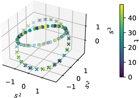
Figure 1: Illustration of the autoregressive process in $\mathbb{R}^{3}$. Dots and crosses correspond to two different orthogonal matrices $W$.

More precisely, we make the following contributions:

• We begin by reviewing the background and related work in §2. Then, in §3, we introduce our autoregressive process, which allows us to mathematically formalize the notion of in-context autoregressive learning.

• In §4, we demonstrate that if the matrices $W$ commute and the model parameters possess a block structure, then a linear Transformer—trained on augmented tokens as introduced by Von Oswald et al. (2023b)—effectively implements a step of gradient descent on an underlying objective function as in-context mapping.

• In §5, we turn our attention to a one-layer linear attention Transformer that incorporates positional encoding but does not use augmented tokens. We comprehensively characterize the minimizers of the training loss. Notably, these minimizers display an orthogonality property across different heads. This aspect underscores the significance of positional encoding in enabling the Transformer to learn geometric operations between tokens through its in-context mapping. We also study positional-encoding-only attention, and show that approximate minimum $\ell_{2}$ norm solutions are favored by the optimization process.

• On the experimental side, in §6, we extend our analysis to the more general case where the context matrices $W$ do not commute. We validate our theoretical findings for both augmented and non-augmented scenarios. Furthermore, we explore how variations in the distribution of the context matrices $W$ affect trained positional encodings. We recover structures resembling the traditional positional encoding commonly used in Transformers.

Notations.

We use lower cases for vectors and upper cases for matrices. $\|.\|$ is the $\ell_{2}$ norm. We denote the transpose and adjoint operators by ^⊤ and ^⋆. $O(d)$ (resp $U(d)$) is the orthogonal (resp unitary) manifold, that is $O(d)=\{W\in\mathbb{R}^{d\times d}|W^{\top}W=I_{d}\}$ and $U(d)=\{W\in\mathbb{C}^{d\times d}|W^{\star}W=I_{d}\}$. The element-wise multiplication is $\odot$. $\langle|\rangle$ is the canonical dot product in $\mathbb{R}^{d}$, and $\langle|\rangle_{\mathbb{C}}$ the canonical hermitian product in $\mathbb{C}^{d}$. For $\lambda\in\mathbb{C}^{d}$, $\lambda^{k}$ is the element-wise power $k$ of $\lambda$: $(\lambda^{k})_{i}=\lambda^{k}_{i}$.

2 Background and previous works

Causal Language Modelling.

Language (or sequence) modeling refers to the development of models to predict the likelihood of observing a sequence $(x_{1},\dots,x_{T})$, where each $x_{t}$ is called a token, and comes from a finite vocabulary. This can be done by using the chain rule of probability $P(X_{1}=x_{1},X_{2}=x_{2},\ldots,X_{T}=x_{T})=P(X_{1}=x_{1})\times P(X_{2}=x_{2}|X_{1}=x_{1})\times\ldots\times P(X_{T}=x_{T}|X_{1}=x_{1},\ldots,X_{T-1}=x_{T-1})$ (Jurafsky & Martin, 2009). Predicting these conditional probabilities can be done using a parametrized model $\mathcal{F}_{\theta}$ to minimize the loss $L(\mathcal{F}_{\theta}(x_{1},...,x_{T-1}),x_{T})$ across all training samples and sequence length $T$. In common applications, $L$ is chosen as the cross-entropy loss. In other words, the model is trained to predict the next token sequentially. Such a model is called a causal language model: it cannot access future tokens. Recently, the Transformer has emerged as the model of choice for language modeling.

Transformers.

Transformers (Vaswani et al., 2017) process sequences of tokens $(x_{1},\dots,x_{T})$ of arbitrary length $T$. In its causal form (Brown et al., 2020; Touvron et al., 2023; Jiang et al., 2023), a Transformer first embeds the tokens to obtain a sequence $(e_{1},\dots,e_{T})$. It is then composed of a succession of blocks with residual connections (He et al., 2016). Each block is made of the composition of a multi-head self-attention module and a multi-layer perceptron. Importantly, the latter acts on each token separately, whereas multi-head self-attention mixes tokens, and corresponds to applying vanilla self-attention in parallel (Michel et al., 2019). More precisely, each multi-head self-attention is parametrized by a collection of weight matrices $(W^{h}_{Q},W^{h}_{K},W^{h}_{V},W^{h}_{O})_{1\leq h\leq H}$ and returns:

$$(\sum_{h=1}^{H}W^{h}_{O}\sum_{t^{\prime}=1}^{t}\mathcal{A}^{h}_{t,t^{\prime}}W^{h}_{V}e_{t^{\prime}})_{t\in\{1,\cdots,T\}},$$ (1)

where $\mathcal{A}^{h}$ is the attention matrix (Bahdanau et al., 2014) and is usually defined as

$$\mathcal{A}^{h}_{t,:}=\mathrm{softmax}(\langle W^{h}_{Q}e_{t},W^{h}_{K}e_{:}\rangle),$$

with $\langle\cdot,\cdot\rangle$ a dot product. The sum over $t^{\prime}$ in (1) stopping at $t$ reflects the causal aspect of the model: the future cannot influence the past. The output at position $T$ is commonly used to predict the next token $e_{T+1}$. In practice, to help the model encode the relative position of the tokens in the sequence, a positional encoding (PE) is used.

Positional encoding.

As described in Kazemnejad et al. (2023), encoding the position in Transformers amounts to defining the dot product $\langle,\rangle$ in the attention matrix, using additional (learnable or not) parameters. Popular designs include Absolute PE (Vaswani et al., 2017), Relative PE (Raffel et al., 2020), AliBI (Press et al., 2021), Rotay (Su et al., 2024), and NoPE (Kazemnejad et al., 2023). In this paper, we consider a learnable positional encoding.

Linear attention.

In its simplest form, linear attention (Katharopoulos et al., 2020) consists in replacing the $\mathrm{softmax}$ in (1) by the identity. More formally, it consists in considering that each coefficient in the attention matrix is $\mathcal{A}^{h}_{t,t^{\prime}}=\langle W^{h}_{K}e_{t^{\prime}},W^{h}_{Q}e_{t}\rangle$. The main practical motivation of linear attention is that it enables faster inference (Katharopoulos et al., 2020; Fournier et al., 2023). Note that even though they are called linear Transformers, the resulting models are non-linear with respect to the input sequence. From a theoretical perspective, linear attention has become the model of choice to understand the in-context-learning properties of Transformers (Mahankali et al., 2023; Ahn et al., 2023; Zhang et al., 2023).

In-context-Learning in Transformers

The seminal work of Brown et al. (2020) reported an in-context-learning phenomenon in Transformer language models: these models can solve few-shot learning problems given examples in-context. Namely, given a sequence $(x_{1},f(x_{1}),x_{2},f(x_{2}),\cdots,x_{n})$, a trained Transformer can infer the next output $f(x_{n})$ without additional parameter updates. This surprising ability has been the focus of recent research. Some works consider the $\mathrm{softmax}$ attention without considering training dynamics (Garg et al., 2022; Akyürek et al., 2022; Li et al., 2023). Other works focus solely on linear attention and characterize the minimizers of the training loss, when $f$ is sampled across linear forms on $\mathbb{R}^{d}$, that is $f(x)=w^{\top}x$ for some $w$ (Mahankali et al., 2023; Ahn et al., 2023; Zhang et al., 2023). In particular, these works discuss the ability of the Transformer to implement optimization algorithms in their forward pass at inference, as empirically suggested by Von Oswald et al. (2023a). Nevertheless, the formulations used by Von Oswald et al. (2023a); Mahankali et al. (2023); Ahn et al. (2023); Zhang et al. (2023) are all based on concatenating the tokens so that the Transformer’s input takes the form $\begin{pmatrix}x_{1}&x_{2}&\cdots&x_{n}\\ f(x_{1})&f(x_{2})&\cdots&0\end{pmatrix}\in\mathbb{R}^{(d+1)\times n}.$ However, the necessity for this concatenation limits the impact of these results as there is no guarantee that the Transformer would implement this operation in its first layer. In addition, these works explicitly consider the minimization of an in-context loss, which is different from the next-token prediction loss in causal Transformers. In contrast, our work considers the next-token prediction loss and considers a more general notion of in-context learning, namely in-context autoregressive learning, that we describe in the next section.

3 Linear Attention for AR Processes

Token encoding.

Building on the framework established by Von Oswald et al. (2023b), we consider a noiseless setting where each sequence begins with an initial token $s_{1}=1_{d}$. This token acts as a start-of-sentence marker. The subsequent states are generated according to $s_{t+1}=Ws_{t}$, where $W$ is a matrix referred to as the context matrix. This matrix is sampled uniformly from a subset $\mathcal{C}_{O}$ (respectively, $\mathcal{C}_{U}$) of $O(d)$ (respectively, $U(d)$), and we denote $\mathcal{W}$ as the corresponding distribution: $W\sim\mathcal{W}\coloneqq\mathcal{U}(\mathcal{C})$. Considering norm-preserving matrices ensures the stability of the AR process, which is crucial to be able to learn from long sequences (i.e. using large $T$). In this paper, we contrast $\mathcal{C}_{O}$ and $\mathcal{C}_{U}$ to showcase how the distribution of in-context parameters $W$ impacts the in context mapping learned by Transformers. It is also worth noting that $U(d)$ can be viewed as a subset of $O(2d)$, while $O(d)\subset U(d)$. Therefore, placing ourselves in $U(d)$ corresponds to a compact way of considering real AR processes in dimension $2d$.

In our analysis, we consider two settings in which the sequence $s_{1:T}$ is mapped to a new sequence $e_{1:T}$. In the augmented setting (§4), the tokens are defined as $e_{t}\coloneqq(0,s_{t},s_{t-1})$, aligning with the setup used by Von Oswald et al. (2023b). In contrast, the non-augmented setting (§5) utilizes a simpler definition where the tokens are simply $e_{t}\coloneqq s_{t}$.

Model and training process.

We consider a Transformer with linear attention, which includes an optionally trainable positional encoding $P\in\mathbb{R}^{T_{\mathrm{max}}\times T_{\mathrm{max}}}$ for some $T_{\mathrm{max}}\in\mathbb{N}$:

$$\mathcal{A}^{h}_{t,t^{\prime}}=P_{t,t^{\prime}}\langle W^{h}_{Q}e_{t}|W^{h}_{K}e_{t^{\prime}}\rangle.$$ (2)

Throughout this paper, we will re-parameterize the model by setting $B^{h}=W^{h}_{O}W^{h}_{V}$ and $A^{h}=W_{K}^{h\top}W^{h}_{Q}$. Note that such an assumption is standard in theoretical studies on the training of Transformers (Mahankali et al., 2023; Zhang et al., 2023; Ahn et al., 2023). The trainable parameters are therefore $\theta=((A^{h},B^{h},P))_{1\leq h\leq H}$ when the positional encoding is trainable and $\theta=((A^{h},B^{h}))_{1\leq h\leq H}$ otherwise. This defines a mapping $\mathcal{T}_{\theta}(e_{1:T})$ by selecting a section from some element $\tau$ in the output sequence (1). We focus on the population loss, defined as:

$$\ell(\theta)\coloneqq\sum_{T=2}^{T_{\mathrm{max}}}\mathbb{E}_{W\sim\mathcal{W}}\|\mathcal{T}_{\theta}(e_{1:T})-s_{T+1}\|^{2},$$ (3)

indicating the model’s objective to predict $s_{T+1}$ given $e_{1:T}$. It is important to note that both $s_{T+1}$ and $e_{1:T}$ appearing in (3) are computed from a random $W$ and are therefore random variables.

In-context autoregressive learning.

Our goal is to theoretically characterize the parameters $\theta^{*}$ that minimize $\ell$, discuss the convergence of gradient descent to these minima, and characterize the in-context autoregressive learning of the model. This learning process is defined as the model’s ability to learn and adapt within the given context: first by estimating $W$ (or more generally some power of $W$) using an in-context mapping $\Gamma$, then by predicting the next token using a simple mapping $\psi$. In the context or AR processes, we formalize this procedure in the following definition.

Definition 1 (In-context autoregressive learning).

We say that $\mathcal{T}_{\theta^{*}}$ learns autoregressively in-context the AR process $s_{T+1}=Ws_{T}$ if $\mathcal{T}_{\theta^{*}}(e_{1:T})$ can be decomposed in two steps: (1) first applying an in-context mapping $\gamma=\Gamma_{\theta^{*}}(e_{1:T})$, (2) then using a prediction mapping $\mathcal{T}_{\theta^{*}}(e_{1:T})=\psi_{\gamma}(e_{1:T})$. This prediction mapping should be of the form $\psi_{\gamma}(e_{1:T})=\gamma s_{\tau}$ for some shift $\tau\in\{1,\cdots,T\}$. With such a factorization, in-context learning arises when the training loss $\ell(\theta^{*})$ is small. This corresponds to having $\Gamma_{\theta^{*}}(e_{1:T})\approx W^{T+1-\tau}$ when applied to data $e_{1:T}$ exactly generated by the AR process with matrix $W$.

In this work, we will have either $\tau=T$ or $\tau=T-1$. To fully characterize the in-context mapping $\Gamma$ and prediction mapping $\psi$, we rely on a commutativity assumption.

Assumption 1 (Commutativity).

The matrices $W$ in $\mathcal{C}$ commute. Hence, they are co-diagonalizable in a unitary basis of $\mathbb{C}^{d\times d}$. Up to a change of basis, we therefore suppose $\mathcal{C}_{U}=\{\mathrm{diag}(\lambda_{1},\cdots,\lambda_{d})||\lambda_{i}|=1\}$ and $\mathcal{C}_{O}=\{(\lambda_{1},\bar{\lambda_{1}},\cdots,\lambda_{\delta},\bar{\lambda_{\delta}}),|\lambda_{i}|=1\}$, with $d=2\delta$.

For conciseness, we only consider pairwise conjugate eigenvalues in $\mathcal{C}_{O}$. While assumption 1 is a strong one, it is a standard practice in the study of matrix-involved learning problems (Arora et al., 2019). We highlight that, to the best of our knowledge, this is the first work that provides a theoretical characterization of the minima of $\ell$. The general problem involving non-commutative matrices is complex, and we leave it for future works. Note that recent studies, such as those by Mahankali et al. (2023); Zhang et al. (2023); Ahn et al. (2023) focus on linear regression problems $x\mapsto w^{\top}x$, which rewrites $x\mapsto 1^{\top}_{d}\mathrm{diag}(w)x$. Therefore, considering diagonal matrices is a natural extension of these approaches to autoregressive settings. Note also that imposing commutativity, while a simplification, represents a practical method of narrowing down the class of models $\varphi_{W}$. Indeed, in high dimension, it becomes necessary to restrict the set $\mathcal{C}$, otherwise $W$ cannot be accurately estimated when $T<d$. Note that however, in §6, we experimentally consider the general case of non-commuting matrices.

4 In context mapping with gradient descent

In this section, we consider the augmented tokens $e_{t}\coloneqq(0,s_{t},s_{t-1}).$ We show that under Assumption 1 and an additional assumption on the structure of $\theta$ at initialization, the minimization of (3) leads to the linear Transformer implementing one-step of gradient descent on an inner objective as its in-context mapping $\Gamma_{\theta^{*}}$. A motivation behind this augmented dataset is that the tokens $e_{t}$ can be computed after a two-head self-attention layer with a $\mathrm{softmax}$. Indeed, we have the following result.

Lemma 1.

The tokens $e_{1:T}$ can be approximated with arbitrary precision given tokens $s_{1:T}$ with a Transformer (1).

For a proof, see Appendix A.1. We suppose that $\mathcal{W}=\mathcal{U}(\mathcal{C}_{U})$, that is we consider unitary matrices. We consider $\mathcal{T}_{\theta}$ to be a one-head attention layer with skip connection, and output the fist $d$ coordinates of the token $T$. More precisely, one has

$$\mathcal{T}_{\theta}(e_{1:T})=\left(e_{T}+\sum_{t=1}^{T}\langle Ae_{T}|e_{t}\rangle_{\mathbb{C}}Be_{t}\right)_{1:d}.$$ (4)

Importantly, we do not consider a positional encoding as the relative position is already stored in each token $e_{t}$. Note that we use the hermitian product $\langle|\rangle_{\mathbb{C}}$ as $e_{t}\in\mathbb{C}^{3d}$.

We have the following result showing the existence of $\theta_{0}$ such that (4) corresponds to one step of gradient descent on an inner objective.

Proposition 1 (Von Oswald et al. (2023b)).

There exists $\theta_{0}$ such that $\Gamma_{\theta_{0}}(e_{1:T})=W_{0}-\eta\nabla L(W_{0},e_{1:T})$ with

$$L(W,e_{1:T})=\sum_{t=1}^{T-1}\|s_{t+1}-Ws_{t}\|^{2},$$ (5)

and $W_{0}$ is any gradient descent initialization.

We make the following assumption on the structure of $A$ and $B$.

Assumption 2.

We parameterize $A$ and $B$ as

with $A_{i}=\operatorname{diag}(a^{1}_{i},\cdots,a^{d}_{i})$ and $B_{i}=\operatorname{diag}(b^{1}_{i},\cdots,b^{d}_{i}).$ In addition, we initialize $A_{i}=a_{i}I$ and $B_{i}=b_{i}I$.

Importantly, while the zero block structure is stable with gradient descent on loss (3), we do impose the non-zero blocks to stay diagonal during training. Note that considering diagonal matrices is a widely used assumption in the topic of linear diagonal networks (Woodworth et al., 2020; Pesme et al., 2021). Note also that we consider the general parametrization for $A$ and $B$ in our experiments in §6.

Under assumption 2, we have the following result, stating that at optimality, $\Gamma_{\theta^{*}}$ corresponds to $\Gamma_{\theta_{0}}$ in Proposition 2 with $W_{0}=0$.

Proposition 2 (In-context autoregressive learning with gradient-descent).

Suppose assumptions 1 and 2. Loss (3) is minimal for $a_{1}+a_{4}=b_{2}=0$ and $a_{3}b_{1}=\frac{\sum_{T=2}^{T_{\mathrm{max}}}T}{\sum_{T=2}^{T_{\mathrm{max}}}(T^{2}+(d-1)T)}$. Furthermore, the optimal in-context map $\Gamma_{\theta^{*}}$ is one step of gradient descent starting from the initialization $\lambda=0$, with a step size asymptotically equivalent to $\frac{3}{2T_{\max}}$ with respect to $T_{\mathrm{max}}$.

Proposition 2 demonstrates that a single step of gradient descent constitutes the optimal forward rule for the Transformer $\mathcal{T}_{\theta}$. This finding aligns with recent research showing that one step of gradient descent is the optimal in-context learner for one layer of self-attention in the context of linear regression (Mahankali et al., 2023; Zhang et al., 2023; Ahn et al., 2023).

5 In context mapping as a geometrical relation

In this section, we consider the non-augmented tokens where $e_{t}\coloneqq s_{t}$, and a multi-head self-attention model $\mathcal{T}_{\theta}$:

$$\mathcal{T}_{\theta}(e_{1:T})=\sum_{h=1}^{H}\sum_{t=1}^{T}P_{T-1,t}\langle e_{t}|A^{h}e_{T-1}\rangle_{\mathbb{C}}B^{h}e_{t},$$ (6)

that is we consider $\tau=T-1$, the second to last token in the output, and no residual connections. While not considering the last token in the output is not done in practice, this small modification is necessary to achieve zero population loss. We stress out that we still mask the token we want to predict.

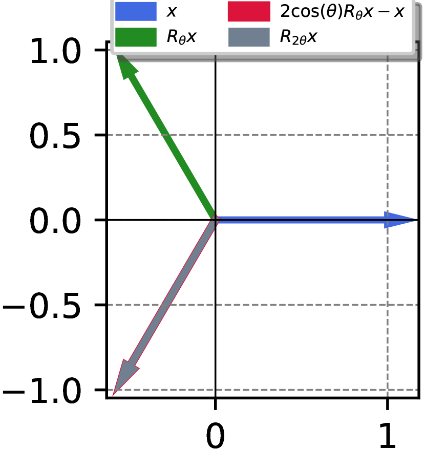
Figure 2: Trigonometric formula implemented by the Transformer in-context. The minima of the training loss correspond to implementing, up to multiplying factors: $2\cos{\theta}R_{\theta}-I_{2}=R_{2\theta}.$

We consider a self-attention module with $H$ heads, and we define the following assumption.

Assumption 3.

$A^{h}$ and $B^{h}$ are diagonal for all $h$: $A^{h}=\operatorname{diag}(a_{h})$ and $B^{h}=\operatorname{diag}(b_{h})$ with $(a_{h},b_{h})\in\mathbb{R}^{d}\times\mathbb{R}^{d}$.

Importantly, we impose the diagonal structure during training. This diagonal aspect reflects the diagonal property of the context matrices. Under assumptions 1 and 3, we have the following result.

Lemma 2.

Suppose assumptions 1 and 3. Writing $a_{h}=(a^{1}_{h},\cdots,a^{d}_{h})$ and $b_{h}=(b^{1}_{h},\cdots,b^{d}_{h})$ and letting $\mathtt{A}\coloneqq(a^{1},\cdots,a^{d})\in\mathbb{R}^{H\times d}$, and $\mathtt{B}\coloneqq(b^{1},\cdots,b^{d})$, one has for an input sequence $e_{1:T}=(1_{d},\lambda,\cdots,\lambda^{T-1})\in\mathbb{R}^{T\times d}:$

$$\mathcal{T}_{\theta}(e_{1:T})=\sum^{T}_{t=1}P_{T-1,t}[\mathtt{B}^{\top}\mathtt{A}]\lambda^{t-T+1}\odot\lambda^{t-1}.$$

For a full proof, refer to appendix A.4. Note that $\mathtt{A}$ and $\mathtt{B}$ correspond to the concatenation of diagonals $W_{K}^{h\top}W^{h}_{Q}$ and $W^{h}_{O}W^{h}_{V}$ along heads.
It is easily seen from Lemma 2 that the choice of $P_{T-1,t}^{*}=\delta_{t=T}$ and ${\mathtt{B}^{*}}^{\top}\mathtt{A}^{*}=I_{d}$ implies $\mathcal{T}_{\theta^{*}}(e_{1:T})=\lambda^{T}$, and therefore $\ell(\theta^{*})=0.$ We see that this requires at least $d$ heads. A natural question is whether there are other optimal solutions and how to characterize them. To answer this question, we investigate the case of unitary context matrices before moving to orthogonal ones. We consider these cases separately because they both lead to different in context mappings. We recall that $U(d)$ can be seen as a subset of $O(2d)$.

5.1 Unitary context matrices.

In this case, coefficients in the context matrices are drawn independently. This constrains the possible values for $\theta^{*}$ achieving zero loss. Indeed, we have the following result.

Proposition 3 (Unitary optimal in-context mapping).

Suppose assumptions 1 and 3. Any $\theta^{*}=(\mathtt{A}^{*},\mathtt{B}^{*},P^{*})$ achieving zero of the loss (3) satisfies $P^{*}_{T-1,t}=0$ if $t\neq T$, $P^{*}_{T-1,T}({\mathtt{B}^{*}}^{\top}\mathtt{A}^{*})_{ii}=1$, and $({\mathtt{B}^{*}}^{\top}\mathtt{A}^{*})_{ij}=0$ for $i\neq j.$ Therefore, one must have $H\geq d$. An optimal in-context mapping satisfies $\Gamma_{\theta^{*}}(e_{1:T})=\bar{e}_{T-1}\odot e_{T}$ and the predictive mapping $\psi_{\gamma}(e_{1:T})=\gamma\odot e_{T}$.

At $\ell(\theta^{*})=0$ one has $\mathcal{T}_{\theta^{*}}(e_{1:T})=\lambda^{T}$. We notice that $\mathcal{T}_{\theta^{*}}(e_{1:T})$ is a polynomial in the $\lambda_{i}$’s. Identifying the coefficients leads to the desired results. For a full proof, refer to appendix A.5. In particular, for $e_{1:T}=(1_{d},\lambda,\cdots,\lambda^{T-1})$, we have $\Gamma_{\theta^{*}}(e_{1:T})=\lambda$, and $\psi_{\Gamma_{\theta^{*}}}(e_{1:T})=\lambda\odot\lambda^{T-1}=\lambda^{T}$.

Orthogonality.

The equality $(\mathtt{B}^{\top}\mathtt{A})_{ij}=0$ for $i\neq j$ corresponds to an orthogonality property between heads. Indeed, to further understand what Proposition 3 implies in terms of learned model, let’s look at the particular case in which $H=d$ and, at optimality, $\mathtt{A}^{*}=\mathtt{B}^{*}=I_{d}$ and $P_{T-1,t}^{*}=\delta_{t=T}$. Therefore, the positional encoding selects the last token in the input sequence, hence learning the structure of the training data. In parallel, each attention matrix captures a coefficient in $\lambda$: $(\mathcal{T}_{\theta^{*}}(e_{1:T}))_{h}=\lambda_{h}\lambda_{h}^{T-1}$. When there are more than $d$ heads, some heads are useless, and can therefore be pruned. Such a finding can be related to the work of Michel et al. (2019), where the authors experimentally show that some heads can be pruned without significantly affecting the performance of Transformers. Orthogonality in the context of Transformers was also investigated by directly imposing orthogonality between the outputs of each attention head (Lee et al., 2019) or on attention maps (Chen et al., 2022; Zhang et al., 2021). The ability of the positional encoding to recover the spatial structure was already shown by Jelassi et al. (2022), which studies Vision Transformers (Dosovitskiy et al., 2020).

Convergence of gradient descent.

Now that we have characterized all the global minima of the loss (3), we can study the convergence of the optimization process. We have the following Proposition, which shows that the population loss (3) writes as a quadratic form in $\mathtt{B}^{\top}\mathtt{A}$ and $P$, which enables connections with matrix factorization.

Proposition 4 (Quadratic loss).

Under assumptions 1 and 3, the loss reads

$$\ell(\mathtt{A},\mathtt{B},P)=\sum_{T=2}^{T_{max}}l(\mathtt{C},P_{T-1})$$

and $l(\mathtt{C},p)=\|p\|^{2}_{2}\|\mathtt{C}\|^{2}_{F}+p_{T-1}^{2}S(\mathtt{C}^{\top}\mathtt{C})-2\mathrm{Tr}(\mathtt{C})p_{T}+d$, where $\mathtt{C}=\mathtt{B}^{\top}\mathtt{A}$, and $S$ is the sum operator.

See Appendix A.6 for a proof. For an optimal $P^{*}$, the loss is (up to rescaling): $\ell(\mathtt{A},\mathtt{B})=\|\mathtt{B}^{\top}\mathtt{A}-I\|^{2}_{F},$ for which we can use Theorem 2.2 of Nguegnang et al. (2021) to argue that for almost all initial values, gradient flow on $L$ will converge to a global minimum, that is $\mathtt{B}^{\top}\mathtt{A}=I_{d}$. When training is also done on $p\coloneqq P_{T-1,T}$, the loss is then $L(\mathtt{A},\mathtt{B},p)=\|p\mathtt{B}^{\top}\mathtt{A}-I\|^{2}_{F}$. Note that convergence of gradient descent in $(\mathtt{A},\mathtt{B},p)$ on $L$ to a global minimum is an open problem, for which a conjecture (Nguegnang et al., 2021; Achour et al., 2021) states that for almost all initialization, $(\mathtt{A},\mathtt{B},p)$ will converge to a global minimum of $\ell$. We provide evidence for global convergence in Figure 3. Yet, we have the following result in the scalar case $H=d=1$. Its proof is in Appendix A.7.

Proposition 5.

Consider the loss $\ell(a,b,p)=(pab-1)^{2}$. Suppose that at initialization, $|pab-1|<1$. Then gradient flow on $(a,b,p)$ converges to a global minimum satisfying $a^{*}b^{*}p^{*}=1$.

5.2 Orthogonal context matrices.

We now turn to the case where the context matrices are in $\mathcal{C}_{O}$. We recall that this imposes that the $\lambda_{i}$ are pairwise conjugate. Therefore, the dimension d is even, and we write it $d=2\delta$. The context matrices are therefore rotations. This property changes the optimization landscape and other solutions are possible, as shown in the following lemma.

Lemma 3.

Suppose assumptions 1, 3. If $P^{*}_{T-1,T-1}=-1$, $P^{*}_{T-1,T}=2$ and $0$ otherwise, and ${\mathtt{B}^{*}}^{\top}\mathtt{A}^{*}=\frac{1}{2}\operatorname{diag}(J,\cdots,J)$, with $J\in\mathbb{R}^{2\times 2}$ and $J_{ij}=1$ for all $i,j$, then $\mathcal{T}_{\theta^{*}}(e_{1:T})=\lambda^{T}.$

For a full proof, refer to appendix A.5. In this case, $H=\delta$ heads are sufficient to reach zero population loss. In fact, the optimal parameters can be exactly characterized.

Proposition 6 (Orthogonal optimal in-context mapping).

Suppose assumptions 1 and 3. Any $\theta^{*}=(\mathtt{A}^{*},\mathtt{B}^{*},P^{*})$ with $\ell(\theta^{*})=0$ in (3) satisfies, denoting $\mathtt{C}^{*}={\mathtt{B}^{*}}^{\top}\mathtt{A}^{*}$ and $p^{*}=P^{*}_{T-1}$: $p^{*}_{t}=0$ if $t<T-1$, $p^{*}_{T}\mathtt{C}^{*}_{i,i}=1$, $p^{*}_{T}\mathtt{C}^{*}_{2i-1,2i}+(\mathtt{C}^{*}_{2i-1,2i-1}+\mathtt{C}^{*}_{2i-1,2i})p^{*}_{T-1}=0$, $p^{*}_{T}\mathtt{C}^{*}_{2i,2i-1}+(\mathtt{C}^{*}_{2i,2i}+\mathtt{C}^{*}_{2i,2i-1})p^{*}_{T-1}=0$, $\mathtt{C}^{*}_{2i-1,j}=\mathtt{C}^{*}_{2i,j}=0$ for $j\neq 2i-1,2i$. An optimal in-context mapping is then, for $e_{t}=\lambda^{t-1}$: $\Gamma_{\theta^{*}}(e_{1:T})=\lambda^{2}$, and the predictive mapping $\psi_{\Gamma_{\theta^{*}}(e_{1:T})}(e_{1:T})=\lambda^{2}\odot e_{T-1}=\lambda^{T}$.

Similarly to Proposition 3, we identify the coefficients of a polynomial, with careful inspection of terms involving pairwise conjugate contexts $(\lambda_{i},\bar{\lambda_{i}})$ Similarly to Proposition 3, this result indicates an orthogonal property between heads. A closer look at the computation of $\Gamma_{\theta^{*}}$ reveals that the relation implemented in-context by the Transformer in Proposition 6 is an extension of a known formula in trigonometry: $2\cos{\theta}R_{\theta}-I_{2}=R_{2\theta}$, with $R_{\theta}$ the rotation of parameter $\theta$ in $\mathbb{R}^{2}$ (see Figure 2). Importantly, when $\delta\leq H<2\delta=d$, the optimal $\mathtt{C}^{*}$ in Proposition 6 is of rank $\delta$, which corresponds to Lemma 3. However, when $H\geq d$, full rank solutions are achievable.

Under the assumptions of Proposition 3, the population loss (3) is also a quadratic form in $P$ and $\mathtt{B}^{\top}\mathtt{A}$. Similarly to Proposition 4, global convergence results of gradient descent on such loss function are still an open problem (Achour et al., 2021). We provide experimental evidence for convergence in Figure 3.

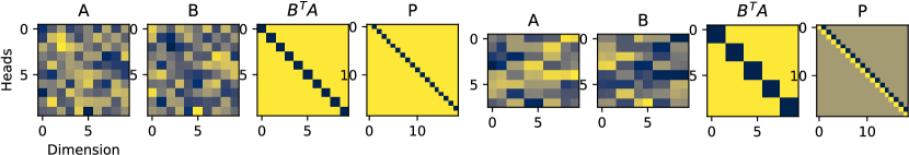
Figure 3: Matrices $\mathtt{A}$, $\mathtt{B}$, $\mathtt{B}^{\top}\mathtt{A}$ and $P$ after training model (6) on loss (3) with random initialization. We take $d=10$ and $T=15$. Left: Unitary context case with $H=10.$ Right: Orthogonal context case, with $H=8<d$, which leads to low rank $\mathtt{B}^{\top}\mathtt{A}$. In both cases, we obtain arbitrary small final loss. We recover parameters corresponding to our Propositions 3 and 6. Note that the coefficients on the sub-diagonal of $P$ indicate, as we consider $\tau=T-1$, that the last token $e_{T}$ (left) or the last two tokens $e_{T-1}$ and $e_{T}$ (right), are used to make the prediction of the next token $e_{T+1}$ (which is always masked).

5.3 Positional encoding only attention.

We end this section by investigating the impact of the context distribution on the trained positional encoding $P$. For this, we consider a positional-encoding-only Transformer, that is, we fix $\mathtt{B}^{\top}\mathtt{A}=I_{d}$. In this case, the problem decomposes component-wise, and we only need to consider the $d=1$ case. We therefore consider the AR process $s_{t+1}=\lambda s_{t}$ for $|\lambda|=1$. We break the symmetry of the context distribution: for $\mu\geq 1$ and $\theta\sim\mathcal{U}(0,2\pi),$ we define $\lambda=e^{i\theta/\mu}$. We denote $\mathcal{W}(\mu)$ the corresponding distribution. Therefore, we focus on the optimization problem:

$$\min_{p\in\mathbb{R}^{T}}l(p)\coloneqq\mathbb{E}_{\lambda\sim\mathcal{W}(\mu)}|\sum_{t=1}^{T}p_{t}\lambda^{2t-T}-\lambda^{T}|^{2}.$$ (7)

Here again, the same proof as for Proposition 3 shows that the optimal positional encoding is $p^{*}=\delta_{t=T}$, meaning that we make the prediction of the next token using the last token in the context. However, depending on $\mu$, (7) can be ill conditioned.

Proposition 7 (Conditioning).

The Hessian $H\in\mathbb{R}^{T\times T}$ of $l$ in (7) is given by

$$H_{t,t’}=\frac{\mu}{4\pi(t’-t)}\sin(4(t’-t)\frac{\pi}{\mu}).$$

Denoting $\sigma_{1}(\mu)\geq\dots\sigma_{T}(\mu)$ its eigenvalues, one has $\sigma_{1}(\mu)\to T$ and $\sigma_{t>1}(\mu)\to 0$ as $\mu\to+\infty$.

Therefore, for large $\mu$, $H$ in Proposition 7 is poorly conditioned. In such a setting, gradient descent, even with a large number of iterations, induces a $\ell_{2}$ regularization (Yao et al., 2007). As a consequence, approximate solutions computed by gradient descent significantly deviate from the optimal $p^{*}$. As demonstrated experimentally in Figure 8 and §6, the effect of this regularization is a spatial smoothing of the positional encoding, which leads to entirely different in-context mappings $\Gamma$, hence showing the effect of the optimization process on the in-context autoregressive learning abilities of Transformers.

6 Experiments

In this section, we illustrate and extend our results through experiments. Our code in Pytorch (Paszke et al., 2017) and JAX (Bradbury et al., 2018) will be open-sourced. We use the standard parametrization of Transformers, that is we train on $(W_{Q},W_{K},W_{V},W_{O})$.

Validation of the token encoding choice.

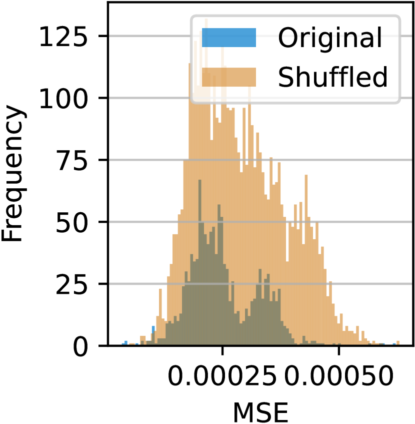
Figure 4: Histograms of the mean squared errors (MSE) when fitting an AR process to sequences in $D$ (original, in blue) or $D_{\mathrm{shuffle}}$ (shuffled, in orange). We only display MSEs bigger than a threshold of $10^{-12}$.

Throughout the paper, we make the assumption that the $s_{1:T}$ are generated following an AR process $s_{t+1}=Ws_{t}$. We provide empirical justification for using an AR process to model real-word sentences, by showing that such a process better explains real data than random ones. We use the nltk package (Bird et al., 2009), and we employ classic literary works, specifically ’Moby Dick’ by Herman Melville sourced from Project Gutenberg. We use the tokenizer and word embedding layer of a pre-trained GPT-2 model (Radford et al., 2019), and end up with about $325000$ token representations in dimension $d=1280$, that we reformat in a dataset $D$ of shape $(n,T,d)$, where $T=5$ (we keep the relative order of each token). We also consider a shuffled counterpart of $D$ where the shuffling is done across the first two dimensions. In other words, we create a dataset $D_{\mathrm{shuffle}}$ from a permutation of the tokens of the book.
We then fit AR processes for each sequence in the two datasets using loss (5), which we minimize by solving a linear system. It should be noted that the problem remains non-trivial for some sequences, despite $T$ being significantly smaller than $d$. This complexity arises because certain sequences might contain identical elements with differing successors or predecessors. We hypothesize that when sequences are shuffled, the number of such inconsistencies increases since the language’s structure is lost. This hypothesis is validated in Figure 4, where we display the histograms of the fitting losses when they are bigger than $10^{-12}.$ There are $4$ times more sequences with such an error for the shuffled dataset than for the original. This shows that the AR process is better suited when data present some semantics.

Augmented setting.

We investigate whether the results of §4 still hold without assumptions 1 and 2. We consider the model (4) on the augmented tokens $e_{t}=(0,s_{t},s_{t-1})$. We iterate relation (4) with several layers, using layer normalization (Ba et al., 2016). We consider depth values from $1$ to $6$. We generate a dataset with $n=2^{14}$ sequences with $T_{\mathrm{max}}=50$ and $d=5$ (therefore $e_{t}\in\mathbb{R}^{15}$) for training. We test using another dataset with $2^{10}$ sequences of the same shape. We train for $2000$ epochs with Adam (Kingma & Ba, 2014) and a learning rate of $5\times 10^{-3}$ to minimize the mean squared error (MSE) $\min\ell(\Theta)\coloneqq\sum_{T=2}^{T_{\mathrm{max}}}\frac{1}{n}\sum_{i=1}^{n}\|\mathcal{T}^{L}_{\Theta}(e^{i}_{1:T})-s^{i}_{T}\|^{2}$, where $\mathcal{T}^{L}_{\theta}$ correspond to $L$ layers of (4) (we apply the forward rule $L$ times, and then consider the section of first $d$ coordinates). We compare the error with $L$ steps of gradient descent on the inner loss (5), with a step-size carefully-chosen to obtain the fastest decrease. We find out that even though the first Transformer layers are competitive with gradient descent, the latter outperforms the Transformer by order of magnitudes when $L\geq 3$. Results are displayed in Figure 5. The fact that several steps of gradient descent outperform the same number of $\mathcal{T}_{\theta}$ layers is not surprising, as Proposition 2 does not generalize to more than one layer.

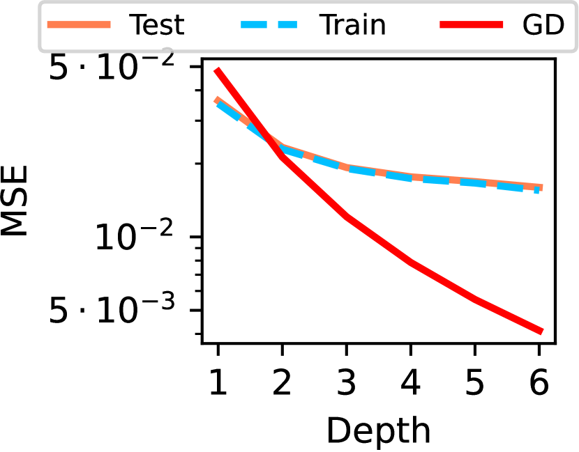
Figure 5: Evolution of the mean squared errors (MSE) with depth $L$. We compare with $L$ steps of gradient descent (GD) on the inner loss (5).

Non-Augmented setting.

We now investigate whether the results of §5 still hold without assumptions 1 and 3. We consider the model $\mathcal{T}_{\theta}$ in (6). We parameterize the positional encoding in the linear Transformer equation (6) using the $\mathrm{softmax}$ of a positional attention-only similarity cost matrix with learnable parameters $W_{Q_{\mathrm{pos}}}$ and $W_{K_{\mathrm{pos}}}$: $P_{t,t^{\prime}}=\mathrm{softmax}(\langle W_{Q_{\mathrm{pos}}}p_{t}|W_{K_{\mathrm{pos}}}p_{t^{\prime}}\rangle),$ as we found it to stabilize the training process. We use a similar dataset as in the previous section, i.e., a training set with $2^{14}$ sequences, each with $50$ elements of dimension $d=10$, and we test using another dataset with $2^{10}$ sequences of the same shape.

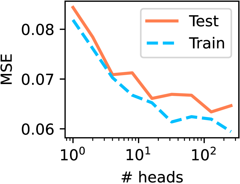
Figure 6: Evolution of the mean squared errors (MSE) with the number of heads.

We train models $\mathcal{T}_{\theta}$ in (6) for $200$ epochs with different numbers of heads. We use the Adam optimizer with a learning rate of $10^{-2}$. Without further modification, we do not observe a significant gain as the number of heads increases. However, when duplicating the data along the dimension axis, that is $e_{t}\coloneqq(s_{t},s_{t})$, we observe a significant improvement, as illustrated in Figure 6. To further relate our experimental findings to our theory, we also exhibit an orthogonality property between heads after training. For this, we take $d=5$ to ease the visualization, and initialize each parameter equally across heads but add a small perturbation $.05\times\mathcal{N}(0,1)$ to ensure different gradient propagation during training. We then train the model and compare the quantity $(\sum_{h=1}^{H}(B^{\top}_{h}B_{h}))_{(i,j)}$ after training and at initialization. Note that it corresponds to a measure of orthogonality of heads. Results are displayed in Figure 7. We observe that after training, an orthogonality property appears. In addition, as we are duplicating the tokens across dimensions, we can see that heads become specialized in attending to some coordinates across tokens.

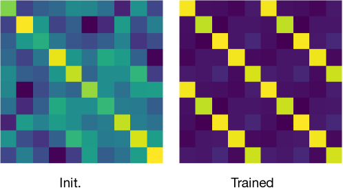
Figure 7: Matrices $(\sum_{h=1}^{H}(B^{\top}_{h}B_{h}))_{(i,j)}\in\mathbb{R}^{10\times 10}$ at initialization and after training. The trained parameters lead to an orthogonality between heads, as predicted by our theory.

Change in the context distribution.

We consider the setting of §5.3, using the empirical loss counterpart of (7), averaged over $T\in\{2,\cdots,T_{\mathrm{max}}\}$. We generate a dataset with $10^{4}$ examples and $T_{\max}=30$. We train our positional encoding-only model with gradient descent, and stop training (early stopping) when the loss is smaller than $10^{-3}$. We initialize $P_{t,t^{\prime}}=0$. Results are in Figure 8, where we mask coefficients $P_{T-1,T}$ (which are close to $1$ after training) in the display to investigate the behavior of the extra coefficients. We observe that the trained positional encoding exhibits an invariance across diagonals. Importantly, each row $P_{t}$ has a smooth behavior with $t^{\prime}$, that we compare to absolute cosine positional encodings (Vaswani et al., 2017).

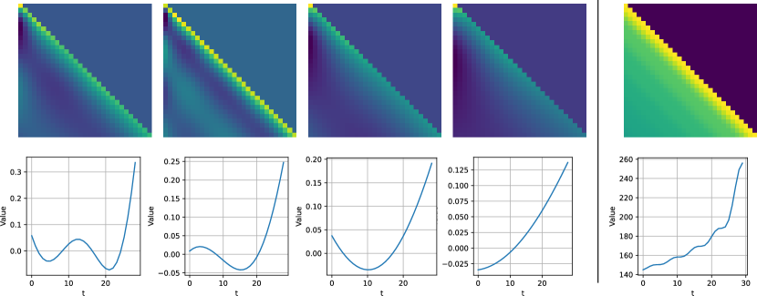
Figure 8: Left: Positional encodings after training for $\mu\in\{50,100,200,300\}$. The first raw corresponds to the matrix P, and the second raw to a plot of its last raw. Right: Comparison with the cosine absolute positional encoding standardly used in machine translation (Vaswani et al., 2017) (we display $pp^{\top}$). In both cases, we observe an invariance across diagonals. In addition, for high $\mu$ (i.e. small variations of the context), the most recent tokens are more informative, as imposed by the inductive prior of the cosine positional encoding.

Conclusion

In this work, we study the in-context autoregressive learning abilities of linear Transformers to learn autoregressive processes of the form $s_{t+1}=Ws_{t}$. In-context autoregressive learning is decomposed into two steps: estimation of $W$ with an in-context map $\Gamma$, followed by a prediction map $\psi$. Under commutativity and parameter structure assumptions, we first characterized $\Gamma$ and $\psi$ on augmented tokens, in which case $\Gamma$ is a step of gradient descent on an inner objective function. We also considered non-augmented tokens, and showed that $\Gamma$ corresponds to an non-trivial geometric relation between tokens, enabled by an orthogonality between trained heads and learnable positional encoding. We also studied positional-encoding-only attention, and showed that approximate solutions of minimum $\ell_{2}$ norm are favored by the optimization. Moving beyond commutativity assumptions, we presented empirical pieces of evidence that our theoretical findings hold in the general case.

Regarding future work, investigating the case where $\tau=T$ in the non-augmented setting would lead to approximated in-context mappings, where achieving zero loss is no longer possible. This investigation would provide further insights into the role of positional encoding in estimating $W$ in-context.

Appendix A Proofs

In what follows, as we consider complex numbers, we use the hermitian product over $\mathbb{C}^{d},$ that is $\langle\alpha,\beta\rangle\coloneqq\beta^{\star}\alpha=\sum_{i}\alpha_{i}\bar{\beta_{i}}$.

We denote $\mathcal{U}^{d}=\{\lambda\in\mathbb{C}^{d}||\lambda_{i}|=1\forall i\in\{1,\cdots,d\}\}.$

A.1 Proof of Lemma 1.

Proof.

Let, for $s\in\mathbb{R}^{d}$, $W^{1}_{V}s\coloneqq(0,s,0)\in\mathbb{R}^{3d}$ and $W^{2}_{V}s\coloneqq(0,0,s)$.

We now simply consider for $h\in\{1,2\}$:

$$\mathcal{A}^{h}_{t,:}=\mathrm{softmax}(P^{h}_{t,:}).$$

We can choose $P^{1}$ and $P^{2}$ such that ${A}^{1}_{t,t^{\prime}}\simeq\delta_{t^{\prime}=t}$ and ${A}^{2}_{t,t^{\prime}}\approx\delta_{t^{\prime}=t-1}.$ Then

$$\sum_{h=1}^{2}\sum_{t^{\prime}=1}^{t}\mathcal{A}^{h}_{t,t^{\prime}}W^{h}_{V}s_{t^{\prime}}\simeq(0,s_{t},s_{t-1})=e_{t}.$$

∎

A.2 Proof of Proposition 1

Proof.

We briefly recall the reasoning as presented in Von Oswald et al. (2023b), and consider the case $W_{0}=0$ for simplicity. See Von Oswald et al. (2023b) for a full proof. Let

Then the section vector of the first $d$ coordinates in (4) is $-\eta\sum_{t=1}^{T}s_{t}s^{\top}_{t-1}s_{T}.$

Since the gradient of $L$ at $W_{0}=0$ is:

$$\nabla_{W}L(W_{0})=2\sum_{t=1}^{T-1}(s_{t+1})s^{\top}_{t},$$

this corresponds to a single step of gradient descent starting from $W_{0}=0$. ∎

A.3 Proof of Proposition 2

We first consider the following lemma.

Lemma 4.

Under assumptions 1 and 2, the loss of the linear Transformer writes:

$$\ell((a_{i}),(b_{i}))=\mathbb{E}_{\lambda}{\sum_{T=2}^{T_{\mathrm{max}}}\sum_{i=1}^{d}|\sum_{t,j,\alpha\in\mathcal{A},\beta\in\mathcal{B}}c_{\alpha,\beta}\lambda^{T-t-1-\alpha}_{j}\lambda^{t+\beta}_{i}-\lambda^{T}_{i}|^{2}}$$ (9)

with $\mathcal{A}=\{-1,0,1\}$ and $\mathcal{B}=\{-1,0\}.$ We have $c_{\alpha,\beta}=u_{\alpha}v_{\beta}$ for $u_{0}=a_{1}+a_{4}$, $u_{1}=a_{2}$, $u_{-1}=a_{3}$, $v_{0}=b_{1}$ and $v_{-1}=b_{2}$.

Proof.

One has $Ae_{T}=(0,a_{1}s_{T}+a_{2}s_{T-1},a_{3}s_{T}+a_{4}s_{T-1}).$ Therefore one has $\langle Ae_{T},e_{t}\rangle=a_{1}s_{t}^{\star}s_{T}+a_{2}s_{t}^{\star}s_{T-1}+a_{3}s_{t-1}^{\star}s_{T}+a_{4}s_{t-1}^{\star}s_{T-1}.$ Since $(Be_{t})_{1:d}=b_{1}s_{t}+b_{2}s_{t-1},$ one obtains

$$\mathcal{T}_{\theta}(e_{1:T})_{i}=\sum_{t}(a_{1}s_{t}^{\star}s_{T}+a_{2}s_{t}^{\star}s_{T-1}+a_{3}s_{t-1}^{\star}s_{T}+a_{4}s_{t-1}^{\star}s_{T-1})(b_{1}s_{t}+b_{2}s_{t-1}).$$

Developing, we obtain

$$\mathcal{T}_{\theta}(e_{1:T})_{i}=\sum_{t,j,\alpha\in\mathcal{A},\beta\in\mathcal{B}}c_{\alpha,\beta}\lambda^{T-1-t-\alpha}_{j}\lambda^{t+\beta}_{i},$$

which implies the result. ∎

Using the notations of Lemma 4, Proposition 2 now writes as follows.

Proposition 8 (In-context autoregressive learning with gradient-descent.).

Suppose assumptions 1 and 2. The loss is minimal for $c_{\alpha,\beta}=0$ if $(\alpha,\beta)\neq(-1,0)$ and $c_{-1,0}=\frac{\sum_{T=2}^{T_{\mathrm{max}}}T}{\sum_{T=2}^{T_{\mathrm{max}}}(T^{2}+(d-1)T)}$. Therefore, the optimal in-context map $\Gamma_{\theta^{*}}$ is one step of gradient descent starting from the initialization $\lambda=0$, with a step size asymptotically equivalent to $\frac{3}{2T_{\max}}$ with respect to $T_{\mathrm{max}}$.

Proof.

We develop the term in the sum in (9):

$$\begin{split}&|\sum_{t,j,\alpha\in\mathcal{A},\beta\in\mathcal{B}}c_{\alpha,\beta}\lambda^{T-t-\alpha}_{j}\lambda^{t+\beta}_{i}-\lambda^{T+1}_{i}|^{2}\\ &=\sum_{t_{1},j_{1},\alpha_{1},\beta_{1},t_{2},j_{2},\alpha_{2},\beta_{2}}c_{\alpha_{1},\beta_{1}}c_{\alpha_{2},\beta_{2}}\lambda^{T-t_{1}-\alpha_{1}}_{j_{1}}\lambda^{-T+t_{2}+\alpha_{2}}_{j_{2}}\lambda^{t_{1}-t_{2}+\beta_{1}-\beta_{2}}_{i}\\ &-2\mathrm{Real}(\sum_{t,j,\alpha\in\mathcal{A},\beta\in\mathcal{B}}c_{\alpha,\beta}\lambda^{T-t-\alpha}_{j}\lambda^{t+\beta}_{i}\lambda_{i}^{-T-1})+1.\end{split}$$

We now need to compute the expectations of the first two terms in the sum.

Because $\mathbb{E}{(\lambda^{k}_{i})}=\delta_{k=0}$ and the $\lambda$ are i.i.d., most terms will be zeros.

For the first term, by looking at the different possible values for $(j_{1},j_{2},i)$, we see that all the terms that do not satisfy $\alpha_{1}-\alpha_{2}=\beta_{1}-\beta_{2}$ will lead to $0$ expectation. The expectation of the first term then writes, for some constant $K_{T}$: $K_{T}\sum_{\alpha_{1}-\alpha_{2}=\beta_{1}-\beta_{2}}c_{\alpha_{1},\beta_{1}}c_{\alpha_{2},\beta_{2}}.$

For the second term, we get $-2Tc_{-1,0}$. Isolating the terms in $c_{-1,0}$, we get

$$K_{T}\sum_{\alpha_{1}-\alpha_{2}=\beta_{1}-\beta_{2},(\alpha_{1},\alpha_{2},\beta_{1},\beta_{2})\neq(-1,-1,0,0)}c_{\alpha_{1},\beta_{1}}c_{\alpha_{2},\beta_{2}}+K_{T}c^{2}_{-1,0}-2Tc_{-1,0}+1=$$

$$K^{(1)}_{T}(c_{-1,-1}+c_{0,0})^{2}+K^{(2)}_{T}(c_{1,0}+c_{0,-1})^{2}+K^{(3)}_{T}c^{2}_{1,-1}+K_{T}c^{2}_{-1,0}-2Tc_{-1,0}+1,$$

where the constants $K^{(i)}_{T}$ are non-negative.

We obtain a second-order polynomial in the $c_{\alpha,\beta}$’s. At optimality, one necesseraly has $c_{-1,0}\neq 0$ and $c_{-1,-1}+c_{0,0}=0$, $c_{1,0}+c_{0,-1}=0$, $c^{2}_{1,-1}=0$. It follows that $a_{1}+a_{4}=0$, $a_{2}=0$, $a_{3}\neq 0$, $b_{1}\neq 0$ and $b_{2}=0$. Therefore, $c_{\alpha,\beta}=0$ if $(\alpha,\beta)\neq(-1,0).$

We now denote $\alpha=a_{3}b_{1}$. Replacing the zero terms in loss (9), we obtain

$$d\sum^{T_{\mathrm{max}}}_{T=2}\left(\alpha^{2}(T^{2}+(d-1)T)-2\alpha T+1\right),$$

for which the argmin is given by

$$\alpha^{*}=\frac{\sum_{T=2}^{T_{\mathrm{max}}}T}{\sum_{T=2}^{T_{\mathrm{max}}}(T^{2}+(d-1)T)}.$$

∎

A.4 Proof of Lemma 2.

Proof.

For a given input sequence $s_{1:T}=(s,\lambda\odot s,\cdots,\lambda^{T-1}\odot s)$, with context $\lambda\in\mathcal{U}^{d}$, one has

$$\mathcal{T}_{\theta}(e_{1:T})=\sum_{t=1}^{T}P_{T-1,t}\sum_{h=1}^{H}\langle\lambda^{t-1}\odot s,a_{h}\odot\lambda^{T-2}\odot s\rangle b_{h}\odot\lambda^{t-1}\odot s.$$

We have

$$(\langle\lambda^{t-1}\odot s,a_{h}\odot\lambda^{T-2}\odot s\rangle b_{h}\odot\lambda^{t-1}\odot s)_{i}=\sum_{j=1}^{d}{a^{j}_{h}\lambda^{2-T}_{j}\lambda^{t-1}_{j}b^{i}_{h}\lambda^{t-1}_{i}}.$$

Since we precisely have

$$([\mathtt{B}^{\top}\mathtt{A}]\lambda^{t-T+1}\odot\lambda^{t-1})_{i}=\sum_{j=1}^{d}\sum_{h=1}^{H}{b^{i}_{h}a^{j}_{h}\lambda^{t-T+1}_{j}\ \lambda^{t-1}_{i}},$$

this gives us the desired result.

∎

A.5 Proof of Proposition 3

Proof.

Let us suppose that we have an optimal solution $\theta^{*}$ such that $l(\theta^{*})=0.$ Therefore, for almost all $\lambda\in\mathcal{U}^{d}$ and $s_{t}=\lambda^{t-1}$, one has $\mathcal{T}_{\theta}(s_{1:T})=\lambda^{T}$. Then, $\forall i\in\{1,\cdots,d\}$:

$$\sum^{T}_{t=1}P_{T-1,t}\sum_{j=1}^{d}\mathtt{C}_{ij}\lambda^{t-T+1}_{j}\lambda^{t-1}_{i}=\lambda_{i}^{T}.$$

By identifying the coefficients of the polynomial in the $\lambda_{i}$’s, we see that one must have for all $T$ that $P_{T-1,t}=0$ if $t\neq T$, and for all $1\leq i\leq d$, $p_{T-1,T}\mathtt{C}_{ii}=1$, and $\mathtt{C}_{ij}=0$ for $i\neq j.$

An optimal in-context mapping is then obtained by considering the forward rule of $\mathcal{T}_{\theta^{*}}$ for optimal parameters. One gets:

$$\mathcal{T}_{\theta^{*}}(e_{1:T})=(\bar{e}_{T-1}\odot e_{T})\odot(e_{T}).$$

The results follows.

∎

A.6 Proof of Proposition 4

Proof.

The loss writes

$$\ell(\theta)=\sum_{T=2}^{T_{\mathrm{max}}}\mathbb{E}_{\operatorname{diag}{\lambda}\sim\mathcal{W}}\|\sum^{T}_{t=1}P_{T-1,t}[\mathtt{C}]\lambda^{t-T+1}\odot\lambda^{t-1}-\lambda^{T}\|^{2}.$$

We compute the expectation of each term in the sum by first developing it.

One has

$$\|\sum^{T}_{t=1}P_{T-1,t}[\mathtt{B}^{\top}\mathtt{A}]\lambda^{t-T+1}\odot\lambda^{t-1}-\lambda^{T}\|^{2}=\sum_{t,t^{\prime}}P_{T-1,t}P_{T-1,t^{\prime}}\sum_{i,j,k}\mathtt{C}_{ij}\mathtt{C}_{ik}\lambda_{j}^{T-t-1}\lambda_{k}^{t^{\prime}-T+1}\lambda_{i}^{t^{\prime}-t}$$

$$-2\mathrm{Real}(\sum_{t}P_{T-1,t}\sum_{i,j}\mathtt{C}_{ij}\lambda_{j}^{T-t-1}\lambda_{i}^{T-t+1})+d.$$

Looking at the expectation of the first term

$$\sum_{t,t^{\prime}}P_{T-1,t}P_{T-1,t^{\prime}}\sum_{i,j,k}\mathtt{C}_{ij}\mathtt{C}_{ik}\mathbb{E}(\lambda_{j}^{T-t-1}\lambda_{k}^{t^{\prime}-T+1}\lambda_{i}^{t^{\prime}-t}),$$

we see that one has to calculate for $t,t^{\prime},i,j,k$

$$\mathbb{E}(\lambda_{j}^{T-t-1}\lambda_{k}^{t^{\prime}-T+1}\lambda_{i}^{t^{\prime}-t}).$$

When $j\neq k$, it is $\delta_{t^{\prime}=t=T-1}.$ When $j=k$ it is $\delta_{t^{\prime}=t}.$

Therefore

$$\sum_{t,t^{\prime}}P_{T-1,t}P_{T-1,t^{\prime}}\sum_{i,j,k}\mathtt{C}_{ij}\mathtt{C}_{ik}\mathbb{E}(\lambda_{j}^{T-t-1}\lambda_{k}^{t^{\prime}-T+1}\lambda_{i}^{t^{\prime}-t})=\sum_{t=t^{\prime}}P^{2}_{T-1,t}\sum_{i,j}\mathtt{C}^{2}_{ij}+P^{2}_{T-1,T-1}\sum_{i,j,k}\mathtt{C}_{i,j}\mathtt{C}_{i,k}=$$

$$\|P_{T-1}\|^{2}\|\mathtt{C}\|_{F}^{2}+P^{2}_{T-1}S(\mathtt{C}^{\top}\mathtt{C}).$$

Similarly, the second term is

$$-2\mathbb{E}(\mathrm{Real}(\sum_{t}P_{T-1,t}\sum_{i,j}\mathtt{C}_{ij}\lambda_{j}^{T-t-1}\lambda_{i}^{T-t+1}))=-2\mathrm{Tr}(\mathtt{C}).$$

This concludes the proof.

∎

A.7 Proof of Proposition 5

Proof.

Through Nguegnang et al. (2021); Achour et al. (2021), we know that $(a,b,p)$ are bounded and converge to a stationary point $(a^{*},b^{*},p^{*})$.

The stationary points are either $p^{*}a^{*}b^{*}=1$ (global) or such that $a^{*}b^{*}=0$, $a^{*}p^{*}=0$, $b^{*}p^{*}=0$. In particular, we necessarily have $p^{*}a^{*}b^{*}=0$ for non global minima.

As the energy decreases, it cannot converge to $p^{*}a^{*}b^{*}=0$ since then $|p^{*}a^{*}b^{*}-1|=1$, which is bigger than $\ell$ at initialization.

Therefore, the only remaining critical points must satisfy $p^{*}a^{*}b^{*}=1$ and are thus global.

∎

A.8 Proof of Lemma 3

Proof.

For the announced parameters, the problem simply decomposes in sub-problems in dimension $2$. Indeed, we have for all $i\in\{1,\delta\}$:

$$(\mathcal{T}_{\theta^{*}}(e_{1:T}))_{2i-1}=-\frac{1}{2}(\lambda_{2i-1}^{0}+\bar{\lambda}_{2i-1}^{0})\lambda_{2i-1}^{T-2}+(\lambda_{2i-1}^{1}+\bar{\lambda}_{2i-1}^{1})\lambda_{2i-1}^{T-1}=\lambda_{2i-1}^{T-2}(-1+\lambda_{2i-1}^{2}+1)=\lambda_{2i-1}^{T}.$$

Similarly,

$$(\mathcal{T}_{\theta^{*}}(e_{1:T}))_{2i}=\lambda_{2i}^{T}.$$

∎

A.9 Proof of Proposition 6

Proof.

The proof is similar to Proposition A.5, by regrouping each $\lambda_{i}$ with $\bar{\lambda}_{i}$ and identifying coefficients in two polynomials. More precisely, one must have

$$\sum^{T}_{t=1}P_{T-1,t}\sum_{j=1}^{d}\mathtt{C}_{2i-1,j}\lambda^{t-T+1}_{j}\lambda^{t-1}_{2i-1}=\lambda_{2i-1}^{T}.$$

Therefore, isolating terms in $\lambda_{2i-1}$ (recall that $\lambda_{2i}=1/{\lambda_{2i-1}}$), and developing, we get, noting $p\coloneqq P_{T-1}$:

$$\mathtt{C}_{2i-1,2i-1}(\sum_{t<T-1}p_{t}\lambda^{2t-T}_{2i-1}+p_{T-1}\lambda^{T-2}_{2i-1}+p_{T}\lambda^{T}_{2i-1})+\sum_{t}p_{t}\mathtt{C}_{2i-1,2i}\lambda^{T-2}_{2i-1}=\lambda^{T}_{2i-1}.$$

Identifying gives $\mathtt{C}_{2i-1,2i-1}+\mathtt{C}_{2i-1,2i}p_{T-1}+\mathtt{C}_{2i-1,2i}p_{T}=0$, $\mathtt{C}_{2i-1,2i-1}p_{T}=1$ and $p_{t<T-1}=0$.

Similarly, on the conjugates, $\mathtt{C}_{2i,2i}+\mathtt{C}_{2i,2i-1}p_{T-1}+\mathtt{C}_{2i,2i-1}p_{T}=0$, $\mathtt{C}_{2i,2i}p_{T}=1$.

Identifying the other terms gives $C_{2i,j}=C_{2i-1,j}=0$ for $j\neq 2i$ and $j\neq 2i-1$.

∎

A.10 Proof of Proposition 7

Proof.

One has that the second order term in the quadratic form (7) writes

$$\langle p|Hp\rangle=\sum_{t,t^{\prime}}p_{t}p_{t^{\prime}}\mathbb{E}_{\lambda\sim\mathcal{W}(\mu)}\lambda^{2(t^{\prime}-t)}.$$

We can actually calculate this expectation in close form. Writing $\alpha=\frac{2\pi}{\mu}$, it gives

$$\mathbb{E}_{\lambda\sim\mathcal{W}(\mu)}\lambda^{2(t^{\prime}-t)}=\frac{1}{\alpha}\int_{0}{\alpha}e^{2i\theta(t^{\prime}-t)d\theta},$$

which gives $\frac{i}{2\alpha(t^{\prime}-t)}[1-e^{2i(t^{\prime}-t)\alpha}]$ if $t\neq t^{\prime}$ and $1$ otherwise. Since $\langle p|Hp\rangle$ is real, we can identify the real parts so that

$$H_{t,t’}=(\mu/(4\pi(t’-t)))\sin(4(t’-t)\frac{\pi}{\mu}).$$

We now turn to the eigenvalues of $H$. $H$ is a smooth function of $\alpha$:

$$H:[0,2\pi]\to S_{T},$$

where $S_{T}$ are the symmetric matrices of $\mathbb{R}^{T\times T}$. Using Th. 5.2 from Kato (2013), we know that the eigenvalues of $H$ can be parametrized as continuous functions $\nu_{1}(\alpha)\geq\nu_{2}(\alpha)\geq\cdots\nu_{T}(\alpha).$ Since for $\alpha=0$, the eigenvalues of $H$ are $T,0,\cdots 0$, and recalling that $\mu=\frac{2\pi}{\alpha}$, we obtain the result.

∎

Appendix B Additional Results

Remark 1.

If $W_{U}$ is a unitary matrix of size $d$, then

$$W\coloneqq\begin{bmatrix}\mathrm{Real}(U)&-\mathrm{Imag}(U)\\ \mathrm{Imag}(U)&\mathrm{Real}(U)\end{bmatrix}$$

is an orthogonal matrix of size $2d$ with pairwise conjugate eigenvalues, called rotation (because $W$ is similar to a $2\times 2$ block diagonal matrix with rotations). Reciprocally, for any rotation $W$ of size $2d$, then to $W$ corresponds a unitary matrix $W_{U}$ of size $d$ by taking half of the eigenvalues (for instance those with positive imaginary parts).

References

- Achour et al. (2021) Achour, E. M., Malgouyres, F., and Gerchinovitz, S. The loss landscape of deep linear neural networks: a second-order analysis. arXiv preprint arXiv:2107.13289, 2021.
- Ahn et al. (2023) Ahn, K., Cheng, X., Daneshmand, H., and Sra, S. Transformers learn to implement preconditioned gradient descent for in-context learning. arXiv preprint arXiv:2306.00297, 2023.
- Akyürek et al. (2022) Akyürek, E., Schuurmans, D., Andreas, J., Ma, T., and Zhou, D. What learning algorithm is in-context learning? investigations with linear models. arXiv preprint arXiv:2211.15661, 2022.
- Arora et al. (2019) Arora, S., Cohen, N., Hu, W., and Luo, Y. Implicit regularization in deep matrix factorization. Advances in Neural Information Processing Systems, 32, 2019.
- Ba et al. (2016) Ba, J. L., Kiros, J. R., and Hinton, G. E. Layer normalization. arXiv preprint arXiv:1607.06450, 2016.
- Bahdanau et al. (2014) Bahdanau, D., Cho, K., and Bengio, Y. Neural machine translation by jointly learning to align and translate. arXiv preprint arXiv:1409.0473, 2014.
- Bird et al. (2009) Bird, S., Klein, E., and Loper, E. Natural language processing with Python: analyzing text with the natural language toolkit. ” O’Reilly Media, Inc.”, 2009.
- Bradbury et al. (2018) Bradbury, J., Frostig, R., Hawkins, P., Johnson, M. J., Leary, C., Maclaurin, D., Necula, G., Paszke, A., VanderPlas, J., Wanderman-Milne, S., and Zhang, Q. JAX: composable transformations of Python+NumPy programs, 2018. URL http://github.com/google/jax.
- Brown et al. (2020) Brown, T., Mann, B., Ryder, N., Subbiah, M., Kaplan, J. D., Dhariwal, P., Neelakantan, A., Shyam, P., Sastry, G., Askell, A., et al. Language models are few-shot learners. Advances in neural information processing systems, 33:1877–1901, 2020.
- Chen et al. (2022) Chen, T., Zhang, Z., Cheng, Y., Awadallah, A., and Wang, Z. The principle of diversity: Training stronger vision transformers calls for reducing all levels of redundancy. In Proceedings of the IEEE/CVF Conference on Computer Vision and Pattern Recognition, pp. 12020–12030, 2022.
- Chowdhery et al. (2023) Chowdhery, A., Narang, S., Devlin, J., Bosma, M., Mishra, G., Roberts, A., Barham, P., Chung, H. W., Sutton, C., Gehrmann, S., et al. Palm: Scaling language modeling with pathways. Journal of Machine Learning Research, 24(240):1–113, 2023.
- Devlin et al. (2018) Devlin, J., Chang, M.-W., Lee, K., and Toutanova, K. Bert: Pre-training of deep bidirectional transformers for language understanding. arXiv preprint arXiv:1810.04805, 2018.
- Dosovitskiy et al. (2020) Dosovitskiy, A., Beyer, L., Kolesnikov, A., Weissenborn, D., Zhai, X., Unterthiner, T., Dehghani, M., Minderer, M., Heigold, G., Gelly, S., et al. An image is worth 16x16 words: Transformers for image recognition at scale. arXiv preprint arXiv:2010.11929, 2020.
- Fournier et al. (2023) Fournier, Q., Caron, G. M., and Aloise, D. A practical survey on faster and lighter transformers. ACM Computing Surveys, 55(14s):1–40, 2023.
- Garg et al. (2022) Garg, S., Tsipras, D., Liang, P. S., and Valiant, G. What can transformers learn in-context? a case study of simple function classes. Advances in Neural Information Processing Systems, 35:30583–30598, 2022.
- He et al. (2016) He, K., Zhang, X., Ren, S., and Sun, J. Deep residual learning for image recognition. In Proceedings of the IEEE conference on computer vision and pattern recognition, pp. 770–778, 2016.
- Hoffmann et al. (2022) Hoffmann, J., Borgeaud, S., Mensch, A., Buchatskaya, E., Cai, T., Rutherford, E., Casas, D. d. L., Hendricks, L. A., Welbl, J., Clark, A., et al. Training compute-optimal large language models. arXiv preprint arXiv:2203.15556, 2022.
- Jelassi et al. (2022) Jelassi, S., Sander, M., and Li, Y. Vision transformers provably learn spatial structure. Advances in Neural Information Processing Systems, 35:37822–37836, 2022.
- Jiang et al. (2023) Jiang, A. Q., Sablayrolles, A., Mensch, A., Bamford, C., Chaplot, D. S., Casas, D. d. l., Bressand, F., Lengyel, G., Lample, G., Saulnier, L., et al. Mistral 7b. arXiv preprint arXiv:2310.06825, 2023.
- Jurafsky & Martin (2009) Jurafsky, D. and Martin, J. H. Speech and language processing : an introduction to natural language processing, computational linguistics, and speech recognition. Pearson Prentice Hall, 2009.
- Katharopoulos et al. (2020) Katharopoulos, A., Vyas, A., Pappas, N., and Fleuret, F. Transformers are rnns: Fast autoregressive transformers with linear attention. In International conference on machine learning, pp. 5156–5165. PMLR, 2020.
- Kato (2013) Kato, T. Perturbation theory for linear operators, volume 132. Springer Science & Business Media, 2013.
- Kazemnejad et al. (2023) Kazemnejad, A., Padhi, I., Ramamurthy, K. N., Das, P., and Reddy, S. The impact of positional encoding on length generalization in transformers. arXiv preprint arXiv:2305.19466, 2023.
- Kingma & Ba (2014) Kingma, D. P. and Ba, J. Adam: A method for stochastic optimization. arXiv preprint arXiv:1412.6980, 2014.
- Lee et al. (2019) Lee, M., Lee, J., Jang, H. J., Kim, B., Chang, W., and Hwang, K. Orthogonality constrained multi-head attention for keyword spotting. In 2019 IEEE Automatic Speech Recognition and Understanding Workshop (ASRU), pp. 86–92. IEEE, 2019.
- Li et al. (2023) Li, Y., Ildiz, M. E., Papailiopoulos, D., and Oymak, S. Transformers as algorithms: Generalization and stability in in-context learning. In International Conference on Machine Learning, pp. 19565–19594. PMLR, 2023.
- Mahankali et al. (2023) Mahankali, A., Hashimoto, T. B., and Ma, T. One step of gradient descent is provably the optimal in-context learner with one layer of linear self-attention. arXiv preprint arXiv:2307.03576, 2023.
- Michel et al. (2019) Michel, P., Levy, O., and Neubig, G. Are sixteen heads really better than one? Advances in neural information processing systems, 32, 2019.
- Nguegnang et al. (2021) Nguegnang, G. M., Rauhut, H., and Terstiege, U. Convergence of gradient descent for learning linear neural networks. arXiv preprint arXiv:2108.02040, 2021.
- Paszke et al. (2017) Paszke, A., Gross, S., Chintala, S., Chanan, G., Yang, E., DeVito, Z., Lin, Z., Desmaison, A., Antiga, L., and Lerer, A. Automatic differentiation in pytorch. In NIPS-W, 2017.
- Pesme et al. (2021) Pesme, S., Pillaud-Vivien, L., and Flammarion, N. Implicit bias of sgd for diagonal linear networks: a provable benefit of stochasticity. Advances in Neural Information Processing Systems, 34:29218–29230, 2021.
- Press et al. (2021) Press, O., Smith, N. A., and Lewis, M. Train short, test long: Attention with linear biases enables input length extrapolation. arXiv preprint arXiv:2108.12409, 2021.
- Radford et al. (2018) Radford, A., Narasimhan, K., Salimans, T., Sutskever, I., et al. Improving language understanding by generative pre-training. 2018.
- Radford et al. (2019) Radford, A., Wu, J., Child, R., Luan, D., Amodei, D., and Sutskever, I. Language models are unsupervised multitask learners. 2019.
- Raffel et al. (2020) Raffel, C., Shazeer, N., Roberts, A., Lee, K., Narang, S., Matena, M., Zhou, Y., Li, W., and Liu, P. J. Exploring the limits of transfer learning with a unified text-to-text transformer. The Journal of Machine Learning Research, 21(1):5485–5551, 2020.
- Su et al. (2024) Su, J., Ahmed, M., Lu, Y., Pan, S., Bo, W., and Liu, Y. Roformer: Enhanced transformer with rotary position embedding. Neurocomputing, 568:127063, 2024.
- Touvron et al. (2023) Touvron, H., Lavril, T., Izacard, G., Martinet, X., Lachaux, M.-A., Lacroix, T., Rozière, B., Goyal, N., Hambro, E., Azhar, F., et al. Llama: Open and efficient foundation language models. arXiv preprint arXiv:2302.13971, 2023.
- Vaswani et al. (2017) Vaswani, A., Shazeer, N., Parmar, N., Uszkoreit, J., Jones, L., Gomez, A. N., Kaiser, Ł., and Polosukhin, I. Attention is all you need. Advances in neural information processing systems, 30, 2017.
- Von Oswald et al. (2023a) Von Oswald, J., Niklasson, E., Randazzo, E., Sacramento, J., Mordvintsev, A., Zhmoginov, A., and Vladymyrov, M. Transformers learn in-context by gradient descent. In International Conference on Machine Learning, pp. 35151–35174. PMLR, 2023a.
- Von Oswald et al. (2023b) Von Oswald, J., Niklasson, E., Schlegel, M., Kobayashi, S., Zucchet, N., Scherrer, N., Miller, N., Sandler, M., y Arcas, B. A., Vladymyrov, M., Pascanu, R., and Sacramento, J. Uncovering mesa-optimization algorithms in transformers, 2023b.
- Woodworth et al. (2020) Woodworth, B., Gunasekar, S., Lee, J. D., Moroshko, E., Savarese, P., Golan, I., Soudry, D., and Srebro, N. Kernel and rich regimes in overparametrized models. In Conference on Learning Theory, pp. 3635–3673. PMLR, 2020.
- Yao et al. (2007) Yao, Y., Rosasco, L., and Caponnetto, A. On early stopping in gradient descent learning. Constructive Approximation, 26:289–315, 2007.
- Zhang et al. (2021) Zhang, A., Chan, A., Tay, Y., Fu, J., Wang, S., Zhang, S., Shao, H., Yao, S., and Lee, R. K.-W. On orthogonality constraints for transformers. In Proceedings of the 59th Annual Meeting of the Association for Computational Linguistics and the 11th International Joint Conference on Natural Language Processing, volume 2, pp. 375–382. Association for Computational Linguistics, 2021.
- Zhang et al. (2023) Zhang, R., Frei, S., and Bartlett, P. L. Trained transformers learn linear models in-context. arXiv preprint arXiv:2306.09927, 2023.